Calculated phonon modes, infrared and Raman spectra in orthorhombic $\alpha$-MoO₃ and monolayer MoO₃

Abstract

Orthorhombic $\alpha$-MoO₃ is a layered oxide with various applications and with excellent potential to be exfoliated as a 2D ultra-thin film or monolayer. In this paper, we present a first-principles computational study of its vibrational properties. Our focus is on the zone center modes which can be measured by a combination of infrared and Raman spectroscopy. The polarization dependent spectra are simulated. Calculations are also performed for a monolayer form in which “double layers” of Mo₂O₆ which are weakly van der Waals bonded in the $\alpha$-structure are isolated. Shift in phonon frequencies are analyzed.

I Introduction

MoO₃ is a layered transition metal oxide which has found various applications in chemical sensing,Rahmani et al. (2010); Balendhran et al. (2013a) batteries,Li et al. (2016) catalysis,Voiry et al. (2013) and as hole-extraction layer in organic photovoltaic cells.Kröger et al. (2009) The latter application is based on its very high electron affinity, meaning that the conduction band energy levels lie deep below the vacuum level and can thus line up with the highest occupied molecular orbitals (HOMO) in organic dye molecules used in organic photovoltaics. Being native n-type it can then replenish the holes in the organic dye caused by photo absorption. Recently, MoO₃ thin films were also found to have high dielectric constant and were used as the gate oxide in thin film transistors.Holler and Gao (2020)

From a more fundamental science point of view, MoO₃ is an excellent candidate oxide for exfoliation to mono- or few-layer ultrathin films.Balendhran et al. (2013b) In that sense it is comparable to V₂O₅ because in both cases, the transition metal is in its highest possible valence state and they both form layered crystals with weak van der Waals interactions between the neutral layers. The band structure consists of filled oxygen orbital derived valence bands and empty metal d-states. The layered structure is also the starting point for intercalation of alkali metal elements between the layers, leading to so-called bronze structures which have potential applications in batteries.

Mechanical exfoliation was recently successfully applied to V₂O₅ and showed extremely anisotropic behavior or the in-plane electron transport related to 1D chain like elements of the structure.Sucharitakul et al. (2017) It was also predicted that some of the vibrational modes would show large blue shifts when going from 3D to the monolayer form.Bhandari and Lambrecht (2014) Hence the vibrational properties of MoO₃ are also of significant interest.

While there have been prior Raman and infrared studies,Mestl et al. (1994); Py and Maschke (1981); Seguin et al. (1995); Eda (1991) a full first-principles analysis of the vibrational properties and polarization dependent Raman spectra on single crystals or thin films have not yet been reported. Among other this may assist in the characterization of ultra-thin layers or nanoflakes of MoO₃. Here we present a first-principles calculation of the phonons in $\alpha$-MoO₃ including simulations of the Raman and infrared spectra and study the changes in phonon spectra between bulk $\alpha$-MoO₃ and monolayer MoO₃.

II Computational Methods

The calculations are done using Density Functional Perturbation Theory (DFPT)Gonze (1997); Gonze and Lee (1997) using the plane-wave pseudopotential method as implemented in the ABINIT Gonze et al. (2002, 2020) and Quantum Espresso codes.Giannozzi et al. (2009) Specifically, with the ABINIT code we choose the Hartwigsen-Goedecker-Hutter pseudopotentials Hartwigsen et al. (1998) and the local density approximation (LDA). The performance of LDA and generalized gradient correction (GGA) in the Perdew-Burke-Ernzerhof (PBE) Perdew et al. (1996) approximation as well as other exchange correlation functionals were studied systematically for phonons in Ref. He et al., 2014 and find generally LDA to be closer to experiments. The energy cutoff used in these calculations is $160$ Rydberg, which was tested first to give converged results. For the Brillouin zone integration or charge densities and total energy a $4\times 4\times 4$ k-point mesh is used. Phonon calculations are done at the $\Gamma$-point. These are sufficient to determine the infrared absorption and reflection (IR) spectra as well as the Raman spectra assuming momentum conservation and using that visible and infrared light has negligible momentum compared to the Brillouin zone size. The Raman spectra are calculated using the approach of Veithen et al Veithen et al. (2005). Various associated quantities, such as the Born effective charges, electronic dielectric susceptibilities and oscillator and strength and Raman tensors can all be obtained from second or third order derivatives of the total energy versus atomic displacements and homogeneous electric field components within DFPT.

To further test these results, we also used the Quantum Expresso code with projector augmented wave (PAW)Blöchl (1994) pseudopotentials generated by Dal CorsoDal Corso (2014) and using the GGA-PBEsol exchange correlation functional.Perdew et al. (2008) In this case a 120 Ry cutoff was used for kinetic energy and 480 Ry for charge densities. These calculations were used for the orthorhombic and the monolayer structures.

III Results

III.1 Crystal structure and group theoretical analysis

The space group of $\alpha$-MoO₃ is $Pmcn$ number 62 (or $D_{2h}^{16}$. Note that the standard setting of the International Tables for Crystallography is $Pnma$ but then the normal mirror plane, labeled $m$, is perpendicular to ${\bf b}$ whereas ours is perpendicular to ${\bf a}$. In the symmetrized version of the Materials Project coordinates,MP corresponding to $Pnma$ the direction normal to the layers is the $a$ direction, which is our $c$. Hence the double glide mirror plane, labeled $n$, is perpendicular to ${\bf c}$ in our case. The point group is $D_{2h}$. The unit cell of the structure contains 16 atoms, 4 Mo and 12 O atoms, which belong to three different types.

The optimized lattice constant within LDA and reduced coordinates are given in Table 1. We also give the volume of the cell $V$ in this table and compare our lattice constants with the experimental ones by Seguin et al Seguin et al. (1995) and with the ones from Materials Project MP optimized in the generalized gradient approximation (GGA) in the Perdew-Burke-Ernzerhof (PBE) parameterization Perdew et al. (1996) and with the PBEsol results calculated with Quantum Espresso. Note that Seguin et al Seguin et al. (1995) used yet another setting $Pbnm$ where the largest lattice constant normal to the layers is the $b$ direction but we converted their results to our present setting of the space group. We may note that our lattice volume is slightly underestimated compared to the experiment while the GGA PBE value is 6 % overestimated. However, we should also note that this overestimate is mostly stemming from the $c$-lattice constant overestimate, which is 4 %, and only about 2 % from the $a$ lattice constant. The $c$ lattice direction is perpendicular to the layers and thus most sensitive to the weak van der Waals interactions. The good agreement for this in LDA may be somewhat spurious and does not indicate that LDA should always perform well on such interlayer interactions but is useful here. Our $b/a$ ratio at 1.062 is intermediate between the experimental value of 1.072 and the PBE value of 1.055. Our $c/a$ ratio at 3.708 is smaller than the experimental value of 3.748 and the Materials ProjectMP value of 3.855. In the PBEsol functional, we find an even larger overestimate of the $c$-lattice constant with a $c/a=4.595$. This indicates the difficulty of these exchange-correlation functionals to treat weakly van der Waals bonded layer interactions. The distance between the center of the bilayers equals $c/2$ and thus $c$ gives directly an indication of the separation of the bilayers and is 22 % overestimated by PBEsol and 4 % by PBE but underestimated by -0.5 % by LDA.

Table 1: Reduced coordinates and lattice constants in $\alpha$-MoO₃ in the $Pnma$ space group.

atom	Wyckoff	$x$	$y$	$z$
Mo	4c	0.25	0.91613	0.60637
O(1)	4c	0.25	0.46959	0.58859
O(2)	4c	0.25	0.95868	0.72917
O(3)	4c	0.25	0.50056	0.93527
	$a$ (Å)	$b$ (Å)	$c$ (Å)	$V$ (Å3)
Calc. (LDA)	3.7217	3.9510	13.7916	202.798
MP (PBE)MP	3.761	3.969	14.425	215.328
Calc. (PBEsol)	3.682	3.860	16.919	240.462
Expt. Seguin et al. (1995)	3.6964	3.9628	13.855	202.949

The crystal structure is shown in Fig. 1. Note that the O⁽²⁾ is bonded to a single Mo and has a short bond of only 1.702 Å. O⁽¹⁾ is bonded to two Mo in a bridge configuration along the $b$ direction with alternating bond lengths of 1.781 Å and 2.218 Å. O⁽³⁾ is bonded to two Mo along the $a$ direction each at 1.978 Å but also to another Mo at a larger distance of 2.386 Å in the $c$-direction. When this last long bond is ignored the structure can be described in terms of slightly distorted square pyramids which are corner sharing in the $ab$-plane. Two adjacent layers of such pyramids face each other via their flat faces and form a double layer with the short Mo-O⁽²⁾ bonds facing outward. These double layers are weakly van der Waals bonded. When the longer bond of 2.386 is included slightly in the coordination polyhedron, the structure can be viewed as consisting of distorted octahedra which share edges with the lower octahedron in the $a$ direction and corners in the $a$ and $b$-directions. Along the $c$ axis double layers are stacked with a van der Waals gap formed between the O⁽²⁾ single bonded oxygens.

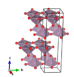
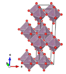
Figure 1: Crystal structure of $\alpha$-Mo in the $Pmcn$ space group setting. Viewed in terms of pyramidal or distorted octahedral units.

Table 2: Character table of $D_{2h}$.

irrep	$E$	$I$	$C_{2y}$	$m_{xz}$	$C_{2z}$	$m_{xy}$	$C_{2x}$	$m_{yz}$	basis function
$A_{g}$	1	1	1	1	1	1	1	1	$x^{2},y^{2},z^{2}$
$B_{1g}$	1	1	$-1$	$-1$	1	1	$-1$	$-1$	$xy$
$B_{2g}$	1	1	1	1	$-1$	$-1$	$-1$	$-1$	$xz$
$B_{3g}$	1	1	$-1$	$-1$	$-1$	$-1$	1	1	$yz$
$A_{u}$	1	$-1$	1	$-1$	1	$-1$	1	$-1$	$xyz$
$B_{1u}$	1	$-1$	$-1$	1	1	$-1$	$-1$	1	$z$
$B_{2u}$	1	$-1$	1	$-1$	$-1$	1	$-1$	1	$y$
$B_{3u}$	1	$-1$	$-1$	1	$-1$	1	1	$-1$	$x$

The character table of the point group $D_{2h}$ is given in Table 2. Further information on the space group operations is given in Appendix. Excluding the translations along the three directions, $x$, $y$ and $z$, the vibrational modes are distributed over the irreducible representations as

$$\Gamma^{vib}= 8A_{g}\oplus 4B_{1g}\oplus 4B_{2g}\oplus 8B_{3g}\oplus 4A_{u}$$ (1)

$$\oplus 7B_{1u}\oplus 7B_{2u}\oplus 3B_{3u}.$$

Of these modes, $A_{1u}$ modes are silent, the $B_{1u}$, $B_{2u}$ and $B_{3u}$ are infrared active and show a LO-TO splitting for electric fields along $z=c$, $y=b$, $x=a$. while $A_{g}$, $B_{1g}$, $B_{2g}$ and $B_{3g}$ are Raman active. More precisely, the Raman tensors are of the form

$$\left(\begin{array}[]{ccc}a&.&.\\ .&b&.\\ .&.&c\\ \end{array}\right), A_{g}$$ for , (5)

$$\left(\begin{array}[]{ccc}.&d&.\\ d&.&.\\ .&.&.\\ \end{array}\right), B_{1g}$$ for , (9)

$$\left(\begin{array}[]{ccc}.&.&e\\ .&.&.\\ e&.&.\\ \end{array}\right), B_{2g}$$ for , (13)

$$\left(\begin{array}[]{ccc}.&.&.\\ .&.&f\\ .&f&.\\ \end{array}\right), B_{3g}$$ for . (17)

For the monolayer structure, we consider only one “double layer” per cell and stack these directly on top of each other with large spacing in the $c$-direction. The space group then becomes $P2_{1}/m$, which is, in principle, monoclinic. In fact, a structure with this space group is described in Materials ProjectMP but with shorter interlayer distances. The layers then slide over each other and the structure becomes monoclinic with a $\alpha$-angle different from 90^∘. However, we space these layers much further to effectively study a single isolated monolayer and hence there is no driving force for this monoclinic distortion. The crystal structure in this case has $a=3.7217$ Å, $b=3.951$ Å, and $c=27.5832$ Å as optimized in LDA. In GGA-PBE, they are $a=3.7610$, $b=3.9693$, $c=28.8490$ Å. The point group in this case is $C_{2h}$ with the two-fold (screw) axis along $x$, a mirror-plane $m_{x}$ and the inversion center. The irreducible representation are given in the character table 3 and their relation to those in the $D_{2h}$ group is also given.

Table 3: Character table for $C_{2h}$ relevant to the monolayer MoO₃ and relation to parent irreducible representations of $D_{2h}$.

irrrep	$E$	$C_{2x}$	$m_{x}$	$i$	basis functions	$D_{2h}$ parent
$A_{g}$	1	1	1	1	$x^{2}$, $y^{2}$, $z^{2}$, $yz$	$A_{g}$, $B_{3g}$
$A_{u}$	1	1	$-1$	$-1$	$x$	$B_{3u}$
$B_{g}$	1	$-1$	$-1$	1	$xy$, $xz$	$B_{1g}$, $B_{2g}$
$B_{u}$	1	$-1$	1	$-1$	$y$, $z$	$B_{2u}$, $B_{1u}$

III.2 Phonon frequencies and related results.

The phonon frequencies at $\Gamma$ are given in Table 4 both in LDA (calculated with ABINIT) and in PBESOL (calculated with Quantum Espresso) and compared with experimental values. The PBEsol phonon calculation actually used the PBE optimized lattice constants from MPMP but with re-optimized internal coordinates. The reason for doing this, is that the $c$-lattice constant in PBEsol is clearly overestimated as mentioned earlier. Corresponding to the light polarized along z, x or y, the LO-TO splittings are observed for $B_{1u}$, $B_{3u}$ and $B_{2u}$ modes, respectively. From Table 4, we can observe that the splittings are significantly smaller for the lower frequency modes compared to the higher frequency modes. This is because only the high frequency modes have significant bond stretch dipolar character. The larger LO-TO splittings are also correlated with stronger oscillator strengths for infrared absorption.

Table 4: Phonon frequencies of $\alpha$-MoO₃ in cm^-1. Experimental values from Seguin et al Seguin et al. (1995).

$B_{1uT}$			$B_{1uL}$			$B_{2uT}$			$B_{2uL}$			$B_{3uT}$			$B_{3uL}$
LDA	PBEsol	expt	LDA	PBEsol	expt	LDA	PBEsol	expt	LDA	PBEsol	expt	LDA	PBEsol	expt	LDA	PBEsol	expt
$53.24$	21.44	53	$53.28$	21.45	53	$46.88$	34.21	44	$46.98$	34.22	44	$174.14$	178.87	191	$176.97$	179.29	191
$241.45$	247.52	260	$243.10$	248.78	260	$213.97$	231.24	228	$214.00$	231.67	228	$244.22$	234.86	268	$322.23$	336.30	343
$303.31$	339.02	353	$312.88$	342.76	363	$301.57$	339.47	348	$321.22$	344.22	352	$535.38$	477.63	545	$799.16$	785.11	851
$333.42$	348.93	374	$334.62$	349.09	380	$327.98$	348.49	363	$351.13$	357.70	390
$428.85$	429.52	441	$477.10$	476.65	505	$476.96$	477.74	500	$490.32$	491.40	525
$725.40$	766.50	814	$737.92$	773.37	825	$732.49$	774.77	818	$906.12$	942.66	974
$909.44$	983.48	962	$959.67$	1032.23	1010	$948.17$	1025.57	1002	$948.17$	1026.34	1002

$A_{g}$			$A_{u}$		$B_{1g}$			$B_{2g}$			$B_{3g}$
LDA	PBEsol	expt	LDA	PBEsol	LDA	PBEsol	expt	LDA	PBEsol	expt	LDA	PBEsol	expt
$73.44$	61.73	83	$48.84$	$27.85$	$101.50$	98.20	116	$117.27$	102.2	128	$89.94$	85.69	98
$151.43$	150.89	158	$211.03$	$202.02$	$183.80$	181.92	198	$224.88$	210.65	217	$146.16$	155.89	154
$195.69$	214.13	197	$263.01$	$244.13$	$258.69$	262.56	283	$270.29$	266.56	291	$227.42$	230.57	246
$299.00$	325.24	337	$535.78$	$478.26$	$651.88$	599.72	666	$652.04$	600.42	666	$302.60$	325.93	338
$329.83$	357.84	366									$342.49$	362.71	380
$445.84$	439.23	472									$447.71$	441.88	472
$727.19$	773.61	819									$729.82$	773.06	820
$945.50$	1022.51	996									$957.39$	1028.89	996

Our calculated values are compared with the experimental results of Seguin et al Seguin et al. (1995) who also includes previous experimental results and provides a symmetry labeling of the modes. However, we have relabeled them to take into account the different choice of crystallographic axes here. Our $a,b,c$ correspond to Seguin’s $c,a,b$. Taking $x,y,z$ along $a,b,c$ this then also implies that our $B_{1u},B_{2u},B_{3u}$ correspond to their $B_{2u},B_{3u},B_{1u}$ respectively and our $B_{1g},B_{2g},B_{3g}$ become their $B_{2g},B_{3g},B_{1g}$. $A_{g}$ and $A_{u}$ stay the same. The $A_{u}$ modes are silent and can thus not be measured by either infrared or Raman spectroscopies.

The calculated phonon frequencies are found to generally underestimate the experimental ones with a few exceptions. The largest absolute error in the LDA occurs for the $A_{g}^{7}$, $B_{3g}^{7}$ and the $B_{2u}^{6}$ modes, which are underestimated by about 80-100 cm^-1. The error on these modes is somewhat reduced in PBEsol but is still of order 50 cm^-1. On the other hand, the PBEsol seems to underestimate the low frequency modes significantly and its largest error now occurs for the $B_{3u}^{3}$, $B_{2g}^{4}$ and $B_{2g}^{4}$ modes. The root mean square error averaged over all TO modes and Raman modes is 39 cm^-1 in LDA and 29 cm^-1 in PBEsol, which is not a significant difference.

Some modes have quite weak oscillator strengths and, where several modes are close in frequency, the experimental assignment may not be entirely clear if polarization selection rules were not used. For example for mode $B_{1u}^{4}$, the value 374 cm^-1 was measured by Seguin et al Seguin et al. (1995) while Py and Mashke Py and Maschke (1981) give a calculated value $B_{1uT}^{4}=380$ cm^-1 but did not observe it experimentally. Seguin et al assign this mode as strong while nearby $B_{2u}$ mode at 358 cm^-1 (363 cm^-1 in Py and MashkePy and Maschke (1981) as listed in Table 4)is designated as weak. Another weak peak is observed in the IR spectrum at 350 cm^-1. The oscillator strengths given in Table 6 show clearly that $B_{1u}^{4}$ should be weaker than $B_{2u}^{3}$ and $B_{2u}^{4}$. The proximity of these modes makes it difficult to disentangle them experimentally without using polarization dependence.

One may also observe that each TO phonon mode of a given symmetry is followed by an LO before the next TO phonon occurs. This is a general rule obeyed by any crystal with at least orthorhombic symmetry, but not for monoclinic symmetry. We note that this follows from general considerations of the phonon related $\varepsilon$ and $\varepsilon^{-1}$ in a Lorentz oscillator model.

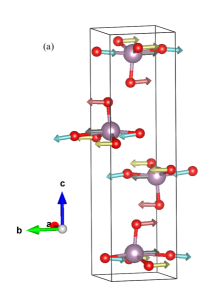
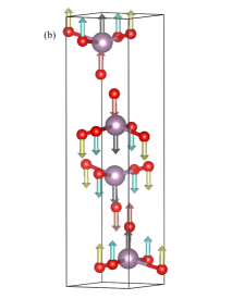
Figure 2: Eigendisplacement pattern for (a) $B_{1uT}^{1}$ mode and (b) $B_{2uT}^{1}$ modes.

We now discuss the nature of a few of the vibrational modes. The eigenvector displacements of all modes are given in Supplemental Information.SM The lowest frequency $B_{1u}^{1}$ corresponds to a sliding of an entire bilayer with respect to the other in the $b$ direction as can be seen in Fig. 2(a). The $B_{2u}^{1}$ mode on the other hand has bilayers moving relative to each other perpendicular to each other Fig. 2(b). One may expect these modes to be rather sensitive to the weak van der Waals like interlayer coupling. Because in PBEsol, the layers are somewhat farther apart, these mode frequencies are underestimated.

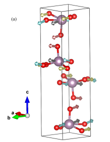
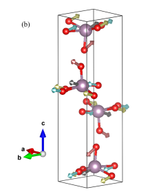
Figure 3: Eigendisplacement pattern for (a) $A_{g}^{1}$ mode and (b) $B_{3g}^{1}$ mode.

The $A_{g}^{1}$ mode on the other hand consists mostly of a sliding of the layers within one bilayer with respect to each other but also with a slight breathing component of the distance between these layers within the bilayer (Fig. 3)(a). This mode is already significantly higher in frequency which clearly shows that the bonding between layers within a bilayer is stronger than between bilayers. The lowest $B_{3g}^{1}$ mode is similar but with the two bilayers having opposite sign instead of the same sign (Fig. 3(b)). The $A_{g}^{2}$ and $B_{3g}^{2}$ modes are mostly a breathing mode of the interlayer distance within a bilayer but again, either in phase between the two bilayers or out of phase. The intermediate frequency modes are more complex in nature.

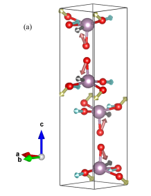
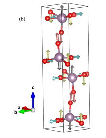
Figure 4: Eigendisplacement pattern for (a) $A_{g}^{7}$ mode and (b) $A_{g}^{8}$ mode.

However, the $A_{g}^{7}$ mode shows a strong Mo-O⁽¹⁾ bond stretch character with also some Mo-O⁽²⁾ stretch character, while $A_{g}^{8}$ is characterized by a stretch of the short Mo-O⁽²⁾ bond which explains why this mode has one of the highest frequencies. (See Figs. 4(a) and (b).)

It may be noticed that several modes are grouped in groups of four modes with frequencies close to each other. This is because the same local pattern can either be in phase or out of phase between the two Mo within a bilayer and between the two bilayers. Thus for example there are four modes close to 814 cm^-1 using the experimental value, they are the $A_{g}^{7}$, $B_{3g}^{7}$, $B_{1u}^{6}$, $B_{2u}^{6}$ modes. All of these are significantly underestimated and occur near 730 cm^-1 in LDA and near 770 cm^-1 in PBEsol. Because these modes involve strong motion along the $y=b$ direction, it has a strong coupling to an electric field along $y$ for the $B_{2uL}$ mode which occurs at 974 cm^-1. Similarly, there are four high frequency modes near 1000 cm^-1.

We find that the modes near 730 cm^-1, ($A_{g}^{7}$, $B_{3g}^{7}$, $B_{1u}^{6}$, $B_{2u}^{6}$) are quite sensitive to the interlayer distance. We can see this by comparing the PBEsol results at the PBEsol lattice constants with the PBEsol results at the PBE lattice constants which have respectively a $c$ lattice constant of 16.919 Å  and 14.425 Å. We find the phonon frequency decreases by $\sim$40 cm^-1 by using the larger interlayer distance. This suggests that further decreasing the lattice constant closer to experiment would reduce the error in this mode frequency. On the other hand, the highest modes increase only slightly in frequency (by about 4 cm^-1) when using the larger interplanar distance. This may also reduce the apparent overestimate of this mode by the PBEsol calculation.

III.3 Infared spectra and associated quantities.

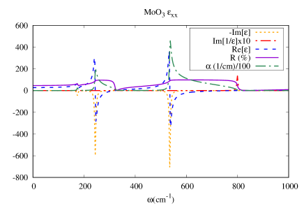
Figure 5: IR spectra for $B_{3u}$ modes.

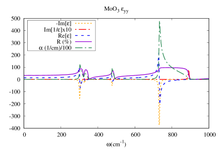
Figure 6: IR spectra for $B_{2u}$ modes.

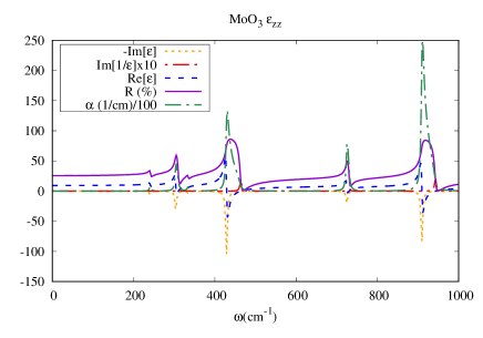
Figure 7: IR spectra for $B_{1u}$ modes.

Table 5: Born effective charge tensor elements for the atoms listed in Table 1. By symmetry all $Z^{*}_{xy}$, $Z^{*}_{yx}$, $Z^{*}_{xz}$, $Z^{*}_{zx}$ are zero.

Components(label)	Mo	O(1)	O(2)	O(3)
LDA
$Z^{*}_{xx}(A_{g})$	7.483	$-1.139$	$-0.552$	$-5.790$
$Z^{*}_{yy}(A_{g})$	6.649	$-4.859$	$-0.619$	$-1.169$
$Z^{*}_{zz}(A_{g})$	4.571	$-0.686$	$-2.275$	$-1.609$
$Z^{*}_{yz}(B_{3g})$	0.285	$-0.305$	$-0.343$	$-0.303$
$Z^{*}_{zy}(B_{3g})$	0.617	$-0.506$	$-0.350$	$-0.197$
PBEsol
$Z^{*}_{xx}(A_{g})$	7.632	$-1.115$	$-0.580$	$-5.940$
$Z^{*}_{yy}(A_{g})$	6.302	$-4.600$	$-0.601$	$-1.104$
$Z^{*}_{zz}(A_{g})$	4.268	$-0.563$	$-2.172$	$-1.532$
$Z^{*}_{yz}(B_{3g})$	0.290	$-0.304$	$-0.377$	$-0.354$
$Z^{*}_{zy}(B_{3g})$	0.553	$-0.438$	$-0.361$	$-0.223$

In this section, we present our simulated infrared spectra and associated quantities. All data reported here were obtained from the LDA calculation. These are obtained from calculating the contribution of phonons to the dielectric response function in terms of the classical Lorentz oscillator model. Within DFPT, the oscillator strengths can be obtained directly from the phonon eigenvectors and the Born effective charges, which describe the coupling of the vibrational modes to an electric field and are obtained as a mixed derivative of the total energy vs. a static electric field and an atomic displacement, given by

$$Z^{*}_{\kappa\beta\alpha}=\frac{\partial^{2}E_{tot}}{\partial u_{\kappa\alpha}\partial E_{\beta}}=V\frac{\partial P_{\beta}}{\partial u_{\kappa\alpha}}=\frac{\partial F_{\kappa\alpha}}{\partial E_{\beta}}$$ (19)

where $P_{\beta}$ is the macroscopic polarization, $V$ the unit cell volume and $u_{\kappa\alpha}$ the displacement of atom $\kappa$ in direction $\alpha$ which for a ${\bf q}=0$ mode is the same in each unit cell. $F_{\kappa\alpha}$ is the force on the atom $\kappa$ in direction $\alpha$ and $E_{\beta}$ is the electric field component. Atomic units are used throughout in which $\hbar=e=m_{e}=1$. Note that the Born effective charge tensors are not macroscopic tensors but only reflect the point group symmetry of the Wyckoff site of that atom. Because the atoms are all in $4c$ positions which lie on the mirror planes $m_{x}$ and hence need to have zero $xz$ and $xy$ tensor elements. However they do have a non-zero $yz$ and $zy$ element, which differ because the first index refers to the derivative vs. electric field and the second to the derivative vs. atom displacement direction. The Born charges are seen to deviate significantly from the nominal charge of Mo⁺⁶ and O^-2 and have also significant anisotropies. Specifically, O⁽²⁾ which is bonded to a single Mo in the $z$ direction is seen to be anomalously small in the $x$ and $y$ directions. On the other hand O⁽¹⁾ which is the bridge oxygen is seen to have the largest effective charge component in the $y$ direction and O⁽³⁾ in the $x$ direction. The off-diagonal $yz,zy$ elements sum to zero for each atom type separately because of the sign changes of the symmetry related atoms which behave as $B_{3g}$. The diagonal terms sum to zero for each diagonal component when summing over all atoms, balancing the cation and anions.

The oscillator strength is then given by

$$S_{n,\alpha\alpha}=\left|\sum_{\kappa,\alpha^{\prime}}Z^{*}_{\kappa,\alpha\alpha^{\prime}}U_{n}(\kappa,\alpha^{\prime})\right|^{2},$$ (20)

where $Z^{*}_{\kappa,\alpha\alpha^{\prime}}$ are the Born effective charge tensor components given in Table 5, $U_{n}(\kappa,\alpha^{\prime})$ are the eigenvectors for each of the modes $n$ at ${\bf q}=0$ and, $\kappa$ refers to the atom label. The eigenvectors are normalized as

$$\sum_{\kappa\alpha}U_{n}(\kappa,\alpha)^{*}M_{\kappa}U_{m}(\kappa,\alpha)=\delta_{nm},$$ (21)

where $M_{\kappa}$ are the atom masses. Note that because of the orthorhombic symmetry the oscillator strength tensor is diagonal. Its non-zero elements are listed in Table 6. One can see from this table, that the higher frequency modes tend to have higher oscillator strengths. This is because they correspond to bond stretches and thus have a significant dipole moment associated with them. An exception is the highest $B_{2u}^{7}$ mode has quite small oscillator strength and correspondingly also small TO-LO splitting.

Table 6: Oscillator strength tensors.

$S_{n,xx}$ $(B_{3u})$	$S_{n,yy}$ $(B_{2u})$	$S_{n,zz}$ $(B_{1u})$
$9.07\times 10^{-5}$	$3.05\times 10^{-7}$	$6.94\times 10^{-8}$
$1.67\times 10^{-3}$	$4.85\times 10^{-7}$	$1.559\times 10^{-5}$
$4.33\times 10^{-3}$	$5.94\times 10^{-4}$	$1.08\times 10^{-4}$
	$1.06\times 10^{-4}$	$1.07\times 10^{-5}$
	$2.73\times 10^{-4}$	$5.05\times 10^{-4}$
	$3.55\times 10^{-3}$	$1.62\times 10^{-4}$
	$2.22\times 10^{-9}$	$8.71\times 10^{-4}$

The frequency dependent dielectric function in the region below the band gap is given by

$$\varepsilon_{\alpha\alpha}(\omega)=\varepsilon_{\alpha\alpha}^{\infty}+\frac{4\pi}{V}\sum_{n}\frac{S_{n,\alpha\alpha}}{\omega_{n}^{2}-\omega^{2}-i\Gamma_{n}\omega}$$ (22)

where $\omega_{n}$ are the phonon frequencies and $\Gamma_{n}$ is a damping factor. The latter is not calculated and we just assign a uniform value of 5 cm^-1 to it for all modes.

The first term $\varepsilon^{\infty}$ is the high-frequency dielectric constant, meaning at frequencies below the gap but above the phonon frequencies. More precisely it is the static limit of the electronic contribution to the dielectric function, in other words the contribution from all higher frequency excitations, namely the inter-band optical transitions. It is calculated in the DFPT framework as the adiabatic response to a static electric field in the $x$, $y$, $z$ directions. Because of the orthorhombic symmetry it is also a diagonal tensor, $\varepsilon_{\alpha\alpha}^{\infty}$. The values of this tensor are given in Table 7. They are directly related to the anisotropic indices of refraction in the visible region below the gap but above the phonon frequencies. The values of $n_{\alpha\alpha}=\sqrt{\varepsilon_{\alpha\alpha}^{\infty}}$ are given in Table 8 for convenience. The static dielectric constant $\varepsilon^{0}_{\alpha\alpha}$ in Table 7 applies for frequencies well below the phonon frequencies.

Table 7: High-frequency and static dielectric tensor components.

method	$\varepsilon^{\infty}_{xx}$	$\varepsilon^{\infty}_{yy}$	$\varepsilon^{\infty}_{zz}$	$\varepsilon^{0}_{xx}$	$\varepsilon^{0}_{yy}$	$\varepsilon^{0}_{zz}$
LDA	6.792	6.162	4.662	27.210	13.024	7.173
PBEsol	5.959	5.205	4.001

Table 8: The indices of refraction.

method	$n_{xx}$	$n_{yy}$	$n_{zz}$
LDA	2.606	2.482	2.159
PBEsol	2.441	2.282	2.000

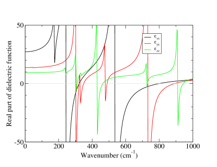
Figure 8: Real part of dielectric function for different directions.

From the above defined $\varepsilon(\omega)$ we can extract various related optical functions, in the infrared range. In particular, the optical absorption $\alpha(\omega)=2\omega\mathrm{Im}[\varepsilon(\omega)]/n(\omega)$ and the reflectivity $R(\omega)=|(\tilde{n}(\omega)-1)/(\tilde{n}(\omega)+1)|^{2}$ with $\tilde{n}=n+i\kappa=\sqrt{\varepsilon}$ the complex index of refraction as well as the loss function $-\mathrm{Im}\{\varepsilon(\omega)^{-1}\}$ are the most closely related to the measurements. The zeros in the real part $\varepsilon_{1}(\omega)=\mathrm{Re}[\varepsilon(\omega)]$ and the peaks in the loss function indicate the LO mode frequencies, while the peaks in $\varepsilon_{2}(\omega)=\mathrm{Im}\{\varepsilon(\omega\}$ give the TO modes. The reflectivity shows the typical Reststrahlen bands (RB) which jump to almost 100% reflectivity at the TO modes and fall back at the LO modes. Note that the absorption coefficient shows peaks corresponding to those in $\varepsilon_{2}(\omega)$ but also shoulders at the zeros of $\varepsilon_{1}(\omega)$. The infrared spectra for the three polarizations are shown in Figs. 5,6,7. These correspond respectively to $B_{1u}$, $B_{2u}$ and $B_{3u}$ modes which are active for polarizations along $z$, $y$ and $x$.

We may compare these with the IR absorption spectra of Seguin et al Seguin et al. (1995) which however do not mention the polarization. The highest absorption band found by them near 1000 cm^-1 agrees well with our $B_{1u}$ peak at 909-945 cm^-1 and corresponds to $z$-polarization, related to the Mo-O⁽²⁾ bond stretch of the shortest bond. The next main feature in Seguin et al Seguin et al. (1995) corresponds to our $B_{2u}$ spectrum for $y$-polarization and starts at $B_{2uT}^{6}$ at 732 cm^-1 and ends at the $B_{2uL}^{6}$ at 906 cm^-1. Note that this mode is also close to the strongest $A_{g}$ mode in Raman. However, the sharp feature on that peak at lower energy with much smaller LO-TO splitting is the $B_{1uT}^{6},B_{1uL}^{6}$ RB. The next broad feature is clearly dominated by the $B_{3u}^{3}$ RB between 535 cm^-1 and 799 cm^-1. In the lower frequency region, a RB occurs near 260 cm^-1 in the experiment, which corresponds to peaks in our spectra near 240 cm^-1 and stems mostly from the $x$ polarization $B_{3u}^{2}$ mode. A less intense RB is seen near 350 cm^-1 which corresponds to our $B_{2u}^{4}$ mode.

Table 9: Frequency ranges (cm^-1) with real $\varepsilon$ of different sign in different direcions, signs as indicated.

$\omega_{min}$	$\omega_{max}$	$\varepsilon_{xx}$	$\varepsilon_{yy}$	$\varepsilon_{zz}$
243	302	$-$	$+$	$+$
310	322	$-$	$-$	$+$
327	350	$+$	$-$	$+$
428	462	$+$	$+$	$-$
477	488	$+$	$-$	$+$
537	727	$-$	$+$	$+$
733	794	$-$	$-$	$+$
907	943	$+$	$+$	$-$

The anisotropy is important for this material. It leads to various ranges of wavenumber where $\varepsilon_{1}(\omega)$ has negative sign in one or two directions and positive in the other direction(s). This implies the material is hyperbolic in its dispersion in these ranges. Combined with low losses in these regions, or small imaginary part, this allows for interesting optical applications based on phonon-polaritons in the mid-infrared range.Ma et al. (2018); Dixit et al. (2021) Fig. 8 show the real part of the dielectric functions for the three directions together. One can see various ranges where the dielectric constant has opposite sign in different directions. These are summarized in Table 9. We should caution that we here have used an arbitrary broadening factor $\Gamma_{n}$ in the calculation of the dielectric function. Therefore we cannot at present accurately estimate the width of the peaks in the imaginary part $\varepsilon_{2}(\omega)$ which, in this context, is important in gauging the losses in propagating light.

III.4 Raman spectra

Table 10: Raman tensor components.

$A_{g}$	$A_{g}$	$A_{g}$
$a=\alpha_{xx}$	$b=\alpha_{yy}$	$c=\alpha_{zz}$
$1.99\times 10^{-3}$	$3.34\times 10^{-3}$	$-6.09\times 10^{-5}$
$-6.93\times 10^{-3}$	$-3.85\times 10^{-3}$	$-2.39\times 10^{-4}$
$3.84\times 10^{-3}$	$1.83\times 10^{-3}$	$-2.69\times 10^{-3}$
$1.04\times 10^{-2}$	$1.16\times 10^{-2}$	$-1.22\times 10^{-4}$
$-6.95\times 10^{-3}$	$3.32\times 10^{-3}$	$-3.98\times 10^{-4}$
$2.97\times 10^{-3}$	$4.26\times 10^{-3}$	$-9.03\times 10^{-3}$
$3.20\times 10^{-2}$	$7.01\times 10^{-2}$	$4.84\times 10^{-4}$
$1.52\times 10^{-2}$	$1.90\times 10^{-2}$	$3.04\times 10^{-2}$
$B_{1g}$	$B_{2g}$	$B_{3g}$
$d=\alpha_{xy}$	$e=\alpha_{xz}$	$f=\alpha_{yz}$
$3.24\times 10^{-3}$	$-3.09\times 10^{-3}$	$1.00\times 10^{-3}$
$-3.92\times 10^{-3}$	$3.67\times 10^{-3}$	$7.40\times 10^{-4}$
$1.17\times 10^{-2}$	$-9.62\times 10^{-3}$	$1.33\times 10^{-3}$
$9.17\times 10^{-3}$	$-1.72\times 10^{-2}$	$2.16\times 10^{-4}$
		$-7.88\times 10^{-3}$
		$1.26\times 10^{-3}$
		$8.75\times 10^{-4}$
		$-9.53\times 10^{-4}$

The Raman cross-section for the Stokes process (energy loss) for each mode is given by,

$$\frac{dS}{d\Omega}=\frac{(\omega_{0}-\omega_{m})^{4}}{c^{4}}|{\bf e}_{i}\cdot\bm{\alpha}^{m}\cdot{\bf e}_{o}|^{2}\frac{\hbar}{2\omega_{m}}(n_{m}+1)$$ (23)

where $\omega_{0}$ is the incident light frequency, $\omega_{m}$ the mode frequency, and $n_{m}$ is the phonon occupation number $n_{m}=[\exp{(\hbar\omega_{m}/k_{B}T)}-1]^{-1}$, ${\bf e}_{i}$ and ${\bf e}_{o}$ refer to the incident and the scattered polarization directions and $\bm{\alpha}^{m}$ is the second-rank Raman susceptibility tensor for mode $m$ which is given by,

$$\alpha^{m}_{\alpha\beta}=\sqrt{V}\sum_{\kappa\gamma}\frac{\partial\chi_{\alpha\beta}}{\partial\tau_{\kappa\gamma}}U_{m}(\kappa\gamma),$$ (24)

in terms of $U_{m}(\kappa\gamma)$,the eigenvector of the $m$-th vibrational mode and the derivative of the susceptibility vs. atomic displacements.

The results in this section were all obtained using the LDA calculations. The Raman tensor elements are given in Table 10. The Raman spectra for different scattering geometries, denoted by ${\bf k}_{i}({\bf e}_{i}{\bf e}_{o}){\bf k}_{o}$ with ${\bf k}_{i/o}$ the incident/scattered wavevector and ${\bf e}_{i/o}$ the incident and scattered light polarization are given in Figs. 9,10, 11 and 12. For $A_{g}$ modes corresponding to parallel polarizations, the intensity of the spectrum depends on the polarization selected. For $z(xy)z$ (transmission) or $z(xy)\bar{z}$ (reflection) one measures $B_{1g}$ modes, for $xz$-polarizations one measures $B_{2g}$ and for $yz$ polarization one measures $B_{3g}$ modes.

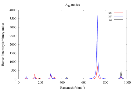
Figure 9: Raman spectra for $A_{g}$ modes.

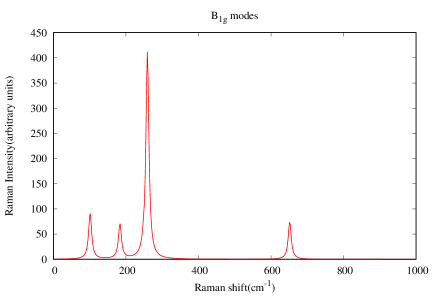
Figure 10: Raman spectrum for $B_{1g}$ modes, scattering geometry $z(xy)z$.

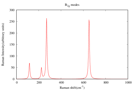
Figure 11: Raman spectrum for $B_{2g}$ modes, scattering geometry $y(xz)y$.

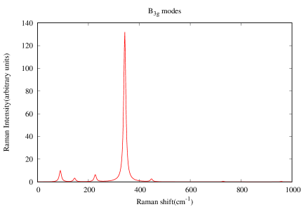
Figure 12: Raman spectrum for $B_{3g}$ modes, scattering geometry $x(yz)x$.

One can see that the $A_{g}$ have by far the strongest intensities. The $B_{3g}$ modes are the weakest. The strongest $A_{g}$ mode at 727 cm^-1 in $yy$ polarization corresponds to a mode with mostly in-plane eigendisplacements of Mo-O⁽¹⁾ bond stretches. It also has fairly strong $xx$ intensity but negligible $zz$ motion because it does not involve motions normal to the layer. On the other hand, the $A_{g}$ mode at 945 cm^-1 has its strongest polarization as $zz$ and corresponds to a Mo-O⁽²⁾ stretch mode. The strongest $B_{1g}$ mode is at 259 cm^-1 while the strongest $B_{2g}$ mode are at 270 cm^-1 and 652 cm^-1. All modes below $\sim 500$ cm^-1 are significantly weaker. The three most prominent modes, $A_{g}$ at 945 cm^-1, 727 cm^-1 and the $B_{1g}$ mode at 652 cm^-1 agree well with the experimental spectrum of Seguin et al Seguin et al. (1995) apart from our underestimates of these frequencies compared to the experiment.

III.5 Phonons in monolayer

Table 11: Phonon frequencies in cm^-1 for monolayer compared to bulk $\alpha$-MoO₃ in PBEsol. M indicates monolayer, B bulk. For bulk an average of $\{A_{g},B_{3g}\}$ is used for $A_{g}$, an average of $\{B_{1g},B_{2g}\}$ for $B_{g}$, $B_{3u}$ bulk corresponds to $A_{u}$ and an average of $\{B_{1u},B_{2u}\}$ for $B_{u}$.

$A_{g}$		$B_{g}$		$A_{uT}$		$A_{uL}$		$B_{uT}$		$B_{uL}$
M	B	M	B	M	B	M	B	M	B	M	B
$75.0$	$73.7$	$91.7$	$100.2$	$179.0$	$178.9$	$193.8$	$179.3$	$233.6$	$239.4$	$233.7$	$240.2$
$107.6$	$153.4$	$200.3$	$196.3$	$237.0$	$234.9$	$342.2$	$336.3$	$336.5$	$339.2$	$339.3$	$343.5$
$218.4$	$222.3$	$258.8$	$264.6$	$457.2$	$477.6$	$708.7$	$785.1$	$349.4$	$348.7$	$372.8$	$362.4$
$329.6$	$325.6$	$552.7$	$600.1$					$432.6$	$453.6$	$446.5$	$484.0$
$344.9$	$360.3$							$740.4$	$770.6$	$879.3$	$858.0$
$423.3$	$440.6$							$1006.5$	$1004.5$	$1006.8$	$1029.3$
$739.7$	$773.3$
$1011.7$	$1025.5$

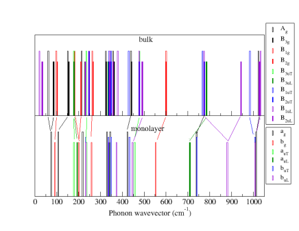
Figure 13: Comparison of bulk and monolayer phonon frequencies.

The phonons in a monolayer were calculated using the PBEsol exchange-correlation functional and using the PAW method. The results are shown in Table 11. They are compared with the corresponding average of modes in the bulk calculated with the same functional. As already mentioned in Table 3, there is a correspondence of irreducible representations of the monolayer point group to those of the bulk orthorhombic structure point group.

We note that we here treated the LO-TO splitting as in a 3D material. Strictly speaking, this is incorrect because in a monolayer, the LO-TO splitting goes to zero linearly in ${\bf q}_{\parallel}$ if we approach the $\Gamma$-point closely enough. One should thus interpret the LO mode frequency here as being for $|{\bf q}_{\parallel}|>1/r_{eff}$ with $r_{eff}$ an effective screening distance. This is due to the different nature of screening in a 2D material, which is unavoidably wave-vector dependent.Sohier et al. (2017) It is given by $\varepsilon_{2D}({\bf q}_{\parallel})=1+r_{eff}|{\bf q}_{\parallel}|)$, where ${\bf q}_{\parallel}$ is the wave vector parallel to the layer and $r_{eff}$ is an effective distance approximately given by $r_{eff}\approx\varepsilon_{\parallel}^{bulk}d_{M}/2$ with $d_{M}$ the thickness of the 2D monolayer.Sohier et al. (2017) Furthermore the Coulomb interaction in 2D has a different power dependence on $|{\bf q}_{\parallel}|$, namely $2\pi/|{\bf q}_{\parallel}$ instead of $4\pi/|{\bf q}|^{2}$ in 3D.

The correspondence with bulk mode and monolayer irreps was given in Table 3. The mode frequencies in bulk and monolayer are compared in Fig. 13. In the figure, we labeled monolayer irreps with lower case letters and color coded corresponding modes. The height of the bars in this bar graph has no physical meaning but helps to distinguish close lying modes. The lowest modes of the bulk do not occur in the monolayer because they correspond to motions in which entire double layers move with respect to each other. They are thus not included in Table 11 but are shown in Fig. 13. Several bulk (averages of corresponding modes) are seen to shift toward lower frequency in the monolayer, for example the ($A_{g}^{2}$, $A_{g}^{3}$, $A_{g}^{5}$, $A_{g}^{6}$, $A_{g}^{7}$, $A_{g}^{8}$) modes all have red-shifts. This is not too surprising since breaking even the weak bonds between layers would reduce the stiffness of the system and hence lead to smaller force constants and lower frequencies.

We can gain some more insights by looking specifically at the high frequency modes, which correspond to a clear bond stretch. For example the $A_{g}^{8}$, $B_{uT}^{6}$ modes both correspond to a Mo-O⁽²⁾ bond stretch in the $z$ direction. The bond stretch vibration can be estimated as

$$\omega\approx\sqrt{\frac{|K_{\mathrm{Mo}_{z},\mathrm{O}^{(2)}_{z}}|}{\mu}}$$ (25)

with

$$\frac{1}{\mu}=\frac{1}{m_{\mathrm{O}}}+\frac{1}{m_{Mo}}$$ (26)

the reduced mass if it were truly an isolated mode. Using a frequency of about 1000 cm^-1 this corresponds to a force constant of about 0.52 $e^{2}/a_{0}^{3}$ (or Hartree/Bohr²). Explicit calculations of the interatomic force constants show that this force constant is $-0.41$ $e^{2}/a_{0}^{3}$. However part of this force has long-range dipolar character and changes in screening may affect this dipolar part. Furthermore interactions across the van der Waals gap may also affect these O⁽²⁾-motion dominated modes. We here follow an analysis similar to that by Molina-Sánchez and WirtzMolina-Sánchez and Wirtz (2011) for MoS₂ and also used in Ref. Bhandari and Lambrecht, 2014 for V₂O₅.

First, we examine the changes in screening. The dielectric constant $\varepsilon^{\infty}$ of the monolayer is given in Table 12 and compared with the corresponding bulk as obtained within PBEsol. We can see that the dielectric constant in the plane is reduced by about a factor 2 and in the perpendicular direction by a factor 4. In fact, this dielectric constant is not really for a monolayer but for a periodic system of monolayers spaced by some large interlayer distance. For the $\varepsilon_{zz}^{\infty}$ we can think of it as a capacitor of thickness $d$ filled with a layer of thickness $d_{M}$ with dielectric constant $\varepsilon_{M}$ and vacuum in the rest. The effective dielectric constant of the capacitor is then given by $\varepsilon_{eff}^{-1}=1-\frac{d_{M}}{d}(1-\varepsilon_{M}^{-1})$. In our calculation, the monolayer has thickness $d_{M}\approx 6.6$ Å, while the $c$ lattice constant is about $d=28.3$ Å. This gives indeed an effective dielectric constant of 1.2, which is close to 1.44 in the actual calculation. Strictly speaking, the in-plane dielectric constant should become $\varepsilon_{\parallel}\approx 1+\varepsilon_{\parallel}^{bulk}d_{M}|{\bf q}_{\parallel}|/2$, meaning that for ${\bf q}_{\parallel}\approx 1/d_{M}$ it is $1+\varepsilon_{\parallel}^{bulk}/2$ but for ${\bf q}_{\parallel}\rightarrow 0$, so at large distance, it will approach 1.

Table 12: Dielectric constant of monolayer and bulk system.

	$\varepsilon_{xx}^{\infty}$	$\varepsilon_{yy}^{\infty}$	$\varepsilon_{zz}^{\infty}$
Monolayer	3.01	2.67	1.44
Bulk	5.95	5.20	4.00

Meanwhile it turns out that also the Born effective charges change significantly. For the monolayer calculation, they are given in Table 13 as obtained within PBEsol. We here give only the diagonal components. We can see that the $Z^{*}_{zz}$ is reduced by almost a factor 3 for the monolayer, while the in-plane components stay similar to the bulk.

Now, let’s consider the vibrational modes corresponding to the Mo-O⁽²⁾ bond stretch. The long-range dipolar force constant for this type of mode is

$$K^{LR}_{\mathrm{Mo}_{z},\mathrm{O}^{(2)}_{z}}=-2\frac{Z^{*}_{\mathrm{Mo}_{zz}}Z^{*}_{\mathrm{O}^{(2)}_{zz}}}{\sqrt{\varepsilon_{xx}\varepsilon_{yy}}d^{3}}$$ (27)

where $d$ is the Mo-O⁽²⁾ bond length. Clearly, because of the opposite sign Born charges, this interatomic force constant is positive. This is opposite to what a short-range spring would do. Indeed, if we move Mo in the $+z$ direction, the induced force on the O⁽²⁾ expected from a spring is also in the $+z$ direction to counteract the compression of the spring. But the definition $K_{i\alpha,j\beta}=-\partial F_{j\beta}/\partial u_{i\alpha}$ then implies a negative interatomic force constant. The strong Mo-O⁽²⁾ bond implies that the total force constant is negative and hence that the long-range part opposes the short range part. This is similar to the case of the V-O^vanadyl in V₂O₅.Bhandari and Lambrecht (2014). We can see that the Born charges here both are reduced by roughly a factor 3 while the denominator would be reduced by a factor 2 from bulk to monolayer. Hence the long range force constant is reduced by a factor $\alpha=0.22$. This dipolar part of the force constant from the above equation amounts to $\sim$0.10 $e^{2}/a_{0}^{3}$ (as confirmed by explicit calculation to be $+0.0993$ $e^{2}/a_{0}^{3}$) which is about 1/5 to 1/4 of the total force constant. The dipolar part being only a small part thus is essentially quenched in the 2D system and the force constant is reduced to only the short range part, which is larger. By itself this would then lead to an increase in net force constant in the monolayer and a blue shift by about 8%. However, the direct calculations shows a red-shift of smaller magnitude. This indicates that the above model of a localized isolated Mo-O⁽²⁾ bond vibration is not sufficient. We therefore surmise that the interaction between O⁽²⁾ in adjacent layers across the van der Waals gap must play a significant role and act as an attractive force in the bulk system outweighing the screening change effect. It turns out the O⁽²⁾ in one layer has interactions with four neighboring O${}^{(2)^{\prime}}$ in the adjacent double layer. These force constants are of order 0.0024$\pm 0.0002$ $e^{2}/a_{0}$ in $x,y,z$ direction. Evaluating their effect on the frequency would require a more detailed ball and spring model. They actually also have a substantial cancellation between long-range and short range components. It is clear however when these forces are removed by increasing the distance between the bilayers, then the frequency of the corresponding mode will be reduced. In V₂O₅ Bhandari and Lambrecht (2014) the corresponding O^vanadyl-O^vanadyl′ was negligible because of an almost exact compensation of the long-range and short range parts. We may note from the structure, that the O⁽²⁾ in adjacent layers in MoO₃ are much closer together laterally (their interatomic distance is about 2.89 Å) than the vanadyl oxygens in V₂O₅ (interatomic distance 3.72 Å). Thus, the situation here is more similar to that in MoS₂ for the out-of plane $A_{g}$ modes as considered in Ref. Molina-Sánchez and Wirtz, 2011. We may note that the two effects considered here oppose each other. The breaking of the weak interlayer interactions would lead to a red shift and the change in screening by itself would lead to a blue shift. Their compensation leads ultimately to only a small shift of these modes.

The modes $A_{g}^{7}$, $B_{uT}^{5}$ have a strong Mo-O⁽¹⁾ stretch character in the $y$ direction. This would involve a dipolar force constant of the form

$$K^{LR}_{\mathrm{Mo}_{y},\mathrm{O}^{(1)}_{y}}=-2\frac{Z^{*}_{\mathrm{Mo}_{yy}}Z^{*}_{\mathrm{O}^{(1)}_{yy}}}{\sqrt{\varepsilon_{xx}\varepsilon_{zz}}d^{3}}$$ (28)

In this case, one may notice that the Born charges barely change but the effective dielectric constant in the denominator is decreased by a factor 2.3. This would increase the dipolar part of the force constant in the monolayer compared to the bulk. The dipolar part in this case is again opposite to the short-range part and even larger, the total force constant $F_{yy}$ is found to be $-0.270$ while the short range part is $-0.574$ and the long-range part is $+0.304$ all in atomic units $e^{2}/a_{0}$. Thus, when the long-range part is increased by roughly a factor 2 the total force constant in this direction will be reduced in magnitude. This in turn can explain the red-shift encountered by this mode. This case differs from the MoS₂ case because there a Mo-Mo force constant is in play which has the opposite sign and hence leads to a blue shift for in-plane modes. It is similar to that case in the sense that the relevant Born charges do not change appreciably but the dielectric constant does. On the other hand these modes also have a bond stretch of the O⁽²⁾ involved in their motion, so our analysis of the corresponding mode shift is here somewhat oversimplified. These estimates are meant for the purpose of gaining insight only. We may expect from the analysis in the previous part that this part of the motion in the $z$ direction is again influenced by the O⁽²⁾-O^(2)′ interaction between atoms in adjacent double layers. Thus overall, a stronger red-shift is expected and this is confirmed by the direct calculations. It also agrees with the finding that this mode is particularly sensitive to the interlayer distance.

Table 13: Born effective charges in monolayer compared with bulk calculated in PBEsol.

atom	$Z^{*}_{xx}$	$Z^{*}_{yy}$	$Z^{*}_{zz}$
	monolayer
Mo	$7.822$	$6.427$	$1.562$
O(1)	$-1.181$	$-4.741$	$-0.208$
O(2)	$-0.513$	$-0.579$	$-0.819$
O(3)	$-6.135$	$-1.116$	$-0.543$
	bulk
Mo	$7.632$	$6.302$	$4.268$
O(1)	$-1.115$	$-4.600$	$-0.563$
O(2)	$-0.580$	$-0.601$	$-2.172$
O(3)	$-5.940$	$-1.104$	$-1.532$

IV Discussion and Conclusions

In this paper we have presented a DFPT study of the phonons in orthorhombic $\alpha$-MoO₃ with an emphasis on the Raman and infrared spectra. The calculated phonon frequencies both in LDA and in PBEsol were found to generally underestimate the experimental values slightly but give comparable errors. The nature of the phonon spectrum in terms of the eigenvectors was examined in some detail, explaining why the modes occur in groups of four.

The intensities in Raman spectra and the assignments of the major features are in good agreement with the experimental data reported in Seguin et al Seguin et al. (1995), which also include previously measured values.

Our paper also predicts shifts in some of the phonon frequencies in monolayer MoO₃ compared to bulk. The origin of these shifts was related to changes in the dielectric screening and Born effective charges between bulk and monolayer but also to the residual van der Waals interactions between the O⁽²⁾ sticking out from adjacent double layers.

While focusing on fundamental properties, our results may be anticipated to be useful in future characterization of MoO₃ for applications which require a thorough knowledge of the phonons. The polarization dependent Raman spectra given here and details given in Supplemental Material on each of the phonon patterns may be particularly useful to investigate changes in some phonon modes when hydrating the material or in some other way modifying the interlayer distances. An overview of applications of MoO₃ can be found in Ref. de Castro et al., 2017. Furthermore the well separated Restrahlen bands for different directions, with various ranges in the mid-infrared where the index of refraction is negative in one direction and positive in another provides opportunities for natural hyperbolic materials and low-loss phonon-polaritons.Ma et al. (2018); Dixit et al. (2021)

Supplementary Material: Figures of the eigendisplacements of all modes are provided.

Appendix A Space group symmetries

This appendix explains the space group symmetry operations in the $Pmcn$ setting we use. The left two columns of Table 14 correspond to the setting of the International Tables of Crystallography (ITC). The right two to the setting used in our paper. The first column gives a short cut notation for the symmetry operation, the second describes the symmetry operation including its location as follows: $2(00\frac{1}{2})(\frac{1}{4}0z)$ is the notation used in ITC, meaning a 2 fold screw axis $2_{1z}$ along the $z$-axis with $\frac{1}{2}$ translation along $z=c$ but located at $x=\frac{1}{4}$. The second column gives the operation in form $\{{\bf R}|\vec{t}\}$ where ${\bf R}$ is a rotation matrix and $\vec{t}$ is the non-primitive translation. Note that because the screw axis is located a $1/4$ along $a$ it requires not only a translation along the symmetry axis but also by 1/2 along $x$. In our notation this becomes a 2-fold screw axis along $y$ with extra translation along $z$ because it is located at $1/4$ along $c$. Applied to the coordinates of a Wyckoff $4c$ site with coordinates $(x,\frac{1}{4},z)$ this turns the atom in $(-x+\frac{1}{2},-\frac{1}{4},z+\frac{1}{2})$. In our notation the $4c$ Wyckoff position is $(\frac{1}{4},y,z)$ and this operation turns it into $(-\frac{1}{4},y+\frac{1}{2},-z+\frac{1}{2})$. where of course $-\frac{1}{4}$ can also be written $\frac{3}{4}$ because we can add any integer number to the fractional coordinates. Table 15 shows how the 4 atoms of the Wyckoff site $4c$ transform into each other and which symmetry operations relate them.

Table 14: Space group elements in two settings.

Pnma			Pmcn
$a>c>b$			$c>b>a$
$1$	$1$	$\left\{\left.\left(\begin{array}[]{ccc}1&&\\ &1&\\ &&1\end{array}\right)\right|(0,0,0)\right\}$	$1$	$1$	$\left\{\left.\left(\begin{array}[]{ccc}1&&\\ &1&\\ &&1\end{array}\right)\right|(0,0,0)\right\}$
$2_{1z}$	$2(00\frac{1}{2})(\frac{1}{4}0z)$	$\left\{\left.\left(\begin{array}[]{ccc}-1&&\\ &-1&\\ &&1\end{array}\right)\right|(\frac{1}{2},0,\frac{1}{2})\right\}$	$2_{1y}$	$2(0\frac{1}{2}0)(0y\frac{1}{4})$	$\left\{\left.\left(\begin{array}[]{ccc}-1&&\\ &1&\\ &&-1\end{array}\right)\right|(0,\frac{1}{2},\frac{1}{2})\right\}$
$2_{1y}$	$2(0\frac{1}{2}0)(0y0)$	$\left\{\left.\left(\begin{array}[]{ccc}-1&&\\ &1&\\ &&-1\end{array}\right)\right|(0,\frac{1}{2},0)\right\}$	$2_{1x}$	$2(\frac{1}{2}00)(x00)$	$\left\{\left.\left(\begin{array}[]{ccc}1&&\\ &-1&\\ &&-1\end{array}\right)\right|(\frac{1}{2},0,0)\right\}$
$2_{1z}$	$2(\frac{1}{2}00)(x\frac{1}{4}\frac{1}{4})$	$\left\{\left.\left(\begin{array}[]{ccc}1&&\\ &-1&\\ &&-1\end{array}\right)\right|(\frac{1}{2},\frac{1}{2},\frac{1}{2})\right\}$	$2_{1z}$	$2(00\frac{1}{2})(\frac{1}{4}\frac{1}{4}z)$	$\left\{\left.\left(\begin{array}[]{ccc}-1&&\\ &-1&\\ &&1\end{array}\right)\right|(\frac{1}{2},\frac{1}{2},\frac{1}{2})\right\}$
$-1$	$-1(000)$	$\left\{\left.\left(\begin{array}[]{ccc}-1&&\\ &-1&\\ &&-1\end{array}\right)\right|(0,0,0)\right\}$	$-1$	$-1(000)$	$\left\{\left.\left(\begin{array}[]{ccc}-1&&\\ &-1&\\ &&-1\end{array}\right)\right|(0,0,0)\right\}$
$m_{y}$	$m(x\frac{1}{4}z)$	$\left\{\left.\left(\begin{array}[]{ccc}1&&\\ &-1&\\ &&1\end{array}\right)\right|(0,\frac{1}{2},0)\right\}$	$m_{x}$	$m(\frac{1}{4}yz)$	$\left\{\left.\left(\begin{array}[]{ccc}-1&&\\ &1&\\ &&1\end{array}\right)\right|(\frac{1}{2},0,0)\right\}$
$a_{z}$	$a(xy\frac{1}{4})$	$\left\{\left.\left(\begin{array}[]{ccc}1&&\\ &1&\\ &&-1\end{array}\right)\right|(\frac{1}{2},0,\frac{1}{2})\right\}$	$c_{y}$	$c(x\frac{1}{4}z)$	$\left\{\left.\left(\begin{array}[]{ccc}1&&\\ &-1&\\ &&1\end{array}\right)\right|(0,\frac{1}{2},\frac{1}{2})\right\}$
$n_{x}$	$n(0\frac{1}{2}\frac{1}{2})(\frac{1}{4}yz)$	$\left\{\left.\left(\begin{array}[]{ccc}-1&&\\ &1&\\ &&1\end{array}\right)\right|(\frac{1}{2},\frac{1}{2},\frac{1}{2})\right\}$	$n_{z}$	$n(\frac{1}{2}\frac{1}{2}0)(xy\frac{1}{4})$	$\left\{\left.\left(\begin{array}[]{ccc}1&&\\ &1&\\ &&-1\end{array}\right)\right|(\frac{1}{2},\frac{1}{2},\frac{1}{2})\right\}$

Table 15: Transformation rule for Wyckoff position $4c$ in the space group $Pmcn$ setting. The last column lists the symmetry elements transforming the first atom to the one in that row.

$\frac{1}{4}$	$y$	$z$	$1$,$m_{x}$
$\frac{3}{4}$	$-y$	$-z$	$2_{1x}$,$-1$
$\frac{1}{4}$	$-y+\frac{1}{2}$	$z+\frac{1}{2}$	$2_{1z}$, $c_{y}$
$\frac{3}{4}$	$y+\frac{1}{2}$	$-z+\frac{1}{2}$	$2_{1y}$,$n_{z}$

References

- Rahmani et al. (2010) M. Rahmani, S. Keshmiri, J. Yu, A. Sadek, L. Al-Mashat, A. Moafi, K. Latham, Y. Li, W. Wlodarski, and K. Kalantar-zadeh, 145, 13 (2010).
- Balendhran et al. (2013a) S. Balendhran, S. Walia, M. Alsaif, E. P. Nguyen, J. Z. Ou, S. Zhuiykov, S. Sriram, M. Bhaskaran, and K. Kalantar-zadeh, ACS Nano 7, 9753 (2013a).
- Li et al. (2016) Y. Li, D. Wang, Q. An, B. Ren, Y. Rong, and Y. Yao, J. Mater. Chem. A 4, 5402 (2016).
- Voiry et al. (2013) D. Voiry, M. Salehi, R. Silva, T. Fujita, M. Chen, T. Asefa, V. B. Shenoy, G. Eda, and M. Chhowalla, Nano Letters 13, 6222 (2013).
- Kröger et al. (2009) M. Kröger, S. Hamwi, J. Meyer, T. Riedl, W. Kowalsky, and A. Kahn, Applied Physics Letters 95, 123301 (2009).
- Holler and Gao (2020) B. Holler and X. P. Gao, (2020), private communication.
- Balendhran et al. (2013b) S. Balendhran, J. Deng, J. Z. Ou, S. Walia, J. Scott, J. Tang, K. L. Wang, M. R. Field, S. Russo, S. Zhuiykov, M. S. Strano, N. Medhekar, S. Sriram, M. Bhaskaran, and K. Kalantar-zadeh, Advanced Materials 25, 109 (2013b).
- Sucharitakul et al. (2017) S. Sucharitakul, G. Ye, W. R. L. Lambrecht, C. Bhandari, A. Gross, R. He, H. Poelman, and X. P. A. Gao, ACS Applied Materials & Interfaces 9, 23949 (2017).
- Bhandari and Lambrecht (2014) C. Bhandari and W. R. L. Lambrecht, Phys. Rev. B 89, 045109 (2014).
- Mestl et al. (1994) G. Mestl, P. Ruiz, B. Delmon, and H. Knozinger, The Journal of Physical Chemistry 98, 11269 (1994).
- Py and Maschke (1981) M. Py and K. Maschke, Physica B+C 105, 370 (1981).
- Seguin et al. (1995) L. Seguin, M. Figlarz, R. Cavagnat, and J.-C. Lassègues, Spectrochimica Acta Part A: Molecular and Biomolecular Spectroscopy 51, 1323 (1995).
- Eda (1991) K. Eda, Journal of Solid State Chemistry 95, 64 (1991).
- Gonze (1997) X. Gonze, Phys. Rev. B 55, 10337 (1997).
- Gonze and Lee (1997) X. Gonze and C. Lee, Phys. Rev. B 55, 10355 (1997).
- Gonze et al. (2002) X. Gonze, J.-M. Beuken, R. Caracas, F. Detraux, M. Fuchs, G.-M. Rignanese, L. Sindic, M. Verstraete, G. Zerah, F. Jollet, M. Torrent, A. Roy, M. Mikami, P. Ghosez, J.-Y. Raty, and D. Allan, Computational Materials Science 25, 478 (2002).
- Gonze et al. (2020) X. Gonze, B. Amadon, G. Antonius, F. Arnardi, L. Baguet, J.-M. Beuken, J. Bieder, F. Bottin, J. Bouchet, E. Bousquet, N. Brouwer, F. Bruneval, G. Brunin, T. Cavignac, J.-B. Charraud, W. Chen, M. Côté, S. Cottenier, J. Denier, G. Geneste, P. Ghosez, M. Giantomassi, Y. Gillet, O. Gingras, D. R. Hamann, G. Hautier, X. He, N. Helbig, N. Holzwarth, Y. Jia, F. Jollet, W. Lafargue-Dit-Hauret, K. Lejaeghere, M. A. Marques, A. Martin, C. Martins, H. P. Miranda, F. Naccarato, K. Persson, G. Petretto, V. Planes, Y. Pouillon, S. Prokhorenko, F. Ricci, G.-M. Rignanese, A. H. Romero, M. M. Schmitt, M. Torrent, M. J. van Setten, B. Van Troeye, M. J. Verstraete, G. Zérah, and J. W. Zwanziger, Computer Physics Communications 248, 107042 (2020).
- Giannozzi et al. (2009) P. Giannozzi, S. Baroni, N. Bonini, M. Calandra, R. Car, C. Cavazzoni, D. Ceresoli, G. L. Chiarotti, M. Cococcioni, I. Dabo, A. D. Corso, S. de Gironcoli, S. Fabris, G. Fratesi, R. Gebauer, U. Gerstmann, C. Gougoussis, A. Kokalj, M. Lazzeri, L. Martin-Samos, N. Marzari, F. Mauri, R. Mazzarello, S. Paolini, A. Pasquarello, L. Paulatto, C. Sbraccia, S. Scandolo, G. Sclauzero, A. P. Seitsonen, A. Smogunov, P. Umari, and R. M. Wentzcovitch, Journal of Physics: Condensed Matter 21, 395502 (2009).
- Hartwigsen et al. (1998) C. Hartwigsen, S. Goedecker, and J. Hutter, Phys. Rev. B 58, 3641 (1998).
- Perdew et al. (1996) J. P. Perdew, K. Burke, and M. Ernzerhof, Phys. Rev. Lett. 77, 3865 (1996).
- He et al. (2014) L. He, F. Liu, G. Hautier, M. J. T. Oliveira, M. A. L. Marques, F. D. Vila, J. J. Rehr, G.-M. Rignanese, and A. Zhou, Phys. Rev. B 89, 064305 (2014).
- Veithen et al. (2005) M. Veithen, X. Gonze, and P. Ghosez, Phys. Rev. B 71, 125107 (2005).
- Blöchl (1994) P. E. Blöchl, Phys. Rev. B 50, 17953 (1994).
- Dal Corso (2014) A. Dal Corso, Computational Materials Science 95, 337 (2014).
- Perdew et al. (2008) J. P. Perdew, A. Ruzsinszky, G. I. Csonka, O. A. Vydrov, G. E. Scuseria, L. A. Constantin, X. Zhou, and K. Burke, Phys. Rev. Lett. 100, 136406 (2008).
- (26) Materials Project: https://materialsproject.org/, doi:10.1038/sdata.2018.65.
- (27) Supplemental Information contains figures of all vibrational mode eigendisplacements.
- Ma et al. (2018) W. Ma, P. Alonso-González, S. Li, A. Y. Nikitin, J. Yuan, J. Martín-Sánchez, J. Taboada-Gutiérrez, I. Amenabar, P. Li, S. Vélez, C. Tollan, Z. Dai, Y. Zhang, S. Sriram, K. Kalantar-Zadeh, S.-T. Lee, R. Hillenbrand, and Q. Bao, Nature 562, 557 (2018).
- Dixit et al. (2021) S. Dixit, N. R. Sahoo, A. Mall, and A. Kumar, Scientific Reports 11, 6612 (2021).
- Sohier et al. (2017) T. Sohier, M. Gibertini, M. Calandra, F. Mauri, and N. Marzari, Nano Letters 17, 3758 (2017), pMID: 28517939.
- Molina-Sánchez and Wirtz (2011) A. Molina-Sánchez and L. Wirtz, Phys. Rev. B 84, 155413 (2011).
- de Castro et al. (2017) I. A. de Castro, R. S. Datta, J. Z. Ou, A. Castellanos-Gomez, S. Sriram, T. Daeneke, and K. Kalantar-zadeh, Advanced Materials 29, 1701619 (2017).