Structural and dynamical properties of gel networks

Abstract

The competition of depletion attractions and longer-ranged repulsions between colloidal particles in colloid-polymer mixtures leads to the formation of heterogeneous gel-like structures. For instance, gel networks, i.e., states where the colloids arrange in thin strands that span the whole system occur at low packing fractions for attractions that are stronger than those at the binodal line of equilibrium liquid-fluid phase separation. By using Brownian dynamics simulations we explore the formation, structure, and ageing dynamics of gel networks. We determine reduced network that focus on the essential connections in a gel network. We compare the observed properties to those of bulky gels or cluster fluids. Our results demonstrate that both the structure as well as the (often slow) dynamics of the stable or meta-stable heterogenous states in colloid-polymer mixtures possess distinct features on various length and time scales and thus are richly divers.

I Introduction

In colloid-polymer mixtures the effective interaction between the colloids can be modelled by repulsions at very small and longer distances due to screend Coulomb interactions dlvo1 ; dlvo2 . At intermediate distances where there only is a small gap between the colloids that is too small for the polymers, depletion effects lead to an effective attraction between the colloids that is well described by the AO-approach ao ; vrij ; binder . The competition between the repulsive and the attractive interactions can lead to formation of complex ordered structures edelmann ; oguz . However, here we are interested in gels that occur in such a system verhaegh ; lu ; speck1 ; speck2 ; cho ; archer ; toledano ; zhang ; mani ; helgeson ; kohl ; doorn ; kohl2 .

In systems whith a strong attraction but no or only a small repulsion at a longer range clumpy gels are observed that occur when the system demixes into clusters at a high density and dilute pores in between verhaegh ; lu ; speck1 ; speck2 ; cho . In contrast, in case of the full competition between attraction and repulsion thin strands are observed that form network structures archer ; toledano ; zhang ; mani ; helgeson ; kohl ; doorn ; kohl2 . While in clumpy gels the slowdown of dynamics seems to occur due to an arrested fluid-liquid phase separation lu ; speck1 ; speck2 , in gel networks the slowdown usually is attributed to a percolation transition toledano ; mani ; helgeson ; kohl ; kohl2 . More specifically, the slowdown and the onset of ageing along with resulting phenomena like syneresis have been related to a directed percolation transition in space, i.e., the strands not only have to span the whole system but they have to do so in a directed way without any loops kohl ; kohl2 .

Note that in colloid-polymer mixtures both, clumpy gels as well as gel networks can be observed archer ; zhang ; mani ; helgeson . In equilibrium at sufficiently large packing fraction clumpy gels are observed in a similar way as for sticky particles without longer ranged repulsions, i.e., gelation in the sense of dynamically arrested states starts when the spinodal line of the fluid-liquid phase separation is crossed towards larger attractions, i.e., clumpy gels only occur for attractions larger than those at the binodal line zhang ; speck2 .

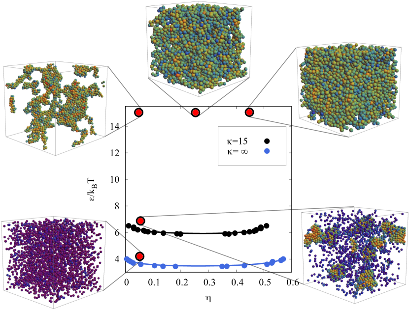
Figure 1: Phase diagram of the considered model system that resembles a colloid-polymer mixture. Details of the model are given in Sec II.1. The black line shows the binodal line of the gas-liquid phase separation for $\kappa$=15. For comparison, the blue line corresponds to the binodal line for purely attractive particles (i.e., for $\kappa=\infty$). The snapshots shown as insets illusutrate typical configurations at the given parameter sets (all for $\kappa$=15). Note that our system is similar to the one studied in speck2 and our binodal lines are in agreement with the one found in speck2 . However, no heterogeneous states have been reported in speck2 above the binodal line.

However, in dilute systems below a crossover packing fraction helgeson with sufficient longer-ranged repulsion the colloids organize in a filigree of thin strands toledano ; mani ; helgeson ; kohl ; kohl2 . In this article we refer to these structures when we use the term gel network. Obviously stable or at least meta-stable gel networks only occur for attractions that are stronger than at the equilibrium binodal line as otherwise the strands are not stable. As already mentioned, the dynamics of a gel network slows down and ageing sets in at the directed percolation transition toledano ; mani ; helgeson ; kohl ; kohl2 . In summary, for packing fractions above a crossover packing fraction the slowdown of dynamics is related to a liquid-fluid phase separation and results in clumpy gels. Percolation transitions are not important for these systems as they are usually all percolated speck2 . In contrast, for densities below the crossover packing fraction the slowdown leading to gel networks is related to a percolation transition that then usually occurs for attractions above the binodal line (see, e.g., helgeson for a complete picture).

We employ Brownian dynamics simulations to study the structure and dynamics in different states of a gel-forming colloid-polymer mixture. Note that the multiscale dynamics of a clumpy gel has previously been studied in cho but up to our knowledge we present an extensive analyzes of the dynamics on different lengths scales in gel networks for the first time.

As an overview of the different states considered in this article, we present an equilibrium phase diagram in Fig. 1 for orientation. We employ the model that previously has already been considered in speck2 . Details of the model are given in Sec. II. We are interested in the situation with competing short-range attractions and longer-ranged repulsions. The corresponding binodal line of demixing is indicated by a black line in Fig. 1, e.g., for smaller attractions the system always is fluid while for stronger attractions different stable or meta-stable cluster fluids and gel-like states are observed (see insets in Fig. 1). For example, close to the binodal line at small densities clusters are observed that can still move around as in a fluid as long as the system is not percolated. For stronger attraction percolated gel network structures occur at small packing fractions while for larger densities clumpy gels are observed. Our main interest in this work are the properties of the gel networks and how they differ from the cluster fluids or bulky gels.

Note that while we consider the model employed in speck2 our findings are in conflict to the claims in speck2 . In speck2 only systems with weak attraction, i.e., below or at the binodal line are considered. Nevertheless it was claimed that no other behavior could occur above the binodal line and especially that there was no transition between a cluster fluid and a gel network above the binodal line speck2 . Our observance of a cluster fluid above the binodal already already proves that in speck2 the findings from below the binodal lines have wrongly been generalized to systems above the binodal line. Our main focus lies on structures with stronger attractions, i.e., above the binodal line.

The article is organized as follows: In Sec. II we first introduce the model system, before we describe the Brownian dynamics simulations, and our methods of analyzes. In Sec. III we present our simulation results concerning the thermalization process, the structure, as well as the dynamical properties of gel networks. Finally, we conclude in Sec. IV.

II Model and simulation details

II.1 Model details

We perform Brownian dynamics simulations in a system closely related to the one presented in speck2 consisting of $N$ collidal particles whose radii are drawn from a Gaussian distribution, such that the polydispersity of the system is 5%. The mean diameter of the particles is called $\sigma$ and the sum of radii of particles $i$ and $j$ is $\sigma_{ij}$. The short range attraction is modeled via a modified square-well potential $U_{\text{SW},ij}(r)$ of width $\delta=0.03\sigma$ and depth $\epsilon$, the longer ranged repulsion is given by a Yukawa potential $U_{\text{YK},ij}(r)$ which models screened electrostatic repulsion. The overall interaction potential shown in Fig. 2 is the sum $U_{\text{tot},ij}(r)=U_{\text{YK},ij}(r)+U_{\text{SW},ij}(r)$ where $\displaystyle U_{\text{YK},ij}(r)$ $\displaystyle=C\left(\frac{2}{2+\kappa\sigma_{ij}}\right)^{2}\left(\frac{\sigma_{ij}}{r}\right)\text{exp}[-\kappa(r-\sigma_{ij})],$ $\displaystyle U_{\text{SW},ij}(r)$ $\displaystyle=\begin{cases}-\frac{\epsilon}{2\alpha}r+\frac{\epsilon(1-\alpha)}{2\alpha}&\text{if }r<\sigma_{ij}+\alpha\\ -\epsilon&\text{if }\sigma_{ij}+\alpha\leq r\leq\sigma_{ij}+\delta-\alpha\\ \frac{\epsilon}{2\alpha}r-\frac{\epsilon(1+\delta+\alpha)}{2\alpha}&\text{if }\sigma_{ij}+\delta-\alpha<r<\sigma_{ij}+\delta+\alpha\\ 0&\text{else}.\end{cases}$ The additional parameter $\alpha$ flattens the wells of the square-well potential, which is necessary to avoid inifite forces when performing Brownian dynamics simulations. In our simulations we choose $\alpha=\frac{\delta}{5}$. The screening length $\kappa^{-1}$, which represents the strength of the repulsive force, can be tuned by modifying salt concentration in experiments kohl . $\kappa=\infty$ represents the case of a purely attractive potential without repulsive forces. The parameter $C$ is chosen as 200$k_{B}T$. The cut-off distance is chosen to be $\frac{r_{\text{Cut}}}{\sigma}=1+\frac{4}{\kappa}$ as in speck2 . In summary the whole system can be characterized by choosing a triplet of parameters $(\epsilon,\kappa,\eta)$, where $\eta=\frac{\pi}{6}\sigma^{3}\frac{N}{L^{3}}$ is the packing fraction of the system with the box size $L$. Note that in the following $\epsilon$ is used in units of $k_{B}T$ and $\kappa$ in units of $\sigma^{-1}$.

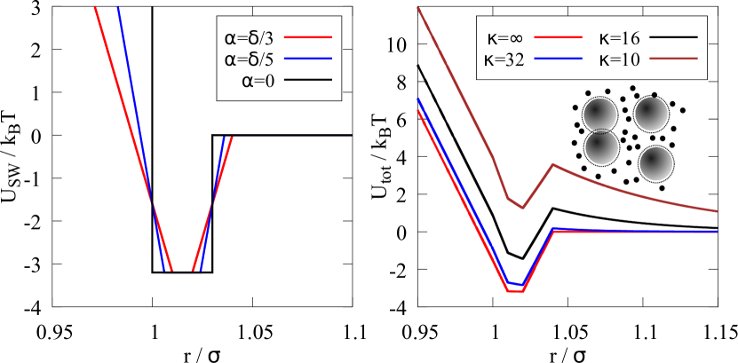
Figure 2: The overall potential (shown in the right panel for different screening lengths $\kappa^{-1}$) is a sum of a repulsive Yukawa potential $U_{YK}$ and a modified square-Well-Potential $U_{SW}$ (depicted on the left hand side) with width $\delta=0.03\sigma$. To avoid infinite forces the jumps in the square well potential are smoothened by introducing a parameter $\alpha$ as given in the text. In the rest of the article $\alpha=\frac{\delta}{5}$ is used. In the examples shown here, the strength of the attraction always is $\epsilon=3$.

II.2 Brownian Dynamics

We employ Brownian dynamics simulations where the motion of colloidal particles in a solvent is determined by numerically integrating the overdamped Langevin-equation for particle $j$

$$\gamma\frac{d}{dt}\vec{r}_{j}=\vec{F}_{\text{int}}+\vec{F}_{\text{th}},$$

where $\gamma$ is the friction constant, $\vec{F}_{\text{int}}$ models the effective force between colloidal particles as given by the pair interaction potential introduced in the pevious subsection, and $\vec{F}_{\text{th}}$ denotes random forces due to thermal fluctations. It is $\left\langle\vec{F}_{\text{th}}\right\rangle=\vec{0}$ and $\left\langle F_{\text{th},i}(t)F_{\text{th},j}(t^{\prime})\right\rangle=2\gamma k_{\textnormal{B}}T\delta_{ij}\delta(t-t^{\prime})$. The time steps in our simulations are $\Delta t=10^{-5}\tau_{B}$ with the Brownian time $\tau_{B}=\frac{\sigma^{2}\gamma}{4k_{\textnormal{B}}T}$. The calculation of forces was done using a combination of the Verlet-list algorithm and the linked-cell algorithm to reduce computation timeallen . For $\eta=0.05$ boxes of size $30\sigma\times 30\sigma\times 30\sigma$ with periodic boundary conditions are used and filled with colloids until the considered packing fraction is reached, i.e., we simulate with $N=2578$ particles. For $\eta=0.25$ we use boxes of size $20\sigma\times 20\sigma\times 20\sigma$ and $N=3819$ particles.

II.3 Reduced Networks

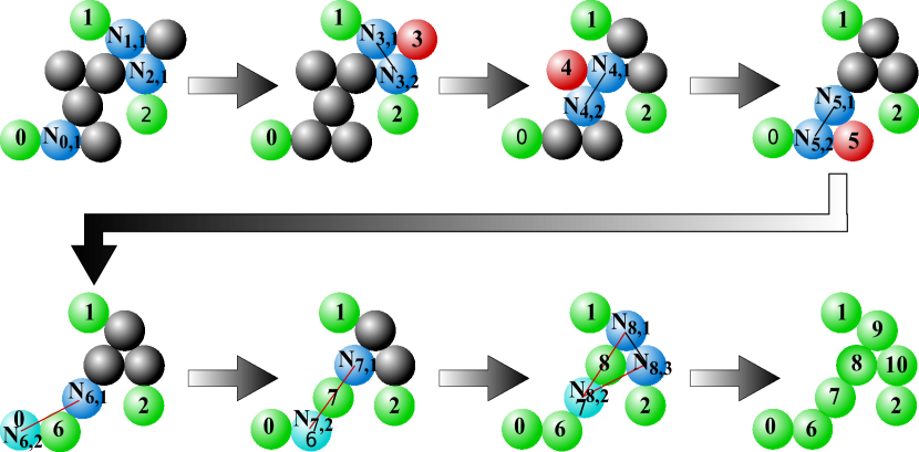
Figure 3: Schematical representation of the algorithm developped to determine a reduced network. Starting with the particle $i$ which has the minimal coordination number. If the neighbors $N_{i,j}$ are still connected when the chosen particle $i$ is removed it will be removed, otherwise it is kept and marked as visited. Removed particles are shown in red, visited and kept particles in green. The algorithm continues until every particle has been visited.

Complex network structures occur in some regions of the phase diagram (see e.g. Fig. 1). To extract the essential part of these networks, we determine so-called reduced networks. The key idea is to remove as many particles as possible without destroying connections within the network. The algorithm is illustrated in Fig. 3 and works as follows

• Remove all single particles which have no neighbors.

• Choose the particle $i$ with the minimal number of neighbors.

• Check whether particle $i$ was already chosen before.

  • Keep particle $i$ and start again at step 1 (ignoring particle $i$ from now on).

  • Calculate all neighboring particles $N_{i,j}$ for the chosen particle $i$ and check whether these are still connected over a certain amount of steps (we choose 3 steps) if $i$ would be removed.

    • Delete particle $i$.

    • Keep particle $i$ and mark it as visited.

• Start again at step 1, until every particle has been marked as visited.

• When every particle was visited start the algorithm again with the reduced network as initial configuration until no more particles are removed during the whole procedure.

The results of this analysis is shown later within this work, e.g., Fig. 7.

III Results

III.1 Initial evolution towards heterogeneous structure

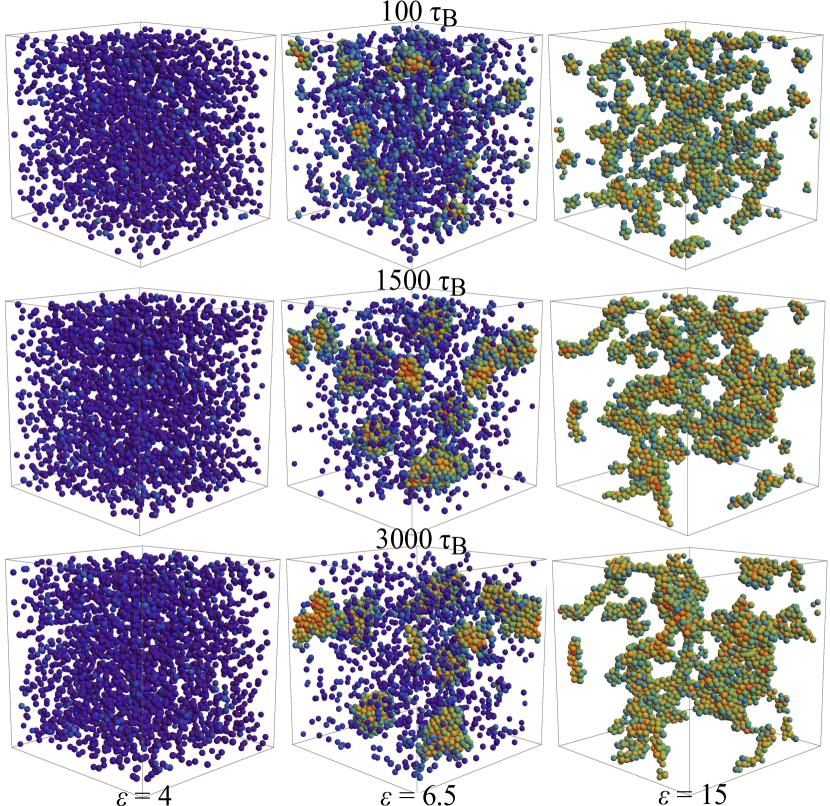
Figure 4: Evolution of the system for an inverse screening length $\kappa=15$ at a packing fraction $\eta=0.05$ for attraction strength $\epsilon=4$ (left column), $\epsilon=6.5$ (center column), and $\epsilon=15$ (right column). The colors indicate the number of nearest neighbors each particle has, ranging from blue for no neighbors to red for 12 neighbors.

We first study how the particles that are initially placed at random positions organize to form the heterogeneous structures that we are interested in. In Fig. 4 we show snapshots of the evolution for different systems at a low packing fraction of $\eta=0.05$ and different strength of attraction $\epsilon$ after $100\tau_{B}$, $1500\tau_{B}$, and $3000\tau_{B}$ where $\tau_{B}$ is the Brownian time introduced in Sec. II.2. The case shown in the left column of Fig. 4 with an attraction strength $\epsilon=4$ is on the fluid side of the binodal line. Therefore, no complex structures occur. On the opposite side of the binodal line, i.e., where phase separation is expected in equilibrium, heterogeneous structures are observed. Depending on the attraction strength different regimes can be observed. To be specific, close to the binodal line, e.g., for $\epsilon=6.5$, unconnected clusters of particles are found (center column). As these clusters can move freely, we term this state a cluster fluid. Far above the binodal line, e.g., for $\epsilon=15$ as shown in the right column, a gel network with percolating strands is formed. Furthermore, unbound particles are rare in such gel networks.

The initial structure formation occurs within a short time. Already after $100\tau_{B}$ (top row of Fig. 4) the most important features of a structure are visible. Not that between $100\tau_{B}$ and $1500\tau_{B}$ (center row) there are still structural changes visible in case of the heterogeneous structures. However, between $1500\tau_{B}$ and $3000\tau_{B}$ no significant changes of the type of structure is visible from the snapshots, i.e., the system seems to relax towards a meta-stable structure. We now want to study this initial relaxation process in more detail and characterize the evolution of the structures quantitatively.

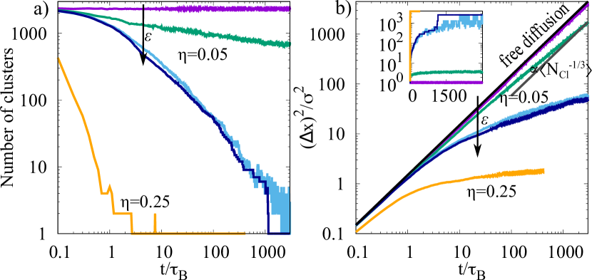
Figure 5: (a) Number of non-connected clusters and (b) mean squared displacement $(\Delta x)^{2}/\sigma^{2}$ in the system during the inital relaxation. The inset in (b) shows the mean cluster size. The light-orange curve is a clumpy gel for $\eta=0.25$ and $\epsilon=15$ while all other curves denote systems at a low packing fraction $\eta=0.05$ and various attraction strengths ranging from a fluid with $\epsilon=4$ (purple), over a cluster fluid with $\epsilon=6.5$ (green), to percolating gel networks with $\epsilon=9$ and $\epsilon=15$ (light-blue and dark-blue, respectively). Note that the colors are the same as specified in the legend of Fig. 6 and are used throughout the rest of the article for all low density systems. The black line in (b) denotes free diffusion with $(\Delta x)^{2}/\sigma^{2}=3t/(2\tau_{B})$ and the grey curve indicates $(\Delta x)^{2}/\sigma^{2}=3t/(2\tau_{B})\left\langle N_{\textnormal{Cl}}^{-1/3}\right\rangle$, where $\left\langle\cdot\right\rangle$ indicates the average over all particles and $N_{\textnormal{Cl}}$ is the size of the cluster around a particle at $3000\tau_{B}$ for the cluster fluid ($\epsilon=6.5$).

Fig. 5a) shows the number of clusters forming in a system and in the inset of Fig. 5b) the mean cluster size is plotted. For low packing fraction $\eta=0.05$ the evolution strongly depends on the attraction strength. Below the binodal line, i.e., in the fluid phase shown by purple lines, particles hardly attach to each other such that the number of clusters remains large and the mean cluster size small. For the cluster fluid in the phase separated part of the phase diagram close to the binodal line, represented with green curves, the growth of clusters can be observed that significantly slows down for larger times though some slow evolution is still ongoing at the end of this initial simulation. The gel networks depicted with light-blue and dark-blue curves slowly relax towards percolated states, i.e, finally all particles are part of one connected (network) structure. For comparison, the case of a clumpy gel with a packing fraction of $\eta=0.25$ and a strong attraction of $\epsilon=15$ (light-orange curves) is shown. It percolates much faster, namely within a few Brownian times.

In Fig. 5(b) the mean-squared displacement during the initial relaxation process is shown. In a fluid phase diffusive behavior is expected in the long time limit. Indeed, for the fluid state below the binodal line, the particles move as expected from free diffusion which we indicate by a black line that lies on top of the purple curve. In case of a cluster fluid the mean-squared displacement can be roughly estimated by considering diffusion of clusters whose size corresponds to the mean cluster size that we observe at $3000\tau_{B}$. If the clusters had a spherical shape one would expect that the diffusion constant is lowered by a factor $\left\langle N_{\textnormal{Cl}}^{-1/3}\right\rangle$ (see grey line in Fig. 5(b)). We indeed find that the mean-squared displacement of the cluster fluid approaches this estimated diffusive behavior.

In contrast, the mean-squared displacement of the particles in gel networks (light-blue and dark-blue curves) flattens significantly. As a consequence, it is still possible that the mean-squared displacement of gel networks will reach a diffusive limit at a much longer time. However, on the timescale accessible for our simulations, the system behaves subdiffusively. Therefore, the dynamics slows down significantly but is not completely arrested. The remaining dynamics can be considered as ageing process.

III.2 Structure

As seen in the previous section the evolution of gel networks slows down dramatically after an initial thermalization period. Note that the system is not in perfect equilibrium and not static after the thermalization. However, changes of the structure become very slow and will be considered as ageing dynamics of an effectively meta-stable state. In this subsection, we want to study the structure of the heterogeneous states after the initial relaxation dynamics.

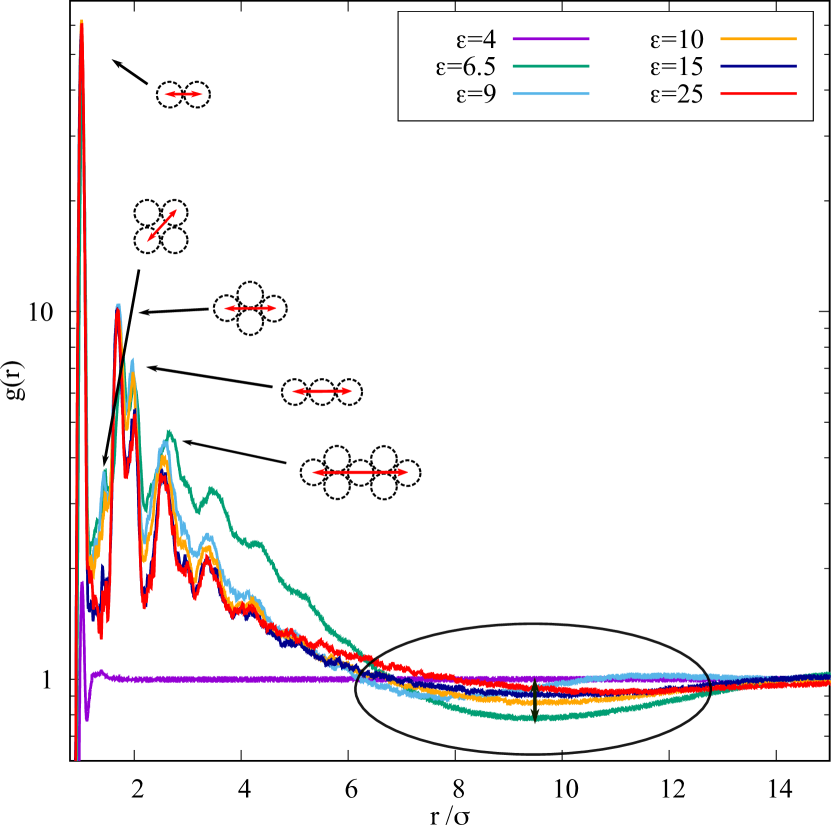
Figure 6: Radial pair correlation functions $g(r)$ for $\kappa=15$, $\eta=0.05$, and different attraction $\epsilon$. The purple curve $\epsilon=4$ is taken below the binodal and shows typical like behavior of a homogeneous fluid, while all other pair correlation functions taken above the binodal show signitures of cluster or network structures. Preferred particle configuration can be identified by studying peak positions. The mean distance of the region where $g(r)<1$ can be seen as a measure of the mesh size of a network in case of the gel networks or as typical distance to void spaces between clusters in case of the cluster fluid.

Fig. 6 shows the pair correlation function $g(r)$ for low packing fractions $\eta=0.05$, a screening length given by $\kappa=15$, and different values of $\epsilon$. Note that the data was averaged over 500$\tau_{B}$ after an initial thermalization time of 2500$\tau_{B}$. In the homogeneous fluid below the binodal line, i.e., for $\epsilon=4$ (purple curve) peaks are less pronounced then in the inhomogeneous structures above the binodal line, where the peaks can be assigned to preferred particle configurations. Close to the binodal line ($\epsilon=6.5$, green curve) an extended cluster can be observed up to distances of approximately $6\sigma$ followed by a void region with $g(r)<1$. For the gel networks with larger $\epsilon$ the initial region with $g(r)>1$ decays faster but does hardly differ for different $\epsilon$. The mean distance of the region with $g(r)<1$ can be associated to the mesh size of the networks. As can be seen in Fig. 6 the mesh size increases with increasing $\epsilon$.

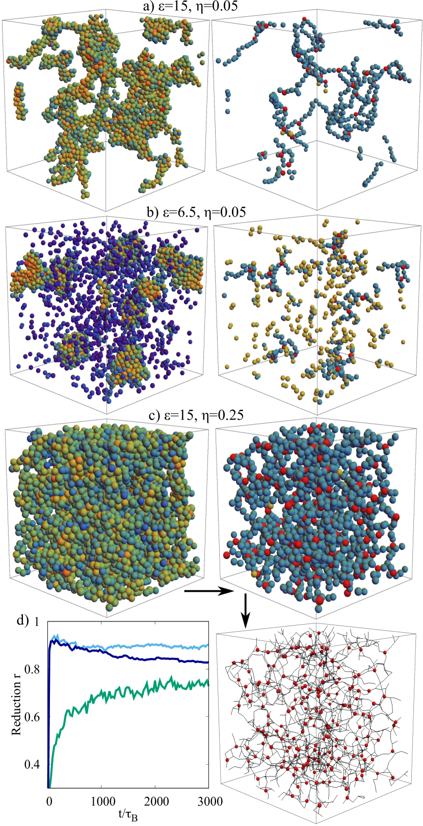
Figure 7: (a,b,c) Snapshots of typical heterogeneous structures (left panels) where particles are colored by their number of neighbors as in Fig. 4 and the corresponding reduced networks constructed by the method introduced in Sec. II.3 (right panels) where red particles represent nodes, blue particles are colloids in strands, and yellow particles denote the end of strings. (a) Gel networks for $\epsilon=15$, $\kappa=15$, and $\eta=0.05$ after 3000$\tau_{B}$. (b) Cluster fluid for $\epsilon=6.5$, $\kappa=15$, and $\eta=0.05$ after 3000$\tau_{B}$. (c) Clumpy gel for $\epsilon=15$ , $\kappa=15$, and $\eta=0.25$ after 400$\tau_{B}$ for comparison. In the bottom panal on the right hand side we have redrawn the reduced network structure of the clumpy gel with only showing node particles in red and lines for connections between particles in the reduced network. (d) Fraction of particles that are left away while constructing a reduced network after different relaxation times. Note that unbounded particles had already been omitted before the reduced network was constructed. The same colors as in Fig. 6 are used, i.e., the blue curves are the results of gel networks and the green curve for the cluster fluid.

Next we determine typical reduced network structures as introduced in Sec. II.3. In Fig. 7 three examples are shown, namely a gel networks in (a), a cluster fluid in (b), and a clumpy gel in (c). While the cluster fluid is obviously unpercolated, the shown gel network just percolates. Note that one has to take the periodic boundary conditions into account to see the percolation. For both, the cluster fluid as well as the gel networks, the reduced networks only consists of a small fraction of the original particles. In contrast, the reduced network of a clumpy gel that we analyze in comparison in Fig. 7(c) possesses a dense structure, i.e., no significant void regions are visible.

For gel networks and the cluster fluid we show in Fig. 7(d) the fraction of particles which can be removed during the construction of a reduced network after initially all single particles have already been removed. In gel networks for $\epsilon=9$ (light-blue) and $\epsilon=15$ (dark-blue) most particles can be removed, i.e., most colloids are not essential for the connections in a network. Initially, both gel networks behave similarly, but after about 1000$\tau_{B}$ the fraction of removed particles for $\epsilon=9$ remains constant, while for $\epsilon=15$ it decreases. A possible interpretation of this behavior is that for $\epsilon=15$ thinner strands form which do not allow a high removal rate, because otherwise connections would be destroyed.

In contrast, for cluster fluid with $\epsilon=6.5$ (green curve) fewer particles can be removed, especially in case of smaller relaxation times. The reason is that the cluster fluid consists of unconnected clusters and in each of these clusters some particles have to remain in order to denote the connections within the cluster. The increase of the green curve in Fig. 7(d) results from the decrease of the number of clusters during the initial thermalization.

III.3 Dynamics of network structure

In this subsection, we explore the dynamics of the heterogeneous structures after an initial relaxation process. This dynamics can be considered as ageing dynamics or as a (slow) continuation of the relaxation.

III.3.1 Spatial correlations

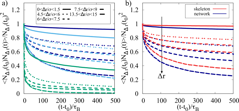
Figure 8: Correlation functions $\left\langle N_{\Delta r}(t_{0})N_{\Delta r}(t)\right\rangle$ indicating what fraction of particles that initially are at a spatial distance $\Delta r$ from within the intervals given in the legend stay within these intervals up to the time $t$. A detailed definition of $N_{\Delta r}(t)$ is given in the text. Data is averaged over at least 4 individual runs to increase the statistics and the initial relaxation time is $t_{0}=3000\tau_{B}$. (a) Correlation functions for gel networks (dark-blue for $\epsilon=15$ and light-blue for $\epsilon=9$) and a cluster fluid (green, $\epsilon=6.5$). In all cases, $\kappa=15$ and $\eta=0.05$. The line style denotes the intervals of the spatial distance as specified in the legend. (b) Correlation functions for the case $\epsilon=15$, function evaluated for all particles in comparison to the correlations only determined for the particles that are part of the reduced network (skeleton). The correlation of particles in the reduced network is stronger which can be explained by boundary particles at the outside of strings which are removed in the skeleton. These are able to leave the string and can move easier.

For the particles that at a time $t_{0}$ have been at a spatial distance $\Delta r$ from an arbitrarily chosen reference particle, we first determine the number of particle $N_{\Delta r}(t)$ that at time $t$ have not left a certain interval around the distance $\Delta r$. Note that particles that during some time are closer or further away than allowed by the chosen interval are no longer counted even if they return at a later time. In the next step we calculate the correlation function $\left\langle N_{\Delta r}(t_{0})N_{\Delta r}(t)\right\rangle$ which by construction is a monotonously decreasing function.

In Fig. 8(a) the correlation functions are shown for two gel-networks (light-blue and dark-blue) as well as for the cluster fluid (green). For the cluster fluid the correlation functions decay much faster than for the gel networks. Only for small $\Delta r$ a significant amount of particles stay at a similar distance which probably are particles within the same cluster. For larger distances the rapid decay for the cluster fluid indicates that the clusters in a cluster fluid are unconnected and therefore can move around freely.

For the gel networks the decay is more pronounced for larger distances indicating that some network rearrangements still are possible. The most pronounced differences between the two gel networks occur for the case of small distances: For particles that were neighbors in the beginning, the correlations for $\epsilon=9$ decay faster than for $\epsilon=15$ because bonds between particles can rupture much easier in case of smaller attractions. Interestingly, while some small differences are visible for the different gel networks in most cases, for a distance in the range $6\sigma$ to $7\sigma$ hardly any difference between the correlation functions can be noticed. Note that this distance approximately corresponds to half a mesh size as expected from Fig. 6. For shorter distances particles that disconnect or connect to strands probably make a difference, while the difference for larger distances is due to network rearrangements that occur on the length scale of the mesh size or even larger length scales.

It is also possible to calculate the spatial correlation functions for the particles which are part of the corresponding reduced network. Fig. 8(b) shows for $\epsilon=15$ a comparison between the correlations in the whole network (dark-blue curves) and for the skeleton network (red curves). We notice that the correlation function of the skeleton decays slower than the corresponding whole network function. This is independent of the distance indicating that particles of the reduced networks on average are more stable than average particles of the whole structure.

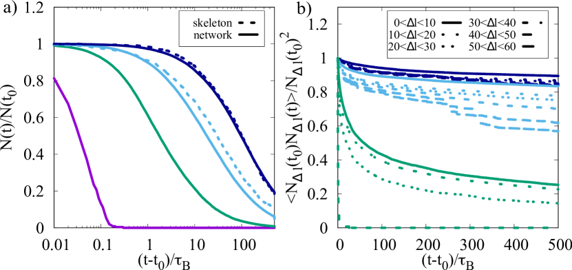
Figure 9: (a) Fractions of particles that stayed in contact until time $t$ given that they were in contact at time $t_{0}$. The colors indicate the strength of attraction as given in the legend in Fig. 6. For the gel networks the result is also shown for the cases where only particles in the reduced networks (skeleton) are considered. (b) Correlation functions similar to those in Fig. 8(a) where all real space distances $\Delta r$ are now replaced by network distances $\Delta l$, i.e., the number of colloids in the minimal path along particles in contact that connects the two considered colloids. The same colors as in Fig. 8(a) are used.

In Fig. 9(a) we show how many bonds between particles survive up to a time $t-t_{0}$. As expected, bonds are more stable in case of stronger attractions. Furthermore, in case of gel networks the bonds between particles of the reduced network (dashed lines) are more stable than bonds that occur anywhere (solid lines). Note that the differences between particles of the reduced network and all particles of the structure are more pronounced for intermediate attractions $\epsilon=9$ (light-blue) while they are small for the case of strong attractions $\epsilon=15$ (dark-blue).

III.3.2 Network correlations

While the analyzes of the previous subsection only acknowledges the rearrangements in space, we also want to explore changes of the network topology. Therefore, we consider the network distance $\Delta l$ between two particles that is defined as the number of particles in the minimal chain of particles in contact that connects the initial particle with the target particle. We calculate these distances for all pairs of particles by using the Floyd-Warshall algorithmfloyd ; warshall .

In the following we consider similar correlation functions as in the previous subsection but the real space distances $\Delta r$ are now replaced by network distances $\Delta l$. The resulting correlation functions are shown in Fig. 9(b). In the case of the cluster fluid with weak attractions $\epsilon=6.5$ the correlation function decays very fast, while for the gel networks with $\epsilon=9$ and $\epsilon=15$ the decay is slower. Note that while the spatial correlations in Fig. 8(a) were very similar for the two considered gel networks, the correlations with respect to the network topology in Fig. 9(b) differ significantly. The network topology of gel networks with $\epsilon=15$ is more stable than the one with $\epsilon=9$. That means once a suitable network configuration is found the reformation of the network structure in a network with large attraction strength is slower than for intermediate attractions. Note that as we will show in the following even small rearrangements in space can have a major impact on the network topology.

Figure 10: (a,b) Snapshots of a system with $\epsilon=15$, $\kappa=15$, and $\eta=0.05$ after 2500$\tau_{B}$ and 2600$\tau_{B}$. A new connection forms in the top of the pictures. (c) Number of particles that can be reached within $\Delta l$ steps along particles in contact from a randomly chosen starting particle. For visibility only curves for 30 randomly chosen starting particles are depicted. If all possible 2578 curves were shown they would lay dense. The brown curves are determined for the configuration after 2500$\tau_{B}$ depicted in (a) and the blue curves of the configuration after 2600$\tau_{B}$ shown in (b). The black lines show average curves (dashed for 2500$\tau_{B}$, solid for 2600$\tau_{B}$). Note that some lines for 2500$\tau_{B}$ are hidden behind the curves for 2600$\tau_{B}$. (d) Triangles: Full width at half maximum (FWHM) of the neighbor string plots as shown in (c) where now all possible curves are considered in the evaluation. Circles: Average number of steps needed to reach every particle in the network. Both quantities are plotted as a function of time. The connection event that is visible in the snapshots (a,b) leads to a jump of the shown quantities.

In Fig. 10 we depict how the appearance of a new connection influences the network topology. It is clearly visible that between the shown snapshots for $2500\tau_{B}$ and for $2600\tau_{B}$ a new connection is formed (encircled in black). If we calculate for each particle how many other particles can be reached in $k$ steps for a randomly chosen starting particles we find curves as plotted in Fig. 10(c). The range where these curves can be found indicates that the new connection makes the network more dense in the sense that a higher number of particles can be reached in less steps. To further quantify this result we calculate the average number of steps needed to reach the whole network and the full width at half maximum (FWHM) of the curves as in Fig. 10(c) as a function of time. Fig. 10(d) shows that between 2500$\tau_{B}$ and 2600$\tau_{B}$ these quantities jump to a lower value as expected because particles can be reached faster and the density of the network increases.

These rearrangements of connections - either new formation or destruction - also explain the small jumps that are visible in Fig. 9(b) for $\epsilon=9$. Here either new connections are formed or old connections are lost, such that big groups of particles do not anymore belong to the same network distance range because the topology of the network has changed dramatically.

III.3.3 Relation between network distance and spatial distance

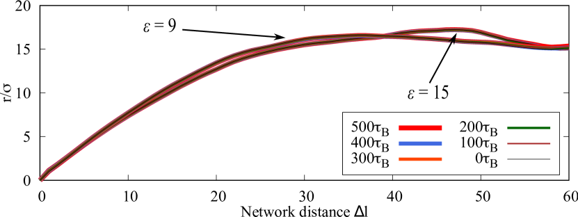
Figure 11: Spatial distance $\Delta r$ as a function of network distance $\Delta l$ for gel networks with $\epsilon=9$ and $\epsilon=15$. Otherwise, as always $\kappa=15$ and $\eta=0.05$. Ageing times after an initial thermalization of $3000\tau_{B}$ are depicted by the color. Note that for a given $epsilon$ the curves at different ageing times collapse almost perfectly. Results are averaged over 4 independent runs.

We analyze the relationship between network distance and spatial distance in gel networks. After an equilibration time of $3000\tau_{B}$ we start from the meta-stable state which is reached and calculate average spatial distance as a function of network distance. Fig. 11 shows the results for different ageing times after the initial relaxation. For a given $\epsilon$ the curves at different ageing times collapse almost perfectly indicating that the relation between network topology and location in space is hardly affected by the ageing process. Interestingly, there are differences for different attraction strengths: The spatial distance shows a maximal value which depends on the attraction strength. This indicates that for a large attraction of $\epsilon=15$ longer and thinner strands form such that more steps are needed to reach the same spatial distance. This finding is in agreement with the larger mesh size observed in Fig. 6.

IV Conclusion

Due to the competition of depletion attractions and longer-ranged repulsions between the colloidal particles in colloid-polymer mixtures, complex, heterogeneous structures can be observed for attractions that are stronger than at the binodal line of the fluid-liquid phase separation in equilibrium. Our Brownian dynamics simulations reveal significant differences between unpercolated cluster fluids, gel networks, and clumpy gels. While the dynamics of cluster fluids can be well described by free diffusion-like motion of the clusters, the dynamics of gel networks and bulky gels is much slower and does not reach a diffusive regime at the timescales that are accessible to simulations.

Our structural analyses demonstrate that there are large voids in gel networks. A typical length can be extracted resembling a mesh length. Furthermore, we introduce reduced networks where all particles are left out except for those that resemble the important connections between particles. The reduced networks can be employed to identify percolating strands and as an additional method to characterize the difference between gel networks and clumpy gels.

The observed gel-like structures are meta-stable and the perfect equilibrium states are actually still unknown (see also discussion in archer ). We observe and characterize the ageing dynamics in all gel-like states. We want to stress that different ageing processes can be observed on different length scales, e.g., neighbor particles can disconnect and connect again especially in case of smaller attractions. On a longer length scale, namely typically the mesh size, the strands of a gel network can slowly rearrange.

Concerning different gel networks, we find that correlations depending on the network topology decay much faster in case of small attraction then in case of strong attraction between the colloids. The reason for this difference are strands that can rupture for small attractions but hardly for strong ones. We observe that such rupture events do not have an significant impact on the structure in space or the decay times of spatial correlations. However, we expect that the rupture of strands might influence the mechanic stability or the shear slabs that occur under continuous shear kohl2 which will be the topic of future works.

Furthermore, in future we also want to explore the slowdown of the different types of dynamics in a gel network in more detail. In a clumpy gel at large densities the slowdown sometimes is attributed to a glass-like effective ergodicity breaking toledano ; zhang , we expect that that the different types of dynamics that occur in a gel network become arrested at different transitions. As we have related the ergodicity breaking transition of thermal jamming to a directed percolation in time milz ; maiti , we want to find out whether the step-wise dynamic arrest in gel networks also can be related to percolation transitions in time and how these are related to the percolation in space.

Data Availability Statement

The data that support the findings of this study are available from the corresponding author upon reasonable request.

- (1) B.V. Derjaguin and L. Landau, Theory of stability of highly charged lyophobic sols and adhesion of highly charged particles in solutions of electrolytes, Acta Physicochimica (USSR) 14, 633 (1941).
- (2) E.J. Verwey and J.T.G. Overbeek, Theory of the Stability of Lyophobic Colloids, Elsevier, Amsterdam (1948).
- (3) S. Asakura and F. Oosawa, On interaction between two bodies immersed in a solution of macromolecules, J. Chem. Phys. 22, 1255 (1954).
- (4) A. Vrij, Polymers at interfaces and interactions in colloidal dispersions. Pure and Appl. Chem. 48, 471 (1976).
- (5) K. Binder, P. Virnau, and A. Statt, Perspective: The Asakura Oosawa model: A colloid prototype for bulk and interfacial phase behavior, J. Chem. Phys. 141, 140901 (2014).
- (6) M. Edelmann and R. Roth, Gyroid phase of fluids with spherically symmetric competing interactions, Phys. Rev. E 93, 062146 (2016).
- (7) E.C. Oğuz, A. Mijailović, and M. Schmiedeberg, Self-assembly of complex structures in colloid-polymer mixtures, Phys. Rev. E 98, 052601 (2018).
- (8) N.A.M. Verhaegh, D. Asnaghi, H.N.W. Lekkerkerker, M. Giglio, and L. Cipelletti, Transient gelation by spinodal decomposition in colloid-polymer mixtures, Physica A 242, 104 (1997).
- (9) P.J. Lu, E. Zaccarelli, F. Ciulla, A.B. Schofield, F. Sciortino, and D.A. Weitz, Gelation of particles with short-range attraction, Nature 453, 499 (2008).
- (10) D. Richard, J. Hallett, T. Speck, and C.P. Royall, Coupling between criticality and gelation in "sticky" spheres: A structural analysis, Soft Matter 14, 5554 (2018).
- (11) D. Richard, C.P. Royall, and T. Speck, Communication: Is directed percolation in colloid-polymer mixtures linked to dynamic arrest?, J. Chem. Phys. 148, 241101 (2018).
- (12) J.H. Cho, R. Cerbino, and I. Bischofberger, Emergence of Multiscale Dynamics in Colloidal Gels, Phys. Rev. Lett. 124, 088005 (2020).
- (13) A.J. Archer and N.B. Wilding, Phase behavior of a fluid with competing attractive and repulsive interactions, Phys. Rev. E 76, 031501 (2007).
- (14) J.C. Fernandez Toledano, F. Sciortino, and E. Zaccarelli, Colloidal systems with competing interactions: from an arrested repulsive cluster phase to a gel, Soft Matter 5, 2390 (2009).
- (15) I. Zhang, C. P. Royall, M.A. Faers, and P. Bartlett, Phase separation dynamics in colloid–polymer mixtures: the effect of interaction range, Soft Matter 9, 2076 (2013).
- (16) E. Mani, W. Lechner, W.K. Kegel, and P.G. Bolhuis, Equilibrium and non-equilibrium cluster phases in colloids with competing interactions, Soft Matter 10, 4479 (2014).
- (17) M.E. Helgeson, Y. Gao, S.E. Moran, J. Lee, M. Godfrin, A. Tripathi, A. Bosee, and P.S. Doyleb, Homogeneous percolation versus arrested phase separation in attractively-driven nanoemulsion colloidal gels, Soft Matter 10, 3122 (2014).
- (18) M. Kohl, R.F. Capellmann, M. Laurati, S.U. Egelhaaf, and M. Schmiedeberg, Directed percolation identified as equilibrium pre-transition towards non-equilibrium arrested gelstates, Nature Communications 7, 11817 (2016).
- (19) J.M. van Doorn, J. Bronkhorst, R. Higler, T. van de Laar, and J. Sprakel, Linking Particle Dynamics to Local Connectivity in Colloidal Gels, Phys. Rev. Lett. 118, 188001 (2017).
- (20) M. Kohl and M. Schmiedeberg, Shear-induced slab-like domains in a directed percolated colloidal gel, Eur. Phys. J. E 40, 71 (2017).
- (21) L. Milz and M. Schmiedeberg, Connecting the random organization transition and jamming within a unifying model system, Phs. Rev. E 88, 062308 (2013).
- (22) M. Maiti and M. Schmiedeberg, Ergodicity breaking transition in a glassy soft sphere system at small but non-zero temperatures, Scientific Reports 8, 1837 (2018).
- (23) M. P. Allen and D. J. Tildesley, Computer simulations of liquids, Oxford University Press, New York (1990).
- (24) R. W. Floyd, Algorithm 97 (SHORTEST PATH), Communications of the ACM 5, 345 (1962).
- (25) S. Warshall, A Theorem on Boolean Matrices, Journal of the ACM 9, 11 (1962).