The Quasar Feedback Survey: Discovering hidden Radio-AGN and their connection to the host galaxy ionised gas

Abstract

We present the first results from the Quasar Feedback Survey, a sample of 42 $z<0.2$, [O iii] luminous AGN ($L_{\rm[O~{}III]}>10^{42.1}$ ergs s^-1) with moderate radio luminosities (i.e. $L_{\rm 1.4GHz}>10^{23.4}$ W Hz^-1; median $L_{\rm 1.4GHz}=5.9\times 10^{23}$ W Hz^-1). Using high spatial resolution ($\sim$0.3–1 arcsec), 1.5–6 GHz radio images from the Very Large Array, we find that 67 percent of the sample have spatially extended radio features, on $\sim$1–60 kpc scales. The radio sizes and morphologies suggest that these may be lower radio luminosity versions of compact, radio-loud AGN. By combining the radio-to-infrared excess parameter, spectral index, radio morphology and brightness temperature, we find radio emission in at least 57 percent of the sample that is associated with AGN-related processes (e.g. jets, quasar-driven winds or coronal emission). This is despite only 9.5–21 percent being classified as radio-loud using traditional criteria. The origin of the radio emission in the remainder of the sample is unclear. We find that both the established anti-correlation between radio size and the width of the [O iii] line, and the known trend for the most [O iii] luminous AGN to be associated with spatially-extended radio emission, also hold for our sample of moderate radio luminosity quasars. These observations add to the growing evidence of a connection between the radio emission and ionised gas in quasar host galaxies. This work lays the foundation for deeper investigations into the drivers and impact of feedback in this unique sample.

1 Introduction

Active galactic nuclei (AGN) are amongst the most powerful phenomena in the observable universe and are generally accepted to inject significant energy into the gas in galaxies and the intergalactic medium and, consequently, play a vital role in galaxy evolution (e.g. see reviews in Alexander & Hickox, 2012; Fabian, 2012; King & Pounds, 2015). Over time our understanding of the physical processes in and around AGN has grown immensely. However, important questions remain unanswered.

For AGN with powerful radio jets, particularly those with low accretion rates residing in massive galaxies in the local Universe, there is compelling evidence that AGN are able to regulate star formation through the jets injecting energy into the gaseous halos and regulating the cooling of gas onto the galaxy (e.g. see review in McNamara & Nulsen, 2012; Hardcastle & Croston, 2020). On the other hand, there are many debated topics in the literature concerning radiatively efficient AGN such as quasars, which we define here as Type 1 or Type 2 AGN with bolometric luminosities of $L_{\rm AGN}\gtrsim 10^{45}$ erg s^-1 (e.g. see review in Harrison, 2017). For example, there is a significant debate about the dominant processes that produce the radio emission in typical ‘radio-quiet’ AGN and through which mechanisms these AGN transfer energy to their host galaxies (e.g. Zakamska et al., 2016a; Kellermann et al., 2016; Wylezalek & Morganti, 2018; Panessa et al., 2019; Jarvis et al., 2019). Furthermore, the details of exactly how, or indeed if, these AGN impact upon the evolution of their host galaxies remains controversial and uncertain (e.g. Husemann et al., 2016; Villar-Martín et al., 2016; Maiolino et al., 2017; Harrison, 2017; Cresci & Maiolino, 2018; Perna et al., 2018; Rosario et al., 2018; Baron et al., 2018; Scholtz et al., 2018, 2020; do Nascimento et al., 2019; Brownson et al., 2020; Yesuf & Ho, 2020; Greene et al., 2020; Bluck et al., 2020; Bischetti et al., 2020). Building a multi-wavelength quasar survey to address these questions is the focus of the Quasar Feedback Survey, which we introduce here.

The origin of the radio emission in the majority of AGN (i.e. those without powerful relativistic radio jets and that typically have radio luminosities $L_{\textrm{1.4GHz}}\lesssim 10^{25}$ W Hz^-1) is widely debated and is the main focus of this paper. On one hand, the radio emission could be dominated by synchrotron emission caused by shocks from exploding supernovae and hence be directly related to the star formation in the host galaxy (see e.g. Condon, 1992; Bonzini et al., 2013; Condon et al., 2013; Padovani et al., 2015). Alternatively, the majority of the radio emission could originate from the AGN (see e.g. Padovani, 2017; Jarvis et al., 2019). The three most likely ways in which AGN can generate radio emission are: i) synchrotron emission from jets (Kukula et al., 1998; Kharb et al., 2015, 2017), ii) coronal emission (Laor & Behar, 2008; Behar et al., 2018) and iii) synchrotron from electrons accelerated at non-relativistic shocks that may result from wide angle sub-relativistic quasar winds (Nims et al., 2015; Zakamska et al., 2016a), with magnetocentrifugal winds (Blandford & Payne, 1982; Everett, 2005; Fukumura et al., 2010), thermally driven AGN winds (Begelman & McKee, 1983; Woods et al., 1996; Mizumoto et al., 2019) or any combination of the above also being possibilities. In this paper we identify sources in the Quasar Feedback Survey sample where AGN processes contribute significantly to the radio emission, and do not attempt to distinguish between the different AGN-related mechanisms.

Multiple studies of local and low-redshift AGN ($z<0.8$) have shown that the level of radio emission in AGN host galaxies is strongly connected to the presence of ionised outflows, which have primarily been identified through broad and asymmetric [O iii] emission lines (see e.g. Heckman et al., 1981; Wilson & Heckman, 1985; Veilleux, 1991; Whittle, 1992; Nelson & Whittle, 1996; O’Dea, 1998; Holt et al., 2008; Kim et al., 2013; Mullaney et al., 2013; Zakamska & Greene, 2014; Villar Martín et al., 2014; Santoro et al., 2020). Across these studies, this observation holds for a wide range of AGN luminosities (i.e. Seyferts and quasars) and orders of magnitude in radio luminosity (i.e. from typical ‘radio-quiet’ AGN through to the most luminous ‘radio-loud’ AGN). Nonetheless, some other studies, which used emission-line selected samples, have suggested that other factors (e.g. Eddington ratio and stellar mass) may be more important than the level of radio emission in determining the prevalence and properties of ionised outflows (e.g. Wang et al., 2018; Rakshit & Woo, 2018a; Kauffmann & Maraston, 2019). However, these studies are all based upon spatially unresolved data, and a more direct connection between radio emission can be observed when using spatially-resolved information. For example, Molyneux et al. (2019) finds that extreme [O iii] outflows (FWHM $>$ 1000 km s^-1) are more prevalent when the projected size of the radio emission is within, as opposed to extending beyond, the SDSS spectroscopic fibre (where the [O iii] line width is measured). We further investigate the relationship between radio emission and ionised gas in this work.

We present multi-frequency radio observations of the 42 sources in the Quasar Feedback Survey, which we use in combination with archival data to identify sources where radio emission is associated with the AGN rather than star formation and to explore the radio – outflow connection. In Section 2, we describe the survey and present the sample selection. In Section 3 we describe our Karl G. Jansky Very Large Array (VLA) data, its reduction and imaging. Section 4 presents our results, which we then discuss in Section 5. We summarise our conclusions in Section 6. In the supplementary material we provide figures showing all of the images used in this work, a summary of our observations for each target and a description of the relevant literature work on each target (Appendix A and B).

We adopt $H_{0}=70$ km s^-1 Mpc^-1, $\Omega_{M}=0.3$, $\Omega_{\Lambda}=0.7$ throughout, and define the radio spectral index, $\alpha$, using $S_{\nu}\propto\nu^{\alpha}$. We assume a Chabrier (2003) initial mass function (IMF).

2 Survey Description

In this paper we present the first results from our Quasar Feedback Survey, which is designed to study the spatially-resolved multi-wavelength properties of relatively low redshift ($z<0.2$) quasar host galaxies identified based on their optical emission lines. The main survey goals are to investigate: (1) the origin of radio emission; (2) the properties of multi-phase outflows and; (3) the impact that quasars have on their host galaxies.

2.1 Pilot Studies Summary

The Quasar Feedback Survey builds upon a series of papers where we presented pilot observations on a smaller sample, which were pre-selected to be quasars that were expected to host powerful ionised outflows based upon their SDSS spectra (i.e. [O iii] emission-line components with full width half maximum – FWHM $>$ 700 km s^-1; see Fig. 1; Harrison et al. 2014; Harrison et al. 2015; Jarvis et al. 2019). This sample consisted of ten AGN, nine of which are part of this Quasar Feedback Survey and all of which are ‘radio-quiet’ based on the Xu et al. (1999) definition (see Section 2.4). We used spatially resolved radio observations and IFS data to find kiloparsec-scale radio features, galaxy wide ionised gas outflows, and signatures of jet–gas interactions. In Jarvis et al. (2019) we demonstrated that radio emission originating from the AGN can be effectively identified by combining spatially resolved radio observations and an observed radio excess beyond what is predicted from the radio–infrared (IR) correlation for star-forming galaxies. In this work, we expand upon Jarvis et al. (2019) by increasing our sample of sources with high resolution radio images by a factor of 4 (see Section 2.2).

In Jarvis et al. (2020) we studied the CO emission and ultraviolet (UV) – far infrared (FIR) spectral energy distributions (SEDs) for the nine Quasar Feedback Survey pilot targets. We found that, for at least seven of the targets, the host galaxies had high molecular gas fractions and short depletion times, which are consistent with those expected for the overall galaxy population with matched stellar masses and specific star formation rates. This is despite the presence of powerful quasars and ionised outflows in these sources. This work suggested that the AGN do not have an immediate appreciable impact on the global molecular gas content, but does not rule out a smaller scale impact over longer timescales. Finally, in Lansbury et al. (2018) we studied the X-ray emission in one of our survey targets, J1430+1339 (nicknamed the “Teacup AGN”; see Appendix Supporting Information), investigating both the X-ray emission from the nucleus and the spatially-resolved X-rays, which we found to be co-spatial with bubbles of radio and emission-line gas.

In the following sub-section we describe the target selection for the wider Quasar Feedback Survey sample presented in this work. Importantly, unlike the pilot studies described above, there is no selection criterion based on the width of the [O iii] line (see Fig. 1), and hence no explicit pre-selection on the presence or properties of AGN-driven ionised outflows.

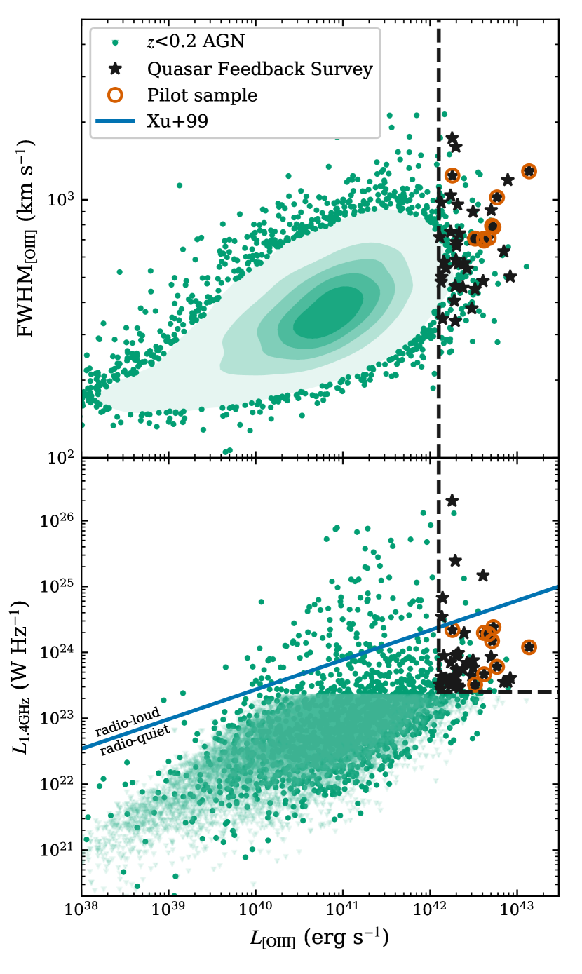
Figure 1: The basic properties of the 42 sources in the Quasar Feedback Survey (black stars; see Table 1) and the criteria used to select them (black dashed lines) compared to the overall Mullaney et al. (2013) $z<0.2$ AGN population plotted as green circles and density contours. The sources in our pilot studies (e.g. Jarvis et al., 2019) are marked with red circles in addition to the black stars denoting their membership in the Quasar Feedback Survey sample. Top: The flux-weighted average FWHM from the Mullaney et al. (2013) two Gaussian [O iii]$\lambda 5007$ line fits versus the total observed [O iii] luminosity. Bottom: the 1.4 GHz radio luminosity from NVSS versus the total observed [O iii] luminosity (AGN with upper limits on their radio luminosity are shown as pale green triangles). The blue line marks the division between ‘radio-loud’ and ‘radio-quiet’ AGN from Xu et al. (1999), and the majority (37/42) of our quasars are classified as radio-quiet using this criterion.

2.2 Target selection

The targets presented in this work were selected from the parent sample of $\sim$24 000 $z<0.4$ spectroscopically identified AGN from the Sloan Digital Sky Survey (SDSS) presented in Mullaney et al. (2013). We note that we re-calculated the relevant luminosities using the cosmological parameters adopted for this current paper.

We restricted the table from Mullaney et al. (2013) to the 17 431 sources with a redshift of $z<0.2$. This redshift cut was designed to provide a sample of tens of powerful AGN with quasar-like luminosities (i.e. $L_{\rm AGN}\gtrsim 10^{45}$ erg s^-1; see below) whilst selecting galaxies that are still at low enough redshift to be studied with kiloparsec-scale resolution or better. Specifically, a typical range of resolutions that we expect from our high resolution multi-wavelength imaging will be approximately 0.2–0.7 arcsec (see pilot studies in Harrison et al., 2014; Harrison et al., 2015; Jarvis et al., 2019), which corresponds to 0.2–0.7 kpc and 0.7–2.3 kpc at the lowest redshift ($z=0.05$) and highest redshift ($z=0.2$) of the sample, respectively.

We then restricted this $z<0.2$ AGN sample to the 220 targets with the highest [O iii]$\lambda 5007$ luminosities, specifically those with $L_{\rm[O~{}III]}>10^{42.11}$ ergs s^-1 calculated using the total flux values from the two Gaussian fits from Mullaney et al. (2013). This cut enabled us to select AGN with quasar level luminosities (e.g. Reyes et al., 2008, see Section 2.3). For the last primary selection criterion for our initial sample, we selected the 67 quasars with a radio luminosity of $L_{\rm 1.4GHz}>10^{23.45}$ W Hz^-1 (see Fig. 1 and Table 1). For this selection, we used the K-corrected radio luminosity values derived from the 1.4 GHz flux densities from NRAO VLA Sky Survey (NVSS; Condon et al., 1998) as matched in Mullaney et al. (2013). Our chosen radio luminosity cut was motivated to be above the NVSS detection limit (see Fig. 1), where we, consequently, have a more robust understanding of the connection between the ionised gas properties and radio properties of the underlying population (e.g. Mullaney et al., 2013; Molyneux et al., 2019).

The final sample consists of all 42 remaining sources with a right ascension of 10 $<$ RA $<$ 300 degrees and a declination of 24 $<$ Dec or Dec $>$ 44 degrees. These sky position criteria were chosen to help facilitate observational scheduling at the VLA.

Based on the optical spectra of our targets, 25 are Type 2 AGN (60 percent) and the other 17 (40 percent) are Type 1 (broad line) AGN. We show the SDSS spectra for our targets in Fig. 2 (for J1553$+$4407) and Figs Supporting Information – Supporting Information (for the other 41 targets). In Table 1 we list all 42 targets with their sky positions, redshifts and AGN Type.

Several of our targets have been the subject of multi-wavelength studies in the literature. We summarise the most relevant of these studies for each of the targets in Appendix Supporting Information and, where relevant, we draw on this previous knowledge of these targets to aid with the analyses and discussion in this work.

Table 1: The Quasar Feedback Survey sources and their basic properties. (1) Source name; (2)–(3) Optical RA and Dec positions from SDSS (DR7) in the format hh:mm:ss.ss for RA and dd:mm:ss.s for Dec; (4) Redshift of the source from SDSS (DR7); (5) Rest-frame 1.4 GHz radio luminosities from NVSS using a spectral index of $\alpha=-0.7$ and assuming $S_{\nu}\propto\nu^{\alpha}$. The typical log errors are $\sim$0.03; (6) 1.4 GHz flux density of the target from NVSS; (7) Total observed [O iii]$\lambda 5007$ luminosity calculated using the fluxes from Mullaney et al. (2013), the typical log errors are $\sim$0.01; (8) Flux-weighted average of the FWHM from the Mullaney et al. (2013) two Gaussian fits to the [O iii] line profile; (9) AGN Type based on the width of the H$\alpha$ line from SDSS DR7 spectra from Mullaney et al. (2013), with 1 for broad line (Type 1) and 2 for narrow line (Type 2).
^† These nine sources have been previously studied by our group (see e.g. Harrison et al., 2014; Jarvis et al., 2019, 2020, Fig, 1).
^∗ This source has also been published as 4C+54.27.
^†† This source has also been published as Mrk783.
^‡ This source has also been published as PKS1345+12 and 4C12.50.

Name	RA	Dec	$z$	log($L_{\textrm{1.4GHz}}$)	$S_{\textrm{1.4GHz}}$	log($L_{\textrm{[O~{}{\sc iii}]}}$)	FWHM${}_{\textrm{[O~{}{\sc iii}]}}$	AGN type
	(J2000)	(J2000)		(/W Hz-1)	(mJy)	(/erg s-1)	(km s-1)
(1)	(2)	(3)	(4)	(5)	(6)	(7)	(8)	(9)
J0749+4510	07:49:06.50	+45:10:33.9	0.192	25.2	147.1$\pm$5.1	42.61	484$\pm$16	1
J0752+1935	07:52:17.84	+19:35:42.2	0.117	23.9	24.9$\pm$0.9	42.70	913$\pm$26	1
J0759+5050	07:59:40.96	+50:50:24.0	0.055	23.5	44.9$\pm$1.4	42.32	958$\pm$19	2
J0802+4643	08:02:24.35	+46:43:00.6	0.121	23.5	8.9$\pm$0.5	42.11	716$\pm$20	2
J0842+0759	08:42:05.57	+07:59:25.5	0.134	23.9	16.6$\pm$1.0	42.49	899$\pm$15	1
J0842+2048	08:42:07.50	+20:48:40.1	0.181	23.5	3.6$\pm$0.4	42.24	752$\pm$34	1
J0907+4620	09:07:22.36	+46:20:18.0	0.167	24.5	47.1$\pm$1.5	42.13	502$\pm$31	2
J0909+1052	09:09:35.49	+10:52:10.5	0.166	23.6	6.0$\pm$0.5	42.28	406$\pm$17	2
J0945+1737†	09:45:21.33	+17:37:53.2	0.128	24.3	45.6$\pm$1.4	42.67	711$\pm$12	2
J0946+1319	09:46:52.57	+13:19:53.8	0.133	23.6	7.9$\pm$0.5	42.89	1193$\pm$26	1
J0958+1439†	09:58:16.88	+14:39:23.7	0.109	23.5	10.9$\pm$0.5	42.52	707$\pm$33	2
J1000+1242†	10:00:13.14	+12:42:26.2	0.148	24.3	34.8$\pm$1.1	42.62	706$\pm$16	2
J1010+0612†	10:10:43.36	+06:12:01.4	0.098	24.3	92.4$\pm$3.3	42.26	1241$\pm$30	2
J1010+1413†	10:10:22.95	+14:13:00.9	0.199	24.1	11.1$\pm$0.5	43.14	1289$\pm$18	2
J1016+0028	10:16:53.82	+00:28:57.1	0.116	23.6	11.8$\pm$0.9	42.18	543$\pm$16	2
J1016+5358	10:16:23.76	+53:58:06.1	0.182	23.5	3.2$\pm$0.5	42.13	976$\pm$39	2
J1045+0843	10:45:05.16	+08:43:39.0	0.125	23.8	17.6$\pm$1.2	42.42	541$\pm$30	1
J1055+1102	10:55:55.34	+11:02:52.2	0.145	23.5	5.7$\pm$0.4	42.52	451$\pm$16	2
J1100+0846†	11:00:12.38	+08:46:16.3	0.100	24.2	59.8$\pm$1.8	42.71	793$\pm$16	2
J1108+0659	11:08:51.03	+06:59:01.4	0.181	24.0	11.1$\pm$0.5	42.32	566$\pm$11	2
J1114+1939	11:14:23.81	+19:39:15.8	0.199	24.0	8.4$\pm$0.5	42.30	584$\pm$19	2
J1116+2200	11:16:25.34	+22:00:49.3	0.143	23.7	10.5$\pm$0.5	42.38	457$\pm$18	2
J1222-0007	12:22:17.85	-00:07:43.7	0.173	23.6	4.5$\pm$0.4	42.85	631$\pm$37	2
J1223+5409∗	12:23:13.21	+54:09:06.5	0.156	25.4	387.6$\pm$11.6	42.29	339$\pm$11	1
J1227+0419	12:27:39.83	+04:19:32.4	0.180	23.8	6.8$\pm$0.5	42.49	701$\pm$23	1
J1300+0355	13:00:07.99	+03:55:56.5	0.184	24.3	21.6$\pm$0.8	42.39	568$\pm$10	1
J1302+1624††	13:02:58.83	+16:24:27.7	0.067	23.5	32.9$\pm$1.1	42.29	463$\pm$28	1
J1316+1753†	13:16:42.90	+17:53:32.5	0.150	23.8	10.3$\pm$0.5	42.77	1022$\pm$28	2
J1324+5849	13:24:18.25	+58:49:11.6	0.192	23.8	7.1$\pm$0.5	42.24	1040$\pm$72	1
J1347+1217‡	13:47:33.36	+12:17:24.3	0.121	26.3	5397.2$\pm$161.9	42.25	1730$\pm$35	2
J1355+2046	13:55:50.20	+20:46:14.5	0.196	23.6	4.2$\pm$0.5	42.30	1605$\pm$59	1
J1356+1026†	13:56:46.10	+10:26:09.0	0.123	24.4	62.9$\pm$1.9	42.73	783$\pm$6	2
J1430+1339†	14:30:29.88	+13:39:12.0	0.085	23.7	26.5$\pm$0.9	42.62	695$\pm$25	2
J1436+4928	14:36:07.21	+49:28:58.5	0.128	23.6	9.4$\pm$0.9	42.16	572$\pm$30	2
J1454+0803	14:54:34.35	+08:03:36.7	0.130	23.7	12.7$\pm$0.6	42.30	664$\pm$20	1
J1509+1757	15:09:13.79	+17:57:10.0	0.171	24.0	11.8$\pm$0.5	42.30	685$\pm$26	1
J1518+1403	15:18:56.27	+14:03:19.0	0.139	23.6	8.6$\pm$0.9	42.13	481$\pm$25	2
J1553+4407	15:53:15.94	+44:07:49.3	0.197	23.6	4.2$\pm$0.5	42.48	379$\pm$14	2
J1555+5403	15:55:01.44	+54:03:26.9	0.180	23.5	3.4$\pm$0.5	42.33	741$\pm$52	1
J1655+2146	16:55:51.37	+21:46:01.8	0.154	23.6	6.6$\pm$0.5	42.92	504$\pm$27	1
J1701+2226	17:01:58.24	+22:26:41.9	0.197	24.8	64.0$\pm$2.6	42.14	346$\pm$5	1
J1715+6008	17:15:44.05	+60:08:35.6	0.157	23.9	13.8$\pm$0.6	42.16	576$\pm$8	2

2.3 Our sample in context

In Table 1 we present the radio luminosities and [O iii] luminosities of our sample which are visually presented in the context of the parent population in Fig. 1. Our [O iii] luminosity cut of $L_{\rm[O~{}III]}>10^{42.11}$ ergs s^-1 represents the 1.3 percent most luminous targets from the parent sample within our redshift range of interest (i.e. $z<0.2$). The [O iii] luminosity range of our targets (i.e. $L_{\rm[O~{}III]}=10^{42.1}$–$10^{43.1}$ ergs s^-1) corresponds to an AGN luminosity of $L_{\rm AGN}=10^{45.6}$–$10^{46.6}$ erg s^-1, assuming a bolometric correction of 3500 (Heckman et al., 2004). Since it is known that [O iii] often over-predicts the AGN luminosity by about an order of magnitude (Schirmer et al., 2013; Hainline et al., 2013) this roughly corresponds to a cut of $L_{\rm AGN}\gtrsim 10^{45}$ erg s^-1, which can be verified using optical–far infrared SED analyses (e.g. Jarvis et al., 2019, 2020). The range of luminosities covered by our sample is designed to be representative of typical AGN luminosities found during the peak epoch of cosmic black hole growth. Specifically, the knee of the bolometric AGN luminosity function is $L_{\rm AGN}=10^{45.8}$ erg s^-1 at $z=0.8$ and $L_{\rm AGN}=10^{46.6}$ erg s^-1 at $z=2$, following Shen et al. (2020) (see also Hopkins et al. 2007), which overlap with the AGN luminosities in this sample.

In Table 1 we also give the flux-weighted average of the FWHM of the two [O iii] emission-line Gaussian components as fit by Mullaney et al. (2013). These values for our full sample are represented in Fig. 1, compared to the parent sample, where it can be seen that these emission-line widths are representative of the parent sample with FWHM values spanning 340–1730 km s^-1. Sampling the full range in [O iii] emission-line profiles is a crucial step forward for our wider Quasar Feedback Survey presented here, compared to our previous work that focused on sources with broad [O iii] line widths (e.g. Harrison et al., 2014; Jarvis et al., 2019, see Section 2.1). In Fig. 2 (for J1553$+$4407) and Figs Supporting Information–Supporting Information we show zoom-ins of the [O iii] emission-line profile for each source revealing the broad diversity in profiles across the sample. This includes narrow and symmetric profiles (e.g. Fig. Supporting Information), double peaked profiles (e.g. Fig. Supporting Information) and broad asymmetric profiles (e.g. Fig. Supporting Information).

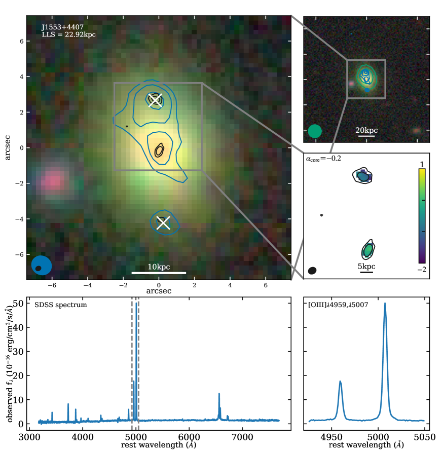
Figure 2: This figure highlights the observed properties of J1553$+$4407 and the data used in this paper; similar figures for the entire sample are shown in Appendix Supporting Information. In the upper left is an rgb image from the DESI Legacy Imaging Survey in the (z,r,g) bands, with contours from our VLA L-band data (1.5 GHz; $\sim$1 arcsec resolution; MR image) in blue and our C-band data (6 GHz; $\sim$0.3 arcsec resolution; HR image) in black. North is up and east is to the left. In the top right is a zoom-out with FIRST survey radio contours overlaid (green; 1.4 GHz; $\sim$5 arcsec resolution; LR image) in addition to the L-band (MR) contours in blue. The white X’s mark the radio peaks used to calculate the size for this source in Table 2 (in this case using the L-band [MR] data; see Section 4.1 for details). The middle right panel shows a zoom-in with the in-band spectral index map (colour bar inset to the right) from our C-band data (i.e. 4–8 GHz), with flux density contours (as to the left) overlaid. The value measured for the core spectral index (i.e. $\alpha_{\textrm{core}}$; see Section 4.3) is given in the top left of this panel. Radio contours for all data are plotted at levels of $\pm$[4, 8, 16, 32, 64, 128]$\sigma$ with dashed lines for the negative contours (in this case there are no negative features with at least $4\sigma$ significance). The beams for the relevant radio images are shown in the bottom left of each sub-plot in the matching colours. The bottom row shows the SDSS spectrum of the source with vertical grey dashed lines marking the region of the [O iii] doublet for which a zoom-in is shown to the right (the y-axis for both spectra is the same).

Our survey compliments several other ongoing and previous observational campaigns that also aim to study the drivers of ionised outflows and the broader impact of bolometrically luminous AGN (including quasars) on their host galaxies. We focus our comparison on surveys that aim to study the [O iii] emission because this was the basis of our sample selection (see Fig. 1).

At higher redshifts (i.e. larger than about 0.4–4.0) there are large IFS studies of powerful radio galaxies (Nesvadba et al., 2017) and X-ray selected AGN (Harrison et al., 2016; Circosta et al., 2018) as well as a number of smaller studies of the spatially-resolved gas kinematics in luminous AGN (e.g. Harrison et al., 2012; Liu et al., 2013; Liu et al., 2014; Carniani et al., 2015; Perna et al., 2015; Brusa et al., 2015; Kakkad et al., 2016; Zakamska et al., 2016b; Vietri et al., 2018). The advantage of studying sources at high redshift is that they cover the peak epoch of cosmic black hole growth, and, consequently there are a larger number of powerful sources where the impact of AGN/quasars might be most important (e.g. Hopkins et al., 2007; McCarthy et al., 2011). However, although advantages can be gained by the use of adaptive optics (e.g. Fischer et al., 2019; Davies et al., 2020b; Kakkad et al., 2020), it is typically not possible to reach kiloparsec-scale resolution observations at high redshift. The exception is by studying rare gravitationally lensed AGN host galaxies (e.g. Fischer et al., 2019; Chartas et al., 2020). The strong effect of surface brightness dimming also makes it very observationally expensive to study high redshift targets in comparable detail to their lower redshift counterparts. This is a very important consideration; for example, the faint radio emission associated with ‘radio-quiet’ AGN and quasars can be extended on sub-kiloparsec scales and the kinematic signatures of outflows can be hard to disentangle from host galaxy dynamics without high spatial resolution and high signal-to-noise ratio data (e.g. Jarvis et al., 2019; Venturi et al., 2018).

By studying AGN in the very local Universe (i.e. $z\lesssim 0.05$), excellent spatial resolution and sensitivity can be achieved. There are many spatially-resolved studies investigating ionised, and multi-phase, outflows from samples of local galaxies hosting AGN (e.g. Husemann et al., 2017; Ramakrishnan et al., 2019; Mingozzi et al., 2019; Schönell et al., 2019; Wylezalek et al., 2020; Davies et al., 2020a; Venturi et al., 2020). However, these surveys are naturally dominated by lower power AGN than our survey where we aim to focus on powerful quasars.

Overall, by focusing on sources at $z\approx 0.1$, our survey allows for both a reasonable spatial resolution ($\sim$1 kpc) and sensitivity, whilst also allowing us to build up a sample of bolometrically luminous AGN (also see e.g. Husemann et al., 2013; Karouzos et al., 2016; Rupke et al., 2017; Rose et al., 2018; Rakshit & Woo, 2018b; Balmaverde et al., 2020; Santoro et al., 2020). Importantly, we have selected our quasars from a well studied parent sample (Section 2.2) and, as is usually not the case for bolometrically luminous ‘radio-quiet’ quasars, we will start with a detailed study of the spatially-resolved radio properties.

2.4 Defining the targets as radio-loud or radio-quiet

The majority (37/42) of the Quasar Feedback Survey sample are ‘radio-quiet’ as defined by the [O iii] and radio luminosity division of Xu et al. (1999) (see Fig. 1). These classifications are tabulated in Table 2. This fraction of 88 percent ‘radio-quiet’ in our sample, is consistent with the ‘radio-quiet’ fraction of the overall AGN population (i.e. $\sim$90 percent; Zakamska et al., 2004).

We use the criterion of Xu et al. (1999) as our primary definition of ‘radio-quiet’ because it can be applied to both the Type 1 and Type 2 AGN in our sample. However, for the Type 1 sources we additionally consider the commonly used radio-loudness parameter $R$: the ratio of radio to optical brightness (Kellermann et al., 1989). Specifically, we follow the prescription of Ivezić et al. (2002) which calculates $R$ using the radio flux density at 1.4 GHz and the SDSS i band magnitude. We calculate $R$ using:

$$R=0.4(m_{i}-t),$$ (1)

where $m_{i}$ is the i band magnitude from SDSS DR16 (Ahumada et al., 2020) using either the de Vaucouleurs or exponential profile fits to the galaxy luminosity profile (whichever provides a better fit) and $t$ is the ‘AB radio magnitude’ calculated using:

$$t=-2.5\log\left(\frac{S_{\textrm{1.4GHz}}}{3631\textrm{Jy}}\right),$$ (2)

where $S_{\textrm{1.4GHz}}$ is the NVSS flux density as tabulated in Table 1. Of the 17 Type 1 AGN in our sample, we find that seven would be classified as radio-loud, with $R>1.0$. This includes the three Type 1 AGN that were also radio-loud following the Xu et al. (1999) criterion. We note that the four Type 1 targets, which did not meet the Xu et al. (1999) criterion, but with $R>1.0$ have extremely modest values of $1.1\leq R\leq 1.4$ and three additional sources lie right on the boundary with $R=1$. This is compared to the typical $R$ value for radio-loud sources from Ivezić et al. (2002) of 2.8. The sources in our sample which meet both ‘radio-loud’ criteria have values of $R=1.9$–2.5. The values of $R$ calculated for all of the Type 1 sources in our sample are tabulated in Table 2.

This result is consistent with recent works finding an overlap in the $R$ parameters measured for Seyfert galaxies and FRI radio galaxies, suggesting that these form a continuous population (Kharb et al., 2014). Our work demonstrates that this also extends to the most bolometrically luminous AGN.

The majority of this paper is dedicated to employing more physically motivated tests to establish how many of the ‘radio-quiet’ sources also have radio emission associated with the AGN, which we refer to as ‘Radio-AGN’ to distinguish from the more traditional ‘radio-loud’ and ‘radio-quiet’ divisions.

3 Observations and data reduction

We observed our entire sample with the VLA to produce spatially resolved radio maps with around 1 and 0.3 arcsec resolution at 1.5 and 6 GHz, respectively. The VLA data for nine of the sample have previously been presented in Jarvis et al. (2019) (highlighted in Table 1; see also Harrison et al., 2015). These observations were taken under proposal ID. 13B-127 [PI. Harrison], with observations carried out between 2013 December 1 and 2014 May 13 in four configuration – frequency combinations: (1) A-array in L-band (1–2 GHz; $\sim$1.0 arcsec resolution); (2) A-array in C-band (4–8 GHz; $\sim$0.3 arcsec resolution); (3) B-array in L-band (1–2 GHz; $\sim$4.0 arcsec resolution) and (4) B-array in C-band (4–8 GHz; $\sim$1.0 arcsec resolution). For more details about these observations and the reduction of these data see Jarvis et al. (2019).

The remainder of the sample were observed under proposal ID. 18A-300 [PI. Jarvis] using the A-array in the L- and C-bands (around 1.0 and 0.3 arcsec resolution at 1–2 and 4–8 GHz, respectively), and were observed between 2018 March 2 – 22. We observed for 7.1 hours in the L-band (5–10 minutes per source) and 9.5 hours in C-band (5–25 minutes per source). To improve the uv coverage, each source was observed in at least two scans spread across the 1–2 hour observing blocks. We began each observing block with a $\sim$10 minute scan of a standard calibration source (3C147, 3C286 or 3C138). We performed 3 minute scans (including slew-time) of nearby (typically within 10^∘) phase calibrators every 10–15 minutes. The details of the VLA observations for each source (phase calibrator and observation date) are given in Appendix Supporting Information.

3.1 Data reduction and imaging

We reduced and imaged the VLA 18A-300 data using casa version 5.1.2-4. Specifically, we used the VLA casa Calibration Pipeline default VLA recipe for Stokes I continuum. We then split each of the science targets into their own measurement set using 3 s time binning. To remove radio frequency interference from the L-band data (where it is stronger than in the C-band), we then used the casa task ‘flagdata’ in ‘tfcrop’ mode to apply additional flags to each L-band measurement set. After inspecting the pipeline calibrated data, we performed additional manual flagging of bad data using the casa tool ‘plotms’ for the C-band observations of J1045$+$0843 and J1108$+$0659, specifically flagging all of the data from antenna 6 in the first scan of each source.

To provide consistent analysis with the remainder of the sample, we re-imaged the VLA 13B-127 data for this work, rather than using the images which were created for Jarvis et al. (2019). In order to take into account the broad and varying bandwidths of our observations, all of the VLA images we present were made using the Multi-Frequency Synthesis (MFS) mode of the ‘clean’ function. We weighted the baselines using the Briggs weighting scheme with a robustness parameter of 0.5 (Briggs, 1995). For the C-band data we performed this imaging using two Taylor terms to model the frequency dependence of the sky emission in order to simultaneously generate in-band (i.e. 4–8 GHz) spectral index maps as well as maps depicting the reliability of the spectral index. The details of the new VLA images presented in this work (noise and beam size) are given in Appendix Supporting Information. All of these images, together with cutouts from the VLA ‘Faint Images of the Radio Sky at Twenty-cm’ survey (FIRST; Becker et al., 1995) and archival optical images from the Dark Energy Spectroscopic Instrument (DESI) Legacy Imaging Survey in the (z,r,g) bands (Dey et al., 2019) are shown in Appendix Supporting Information.

Throughout this work we use three sets of images for each source which we refer to as low resolution (LR), medium resolution (MR) and high resolution (HR) throughout, defined as:

• LR: We used 2 arcmin cutouts from FIRST to characterise the low resolution ($\sim$5 arcsec; 1.4 GHz) radio properties of our sample.

• MR: Images using L-band (1.5 GHz) A-array using Briggs weighting and a robustness parameter of 0.5 ($\sim$1 arcsec resolution).

• HR: The highest resolution images used in this work are the C-band (6 GHz) A-array VLA data imaged with Briggs weighting and a robustness parameter of 0.5 ($\sim$0.3 arcsec resolution).

We note additionally, that J1347$+$1217 is a VLA calibrator and so we did not observe it with the sample presented here, relying on the extensive archival information available (see Appendix Supporting Information). In particular we use L- and C-band A-array images with similar beam sizes to those from the remainder of the sample (i.e. around 1 and 0.3 arcsec respectively) from the NRAO VLA Archive Survey Images Pilot Page.

4 Analyses and Results

The primary goals of this paper are to establish what fraction of the Quasar Feedback Survey targets have radio emission with an AGN origin (as opposed to star formation) and to explore the relationship between the radio and ionised outflow properties of ‘radio-quiet’ quasars. To that end, in the following sub-sections, we describe our radio size measurements followed by the four separate measurements that we made to search for radio emission associated with an AGN. In the final sub-section we summarise the final identification of ‘Radio-AGN’ across the sample.

4.1 Radio sizes

We measure the largest linear size (LLS; specifically the observed / projected physical size in kpc) following two common approaches in the literature (e.g. Kunert-Bajraszewska & Labiano 2010; Doi et al. 2013; also see Jarvis et al. 2019).

Firstly, we define LLS as the distance between the farthest peaks in the lowest resolution image where the source is not featureless (see Section 4.2). We identified the location of these peaks using the Photutils ‘find_peaks’ function (Bradley et al., 2019) and these locations are shown with cross symbols in the images in Appendix Supporting Information. These radio features typically were detected with $\geq$8$\sigma$ significance. In some cases lower signal-to-noise features were considered as significant if their presence is supported by similar features in other resolutions (e.g. 1553$+$4407; see Fig. 2). We note that secondary radio features in J1300$+$0355, J1509$+$1757 and J1518$+$1403 have been ignored in the determination of their size and morphology (see Section 4.2) since to the best of our knowledge, they are associated with companion or background galaxies (see Appendix Supporting Information). Furthermore, for many sources which were classified as having jet-like morphology or have closely blended central components (see Section 4.2) the secondary peak(s) were identified using the residual image, after roughly fitting the core emission with a Gaussian, whose shape was fixed to the beam major and minor axes sizes.

Secondly, in the case where the source is featureless in all three spatial resolutions considered, we used the major axis size, deconvolved from the beam, that we measured using casa ‘imfit’. Where ‘imfit’ determined the target was a point source we use the upper limits on the sizes provided by ‘imfit’, if one was determined, otherwise, we use half the beam size (following e.g. Doi et al., 2013).

The largest linear size calculated for each source is listed in Table 2 and plotted along with comparison samples in Fig. 3 (discussed further in Section 5.2). The measured projected sizes of our sources range from 0.08–66.5 kpc, with only three of the sources being unresolved in all images. We note that we see no significant difference in the sizes between the Type 1 and Type 2 sources, with mean / median values of 7.9/1.8 kpc or the Type 1s and 7.4/1.2 kpc for the Type 2s.

Table 2: Summary of the radio properties used throughout this work. (1) Source name; (2) Radio-loudness classification following Xu et al. (1999) (see Fig. 1), with ‘RL’ for the sources which are radio-loud and ‘RQ’ for the rest; (3) the ‘$R$’ parameter quantifying radio-loudness following Ivezić et al. (2002) for the Type 1 AGN (see Section 2.4); (4) Largest linear size (LLS) in kpc (see Section 4.1); (5) In-band (4–8 GHz) spectral index ($\alpha_{\textrm{core}}$), of the component best identified as the core, defined as $S_{\nu}\propto\nu^{\alpha}$ (see Section 4.3); (6) Radio excess parameter $q_{\textrm{IR}}$ (see Section 4.5); (7) Log brightness temperature ($T_{\textrm{B}}$ / K) of the component best identified as the core (see Section 4.4); (8–10) Morphological classifications from: the FIRST image (LR; column 8), our VLA MR image (column 9) and our VLA HR image (column 10), where the possible classifications are: C = compact, D = double, T = triple, J = one sided jet, I = irregular / complex, and U = undetected (see Section 4.2); (11) Our final verdict if this source hosts a Radio-AGN, with ‘yes’ for Radio-AGN based on our measurements, ‘yes*’ where the Radio-AGN classification was aided by extra information from the literature, or ‘maybe’ when the data are inconclusive (see Section 4.6). In columns 5–10, the values that are indicative of radio emission from the AGN that are used in our final classification in column 11 are marked in bold.

Name	Xu+99	$R$	LLS (kpc)	$\alpha_{\textrm{core}}$	$q_{\textrm{IR}}$	log($T_{\textrm{B}}$/K)	FIRST (LR)	MR	HR	Radio-AGN
(1)	(2)	(3)	(4)	(5)	(6)	(7)	(8)	(9)	(10)	(11)
J0749+4510	RL	2.1	66.5	0.31$\pm$0.07	–	$>$5.4	D	I	C	yes
J0752+1935	RQ	0.8	3.58	-1.2$\pm$0.1	–	3.4${}^{+0.1}_{-0.2}$	C	C	I	maybe
J0759+5050	RQ	–	0.85	-1.22$\pm$0.06	1.28$\pm$0.04	3.82${}^{+0.1}_{-0.13}$	C	C	J	yes
J0802+4643	RQ	–	0.76	-1.135$\pm$0.002	–	3.49$\pm$0.05	C	C	J	maybe
J0842+0759	RQ	1.2	1.77	-0.4$\pm$0.3	–	3.56${}^{+0.03}_{-0.04}$	C	C	C	yes
J0842+2048	RQ	1.1	0.46	-0.7$\pm$0.02	–	3.8${}^{+0.04}_{-0.05}$	C	C	C	maybe
J0907+4620	RL	–	35.05	-0.6$\pm$0.1	–	4.24${}^{+0.07}_{-0.09}$	D	I	I	yes*
J0909+1052	RQ	–	0.99	-1.12$\pm$0.06	–	3.29${}^{+0.04}_{-0.05}$	C	C	C	maybe
J0945+1737	RQ	–	11.04	-0.89$\pm$0.07	1.25${}^{+0.03}_{-0.04}$	4.5${}^{+0.2}_{-0.4}$	C	D	I	yes
J0946+1319	RQ	0.4	1.66	-1.0$\pm$0.3	1.19$\pm$0.04	3.2${}^{+0.09}_{-0.12}$	C	C	J	yes
J0958+1439	RQ	–	0.9	-1.23$\pm$0.01	–	3.52${}^{+0.07}_{-0.08}$	C	C	D	yes
J1000+1242	RQ	–	20.66	-0.73$\pm$0.05	$<$1.05	5.3${}^{+0.2}_{-0.3}$	I	I	T	yes
J1010+0612	RQ	–	0.11	-1.11$\pm$0.02	0.83${}^{+0.04}_{-0.05}$	5.9${}^{+0.1}_{-0.2}$	C	C	C	yes
J1010+1413	RQ	–	9.96	-0.9$\pm$0.04	–	4.6${}^{+0.2}_{-0.4}$	C	D	I	yes*
J1016+0028	RQ	–	33.79	–	–	–	D	D	U	yes
J1016+5358	RQ	–	1.12	-1.3$\pm$0.1	–	2.67${}^{+0.07}_{-0.08}$	C	C	J	maybe
J1045+0843	RQ	1.0	$<$0.29	-1.05$\pm$0.05	–	$>$3.8	C	C	C	maybe
J1055+1102	RQ	–	3.46	-1.11$\pm$0.09	–	2.62$\pm$0.05	C	J	D	maybe
J1100+0846	RQ	–	$<$0.24	-1.04$\pm$0.04	1.04${}^{+0.01}_{-0.02}$	$>$4.6	C	C	C	yes
J1108+0659	RQ	–	6.48	-1.4$\pm$0.1	1.83${}^{+0.07}_{-0.08}$	3.1	C	I	I	yes*
J1114+1939	RQ	–	0.62	-0.83$\pm$0.1	–	3.98$\pm$0.04	C	C	C	maybe
J1116+2200	RQ	–	1.33	-1.22$\pm$0.05	–	3.67$\pm$0.04	C	C	J	maybe
J1222-0007	RQ	–	8.16	-0.87$\pm$0.1	–	2.51${}^{+0.07}_{-0.08}$	C	I	T	yes
J1223+5409	RL	2.5	11.0	-0.5$\pm$0.3	–	4.2${}^{+0.2}_{-0.6}$	C	D	T	yes
J1227+0419	RQ	0.9	0.46	-1.02$\pm$0.04	–	3.81${}^{+0.03}_{-0.04}$	C	C	C	maybe
J1300+0355	RQ	1.4	$<$0.6	0.2$\pm$0.1	–	$>$4.7	C	C	C	yes
J1302+1624	RQ	1.1	5.51	-0.87$\pm$0.07	$<$1.16	3.74${}^{+0.04}_{-0.05}$	C	I	C	yes
J1316+1753	RQ	–	2.41	-1.18$\pm$0.04	–	3.4${}^{+0.2}_{-0.3}$	C	C	T	yes
J1324+5849	RQ	1.0	0.73	-0.94$\pm$0.02	–	3.61$\pm$0.04	C	C	C	maybe
J1347+1217	RL	–	0.08	-0.4$\pm$0.2	-0.39$\pm$0.02	8.53$\pm$0.02	C	C	C	yes
J1355+2046	RQ	0.2	1.92	-0.92$\pm$0.03	$<$2.04	3.09${}^{+0.06}_{-0.08}$	C	C	J	maybe
J1356+1026	RQ	–	0.25	-1.09$\pm$0.06	1.09$\pm$0.04	$>$5.0	C	C	C	yes
J1430+1339	RQ	–	14.16	-1.2$\pm$0.1	1.21${}^{+0.02}_{-0.03}$	3.7${}^{+0.2}_{-0.4}$	J	I	D	yes
J1436+4928	RQ	–	0.76	-1.1$\pm$0.1	–	3.29$\pm$0.04	C	C	C	maybe
J1454+0803	RQ	0.9	1.73	-1.1$\pm$0.1	–	3.12$\pm$0.02	C	C	C	maybe
J1509+1757	RQ	1.0	1.2	-1.4$\pm$0.1	1.91${}^{+0.05}_{-0.06}$	3.1$\pm$0.02	C	C	C	maybe
J1518+1403	RQ	–	0.91	-1.2$\pm$0.1	–	2.7$\pm$0.04	C	C	J	maybe
J1553+4407	RQ	–	22.92	-0.2$\pm$0.1	–	$>$2.2	C	T	T	yes
J1555+5403	RQ	0.8	1.13	-1.0$\pm$0.1	–	2.58${}^{+0.08}_{-0.1}$	C	C	J	maybe
J1655+2146	RQ	0.4	1.8	-1.15$\pm$0.04	–	2.94${}^{+0.05}_{-0.06}$	C	C	J	maybe
J1701+2226	RL	1.9	19.24	-0.12$\pm$0.02	–	4.8${}^{+0.2}_{-0.5}$	I	D	I	yes
J1715+6008	RQ	–	0.69	-1.08$\pm$0.08	–	3.81$\pm$0.02	C	C	C	yes*

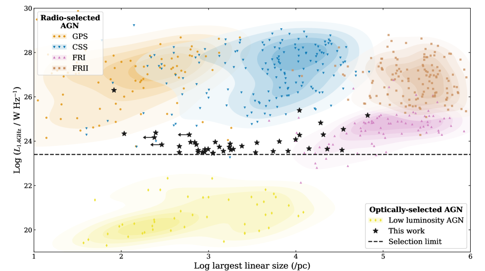
Figure 3: Radio luminosity versus largest linear size for the complete sample presented here (black stars) compared to the radio-selected AGN compiled by An & Baan (2012) (points and density contours of the appropriate shape / colour; see also Jarvis et al. 2019). Seyfert and LINER galaxies (‘low luminosity AGN’; Gallimore et al., 2006; Baldi et al., 2018) are shown for additional comparison. The black dashed line marks the radio luminosity selection criterion for our sample (log[$L_{\rm 1.4GHz}$ / W Hz^-1] $>23.4$). Our quasars share properties with the lowest luminosity compact radio galaxies (CSS / GPS) and the most compact, low luminosity, FRI radio galaxies. We suggest that at least some of the separation of the different populations are driven by selection effects (see Section 5.2).

4.2 Radio morphology

We classified the morphology observed in all three sets of radio images (LR, MR and HR; see Section 3.1) roughly following Baldi et al. (2018) and Kimball et al. (2011a). The classifications we have used are illustrated with examples from this work in Fig. 4 and are described below:

• Compact (C): if the source shows no visibly spatially-resolved features (i.e. has the appearance of a single two-dimensional Gaussian). We note that these sources may still be extended or elongated compared to the beam.

• Jet (J): if the source is composed of one contiguous feature, visibly spatially extended in one direction. We note that this definition is purely to describe the morphology, and may not be physically associated with an AGN-driven jet.

• Double (D): if the source shows two distinct peaks in the radio emission (i.e. the radio emission has the appearance of two two-dimensional Gaussian components).

• Triple (T): if the sources has three distinct radio peaks.

• Irregular (I): sources with spatially extended (irregular) radio morphologies that do not fit within the above categories.

• Undetected (U): if the source is not detected in the image.

Classifications were given by eye using the figures presented in Appendix Supporting Information by five of the authors. The final classification given to each source in each of the three images considered was taken to be the majority classification (in each case a minimum of three people agreed). These classifications are given in Table 2.

As expected, Table 2 shows that many more extended structures are seen in our highest resolution (HR) images compared to either our MR images or the LR images, with 36/42 classified as Compact in the LR images (i.e. the FIRST data) compared to just 18/42 in our HR images. On the other hand, it is important to note that some sources (e.g. J0907$+$4620 and J1016$+$0028; see Figs Supporting Information and Supporting Information) exhibit spatially diffuse extended features, visible at low resolutions, which are resolved out in our higher resolution images. Overall, we find that 28/42 (67 percent) of our sources show visibly extended features (i.e. any morphological classifications except for Compact) in at least one of the images. We discuss this fraction in the context of other samples in Section 5.3.1.

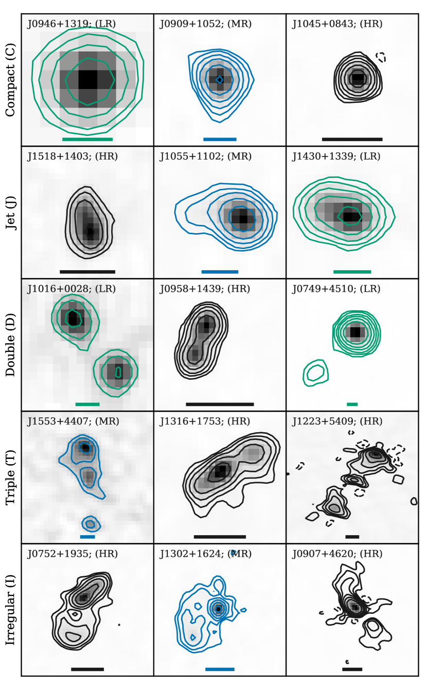
Figure 4: Examples of each of the morphological classifications used in this work as defined in Section 4.2. Each radio map is plotted both in grey-scale and with contours whose colour denotes the data displayed: green for FIRST (LR), blue for our MR data and black for our HR data. Contours are plotted at $\pm$[4, 8, 16, 32, 64, 128]$\sigma$, with negative contours marked by dashed lines. The size bar in each frame represents lengths of 11, 4 or 2 kpc for the LR, MR and HR data, respectively. These data are displayed in the context of the other radio data considered and the optical images for each source in Appendix Supporting Information.

The radio emission from star formation and AGN processes (jets, winds and coronal emission) can often be hard to distinguish, particularly for marginally resolved radio features, in galaxies undergoing mergers and in the absence of secondary spatially-resolved star-formation tracers (see e.g. Condon, 1992; Bondi et al., 2016; Alexandroff et al., 2016; Panessa et al., 2019; Chen et al., 2020; Smith et al., 2020). Therefore, we are conservative with our use of morphology to classify Radio-AGN. We only consider symmetric triple and double structures as they are very likely to be associated with a jet or loosely collimated wind (see e.g. Alexandroff et al., 2016; Baldi et al., 2018; Kimball et al., 2011a). Specifically, all five sources which were classified as triple (T; see Table 2) are classified as Radio-AGN and J0958$+$1439 and J1016$+$0028 (see Figs Supporting Information and Supporting Information) are classified as Radio-AGN because of their symmetric double structures (see also Jarvis et al., 2019).

4.3 Core spectral index

The identification of a flat spectrum radio core ($\alpha\gtrsim-$0.5; using $S_{\nu}\propto\nu^{\alpha}$) is considered a particularly strong criterion to positively identify an AGN with an active radio jet (see e.g. Orienti & Dallacasa, 2014; Panessa et al., 2019). Therefore, we measured the spectral index of the radio component best identified as the candidate ‘core’ from our HR images (4–8 GHz). For sources where there are multiple peaks in the image, we defined the candidate core to be either the brightest peak or the component with $\alpha>-$0.6, if one exists.

To measure the spectral indices we used the spectral index maps, and their respective error maps (see Section 3.1). We took the weighted average value of the $\alpha$ image within the 16$\sigma$ contour from the total intensity images, weighting by the squared inverse of the spectral index error map. We use the statistical error on the weighted average as the error on the final spectral index value. In a few cases, we were not able to use the 16$\sigma$ contour to reliably isolate the candidate core and so another $\sigma$ level was chosen (discussed on a case by case basis in Appendix Supporting Information). We note that using these different contour levels does not cause any of the measured values of $\alpha$ to change from a steep ($\alpha<-0.5$) to a flat ($\alpha$$\geq$$-0.5$) classification. For J1347+1217, since the available C-band VLA images did not contain spectral information, we instead took advantage of the fact that this source is unresolved at $\sim$0.3 arcsec scales and use the total spectral index from archival low resolution data (see Appendix Supporting Information).

The core spectral index for each source is listed in Table 2. Overall, we can state that at the flux and resolution limits of our data, we detect flat spectrum ($\alpha$$\geq$$-0.5$) cores in seven of our 42 sources. Unsurprisingly, all but one of the sources classified as ‘radio-loud’ following Xu et al. (1999) (Section 2.4) exhibit a flat spectral index and the exception is close to the flat/steep boundary (i.e. $\alpha=-0.6$ for J0907+4629). However, a further three of the sources with flat spectrum cores are classified as ‘radio-quiet’, demonstrating the limitations of traditional ‘radio-quiet’ versus ‘radio-loud’ definitions for identifying emission from jets in AGN (see also Section 5.1 and Padovani, 2016).

4.4 Brightness temperature

The bases of jets are expected to have high brightness temperatures (i.e. high levels of radio surface brightness) due to non-thermal processes from relativistic electrons (see e.g. Neff & de Bruyn, 1983; Preuss & Fosbury, 1983; Blundell & Beasley, 1998; Ulvestad et al., 2005; Alexandroff et al., 2012). We calculate brightness temperature ($T_{\mathrm{B}}$) in K for our sources following the standard equation:

$$T_{\textrm{B}}=\frac{1.8\times 10^{9}(1+z)S_{\nu}}{\nu^{2}\Theta_{\textrm{maj}}\Theta_{\textrm{min}}},$$ (3)

where $S_{\nu}$ is the peak flux density in mJy/beam, $\nu$ is the frequency in GHz, and $\Theta_{\textrm{maj}}$ and $\Theta_{\textrm{min}}$ are the source major and minor axis sizes respectively, deconvolved from the beam, in milliarcsec (following Ulvestad et al., 2005; Doi et al., 2013; Berton et al., 2018).

We calculated ${T}_{\textrm{B}}$ from our HR images using casa Gaussian fits (using the ‘imfit’ routine) to the central component to get the flux density, size and associated errors with each. For those with multiple central components in our HR image, either the brightest or the one with $\alpha>-0.6$ was used (as in Section 4.3). Four sources in our sample (J0749$+$4510, J1045$+$0843, J1100$+$0846 and J1300$+$0355) are reported as point sources using ‘imfit’ on the candidate core components. For these we used 1/2 of the beam size to derive lower limits on our $T_{\textrm{B}}$ calculation (following e.g. Doi et al., 2013). Two sources in the sample (J1356$+$1026 and J1553$+$4407) have errors on their minor axis size from ‘imfit’ which are larger than the value (giving sizes consistent with zero); for these sources we give a lower limit on the brightness temperature calculated using the ‘imfit’ major and minor sizes plus their associated errors.

The measured brightness temperatures for our sources span a broad range across $T_{\textrm{B}}=10^{2.5}$–$10^{8.5}$ K (ignoring lower limits) and are listed in Table 2. To classify sources as Radio-AGN based upon their brightness temperatures we used the Condon et al. (1991) theoretical upper limit due to compact starbursts. At the central wavelength of our C-band data this corresponds to values of $T_{\textrm{B}}>10^{4.6}$ K indicating a Radio-AGN.

We note that due to the relatively large spatial resolution of our observations ($\sim$0.3 arcsec) compared to the very long baseline interferometry (VLBI) observations that are typically used for investigating brightness temperatures (e.g. Falcke et al., 2000; Nagar et al., 2005), even our deconvolved sizes could overestimate the true size of the radio cores, artificially decreasing the observed brightness temperature. Nonetheless, even given these limitations, seven of our sample have brightness temperatures indicative of AGN activity (see Table 2).

4.5 Radio excess

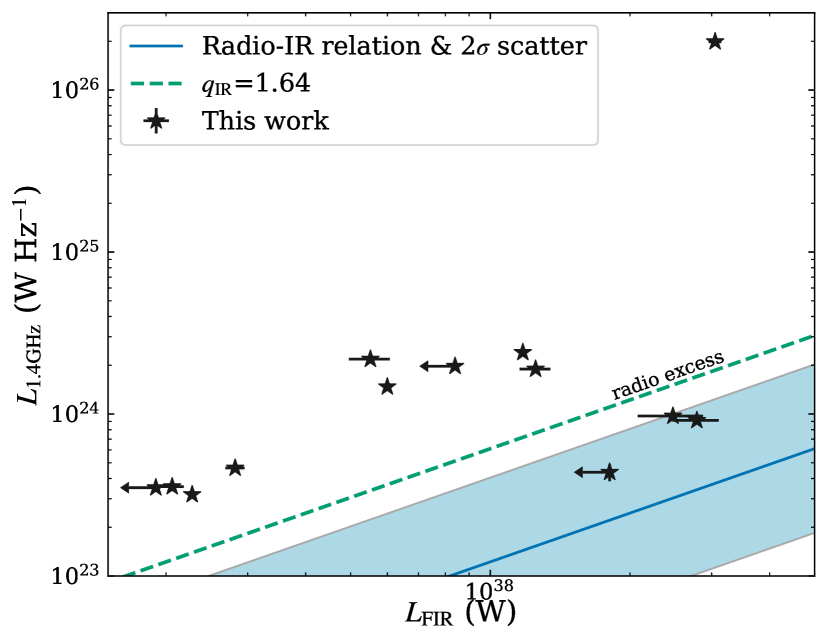
Figure 5: The observed radio luminosity from NVSS compared to the far-infrared (42.5–122.5 $\mu$m) luminosity calculated from the observed IRAS / PACS photometry for the 13 sources with the required data (black stars; the errors on the 1.4 GHz luminosity are typically smaller than the point size). The green dashed line marks $q_{\textrm{IR}}=1.64$ and is the threshold where there is confirmed excess radio emission over that expected from star formation (see Section 4.5), with all but three of our sources falling in the radio excess region. The blue solid line and shaded region represent the radio–IR correlation for normal star forming galaxies and the 2$\sigma$ scatter on the relation from Bell (2003).

Both star formation and AGN related processes are capable of producing 1.4 GHz radio luminosities comparable to those observed in our sample (see e.g. Condon, 1992). However, sources with significant radio emission above the well-established radio–IR correlation of normal star-forming galaxies (Helou et al. 1985; Bell 2003) can be identified as Radio-AGN (e.g. Del Moro et al., 2013; Padovani, 2016; Smith et al., 2020).

We calculated the far infrared flux ($S_{\textrm{FIR}}$; 42.5–122.5 $\mu$m) for each of our sources following Helou et al. (1985) (see also Marvil et al., 2015):

$$S_{\textrm{FIR}}=1.26\times 10^{-14}(2.58S_{60\mu\textrm{m}}+S_{100\mu\textrm{m}})\textrm{W m}^{-2},$$ (4)

where $S_{60\mu\textrm{m}}$ and $S_{100\mu\textrm{m}}$ are the rest frame 60 and 100 $\mu$m flux densities in Jy. We then calculated the offset of a source relative to the radio–IR correlation, $q_{\textrm{IR}}$, following:

$$q_{\textrm{IR}}=\log\left(\frac{S_{\textrm{FIR}}}{3.75\times 10^{12}\textrm{W m}^{-2}}\right)-\log\left(\frac{S_{\textrm{1.4GHz}}}{\textrm{W m}^{-2}\textrm{Hz}^{-1}}\right),$$ (5)

where $S_{\textrm{1.4GHz}}$ is the K-corrected 1.4GHz radio flux density. We calculated the error on $q_{\textrm{IR}}$ from the reported catalogue errors on the flux density measurements.

We obtained the necessary rest-frame flux density measurements by linearly interpolating the Infrared Astronomical Satellite (IRAS; Neugebauer et al., 1984) 60 and 100 $\mu$m flux densities or, if available, the ESA Herschel Space Observatory PACS point source catalogue’s 70 and 100 $\mu$m flux densities and associated errors (Pilbratt et al., 2010; Poglitsch et al., 2010). We used IRAS measurements from the faint source catalogue (FSC; Moshir et al., 1992). Following Wang et al. (2014), we followed a log likelihood method of matching IRAS to the closest Wide-field Infrared Survey Explorer (WISE) all-sky survey (Wright et al., 2010) source to the SDSS position ($<$ 2 arcsec) to account for the large and asymmetric IRAS beam. For sources detected in one band but not the other, we assume an upper limit on the FIR flux. We also note that upper limits from IRAS for sources not detected at either 60 or 100 $\mu$m are not sufficiently constraining to reliably identify radio excess AGN (with the exception of the traditional ‘radio-loud’ AGN); therefore, we only perform these analyses on the 13 sources with at least one detection across the relevant IRAS or PACS bands.

We show the position of our sources with measured IR values compared to the relation for star-forming galaxies in Fig. 5. It can be seen that the majority of our targets lie above the relationship. Following other works we use $q_{\textrm{IR}}<1.64$ to define a significant offset from the radio–IR correlation and refer to these as ‘radio excess’ (Helou et al. 1985; see also Marvil et al. 2015). Of the 13 sources, we find that ten are defined as radio excess, one has a non-constraining limit (J1355$+$2046 with $q_{\textrm{IR}}<2.04$) and two sources have $q_{\textrm{IR}}$ values that fall within the region occupied by star-forming galaxies. However, we cannot rule out that the two sources which appear to lie on the relation have an AGN contribution to their FIR emission and hence should intrinsically lie above the relation (see e.g. Morić et al., 2010; Bonzini et al., 2013; Zakamska et al., 2016a; Wong et al., 2016). Indeed, one of these targets (J1108$+$0659) is identified as an AGN based on literature information (see Appendix Supporting Information), and another (J1509$+$1757) is borderline radio-loud by the criterion of Ivezić et al. (2002) (with $R=1.0$; see Table 2 and Section 2.4).

Overall, we conclude that 10/13 (77 percent) of our sample for which we have the necessary constraints on the FIR emission are classified as radio excess and, consequently, at least 10/42 (24 percent) across the full sample have excess radio emission above what can be explained by star formation.

4.6 Final identification of radio emission from AGN

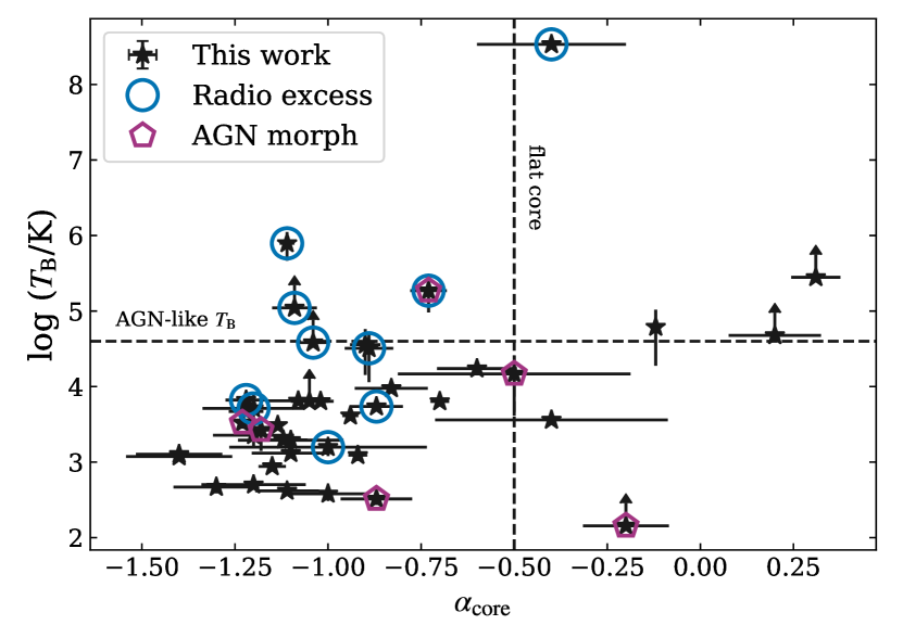
Figure 6: This figure illustrates the four commonly used criteria used to separate targets with a Radio-AGN from those where the radio emission could be dominated by star formation which we combine in this work (see Section 4). The logarithm of the brightness temperature is plotted against the spectral index of the radio component identified as the core (black stars). The vertical dashed line indicates a flat spectrum core (i.e. $\alpha_{\textrm{core}}\geq-0.5$) and the horizontal dashed line indicates high brightness temperatures (i.e. log $T_{\textrm{B}}$ $\geq$ 4.6), each of which imply an AGN origin of the radio emission (see Section 4.3 and 4.4). Sources that were identified as radio excess (see Section 4.5 and Fig. 5) and those with radio morphology strongly suggestive of AGN radio emission (see Section 4.2) are additionally plotted with blue circles and/or magenta pentagons respectively, on top of the black stars used for the entire sample. Sources satisfying at least one of these criteria are considered Radio-AGN in this work with many satisfying multiple criteria. Due to a non detection we were unable to calculate a core spectral index or brightness temperature for J1016$+$0028; however, it is classified as a Radio-AGN based on its morphology.

By constraining the dominant physical mechanisms contributing to the radio emission in our sample we gain a deeper understanding of the energy balance in the galaxy and the possible drivers of outflows (e.g. Nims et al., 2015; Harrison et al., 2018). Here we identify sources where we attribute the radio emission to an AGN, i.e. ‘Radio-AGN’, by combining the four criteria described in the previous sub-sections. As previously discussed, these are all well established methods for identifying Radio-AGN, and we apply them here to our unique sample (see Section 2.3). We put equal weight on all methods and consider any source which is deemed to be AGN-like in at least one to be a Radio-AGN. Our final classification process is presented in Fig. 6, and is summarised as follows:

1. Seven of our sources are Radio-AGN based on the identification of a flat spectrum core ($\alpha\geq-0.5$; see Section 4.3).

2. 10 of our 13 sources, for which we have meaningful constraints, have measured radio excess values indicative of AGN with $q_{\textrm{IR}}<1.64$ (see Section 4.5). Only one of these is classified as a Radio-AGN based on having a flat spectrum core, bringing our total number of Radio-AGN in this sample up to 16.

3. Seven sources have brightness temperatures indicating that their core radio emission is dominated by AGN related processes (Section 4.4). All seven of these have been identified as Radio-AGN based on either their spectral index and/or their $q_{\textrm{IR}}$ values.

4. Seven sources are classified as Radio-AGN based upon their morphology (Section 4.2), adding four sources which were not classified as Radio-AGN based on the criteria described above. This brings the total number of Radio-AGN up to 20 and these are labelled with a ‘yes’ in the final column of Table 2.

The limitations of each of the methods we applied are discussed in the relevant sub-sections. In each case we conclude that our approach is conservative and the true number of Radio-AGN is likely to be higher than that finally quoted here. In particular, more extensive far-infrared data is likely to increase the number of sources identified as ‘radio excess’ and higher spatial resolution and/or higher frequency radio data, would likely increase the number of identified flat spectrum or high brightness temperature sources (see e.g. Smith et al., 2020). Indeed, four of the sources in our sample which are not classified as Radio-AGN by the method described above, have been previously identified as hosting compact jets in the literature by using higher spatial resolution radio imaging, classical radio-loudness and/or a more detailed treatment of the far-infrared data. These are J0907$+$4620, J1010$+$1413, J1108$+$0659 and J1715$+$6008 and are labelled as ‘yes^∗’ in the final column of Table 2 (see details in Appendix Supporting Information, Supporting Information, Supporting Information and Supporting Information). In line with our overall goal of identifying as many Radio-AGN in our sample as possible, we include these four sources as Radio-AGN.

Overall, we conservatively conclude that at least 24/42 (57 percent) of the sample can be classified as Radio-AGN (20/42 if only the data presented in this paper are considered). For the rest of the sample, the origin of the radio emission is unclear, with star formation or the AGN both as viable possibilities.

5 Discussion

Using VLA observations of 42 luminous quasars (Fig. 1) we have found that they have radio sizes ranging from LLS $=$ 0.08–66.5 kpc (with three unresolved sources; see Section 4.1 and Fig. 3). For 67 percent of the sample we identified radio structures on 1–60 kpc scales (Section 4.2). Overall, by combining four different well-known diagnostics we have found that at least 57 percent of our sample can be classified as ‘Radio-AGN’ (Section 4.6). Here we discuss these results in the context of commonly used selection criteria of selecting ‘radio-loud’ AGN (Section 5.1) and compare the radio properties of this sample to typical ‘radio-loud’ samples (Section 5.2). Finally, we explore the relationship between the ionised gas and radio properties of our sources and discuss what this might mean for understanding the feedback processes in quasar host galaxies (Section 5.3).

5.1 Comparison to diagnostics to identify radio-loud AGN

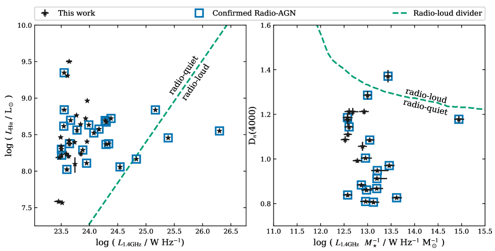
Figure 7: Our targets plotted in two diagnostic plots that are designed to separate radio-loud and radio-quiet AGN (black stars; see Section 5.1). Left: H$\alpha$ versus 1.4 GHz radio luminosity. Right: D_n4000 versus the ratio of the 1.4 GHz radio luminosity to the stellar mass for the Type 2 AGN in our sample. We note that the error-bars in both panels are often smaller than the point sizes. Our targets that are confirmed as Radio-AGN from our analyses (Section 4.6) are further marked with blue squares in addition to the black stars used for the overall sample. All but four of our targets fall into the radio-quiet, candidate star-formation dominated, area of the figures, confirming that these diagnostics are not effective for finding low power Radio-AGN associated with powerful quasars.

As already discussed in Section 2.4, the ‘radio-loud’ division of Xu et al. (1999) only identifies five sources in our sample (see Fig. 1) and a further four of the Type 1 targets are moderately ‘radio-loud’ based on the $R$ value (Ivezić et al. 2002). Another widely adopted method for identifying ‘radio-loud’ AGN are the criteria of Best & Heckman (2012) (see also Sabater et al., 2019). Specifically, they used three diagnostics: one compares the observed radio emission to H$\alpha$ luminosity, because both of these are star-formation tracers for star-forming galaxies. Another diagnostic compares the strength of spectral break at 4000Å (D_n4000; a tracer of mean stellar age), which correlates with the ratio of radio luminosity to stellar mass for star forming galaxies. Finally, they used emission-line ratio diagnostics as part of their selection criteria; however, we do not discuss this here because our sample was selected as AGN based on their optical emission line properties (Mullaney et al., 2013).

We compare our classification from Section 4.6 to what we would have found using the Best & Heckman (2012) diagnostics in Fig. 7. For our targets we use the H$\alpha$ emission-line fluxes from Mullaney et al. (2013) and we take both D_n4000 and stellar mass ($M_{\star}$) from MPA-JHU SDSS DR8 measurements converted from a Kroupa to Chabrier IMF (Madau & Dickinson, 2014). We note that these stellar masses are calculated using optical SED fitting without considering AGN emission, and so are particularly unreliable for the Type 1 AGN in this sample (where the optical emission is expected to be dominated by the AGN). As such, the Type 1 sources are excluded from the diagnostic using stellar masses. However, we note that if we use the AGN-corrected stellar masses for the nine Type 2 AGN presented in Jarvis et al. (2019), the classifications do not change, and we therefore conclude that these mass measurements are suitable for the Type 2 sources.

In Fig. 7 it can be seen that only one source (J0907$+$4620) based on the D_n4000 diagnostic and only three sources (J1223$+$5409, J1347$+$1217 and J1701$+$2226) based on the H$\alpha$ diagnostic are classified as radio-loud. These four are a subset of the five classical ‘radio-loud’ sources identified by the Xu et al. (1999) division (see Table 2 and Fig. 1). This result is not surprising since these criteria are not designed to be complete but, instead, to cleanly select sources where the radio emission is definitely dominated by the AGN (Best & Heckman, 2012; Sabater et al., 2019). In particular, the H$\alpha$ diagnostic is based on the assumption that for the galaxy population of interest, H$\alpha$ is a reliable star-formation diagnostic. It is therefore expected that this criterion will not be effective if applied to the most radiatively luminous AGN that are selected with emission lines, such as our sample, since the H$\alpha$ emission will have a strong, potentially dominant, contribution from the AGN (e.g. Kewley et al. 2001; Scholtz et al. 2020). This current work confirms that applying a combination of Radio-AGN selection methods, including the use of high-resolution radio imaging (Section 4), is important to obtain a more complete identification of Radio-AGN for the type of quasars studied here (i.e. moderate radio luminosity, [O iii] luminous AGN).

5.2 Comparison to traditional radio-loud AGN samples

Combining our measured sizes with the total radio luminosities from NVSS ($L_{\textrm{1.4GHz}}$; see Table 1) we compare the radio properties of our sample to those of traditional radio-loud AGN from An & Baan (2012) in Fig. 3. As can be seen in this figure, the sizes we measure for our sample ($\sim$0.1–10 kpc) are broadly consistent with those found in samples of compact ‘radio-loud’ AGN with jets (in this case represented primarily by GHz-Peaked Spectrum – GPS – and Compact Steep Spectrum – CSS – sources). Most of our sources would be excluded from such samples due to their lower radio luminosities and not being classified as radio-loud AGN by traditional methods (Section 5.1).

The largest sources in our sample (i.e. those with radio sizes $\gtrsim$10 kpc) overlap with the tail of the smallest, dimmest Fanaroff-Riley class I radio galaxies (FRI; Fanaroff & Riley, 1974, see Fig. 3). The smallest FRI sources in the An & Baan (2012) sample are from Fanti et al. (1987) which has spatial resolutions down to $\sim$1 arcsec (in comparison, our smallest resolution is $\sim$0.3 arcsec). This, combined with differences in sample selection and how the radio sizes are measured between this work and Fanti et al. (1987), implies that the smaller sizes in our sample compared to typical FRI sources could be mostly driven by a resolution / measurement effect.

Overall, our observations are consistent with other radio studies of quasars, using both low and high frequency data, which show a wide range of radio properties (e.g. we see no clear bimodality in the size and luminosity distributions; Mahony et al., 2012; Gürkan et al., 2019). Our sources have an interesting moderate radio luminosity range, with median $L_{\rm 1.4GHz}\approx 10^{23.8}$, where AGN may be expected to start to dominate the radio emission, but where they are excluded from traditional ‘radio-loud’ samples (Kimball et al., 2011b; White et al., 2015; Kellermann et al., 2016; Zakamska et al., 2016a; White et al., 2017). Indeed, the majority of our targets do not fit neatly within the traditional FRI and FRII radio classifications. Although deeper data may help determine the relative contributions of jets, lobes and hot spots, our results and recent results in the literature demonstrate that high spatial resolution images of low power Radio-AGN can reveal much more complexity in radio morphologies than that seen in the traditional ‘FRI’ and ‘FRII’ radio galaxies (e.g. Mingo et al., 2019). Many of our sources have featureless radio morphology (i.e. our ‘C’ classification), particularly in the lower resolution images and as such could be classified as ‘FR0’ galaxies according to some classification schemes (e.g. Baldi et al., 2015). However, higher spatial resolution data may reveal more complex morphologies on smaller scales (see discussion in Hardcastle & Croston, 2020).

We also note that several of our sources show radio morphologies similar to those typically seen in Seyfert galaxies. Specifically, Seyferts often show ‘C shaped’, ‘S shaped’ or ‘figure-8 shaped’ radio structures on 1-10 kpc scales (see e.g. Duric & Seaquist, 1988; Wehrle & Morris, 1988; Kharb et al., 2006, 2016). Similar structures are seen in this sample in e.g. J0752$+$1935, J0907$+$4620, J1000$+$1242, 1302$+$1624 and J1430+1339 (see Figs Supporting Information, Supporting Information, Supporting Information, Supporting Information and Supporting Information). This suggests that there is a continuity in the radio properties of quasars and Seyferts.

5.3 The ionised gas – radio connection

Here, we compare the radio sizes of our sample to the [O iii] luminosities and line widths. We use this to explore the connection between the ionised gas and the radio emission in our sample and compare this to other AGN samples in the literature.

5.3.1 Prevalence of radio structures with high [O iii] luminosity

In Section 4.2 we found that 67 percent of our sample show spatially extended features on kiloparsec scales. This is a marginally higher fraction than has been found in previous spatially resolved radio studies of ‘radio-quiet’ quasars with similar radio luminosities (specifically Kukula et al. 1998 which found extended features in $\sim$50 percent of their sample and 44 percent in Pierce et al. 2020). Compared to these works the main difference of this study is the selection of sources with $L_{\rm[O~{}III]}$$>10^{42.1}$ erg s^-1. Specifically, the selection criteria in Pierce et al. (2020) are almost identical to those in this work with the exception that their sample all have $L_{\rm[O~{}III]}$$<$10⁴² erg s^-1. Importantly, their radio observations are comparable to ours (i.e. VLA L- and C-band A-array configuration data with similar observation times and rms noise levels).

For compact powerful radio galaxies (e.g. CSS / GPS sources), there is a generally accepted link between [O iii] luminosity and radio size (see review in O’Dea & Saikia 2020). This has traditionally been reported as a trend for larger radio sizes to be associated with higher [O iii] luminosities (see e.g. O’Dea 1998; Labiano 2008). Although this trend is weak (see Kunert-Bajraszewska & Labiano, 2010), there is a distinct lack of the most compact radio sources (i.e. $\lesssim$0.1 kpc) at the most extreme [O iii] luminosities (i.e. $L_{\textrm{ [O~{}{\sc iii}]}}\gtrsim 10^{42}$ erg s^-1). To investigate this further, in Fig. 8 we show the radio sizes and [O iii] luminosities from our pre-dominantly radio-quiet sources and those of the radio-loud sources from Liao & Gu (2020), who also used SDSS spectroscopy to make their [O iii] emission-line measurements.

As can be seen in Fig. 8, our data suggest that the trend between radio size and [O iii] luminosity observed in radio-loud populations also holds for radio-quiet AGN (see also Leipski et al. 2006). The [O iii] bright sources in the Liao & Gu (2020) radio-loud sample (i.e. those with $L_{\rm[O~{}III]}$$>$10⁴² erg s^-1) all have sizes $\geq$0.75 kpc, similar to the smallest sizes measured in this work (see Fig. 8). This provides a possible explanation for why we find a larger fraction of spatially extended sources than the radio-quiet, lower [O iii] luminosity sample of Pierce et al. (2020). This could also explain why we found a higher fraction of spatially extended sources in our pilot study of Jarvis et al. (2019) ($\sim$80–90 percent), since the subset of targets in that work all fall at the higher [O iii] luminosity end of the current sample (median $L_{\rm[O~{}III]}$ = 4.7$\times$10⁴² erg s^-1, compared to 2.1$\times$10⁴² erg s^-1 for the complete sample presented here; see Fig. 1).

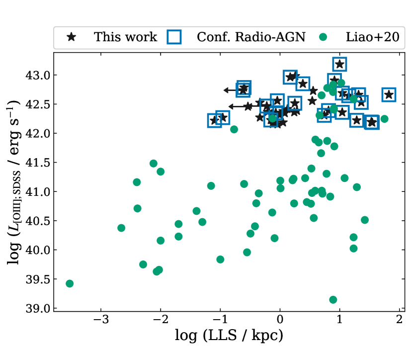
Figure 8: [O iii] luminosity (from SDSS single Gaussian fits) versus largest linear size (LLS) of the radio emission. We plot the sample presented here (black stars) and the SDSS matched radio-loud sample of Liao & Gu (2020) (green circles; see Section 5.3.1). The sources in our sample which we were able to confirm as Radio-AGN (see Section 4.6) are additionally marked with blue squares on top of the black stars used for the entire sample. High $L_{\rm[O~{}III]}$ AGN seem to be preferentially associated with larger radio sources, where less [O iii] luminous AGN can be associated with a wide range of radio sizes (see Section 5.3.1).

5.3.2 Radio sizes related to ionised gas kinematics

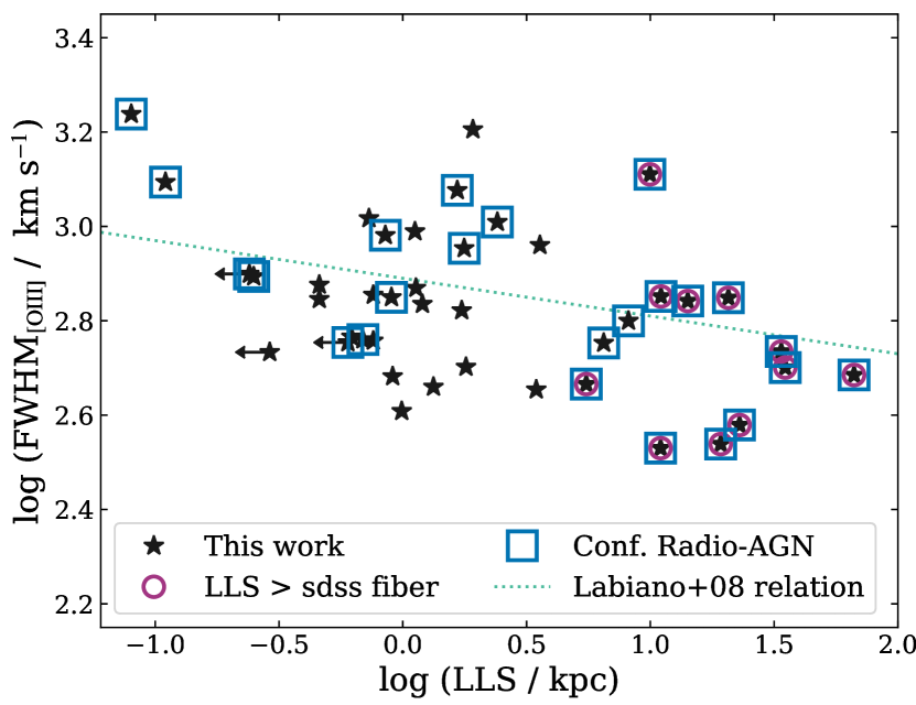
Figure 9: Flux-weighted FWHM of the [O iii] line from the two Gaussian fits of Mullaney et al. (2013) (see Table 1) compared to the largest linear size (LLS) calculated in this work (see Table 2; black stars). The sources for which we have a confirmed Radio-AGN classification (see Section 4.6) are further marked with blue squares on top of the black stars used for the entire sample. Magenta circles on top of the black stars additionally mark those whose LLS is larger than the SDSS fibre. For comparison, we include the linear fit to archival compact radio-loud AGN from Labiano (2008) (green dotted line). Larger radio sources are preferentially associated with galaxies with less extreme [O iii] kinematics than more compact sources.

An association between the most extreme ionised outflows and the most compact radio galaxies has previously been reported for ‘radio-loud’ populations (see e.g. Gelderman & Whittle, 1994; Best et al., 2000; Holt et al., 2008; Kim et al., 2013). Molyneux et al. (2019) provided indications of such a link in radio-quiet AGN. Here we use our measurements, that use $\sim$20 times better spatial resolution radio images than Molyneux et al. (2019), to test this result on our pre-dominantly radio-quiet quasar sample.

In Fig. 9 we compare the radio sizes of the sources from our sample (see Table 2) to the flux-weighted FWHM from the Mullaney et al. (2013) two Gaussian fits to the [O iii] line profile (Table 1). We find evidence for a negative correlation between the FWHM and the radio size. Although there is a large scatter, the existence of this correlation is supported by a Spearman rank correlation coefficient of $-$0.42 and p-value for a null hypothesis of uncorrelated data of 0.008 (excluding upper limits). We note that some of the scatter we find in this relation could be the result of different levels of projection effects affecting the observed radio sizes. The results presented in Fig. 9 are in qualitative agreement with the results of Molyneux et al. (2019).

A thorough, quantitative comparison between the trend demonstrated in this work and that found in the literature is difficult due to the relatively small samples and/or inhomogeneous datasets involved. Nonetheless, Holt et al. (2008) find that extended radio-loud AGN (radio sizes greater than 30 kpc) typically have [O iii] FWHM values around 200-300 km s^-1, while compact radio sources (radio sizes less than 30 kpc) have typical [O iii] FWHM values of around 1000 km s^-1. These values are consistent with the results presented here. A more direct comparison can also be made with the work of Labiano (2008), whose radio-loud CSS / GPS sample spans a similar range of [O iii] luminosities and radio sizes to the sample presented here (approximately $10^{41}<$ $L_{\rm[O~{}III]}<10^{44}$ erg s^-1 and 0.1 $<$ LLS $<$ 10 kpc ) but with significantly higher radio luminosities ($L_{\textrm{1.4GHz}}\gtrsim 10^{25}$ W Hz^-1). We show the relationship from Labiano (2008) in Fig. 9, which is qualitatively similar to the trend seen for our sample. Nonetheless, the relation between the width of the [O iii] emission line and the radio size found in both samples is weak and larger, more homogeneous samples are required for a robust quantification of the slope and scatter of this relationship.

Overall, we conclude that the connection between ionised gas kinematics and radio emission, seen in powerful ‘radio-loud’ AGN is also seen in the lower radio luminosity systems of our sample.

5.3.3 Implications for how quasars interact with the ISM

Across our sample the high fraction of extended radio sources (Fig. 3) and the observed connection between both the [O iii] luminosity and ionised gas kinematics with the size of the radio emission (Fig. 8 and Fig. 9) could be explained by either jets or quasar-driven winds interacting with the ISM. Both mechanisms would be able to ionise larger volumes of gas as they expand / age (Bicknell et al., 1997; Moy & Rocca-Volmerange, 2002; Vink et al., 2006; Jiang et al., 2010; Nims et al., 2015; Mukherjee et al., 2018), resulting in more extreme [O iii] luminosities preferentially associated with extended radio emission. Additionally, as the jet / wind expands, interactions with the ISM could cause deceleration, which would result in the observed lower velocities (traced by the FWHM of the [O iii] emission) for larger radio sources (see e.g. Wagner et al., 2012; Labiano, 2008; Dugan et al., 2017; Bicknell et al., 2018; Mukherjee et al., 2018, 2020). Furthermore, both winds and low power jets will preferentially take the path of least resistance through a clumpy medium resulting in less interaction, and hence a smaller velocity dispersion, with the gas at larger scales where the gas density drops (Mukherjee et al., 2018; Costa et al., 2014; Costa et al., 2018).

Therefore, the observations we have made could provide evidence for a strong interaction between either radio jets or quasar-driven winds and the interstellar medium. Indeed, direct evidence for this is shown by combining radio imaging with integral field spectroscopy for nine of the targets in Jarvis et al. (2019). Furthermore, it is interesting to note that over half of our sources (24) have steep core spectral indices with $\alpha\leq-1$ (see Table 2), steeper than the typically observed value of around $-0.7$. Radio emission originating from shocked quasar winds has been predicted to have spectral indices closer to $-$1 (Nims et al., 2015). Strong radiative losses due to interactions between jets and the ISM could also result in a steep spectral index (see e.g. Congiu et al., 2017). Spatially-resolved studies of both the radio properties and the multi-phase gas kinematics, will greatly increase our understanding of how typical, radio-quiet AGN and quasars interact with their host galaxies (e.g. Venturi et al., 2020).

6 Conclusions

We have presented the first results on our sample of 42 $z<0.2$, [O iii] luminous AGN ($L_{\rm[O~{}III]}>10^{42.1}$ ergs s^-1) from our Quasar Feedback Survey. The targets represent the 30 percent of the parent AGN population, in this redshift and [O iii] luminosity range, which have radio luminosities of $L_{\rm 1.4GHz}>10^{23.4}$ W Hz^-1 (see Section 2.2). Overall they have moderate radio luminosities (median $L_{\rm 1.4GHz}=5.9\times 10^{23}$ W Hz^-1). Here we have presented spatially resolved radio images at 1.5 GHz and 6 GHz with around 1 and 0.3 arcsec resolution for the full sample (e.g. Fig. 2). We have confirmed the importance of using high resolution radio images, i.e. beyond that typically available for all-sky radio surveys, to identify ‘Radio-AGN’ (Section 4.2). By combining our new radio images with archival information, we investigated the source of the radio emission and the relationship between the radio emission and the [O iii] emission-line properties.

Our main conclusions are as follows:

1. 28 out of the 42 targets (i.e. 67 percent) show morphologically distinct spatially extended radio features on scales of $\gtrsim$0.3 arcsec with a diverse range of morphologies (see Fig. 4). We measured the radio sizes of our sources to be 0.08 $<$ LLS $<$ 66.5 kpc. These sizes are comparable to those observed for compact radio galaxy samples (e.g. CSS / GPS sources) that typically have radio luminosities that are at least 2 orders of magnitude higher than our sample (see Section 5.2 and Fig. 3).

2. Only 4–9 of the sample are radio-loud by traditional criteria (see Section 2.4, Section 5.1, Figs 1 and 7). However, at least 24/42 (57 percent) have a strong indication of radio emission associated with an AGN. This is determined by combining a series of well-known Radio-AGN selection techniques that use measurements of: the radio–infrared excess parameter; the core spectral index; the brightness temperatures and radio morphologies (see Section 4.6, Fig. 5 and Fig. 6). We are unable to draw definitive conclusions on the origin of the radio emission in the remainder of the targets without further data.

3. We confirmed that there is a link between both the luminosity and the width of the [O iii] emission line and the radio size in ‘radio-quiet’ quasars that is similar to that which has previously been observed for ‘radio-loud’ AGN. Specifically, [O iii] luminous sources are more likely to have extended radio emission and larger radio sources tend to have narrower [O iii] lines. This suggests that the radio and ionised gas properties in radio-quiet quasars are closely connected (see Section 5.3, Fig. 8 and Fig. 9).

This work is the first to examine the properties of the full Quasar Feedback Survey sample (Fig. 1). We find that the AGN contribute significantly to the radio emission even though the sample are bolometrically luminous quasars and the majority of the targets are classically ‘radio-quiet’. This result suggests that care should be taken when considering the division of feedback into ‘radio’ and ‘quasar’ modes.

Some of the ongoing work we are pursuing in the Quasar Feedback survey includes exploring the radio SEDs and obtaining higher spatial resolution radio observations to distinguish the forms of radio emission in this sample (e.g. jets verses shocks from quasar-driven winds). We will also present spatially-resolved ionised gas and molecular gas measurements for subsets of the sample, to explore in more detail the multi-phase outflows and ISM properties (e.g. Girdhar et al. in prep), building on the preliminary work presented in Jarvis et al. (2019, 2020) on the pilot sample. As such, this paper represents a first step towards a detailed understanding of the mechanisms and impact of AGN feedback in this unique sample of quasars.

Data Availability

The data underlying this article were accessed from the NRAO Science Data Archive (https://archive.nrao.edu/archive/advquery.jsp) using the proposal ids: 13B-127 and 18A-300. The radio images produced for this work are available from Newcastle University’s data repository (https://data.ncl.ac.uk/projects/Quasar_Feedback_Survey/92264) and can also be accessed through our website: (https://blogs.ncl.ac.uk/quasarfeedbacksurvey/data/).

Supporting Information

Supplementary data are presented in a companion PDF.

Appendix A. Observations and Images.

Table A1. The key properties of the VLA observations and images used in this work.

Appendix B. Images and notes on individual objects.

Figures B1–B41. As Fig. 2 but for remainder of sample.

References

- Ahumada et al. (2020) Ahumada R., et al., 2020, ApJS, 249, 3
- Alexander & Hickox (2012) Alexander D. M., Hickox R. C., 2012, New Astron. Rev., 56, 93
- Alexandroff et al. (2012) Alexandroff R., et al., 2012, MNRAS, 423, 1325
- Alexandroff et al. (2016) Alexandroff R. M., Zakamska N. L., van Velzen S., Greene J. E., Strauss M. A., 2016, MNRAS, 463, 3056
- An & Baan (2012) An T., Baan W. A., 2012, ApJ, 760, 77
- Baldi et al. (2015) Baldi R. D., Capetti A., Giovannini G., 2015, A&A, 576, A38
- Baldi et al. (2018) Baldi R. D., et al., 2018, MNRAS, 476, 3478
- Balmaverde et al. (2020) Balmaverde B., et al., 2020, arXiv e-prints, p. arXiv:2010.11195
- Baron et al. (2018) Baron D., et al., 2018, MNRAS, 480, 3993
- Becker et al. (1995) Becker R. H., White R. L., Helfand D. J., 1995, ApJ, 450, 559
- Begelman & McKee (1983) Begelman M. C., McKee C. F., 1983, ApJ, 271, 89
- Behar et al. (2018) Behar E., Vogel S., Baldi R. D., Smith K. L., Mushotzky R. F., 2018, MNRAS, 478, 399
- Bell (2003) Bell E. F., 2003, ApJ, 586, 794
- Berton et al. (2018) Berton M., et al., 2018, A&A, 614, A87
- Best & Heckman (2012) Best P. N., Heckman T. M., 2012, MNRAS, 421, 1569
- Best et al. (2000) Best P. N., Röttgering H. J. A., Longair M. S., 2000, MNRAS, 311, 23
- Bicknell et al. (1997) Bicknell G. V., Dopita M. A., O’Dea C. P. O., 1997, ApJ, 485, 112
- Bicknell et al. (2018) Bicknell G. V., Mukherjee D., Wagner A. e. Y., Sutherland R. S., Nesvadba N. P. H., 2018, MNRAS, 475, 3493
- Bischetti et al. (2020) Bischetti M., et al., 2020, arXiv e-prints, p. arXiv:2009.01112
- Blandford & Payne (1982) Blandford R. D., Payne D. G., 1982, MNRAS, 199, 883
- Bluck et al. (2020) Bluck A. F. L., et al., 2020, arXiv e-prints, p. arXiv:2009.05341
- Blundell & Beasley (1998) Blundell K. M., Beasley A. J., 1998, MNRAS, 299, 165
- Bondi et al. (2016) Bondi M., Pérez-Torres M. A., Piconcelli E., Fu H., 2016, A&A, 588, A102
- Bonzini et al. (2013) Bonzini M., Padovani P., Mainieri V., Kellermann K. I., Miller N., Rosati P., Tozzi P., Vattakunnel S., 2013, MNRAS, 436, 3759
- Bradley et al. (2019) Bradley L., et al., 2019, astropy/photutils: v0.6. Zenodo, doi:10.5281/zenodo.2533376
- Briggs (1995) Briggs D., 1995, PhD thesis, The New Mexico Institute of Mining and Technology, Socorro, New Mexico, -
- Brownson et al. (2020) Brownson S., Belfiore F., Maiolino R., Lin L., Carniani S., 2020, MNRAS, 498, L66
- Brusa et al. (2015) Brusa M., et al., 2015, MNRAS, 446, 2394
- Carniani et al. (2015) Carniani S., et al., 2015, A&A, 580, A102
- Chabrier (2003) Chabrier G., 2003, PASP, 115, 763
- Chartas et al. (2020) Chartas G., et al., 2020, MNRAS, 496, 598
- Chen et al. (2020) Chen S., et al., 2020, arXiv e-prints, p. arXiv:2006.01700
- Circosta et al. (2018) Circosta C., et al., 2018, A&A, 620, A82
- Condon (1992) Condon J. J., 1992, ARA&A, 30, 575
- Condon et al. (1991) Condon J. J., Huang Z. P., Yin Q. F., Thuan T. X., 1991, ApJ, 378, 65
- Condon et al. (1998) Condon J. J., Cotton W. D., Greisen E. W., Yin Q. F., Perley R. A., Taylor G. B., Broderick J. J., 1998, AJ, 115, 1693
- Condon et al. (2013) Condon J. J., Kellermann K. I., Kimball A. E., Ivezić Ž., Perley R. A., 2013, ApJ, 768, 37
- Congiu et al. (2017) Congiu E., et al., 2017, A&A, 603, A32
- Costa et al. (2014) Costa T., Sijacki D., Haehnelt M. G., 2014, MNRAS, 444, 2355
- Costa et al. (2018) Costa T., Rosdahl J., Sijacki D., Haehnelt M. G., 2018, MNRAS, 479, 2079
- Cresci & Maiolino (2018) Cresci G., Maiolino R., 2018, Nature Astronomy, 2, 179
- Davies et al. (2020a) Davies R., et al., 2020a, MNRAS, 498, 4150
- Davies et al. (2020b) Davies R. L., et al., 2020b, ApJ, 894, 28
- Del Moro et al. (2013) Del Moro A., et al., 2013, A&A, 549, A59
- Dey et al. (2019) Dey A., et al., 2019, AJ, 157, 168
- Doi et al. (2013) Doi A., Asada K., Fujisawa K., Nagai H., Hagiwara Y., Wajima K., Inoue M., 2013, ApJ, 765, 69
- Dugan et al. (2017) Dugan Z., Gaibler V., Silk J., 2017, ApJ, 844, 37
- Duric & Seaquist (1988) Duric N., Seaquist E. R., 1988, ApJ, 326, 574
- Everett (2005) Everett J. E., 2005, ApJ, 631, 689
- Fabian (2012) Fabian A. C., 2012, ARA&A, 50, 455
- Falcke et al. (2000) Falcke H., Nagar N. M., Wilson A. S., Ulvestad J. S., 2000, ApJ, 542, 197
- Fanaroff & Riley (1974) Fanaroff B. L., Riley J. M., 1974, MNRAS, 167, 31P
- Fanti et al. (1987) Fanti C., Fanti R., de Ruiter H. R., Parma P., 1987, A&AS, 69, 57
- Fischer et al. (2019) Fischer T. C., et al., 2019, ApJ, 875, 102
- Fukumura et al. (2010) Fukumura K., Kazanas D., Contopoulos I., Behar E., 2010, ApJ, 715, 636
- Gallimore et al. (2006) Gallimore J. F., Axon D. J., O’Dea C. P., Baum S. A., Pedlar A., 2006, AJ, 132, 546
- Gelderman & Whittle (1994) Gelderman R., Whittle M., 1994, ApJS, 91, 491
- Greene et al. (2020) Greene J. E., Setton D., Bezanson R., Suess K. A., Kriek M., Spilker J. S., Goulding A. D., Feldmann R., 2020, ApJ, 899, L9
- Gürkan et al. (2019) Gürkan G., et al., 2019, A&A, 622, A11
- Hainline et al. (2013) Hainline K. N., Hickox R., Greene J. E., Myers A. D., Zakamska N. L., 2013, ApJ, 774, 145
- Hardcastle & Croston (2020) Hardcastle M. J., Croston J. H., 2020, New Astron. Rev., 88, 101539
- Harrison (2017) Harrison C. M., 2017, Nature Astronomy, 1, 0165
- Harrison et al. (2012) Harrison C. M., et al., 2012, MNRAS, 426, 1073
- Harrison et al. (2014) Harrison C. M., Alexander D. M., Mullaney J. R., Swinbank A. M., 2014, MNRAS, 441, 3306
- Harrison et al. (2015) Harrison C. M., Thomson A. P., Alexander D. M., Bauer F. E., Edge A. C., Hogan M. T., Mullaney J. R., Swinbank A. M., 2015, ApJ, 800, 45
- Harrison et al. (2016) Harrison C. M., et al., 2016, MNRAS, 456, 1195
- Harrison et al. (2018) Harrison C. M., Costa T., Tadhunter C. N., Flütsch A., Kakkad D., Perna M., Vietri G., 2018, Nature Astronomy, 2, 198
- Heckman et al. (1981) Heckman T. M., Miley G. K., van Breugel W. J. M., Butcher H. R., 1981, ApJ, 247, 403
- Heckman et al. (2004) Heckman T. M., Kauffmann G., Brinchmann J., Charlot S., Tremonti C., White S. D. M., 2004, ApJ, 613, 109
- Helou et al. (1985) Helou G., Soifer B. T., Rowan-Robinson M., 1985, ApJ, 298, L7
- Holt et al. (2008) Holt J., Tadhunter C. N., Morganti R., 2008, MNRAS, 387, 639
- Hopkins et al. (2007) Hopkins P. F., Richards G. T., Hernquist L., 2007, ApJ, 654, 731
- Husemann et al. (2013) Husemann B., Wisotzki L., Sánchez S. F., Jahnke K., 2013, A&A, 549, A43
- Husemann et al. (2016) Husemann B., Scharwächter J., Bennert V. N., Mainieri V., Woo J. H., Kakkad D., 2016, A&A, 594, A44
- Husemann et al. (2017) Husemann B., et al., 2017, The Messenger, 169, 42
- Ivezić et al. (2002) Ivezić Ž., et al., 2002, AJ, 124, 2364
- Jarvis (2020) Jarvis M. E., 2020, Multi-wavelength analysis to constrain the role of AGN in galaxy evolution, http://nbn-resolving.de/urn:nbn:de:bvb:19-267601
- Jarvis et al. (2019) Jarvis M. E., et al., 2019, MNRAS, 485, 2710
- Jarvis et al. (2020) Jarvis M. E., et al., 2020, MNRAS, 498, 1560
- Jiang et al. (2010) Jiang Y.-F., Ciotti L., Ostriker J. P., Spitkovsky A., 2010, ApJ, 711, 125
- Kakkad et al. (2016) Kakkad D., et al., 2016, A&A, 592, A148
- Kakkad et al. (2020) Kakkad D., et al., 2020, arXiv e-prints, p. arXiv:2008.01728
- Karouzos et al. (2016) Karouzos M., Woo J.-H., Bae H.-J., 2016, ApJ, 833, 171
- Kauffmann & Maraston (2019) Kauffmann G., Maraston C., 2019, MNRAS, 489, 1973
- Kellermann et al. (1989) Kellermann K. I., Sramek R., Schmidt M., Shaffer D. B., Green R., 1989, AJ, 98, 1195
- Kellermann et al. (2016) Kellermann K. I., Condon J. J., Kimball A. E., Perley R. A., Ivezić Ž., 2016, ApJ, 831, 168
- Kewley et al. (2001) Kewley L. J., Heisler C. A., Dopita M. A., Lumsden S., 2001, ApJS, 132, 37
- Kharb et al. (2006) Kharb P., O’Dea C. P., Baum S. A., Colbert E. J. M., Xu C., 2006, ApJ, 652, 177
- Kharb et al. (2014) Kharb P., O’Dea C. P., Baum S. A., Hardcastle M. J., Dicken D., Croston J. H., Mingo B., Noel-Storr J., 2014, MNRAS, 440, 2976
- Kharb et al. (2015) Kharb P., Das M., Paragi Z., Subramanian S., Chitta L. P., 2015, ApJ, 799, 161
- Kharb et al. (2016) Kharb P., Srivastava S., Singh V., Gallimore J. F., Ishwara-Chandra C. H., Ananda H., 2016, MNRAS, 459, 1310
- Kharb et al. (2017) Kharb P., Subramanian S., Vaddi S., Das M., Paragi Z., 2017, ApJ, 846, 12
- Kim et al. (2013) Kim M., Ho L. C., Lonsdale C. J., Lacy M., Blain A. W., Kimball A. E., 2013, ApJ, 768, L9
- Kimball et al. (2011a) Kimball A. E., Ivezić Ž., Wiita P. J., Schneider D. P., 2011a, AJ, 141, 182
- Kimball et al. (2011b) Kimball A. E., Kellermann K. I., Condon J. J., Ivezić Ž., Perley R. A., 2011b, ApJ, 739, L29
- King & Pounds (2015) King A., Pounds K., 2015, ARA&A, 53, 115
- Kukula et al. (1998) Kukula M. J., Dunlop J. S., Hughes D. H., Rawlings S., 1998, MNRAS, 297, 366
- Kunert-Bajraszewska & Labiano (2010) Kunert-Bajraszewska M., Labiano A., 2010, MNRAS, 408, 2279
- Labiano (2008) Labiano A., 2008, A&A, 488, L59
- Lansbury et al. (2018) Lansbury G. B., Jarvis M. E., Harrison C. M., Alexander D. M., Del Moro A., Edge A. C., Mullaney J. R., Thomson A. P., 2018, ApJ, 856, L1
- Laor & Behar (2008) Laor A., Behar E., 2008, MNRAS, 390, 847
- Leipski et al. (2006) Leipski C., Falcke H., Bennert N., Hüttemeister S., 2006, A&A, 455, 161
- Liao & Gu (2020) Liao M., Gu M., 2020, MNRAS, 491, 92
- Liu et al. (2013) Liu G., Zakamska N. L., Greene J. E., Nesvadba N. P. H., Liu X., 2013, MNRAS, 430, 2327
- Liu et al. (2014) Liu G., Zakamska N. L., Greene J. E., 2014, MNRAS, 442, 1303
- Madau & Dickinson (2014) Madau P., Dickinson M., 2014, ARA&A, 52, 415
- Mahony et al. (2012) Mahony E. K., Sadler E. M., Croom S. M., Ekers R. D., Feain I. J., Murphy T., 2012, ApJ, 754, 12
- Maiolino et al. (2017) Maiolino R., et al., 2017, Nature, 544, 202
- Marvil et al. (2015) Marvil J., Owen F., Eilek J., 2015, AJ, 149, 32
- McCarthy et al. (2011) McCarthy I. G., Schaye J., Bower R. G., Ponman T. J., Booth C. M., Dalla Vecchia C., Springel V., 2011, MNRAS, 412, 1965
- McNamara & Nulsen (2012) McNamara B. R., Nulsen P. E. J., 2012, New Journal of Physics, 14, 055023
- Mingo et al. (2019) Mingo B., et al., 2019, MNRAS, 488, 2701
- Mingozzi et al. (2019) Mingozzi M., et al., 2019, A&A, 622, A146
- Mizumoto et al. (2019) Mizumoto M., Done C., Tomaru R., Edwards I., 2019, MNRAS, 489, 1152
- Molyneux et al. (2019) Molyneux S. J., Harrison C. M., Jarvis M. E., 2019, A&A, 631, A132
- Morić et al. (2010) Morić I., Smolčić V., Kimball A., Riechers D. A., Ivezić Ž., Scoville N., 2010, ApJ, 724, 779
- Moshir et al. (1992) Moshir M., Kopman G., Conrow T. A. O., 1992, IRAS Faint Source Survey, Explanatory supplement version 2. Infrared Processing and Analysis Center
- Moy & Rocca-Volmerange (2002) Moy E., Rocca-Volmerange B., 2002, A&A, 383, 46
- Mukherjee et al. (2018) Mukherjee D., Bicknell G. V., Wagner A. Y., Sutherland R. S., Silk J., 2018, MNRAS, 479, 5544
- Mukherjee et al. (2020) Mukherjee D., Bodo G., Mignone A., Rossi P., Vaidya B., 2020, Monthly Notices of the Royal Astronomical Society, 499, 681–701
- Mullaney et al. (2013) Mullaney J. R., Alexander D. M., Fine S., Goulding A. D., Harrison C. M., Hickox R. C., 2013, MNRAS, 433, 622
- Nagar et al. (2005) Nagar N. M., Falcke H., Wilson A. S., 2005, A&A, 435, 521
- Neff & de Bruyn (1983) Neff S. G., de Bruyn A. G., 1983, A&A, 128, 318
- Nelson & Whittle (1996) Nelson C. H., Whittle M., 1996, ApJ, 465, 96
- Nesvadba et al. (2017) Nesvadba N. P. H., De Breuck C., Lehnert M. D., Best P. N., Collet C., 2017, A&A, 599, A123
- Neugebauer et al. (1984) Neugebauer G., et al., 1984, ApJ, 278, L1
- Nims et al. (2015) Nims J., Quataert E., Faucher-Giguère C.-A., 2015, MNRAS, 447, 3612
- O’Dea (1998) O’Dea C. P., 1998, PASP, 110, 493
- O’Dea & Saikia (2020) O’Dea C. P., Saikia D. J., 2020, arXiv e-prints, p. arXiv:2009.02750
- Orienti & Dallacasa (2014) Orienti M., Dallacasa D., 2014, MNRAS, 438, 463
- Padovani (2016) Padovani P., 2016, A&ARv, 24, 13
- Padovani (2017) Padovani P., 2017, Nature Astronomy, 1, 0194
- Padovani et al. (2015) Padovani P., Bonzini M., Kellermann K. I., Miller N., Mainieri V., Tozzi P., 2015, MNRAS, 452, 1263
- Panessa et al. (2019) Panessa F., Baldi R. D., Laor A., Padovani P., Behar E., McHardy I., 2019, Nature Astronomy, 3, 387
- Perna et al. (2015) Perna M., et al., 2015, A&A, 574, A82
- Perna et al. (2018) Perna M., et al., 2018, A&A, 619, A90
- Pierce et al. (2020) Pierce J. C. S., Tadhunter C. N., Morganti R., 2020, MNRAS, 494, 2053
- Pilbratt et al. (2010) Pilbratt G. L., et al., 2010, A&A, 518, L1
- Poglitsch et al. (2010) Poglitsch A., et al., 2010, A&A, 518, L2
- Preuss & Fosbury (1983) Preuss E., Fosbury R. A. E., 1983, MNRAS, 204, 783
- Rakshit & Woo (2018a) Rakshit S., Woo J.-H., 2018a, ApJ, 865, 5
- Rakshit & Woo (2018b) Rakshit S., Woo J.-H., 2018b, ApJ, 865, 5
- Ramakrishnan et al. (2019) Ramakrishnan V., et al., 2019, MNRAS, 487, 444
- Reyes et al. (2008) Reyes R., et al., 2008, AJ, 136, 2373
- Rosario et al. (2018) Rosario D. J., et al., 2018, MNRAS, 473, 5658
- Rose et al. (2018) Rose M., Tadhunter C., Ramos Almeida C., Rodríguez Zaurín J., Santoro F., Spence R., 2018, MNRAS, 474, 128
- Rupke et al. (2017) Rupke D. S. N., Gültekin K., Veilleux S., 2017, ApJ, 850, 40
- Sabater et al. (2019) Sabater J., et al., 2019, A&A, 622, A17
- Santoro et al. (2020) Santoro F., Tadhunter C., Baron D., Morganti R., Holt J., 2020, arXiv e-prints, p. arXiv:2009.11175
- Schirmer et al. (2013) Schirmer M., Diaz R., Holhjem K., Levenson N. A., Winge C., 2013, ApJ, 763, 60
- Scholtz et al. (2018) Scholtz J., et al., 2018, MNRAS, 475, 1288
- Scholtz et al. (2020) Scholtz J., et al., 2020, MNRAS, 492, 3194
- Schönell et al. (2019) Schönell A. J., Storchi-Bergmann T., Riffel R. A., Riffel R., Bianchin M., Dahmer-Hahn L. G., Diniz M. R., Dametto N. Z., 2019, MNRAS, 485, 2054
- Shen et al. (2020) Shen X., Hopkins P. F., Faucher-Giguère C.-A., Alexander D. M., Richards G. T., Ross N. P., Hickox R. C., 2020, MNRAS, 495, 3252
- Smith et al. (2020) Smith K. L., et al., 2020, MNRAS, 492, 4216
- Ulvestad et al. (2005) Ulvestad J. S., Antonucci R. R. J., Barvainis R., 2005, ApJ, 621, 123
- Veilleux (1991) Veilleux S., 1991, ApJS, 75, 383
- Venturi et al. (2018) Venturi G., et al., 2018, A&A, 619, A74
- Venturi et al. (2020) Venturi G., et al., 2020, arXiv e-prints, p. arXiv:2011.04677
- Vietri et al. (2018) Vietri G., et al., 2018, A&A, 617, A81
- Villar Martín et al. (2014) Villar Martín M., Emonts B., Humphrey A., Cabrera Lavers A., Binette L., 2014, MNRAS, 440, 3202
- Villar-Martín et al. (2016) Villar-Martín M., Arribas S., Emonts B., Humphrey A., Tadhunter C., Bessiere P., Cabrera Lavers A., Ramos Almeida C., 2016, MNRAS, 460, 130
- Vink et al. (2006) Vink J., Snellen I., Mack K.-H., Schilizzi R., 2006, MNRAS, 367, 928
- Wagner et al. (2012) Wagner A. Y., Bicknell G. V., Umemura M., 2012, ApJ, 757, 136
- Wang et al. (2014) Wang L., Rowan-Robinson M., Norberg P., Heinis S., Han J., 2014, MNRAS, 442, 2739
- Wang et al. (2018) Wang J., Xu D. W., Wei J. Y., 2018, ApJ, 852, 26
- Wehrle & Morris (1988) Wehrle A. E., Morris M., 1988, AJ, 95, 1689
- White et al. (2015) White S. V., Jarvis M. J., Häußler B., Maddox N., 2015, MNRAS, 448, 2665
- White et al. (2017) White S. V., Jarvis M. J., Kalfountzou E., Hardcastle M. J., Verma A., Cao Orjales J. M., Stevens J., 2017, MNRAS, 468, 217
- Whittle (1992) Whittle M., 1992, ApJ, 387, 109
- Wilson & Heckman (1985) Wilson A. S., Heckman T. M., 1985, in Miller J. S., ed., Astrophysics of Active Galaxies and Quasi-Stellar Objects. pp 39–109
- Wong et al. (2016) Wong O. I., et al., 2016, MNRAS, 460, 1588
- Woods et al. (1996) Woods D. T., Klein R. I., Castor J. I., McKee C. F., Bell J. B., 1996, ApJ, 461, 767
- Wright et al. (2010) Wright E. L., et al., 2010, AJ, 140, 1868
- Wylezalek & Morganti (2018) Wylezalek D., Morganti R., 2018, Nature Astronomy, 2, 181
- Wylezalek et al. (2020) Wylezalek D., Flores A. M., Zakamska N. L., Greene J. E., Riffel R. A., 2020, MNRAS, 492, 4680
- Xu et al. (1999) Xu C., Livio M., Baum S., 1999, AJ, 118, 1169
- Yesuf & Ho (2020) Yesuf H. M., Ho L. C., 2020, arXiv e-prints, p. arXiv:2007.12026
- Zakamska & Greene (2014) Zakamska N. L., Greene J. E., 2014, MNRAS, 442, 784
- Zakamska et al. (2004) Zakamska N. L., Strauss M. A., Heckman T. M., Ivezić Ž., Krolik J. H., 2004, AJ, 128, 1002
- Zakamska et al. (2016a) Zakamska N. L., et al., 2016a, MNRAS, 455, 4191
- Zakamska et al. (2016b) Zakamska N. L., et al., 2016b, MNRAS, 459, 3144
- do Nascimento et al. (2019) do Nascimento J. C., et al., 2019, MNRAS, 486, 5075