Beware of the Simulated DAG!
Causal Discovery Benchmarks May Be Easy To Game

Abstract

Simulated DAG models may exhibit properties that, perhaps inadvertently, render their structure identifiable and unexpectedly affect structure learning algorithms. Here, we show that marginal variance tends to increase along the causal order for generically sampled additive noise models. We introduce varsortability as a measure of the agreement between the order of increasing marginal variance and the causal order. For commonly sampled graphs and model parameters, we show that the remarkable performance of some continuous structure learning algorithms can be explained by high varsortability and matched by a simple baseline method. Yet, this performance may not transfer to real-world data where varsortability may be moderate or dependent on the choice of measurement scales. On standardized data, the same algorithms fail to identify the ground-truth DAG or its Markov equivalence class. While standardization removes the pattern in marginal variance, we show that data generating processes that incur high varsortability also leave a distinct covariance pattern that may be exploited even after standardization. Our findings challenge the significance of generic benchmarks with independently drawn parameters. The code is available at https://github.com/Scriddie/Varsortability.

1 Introduction

Causal structure learning

aims to infer a causal model from data. Academic disciplines anywhere from biology, medicine, finance, to machine learning are interested in causal models [Rothman et al., 2008, Imbens and Rubin, 2015, Sanford and Moosa, 2012, Schölkopf, 2019]. Causal models not only describe the observational joint distribution of variables but also formalize predictions under interventions and counterfactuals [Spirtes et al., 2000, Pearl, 2009, Peters et al., 2017]. Directed acyclic graphs (DAGs) are common to represent causal structure: nodes represent variables and directed edges point from cause to effect representing the causal relationships. This graphical representation rests on assumptions which have been critically questioned, for example by Dawid [2010]. Inferring causal structure from observational data is difficult: Often we can only identify the DAG up to its Markov equivalence class (MEC) and finding high-scoring DAGs is NP-hard [Chickering, 1996, Chickering et al., 2004]. Here, we focus on learning the DAG of linear additive noise models (ANM).

Data scale and marginal variance

may carry information about the data generating process. This information can dominate benchmarking results, such as, for example, the outcome of the NeurIPS Causality 4 Climate competition [Runge et al., 2020]. Here, the magnitude of regression coefficients was informative about the existence of causal links such that ordinary regression-based methods on raw data outperformed causal discovery algorithms [Weichwald et al., 2020]. Multiple prior works state the importance of data scale for structure learning either implicitly or explicitly. Structure identification by ICA-LiNGAM [Shimizu et al., 2006], for example, is susceptible to rescaling of the variables. This motivated the development of DirectLiNGAM [Shimizu et al., 2011], a scale-invariant causal discovery algorithm for linear non-Gaussian models. The causal structure of ANMs is proven to be identifiable given the noise scale (cf. Section 2.2). Yet, such identifiability results require knowledge about the ground-truth data scale.

Simulated DAGs

may be identifiable from marginal variances under generic parameter distributions. An instructive example is the causal graph $A\to B$ with structural equations $A=N_{A}$ and $B=wA+N_{B}$ with $w\neq 0$ and independent zero-centered noise variables $N_{A},N_{B}$. The mean squared error (MSE) of a model $X\to Y$ is given by $\operatorname{MSE}\left(X\to Y\right)=\operatorname{Var}(X)+\operatorname{Var}(Y|X)$. It holds that $\operatorname{MSE}\left(A\to B\right)<\operatorname{MSE}\left(B\to A\right)\iff\operatorname{Var}(A)<\operatorname{Var}(B)\iff(1-w^{2})\operatorname{Var}(N_{A})<\operatorname{Var}(N_{B})$ (see Appendix A). Deciding the directionality of the edge between $A$ and $B$ based on the MSE amounts to inferring an edge from the lower-variance variable to the higher-variance variable. For error variances $\operatorname{Var}(N_{A})\leq\operatorname{Var}(N_{B})$ and any non-zero edge weight $w$, the MSE-based inference is correct. This resembles known scale-based identifiability results based on equal or monotonically increasing error variances [Peters and Bühlmann, 2014, Park, 2020]. However, if the observations of $A$ were multiplied by a sufficiently large constant, the MSE-based inference would wrongfully conclude that $A\leftarrow B$. This is problematic since simply choosing our units of measurement differently may change the scale and variance of $A$. Arguably, this is often the case for observations from real-world systems: There is no canonical choice as to whether we should pick meters or yards for distances, gram or kilogram for weights, or yuan or dollar as currency. A researcher cannot rely on obtaining the same results for different measurement scales or after re-scaling the data when applying any method that leverages the data scale (examples include Peters and Bühlmann [2014], Park [2020], or Zheng et al. [2018], who employ the least squares loss studied by Loh and Bühlmann [2014]).

Continuous causal structure learning algorithms

optimize model fit under a differentiable acyclicity constraint [Zheng et al., 2018]. This allows for the use of continuous optimization and avoids the explicit combinatorial traversal of possible causal structures. This idea has found numerous applications and extensions [Lachapelle et al., 2019, Lee et al., 2019, Ng et al., 2020, Yu et al., 2019, Brouillard et al., 2020, Pamfil et al., 2020, Wei et al., 2020, Zheng et al., 2020, Bhattacharya et al., 2021]; Vowels et al. [2021] provide a review. NOTEARS [Zheng et al., 2018] uses the MSE with reference to Loh and Bühlmann [2014], while GOLEM [Ng et al., 2020] assesses model fit by the penalized likelihood assuming a jointly Gaussian model. On simulated data and across noise distributions, both methods recover graphs that are remarkably close to the ground-truth causal graph in structural intervention distance (SID) and structural hamming distance (SHD). We agree with the original authors that these empirical findings, especially under model misspecification and given the non-convex loss landscape, may seem surprising at first. Here, we investigate the performance under data standardization and explain how the causal order is (partially) identifiable from the raw data scale alone in common generically simulated benchmarking data.

Contribution.

We show that causal structure drives the marginal variances of nodes in an ANM and can lead to (partial) identifiability. The pattern in marginal variances is dominant in ANM benchmark simulations with edge coefficients drawn identically and independently. We introduce varsortability as a measure of the information the data scale carries about the causal structure. We argue that high varsortability affects the optimization procedures of continuous structure learning algorithms. Our experiments demonstrate that varsortability dominates the optimization and helps achieve state-of-the-art performance provided the ground-truth data scale. Data standardization or an unknown data scale remove this information and the same algorithms fail to recover the ground-truth DAG. Even methods using a score-equivalent likelihood criterion (GOLEM) recover neither ground-truth DAG nor its MEC on standardized data. To illustrate that recent benchmark results depend heavily on high varsortability, we provide a simple baseline method that exploits increasing marginal variances to achieve state-of-the-art results on these benchmarks. We thereby provide an explanation for the unexpected performance of recent continuous structure learning algorithms in identifying the true DAG. Neither algorithm dominates on raw or standardized observations of the analyzed real-world data. We show how, even if data is standardized and even in non-linear ANMs, a causal discovery benchmark may be gamed due to covariance patterns. Consequently, recent benchmark results may not transfer to (real-world) settings where the correct data scale is unknown or where edge weights are not drawn independent and identically distributed (iid). We conclude that structure learning benchmarks on ANMs with generically sampled parameters may be distorted due to unexpected and perhaps unintended regularity patterns in the data.

2 Background

2.1 Model Class

We consider acyclic linear additive noise models. Single observations are denoted by $x^{(i)}\in\mathbb{R}^{d}$ where $x^{(i)}_{j}$ denotes the $j^{\text{th}}$ dimension of the $i^{\text{th}}$ iid observation of random vector $X=[X_{1},...,X_{d}]^{\top}$. All observations are stacked as $\mathbf{X}=[x^{(1)},...,x^{(n)}]^{\top}\in\mathbb{R}^{n\times d}$ and $x_{j}\in\mathbb{R}^{n}$ refers to the $j^{\text{th}}$ column of $\mathbf{X}$. Analogously, $n^{(i)}$ denotes the corresponding $i^{\text{th}}$ iid observation of the random noise variable $N=[N_{1},...,N_{d}]^{\top}$ with independent zero-centred components. The linear effect of variable $X_{k}$ on $X_{j}$ is denoted by $w_{k\to j}=w_{kj}$. The causal structure corresponding to the adjacency matrix $W=[w_{kj}]_{k,j=1,...,d}$ with columns $w_{j}=[w_{k\to j}]_{k=1,...,d}\in\mathbb{R}^{d}$ can be represented by a directed acyclic graph $G=(V_{G},E_{G})$ with vertices $V_{G}=\{1,...,d\}$ and edges $E_{G}=\{(k,j):w_{k\to j}\neq 0\}$. Edges can be represented by an adjacency matrix $E$ such that the $(k,j)^{\text{th}}$ entry of $E^{l}$ is non-zero if and only if a directed path of length $l$ from $k$ to $j$ exists in $G$. For a given graph, the parents of $j$ are denoted by $\operatorname{PA}\left(j\right)$. The structural causal model is $X=W^{\top}X+N$.

2.2 Identifiability of Additive Noise Models

Identifiability of the causal structure or its MEC requires causal assumptions. Under causal faithfulness and Markov assumptions, the causal graph can be recovered up to its MEC [Chickering, 1995, Spirtes et al., 2000]. Faithfulness, however, is untestable [Zhang and Spirtes, 2008]. Shimizu et al. [2006] show that under the assumptions of no unobserved confounders, faithfulness, linearity, and non-Gaussian additive noise, the causal graph can be recovered from data. Hoyer et al. [2009] show that this holds for any noise distribution under the assumption of strict non-linearity. This finding is generalized to post-nonlinear functions by Zhang and Hyvarinen [2009]. Peters and Bühlmann [2014] prove that the causal structure of a linear causal model with Gaussian noise is identifiable if the error variances are equal or known. Any unknown re-scaling of the data breaks this condition. For the case of linear structural causal models, Loh and Bühlmann [2014] provide a framework for DAG estimation based on a noise variance-weighted least squares score function. For ANMs, they give conditions under which the general Gaussian case can be identified via approximating it by the equal noise-variance case given knowledge of the (approximate) noise scale. Finally, subsuming further prior results on (linear) ANMs [Hoyer et al., 2009, Ghoshal and Honorio, 2017, 2018, Chen et al., 2019], Park [2020] shows that the causal structure is identifiable under regularity conditions on the conditional variances along the causal order. In particular, identifiability holds if the error variances of nodes are weakly monotonically increasing along the causal order.

2.3 Structure Learning Algorithms

Combinatorial structure learning algorithms (such as PC, FGES, DirectLiNGAM)

separately solve the combinatorial problem of searching over structures and finding the optimal parameters for each structure. To remain computationally feasible, the search space of potential structures is often restricted or traversed according to a heuristic. One can, for example, carefully choose which conditional independence statements to evaluate in constraint-based algorithms, or employ greedy (equivalence class) search in score-based algorithms. In our experiments, we consider PC [Spirtes and Glymour, 1991], FGES [Meek, 1997, Chickering, 2002b], DirectLiNGAM [Shimizu et al., 2011], and a greedy DAG search (GDS) algorithm MSE-GDS that greedily includes those edges that reduce the MSE the most. For details see Appendix D.

Continuous structure learning algorithms (such as NOTEARS and GOLEM)

employ continuous optimization to simultaneously optimize over structures and parameters. As a first step towards expressing causal structure learning as a continuous optimization problem, Aragam and Zhou [2015] propose $l^{1}$-regularization instead of the conventional $l^{0}$-penalty for model selection. Zheng et al. [2018] propose a differentiable acyclicity constraint, allowing for end-to-end optimization of score functions over graph adjacency matrices. We examine and compare the continuous structure learning algorithms NOTEARS [Zheng et al., 2018] and GOLEM [Ng et al., 2020]. For details see Appendix D.

NOTEARS [Zheng et al., 2018] minimizes the MSE between observations and model predictions subject to a hard acyclicity constraint. The MSE with respect to $W$ on observations $\mathbf{X}$ is defined as $\operatorname{MSE}_{\mathbf{X}}\left(W\right)=\frac{1}{n}\|\mathbf{X}-\mathbf{X}W\|_{2}^{2}$ where $\|\cdot\|_{2}=\|\cdot\|_{F}$ denotes the Frobenius norm.

GOLEM [Ng et al., 2020] performs maximum likelihood estimation (MLE) under the assumption of a Gaussian distribution with equal (EV) or non-equal (NV) noise variances. There are soft acyclicity and sparsity constraints. The unnormalized negative likelihood-parts of the objective function are $\mathcal{L}_{EV}(W,\mathbf{X})=\log(\operatorname{MSE}_{\mathbf{X}}\left(W\right))$ and $\mathcal{L}_{NV}(W,\mathbf{X})=\sum_{j=1}^{d}\log\big{(}\frac{1}{n}\|x_{j}-\mathbf{X}w_{j}\|_{2}^{2}\big{)}$, respectively, omitting a $-\log(|\det(I-W)|)$ term that vanishes when $W$ represents a DAG [Ng et al., 2020].

To ease notation, we sometimes drop the explicit reference to $\mathbf{X}$ when referring to $\operatorname{MSE},\mathcal{L}_{EV},\mathcal{L}_{NV}$.

3 Varsortability

The data generating process may leave information about the causal order in the data scale. We introduce varsortability as a measure of such information. When varsortability is maximal, the causal order is identifiable. Varsortability is high in common simulation schemes used for benchmarking causal structure learning algorithms. We describe how continuous structure learning algorithms are affected by marginal variances and how they may leverage high varsortability. This elucidates the results of continuous methods reported by Zheng et al. [2018], Ng et al. [2020], and others on raw data and predicts impaired performance on standardized data as confirmed in Section 4. We introduce sortnregress as simple baseline method that sorts variables by marginal variance followed by parent selection. The performance of sortnregress reflects the degree of varsortability in a given setting and establishes a reference baseline to benchmark structure learning algorithms against.

3.1 Definition of Varsortability

We propose varsortability as a measure of agreement between the order of increasing marginal variance and the causal order. For any causal model over variables $\{X_{1},...,X_{d}\}$ with (non-degenerate) DAG adjacency matrix $E$ we define varsortability as the fraction of directed paths that start from a node with strictly lower variance than the node they end in, that is,

$\varv:=\frac{\sum_{k=1}^{d-1}\sum_{i\to j\in E^{k}}\operatorname{increasing}\left(\operatorname{Var}(X_{i}),\operatorname{Var}(X_{j})\right)}{\sum_{k=1}^{d-1}\sum_{i\to j\in E^{k}}1}\in[0,1]$ where $\operatorname{increasing}(a,b)=\begin{cases}1&a<b\\ \nicefrac{{1}}{{2}}&a=b\\ 0&a>b\end{cases}$

For example, we calculate the varsortability as $\varv=\frac{{\color[rgb]{0.21875,0.3984375,0.25390625}\definecolor[named]{pgfstrokecolor}{rgb}{0.21875,0.3984375,0.25390625}1}+{\color[rgb]{0.4140625,0.6015625,0.3046875}\definecolor[named]{pgfstrokecolor}{rgb}{0.4140625,0.6015625,0.3046875}1}+{\color[rgb]{0.65625,0.7890625,0.33984375}\definecolor[named]{pgfstrokecolor}{rgb}{0.65625,0.7890625,0.33984375}1}\phantom{+1}}{{\color[rgb]{0.21875,0.3984375,0.25390625}\definecolor[named]{pgfstrokecolor}{rgb}{0.21875,0.3984375,0.25390625}1}+{\color[rgb]{0.4140625,0.6015625,0.3046875}\definecolor[named]{pgfstrokecolor}{rgb}{0.4140625,0.6015625,0.3046875}1}+{\color[rgb]{0.65625,0.7890625,0.33984375}\definecolor[named]{pgfstrokecolor}{rgb}{0.65625,0.7890625,0.33984375}1}+{\color[rgb]{0.73828125,0.27734375,0.28515625}\definecolor[named]{pgfstrokecolor}{rgb}{0.73828125,0.27734375,0.28515625}1}}=\frac{3}{4}$ given the causal graph below.

Varsortability equals one if the marginal variance of each node is strictly greater than that of its causal ancestors. Varsortability equals zero if the marginal variance of each node is strictly greater than that of its descendants. Varsortability does not depend on choosing one of the possibly multiple causal orders and captures the overall agreement between the partial order induced by the marginal variances and all pathwise descendant relations implied by the causal structure. In the two-node introductory example (cf. Section 1), varsortability $\varv=1$ is equivalent to

$$\operatorname{Var}(A)<\operatorname{Var}(B)\iff\operatorname{Var}(N_{A})<w^{2}\operatorname{Var}(N_{A})+\operatorname{Var}(N_{B})$$

where $A$ and $B$ are nodes in the causal graph $A\overset{w}{\to}B$ with noise variances $\operatorname{Var}(N_{A})$ and $\operatorname{Var}(N_{B})$.

We can also understand varsortability as a property of the distribution of graphs and parameters that we sample from for benchmarks on synthetic data. The distribution of weights and noise variances determines whether the causal order of any two connected nodes in the graph agrees with the order of increasing marginal variance and in turn determines the varsortability of the simulated causal models. We observe that even for modest probabilities of any two neighboring nodes being correctly ordered by their marginal variances, the variance of connected nodes tends to increase quickly along the causal order for many ANM instantiations (cf. Section G.3). For a heuristic explanation, recall that we obtain the marginal variance of a node by adding the variance contribution of all its ancestors to the node’s own noise variance; to obtain the variance contribution of an ancestor, we take the product of the edge weights along each directed path from ancestor to node, sum these path coefficient products, square, and multiply with the ancestor’s noise variance. While the sum of path coefficient products may vanish or be small such that the variance contribution of an ancestor cancels out or is damped across the different connecting paths, we find it is unlikely if edge weights are drawn independently (cf. Meek [1995] for why exact cancellation and faithfulness violations are unlikely). Furthermore, the further apart a connected pair of nodes, the more variance may be accumulated in the descendant node along all incoming paths in addition to one ancestor’s (possibly damped) variance contribution further fueling the tendency for descendant nodes to have higher variance than their ancestors. In practice we indeed find that an ordering of nodes by increasing marginal variance closely aligns with the causal order for commonly simulated linear and non-linear ANMs (cf. Appendix G).

3.2 Varsortability and Identifiability

If varsortability $\varv=1$, the causal structure is identifiable. It can be recovered by ordering the nodes by increasing marginal variance and regressing each node onto its predecessors using conventional sparse regression approaches. The causal structure learning problem is commonly decoupled into causal order estimation and parent selection [Shimizu et al., 2006, Shojaie and Michailidis, 2010, Bühlmann et al., 2014, Chen et al., 2019, Park, 2020]. This decoupling is further warranted, since we only need the causal ordering to consistently estimate interventional distributions [Bühlmann et al., 2014, Section 2.6]. At $\varv=1$, an ordering by marginal variance is a valid causal ordering. Given a causal ordering, one can construct a fully connected DAG and use parent selection to prune edges and reconstruct the graph in the sample limit under mild assumptions. Bühlmann et al. [2014, Section 2.5] discuss parent selection and Shojaie and Michailidis [2010] establish the consistency of an adaptive lasso approach for edge selection given a valid causal order. The identifiability conditions by Park [2020] are closely related to varsortability, though not equivalent as we prove in Appendix C. Identifiability of the causal order is immediate if varsortability $\varv=1$, though, this shares severe drawbacks with other identifiability conditions that rely on data scale by Peters and Bühlmann [2014], Loh and Bühlmann [2014], and Park [2020]. First, it is difficult to verify or assess the plausibility of assumptions about the correctness or suitability of the data scale for any given dataset. Second, any unknown rescaling may break previously met identifiability conditions. Third, even if variables are on the same measurement scale the units may not correctly capture the ground-truth causal scale. For example, a dartist’s distance from the dartboard may affect the precision of their throw measured by the distance between hit and target. Here, the effect variable’s marginal variance may be smaller than that of the cause (even) if both distances are measured in centimetres. Nonetheless, it may be possible to exploit varsortability if one can establish that certain assumptions on the data scale be met.

3.3 Varsortability in Benchmarking Scenarios

For real-world data we cannot readily assess nor presume varsortability as we do not know the parameters and data scale of the data generating process. When benchmarking causal structure learning algorithms, however, we can evaluate varsortability for the simulated DAGs and parameter settings. We may acquire an intuition about the probability of varsortable cause-effect pairs in our simulation settings by considering two neighboring nodes $A\overset{w}{\to}B$ in the sampled graph without common ancestors and no other directed path from $A$ to $B$. Under these assumptions, $\operatorname{Var}(B)=w^{2}\operatorname{Var}(A)+\operatorname{Var}(\sum_{C\in\operatorname{PA}\left(B\right)\setminus\{A\}}w_{C\to B}^{2}C)+\operatorname{Var}(N_{B})$ such that $|w|>1$ implies that the variable pair is varsortable. To simulate an ANM, we need to sample a DAG, decide on the noise distributions, and then sample edge weights and noise variances. Across simulation instances in a given benchmark set-up, the edge weights $w_{k\to j}$ and noise variances $s_{k}^{2}$ are iid instantiations of independent random variables $W$ and $S^{2}$. The distributions of $W$ and $S^{2}$ induce a distribution of the marginal variance $V_{Y}$ of node $Y$ in the resulting ANM. The probability for the variable pair $A\to B$ to be varsortable in a simulated ANM is then bounded from below by $\operatorname{P}[(1-W_{A\to B}^{2})V_{A}<S_{N_{B}}^{2}]$ (cf. Appendix B). If $A$ is a root node, $V_{A}=S_{N_{A}}^{2}$. In the experimental settings used by, for example, Zheng et al. [2018, 2020], Lachapelle et al. [2019], Ng et al. [2020], edge weights are independently drawn from a uniform distribution and noise standard deviations or variances are either fixed or also drawn independently from a uniform distribution. For our parameters $W\overset{\text{iid}}{\sim}\operatorname{Unif}((-2,-0.5)\cup(0.5,2))$ and $S\overset{\text{iid}}{\sim}\operatorname{Unif}((0.5,2))$, which resemble common choices in the literature, any pair is varsortable with probability at least $\nicefrac{{2}}{{3}}$ due to $\operatorname{P}[|W|>1]=\nicefrac{{2}}{{3}}$, and with probability $p>0.93$ provided $A$ is a root node. Empirically, we find that varsortability averages above $0.94$ in our simulated graphs and above $0.71$ in commonly considered non-linear ANMs (cf. Appendix G). This result indicates that in benchmark simulations the marginal variance of any two nodes in a graph tends to increase along the causal order and that we may game these benchmarks and perform well by exploiting this pattern.

If $A$ and $B$ have a common ancestor or mediator $C$, the effect of $C$ on $B$ may either compound or partially cancel out the effect of $A$ on $B$. In practice, the effect commonly increases the variance of the effect node $B$, which may be attributed to the independent sampling of path coefficients which also renders faithfulness violations improbable [Meek, 1995]. We find varsortability to increase with graph density and the lower bound presented above to be loose. Motivated by the strong impact of different levels of varsortability on some structure learning algorithms as reported in Sections 4 and H.2, we advocate an empirical evaluation and reporting of varsortability (cf. Section G.4 for the implementation) when simulating ANMs. We emphasize that even for varsortability $<1$, where the order of increasing variance does not perfectly agree with the causal order, experimental results may still be largely driven by the overall agreement between increasing marginal variance and causal order. The extent to which varsortability may distort experimental comparisons of structure learning algorithms on linear ANMs is demonstrated in Section 4.

3.4 Marginal Variance yields Asymmetric Gradients for Causal and Anti-Causal Edges

We explain how varsortability may dominate the performance of continuous structure learning algorithms. We do not expect combinatorial structure learning algorithms that use a score-equivalent (see e.g. Yang and Chang [2002], Chickering [2002a]) criterion or scale-independent (conditional) independence tests to be dependent on the data scale. This includes PC, as local constraint-based algorithm, FGES as locally greedy score-based search using a score-equivalent criterion, and DirectLiNGAM, a procedure minimizing residual dependence. By contrast, combinatorial algorithms with a criterion that is not score-equivalent (such as the MSE) depend on the data scale. Due to the optimization procedure, continuous structure learning algorithms may depend on the data scale irrespective of whether the employed score is score-equivalent (as, for example, GOLEM for Gaussian models) or not (as, for example, GOLEM under likelihood misspecification or NOTEARS).

We first establish how varsortability affects the gradients of MSE-based score functions (which are akin to assuming equal noise variances in the Gaussian setting) and when initialising with the empty graph $0_{d\times d}$ (as is done in NOTEARS and GOLEM). Full statements of objective functions and respective gradients are found in Appendix E. Since $\nabla\operatorname{MSE}\left(W\right)\propto\mathbf{X}^{\top}(\mathbf{X}-\mathbf{X}W)$ we have that $\nabla\operatorname{MSE}\left(0_{d\times d}\right)\propto\mathbf{X}^{\top}\mathbf{X}$ and $\nabla\mathcal{L}_{EV}(0_{d\times d})\propto\nicefrac{{1}}{{\|\mathbf{X}\|_{2}^{2}}}\mathbf{X}^{\top}\mathbf{X}$. The initial gradient step of both NOTEARS and GOLEM-EV is symmetric. We have $\nabla\operatorname{MSE}(W)\propto[\mathbf{X}^{\top}(x_{1}-\mathbf{X}w_{1}),...,\mathbf{X}^{\top}(x_{d}-\mathbf{X}w_{d})]$ where the $j^{\text{th}}$ column $\mathbf{X}^{\top}(x_{j}-\mathbf{X}w_{j})$ reflects the vector of empirical covariances of the $j^{\text{th}}$ residual vector $x_{j}-\mathbf{X}w_{j}$ with each $x_{i}$. Provided a small identical step size is used across all entries of $W$ in the first step (as, for example, in GOLEM-EV), we empirically find the residual variance after the first gradient step to be larger in those components that have higher marginal variance (see Section E.3 for a heuristic argument). We observe that during the next optimization steps $\nabla\operatorname{MSE}(W)$ tends to be larger magnitude for edges pointing in the direction of nodes with high-variance residuals (which tends to be those with high marginal variance) than for those pointing in the direction of nodes with low-variance residuals (which tends to be those with low marginal variance). Intuitively, when cycles are penalized, the insertion of edges pointing to nodes with high residuals is favored as a larger reduction in MSE may be achieved than by including the opposing edge. Given high varsortability, this corresponds to favoring edges in the causal direction. This way, the global information about the causal order in case of high varsortability is effectively exploited.

Once we allow for unequal noise variances as in GOLEM-NV, the marginal variances lead the gradients differently. Letting $\operatorname{MSE}_{j}\left(w_{j}\right)=\frac{1}{n}\|x_{j}-\mathbf{X}w_{j}\|_{2}^{2}$, we have

$$\nabla\mathcal{L}_{NV}(W) \propto\left[\frac{\mathbf{X}^{\top}(x_{j}-\mathbf{X}w_{j})}{\operatorname{MSE}_{j}\left(w_{j}\right)}\right]_{j=1,...,d}$$

such that the logarithmic derivative breaks the symmetry of the first step for the non-equal variance formulation of GOLEM and we have $\nabla\mathcal{L}_{NV}(0_{d\times d})\propto\mathbf{X}^{\top}\mathbf{X}\operatorname{diag(\|x_{1}\|_{2}^{-2}...,\|x_{d}\|_{2}^{-2})}$. While $\nabla_{W}\operatorname{MSE}(W)\propto[\mathbf{X}^{\top}(x_{j}-\mathbf{X}w_{j})]_{j=1,...,d}$ tends to favor edges in causal direction (see above), the column-wise inverse MSE scaling of $\mathbf{X}^{\top}(x_{j}-\mathbf{X}w_{j})$ by $\operatorname{MSE}_{j}\left(w_{j}\right)$ (the residual variance in the $j^{\text{th}}$ component) leads to larger-magnitude gradient steps for edges pointing in the direction of low-variance nodes rather than high-variance nodes. Given high varsortability, this corresponds predominantly to the anti-causal direction.

We conjecture that the first gradient steps have a dominant role in determining the causal structure, even though afterwards the optimization is governed by a non-trivial interplay of optimizer, model fit, constraints, and penalties. For this reason we focus on the first optimization steps to explain a) why continuous structure learning algorithms that assume equal noise variance work remarkably well in the presence of high varsortability and b) why performance changes once data is standardized and the marginal variances no longer hold information about the causal order. Because of the acyclicity constraint, it may be enough for a weight $w_{i\to j}$ to be greater in magnitude than its counterpart $w_{j\to i}$ early on in the optimization for the smaller edge to be pruned from there on. For a discussion of the interplay between sparsity penalties and data scale see Appendix J, which indicates that the nodes need to be on a comparable data scale for $l^{1}$-penalization to be well calibrated. Ng et al. [2020] provide further discussion on sparsity and acyclicity constraints in continuous DAG learning.

3.5 sortnregress: A Diagnostic Tool to Reveal Varsortability

We propose an algorithm sortnregress performing the following two steps:

order search

Sort nodes by increasing marginal variance.

parent search

Regress each node on all of its predecessors in that order, using a sparse regression technique to prune edges [Shojaie and Michailidis, 2010]. We employ Lasso regression [Tibshirani, 1996] using the Bayesian Information Criterion [Schwarz, 1978] for model selection.

As a baseline, sortnregress is easy to implement (cf. Section H.1) and highlights and evaluates to which extent the data scale is informative of the causal structure in different benchmark scenarios. An extension for non-linear additive noise models is obtained by using an appropriate non-linear regression technique in the parent search step, possibly paired with cross-validated recursive feature elimination. It facilitates a clear and contextualized assessment of different structure learning algorithms in different benchmark scenarios. The relationship between varsortability and the performance of sortnregress in a linear setting is shown in Section H.2. Varying degrees of varsortability and performance of sortnregress add an important dimension which current benchmarks do not consider.

4 Simulations

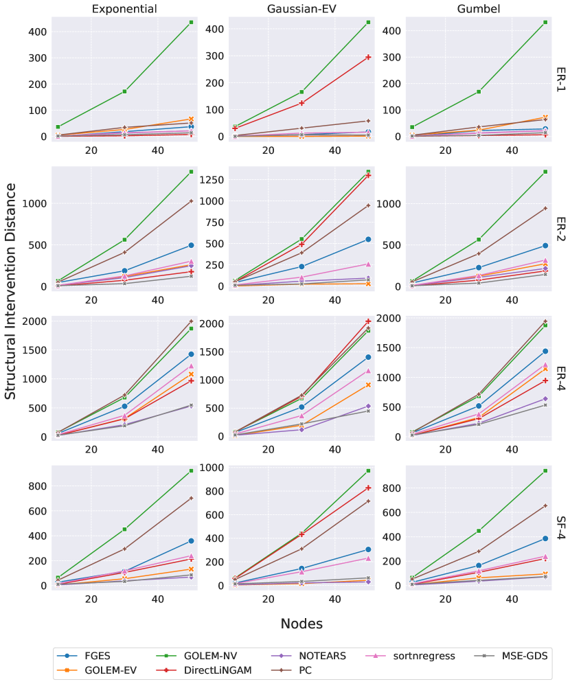
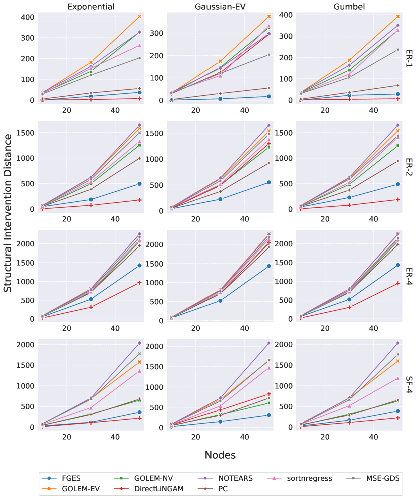
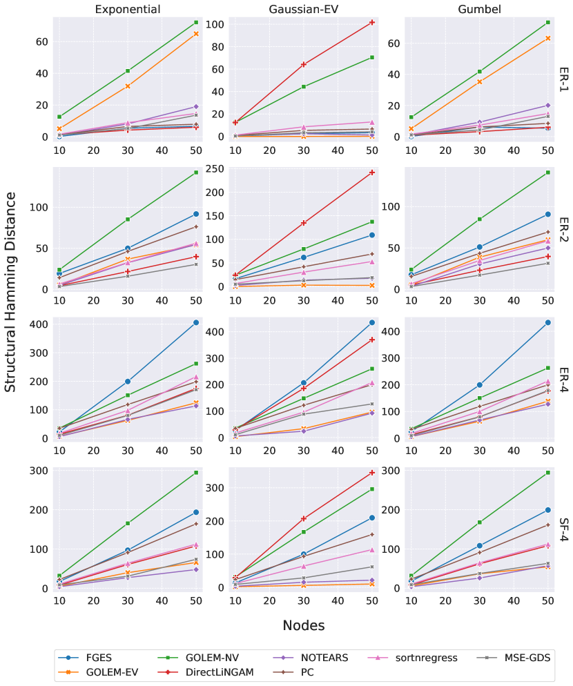
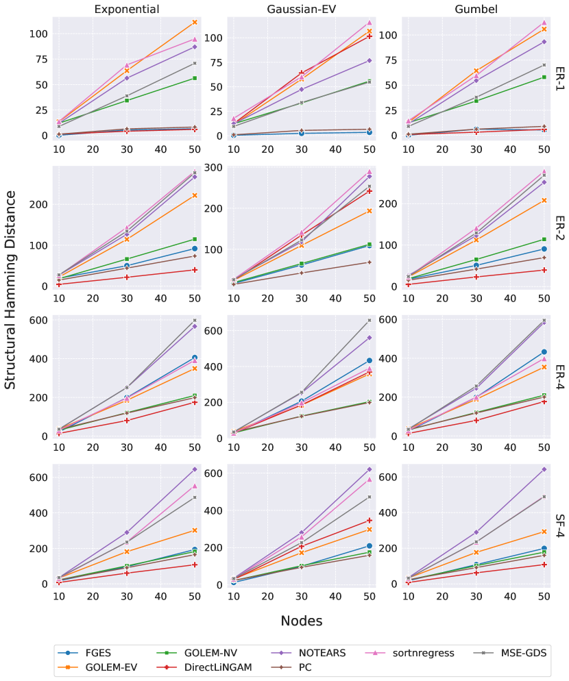
We compare the performance of the algorithms introduced in Section 2.3 on raw and standardized synthetic data. In our comparison, we distinguish between settings with different noise distributions, graph types, and graph sizes. Our experimental set-up follows those in Zheng et al. [2018], Ng et al. [2020] and we contribute results obtained repeating their experiments in Appendix K. We complement our and previous DAG-recovery results by additionally evaluating how well the DAG output by continous structure learning algorithms identifies the MEC of the ground-truth DAG.

4.1 Data Generation

We sample Erdös-Rényi (ER) [Erdős and Rényi, 1960] and Scale-Free (SF) [Barabási and Albert, 1999] graphs and the parameters for ANMs according to the simulation details in Table 1. For a graph specified as ER-$k$ or SF-$k$ with $d$ nodes, we simulate $dk$ edges. For every combination of parameters, we create a raw data instance and a standardized version that is de-meaned and re-scaled to unit variance. On standardized data, we have varsortability $v=\frac{1}{2}$ and the marginal variances hold no information about the causal ordering of the nodes. In all our experimental settings, varsortability averages above $0.94$ on the raw data scale (cf. Section G.1).

Table 1: Parameters for synthetic data generation.

Repetitions	10	Edge weights	iid  $\operatorname{Unif}((-2,-.5)\cup(.5,2))$
Graphs	ER-2, SF-2, SF-4	Noise distributions	Exponential, Gaussian, Gumbel
Nodes	$d\in\{10,30,50\}$	Noise standard deviations	$1$ (Gaussian-EV); iid  $\operatorname{Unif}(.5,2)$ (others)
Samples	$n=1000$

4.2 Evaluation

We evaluate performance using structural intervention distance (SID) [Peters and Bühlmann, 2015] and structural Hamming distance (SHD) between the recovered graph and ground truth. Additionally, we contribute a performance assessments of continuous structure learning algorithms in terms of the SID and SHD between the ground-truth MEC and the recovered MEC (PC, FGES) or the MEC identified by the recovered graph (NOTEARS, GOLEM). SID assesses in how far the recovered structure enables to correctly predict the effect of interventions. SHD measures the distance between the true and recovered graph by counting how many edge insertions, deletions, and reversals are required to turn the former into the latter. Since interventional distributions can consistently be estimated given only the causal ordering [Bühlmann et al., 2014], SID is less susceptible to arbitrary choices of edge pruning procedures and thresholds than SHD. Intuitively, SID prioritizes the causal order, while SHD prioritizes the correctness of individual edges. We follow common practices for edge thresholding and scoring (see Appendix K).

4.3 Performance on Raw Versus Standardized Data

We group our algorithms into combinatorial and continuous algorithms. We propose a novel baseline algorithm termed sortnregress which serves as a reference marking the performance achievable by directly exploiting marginal variances. We indicate its performance on standardized data as randomregress, since it amounts to choosing a random order and regressing each node on its predecessors. We use boxplots aggregating the performance achieved in the $10$ repetitions on raw and standardized data by each algorithm and create separate plots per noise type to account for identifiability and MLE specification differences. We show the results obtained for ER-2 graphs and Gaussian noise with non-equal variances in Figure 1. These results are representative of the results obtained for different graphs and noise distributions (cf. Appendix K). For the simulated settings, varsortability is high ($>0.94$) on the raw data scale (cf. Section G.1).

Recovery of ground-truth DAG
Recovery of ground-truth DAG’s Markov equivalence class

Figure 1: SID (left, lower is better) and SHD (right, lower is better) between recovered and ground-truth graphs (top) or Markov equivalence classes (bottom) for ER-2 graphs with 50 (top) or 10 (bottom) nodes and Gaussian-NV noise. The performance of sortnregress, which only exploits varsortability, matches that of the continuous methods NOTEARS and GOLEM.

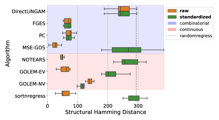
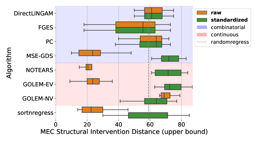
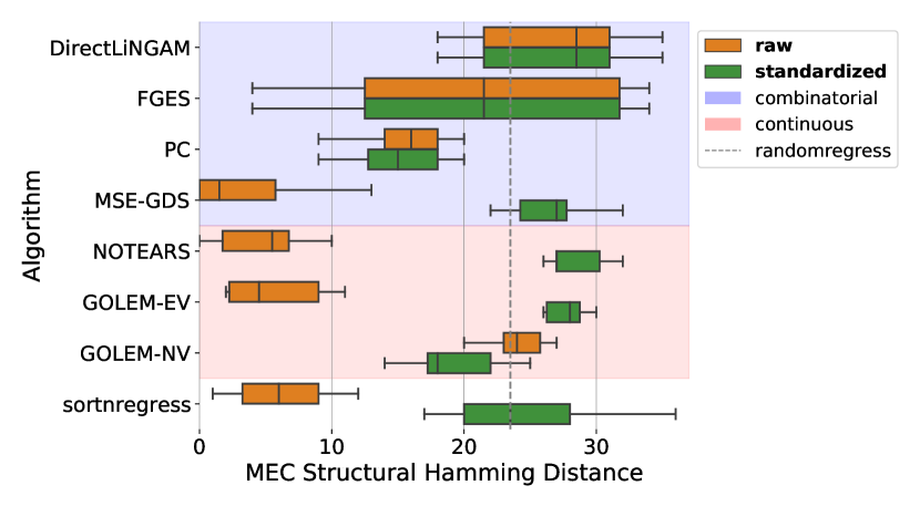
We observe that some algorithms are highly scale-sensitive and perform vastly different on raw and standardized data. The algorithms NOTEARS, MSE-GDS, GOLEM-EV are most affected – their performance is excellent on raw data but far worse on standardized data. Note that all of these rely on a loss function that revolves around the MSE. The performance of GOLEM-NV is also scale-sensitive but improves upon standardization. The direction of the effect of standardization is in line with the predictions by our gradient analysis in Section 3.4. Note that we initialize all algorithms with the empty graph since we are primarily interested in comparing the impact of standardization given equal starting conditions. On standardized data, an initialization of GOLEM-NV with the results of GOLEM-EV, as recommended by Ng et al. [2020], does not improve performance and may fail to converge. sortnregress achieves competitive performance on raw, and baseline performance on standardized data. It thus qualifies as diagnostic tool to highlight how much of a given causal structure learning task can be resolved by exploiting data scale and sorting nodes by their marginal variance.

In summary, the evidence corroborates our claim that the remarkable performance on raw data and the overall behavior upon standardization of the continuous structure learning algorithms may be driven primarily by high varsortability. On a real-world causal protein signaling dataset [Sachs et al., 2005] we measure a mean varsortability of $0.57$ (which is close to chance level at 0.5) with a standard deviation of $0.01$ across our bootstrapped samples and do not observe the consistent performance pattern described for synthetic data with high varsortability (cf. Appendix I).

5 Gaming Further Benchmarks

5.1 Orienting Causal Chains on Standardized Data

In order to design a causal discovery benchmark that does not favor methods that explicitly exploit marginal variances we may standardize the data or employ coefficient re-scaling schemes. Mooij et al. [2020], for example, propose a scale-harmonization by dividing each column $w_{j}=[w_{k\to j}]_{j=1,...,d}\in\mathbb{R}^{d}$ of the drawn adjacency matrices by $\sqrt{\|w_{j}\|^{2}+1}$ such that each variable would have comparable scale if all its direct parents were independently standard-normally distributed. However, this does not avoid the problem of potentially inadvertent patterns in simulated ANMs. Even after standardization or scale-harmonization, DAGs with previously high varsortability generate data with distinct covariance patterns that may be exploited.

In Appendix F we present an instructive example of a decision rule that can infer the orientation of a causal chain from raw, standardized, and scale-harmonized data with accuracy strictly greater than 50%. For a causal chain $X_{1}\to X_{2}\to...\to X_{d}$ where edge weights and noise terms are drawn iid we can decide between the two Markov-equivalent graphs $X_{1}\to X_{2}\to...\to X_{d}$ and $X_{1}\leftarrow X_{2}\leftarrow...\leftarrow X_{d}$ whith above-chance accuracy. The empirical results for varying chain-lengths and various edge-weight distribution are deferred to the appendix where we discuss the 3-variable chain in detail and illustrate that the phenomenon extends from finite-sample to the population setting.

The intuition is as follows. Consider data generated by $X_{1}\to X_{2}\to...\to X_{d}$ and the aim is to infer from standardized data whether $X_{1}\to...\to X_{d}$ or $X_{1}\leftarrow...\leftarrow X_{d}$. For data with high varsortability and comparable noise variance on the raw data scale it holds that the further downstream a node $X_{i}$ is in the causal chain, the stronger the variance of its parent $\operatorname{Var}(X_{i-1})$ contributes to its marginal variance $\operatorname{Var}(X_{i})=\operatorname{Var}(X_{i-1})+\operatorname{Var}(N_{i})$ relative to its noise variance $\operatorname{Var}(N_{i})$, and the stronger is it correlated with its parent. Thus, the sequence of regression coefficients, which in the standardized case amounts to $(\operatorname{Corr}(X_{i},X_{i+1}))_{i=1,...,d-1}$, tends to increase in magnitude along the causal order and decrease in the anti-causal direction. The proposed decision rule predicts the causal direction as the one in which the absolute values of the regression coefficients tend to increase. This chain orientation rule achieves above-chance performance on raw, standardized, and scale-harmonized data (cf. Appendix F).

5.2 Sorting by Variance in Non-Linear Settings

Varsortability may also be exploited in non-linear settings. Table 2 shows the results of sorting by marginal variance and filling in all edges from lower-variance nodes to higher-variance nodes in a non-linear setting. This variance sorting strategy is more naive than sortnregress and places no assumption on the functional form. The results are substantially better than random sorting and may therefore be a more informative baseline than commonly used random graphs. We do not show performance in terms of SHD, as our variance sorting baseline always yields a fully connected graph. Although the data generating process is not identical, we note that the improvement of our crude variance sorting over random sorting compares favorably to some of the improvements gained by more involved methods over random graphs as shown in Lachapelle et al. [2019, Table 1]. Our results indicate that exploiting varsortability may also deliver competitive results in non-linear settings.

Table 2: SID of naive baselines on non-linear data. Results on $1000$ observations of additive Gaussian process ANMs with noise variance 1 simulated as by Zheng et al. [2020] ($10$ repetitions each; average varsortability $\varv$ per graph type shown in parentheses).

Algorithm	Graph	ER-1	ER-4	SF-1	SF-4
	(average $\varv$)	($0.87$)	($0.95$)	($0.95$)	($0.98$)
variance sorting		$7.7\pm\phantom{0}5.72$	$25.2\pm 12.36$	$\phantom{0}1.9\pm 2.28$	$\phantom{0}7.6\pm 3.37$
random sorting		$27.9\pm 11.44$	$63.1\pm\phantom{0}8.10$	$22.3\pm 13.14$	$59.5\pm 7.32$

We find similarly high levels of varsortability for many non-linear functional relationships and graph parameters (cf. Section G.2). This begs the question how much other successful methods exploit varsortability, how they compare to non-linear nonparametric methods that leverage assumptions on the residual variances [Gao et al., 2020], and how they perform under data standardization. We encourage such an exploration in future work and suggest that varsortability and sortnregress or variance sorting should always be included in future benchmarks.

6 Discussion and Conclusion

We find that continuous structure learning methods are highly susceptible to data rescaling and some do not perform well without access to the true data scale. Therefore, scale-variant causal structure learning methods should be applied and benchmarked with caution, especially if the variables do not share a measurement scale or when the true scale of the data is unattainable. It is important to declare whether data is standardized prior to being fed to various structure learning algorithms.

Following the first release of the present paper, Kaiser and Sipos [2021] also independently reported the drop in performance of NOTEARS upon standardizing the data and presented a low-dimensional exemplary case. Beyond a reporting of impaired NOTEARS performance, we also analyze score-equivalent methods, provide exhaustive simulation experiments, and explain the phenomenon.

Our aim is to raise awareness of the severity with which scaling properties in data from simulated DAGs and causal additive models may distort algorithm performance. Increasing marginal variances can render scenarios identifiable, which may commonly not be expected to be so—for example the Gaussian case with non-equal variances. We therefore argue that varsortability should be taken into account for future benchmarking. Yet, with any synthetic benchmark there remains a risk that the results are not indicative of algorithm performance on real data. Our results indicate that current structure learning algorithms may perform within the range of naive baselines on real-world datasets.

The theoretical results of our paper are limited to the setting of linear ANMs. Additionally, our conjecture regarding the importance of the first gradient steps, and with it a rigorous causal explanation for the learning behavior of different continuous algorithms and corresponding score functions remain open and require further research to be settled. Our empirical findings indicate that causal discovery benchmarks can be similarly gamed on standardized data and in non-linear settings, but further research is needed to confirm this. We focus on a specific subset of algrorithms, the impact of patterns in benchmarking data on a wider class of algorithms and score functions remains to be explored.

Varsortability arises in many ANMs and the marginal variances increase drastically along the causal order, at least in common simulation settings. This begs the question what degree of varsortability can be observed or assumed in real-world data. If the marginal variances carry information about the causal order, our results suggest that it can and should be leveraged for structure learning. Otherwise, our contribution motivates future research into representative benchmarks and may put the practical applicability of the additive noise assumption into question.

Acknowledgements

We thank Jonas M. Kübler, Jonas Peters, and Sorawit Saengkyongam for helpful discussions and comments. SW was supported by the Carlsberg Foundation.

References

Appendix

Appendix A Varsortability in the Two-Node Case

Consider the following ground truth and two competing linear acyclic models:

Ground-truth model:

$$A :=N_{A}$$

$$B :=wA+N_{B}$$

Model M1) “$A\to B$”:

$$\widehat{A} =0$$

$$\widehat{B} =\widehat{w}A$$

Model M2) “$A\leftarrow B$”:

$$\widehat{A} =\widehat{v}B$$

$$\widehat{B} =0$$

where $w\neq 0$, $N_{A}$ and $N_{B}$ are independent zero-centred noise terms that follow some distributions with non-vanishing corresponding variance $V_{A}$ and $V_{B}$. The model parameters $\widehat{w}=\frac{\operatorname{Cov}(A,B)}{\operatorname{Var}(A)}=w$ and $\widehat{v}=\frac{\operatorname{Cov}(A,B)}{\operatorname{Var}(B)}=\frac{wV_{A}}{\operatorname{Var}(B)}$ are the corresponding ordinary least-squares linear regression coefficients.

We evaluate in which cases the true model M1 obtains a smaller MSE than the wrong model M2, to decide if and under which conditions a MSE-based orientation rule recovers the ground-truth edge direction:

$$\operatorname{MSE}\left(M1\right) <\operatorname{MSE}\left(M2\right)$$

$$\iff \operatorname{Var}(A)+\operatorname{Var}(B-\widehat{w}A) <\operatorname{Var}(A-\widehat{v}B)+\operatorname{Var}(B)$$

$$\iff \operatorname{Var}(A)+\operatorname{Var}\left((wN_{A}+N_{B})-wN_{A}\right) <\operatorname{Var}\left({N_{A}-\frac{wV_{A}}{\operatorname{Var}(B)}(wN_{A}+N_{B})}\right)+\operatorname{Var}(B)$$

$$\iff V_{A}+V_{B} <\frac{V_{A}V_{B}}{\operatorname{Var}(B)}+w^{2}V_{A}+V_{B}$$

$$\iff 0 <V_{A}\left(\frac{V_{B}}{\operatorname{Var}(B)}-1\right)+w^{2}V_{A}$$

$$\iff 0 <\frac{-w^{2}V_{A}}{\operatorname{Var}(B)}+w^{2}$$

$$\iff V_{A} <\operatorname{Var}(B)$$

$$\iff (1-w^{2})V_{A} <V_{B}$$

For error variances $V_{A}\leq V_{B}$ and any non-zero edge weight $w$, the MSE-based inference is correct. This resembles known scale-based identifiability results based on equal or monotonically increasing error variances [Peters and Bühlmann, 2014, Park, 2020].

Appendix B Derivation of Lower Bound on Pairwise Varsortability

Let $A$ and $B$ be any two nodes in the sampled graph with edge $A\overset{w}{\to}B$, noise terms $N_{A},N_{B}$, and without common ancestors and no other directed path from $A$ to $B$. When sampling edge coefficients and noise variances randomly for the simulation of ANMs, distributions are incurred over the variances of $A$ and $B$ across those simulated ANMs. Let edge weights be sampled as $[W_{x\to y}]_{x,y=1,...,d}\sim\mathbb{P}_{W}$, and noise variances be sampled as $[S^{2}_{N_{y}}]_{y=1,...,d}\sim\mathbb{P}_{S^{2}}$. Across simulations, the marginal variances of $A$ and $B$ are transformations of $S$ and $W$ and themselves random variables denoted as $V_{A}$ and $V_{B}$. The marginal variance $V_{Y}$ of any node $Y$ depends on its noise variance and the additional variance incurred by predecessor nodes given as $\sum_{X\in\operatorname{PA}\left(Y\right)}W_{X\to Y}^{2}V_{X}$. We can therefore bound the probability for the variable pair $(A,B)$ to be varsortable from below via

$$\operatorname{P}[{V_{A}<V_{B}}]= \operatorname{P}\left[V_{A}<\left({W_{AB}^{2}V_{A}+\sum_{X\in\operatorname{PA}\left(B\right)\setminus\{A\}}W_{XB}^{2}V_{X}+S_{N_{B}}^{2}}\right)\right]$$

$$\geq \operatorname{P}[V_{A}<W_{AB}^{2}V_{A}+S_{N_{B}}^{2}]$$

where equality holds if $A$ is the only parent of $B$ contributing to $B$’s marginal variance.

In common benchmarks, edge weights are drawn independently according to $\mathbb{P}_{W}\sim\otimes_{k,j=1,...,d}\operatorname{Unif}((-2,-.5)\cup(.5,2))$ and noise standard deviations are drawn iid $S_{N_{j}}\sim\operatorname{Unif}(.5,2)$.

Appendix C Varsortability and Identifiability by Conditional Noise Variances

While closely related, varsortability is not equivalent to the identifiability conditions laid out in Theorem 4, Park [2020], (henceforth referred to as “Theorem 4”). We prove this by providing two examples. In Section C.1 part A) of the conditions in Theorem 4 is satisfied, while varsortability does not hold. In Section C.2 varsortability holds but neither part A) nor part B) of Theorem 4 are satisfied.

C.1 Park, 2020, Theorem 4 conditions satisfied without varsortability

Consider the following ground-truth model with unique causal order $A,B,C$:

$$A :=N_{A}$$

$$B :=\beta_{A\to B}A+N_{B}=1A+N_{B}$$

$$C :=\beta_{B\to C}B+N_{C}=\sqrt{\frac{2}{3}}B+N_{C}$$

where $N_{A},N_{B},N_{C}$ are jointly independent zero-centred noise terms with respective variances $\sigma_{A}^{2}=4,\sigma_{B}^{2}=2,\sigma_{C}^{2}=1$. The marginal variances are $\operatorname{Var}(A)=4\ <\operatorname{Var}(C)=5\ <\operatorname{Var}(B)=6$. Our example resembles the examples in Section 3.1 of Park [2020]. We can verify the three conditions for part A) of Theorem 4:

$$(A1)\quad \sigma_{A}^{2}<\sigma_{B}^{2}+\beta_{A\to B}^{2}\sigma_{A}^{2},$$

$$(A2)\quad \sigma_{B}^{2}<\sigma_{C}^{2}+\beta_{B\to C}^{2}\sigma_{B}^{2},$$

$$(A3)\quad \sigma_{A}^{2}<\sigma_{C}^{2}+\beta_{B\to C}^{2}\sigma_{B}^{2}+\beta_{A\to B}^{2}\beta_{B\to C}^{2}\sigma_{A}^{2}$$

Inserting the values from above, we obtain

$$(A1)\quad 4<2+1\cdot 4,$$

$$(A2)\quad 2<1+\frac{2}{3}\cdot 2,$$

$$(A3)\quad 4<1+\frac{2}{3}\cdot 2+1\cdot\frac{2}{3}\cdot 4.$$

Our result verifies that identifiability is given as per Theorem 4 in Park [2020], while the order of increasing marginal variances is not in complete agreement with the causal order and varsortability is not equal to $1$.

C.2 Varsortability without Park, 2020, Theorem 4 conditions satisfied

Consider the following ground-truth model with unique causal order $A,B,C$:

$$A :=N_{A}$$

$$B :=\beta_{A\to B}A+N_{B}=A+N_{B}$$

$$C :=\beta_{A\to C}A+\beta_{B\to C}B+N_{C}=\frac{1}{\sqrt{2}}A+\frac{1}{\sqrt{2}}B+N_{C}$$

where $N_{A},N_{B},N_{C}$ are jointly independent zero-centred noise terms with respective variances $\sigma_{A}^{2}=4,\sigma_{B}^{2}=3,\sigma_{C}^{2}=1$. The marginal variances are $\operatorname{Var}(A)=4\ <\operatorname{Var}(B)=7\ <\operatorname{Var}(C)=10.5$. We now verify, that for both case A) and B) in Theorem 4 of Park [2020] at least one of the inequality constraints is violated.

One of the three conditions in A) is

$$\sigma_{B}^{2}<\sigma_{C}^{2}+\beta_{B\to C}^{2}\sigma_{B}^{2},$$

while for the above model we have

$$3\nless 1+\frac{1}{2}\cdot 3.$$

One of the three conditions in B) is

$$\frac{\sigma_{C}^{2}}{\sigma_{B}^{2}}>(1-\beta_{B\to C}^{2}),$$

while for the above model we have

$$\frac{1}{3}\ngtr(1-\frac{1}{2}).$$

For both criteria A) and B) in Theorem 4 at least one of the inequalities is not satisfied. We thus verify that even if identifiability is not given as per the sufficient conditions in Theorem 4, Park [2020], varsortability may still render the causal order identifiable.

Appendix D Algorithms

DirectLiNGAM

is a method for learning linear non-Gaussian acyclic models [Shimizu et al., 2011]. It recovers the causal order by iteratively selecting the node whose residuals are least dependent on any predecessor node. In a strictly non-Gaussian setting, DirectLiNGAM is guaranteed to converge to the optimal solution asymptotically within a small fixed number of steps and returns a DAG. We use the implementation provided by the authors. We deliberately keep the default of a least-angle regression penalized by the Bayesian Informaion Criterion. We find that this penalty strikes a good balance between SID and SHD performance. Cross-validated least-angle regression performs better in terms of SID but poorer in terms of SHD.

PC

[Spirtes and Glymour, 1991] is provably consistent in estimating the Markov equivalence class of the true data-generating graph if the causal Markov and faithfulness assumptions hold. The algorithm returns a completed partially directed acyclic graph (CPDAG). For computational reasons, we refrain from computing the lower and upper bounds of the SID for comparing CPDAGS with the ground-truth DAG as proposed by Peters and Bühlmann [2015]. Instead, we adopt the approach by Zheng et al. [2018] and resolve bidirectional edges favorably to obtain a DAG. We use the implementation in the Tetrad package Ramsey et al. [2018].

FGES

is an optimized version of the fast greedy equivalence search algorithm developed by Meek [1997], Chickering [2002b]. Under causal Markov and faithfulness assumptions, it is provably consistent for estimating the Markov equivalence class of the true data-generating graph. The algorithm returns a CPDAG, which we resolve favorably to obtain a DAG. We use the implementation in the Tetrad package [Ramsey et al., 2018].

MSE-GDS

is a greedy DAG search procedure with a MSE score criterion. We implement MSE-GDS following other GDS procedures, for example, as described by Peters and Bühlmann [2014, Section 4], but use the MSE as score criterion instead of a likelihood- or BIC-based score criterion. For simplicity and computational ease, we consider a smaller search space and greedily forward-search over new edge insertions only instead of greedily searching over all neighbouring DAGs obtainable by edge insertions, removals, and deletions. For the linear setting, linear regression is used to determine the edge weights and the corresponding MSE-score for a given graph. For the non-linear setting, support vector regression can be used instead. The algorithm returns a DAG.

NOTEARS

is a score-based method that finds both structure and parameters simultaneously by continuous optimization [Zheng et al., 2018]. The optimization formulation is based on the mean squared error and includes a sparsity penalty parameter $\lambda$ and a differentiable acyclicity constraint:

$$\operatorname*{\arg\!\min}_{W\in\mathbb{R}^{d\times d}}\quad\operatorname{MSE}_{\mathbf{X}}\left(W\right)+\lambda\|W\|_{1}\quad\textrm{s.t.}\quad\operatorname{tr}(\exp(W\odot W))-d=0.$$

The algorithm returns a DAG. We use the implementation provided by the authors. Throughout all our experiments we use NOTEARS over NOTEARS-L1 (setting $\lambda=0$), following the findings of Zheng et al. [2018, Tables 1 and 2, Figure 3], which suggest regularization only for samples smaller than the $n=1000$ we use throughout.

GOLEM

combines a soft version of the differentiable acyclicity constraint from Zheng et al. [2018] with a MLE objective [Ng et al., 2020]. The authors propose a multivariate Gaussian MLE for equal (EV) or unequal (NV) noise variances and optimize

$$\operatorname*{\arg\!\min}_{W\in\mathbb{R}^{d\times d}}\quad\mathcal{\widetilde{L}}(W,\mathbf{X})-\log(|\det(I-W)|)+\lambda_{1}\|W\|_{1}+\lambda_{2}(\operatorname{tr}(\exp(W\odot W))-d)$$

where $\mathcal{\widetilde{L}}$ is either

$$\mathcal{\widetilde{L}}_{EV}(W,\mathbf{X}) =\frac{d}{2}\left(\mathcal{L}_{EV}(W,\mathbf{X})+\log(n)\right)=\frac{d}{2}\log(n\operatorname{MSE}_{\mathbf{X}}\left(W\right))\text{, or}$$

$$\mathcal{\widetilde{L}}_{NV}(W,\mathbf{X}) =\frac{1}{2}\left(\mathcal{L}_{NV}(W,\mathbf{X})+d\log(n)\right)=\frac{1}{2}\sum_{j=1}^{d}\log(n\operatorname{MSE}_{j}\left(w_{j}\right)).$$

We use the implementation and hyperparameters provided by the authors. We train for $10^{4}$ episodes as we found that half of that suffices to ensure convergence. Notably, we do not perform pretraining for our version of GOLEM-NV.

sortnregress

is implemented as shown in Section H.1. We find that a least-angle regression penalized by the Bayesian Information Criterion strikes a good balance between SID and SHD performance.

Appendix E The Subtle Interplay Between Marginal Variance and Gradient Directions

We describe observations about the gradients involved in the optimization procedures of NOTEARS and GOLEM-EV/-NV. We present an instructive example in Section E.1 and provide some intuition about how the adjacency matrix changes throughout the optimization. For convenience and reference we provide gradients of the individual terms involved in the respective objective functions (cf. Section E.2). In Section E.3 we argue why the nodes’ residual variances for the first gradient steps in an unconstrained optimization of MSE- or log-MSE-EV-based (GOLEM-EV) objective functions with acyclicity penalties tend to follow the same ordering as the nodes’ marginal variances. We analyze gradient symmetry and asymmetry in GOLEM-EV/-NV’s gradient descent optimization under varsortability in Section E.4. While the intuition for small step size gradient-based unconstrained optimization partially carries over to the NOTEARS optimization procedure, here the interplay between varsortability and gradient directions is intricate due to a constrained optimization that is solved via the augmented Lagrangian method and dual descent with line-search instead of gradient descent as used in GOLEM [Zheng et al., 2018] (cf. Section E.5).

The heuristic arguments presented here are preliminary and aim to provide intuition. The optimization behaviour also heavily depends on the implementation of the optimization routine. For example, the original implementation of NOTEARS fixes the diagonal of $W$ at zero and leverages curvature information (L-BFGS-B), while GOLEM updates all entries of $W$ and employs learning rate optimizers. Future research is required to determine how precisely continuous structure learning algorithms achieve state-of-the-art results on highly varsortable data and, given our observations, we expect explanations to be specific to individual algorithms and their distinct implementations.

E.1 Example

The following example considers the population limit and illustrates a few intuitions about gradient based optimization and varsortability. Consider data is generated according to

$$\begin{pmatrix}X\\ Y\end{pmatrix}=\begin{pmatrix}0&\beta\\ 0&0\end{pmatrix}^{\top}\begin{pmatrix}X\\ Y\end{pmatrix}+\begin{pmatrix}N_{X}\\ N_{Y}\end{pmatrix}$$

where $N_{X}$ and $N_{Y}$ are independently normally distributed with standard deviations $\sigma_{N_{X}}$ and $\sigma_{N_{Y}}$. Here, varsortability $\varv=1$ and $1=\operatorname{Var}{X}<\operatorname{Var}{Y}=2$.

Initializing the weight matrix at the zero matrix, the gradient of the population MSE is

$$-2\begin{pmatrix}\operatorname{Var}(X)&\operatorname{Cov}(X,Y)\\ \operatorname{Cov}(Y,X)&\operatorname{Var}(Y)\end{pmatrix}=-2\begin{pmatrix}\sigma_{N_{X}}^{2}&\beta\sigma_{N_{X}}^{2}\\ \beta\sigma_{N_{X}}^{2}&\beta^{2}\sigma_{N_{X}}^{2}+\sigma_{N_{Y}}^{2}\end{pmatrix}$$

(see also Section E.2). The models for $X$ and $Y$ after a first gradient descent step of step size $\eta$ are

$$\widehat{X} =2\eta(\sigma_{N_{X}}^{2}X+\beta\sigma_{N_{X}}^{2}Y)$$

$$\widehat{Y} =2\eta(\beta\sigma_{N_{X}}^{2}X+(\beta^{2}\sigma_{N_{X}}^{2}+\sigma_{N_{Y}}^{2})Y)$$

If the diagonal of the weight matrix is clamped to $0$ throughout the optimization, the terms corresponding to self-loops ($2\eta\sigma_{N_{X}}^{2}X$ in $\widehat{X}$ and $(\beta^{2}\sigma_{N_{X}}^{2}+\sigma_{N_{Y}}^{2})Y$ in $\widehat{Y}$) are dropped above. This is the case in the original implementation of NOTEARS, where the unconstrained subproblem is optimized via L-BFGS-B with identity bounds on the diagonal entries of $W$.

Below we visualize $\operatorname{Var}(X-\widehat{X})$ (residual variance in $X$), $\operatorname{Var}(Y-\widehat{Y})$ (residual variance in $Y$), and the MSE $\operatorname{Var}(X-\widehat{X})+\operatorname{Var}(Y-\widehat{Y})$, for varying step sizes $\eta$ of the first gradient step where we exemplary choose $\beta=\sigma_{N_{X}}=\sigma_{N_{Y}}=1$.

Since the residual variances change continuously for increasing step sizes, the residual variances follow the order of the marginal variances for small step sizes (cf. also Section E.3). Since in GOLEM we solve an unconstrained optimization problem by gradient descent (with small step size and learning rate), the order of residual variances tends to remain unchanged during the first optimization steps. The order of the residual variances may swap relative to the order of marginal variances, though, if line-search is employed to determine the step size that minimizes the MSE-objective. This is the case in NOTEARS, where the MSE is minimized by a dual descent routine with increasing weight on the acyclicity penalty term. Here, the first symmetric update of the weight matrix occurs with a large step size that minimizes the MSE (minimum of the green curves in above plots). The ordering of the resulting residual variances is less obvious. In the above example, if the diagonal terms of the weight matrix are updated as well (left), the residual variance order after the first gradient step is opposite to the marginal variance order. If the diagonal entries are clamped at $0$ (as is the case in NOTEARS and corresponding to the setting shown on the right), the first gradient step in the above example leads to a scenario where the residual variance order follows the marginal variance order and where the resulting edge weight for the direction $X\leftarrow Y$ overshoots the optimum, that is, the blue curve’s minimum is attained for a smaller step size than the green curve’s minimum. The intuition is as follows: If we minimize the MSE the step size calibrates a trade-off between residual variances in the different nodes; the high marginal variance nodes dominate the MSE such that the step size that minimizes the MSE may result in ill-chosen edge weights for the edges incoming into low-variance nodes. In the next optimization step, the gradient of the MSE loss for the edge $X\to Y$ pushes towards increasing that edge weight, while it pushes for decreasing the edge weight $X\leftarrow Y$ (besides a gradient contribution from the acyclicity constraint). As a result, the edge weights for $X\to Y$ and $X\leftarrow Y$ are equal after the first step of NOTEARS, but better calibrated for the direction from low- to high-variance nodes, which here corresponds to the correct edge $X\to Y$. In the subsequent optimization step, decreasing the edge weight $X\leftarrow Y$ is favored both by the MSE gradient and the acyclicity penalty, while for the correct edge $X\to Y$ the MSE gradient pushes to further increasing the edge. Intuitively, if one needs to cut one of the two edges to avoid cycles, it is “cheaper” in MSE to cut the wrong edge $X\leftarrow Y$ from a high- to low-variance node.

E.2 Stepwise Gradient Derivation

MSE

For $\mathbf{X}\in\mathbb{R}^{n\times d}$, the gradient of $\operatorname{MSE}_{\mathbf{X}}\left(W\right)=\frac{1}{n}\|\mathbf{X}-\mathbf{X}W\|_{2}^{2}$ is

$$\nabla_{W}\operatorname{MSE}_{\mathbf{X}}\left(W\right) =\frac{1}{n}\nabla_{W}\left(\operatorname{Tr}[\mathbf{X}^{\top}\mathbf{X}]-\operatorname{Tr}[W^{\top}\mathbf{X}^{\top}\mathbf{X}]-\operatorname{Tr}[\mathbf{X}^{\top}\mathbf{X}W]+\operatorname{Tr}[W^{\top}\mathbf{X}^{\top}\mathbf{X}W]\right)$$

$$=\frac{1}{n}\left(-\mathbf{X}^{\top}\mathbf{X}-\mathbf{X}^{\top}\mathbf{X}+\mathbf{X}^{\top}\mathbf{X}W+\mathbf{X}^{\top}\mathbf{X}W\right)$$

$$=-\frac{2}{n}\left(\mathbf{X}^{\top}\mathbf{X}-\mathbf{X}^{\top}\mathbf{X}W\right)$$

$$=-\frac{2}{n}\mathbf{X}^{\top}(\mathbf{X}-\mathbf{X}W)$$

$$\propto\mathbf{X}^{\top}(\mathbf{X}-\mathbf{X}W)$$

If $W$ is polynomial in $\mathbf{X}^{\top}\mathbf{X}$, $\nabla_{W}\operatorname{MSE}_{\mathbf{X}}\left(W\right)$ is symmetric. $\nabla_{W}\operatorname{MSE}_{\mathbf{X}}\left(\mathbf{0}_{d\times d}\right)=-\frac{2}{n}\mathbf{X}^{\top}\mathbf{X}$.

GOLEM-EV

The gradient of the unnormalized negative likelihood-part of the GOLEM-EV objective denoted as $\mathcal{\widetilde{L}}_{EV}(W,\mathbf{X})$ is

$$\nabla_{W}\mathcal{\widetilde{L}}_{EV}(W,\mathbf{X}) =\frac{d}{2}\nabla_{W}\log(n\operatorname{MSE}_{\mathbf{X}}\left(W\right))$$

$$=\frac{d}{2}\frac{1}{\operatorname{MSE}_{\mathbf{X}}\left(W\right)}\nabla_{W}\operatorname{MSE}_{\mathbf{X}}\left(W\right)$$

$$\propto\frac{1}{\operatorname{MSE}_{\mathbf{X}}\left(W\right)}\mathbf{X}^{\top}(\mathbf{X}-\mathbf{X}W)$$

If $W$ is polynomial in $\mathbf{X}^{\top}\mathbf{X}$, $\nabla_{W}\mathcal{\widetilde{L}}_{EV}(W,\mathbf{X})$ is symmetric. $\nabla_{W}\mathcal{\widetilde{L}}_{EV}(\mathbf{0}_{d\times d},\mathbf{X})=-\frac{d}{\|\mathbf{X}\|_{2}^{2}}\mathbf{X}^{\top}\mathbf{X}$.

GOLEM-NV

The gradient of the unnormalized negative likelihood-part of the GOLEM-NV objective denoted as $\mathcal{\widetilde{L}}_{NV}(W,\mathbf{X})$ is

$$\nabla_{W}\mathcal{\widetilde{L}}_{NV}(W,\mathbf{X}) =\frac{1}{2}\sum_{j=1}^{d}\nabla_{W}\log(n\operatorname{MSE}_{j}\left(w_{j}\right))$$

$$=\left[-\frac{1}{n\operatorname{MSE}_{j}\left(w_{j}\right)}\mathbf{X}^{\top}(x_{j}-\mathbf{X}w_{j})\right]_{j=1,...,d}$$

$$\propto\left[\frac{\mathbf{X}^{\top}(x_{j}-\mathbf{X}w_{j})}{\operatorname{MSE}_{j}\left(w_{j}\right)}\right]_{j=1,...,d}$$

For the zero matrix, we have $\nabla_{W}\mathcal{\widetilde{L}}_{NV}(\mathbf{0}_{d\times d},\mathbf{X})=-\mathbf{X}^{\top}\mathbf{X}\operatorname{diag}\left(\|x_{1}\|_{2}^{-2},...,\|x_{d}\|_{2}^{-2}\right)$.

We focus on the gradients of $\operatorname{MSE}$, $\mathcal{L}_{EV}$, and $\mathcal{L}_{NV}$ since l1 penalty, acyclicity penalty $h$, LogDet term, and exact scaling of $\mathcal{\widetilde{L}}_{EV}$ and $\mathcal{\widetilde{L}}_{NV}$ play a subordinate role at the zero initialization, where the LogDet gradient has zero off-diagonals and $\nabla_{W}h$ vanishes:

The LogDet in GOLEM-EV and GOLEM-NV

$\operatorname{LogDet}(W)=\log(\operatorname{det}(I-W))$ has gradient

$$\nabla_{W}\operatorname{LogDet}(W)=-(I-W)^{-\top}$$

and vanishes when $W$ is the adjacency matrix of a DAG [Ng et al., 2020]. If $W$ is symmetric, $\nabla_{W}\operatorname{LogDet}(W)$ is symmetric. For the zero matrix, we have $\nabla_{W}\operatorname{LogDet}(\mathbf{0}_{d\times d})=-I$.

Acyclicity Penalty/Constraint

The function $h(W)=\operatorname{tr}(\exp(W\odot W))-d$ has gradient $\nabla_{W}h(W)=\exp(W\odot W)^{\top}\odot 2W$. The $h(W)\!\!=\!\!0$-level set characterizes adjacency matrices of DAGs [Zheng et al., 2018]. If $W$ is symmetric, $\nabla_{W}h(W)$ is symmetric. For the zero matrix, we have $h(\mathbf{0}_{d\times d})=0$ and $\nabla_{W}h(\mathbf{0}_{d\times d})=\mathbf{0}_{d\times d}$.

E.3 Increasing Marginal and Residual Variances

We observe a strong positive correlation between the ordering by marginal variance and the ordering by residual variance after the first gradient step when minimizing a MSE- or likelihood-based objective function via gradient descent with small step size (as in GOLEM-EV/-NV). For small step sizes and learning rates, marginal variance order and residual variance order are perfectly aligned for the first few optimization steps. Here we argue for a MSE-based loss function why the residual variance follows the order of increasing marginal variance after the first optimisation step with sufficiently small step size. Future work may investigate subsequent optimisation steps and the non-MSE terms of the objective functions.

Consider the data matrix $\mathbf{X}\in\mathbb{R}^{n\times d}$. Without loss of generality, we assume the columns are zero-centred and ordered such that the sequence of diagonal entries $\operatorname{diag}(\mathbf{X}^{\top}\mathbf{X})$ is weakly monotonically increasing. The diagonal entries $\operatorname{diag}(\mathbf{X}^{\top}\mathbf{X})$ correspond to ($n$-times) the marginal variances at step $0$. After the first gradient step with step size $\alpha$ in direction $-\nabla_{W}\operatorname{MSE}_{\mathbf{X}}\left(\mathbf{0}_{d\times d}\right)=\frac{2}{n}\mathbf{X}^{\top}\mathbf{X}$ (cf. Section E.2) the vector of ($n$-times) the residual variances is

$$\mathbf{R} =\operatorname{diag}\left([\mathbf{X}-a\mathbf{X}\mathbf{X}^{\top}\mathbf{X}]^{\top}[\mathbf{X}-a\mathbf{X}\mathbf{X}^{\top}\mathbf{X}]\right)$$

$$=\operatorname{diag}\left(\mathbf{D}\right)-2a\operatorname{diag}\left(\mathbf{D}^{2}\right)+a^{2}\operatorname{diag}\left(\mathbf{D}^{3}\right)$$

where $\mathbf{D}=\mathbf{X}^{\top}\mathbf{X}$ and $a=\frac{2}{n}\alpha$. For each coordinate $i$ the residual variance $\mathbf{R}_{i}$ is a continuous function in $a$ (and $\alpha$). For $a=0$ and every $i\in[1,...,d-1]$ we have $\mathbf{R}_{i+1}-\mathbf{R}_{i}=\mathbf{D}_{i+1}-\mathbf{D}_{i}\geq 0$ with strict inequality if the variable pair $i,i+1$ is varsortable. Due to continuity, for any pair of variables with unequal marginal variances, there exists a sufficiently small step size to ensure that the resulting residual variances follow the same order as the marginal variances.

E.4 Gradient Asymmetry

We combine what we laid out in Section E.2.

The GOLEM-EV optimization problem is

$$\operatorname*{\arg\!\min}_{W}\mathcal{\widetilde{L}}_{EV}(W,\mathbf{X})-\operatorname{LogDet}(W)+\lambda_{1}\|W\|_{1}+\lambda_{2}h(W)$$

with the following gradient of the objective function

$$-\frac{d}{n\operatorname{MSE}_{\mathbf{X}}\left(W\right)}\mathbf{X}^{\top}(\mathbf{X}-\mathbf{X}W)+(I-W)^{-\top}+\lambda_{1}W\oslash|W|+\lambda_{2}\exp(W\odot W)^{\top}\odot 2W$$

which at zero reduces to

$$-\frac{d}{\|\mathbf{X}\|_{2}^{2}}\mathbf{X}^{\top}\mathbf{X}+I.$$

The GOLEM-NV optimization problem is

$$\operatorname*{\arg\!\min}_{W}\mathcal{\widetilde{L}}_{NV}(W,\mathbf{X})-\operatorname{LogDet}(W)+\lambda_{1}\|W\|_{1}+\lambda_{2}h(W)$$

with the following gradient of the objective function

$$\left[-\frac{1}{n\operatorname{MSE}_{j}\left(w_{j}\right)}\mathbf{X}^{\top}(x_{j}-\mathbf{X}w_{j})\right]_{j=1,...,d}+(I-W)^{-\top}+\lambda_{1}W\oslash|W|+\lambda_{2}\exp(W\odot W)^{\top}\odot 2W$$

which at zero reduces to

$$-\mathbf{X}^{\top}\mathbf{X}\operatorname{diag}(\|x_{1}\|_{2}^{-2},...,\|x_{d}\|_{2}^{-2})+I.$$

The gradient in GOLEM-EV is symmetric at $\mathbf{0}_{d\times d}$ at the first gradient descent step, but not in general for later steps. The gradient in GOLEM-NV is in general not symmetric and at $\mathbf{0}_{d\times d}$ (at the first gradient descent step) the gradients for edges incoming into a node are inversely scaled by its marginal variance; consequently, for weights $w_{i\to j}$ and $w_{j\to i}$ of opposing edges the first gradient step is larger magnitude for the direction with lower-variance end-note and $w_{i\to j}$ is preferred over $w_{j\to i}$ if the variance of $X_{i}$ is higher than that of $X_{j}$. Under high-varsortability, the first GOLEM-NV gradient step thus tends to favor edges in anti-causal direction over those in causal direction.

E.5 NOTEARS

The NOTEARS optimization problem is $\operatorname*{\arg\!\min}_{W}\frac{1}{2}\operatorname{MSE}_{\mathbf{X}}\left(W\right)\text{ s.t. }h(W)=0$ which is solved via the augmented Lagrangian method and dual descent [Zheng et al., 2018] (we omit the penalty term for the NOTEARS-l1 variant). In the original implementation, the algorithm is initialized at $\mathbf{0}_{d\times d}$ and the diagonal of $W$ is not updated but fixed to zero (this amounts to dual projected descent, where the adjacency matrix is projected onto the matrices with zero diagonal at each step avoiding self-loops per fiat).

The augmented Lagrangian

$$\frac{1}{2}\operatorname{MSE}_{\mathbf{X}}\left(W\right)+\frac{\rho}{2}h(W)^{2}+\alpha h(W)$$

has gradient

$$-\frac{1}{n}\mathbf{X}^{\top}(\mathbf{X}-\mathbf{X}W)+(\rho h+\alpha)\left(\exp(W\odot W)^{\top}\odot 2W\right)$$

which at zero reduces to

$$-\frac{1}{n}\mathbf{X}^{\top}\mathbf{X}$$

The step size of the first gradient step in direction $\propto\mathbf{X}^{\top}\mathbf{X}$ is optimized by line-search to minmize the overall MSE. As seen in the example in Section E.1, the residual variances may or may not follow the order of the marginal variances after this first step due to the step size being larger than the small step size that would ensure agreement between the orders (cf. Section E.3). Nonetheless, the step size optimized by line-search aims to optimize the overall MSE which tends to favor a better fit for edges incoming into nodes with high-marginal variance. As a result, the first gradient step results in edge weights that are better calibrated for edges incoming into high-marginal variance nodes than into low-marginal variance nodes. In subsequent steps of the dual ascent procedure with increasing acyclicity penalty, the reduction of overall MSE stands at odds with satisfying the DAG constraints; it is then more costly in terms of MSE to change the weights for edges into high-marginal nodes than into low-marginal nodes such that predominantly the edges into low-variance nodes tend to be removed to eventually satisfy the acyclicity constraint. Under high varsortability, this amounts to a preference for causal edges.

Appendix F Standardization Is Not Enough and Regression Coefficients Tend to Increase Along the Causal Order

Code to reproduce the calculations and results in this section is available at https://github.com/Scriddie/Varsortability.

F.1 Infinite Sample

Here, we first discuss the three-variable case to complement the intuition provided in the main text. Consider the following ground-truth linear additive acyclic models, where the second model corresponds to a standardization of the first, and the third model corresponds to a re-scaled version of the first following Mooij et al. [2020]:

Raw ground-truth model             Standardized model             Scale-harmonized model

$$A :=N_{A} \qquad\qquad A_{s} :=\nicefrac{{A}}{{\sqrt{\operatorname{Var}(A)}}} \qquad\qquad A_{m} :=N_{A}$$

$$B :=\beta_{A\to B}A+N_{B} B_{s} :=\nicefrac{{B}}{{\sqrt{\operatorname{Var}(B)}}} B_{m} :=\frac{\beta_{A\to B}}{\sqrt{\beta_{A\to B}^{2}+1}}A_{m}+N_{B}$$

$$C :=\beta_{B\to C}B+N_{C} C_{s} :=\nicefrac{{C}}{{\sqrt{\operatorname{Var}(C)}}} C_{m} :=\frac{\beta_{B\to C}}{\sqrt{\beta_{B\to C}^{2}+1}}B_{m}+N_{C}$$

where, following common benchmark sampling schemes, $N_{A},N_{B}$, and $N_{C}$ are independent zero-centred noise terms that follow some distributions with non-vanishing standard deviations $\sigma_{A}$, $\sigma_{B}$, and $\sigma_{C}$ sampled independently from $\operatorname{Unif}(.5,2)$ and where $\beta_{A\to B}$ and $\beta_{B\to C}$ are independently drawn from $\operatorname{Unif}((-2,-.5)\cup(.5,2))$. For any two nodes $X$ and $Y$, $\beta_{X\to Y}$ denotes an underlying model parameter, while $\widehat{{\beta}}_{X\to Y}$ denotes the ordinary least-squares linear regression coefficient when regressing $Y$ onto $X$ which is given as $\widehat{\beta}_{X\to Y}=\frac{\operatorname{Cov}(X,Y)}{\operatorname{Var}(X)}$.

Given observations from a variable triplet $(X,Y,Z)$, the causal chain orientation task is to infer whether the data generating causal chain is $X\to Y\to Z$, that is, $(X,Y,Z)=(A,B,C)$ or $Z\leftarrow Y\leftarrow X$, that is, $(Z,X,Y)=(A,B,C)$. While both graphs are Markov equivalent, we can identify the correct orientation of the causal chain, for all three considered scaling regimes, with accuracy strictly greater than 50% by applying the following procedure:

Chain orientation rule:

• If $|\widehat{\beta}_{X\to Y}|<|\widehat{\beta}_{Y\to Z}|$ and $|\widehat{\beta}_{Z\to Y}|>|\widehat{\beta}_{Y\to X}|$, conclude $(X,Y,Z)=(A,B,C)$.
  We conclude that $X\to Y\to Z$, if the regression coefficients are increasing in magnitude when regressing pairwise from “left to right”.

• If $|\widehat{\beta}_{X\to Y}|>|\widehat{\beta}_{Y\to Z}|$ and $|\widehat{\beta}_{Z\to Y}|<|\widehat{\beta}_{Y\to X}|$, conclude $(X,Y,Z)=(C,B,A)$.
  We conclude that $X\leftarrow Y\leftarrow Z$, if the regression coefficients are increasing in magnitude when regressing pairwise from “right to left”.

• Otherwise, flip a coin to decide the orientation of the underlying causal chain.

For each data scale regime, we can obtain the population regression coefficients and express those in terms of the sampled model coefficients $\beta_{A\to B},\beta_{B\to C},\sigma_{A},\sigma_{B},\sigma_{C}$:

• Raw ground-truth model

  • “left to right”: $\widehat{\beta}_{A\to B}=\beta_{A\to B}\quad$ and $\quad\widehat{\beta}_{B\to C}=\beta_{B\to C}$

  • “right to left”: $\widehat{\beta}_{C\to B}=\frac{\beta_{B\to C}\left(\beta_{A\to B}^{2}\sigma_{A}^{2}+\sigma_{B}^{2}\right)}{\beta_{A\to B}^{2}\beta_{B\to C}^{2}\sigma_{A}^{2}+\beta_{B\to C}^{2}\sigma_{B}^{2}+\sigma_{C}^{2}}\quad$ and $\quad\widehat{\beta}_{B\to A}=\frac{\beta_{A\to B}\sigma_{A}^{2}}{\beta_{A\to B}^{2}\sigma_{A}^{2}+\sigma_{B}^{2}}$

• Standardized model

  • “left to right”:
    $\widehat{\beta}_{A_{s}\to B_{s}}=\frac{\beta_{A\to B}\sigma_{A}^{2}}{\sqrt{\beta_{A\to B}^{2}\sigma_{A}^{2}+\sigma_{B}^{2}}\sqrt{\sigma_{A}^{2}}}\quad$ and $\quad\widehat{\beta}_{B_{s}\to C_{s}}=\frac{\beta_{B\to C}\sqrt{\beta_{A\to B}^{2}\sigma_{A}^{2}+\sigma_{B}^{2}}}{\sqrt{\beta_{A\to B}^{2}\beta_{B\to C}^{2}\sigma_{A}^{2}+\beta_{B\to C}^{2}\sigma_{B}^{2}+\sigma_{C}^{2}}}$

  • “right to left”:
    $\widehat{\beta}_{C_{s}\to B_{s}}=\frac{\beta_{B\to C}\sqrt{\beta_{A\to B}^{2}\sigma_{A}^{2}+\sigma_{B}^{2}}}{\sqrt{\beta_{A\to B}^{2}\beta_{B\to C}^{2}\sigma_{A}^{2}+\beta_{B\to C}^{2}\sigma_{B}^{2}+\sigma_{C}^{2}}}\quad$ and $\quad\widehat{\beta}_{B_{s}\to A_{s}}=\frac{\beta_{A\to B}\sigma_{A}^{2}}{\sqrt{\beta_{A\to B}^{2}\sigma_{A}^{2}+\sigma_{B}^{2}}\sqrt{\sigma_{A}^{2}}}$

• Scale-harmonized model

  • Regression coefficients “from left to right”:
    $\widehat{\beta}_{A_{m}\to B_{m}}=\frac{\beta_{A\to B}}{\sqrt{\beta_{A\to B}^{2}+1}}\quad$ and $\quad\widehat{\beta}_{B_{m}\to C_{m}}=\frac{\beta_{B\to C}}{\sqrt{\beta_{B\to C}^{2}+1}}$

  • Regression coefficients “from right to left”:
    $\widehat{\beta}_{C_{m}\to B_{m}}=\frac{\beta_{B\to C}\left(\beta_{B\to C}^{2}+1\right)^{1.5}\left(\beta_{A\to B}^{2}\sigma_{A}^{2}+\sigma_{B}^{2}\left(\beta_{A\to B}^{2}+1\right)\right)}{\beta_{A\to B}^{2}\beta_{B\to C}^{2}\sigma_{A}^{2}\left(\beta_{B\to C}^{2}+1\right)+\beta_{B\to C}^{2}\sigma_{B}^{2}\left(\beta_{A\to B}^{2}+1\right)\left(\beta_{B\to C}^{2}+1\right)+\sigma_{C}^{2}\left(\beta_{A\to B}^{2}+1\right)\left(\beta_{B\to C}^{2}+1\right)^{2}}\quad$ and $\quad\widehat{\beta}_{B_{m}\to A_{m}}=\frac{\beta_{A\to B}\sigma_{A}^{2}\sqrt{\beta_{A\to B}^{2}+1}}{\beta_{A\to B}^{2}\sigma_{A}^{2}+\sigma_{B}^{2}\left(\beta_{A\to B}^{2}+1\right)}$

We obtain the following probabilities by Monte Carlo approximation, resampling the $5$ model parameters $100,000$ times:

Table 3: Chain orientation results in the population limit.

Weight distribution	Chain orientation rule cases
$\operatorname{Unif}((-2,.5)\cup(.5,2))$	$P\left[|\widehat{\beta}_{A\to B}|<|\widehat{\beta}_{B\to C}|\text{ and }|\widehat{\beta}_{C\to B}|>|\widehat{\beta}_{B\to A}|\right]$	29.376%
	$P\left[|\widehat{\beta}_{A\to B}|>|\widehat{\beta}_{B\to C}|\text{ and }|\widehat{\beta}_{C\to B}|<|\widehat{\beta}_{B\to A}|\right]$	5.486%
	$P\left[\textbf{``orientation rule correct on raw data''}\right]$	61.945%
	$P\left[|\widehat{\beta}_{A_{s}\to B_{s}}|<|\widehat{\beta}_{B_{s}\to C_{s}}|\text{ and }|\widehat{\beta}_{C_{s}\to B_{s}}|>|\widehat{\beta}_{B_{s}\to A_{s}}|\right]$	73.181%
	$P\left[|\widehat{\beta}_{A_{s}\to B_{s}}|>|\widehat{\beta}_{B_{s}\to C_{s}}|\text{ and }|\widehat{\beta}_{C_{s}\to B_{s}}|<|\widehat{\beta}_{B_{s}\to A_{s}}|\right]$	26.819%
	$P\left[\textbf{``orientation rule correct on standardized data''}\right]$	73.181%
	$P\left[|\widehat{\beta}_{A_{m}\to B_{m}}|<|\widehat{\beta}_{B_{m}\to C_{m}}|\text{ and }|\widehat{\beta}_{C_{m}\to B_{m}}|>|\widehat{\beta}_{B_{m}\to A_{m}}|\right]$	31.631%
	$P\left[|\widehat{\beta}_{A_{m}\to B_{m}}|>|\widehat{\beta}_{B_{m}\to C_{m}}|\text{ and }|\widehat{\beta}_{C_{m}\to B_{m}}|<|\widehat{\beta}_{B_{m}\to A_{m}}|\right]$	17.318%
	$P\left[\textbf{``orientation rule correct on scale-harmonized data''}\right]$	57.1565%
$\operatorname{Unif}((-.9,-.5)\cup(.5,.9))$	$P\left[|\widehat{\beta}_{A\to B}|<|\widehat{\beta}_{B\to C}|\text{ and }|\widehat{\beta}_{C\to B}|>|\widehat{\beta}_{B\to A}|\right]$	31.033%
	$P\left[|\widehat{\beta}_{A\to B}|>|\widehat{\beta}_{B\to C}|\text{ and }|\widehat{\beta}_{C\to B}|<|\widehat{\beta}_{B\to A}|\right]$	18.124%
	$P\left[\textbf{``orientation rule correct on raw data''}\right]$	56.454%
	$P\left[|\widehat{\beta}_{A_{s}\to B_{s}}|<|\widehat{\beta}_{B_{s}\to C_{s}}|\text{ and }|\widehat{\beta}_{C_{s}\to B_{s}}|>|\widehat{\beta}_{B_{s}\to A_{s}}|\right]$	62.231%
	$P\left[|\widehat{\beta}_{A_{s}\to B_{s}}|>|\widehat{\beta}_{B_{s}\to C_{s}}|\text{ and }|\widehat{\beta}_{C_{s}\to B_{s}}|<|\widehat{\beta}_{B_{s}\to A_{s}}|\right]$	37.769%
	$P\left[\textbf{``orientation rule correct on standardized data''}\right]$	62.231%
	$P\left[|\widehat{\beta}_{A_{m}\to B_{m}}|<|\widehat{\beta}_{B_{m}\to C_{m}}|\text{ and }|\widehat{\beta}_{C_{m}\to B_{m}}|>|\widehat{\beta}_{B_{m}\to A_{m}}|\right]$	30.025%
	$P\left[|\widehat{\beta}_{A_{m}\to B_{m}}|>|\widehat{\beta}_{B_{m}\to C_{m}}|\text{ and }|\widehat{\beta}_{C_{m}\to B_{m}}|<|\widehat{\beta}_{B_{m}\to A_{m}}|\right]$	20.607%
	$P\left[\textbf{``orientation rule correct on scale-harmonized data''}\right]$	54.709%
$\operatorname{Unif}((-.9,-.1)\cup(.1,.9))$	$P\left[|\widehat{\beta}_{A\to B}|<|\widehat{\beta}_{B\to C}|\text{ and }|\widehat{\beta}_{C\to B}|>|\widehat{\beta}_{B\to A}|\right]$	32.480%
	$P\left[|\widehat{\beta}_{A\to B}|>|\widehat{\beta}_{B\to C}|\text{ and }|\widehat{\beta}_{C\to B}|<|\widehat{\beta}_{B\to A}|\right]$	24.012%
	$P\left[\textbf{``orientation rule correct on raw data''}\right]$	54.234%
	$P\left[|\widehat{\beta}_{A_{s}\to B_{s}}|<|\widehat{\beta}_{B_{s}\to C_{s}}|\text{ and }|\widehat{\beta}_{C_{s}\to B_{s}}|>|\widehat{\beta}_{B_{s}\to A_{s}}|\right]$	55.790%
	$P\left[|\widehat{\beta}_{A_{s}\to B_{s}}|>|\widehat{\beta}_{B_{s}\to C_{s}}|\text{ and }|\widehat{\beta}_{C_{s}\to B_{s}}|<|\widehat{\beta}_{B_{s}\to A_{s}}|\right]$	44.210%
	$P\left[\textbf{``orientation rule correct on standardized data''}\right]$	55.790%
	$P\left[|\widehat{\beta}_{A_{m}\to B_{m}}|<|\widehat{\beta}_{B_{m}\to C_{m}}|\text{ and }|\widehat{\beta}_{C_{m}\to B_{m}}|>|\widehat{\beta}_{B_{m}\to A_{m}}|\right]$	31.867%
	$P\left[|\widehat{\beta}_{A_{m}\to B_{m}}|>|\widehat{\beta}_{B_{m}\to C_{m}}|\text{ and }|\widehat{\beta}_{C_{m}\to B_{m}}|<|\widehat{\beta}_{B_{m}\to A_{m}}|\right]$	25.136%
	$P\left[\textbf{``orientation rule correct on scale-harmonized data''}\right]$	53.3655%

We draw edge weights independently from the uniform distribution indicated in the first column of LABEL:tab:chain_pop_tab and noise standard-deviations $\sigma_{A},\sigma_{B},\sigma_{C}$ are drawn independently from $\operatorname{Unif}(.5,2)$ in all cases. A 99% confidence interval for the orientation accuracy under random guessing is $(49.593\%,50.407\%)$. The orientation rule achieves above chance accuracy in all regimes.

F.2 Finite Sample

Given observations from $(X_{1},...,X_{d})$ generated by a linear ANM with either $X_{1}\to X_{2}\to...\to X_{d}$ or $X_{d}\to X_{d-1}\to...\to X_{1}$, we can decide the directionality by identifying the direction in which the absolute values of the regression coefficients tend to increase. More precisely, we compare the sequences of absolute regression coefficients
          “left-to-right regression coefficients” $|\widehat{\beta}_{X_{1}\to X_{2}}|,...,|\widehat{\beta}_{X_{d-1}\to X_{d}}|$
to
          “right-to-left regression coefficients” $|\widehat{\beta}_{X_{d}\to X_{d-1}}|,...,|\widehat{\beta}_{X_{2}\to X_{1}}|.$
We infer $X_{1}\to...\to X_{d}$ if the former is in better agreement with an ascending sorting than the latter and infer $X_{d}\to...\to X_{1}$ otherwise.

In the main text, we discussed the case for standardized data where the regression coefficients for any two nodes $X_{i}$ and $X_{j}$ are given as $|\operatorname{Corr}(X_{i},X_{j})|$. We expect the sequence of absolute regression coefficients to increase along the causal order because the correlation between consecutive nodes tends to be higher further downstream as parent nodes contribute more to a nodes marginal variance relative to its noise term.

On the raw data scale, the sequences of regression coefficients are
   “left-to-right” $\frac{\sqrt{\operatorname{Var}(X_{2})}}{\sqrt{\operatorname{Var}(X_{1})}}|\operatorname{Corr}(X_{1},X_{2})|,...,\frac{\sqrt{\operatorname{Var}(X_{d})}}{\sqrt{\operatorname{Var}(X_{d-1})}}|\operatorname{Corr}(X_{d-1},X_{d})|\quad$ and
   “right-to-left” $\frac{\sqrt{\operatorname{Var}(X_{d-1})}}{\sqrt{\operatorname{Var}(X_{d})}}|\operatorname{Corr}(X_{d-1},X_{d})|,...,\frac{\sqrt{\operatorname{Var}(X_{1})}}{\sqrt{\operatorname{Var}(X_{2})}}|\operatorname{Corr}(X_{1},X_{2})|.$

On both raw and standardized data, we find that the direction in which absolute regression coefficients tend to increase most corresponds to the causal direction in more than 50% of cases. To quantify “increasingness” of sequences of absolute regression coefficients we count the number of correctly ordered pairs of regression coefficients, that is, how often a regression coefficient is smaller in magnitude than regression coefficients later in the sequence and substract the number of discordant pairs. The decision rule then predicts the direction in which the sequence of regression coefficients is more increasing according to this criterion.

We apply this orientation rule to simulated data (sample size $1000$) for varying chain lengths and edge distributions, and when applied to raw observational data, standardized observational data, and data when the parameters were scale-harmonized as per Mooij et al. [2020]. The table below establishes, that for iid distributed parameters of the underlying data generating process, the orientation of a causal chain can be identified with probability strictly greater than 50%.

Table 4: Empirical Chain Orientation Results

		accuracy by variance-sorting			accuracy by coefficient-sorting
d	edge range	raw	standardized	harmonized	raw	standardized	harmonized
3	$\pm(0.5,2.0)$	97.50%	50.05%	84.70%	62.58%	73.03%	57.30%
	$\pm(0.5,0.9)$	80.38%	50.05%	69.62%	57.15%	62.38%	55.65%
	$\pm(0.1,0.9)$	65.65%	50.30%	60.08%	54.17%	55.88%	53.45%
5	$\pm(0.5,2.0)$	98.67%	50.15%	82.17%	78.60%	86.58%	64.20%
	$\pm(0.5,0.9)$	77.65%	49.27%	66.30%	61.83%	68.65%	57.50%
	$\pm(0.1,0.9)$	63.08%	50.38%	57.65%	58.17%	57.33%	56.35%
10	$\pm(0.5,2.0)$	99.38%	50.02%	79.30%	93.72%	96.97%	69.08%
	$\pm(0.5,0.9)$	73.75%	50.25%	62.00%	64.97%	70.70%	58.50%
	$\pm(0.1,0.9)$	62.55%	51.23%	58.25%	55.85%	56.05%	54.40%

A 99% confidence interval for the orientation accuracy under random guessing is $(47.975\%,52.025\%)$ ($1000$ repetitions for each of the four noise types). Thus, variance-sorting on the standardized data is the only setting in which no above-chance orientation accuracy is achieved. This is expected, as variance sorting amounts to a random sorting once nodes are standardized.

Appendix G Empirical Evaluation of Varsortability

We empirically estimate expected varsortability for our experimental set-up and a non-linear version of our experimental set-up by calculating the fraction of directed paths that are correctly sorted by marginal variance in the randomly sampled ANMs.

G.1 Varsortability in Linear Additive Noise Models

Consistent with our theoretical results, varsortability is close to 1 across all graph and noise types in our experimental set-up, cf. Table 5. Varsortability is higher in denser than in sparser graphs.

Table 5: Empirical varsortability in our experimental linear ANM set-up. Average varsortability is high in all settings. Our parameter choices are common in the literature. We sample 1000 observations of ten 50-node graphs for each combination of graph and noise type.

		varsortability
		min	mean	max
graph	noise
ER-1	Gauss-EV	0.94	0.97	0.99
	exponential	0.94	0.97	0.99
	gumbel	0.94	0.97	1.00
ER-2	Gauss-EV	0.97	0.99	1.00
	exponential	0.97	0.99	1.00
	gumbel	0.98	0.99	0.99
ER-4	Gauss-EV	0.98	0.99	0.99
	exponential	0.98	0.99	0.99
	gumbel	0.98	0.99	0.99
SF-4	Gauss-EV	0.98	1.00	1.00
	exponential	0.98	1.00	1.00
	gumbel	0.98	1.00	1.00

G.2 Varsortability in Non-Linear Additive Noise Models

Table 6 shows varsortabilities for a non-linear version of our experimental set-up as used by Zheng et al. [2020]. While the fluctuations in Table 6 are greater than in Table 5, all settings exhibit high varsortability on average. Our findings indicate that varsortability is a concern for linear and non-linear ANMs.

Table 6: Empirical varsortability in non-linear ANM. Average varsortability is high in all settings. Our parameter choices are common in the literature. We sample 1000 observations of ten 20-node graphs for each combination of graph and ANM-type.

		varsortability
		min	mean	max
graph	ANM-type
ER-1	Additive GP	0.81	0.91	1.00
	GP	0.72	0.86	0.96
	MLP	0.55	0.79	0.96
	Multi Index Model	0.62	0.82	1.00
ER-2	Additive GP	0.79	0.91	0.98
	GP	0.82	0.89	0.97
	MLP	0.46	0.71	0.87
	Multi Index Model	0.65	0.79	0.89
ER-4	Additive GP	0.90	0.95	0.98
	GP	0.74	0.88	0.93
	MLP	0.59	0.72	0.85
	Multi Index Model	0.57	0.73	0.85
SF-4	Additive GP	0.95	0.97	0.99
	GP	0.88	0.94	0.97
	MLP	0.75	0.83	0.93
	Multi Index Model	0.77	0.84	0.97

G.3 Causal Order and Marginal Variance

We observe strong empirical evidence in Figure 2 that marginal variance tends to increase quickly along the causal order, even if the settings are not guaranteed to yield high expected varsortability between a pair of root cause and effect (for example, if all edges are chosen in a small-magnitude range). This indicates that high levels of varsortability can scarcely be avoided on larger graphs.

Figure 2: Average marginal variance along the causal order for $1000$ observations of $1000$ simulated $30$-node ER-2 graphs with Gaussian noise standard deviations sampled uniformly in $(0.5,2)$ for each edge weight range. Edge weights are drawn independently and uniformly from the union of negative and positive of the indicated edge range, that is, for example, the edge weights for the red curve are drawn from $\operatorname{Unif}((-.9,-.7)\cup(.7,.9))$.

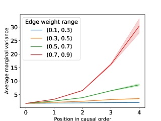
G.4 Varsortability Algorithm

The implementation is also available at https://github.com/Scriddie/Varsortability.

⬇

import numpy as np

def varsortability(X, W, tol=1e-9):

"""␣Takes␣n␣x␣d␣data␣and␣a␣d␣x␣d␣adjaceny␣matrix,

␣␣␣␣where␣the␣i,j-th␣entry␣corresponds␣to␣the␣edge␣weight␣for␣i->j,

␣␣␣␣and␣returns␣a␣value␣indicating␣how␣well␣the␣variance␣order

␣␣␣␣reflects␣the␣causal␣order.␣"""

E = W != 0

Ek = E.copy()

var = np.var(X, axis=0, keepdims=True)

n_paths = 0

n_correctly_ordered_paths = 0

for _ in range(E.shape[0] - 1):

n_paths += Ek.sum()

n_correctly_ordered_paths += (Ek * var / var.T > 1 + tol).sum()

n_correctly_ordered_paths += 1/2*(

(Ek * var / var.T <= 1 + tol) *

(Ek * var / var.T > 1 - tol)).sum()

Ek = Ek.dot(E)

return n_correctly_ordered_paths / n_paths

if __name__ == "__main__":

W = np.array([[0, 1, 0], [0, 0, 2], [0, 0, 0]])

X = np.random.randn(1000, 3).dot(np.linalg.inv(np.eye(3) - W))

print("Varsortability:", varsortability(X, W))

X_std = (X - np.mean(X, axis=0))/np.std(X, axis=0)

print("Varsortability␣standardized:", varsortability(X_std, W))

Appendix H sortnregress: A Diagnostic Tool to Reveal Varsortability

In Section 3.5 we introduce sortnregress as a simple baseline method. In the following subsections, we provide Python code that implements sortnregress thereby establishing its ease and illustrate how its DAG recovery performance reflects varying degrees of varsortability.

H.1 Implementation of Sortnregress

The implementation is also available at https://github.com/Scriddie/Varsortability.

⬇

import numpy as np

from sklearn.linear_model import LinearRegression, LassoLarsIC

def sortnregress(X):

"""␣Take␣n␣x␣d␣data,␣order␣nodes␣by␣marginal␣variance␣and

␣␣␣␣regresses␣each␣node␣onto␣those␣with␣lower␣variance,␣using

␣␣␣␣edge␣coefficients␣as␣structure␣estimates.␣"""

LR = LinearRegression()

LL = LassoLarsIC(criterion=’bic’)

d = X.shape[1]

W = np.zeros((d, d))

increasing = np.argsort(np.var(X, axis=0))

for k in range(1, d):

covariates = increasing[:k]

target = increasing[k]

LR.fit(X[:, covariates], X[:, target].ravel())

weight = np.abs(LR.coef_)

LL.fit(X[:, covariates] * weight, X[:, target].ravel())

W[covariates, target] = LL.coef_ * weight

return W

H.2 Varsortabiltiy and Score Attainable by Variance Ordering

In Figure 3 we observe that sortnregress improves linearly with varsortability. For a varsortability of 0.93 as in our experimental settings (cf. Section 3.3), it recovers the structure near-perfectly. randomregress uses a random ordering but is otherwise identical to sortnregress. The different ranges of varsortability can be classified as follows (n=30):

• < 0.33: sortnregress performs significantly worse than randomregress (p<1e-4)

• 0.33–0.66: no significant difference between sortnregress and randomregress (p=0.40)

• > 0.66: sortnregress performs significantly better than randomregress (p<1e-4)

Figure 3: Relationship between varsortability and score attainable through ordering by variance. Results shown for 10 simulated 10-node ER-1 graphs in each of 10 equally spaced varsortability bins. Note that for standard simulation settings most models have high varsortability. We use edge weights in $(-0.5,-0.1)\cup(0.1,0.5)$, Gumbel noise with standard deviations in $(0.5,2)$, and still need to discard many models with high varsortability to obtain $10$ instances per varsortability bin.

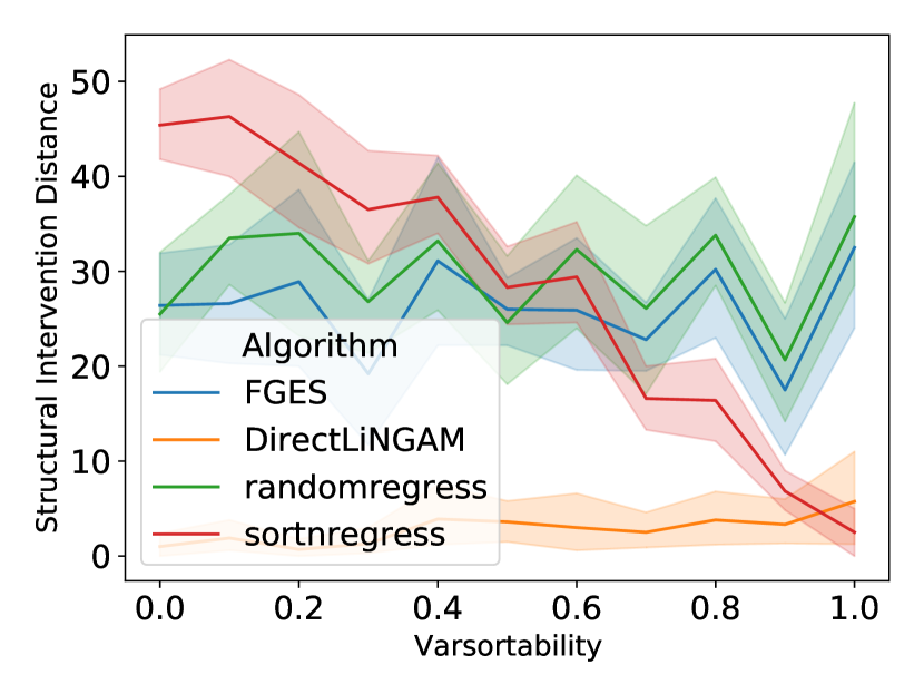
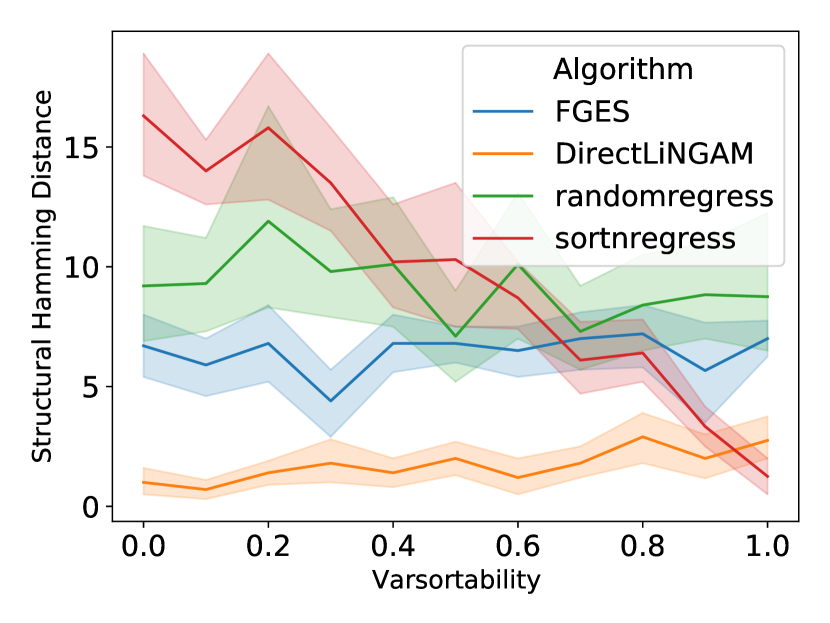
Appendix I Evaluation on Real-World Data

We analyze a dataset on protein signaling networks obtained by Sachs et al. [2005]. We evaluate our algorithms on ten bootstrap samples of the observational part of the dataset consisting of 853 observations, 11 nodes, and 17 edges. Our results show that there is no dominating algorithm. On average, most algorithms achieve performances similar to those of randomregress or the empty graph. Note that the results in terms of SHD are susceptible to thresholding choices and the empty graph baseline outperforms a majority of the algorithms. Our results are in line with previous reports [Lachapelle et al., 2019, Ng et al., 2020]. We observe scale-sensitivity of the continuous learning algorithms and sortnregress. However, in contrast to our simulation study in Section 4, the effect is small and inconsistent. The results do not show the patterns observed under high varsortability, which is consistent with the measured mean varsortability of $0.57$ with a standard deviation of $0.01$ across our bootstrapped samples.

Figure 4: SID (left) and SHD (right) performance of combinatorial and continuous methods on real-world data.

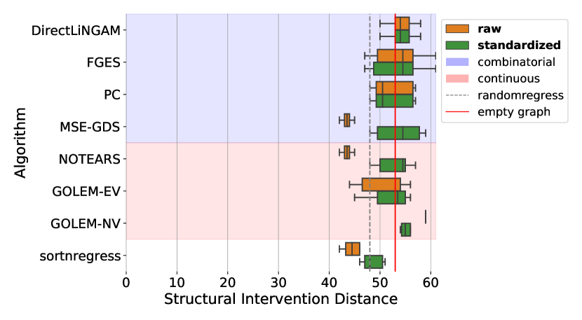
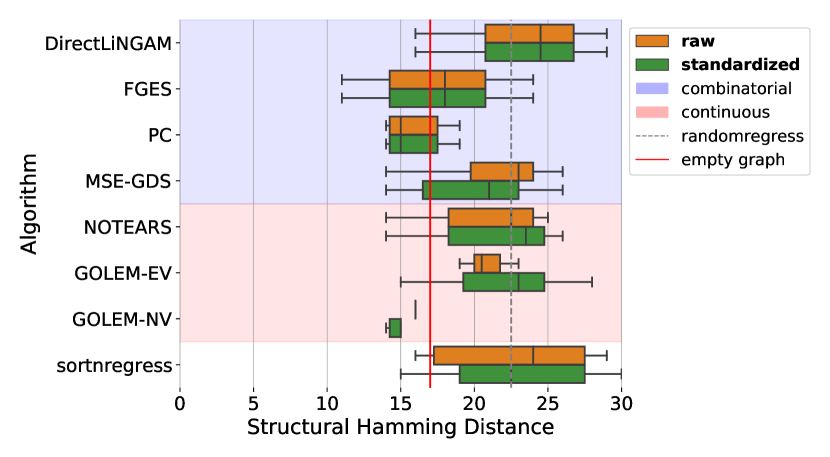
Appendix J Model Selection in Continuous Optimization

We illustrate the optimization landscape for the Gaussian MLE under Gaussian noise. This corresponds to the loss of GOLEM-NV as stated in Appendix D with a sparsity penalty of zero. We compare vanilla MLE to MLE with Lasso regularization for raw and standardized data. In Figure 5 we show the loss landscape in terms of SID and SHD difference to the true structure and highlight global optima. In the case of tied scores between the true structure and an alternative structure we select the true structure. For MLE with Lasso regularization using a penalty of $0.1$, the optimal loss is achieved by the true structure more frequently under standardization (red dots accumulate in the bottom left corner). Our result indicates that the Lasso sparsity penalty is influenced by the data scale and is better calibrated on standardized data. It is not unexpected that penalization is scale dependent, a problem that is, for example, discussed in applications of Ridge regression.

Figure 5: Standardized loss landscape for all 25 candidate graphs relative to each of the 25 possible 3-node ground-truth structures (a total of $25\times 25$ candidate-true graph pairs). The loss is scaled to $[0,1]$, see colorbar.

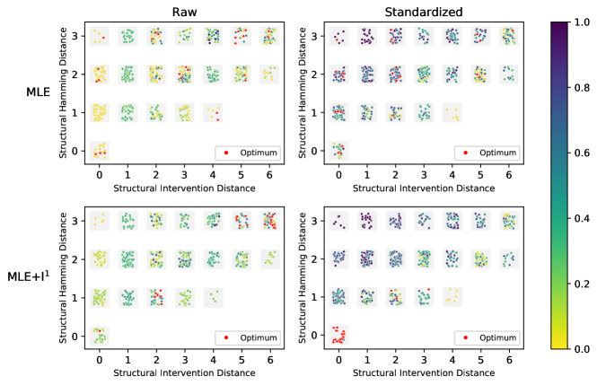
Appendix K Detailed Results

We provide a comprehensive overview over our empirical DAG/MEC recovery results for different evaluation metrics, graph types, and graph sizes.

K.1 MEC Recovery

An analysis of MEC recovery allows us to distinguish whether any drops in performance are within the expectations of identifiability. We evaluate the discovery of the MEC of the ground-truth DAG in a Gaussian setting with non-equal noise variances where only the ground-truth MEC but not the ground-truth DAG are identifiable. Since evaluating the SID between Markov equivalence classes is computationally expensive and prohibitively so for large graphs, we restrict ourselves to the setting here. When comparing MEC, we choose the upper limit of SID differences in Figure 1 in the main text. In Figure 6 we show that the relative performances are similar for the lower SID limit.

Figure 6: Lower bound of SID in MEC recovery for 10 node ER-2 graphs with non-equal Gaussian noise.

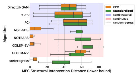
We conclude that the drop in performance extends from the recovery of the DAG to the recovery of the MEC and therefore goes beyond the difficulty of identifying the correct DAG within a MEC.

K.2 Results Across Thresholding Regimes

To ensure the effects we observe constitute a general phenomenon, we evaluate algorithm performance for different thresholding regimes. This is especially critical on standardized data. By re-scaling the data, standardization may impact the correct edge weights between nodes, potentially pushing them outside the thresholding range. Following Zheng et al. [2018], Ng et al. [2020], we perform thresholding for the continuous structure learning algorithms and prune edges with an edge weight in the recovered adjacency matrix of less than $0.3$. If the returned graph is not acyclic, we iteratively remove the edge with the smallest magnitude weight until all cycles are broken. We find that the qualitative performance differences between raw and standardized data are robust to a wide range of threshold choices.

Figure 7(a) and Figure 7(b) show SID performance for different thresholds. Even though the thresholds are orders of magnitude apart, a comparison reveals that the relative performances are nearly identical.

We observe that SHD performance is also robust across different thresholding regimes. Figure 7(c) shows performance using favorable thresholding. In this regime, the threshold leading to the most favorable SHD performance is applied to each instance individually. Figure 7(d) shows performance for a fixed threshold of 0.3. A comparison reveals nearly identical relative performances in both cases.

Overall, we observe that the effect of varsortability is present even for the most favorable threshold in case of SHD, and for a wide range of thresholds in case of SID, where computation of a favorable threshold is computationally infeasible.

(a) SID, threshold=0.001

(b) SID, threshold=0.3

(c) SHD, favorable thresholding

(d) SHD, threshold=0.3

Figure 7: Results for different thresholding regimes. Gaussian-NV noise, ER-2 graph, 50 nodes.

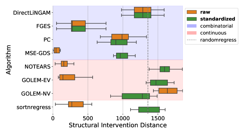
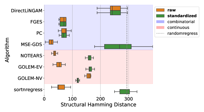
K.3 Results Across Noise Distributions and Graph Types

Figure 8 and Figure 9 show algorithm comparisons in terms of SID and SHD, respectively. The differences in performance on raw versus standardized data are qualitatively similar regardless of the noise distribution. We showcase results for different graph types in the non-Gaussian setting. DirectLiNGAM performs well only in the non-Gaussian cases, as is expected based on its underlying identifiability assumptions.

(a) SID, Gaussian-NV noise, ER-2 graph, 50 nodes

(b) SID, Gaussian-EV noise, ER-2 graph, 50 nodes

(c) SID, Exponential noise, ER-4 graph, 50 nodes

(d) SID, Gumbel noise, SF-4 graph, 50 nodes

Figure 8: SID results across noise types and for different graph types with 50 nodes

(a) SHD, Gaussian-NV noise, ER-2, 50 nodes

(b) SHD, Gaussian-EV noise, ER-2, 50 nodes

(c) SHD, Exponential Noise, ER-4, 50 nodes

(d) SHD, Gumbel Noise, SF-4, 50 nodes

Figure 9: SHD results across noise types and for different graph types with 50 nodes

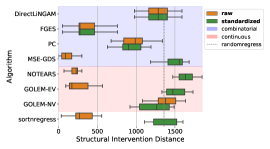
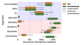
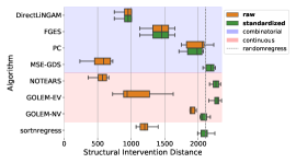
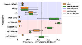
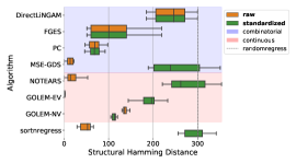
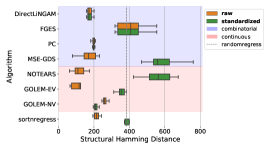
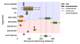
K.4 Results Across Noise Distributions, Graph Types, and Graph Sizes

The following experimental results largely follow earlier settings and results by Zheng et al. [2018], Ng et al. [2020].

(a) Raw data

(b) Standardized data

Figure 10: SID results across noise types, graph types, and graph sizes.

(a) Raw data

(b) Standardized data

Figure 11: SHD results across noise types, graph types, and graph sizes.

References

- Aragam and Zhou [2015] Bryon Aragam and Qing Zhou. Concave penalized estimation of sparse Gaussian Bayesian networks. Journal of Machine Learning Research, 16(69):2273–2328, 2015.
- Barabási and Albert [1999] Albert-László Barabási and Réka Albert. Emergence of scaling in random networks. Science, 286(5439):509–512, 1999.
- Bhattacharya et al. [2021] Rohit Bhattacharya, Tushar Nagarajan, Daniel Malinsky, and Ilya Shpitser. Differentiable causal discovery under unmeasured confounding. In International Conference on Artificial Intelligence and Statistics, 2021.
- Brouillard et al. [2020] Philippe Brouillard, Sébastien Lachapelle, Alexandre Lacoste, Simon Lacoste-Julien, and Alexandre Drouin. Differentiable causal discovery from interventional data. In Advances in Neural Information Processing Systems, 2020.
- Bühlmann et al. [2014] Peter Bühlmann, Jonas Peters, and Jan Ernest. CAM: Causal additive models, high-dimensional order search and penalized regression. The Annals of Statistics, 42(6):2526–2556, 2014.
- Chen et al. [2019] Wenyu Chen, Mathias Drton, and Y Samuel Wang. On causal discovery with an equal-variance assumption. Biometrika, 106(4):973–980, 09 2019.
- Chickering [1995] David M. Chickering. A Transformational Characterization of Equivalent Bayesian Network Structures. In Proceedings of the Eleventh Conference on Uncertainty in Artificial Intelligence (UAI), 1995.
- Chickering [1996] David M. Chickering. Learning Bayesian Networks is NP-complete. In Learning From Data, pages 121–130. Springer, 1996.
- Chickering [2002a] David M. Chickering. Learning equivalence classes of Bayesian-network structures. Journal of Machine Learning Research, 2:445–498, 2002a.
- Chickering [2002b] David M. Chickering. Optimal structure identification with greedy search. Journal of Machine Learning Research, 3(11):507–554, 2002b.
- Chickering et al. [2004] David M. Chickering, David Heckerman, and Chris Meek. Large-sample learning of Bayesian networks is NP-hard. Journal of Machine Learning Research, 5:1287–1330, 2004.
- Dawid [2010] A. Philip Dawid. Beware of the DAG! In Proceedings of Workshop on Causality: Objectives and Assessment at NIPS 2008, volume 6 of Proceedings of Machine Learning Research, pages 59–86. PMLR, 2010.
- Erdős and Rényi [1960] Paul Erdős and Alfréd Rényi. On the evolution of random graphs. Publication of the Mathematical Institute of the Hungarian Academy of Sciences, 5(1):17–60, 1960.
- Gao et al. [2020] Ming Gao, Yi Ding, and Bryon Aragam. A polynomial-time algorithm for learning nonparametric causal graphs. In Advances in Neural Information Processing Systems, 2020.
- Ghoshal and Honorio [2017] Asish Ghoshal and Jean Honorio. Learning Identifiable Gaussian Bayesian Networks in Polynomial Time and Sample Complexity. In Advances in Neural Information Processing Systems, 2017.
- Ghoshal and Honorio [2018] Asish Ghoshal and Jean Honorio. Learning linear structural equation models in polynomial time and sample complexity. In International Conference on Artificial Intelligence and Statistics, 2018.
- Hoyer et al. [2009] Patrik Hoyer, Dominik Janzing, Joris M. Mooij, Jonas Peters, and Bernhard Schölkopf. Nonlinear causal discovery with additive noise models. In Advances in Neural Information Processing Systems, 2009.
- Imbens and Rubin [2015] Guido W. Imbens and Donald B. Rubin. Causal inference in statistics, social, and biomedical sciences. Cambridge University Press, 2015.
- Kaiser and Sipos [2021] Marcus Kaiser and Maksim Sipos. Unsuitability of NOTEARS for Causal Graph Discovery. arXiv preprint arXiv:2104.05441, 2021.
- Lachapelle et al. [2019] Sébastien Lachapelle, Philippe Brouillard, Tristan Deleu, and Simon Lacoste-Julien. Gradient-based neural DAG learning. arXiv preprint arXiv:1906.02226, 2019.
- Lee et al. [2019] Hao-Chih Lee, Matteo Danieletto, Riccardo Miotto, Sarah T. Cherng, and Joel T. Dudley. Scaling structural learning with NO-BEARS to infer causal transcriptome networks. arXiv preprint arXiv:1911.00081, 2019.
- Loh and Bühlmann [2014] Po-Ling Loh and Peter Bühlmann. High-dimensional learning of linear causal networks via inverse covariance estimation. Journal of Machine Learning Research, 15:3065–3105, 2014.
- Meek [1995] Christopher Meek. Strong Completeness And Faithfulness In Bayesian Networks. In Proceedings of Eleventh Conference on Uncertainty in Artificial Intelligence (UAI), 1995.
- Meek [1997] Christopher Meek. Graphical Models: Selecting causal and statistical models. PhD thesis, Carnegie Mellon University, 1997.
- Mooij et al. [2020] Joris M. Mooij, Sara Magliacane, and Tom Claassen. Joint Causal Inference from Multiple Contexts. Journal of Machine Learning Research, 21(99):1–108, 2020.
- Ng et al. [2020] Ignavier Ng, AmirEmad Ghassami, and Kun Zhang. On the role of sparsity and DAG constraints for learning linear DAGs. In Advances in Neural Information Processing Systems, 2020.
- Pamfil et al. [2020] Roxana Pamfil, Nisara Sriwattanaworachai, Shaan Desai, Philip Pilgerstorfer, Konstantinos Georgatzis, Paul Beaumont, and Bryon Aragam. DYNOTEARS: Structure Learning from Time-Series Data. In International Conference on Artificial Intelligence and Statistics, 2020.
- Park [2020] Gunwoong Park. Identifiability of additive noise models using conditional variances. Journal of Machine Learning Research, 21(75):1–34, 2020.
- Pearl [2009] Judea Pearl. Causal inference in statistics: An overview. Statistics surveys, 3:96–146, 2009.
- Peters and Bühlmann [2014] Jonas Peters and Peter Bühlmann. Identifiability of Gaussian structural equation models with equal error variances. Biometrika, 101(1):219–228, 2014.
- Peters and Bühlmann [2015] Jonas Peters and Peter Bühlmann. Structural intervention distance for evaluating causal graphs. Neural Computation, 27(3):771–799, 2015.
- Peters et al. [2017] Jonas Peters, Dominik Janzing, and Bernhard Schölkopf. Elements of Causal Inference. MIT Press, 2017.
- Ramsey et al. [2018] Joseph D. Ramsey, Kun Zhang, Madelyn Glymour, Ruben S. Romero, Biwei Huang, Imme Ebert-Uphoff, Savini Samarasinghe, Elizabeth A. Barnes, and Clark Glymour. TETRAD—A toolbox for causal discovery. In 8th International Workshop on Climate Informatics (CI 2018), 2018.
- Rothman et al. [2008] Kenneth J. Rothman, Sander Greenland, and Timothy L. Lash. Modern Epidemiology. Lippincott Williams & Wilkins, 2008.
- Runge et al. [2020] Jakob Runge, Xavier-Andoni Tibau, Matthias Bruhns, Jordi Muñoz-Marí, and Gustau Camps-Valls. The causality for climate competition. In NeurIPS 2019 Competition and Demonstration Track, pages 110–120. PMLR, 2020.
- Sachs et al. [2005] Karen Sachs, Omar Perez, Dana Pe’er, Douglas A. Lauffenburger, and Garry P. Nolan. Causal protein-signaling networks derived from multiparameter single-cell data. Science, 308(5721):523–529, 2005.
- Sanford and Moosa [2012] Andrew D. Sanford and Imad A. Moosa. A Bayesian network structure for operational risk modelling in structured finance operations. Journal of the Operational Research Society, 63(4):431–444, 2012.
- Schölkopf [2019] Bernhard Schölkopf. Causality for machine learning. arXiv preprint arXiv:1911.10500, 2019.
- Schwarz [1978] Gideon Schwarz. Estimating the dimension of a model. The Annals of Statistics, 6(2):461–464, 1978.
- Shimizu et al. [2006] Shohei Shimizu, Patrik O. Hoyer, Aapo Hyvärinen, and Antti Kerminen. A linear non-Gaussian acyclic model for causal discovery. Journal of Machine Learning Research, 7:2003–2030, 2006.
- Shimizu et al. [2011] Shohei Shimizu, Takanori Inazumi, Yasuhiro Sogawa, Aapo Hyvärinen, Yoshinobu Kawahara, Takashi Washio, Patrik O. Hoyer, and Kenneth Bollen. DirectLiNGAM: A direct method for learning a linear non-Gaussian structural equation model. Journal of Machine Learning Research, 12:1225–1248, 2011.
- Shojaie and Michailidis [2010] Ali Shojaie and George Michailidis. Penalized likelihood methods for estimation of sparse high-dimensional directed acyclic graphs. Biometrika, 97(3):519–538, 07 2010.
- Spirtes and Glymour [1991] Peter Spirtes and Clark Glymour. An algorithm for fast recovery of sparse causal graphs. Social Science Computer Review, 9(1):62–72, 1991.
- Spirtes et al. [2000] Peter Spirtes, Clark N. Glymour, Richard Scheines, and David Heckerman. Causation, Prediction, and Search. MIT press, 2000.
- Tibshirani [1996] Robert Tibshirani. Regression shrinkage and selection via the lasso. Journal of the Royal Statistical Society: Series B (Methodological), 58(1):267–288, 1996.
- Vowels et al. [2021] Matthew J. Vowels, Necati Cihan Camgoz, and Richard Bowden. D’ya like DAGs? A Survey on Structure Learning and Causal Discovery. arXiv preprint arXiv:2103.02582, 2021.
- Wei et al. [2020] Dennis Wei, Tian Gao, and Yue Yu. DAGs with No Fears: A Closer Look at Continuous Optimization for Learning Bayesian Networks. arXiv preprint arXiv:2010.09133, 2020.
- Weichwald et al. [2020] Sebastian Weichwald, Martin E. Jakobsen, Phillip B. Mogensen, Lasse Petersen, Nikolaj Thams, and Gherardo Varando. Causal structure learning from time series: Large regression coefficients may predict causal links better in practice than small p-values. In NeurIPS 2019 Competition and Demonstration Track, pages 27–36. PMLR, 2020.
- Yang and Chang [2002] Shulin Yang and Kuo-Chu Chang. Comparison of score metrics for Bayesian network learning. IEEE Transactions on Systems, Man, and Cybernetics-Part A: Systems and Humans, 32(3):419–428, 2002.
- Yu et al. [2019] Yue Yu, Jie Chen, Tian Gao, and Mo Yu. DAG-GNN: DAG structure learning with graph neural networks. arXiv preprint arXiv:1904.10098, 2019.
- Zhang and Spirtes [2008] Jiji Zhang and Peter Spirtes. Detection of unfaithfulness and robust causal inference. Minds and Machines, 18(2):239–271, 2008.
- Zhang and Hyvarinen [2009] Kun Zhang and Aapo Hyvarinen. On the identifiability of the post-nonlinear causal model. In Proceedings of the Twenty-Fifth Conference on Uncertainty in Artificial Intelligence (UAI), 2009.
- Zheng et al. [2018] Xun Zheng, Bryon Aragam, Pradeep K. Ravikumar, and Eric P. Xing. DAGs with NO TEARS: Continuous optimization for structure learning. In Advances in Neural Information Processing Systems, 2018.
- Zheng et al. [2020] Xun Zheng, Chen Dan, Bryon Aragam, Pradeep K. Ravikumar, and Eric P. Xing. Learning sparse nonparametric DAGs. In International Conference on Artificial Intelligence and Statistics, 2020.