Abstract

We present a flexible trust region descend algorithm for unconstrained and convexly constrained multiobjective optimization problems. It is targeted at heterogeneous and expensive problems, i.e., problems that have at least one objective function that is computationally expensive. The method is derivative-free in the sense that neither need derivative information be available for the expensive objectives nor are gradients approximated using repeated function evaluations as is the case in finite-difference methods. Instead, a multiobjective trust region approach is used that works similarly to its well-known scalar pendants. Local surrogate models constructed from evaluation data of the true objective functions are employed to compute possible descent directions. In contrast to existing multiobjective trust region algorithms, these surrogates are not polynomial but carefully constructed radial basis function networks. This has the important advantage that the number of data points scales linearly with the parameter space dimension. The local models qualify as fully linear and the corresponding general scalar framework is adapted for problems with multiple objectives. Convergence to Pareto critical points is proven and numerical examples illustrate our findings.

1 1 0 https://doi.org/ Derivative-Free Multiobjective Trust Region Descent Method Using Radial Basis Function Surrogate Models Derivative-Free Multiobjective Trust Region Descent Method Using Radial Basis Function Surrogate Models Manuel Berkemeier ¹ and Sebastian Peitz ² Manuel Berkemeier and Sebastian Peitz Berkemeier, M.; Peitz, S. Correspondence: manuelbb@math.upb.de

1 Introduction

Optimization problems arise in a multitude of applications in mathematics, computer science, engineering and the natural sciences. In many real-life scenarios, there are multiple, equally important objectives that need to be optimized. Such problems are then called Multiobjective Optimization Problems (MOP). In contrast to the single objective case, an MOP often does not have a single solution but an entire set of optimal trade-offs between the different objectives, which we call Pareto optimal. They constitute the Pareto Set and their image is the Pareto Frontier. The goal in the numerical treatment of an MOP is to either approximate these sets or to find single points within these sets. In applications, the problem can become more difficult when some of the objectives require computationally expensive or time consuming evaluations. For instance, the objectives could depend on a computer simulation or some other black-box. It is then of primary interest to reduce the overall number of function evaluations. Consequently, it becomes infeasible to approximate derivative information of the true objectives using, e.g., finite differences. In this work, optimization methods that do not use the objective gradients (which nonetheless are assumed to exist) are referred to as derivative-free.

There is a variety of methods to deal with multiobjective optimization problems, some of which are also derivative-free or try to constrain the number of expensive function evaluations. A broad overview of different problems and techniques concerning multiobjective optimization can be found, e.g., in Ehrgott (2005); Jahn ; Miettinen (2013); Eichfelder (2020). One popular approach for calculating Pareto optimal solutions is scalarization, i.e., the transformation of an MOP into a single objective problem, cf. Eichfelder for an overview. Alternatively, classical (single objective) descent algorithms can be adapted for the multiobjective case Fukuda and Drummond ; Fliege and Svaiter ; Graña Drummond and Svaiter (2005); Lucambio Pérez and Prudente (a, b); Gebken et al. (2019). What is more, the structure of the Pareto Set can be exploited to find multiple solutions Hillermeier (2001); Gebken et al. (2019). There are also methods for non-smooth problems Wilppu et al. (2014); Gebken and Peitz (2021) and multiobjective direct-search variants Custódio et al. (2011); Audet et al. (2008). Both scalarization and descent techniques may be included in Evolutionary Algorithms (EA) Deb (2001); Coello et al. (2007); Abraham et al. (2005); Zitzler , the most prominent of which probably is NSGA-II Deb et al. (2002). To address computationally expensive objectives or missing derivative information, there are algorithms that use surrogate models (see the surveys Peitz and Dellnitz (2018); Chugh et al. (2019); Deb et al. (2020)) or borrow from ideas from scalar trust region methods, e.g., Roy et al. (2019).

In single objective optimization, trust region methods are well suited for derivative-free optimization Conn et al. ; Larson et al. (2019). Our work is based on the recent development of multiobjective trust region methods:

• In Qu et al. , a trust region method using Newton steps for functions with positive definite Hessians on an open domain is proposed.

• In Villacorta et al. quadratic Taylor polynomials are used to compute the steepest descent direction which is used in a backtracking manner to find solutions for unconstrained problems.

• In Ryu and Kim (2014) polynomial regression models are used to solve an augmented MOP based on the scalarization in Audet et al. (2008). The algorithm is designed unconstrained bi-objective problems.

• In Thomann and Eichfelder , quadratic Lagrange polynomials are used and the Pascoletti-Serafini scalarization is employed for the descent step calculation.

Our contribution is the extension of the above-mentioned methods to general fully linear models (and in particular radial basis function surrogates as in Wild et al. ), which is related to the scalar framework in Conn et al. (a). Most importantly, this reduces the complexity with respect to the parameter space dimension to linear, in contrast to the quadratically increasing number of function evaluations in other methods. We further prove convergence to critical points when the problem is constrained to a convex and compact set by using an analogous argumentation as in Conn et al. (b). This requires new results concerning the continuity of the projected steepest descent direction. We also show how to keep the convergence properties for constrained problems when the Pascoletti-Serafini scalarization is employed (like in Thomann and Eichfelder ).

The remainder of the paper is structured as follows: Section 2 provides a brief introduction to multiobjective optimality and criticality concepts. In Section 3 the fundamentals of our algorithm are explained. In Section 4 we introduce fully linear surrogate models and describe their construction. We also formalize the main algorithm in this section. Section 5 deals with the descent step calculation so that a sufficient decrease is achieved in each iteration. Convergence is proven in Section 6 and a few numerical examples are shown in Section 7. We conclude with a brief discussion in Section 8.

2 Optimality and Criticality in Multiobjective Optimization

We consider the following (real-valued) multiobjective optimization problem:

$$\min_{\bm{\mathrm{x}}\in\mathcal{X}}\bm{\mathrm{f}}(\bm{\mathrm{x}}):=\min_{\bm{\mathrm{x}}\in\mathcal{X}}\begin{bmatrix}f_{1}(\bm{\mathrm{x}})\\ \vdots\\ f_{k}(\bm{\mathrm{x}})\\ \end{bmatrix}\in\mathbb{R}^{k},$$ (MOP)

with a feasible set $\mathcal{X}\subseteq\mathbb{R}^{n}$ and $k$ objective functions $f_{\ell}\colon\mathbb{R}^{n}\to\mathbb{R},\ \ell=1,\ldots,k$. We further assume (MOP) to be heterogeneous. That is, there is a non-empty subset $I_{\text{ex}}\subseteq\{1,\ldots,k\}$ of indices so that the gradients of $f_{\ell},\ell\in I_{\text{ex}},$ are unknown and cannot be approximated, e.g., via finite differences. The (possibly empty) index set $I_{\text{cheap}}=\{1,\ldots,k\}\setminus I_{\text{ex}}$ indicates functions whose gradients are available.

Solutions for (MOP) consist of optimal trade-offs $\bm{\mathrm{x}}^{*}\in\mathcal{X}$ between the different objectives and are called non-dominated or Pareto optimal. That is, there is no $\bm{\mathrm{x}}\in\mathcal{X}$ with $\bm{\mathrm{f}}(\bm{\mathrm{x}})\prec\bm{\mathrm{f}}(\bm{\mathrm{x}}^{*})$ (i.e., $\bm{\mathrm{f}}(\bm{\mathrm{x}})\leq\bm{\mathrm{f}}(\bm{\mathrm{x}}^{*})$ and $f_{\ell}(\bm{\mathrm{x}})<f_{\ell}(\bm{\mathrm{x}}^{*})$ for some index $\ell\in\{1,\ldots,k\}$). The subset $\mathcal{P}_{\mathrm{S}}\subseteq\mathcal{X}$ of non-dominated points is then called the Pareto Set and its image $\mathcal{P}_{\mathrm{F}}:=\bm{\mathrm{f}}\left(\mathcal{P}_{\mathrm{S}}\right)\subseteq\mathbb{R}^{k}$ is called the Pareto Frontier. All concepts can be defined in a local fashion in an analogous way.

Similar to scalar optimization, local optima can be characterized using the gradients of the objective function. We therefore implicitly assume all objective functions $f_{\ell},\ell=1,\ldots,k,$ to be continuously differentiable on $\mathcal{X}$. Moreover, the following assumption allows for an easier treatment of tangent cones in the constrained case: Either $\mathcal{X}=\mathbb{R}^{n}$ or the feasible set $\mathcal{X}\subseteq\mathbb{R}^{n}$ is closed, bounded and convex. All functions are defined on $\mathcal{X}$.

Because $\mathbb{R}^{k}$ is finite-dimensional Section 2 is equivalent to requiring $\mathcal{X}$ to be compact and convex, which is a standard assumption in the MO literature Fliege and Svaiter ; Fukuda and Drummond .
Now let $\bm{\nabla}f_{\ell}(\bm{\mathrm{x}})$ denote the gradient of $f_{\ell}$ and ${\bm{\mathrm{D}}{\bm{\mathrm{f}}}}(\bm{\mathrm{x}})\in\mathbb{R}^{k\times n}$ the Jacobian of $\bm{\mathrm{f}}$ at $\bm{\mathrm{x}}\in\mathcal{X}$.

We call a vector $\bm{\mathrm{d}}\in\mathcal{X}-\bm{\mathrm{x}}$ a multi-descent direction for $\bm{\mathrm{f}}$ in $\bm{\mathrm{x}}$ if $\langle\bm{\nabla}f_{\ell}(\bm{\mathrm{x}}),\bm{\mathrm{d}}\rangle<0\quad$ for all $\ell\in\{1,\ldots,k\},$ or equivalently if

$$\max_{\ell=1,\ldots,k}\langle\bm{\nabla}f_{\ell}(\bm{\mathrm{x}}^{*}),\bm{\mathrm{d}}\rangle<0$$ (1)

where $\langle\bullet,\bullet\rangle$ is the standard inner product on $\mathbb{R}^{n}$ and we consider $\mathcal{X}-\bm{\mathrm{x}}=\mathcal{X}$ in the unconstrained case $\mathcal{X}=\mathbb{R}^{n}$.

A point $\bm{\mathrm{x}}^{*}\in\mathcal{X}$ is called critical for (MOP) iff there is no $\bm{\mathrm{d}}\in\mathcal{X}-\bm{\mathrm{x}}^{*}$ with (1). As all Pareto optimal points are also critical (cf. Fukuda and Drummond ; Luc or (Jahn, , Ch. 17)), it is viable to search for optimal points by calculating points from the superset $\mathcal{P}_{\mathrm{crit}}\supseteq\mathcal{P}_{\mathrm{S}}$ of critical points for (MOP). One way to do so is by iteratively performing descent steps. Fliege and Svaiter propose several ways to compute suitable descent directions. The minimizer $\bm{\mathrm{d}}^{*}$ of the following problem is known as the multiobjective steepest-descent direction.

$$\min_{\bm{\mathrm{d}}\in\mathcal{X}-\bm{\mathrm{x}}}\max_{\ell=1,\ldots,k}\langle\bm{\nabla}f_{\ell}(\bm{\mathrm{x}}),\bm{\mathrm{d}}\rangle\quad\text{s.t.}\quad\left\|\bm{\mathrm{d}}\right\|\leq 1.$$ (P1)

Problem (P1) has an equivalent reformulation as

$$\min_{\bm{\mathrm{d}}\in\mathcal{X}-\bm{\mathrm{x}}}\beta\qquad\text{s.t.}\quad\left\|\bm{\mathrm{d}}\right\|\leq 1\quad\mbox{and}\quad\langle\bm{\nabla}f_{\ell}(\bm{\mathrm{x}}),\bm{\mathrm{d}}\rangle\leq\beta\leavevmode\nobreak\ \forall\leavevmode\nobreak\ \ell=1,\ldots,k,$$ (P2)

which is a linear program, if $\mathcal{X}$ is defined by linear constraints and the maximum-norm $\left\|\bullet\right\|=\left\|\bullet\right\|_{\infty}$ is used Fliege and Svaiter . We thus stick with this choice because it facilitates implementation, but note that other choices are possible (see for example Thomann and Eichfelder ).

Motivated by the next theorem we can use the optimal value of either problem as a measure of criticality, i.e., as a multiobjective pendant for the gradient norm. As is standard in most multiobjective trust region works (cf. Qu et al. ; Villacorta et al. ; Thomann and Eichfelder ), we flip the sign so that the values are non-negative.

For $\bm{\mathrm{x}}\in\mathcal{X}$ let $\bm{\mathrm{d}}^{*}(\bm{\mathrm{x}})$ be the minimizer of (P1) and $\omega\left(\bm{\mathrm{x}}\right)$ be the negative optimal value, that is

$$\omega\left(\bm{\mathrm{x}}\right):=-\max_{\ell=1,\ldots,k}\langle\bm{\nabla}f_{\ell}(\bm{\mathrm{x}}),\bm{\mathrm{d}}^{*}(\bm{\mathrm{x}})\rangle.$$

Then the following statements hold:

1. $\omega\left(\bm{\mathrm{x}}\right)\geq 0$ for all $\bm{\mathrm{x}}\in\mathcal{X}$.

2. The function $\omega\colon\mathbb{R}^{n}\to\mathbb{R}$ is continuous.

3. The following statements are equivalent:

   1. The point $\bm{\mathrm{x}}\in\mathcal{X}$ is not critical.

   2. $\omega\left(\bm{\mathrm{x}}\right)>0$.

   3. $\bm{\mathrm{d}}^{*}(\bm{\mathrm{x}})\neq\bm{\mathrm{0}}$.

Consequently, the point $\bm{\mathrm{x}}$ is critical iff $\omega\left(\bm{\mathrm{x}}\right)=0$.

Proof.

For the unconstrained case all statements are proven in (Fliege and Svaiter, , Lemma 3).
The first and the third statement hold true for $\mathcal{X}$ convex and compact by definition. The continuity of $\omega$ can be shown similarly as in Fukuda and Drummond , see Section A.1. ∎

With further conditions on $\bm{\mathrm{f}}$ and $\mathcal{X}$ the criticality measure $\omega\left(\bm{\mathrm{x}}\right)$ is even Lipschitz continuous and subsequently uniformly and Cauchy continuous:

If $\bm{\nabla}f_{\ell},\ell=1,\ldots,k,$ are Lipschitz continuous and Section 2 holds, then the map $\omega\left(\bullet\right)$ as defined in Section 2 is uniformly continuous.

Proof.

The proof for $\mathcal{X}=\mathbb{R}^{n}$ is given by Thomann (2018). A proof for the constrained case can be found in Section A.1 as to not clutter this introductory section. ∎

Together with Section 2 this hints at $\omega\left(\bullet\right)$ being a criticality measure as defined for scalar trust region methods in (Conn et al., b, Ch. 8):

We call $\pi\colon\mathbb{N}_{0}\times\mathbb{R}^{n}\to\mathbb{R},$ a criticality measure for (MOP) if $\pi$ is Cauchy continuous with respect to its second argument and if

$$\lim_{t\to\infty}\pi(t,\bm{\mathrm{x}}^{(t)})=0$$

implies that the sequence $\left\{\bm{\mathrm{x}}^{(t)}\right\}$ asymptotically approaches a Pareto-critical point.

3 Trust Region Ideas

Multiobjective trust region algorithms closely follow the design of scalar approaches (see Conn et al. (b) for an extensive treatment). Consequently, the requirements and convergence proofs in Qu et al. ; Villacorta et al. ; Thomann and Eichfelder for the unconstrained multiobjective case are fairly similar to those in Conn et al. (b). We will reexamine the core concepts to provide a clear understanding and point out the similarities to the scalar case.

The main idea is to iteratively compute multi-descent steps $\bm{\mathrm{s}}^{(t)}$ in every iteration $t\in\mathbb{N}_{0}$. We could, for example, use the steepest descent direction given by (P1). This would require knowledge of the objective gradients - which need not be available for objective functions with indices in $I_{\text{ex}}$. Hence, benevolent surrogate model functions

$$\bm{\mathrm{m}}^{(t)}\colon\mathbb{R}^{n}\to\mathbb{R}^{k},\;\bm{\mathrm{x}}\mapsto\bm{\mathrm{m}}^{(t)}(\bm{\mathrm{x}})=\begin{bmatrix}m_{1}^{(t)}(\bm{\mathrm{x}}),\ldots,m_{k}^{(t)}(\bm{\mathrm{x}})\end{bmatrix}^{T},$$

are employed. Note, that for cheap objectives $f_{\ell},\ell\in I_{\text{cheap}},$ we could simply use $m_{\ell}=f_{\ell}$ as long as these $f_{\ell}$ are twice continuously differentiable and have Hessians of bounded norm.

The surrogate models are constructed to be sufficiently accurate within a trust region

$$B^{(t)}:=B\left(\bm{\mathrm{x}}^{(t)};\Delta^{(t)}\right)=\left\{\bm{\mathrm{x}}\in\mathcal{X}:\left\|\bm{\mathrm{x}}-\bm{\mathrm{x}}^{(t)}\right\|\leq\Delta^{(t)}\right\},\quad\text{with $\left\|\bullet\right\|=\left\|\bullet\right\|_{\infty}$,}$$ (2)

around the current iterate $\bm{\mathrm{x}}^{(t)}$. The model steepest descent direction $\bm{\mathrm{d}}^{(t)}_{\mathrm{m}}$ can then computed as the optimizer of the surrogate problem

$$\omega_{\mathrm{m}}^{(t)}\left(\bm{\mathrm{x}}^{(t)}\right):= -\min_{\bm{\mathrm{d}}\in\mathcal{X}-\bm{\mathrm{x}}}\beta$$ (Pm)

s.t. $$\left\|\bm{\mathrm{d}}\right\|\leq 1,\text{ and }\langle\bm{\nabla}m^{(t)}_{\ell}(\bm{\mathrm{x}}),\bm{\mathrm{d}}\rangle\leq\beta\quad\forall\ell=1,\ldots,k.$$

Now let $\sigma^{(t)}>0$ be a step size. The direction $\bm{\mathrm{d}}^{(t)}_{\mathrm{m}}$ need not be a descent direction for the true objectives $\bm{\mathrm{f}}$ and the trial point $\bm{\mathrm{x}}_{+}^{(t)}=\bm{\mathrm{x}}^{(t)}+\sigma^{(t)}\bm{\mathrm{d}}^{(t)}_{\mathrm{m}}$ is only accepted if a measure $\rho^{(t)}$ of improvement and model quality surpasses a positive threshold $\nu_{\scriptscriptstyle+}$. As in Villacorta et al. ; Thomann and Eichfelder , we scalarize the multiobjective problems by defining

$$\Phi(\bm{\mathrm{x}}):=\max_{\ell=1,\ldots,k}f_{\ell}(\bm{\mathrm{x}}),\qquad\Phi_{\mathrm{m}}^{(t)}(\bm{\mathrm{x}}):=\max_{\ell=1,\ldots,k}m_{\ell}^{(t)}(\bm{\mathrm{x}}).$$

Whenever $\Phi(\bm{\mathrm{x}}^{(t)})-\Phi(\bm{\mathrm{x}}_{+}^{(t)})>0$, there is a reduction in at least one objective function of $\bm{\mathrm{f}}$ because of

$$0<\Phi(\bm{\mathrm{x}}^{(t)})-\Phi(\bm{\mathrm{x}}_{+}^{(t)})=f_{\ell}(\bm{\mathrm{x}}^{(t)})-f_{q}(\bm{\mathrm{x}}_{+}^{(t)})\stackrel{{\scriptstyle\text{df.}}}{{\leq}}f_{\ell}(\bm{\mathrm{x}}^{(t)})-f_{\ell}(\bm{\mathrm{x}}_{+}^{(t)}),$$

where we denoted by $\ell$ the maximizing index in $\Phi(\bm{\mathrm{x}}^{(t)})$ and by $q$ the maximizing index in $\Phi(\bm{\mathrm{x}}_{+}^{(t)})$. Of course, the same property holds for $\Phi_{\mathrm{m}}^{(t)}(\bullet)$ and $\bm{\mathrm{m}}^{(t)}$.

Thus, the step size $\sigma^{(t)}>0$ is chosen so that the step $\bm{\mathrm{s}}^{(t)}=\sigma^{(t)}\bm{\mathrm{d}}^{(t)}_{\mathrm{m}}$ satisfies both $\bm{\mathrm{x}}^{(t)}+\bm{\mathrm{s}}^{(t)}\in B^{(t)}$ and a “sufficient decrease condition” of the form

$$\Phi_{\mathrm{m}}^{(t)}(\bm{\mathrm{x}}^{(t)})-\Phi_{\mathrm{m}}^{(t)}(\bm{\mathrm{x}}^{(t)}+\bm{\mathrm{s}}^{(t)})\geq\kappa^{\scriptstyle\mathrm{sd}}\omega\left(\bm{\mathrm{x}}^{(t)}\right)\min\left\{\mathrm{C}\cdot\omega\left(\bm{\mathrm{x}}^{(t)}\right),1,\Delta^{(t)}\right\}\geq 0,$$

with a constant $\mathrm{C}>0$, see Section 5. Such a condition is also required in the scalar case Conn et al. (b, a) and essential for the convergence proof in Section 6, where we show $\lim_{t\to\infty}\omega\left(\bm{\mathrm{x}}^{(t)}\right)=0$.

Due to the decrease condition the denominator in the ratio of actual versus predicted reduction,

$$\rho^{(t)}=\begin{dcases}\frac{\Phi(\bm{\mathrm{x}}^{(t)})-\Phi(\bm{\mathrm{x}}_{+}^{(t)})}{\Phi_{\mathrm{m}}^{(t)}(\bm{\mathrm{x}}^{(t)})-\Phi_{\mathrm{m}}^{(t)}(\bm{\mathrm{x}}_{+}^{(t)})}&\text{if $\bm{\mathrm{x}}^{(t)}\neq\bm{\mathrm{x}}_{+}^{(t)}$},\\ 0&\text{if $\bm{\mathrm{x}}^{(t)}=\bm{\mathrm{x}}_{+}^{(t)}\Leftrightarrow\bm{\mathrm{s}}^{(t)}=\bm{\mathrm{0}}$,}\end{dcases}$$ (3)

is nonnegative. A positive $\rho^{(t)}$ implies a decrease in at least one objective $f_{\ell}$, so we accept $\bm{\mathrm{x}}_{+}^{(t)}$ as the next iterate if $\rho^{(t)}>\nu_{\scriptscriptstyle+}>0$. If $\rho^{(t)}$ is sufficiently large, say $\rho^{(t)}\geq\nu_{{\scriptscriptstyle++}}>\nu_{\scriptscriptstyle+}>0$, the next trust region might have a larger radius $\Delta^{(t+1)}\geq\Delta^{(t)}$. If in contrast $\rho<\nu_{{\scriptscriptstyle++}}$, the next trust region radius should be smaller and the surrogates improved.
This encompasses the case $\bm{\mathrm{s}}^{(t)}=\bm{\mathrm{0}}$, when the iterate $\bm{\mathrm{x}}^{(t)}$ is critical for

$$\min_{\bm{\mathrm{x}}\in B^{(t)}}\bm{\mathrm{m}}^{(t)}(\bm{\mathrm{x}})\,\in\mathbb{R}^{k}. \mathrm{m}$$ (MOP)

Roughly speaking, we suppose that $\bm{\mathrm{x}}^{(t)}$ is near a critical point for the original problem (MOP) if $\bm{\mathrm{m}}^{(t)}$ is sufficiently accurate. If we truly are near a critical point, then the trust region radius will approach 0. For further details concerning the acceptance ratio $\rho^{(t)}$, see (Thomann and Eichfelder, , Sec. 2.2).

We can modify $\rho^{(t)}$ in (3) to obtain a descent in all objectives, i.e., if $\bm{\mathrm{x}}^{(t)}\neq\bm{\mathrm{x}}_{+}^{(t)}$ we test $\rho^{(t)}=\dfrac{f_{\ell}(\bm{\mathrm{x}}^{(t)})-f_{\ell}(\bm{\mathrm{x}}_{+}^{(t)})}{m^{(t)}_{\ell}(\bm{\mathrm{x}}^{(t)})-m^{(t)}_{\ell}(\bm{\mathrm{x}}_{+}^{(t)})}>\nu_{\scriptscriptstyle+}$ for all $\ell=1,\ldots,k$. This is the strict acceptance test.

4 Surrogate Models and the Final Algorithm

Until now, we have not discussed the actual choice of surrogate models used for $\bm{\mathrm{m}}^{(t)}$. As is shown in Section 5, the models should be twice continuously differentiable with uniformly bounded hessians. To prove convergence of our algorithm we have to impose further requirements on the (uniform) approximation qualities of the surrogates $\bm{\mathrm{m}}^{(t)}$. We can meet these requirements using so-called fully linear models. Moreover, fully linear models intrinsically allow for modifications of the basic trust region method that are aimed at reducing the total number of expensive objective evaluations. Finally, we briefly recapitulate how radial basis functions and multivariate Lagrange polynomials can be made fully linear.

4.1 Fully Linear Models

Let us begin with the abstract definition of full linearity as given in Conn et al. (a, ): Let ${\Delta}^{\mathrm{ub}}>0$ be given and let $f\colon\mathbb{R}\to\mathbb{R}$ be a function that is continuously differentiable in an open domain containing $\mathcal{X}$ and has a Lipschitz continuous gradient on $\mathcal{X}$. A set of model functions $\mathcal{M}=\left\{m\colon\mathbb{R}^{n}\to\mathbb{R}\right\}\subseteq C^{1}(\mathbb{R}^{n},\mathbb{R})$ is called a fully linear class of models if the following hold:

1. There are positive constants $\epsilon,\dot{\epsilon}$ and $L_{m}$ such that for any given $\Delta\in(0,{\Delta}^{\mathrm{ub}})$ and for any $\bm{\mathrm{x}}\in\mathcal{X}$ there is a model function $m\in\mathcal{M}$ with Lipschitz continuous gradient and corresponding Lipschitz constant bounded by $L_{m}$ and such that

   • the error between the gradient of the model and the gradient of the function satisfies

     $$\left\|\bm{\nabla}f(\bm{\upxi})-\bm{\nabla}m(\bm{\upxi})\right\|\leq\dot{\epsilon}\Delta,\quad\forall\bm{\upxi}\in B\left(\bm{\mathrm{x}};\Delta\right),$$

   • the error between the model and the function satisfies

     $$\left|f(\bm{\upxi})-m(\bm{\upxi})\right|\leq\epsilon\Delta^{2},\quad\forall\bm{\upxi}\in B\left(\bm{\mathrm{x}};\Delta\right).$$

2. For this class $\mathcal{M}$ there exists “model-improvement” algorithm that – in a finite, uniformly bounded (w.r.t. $\bm{\mathrm{x}}$ and $\Delta$) number of steps – can

   • either establish that a given model $m\in\mathcal{M}$ is fully linear on $B\left(\bm{\mathrm{x}};\Delta\right)$

   • or find a model $\tilde{m}$ that is fully linear on $B\left(\bm{\mathrm{x}};\Delta\right)$.

In the constrained case, we treat the constraints as hard, that is, we do not allow for evaluations of the true objectives outside $\mathcal{X}$, see the definition of $B^{(t)}\subseteq\mathcal{X}$ in (2). We also ensure to only select training data in $\mathcal{X}$ during the construction of surrogate models.

In the unconstrained case, the requirements in Section 4.1 can be relaxed a bit, at least when using the strict acceptance test with $\bm{\mathrm{f}}(\bm{\mathrm{x}}^{(T)})\leq\bm{\mathrm{f}}(\bm{\mathrm{x}}^{(t)})$ for all $T\geq t\geq 0$. We can then restrict ourselves to the set

$$\mathcal{X}^{\prime}:=\bigcup_{\bm{\mathrm{x}}\in L(\bm{\mathrm{x}}^{(0)})}B\left(\bm{\mathrm{x}};{\Delta}^{\mathrm{ub}}\right),\quad\text{where }L(\bm{\mathrm{x}}^{(0)}):=\left\{\bm{\mathrm{x}}\in\mathbb{R}^{n}:\bm{\mathrm{f}}(\bm{\mathrm{x}})\leq\bm{\mathrm{f}}(\bm{\mathrm{x}}^{(0)})\right\}.$$

For the convergence analysis in Section 6, we cite (Conn et al., , Lemma 10.25) concerning the approximation quality of fully linear models on enlarged trust regions: For $\bm{\mathrm{x}}\in\mathcal{X}$ and $\Delta\leq{\Delta}^{\mathrm{ub}}$ consider a function $f$ and a fully-linear model $m$ as in Section 4.1 with constants $\epsilon,\dot{\epsilon},L_{m}>0$. Let $L_{f}>0$ be a Lipschitz constant of $\bm{\nabla}f$.
Assume w.l.o.g. that

$$L_{m}+L_{f}\leq\epsilon\quad\text{and}\quad\frac{\dot{\epsilon}}{2}\leq\epsilon.$$

Then $m$ is fully linear on $B\left(\bm{\mathrm{x}};\tilde{\Delta}\right)$ for any $\tilde{\Delta}\in[\Delta,{\Delta}^{\mathrm{ub}}]$ with respect to the same constants $\epsilon,\dot{\epsilon},L_{m}$.

4.1.1 Algorithm Modifications

With Section 4.1 we have formalized our assumption that the surrogates become more accurate when we decrease the trust region radius. This motivates the following modifications:

• “Relaxing” the (finite) surrogate construction process to try for a possible descent even if the surrogates are not fully linear.

• A criticality test depending on $\varpi_{\mathrm{m}}^{(t)}\left(\bm{\mathrm{x}}^{(t)}\right)$. If this value is very small at the current iterate, then $\bm{\mathrm{x}}^{(t)}$ could lie near a Pareto-critical point. With the criticality test and criticalityRoutine we ensure that the next model is fully linear and the trust region is not too large. This allows for a more accurate criticality measure and descent step calculation.

• A trust region update that also takes into consideration $\varpi_{\mathrm{m}}^{(t)}\left(\bm{\mathrm{x}}^{(t)}\right)$. The radius should be enlarged if we have a large acceptance ratio $\rho^{(t)}$ and the $\Delta^{(t)}$ is small as measured against $\beta\omega_{\mathrm{m}}^{(t)}\left(\bm{\mathrm{x}}^{(t)}\right)$ for a constant $\beta>0$.

These changes are implemented in Algorithm 1. For more detailed explanations we refer to (Conn et al., , Ch. 10).

Configuration: Criticality parameters $\varepsilon_{\mathrm{crit}}>0$ and $\mu>\beta>0$, acceptance parameters $1>\nu_{{\scriptscriptstyle++}}\geq\nu_{\scriptscriptstyle+}\geq 0,\nu_{{\scriptscriptstyle++}}\neq 0$, update factors $\gamma_{\scriptscriptstyle\uparrow}\geq 1>\gamma_{\scriptscriptstyle\downarrow}\geq\gamma_{\scriptscriptstyle\downdownarrows}>0$ and ${\Delta}^{\mathrm{ub}}>0$;

Input: The initial site $\bm{\mathrm{x}}^{(0)}\in\mathbb{R}^{n}$;

for $t=0,1,\ldots$ do

       if $t>0$ and iteration $(t-1)$ was model-improving (cf. Section 4.1.1) then

             Perform at least one improvement step on $\bm{\mathrm{m}}^{(t-1)}$ and then let $\bm{\mathrm{m}}^{(t)}\leftarrow\bm{\mathrm{m}}^{(t-1)}$;

            

      else

             Construct surrogate models $\bm{\mathrm{m}}^{(t)}$ on $B^{(t)}$;

            

       end if

      /* Criticality Step: */

       if  $\varpi_{\mathrm{m}}^{(t)}\left(\bm{\mathrm{x}}^{(t)}\right)<\varepsilon_{\mathrm{crit}}$ and $\bigl{(}$ $\bm{\mathrm{m}}^{(t)}$ not fully linear or $\Delta^{(t)}>\mu\varpi_{\mathrm{m}}^{(t)}\left(\bm{\mathrm{x}}^{(t)}\right)$ $\bigr{)}$  then

             Set $\Delta^{(t)}_{*}\leftarrow\Delta^{(t)}$;

             Call $\text{{criticalityRoutine}}()$ so that $\bm{\mathrm{m}}^{(t)}$ is fully linear on $B^{(t)}$ with $\Delta^{(t)}\in(0,\mu\varpi_{\mathrm{m}}^{(t)}\left(\bm{\mathrm{x}}^{(t)}\right)]$;

             Then set $\Delta^{(t)}\leftarrow\min\left\{\max\left\{\Delta^{(t)},\beta\varpi_{\mathrm{m}}^{(t)}\left(\bm{\mathrm{x}}^{(t)}\right)\right\},\Delta^{(t)}_{*}\right\}$ ;

            

       end if

      Compute a suitable descent step $\bm{\mathrm{s}}^{(t)}$;

       Set $\bm{\mathrm{x}}_{+}^{(t)}\leftarrow\bm{\mathrm{x}}^{(t)}+\bm{\mathrm{s}}^{(t)}$, evaluate $\bm{\mathrm{f}}(\bm{\mathrm{x}}_{+}^{(t)})$ and compute $\rho^{(t)}$ with (3);

       Perform the following updates:

      

$$\bm{\mathrm{x}}^{(t+1)} \leftarrow\begin{cases}\bm{\mathrm{x}}^{(t)}&\text{if $\rho^{(t)}<\nu_{\scriptscriptstyle+}$},\\ \bm{\mathrm{x}}_{+}^{(t)}&\text{if $\nu_{\scriptscriptstyle+}\leq\rho^{(t)}<\nu_{{\scriptscriptstyle++}}$ \& $\bm{\mathrm{m}}^{(t)}$ is fully linear,}\\ \bm{\mathrm{x}}_{+}^{(t)}&\text{if $\nu_{{\scriptscriptstyle++}}\leq\rho^{(t)}$}.\end{cases}$$

$$\Delta^{(t+1)} \leftarrow\Delta_{+},\text{ where }$$

$$\Delta_{+} \begin{cases}=\Delta^{(t)}&\text{if $\rho^{(t)}<\nu_{{\scriptscriptstyle++}}$ \& $\bm{\mathrm{m}}^{(t)}$ is {not} fully linear},\\ \in[\gamma_{\scriptscriptstyle\downdownarrows}\Delta^{(t)},\gamma_{\scriptscriptstyle\downarrow}\Delta^{(t)}]&\text{if $\rho^{(t)}<\nu_{{\scriptscriptstyle++}}$ \& $\bm{\mathrm{m}}^{(t)}$ is fully linear},\\ \in\left[\Delta^{(t)},\min\{\gamma_{\scriptscriptstyle\uparrow}\Delta^{(t)},{\Delta}^{\mathrm{ub}}\}\right]&\text{if $\nu_{{\scriptscriptstyle++}}\leq\rho^{(t)}$ and $\Delta^{(t)}\geq\beta\omega_{\mathrm{m}}^{(t)}\left(\bm{\mathrm{x}}^{(t)}\right)$,}\\ =\min\{\gamma_{\scriptscriptstyle\uparrow}\Delta^{(t)},{\Delta}^{\mathrm{ub}}\}&\text{if $\nu_{{\scriptscriptstyle++}}\leq\rho^{(t)}$ and $\Delta^{(t)}<\beta\omega_{\mathrm{m}}^{(t)}\left(\bm{\mathrm{x}}^{(t)}\right)$.}\\ \end{cases}$$

      

end for

Algorithm 1 General TRM for (MOP)

[htb]    Configuration: backtracking constant $\alpha\in(0,1)$, $\mu>\beta>0$ from Algorithm 1; Set $\Delta_{0}\leftarrow\Delta^{(t)}$;

for  $j=1,2,\ldots$  do

       Set radius: $\Delta^{(t)}\leftarrow\alpha^{j-1}\Delta_{0}$;

       Make models $\bm{\mathrm{m}}^{(t)}$ fully linear on $B^{(t)}$ ;

        /* can change $\varpi_{\mathrm{m}}^{(t)}\left(\bm{\mathrm{x}}^{(t)}\right)$ */ if  $\Delta^{(t)}\leq\mu\varpi_{\mathrm{m}}^{(t)}\left(\bm{\mathrm{x}}^{(t)}\right)$  then

             Break;

            

       end if

      

end for

criticalityRoutine()  

From Algorithm 1 we see that we can classify the iterations based on $\rho^{(t)}$ in the following way: For given constants $0\leq\nu_{\scriptscriptstyle+}\leq\nu_{{\scriptscriptstyle++}}<1,\nu_{{\scriptscriptstyle++}}\neq 0,$ we call the iteration with index $t\in\mathbb{N}_{0}$ of Algorithm 1 …

• …successful if $\rho^{(t)}\geq\nu_{{\scriptscriptstyle++}}$. The set of successful indices is $\mathcal{S}=\{t\in\mathbb{N}_{0}:\rho^{(t)}\geq\nu_{{\scriptscriptstyle++}}\}\subseteq\mathbb{N}_{0}$.

• …model-improving if $\rho^{(t)}<\nu_{{\scriptscriptstyle++}}$ and the models $\bm{\mathrm{m}}^{(t)}=[m_{1}^{(t)},\ldots,m_{k}^{(t)}]^{T}$ are not fully linear. In these iterations the trust region radius is not changed.

• …acceptable if $\nu_{\scriptscriptstyle+}>\rho^{(t)}\geq\nu_{\scriptscriptstyle+}$ and the models $\bm{\mathrm{m}}^{(t)}$ are fully linear. If $\nu_{{\scriptscriptstyle++}}=\nu_{\scriptscriptstyle+}\in(0,1)$, then there are no acceptable indices.

• …inacceptable otherwise, i.e., if $\rho^{(t)}<\nu_{\scriptscriptstyle+}$ and $\bm{\mathrm{m}}^{(t)}$ are fully linear.

4.2 Fully Linear Lagrange Polynomials

Quadratic Taylor polynomial models are used very frequently. As explained in Conn et al. we can alternatively use multivariate interpolating Lagrange polynomial models when derivative information is not available. We will consider first and second degree Lagrange models. Even though the latter require $\mathcal{O}(n^{2})$ function evaluations they are still cheaper than second degree finite difference models. For this reason, these models are also used in Thomann and Eichfelder ; Thomann (2018).

To construct an interpolating polynomial model we have to provide $p$ data sites, where $p$ is the dimension of the space $\Pi_{n}^{d}$ of real-valued $n$-variate polynomials with degree $d$. For $d=1$ we have $p=n+1$ and for $d=2$ it is $p=\dfrac{(n+1)(n+2)}{2}$. If $n\geq 2$, the Mairhuber-Curtis theoremWendland (2004) applies and the data sites must form a so-called poised set in $\mathcal{X}$. The set $\Xi=\{\bm{\upxi}_{1},\ldots,\bm{\upxi}_{p}\}\subset\mathbb{R}^{n}$ is poised if for any basis $\{\psi_{i}\}$ of $\Pi_{n}^{d}$ the matrix $\bm{\mathrm{M}}_{\psi}:=\left[\psi_{i}(\bm{\upxi}_{j})\right]_{1\leq i,j\leq p}$ is non-singular. Then there is a unique polynomial $m(\bm{\mathrm{x}})=\sum_{i=1}^{p}\lambda_{i}\psi_{i}(\bm{\mathrm{x}})$ with $m(\bm{\upxi}_{j})=F(\bm{\upxi}_{j})$ for all $j=1,\ldots,p$ and any function $F\colon\mathbb{R}^{n}\to\mathbb{R}$. Given a poised set $\Xi$ the associated Lagrange basis $\{l_{i}\}$ of $\Pi_{n}^{d}$ is defined by $l_{i}(\bm{\mathrm{\upxi_{j}}})=\delta_{i,j}$. The model coefficients then simply are the data values, i.e., $\lambda_{i}=F(\bm{\upxi}_{i})$.

Same as in Thomann (2018), we implement Algorithm 6.2 from Conn et al. to ensure poisedness. It selects training sites $\Xi$ from the current (slightly enlarged) trust region of radius $\theta_{1}\Delta^{(t)}$ and calculates the associated lagrange basis. We can then separately evaluate the true objectives $f_{\ell}$ on $\Xi$ to easily build the surrogates $m_{\ell}^{(t)}$, $\ell\in\{1,\ldots,k\}$. Our implementation always includes $\bm{\upxi}_{1}=\bm{\mathrm{x}}^{(t)}$ and tries to select points from a database of prior evaluations first.

We employ an additional algorithm (Algorithm 6.3 in Conn et al. ) to ensure that the set $\Xi$ is even $\Lambda$-poised, see (Conn et al., , Definition 3.6). The procedure is still finite and ensures the models are actually fully linear. The quality of the surrogate models can be improved by choosing a small algorithm parameter $\Lambda>1$. Our implementation tries again to recycle points from a database. Different to before, interpolation at $\bm{\mathrm{x}}^{(t)}$ can no longer be guaranteed. This second step can also be omitted first and then used as a model-improvement step in a subsequent iteration.

4.3 Fully Linear Radial Basis Function Models

The main drawback of quadratic Lagrange models is that we still need $\mathcal{O}(n^{2})$ function evaluations in each iteration of Algorithm 1. A possible fix is to use under-determined regression polynomials instead Conn et al. ; Stefan (2008); Ryu and Kim (2014). Motivated by the findings in Wild et al. we chose so-called Radial Basis Function (RBF) models as an alternative. RBF are well-known for their approximation capabilities on irregular data Wendland (2004). In our implementation they have the form

$$m(\bm{\mathrm{x}})=\sum_{i=1}^{N}c_{i}\varphi\left(\left\|\bm{\mathrm{x}}-\bm{\upxi}_{i}\right\|_{2}\right)+\pi(\bm{\mathrm{x}}),\quad\pi=\sum_{i}\lambda_{i}\psi_{i}\in\Pi_{n}^{d},d\in\{0,1\},N\in\mathbb{N},$$ (4)

where $\varphi$ is a function from $\mathbb{R}_{\geq 0}$ to $\mathbb{R}$. For a fixed $\varphi$ the mapping $\varphi\left(\left\|\bullet\right\|\right)$ from $\mathbb{R}^{n}\to\mathbb{R}$ is radially symmetric with respect to its argument and the mapping $(\bm{\mathrm{x}},\bm{\upxi})\mapsto\varphi\left(\left\|\bm{\mathrm{x}}-\bm{\upxi}\right\|_{2}\right)$ is called a kernel.

Wild et al. describe a construction of RBF surrogate models as in (4) (see also Wild and Shoemaker and the dissertation Stefan (2008) for more details). If we restrict ourselves to functions $\varphi\left(\left\|\bullet\right\|\right)$ that are conditionally positive definite (c.p.d. – see Wendland (2004); Wild et al. for the definition) of order at most two, then the surrogates can be made certifiably fully linear with $N=n+1$. As before, the algorithms tries to select an initial training set $\Xi=\{\bm{\upxi}_{1},\ldots,\bm{\upxi}_{N}\}\subset B(\bm{\mathrm{x}}^{(t)};\theta_{1}\Delta^{(t)})$ with $N=n+1$ and a scaling factor $\theta_{1}\geq 1$. The set must be poised for interpolation with affine linear polynomials. Due to $\varphi\left(\left\|\bullet\right\|\right)$ being c.p.d. of order $D\leq 2$, the interpolation system

$$\begin{bmatrix}\bm{\Upphi}&\bm{\mathrm{M}}_{\psi}^{T}\\ \bm{\mathrm{M}}_{\psi}&\bm{\mathrm{0}}\end{bmatrix}\cdot\begin{bmatrix}\bm{\mathrm{c}}\\ \bm{\uplambda}\end{bmatrix}=\begin{bmatrix}\bm{\mathrm{F}}(\Xi)\\ \bm{\mathrm{0}}\end{bmatrix}\in\mathbb{R}^{N+p\times 1},$$

$$\bm{\mathrm{c}}=[c_{i}]_{1\leq i\leq N},\ \bm{\uplambda}=[\lambda_{i}]_{1\leq i\leq p},\ \bm{\Upphi}=[\varphi\left(\left\|\bm{\upxi}_{i}-\bm{\upxi}_{j}\right\|\right)]_{1\leq i,j\leq N},$$

is uniquely solvable for any $F\colon\mathbb{R}^{n}\to\mathbb{R}$ if we choose $\Pi_{n}^{d}$ such that $d\geq\max\{0,D-1\}$. We can even include more points, $N\geq n+1$, from within a region of maximum radius $\theta_{2}{\Delta}^{\mathrm{ub}}$, $\theta_{2}\geq\theta_{1}\geq 1$, to capture nonlinear behavior of $F$. More detailed explanations can be found in Wild et al. . Modifications for box constraints are shown in Stefan (2008) and Regis and Wild (2017).

[H] Some radial functions $\varphi\colon\mathbb{R}_{\geq 0}\to\mathbb{R}$ that are c.p.d. of order $D\leq 2$, cf. Wild et al. . Name $\varphi(r)$ c.p.d. order $D$ $\deg\pi$ Cubic $r^{3}$ $2$ $1$ Multiquadric $-\sqrt{1+(\alpha r)^{2}},\alpha>0$ $1$ $\{0,1\}$ Gaussian $\exp(-(\alpha r)^{2}),\alpha>0$ $0$ $\{0,1\}$

Section 4.3 shows the RBF we are using and the possible polynomial degrees for $\pi$. Both the Gaussian and the Multiquadric allow for fine-tuning with a shape parameter $\alpha>0$. This can potentially improve the conditioning of the interpolation system. Fig. 1 (b) illustrates the effect of the shape parameter. As can be seen, the radial functions become narrower for larger shape parameters. Hence, we do not only use a constant shape parameter $\alpha=1$ like Wild et al. do, but we also use an $\alpha$ that is (within lower and upper bounds) inversely proportional to $\Delta^{(t)}$.
Fig. 1 (a) shows interpolation of a nonlinear function by a surrogate based on the Multiquadric with a linear tail.

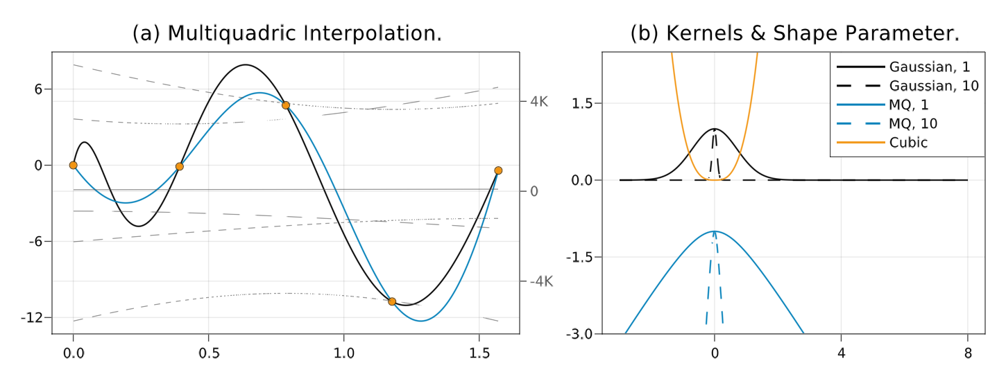
Figure 1: (a) Interpolation of a nonlinear function (black) by a Multiquadric surrogate (black) based on 5 discrete training points (orange). Dashed lines show the kernels and the polynomial tail. (b) Different kernels in 1D with varying shape parameter ($1$ or $10$), see also Section 4.3.

5 Descent Steps

In this section we introduce some possible steps $\bm{\mathrm{s}}^{(t)}$ to use in Algorithm 1. We begin by defining the best step along the steepest descent direction as given by (Pm). Subsequently, backtracking variants are defined that use a multiobjective variant of Armijo’s rule.

5.1 Pareto-Cauchy Step

Both the Pareto-Cauchy point as well as a backtracking variant, the modified Pareto-Cauchy point, are points along the descent direction $\bm{\mathrm{d}}^{(t)}_{\mathrm{m}}$ within $B^{(t)}$ so that a sufficient decrease measured by $\Phi_{\mathrm{m}}^{(t)}(\bullet)$ and $\omega_{\mathrm{m}}^{(t)}\left(\bullet\right)$ is achieved. Under mild assumptions we can then derive a decrease in terms of $\omega\left(\bullet\right)$.

For $t\in\mathbb{N}_{0}$ let $\bm{\mathrm{d}}^{(t)}_{\mathrm{m}}$ be a minimizer for (Pm). The best attainable trial point $\bm{\mathrm{x}}_{\mathrm{PC}}^{(t)}$ along $\bm{\mathrm{d}}^{(t)}_{\mathrm{m}}$ is called the Pareto-Cauchy point and given by

$$\bm{\mathrm{x}}_{\mathrm{PC}}^{(t)} :=\bm{\mathrm{x}}^{(t)}+\sigma^{(t)}\cdot\bm{\mathrm{d}}^{(t)}_{\mathrm{m}},$$ (5)

$$\sigma^{(t)}=\operatorname*{arg\,min}_{0\leq\sigma}\Phi_{\mathrm{m}}^{(t)}\left(\bm{\mathrm{x}}^{(t)}+\sigma\cdot\bm{\mathrm{d}}^{(t)}_{\mathrm{m}}\right) \bm{\mathrm{x}}_{\mathrm{PC}}^{(t)}\in B^{(t)}$$ s.t. .

Let $\sigma^{(t)}$ be the minimizer in (5). We call $\bm{\mathrm{s}}_{\mathrm{PC}}^{(t)}:=\sigma^{(t)}\bm{\mathrm{d}}^{(t)}_{\mathrm{m}}$ the Pareto-Cauchy step.

If we make the following standard assumption, then the Pareto-Cauchy point allows for a lower bound on the improvement in terms of $\Phi_{\mathrm{m}}^{(t)}$. For all $t\in\mathbb{N}_{0}$ the surrogates $\bm{\mathrm{m}}^{(t)}(\bm{\mathrm{x}})=[m_{1}^{(t)}(\bm{\mathrm{x}}),\ldots,m_{k}^{(t)}(\bm{\mathrm{x}})]^{T}$ are twice continuously differentiable on an open set containing $\mathcal{X}$. Denote by $\bm{H}{m_{\ell}^{(t)}}(\bm{\mathrm{x}})$ the Hessian of $m_{\ell}^{(t)}$ for $\ell=1,\ldots,k$.

If Sections 2 and 5.1 are satisfied, then for any iterate $\bm{\mathrm{x}}^{(t)}$ the Pareto-Cauchy point $\bm{\mathrm{x}}_{\mathrm{PC}}^{(t)}$ satisfies

$$\Phi_{\mathrm{m}}^{(t)}(\bm{\mathrm{x}}^{(t)})-\Phi_{\mathrm{m}}^{(t)}(\bm{\mathrm{x}}_{\mathrm{PC}}^{(t)})\geq\frac{1}{2}\omega_{\mathrm{m}}^{(t)}\left(\bm{\mathrm{x}}^{(t)}\right)\cdot\min\left\{\frac{\omega_{\mathrm{m}}^{(t)}\left(\bm{\mathrm{x}}^{(t)}\right)}{\mathrm{c}H_{\mathrm{m}}^{(t)}},\Delta^{(t)},1\right\},$$ (6)

where

$$H_{\mathrm{m}}^{(t)}=\max_{\ell=1,\ldots,k}\max_{\bm{\mathrm{x}}\in B^{(t)}}\left\|\bm{H}{m_{\ell}^{(t)}}(\bm{\mathrm{x}})\right\|_{F}$$ (7)

and the constant $\mathrm{c}>0$ relates the trust region norm $\left\|\bullet\right\|$ to the Euclidean norm $\left\|\bullet\right\|_{2}$ via

$$\left\|\bm{\mathrm{x}}\right\|_{2}\leq\sqrt{\mathrm{c}}\left\|\bm{\mathrm{x}}\right\|\qquad\forall\bm{\mathrm{x}}\in\mathbb{R}^{n}.$$ (8)

If $\left\|\bullet\right\|=\left\|\bullet\right\|_{\infty}$ is used, then $\mathrm{c}$ can be chosen as $\mathrm{c}=k$. The proof for Eq. 8 is provided after the next auxiliary lemma.

Under Sections 2 and 5.1, let $\bm{\mathrm{d}}$ be a non-increasing direction at $\bm{\mathrm{x}}^{(t)}\in\mathbb{R}^{n}$ for $\bm{\mathrm{m}}^{(t)}$, i.e.,

$$\left\langle\bm{\nabla}m^{(t)}_{\ell}(\bm{\mathrm{x}}^{(t)}),\bm{\mathrm{d}}\right\rangle\leq 0\qquad\forall\ell=1,\ldots,k.$$

Let $q\in\{1,\ldots,k\}$ be any objective index and $\bar{\sigma}\geq\min\left\{\Delta^{(t)},\left\|\bm{\mathrm{d}}\right\|\right\}$. Then it holds that

$$m_{q}^{(t)}(\bm{\mathrm{x}}^{(t)})-\min_{0<\sigma<\bar{\sigma}}m_{q}^{(t)}\left(\bm{\mathrm{x}}^{(t)}+\sigma\frac{{\bm{\mathrm{d}}}}{\left\|{\bm{\mathrm{d}}}\right\|}\right)\geq\frac{w}{2}\min\left\{\frac{w}{\left\|{\bm{\mathrm{d}}}\right\|^{2}\mathrm{c}H_{\mathrm{m}}^{(t)}},\frac{\Delta^{(t)}}{\left\|{\bm{\mathrm{d}}}\right\|},1\right\},$$

where we have used the shorthand notation

$$w=-\max_{\ell=1,\ldots,k}\left\langle\bm{\nabla}m^{(t)}_{\ell}(\bm{\mathrm{x}}^{(t)}),\bm{\mathrm{d}}\right\rangle\geq 0.$$

Section 5.1 states that a minimizer along any non-increasing direction $\bm{\mathrm{d}}$ achieves a minimum reduction w.r.t. $\Phi_{\mathrm{m}}^{(t)}$. Similar results can be found in in Villacorta et al. or Thomann and Eichfelder . But since we do not use polynomial surrogates $\bm{\mathrm{m}}^{(t)}$, we have to employ the multivariate version of Taylor’s theorem to make the proof work. We can do this because according to Section 5.1, the functions $m_{q}^{(t)},q\in\{1,\ldots,k\}$ are twice continuously differentiable in an open domain containing $\mathcal{X}$. Moreover, Section 2 ensures that the function is defined on the line from $\bm{\upchi}$ to $\bm{\mathrm{x}}$. As shown in (Fleming, 1977, Ch. 3) a first degree expansion at $\bm{\mathrm{x}}\in B(\bm{\upchi},\Delta)$ around $\bm{\upchi}\in\mathcal{X}$ then leads to

$$m_{q}^{(t)}(\bm{\mathrm{x}})=m_{q}(\bm{\upchi})+\bm{\nabla}m^{(t)}_{q}(\bm{\upchi})^{T}\bm{\mathrm{h}}+\frac{1}{2}\bm{\mathrm{h}}^{T}\bm{H}{m_{q}^{(t)}}(\bm{\upxi}_{q})\bm{\mathrm{h}}, \text{with $\bm{\mathrm{h}}=\left(\bm{\mathrm{x}}-\bm{\upchi}\right)$},$$ (9)

for some $$\bm{\upxi}_{q}\in\left\{\bm{\mathrm{x}}+\theta\left(\bm{\upchi}-\bm{\mathrm{x}}\right):\theta\in[0,1]\right\} q=1,\ldots,k$$, for all .

Proof of Section 5.1.

Let the requirements of Section 5.1 hold and let $\bm{\mathrm{d}}$ be a non-increasing direction for $\bm{\mathrm{m}}^{(t)}$. Then:

$$m_{q}^{(t)}(\bm{\mathrm{x}}^{(t)})-\min_{0<\sigma<\bar{\sigma}}m_{q}^{(t)}\left(\bm{\mathrm{x}}^{(t)}+\sigma\frac{{\bm{\mathrm{d}}}}{\left\|{\bm{\mathrm{d}}}\right\|}\right)=\max_{0\leq\sigma\leq\bar{\sigma}}\left\{m_{q}^{(t)}(\bm{\mathrm{x}}^{(t)})-m_{q}^{(t)}\left(\bm{\mathrm{x}}^{(t)}+\sigma\frac{{\bm{\mathrm{d}}}}{\left\|{\bm{\mathrm{d}}}\right\|}\right)\right\}$$

$$\stackrel{{\scriptstyle\mathclap{\eqref{eqn:multi_taylor}}}}{{=}}\max_{0\leq\sigma\leq\bar{\sigma}}\left\{m_{q}^{(t)}(\bm{\mathrm{x}}^{(t)})-\left(m_{q}^{(t)}(\bm{\mathrm{x}}^{(t)})+\frac{\sigma}{\left\|{\bm{\mathrm{d}}}\right\|}\langle\bm{\nabla}m^{(t)}_{q}(\bm{\mathrm{x}}^{(t)}),{\bm{\mathrm{d}}}\rangle+\frac{\sigma^{2}}{2\left\|{\bm{\mathrm{d}}}\right\|^{2}}\langle{\bm{\mathrm{d}}},\bm{H}{m_{q}^{(t)}}(\bm{\upxi}_{q}){\bm{\mathrm{d}}}\rangle\right)\right\}$$

$$\geq\max_{0\leq\sigma\leq\bar{\sigma}}\left\{-\frac{\sigma}{\left\|{\bm{\mathrm{d}}}\right\|}\max_{j=1,\ldots,k}\langle\bm{\nabla}m^{(t)}_{j}(\bm{\mathrm{x}}^{(t)}),{\bm{\mathrm{d}}}\rangle-\frac{\sigma^{2}}{2\left\|{\bm{\mathrm{d}}}\right\|^{2}}\langle{\bm{\mathrm{d}}},\bm{H}{m_{q}^{(t)}}(\bm{\upxi}_{q}){\bm{\mathrm{d}}}\rangle\right\}.$$

We use the shorthand $$w=-\max_{j}\langle\bm{\nabla}m^{(t)}_{j}(\bm{\mathrm{x}}^{(t)}),\bm{\mathrm{d}}\rangle$$ and the Cauchy-Schwartz inequality to get

$$\dotso \geq\max_{0\leq\sigma\leq\bar{\sigma}}\left\{\frac{\sigma}{\left\|{\bm{\mathrm{d}}}\right\|}w-\frac{\sigma^{2}}{2\left\|\bm{\mathrm{d}}\right\|^{2}}\left\|\bm{\mathrm{d}}\right\|_{2}^{2}\left\|\bm{H}{m_{q}^{(t)}}(\bm{\upxi})\right\|_{F}\right\}\stackrel{{\scriptstyle\eqref{eqn:normconst},\eqref{eqn:hessian_upper_bounds_ita}}}{{\geq}}\max_{0\leq\sigma\leq\bar{\sigma}}\left\{\frac{\sigma}{\left\|{\bm{\mathrm{d}}}\right\|}w-\frac{\sigma^{2}}{2}\mathrm{c}H_{\mathrm{m}}^{(t)}\right\}.$$

The RHS is concave and we can thus easily determine the global maximizer $\sigma^{*}$.

Similar to (Villacorta et al., , Lemma 4.1) we find

$$m_{q}^{(t)}(\bm{\mathrm{x}}^{(t)})-\min_{0<\sigma<\bar{\sigma}}m_{q}^{(t)}\left(\bm{\mathrm{x}}^{(t)}+\sigma\frac{{\bm{\mathrm{d}}}}{\left\|{\bm{\mathrm{d}}}\right\|}\right) \geq\frac{w}{2}\min\left\{\frac{w}{\left\|{\bm{\mathrm{d}}}\right\|^{2}\mathrm{c}H_{\mathrm{m}}^{(t)}},\frac{\Delta^{(t)}}{\left\|{\bm{\mathrm{d}}}\right\|},1\right\},$$

where we have additionally used $\bar{\sigma}\geq\min\{\Delta^{(t)},1\}$. ∎

Proof of Eq. 8.

If $\bm{\mathrm{x}}^{(t)}$ is Pareto-critical for (MOP$\mathrm{m}$), then $\bm{\mathrm{d}}^{(t)}_{\mathrm{m}}=\bm{\mathrm{0}}$ and $\omega_{\mathrm{m}}^{(t)}\left(\bm{\mathrm{x}}^{(t)}\right)=0$ and the inequality holds trivially.

Else, let the indices $\ell,q\in\{1,\ldots,k\}$ be such that

$$\Phi_{\mathrm{m}}^{(t)}(\bm{\mathrm{x}}^{(t)})-\Phi_{\mathrm{m}}^{(t)}(\bm{\mathrm{x}}_{\mathrm{PC}}^{(t)})=m_{\ell}^{(t)}(\bm{\mathrm{x}}^{(t)})-m_{q}^{(t)}(\bm{\mathrm{x}}_{\mathrm{PC}}^{(t)})\geq m_{q}(\bm{\mathrm{x}}^{(t)})-m_{q}(\bm{\mathrm{x}}_{\mathrm{PC}}^{(t)})$$

and define

$$\bar{\sigma}:=\begin{cases}\min\left\{\Delta^{(t)},\left\|\bm{\mathrm{d}}^{(t)}_{\mathrm{m}}\right\|\right\}&\text{if $\left\|\bm{\mathrm{d}}^{(t)}_{\mathrm{m}}\right\|<1$ or $\Delta^{(t)}\leq 1$},\\ \Delta^{(t)}&\text{else.}\end{cases}$$ (10)

Then clearly $\bar{\sigma}\geq\min\left\{\Delta^{(t)},\left\|\bm{\mathrm{d}}^{(t)}_{\mathrm{m}}\right\|\right\}$ and for the Pareto-Cauchy point we have

$$m_{q}^{(t)}\left(\bm{\mathrm{x}}_{\mathrm{PC}}^{(t)}\right)=\min_{0\leq\sigma\leq\bar{\sigma}}m_{q}\left(\bm{\mathrm{x}}^{(t)}+\frac{\sigma}{\left\|\bm{\mathrm{d}}^{(t)}_{\mathrm{m}}\right\|}\bm{\mathrm{d}}^{(t)}_{\mathrm{m}}\right).$$

From Section 5.1 and $\left\|\bm{\mathrm{d}}^{(t)}_{\mathrm{m}}\right\|$ the bound $\eqref{eqn:sufficient_decrease_true_cauchy_point}$ immediately follows. ∎

Some authors define the Pareto-Cauchy point as the actual minimizer $\bm{\mathrm{x}}_{\min}^{(t)}$ of $\Phi_{\mathrm{m}}^{(t)}$ within the current trust region (instead of the minimizer along the steepest descent direction). For this true minimizer the same bound (6) holds. This is due to

$$\Phi_{\mathrm{m}}^{(t)}(\bm{\mathrm{x}}^{(t)})-\Phi_{\mathrm{m}}^{(t)}(\bm{\mathrm{x}}_{\min}^{(t)})=m_{\ell}(\bm{\mathrm{x}}^{(t)})-\min_{\bm{\mathrm{x}}\in B^{(t)}}m_{q}(\bm{\mathrm{x}})\geq m_{q}(\bm{\mathrm{x}}^{(t)})-m_{q}(\bm{\mathrm{x}}_{\mathrm{PC}}^{(t)}).$$

5.2 Modified Pareto-Cauchy Point via Backtracking

A common approach in trust region methods is to find an approximate solution to (5) within the current trust region. Usually a backtracking approach similar to Armijo’s inexact line-search is used for the Pareto-Cauchy subproblem. Doing so, we can still guarantee a sufficient decrease.

Before we actually define the backtracking step along $\bm{\mathrm{d}}^{(t)}_{\mathrm{m}}$, we derive a more general lemma. It illustrates that backtracking along any suitable direction is well-defined. Suppose Sections 2 and 5.1 hold. For $\bm{\mathrm{x}}^{(t)}\in\mathbb{R}^{n}$, let $\bm{\mathrm{d}}$ be a descent direction for $\bm{\mathrm{m}}^{(t)}$ and let $q\in\{1,\ldots,k\}$ be any objective index and $\bar{\sigma}>0$. Then there is an integer $j\in\mathbb{N}_{0}$ such that

$$\Psi\left(\bm{\mathrm{x}}^{(t)}+\frac{\mathrm{b}^{j}\bar{\sigma}}{\left\|\bm{\mathrm{d}}\right\|}\bm{\mathrm{d}}\right)\leq\Psi(\bm{\mathrm{x}}^{(t)})-\frac{\mathrm{a}\mathrm{b}^{j}\bar{\sigma}}{\left\|\bm{\mathrm{d}}\right\|}w,\qquad\mathrm{a},\mathrm{b}\in(0,1),$$ (11)

where, again, we have used the shorthand notation $w=-\max_{\ell=1,\ldots,k}\left\langle\bm{\nabla}m^{(t)}_{\ell}(\bm{\mathrm{x}}^{(t)}),\bm{\mathrm{d}}\right\rangle>0$ and $\Psi$ is either some specific model, $\Psi=m_{\ell}$, or the maximum value, $\Psi=\Phi_{\mathrm{m}}^{(t)}$. Moreover, if we define the step $\bm{\mathrm{s}}^{(t)}=\frac{\mathrm{b}^{j}\bar{\sigma}}{\left\|\bm{\mathrm{d}}\right\|}\bm{\mathrm{d}}$ for the smallest $j\in\mathbb{N}_{0}$ satisfying (11), then there is a constant $\kappa^{\scriptstyle\mathrm{sd}}_{\mathrm{m}}\in(0,1)$ such that

$$\Psi(\bm{\mathrm{x}}^{(t)})-\Psi\left(\bm{\mathrm{x}}^{(t)}+\bm{\mathrm{s}}^{(t)}\right)\geq\kappa^{\scriptstyle\mathrm{sd}}_{\mathrm{m}}w\min\left\{\frac{w}{\left\|\bm{\mathrm{d}}\right\|^{2}\mathrm{c}H_{\mathrm{m}}^{(t)}},\frac{\bar{\sigma}}{\left\|\bm{\mathrm{d}}\right\|}\right\}.$$ (12)

Proof.

The first part can be derived from the fact that $\bm{\mathrm{d}}$ is a descent direction, see e.g. Fukuda and Drummond . However, we will use the approach from Villacorta et al. to also derive the bound (12). With Taylor’s Theorem we obtain

$$\Psi\left(\bm{\mathrm{x}}^{(t)}+\frac{\mathrm{b}^{j}\bar{\sigma}}{\left\|\bm{\mathrm{d}}\right\|}\bm{\mathrm{d}}\right)=m_{\ell}\left(\bm{\mathrm{x}}^{(t)}+\frac{\mathrm{b}^{j}\bar{\sigma}}{\left\|\bm{\mathrm{d}}\right\|}\bm{\mathrm{d}}\right)\qquad\text{(for some $\ell\in\{1,\ldots,k\})$}$$

$$=m^{(t)}_{\ell}(\bm{\mathrm{x}}^{(t)})+\frac{\mathrm{b}^{j}\bar{\sigma}}{\left\|{\bm{\mathrm{d}}}\right\|}\langle\bm{\nabla}m^{(t)}_{\ell}(\bm{\mathrm{x}}^{(t)}),{\bm{\mathrm{d}}}\rangle+\frac{(\mathrm{b}^{j}\bar{\sigma})^{2}}{2\left\|{\bm{\mathrm{d}}}\right\|^{2}}\langle{\bm{\mathrm{d}}},\bm{H}{m_{\ell}^{(t)}}(\bm{\upxi}_{\ell}){\bm{\mathrm{d}}}\rangle$$

$$\leq\Psi(\bm{\mathrm{x}}^{(t)})+\max_{q=1,\ldots,k}\frac{\mathrm{b}^{j}\bar{\sigma}}{\left\|{\bm{\mathrm{d}}}\right\|}\langle\bm{\nabla}m^{(t)}_{q}(\bm{\mathrm{x}}^{(t)}),{\bm{\mathrm{d}}}\rangle+\max_{q=1,\ldots,k}\frac{(\mathrm{b}^{j}\bar{\sigma})^{2}}{2\left\|{\bm{\mathrm{d}}}\right\|^{2}}\langle{\bm{\mathrm{d}}},\bm{H}{m_{q}^{(t)}}(\bm{\upxi}_{q}){\bm{\mathrm{d}}}\rangle$$

$$\stackrel{{\scriptstyle\eqref{eqn:descent_direction_problemm},\eqref{eqn:hessian_upper_bounds_ita}}}{{\leq}}\Psi(\bm{\mathrm{x}}^{(t)})-\frac{\mathrm{b}^{j}\bar{\sigma}}{\left\|{\bm{\mathrm{d}}}\right\|}w+\frac{(\mathrm{b}^{j}\bar{\sigma})^{2}}{2}\mathrm{c}H_{\mathrm{m}}^{(t)}.$$ (13)

In the last line, we have additionally used the Cauchy-Schwarz inequality.
For a constructive proof, suppose now that (11) is violated for some $j\in\mathbb{N}_{0}$, i.e.,

$$\Psi\left(\bm{\mathrm{x}}^{(t)}+\frac{\mathrm{b}^{j}\bar{\sigma}}{\left\|\bm{\mathrm{d}}\right\|}\bm{\mathrm{d}}\right)>\Psi(\bm{\mathrm{x}}^{(t)})-\frac{\mathrm{a}\mathrm{b}^{j}\bar{\sigma}}{\left\|\bm{\mathrm{d}}\right\|}w.$$

Plugging in (13) for the LHS and substracting $\Psi(\bm{\mathrm{x}}^{(t)})$ then leads to

$$\mathrm{b}^{j}>\frac{2(1-\mathrm{a})w}{\left\|\bm{\mathrm{d}}\right\|\bar{\sigma}\mathrm{c}H_{\mathrm{m}}^{(t)}},$$

where the right hand side is positive and completely independent of $j$. Since $\mathrm{b}\in(0,1)$, there must be a $j^{*}\in\mathbb{N}_{0},j^{*}>j,$ for which $\mathrm{b}^{j^{*}}\leq\dfrac{2(1-\mathrm{a})w}{\left\|\bm{\mathrm{d}}\right\|\bar{\sigma}\mathrm{c}H_{\mathrm{m}}^{(t)}}$ so that (11) must also be fulfilled for this $\mathrm{b}^{j^{*}}$.

Analogous to the proof of (Villacorta et al., , Lemma 4.2) we can now derive the constant $\kappa^{\scriptstyle\mathrm{sd}}_{\mathrm{m}}$ from (12) as $\kappa^{\scriptstyle\mathrm{sd}}_{\mathrm{m}}=\min\{2\mathrm{b}(1-\mathrm{a}),\mathrm{a}\}.$

∎

Eq. 12 applies naturally to the step along $\bm{\mathrm{d}}^{(t)}_{\mathrm{m}}$: For $\bm{\mathrm{x}}^{(t)}\in B^{(t)}$ let $\bm{\mathrm{d}}^{(t)}_{\mathrm{m}}$ be a solution to $\eqref{eqn:descent_direction_problemm}$ and define the modified Pareto-Cauchy step as

$$\bm{\mathrm{{\tilde{s}}}}_{\mathrm{PC}}^{(t)}:=\mathrm{b}^{j}\bar{\sigma}\frac{\bm{\mathrm{d}}^{(t)}_{\mathrm{m}}}{\left\|\bm{\mathrm{d}}^{(t)}_{\mathrm{m}}\right\|},$$

where again $\bar{\sigma}$ as in (10) and $j\in\mathbb{N}_{0}$ is the smallest integer that satisfies

$$\Phi_{\mathrm{m}}^{(t)}(\bm{\mathrm{x}}^{(t)}+\bm{\mathrm{{\tilde{s}}}}_{\mathrm{PC}}^{(t)})\leq\Phi_{\mathrm{m}}^{(t)}(\bm{\mathrm{x}}^{(t)})-\frac{\mathrm{a}\mathrm{b}^{j}\bar{\sigma}}{\left\|\bm{\mathrm{d}}^{(t)}_{\mathrm{m}}\right\|}\omega_{\mathrm{m}}^{(t)}\left(\bm{\mathrm{x}}^{(t)}\right)$$ (14)

for predefined constants $\mathrm{a},\mathrm{b}\in(0,1)$.

The definition of $\bar{\sigma}$ ensures, that $\bm{\mathrm{x}}^{(t)}+\bm{\mathrm{{\tilde{s}}}}_{\mathrm{PC}}^{(t)}$ is contained in the current trust region $B^{(t)}$. Furthermore, these steps provide a sufficient decrease very similar to (6):

Suppose Sections 2 and 5.1 hold. For the step $\bm{\mathrm{{\tilde{s}}}}_{\mathrm{PC}}^{(t)}$ the following statements are true:

1. A $j\in\mathbb{N}_{0}$ as in (14) exists.

2. There is a constant $\kappa^{\scriptstyle\mathrm{sd}}_{\mathrm{m}}\in(0,1)$ such that the modified Pareto-Cauchy step $\bm{\mathrm{{\tilde{s}}}}_{\mathrm{PC}}^{(t)}$ satisfies

   $$\Phi_{\mathrm{m}}^{(t)}(\bm{\mathrm{x}}^{(t)})-\Phi_{\mathrm{m}}^{(t)}(\bm{\mathrm{x}}^{(t)}+\bm{\mathrm{{\tilde{s}}}}_{\mathrm{PC}}^{(t)})\geq\kappa^{\scriptstyle\mathrm{sd}}_{\mathrm{m}}\omega_{\mathrm{m}}^{(t)}\left(\bm{\mathrm{x}}^{(t)}\right)\min\left\{\frac{\omega_{\mathrm{m}}^{(t)}\left(\bm{\mathrm{x}}^{(t)}\right)}{\mathrm{c}H_{\mathrm{m}}^{(t)}},\Delta^{(t)},1\right\}.$$

Proof.

If $\bm{\mathrm{x}}^{(t)}$ is critical, then the bound is trivial. Otherwise, the existence of a $j$ satisfying (14) follows from Eq. 12 for $\Psi=\Phi_{\mathrm{m}}^{(t)}$. The lower bound on the decrease follows immediately from $\bar{\sigma}\geq\min\left\{\left\|\bm{\mathrm{d}}^{(t)}_{\mathrm{m}}\right\|,\Delta^{(t)}\right\}$. ∎

From Eq. 12 it follows that the backtracking condition (14) can be modified to explicitly require a decrease in every objective: Let $j\in\mathbb{N}_{0}$ the smallest integer satisfying

$$\min_{\ell=1,\ldots,k}\left\{m^{(t)}_{\ell}(\bm{\mathrm{x}}^{(t)})-m^{(t)}_{\ell}\left(\bm{\mathrm{x}}^{(t)}+\mathrm{b}^{j}\bar{\sigma}\frac{\bm{\mathrm{d}}^{(t)}_{\mathrm{m}}}{\left\|\bm{\mathrm{d}}^{(t)}_{\mathrm{m}}\right\|}\right)\right\}\geq\frac{\mathrm{a}\mathrm{b}^{j}\bar{\sigma}}{\left\|\bm{\mathrm{d}}^{(t)}_{\mathrm{m}}\right\|}\omega_{\mathrm{m}}^{(t)}\left(\bm{\mathrm{x}}^{(t)}\right).$$

We define the strict modified Pareto-Cauchy point as $\bm{\mathrm{{\hat{x}}}}_{\mathrm{PC}}^{(t)}=\bm{\mathrm{x}}^{(t)}+\bm{\mathrm{{\hat{s}}}}_{\mathrm{PC}}^{(t)}$ and the corresponding step as $\bm{\mathrm{{\hat{s}}}}_{\mathrm{PC}}^{(t)}=\mathrm{b}^{j}\bar{\sigma}\dfrac{\bm{\mathrm{d}}^{(t)}_{\mathrm{m}}}{\left\|\bm{\mathrm{d}}^{(t)}_{\mathrm{m}}\right\|}$.

Suppose Sections 2 and 5.1 hold.

1. The strict modified Pareto-Cauchy point exists, the backtracking is finite.

2. There is a constant $\kappa^{\scriptstyle\mathrm{sd}}_{\mathrm{m}}\in(0,1)$ such that

   $$\min_{\ell=1,\ldots,k}\left\{m^{(t)}_{\ell}(\bm{\mathrm{x}}^{(t)})-m^{(t)}_{\ell}\left(\bm{\mathrm{{\hat{x}}}}_{\mathrm{PC}}^{(t)}\right)\right\}\geq\kappa^{\scriptstyle\mathrm{sd}}_{\mathrm{m}}\omega_{\mathrm{m}}^{(t)}\left(\bm{\mathrm{x}}^{(t)}\right)\min\left\{\frac{\omega_{\mathrm{m}}^{(t)}\left(\bm{\mathrm{x}}^{(t)}\right)}{\mathrm{c}H_{\mathrm{m}}^{(t)}},\Delta^{(t)},1\right\}.$$ (15)

In the preceding subsections, we have shown descent steps along the model steepest descent direction. Similar to the single objective case we do not necessarily have to use the steepest descent direction and different step calculation methods are viable. For instance, Thomann and Eichfelder use the well-known Pascoletti-Serafini scalarization to solve the subproblem (MOP$\mathrm{m}$). We refer to their work and Appendix B to see how this method can be related to the steepest descent direction.

5.3 Sufficient Decrease for the Original Problem

In the previous subsections, we have shown how to compute steps $\bm{\mathrm{s}}^{(t)}$ to achieve a sufficient decrease in terms of $\Phi_{\mathrm{m}}^{(t)}$ and $\omega_{\mathrm{m}}^{(t)}\left(\bullet\right)$. For a descent step $\bm{\mathrm{s}}^{(t)}$ the bound is of the form

$$\Phi_{\mathrm{m}}^{(t)}(\bm{\mathrm{x}}^{(t)})-\Phi_{\mathrm{m}}^{(t)}(\bm{\mathrm{x}}^{(t)}+\bm{\mathrm{s}}^{(t)})\geq\kappa^{\scriptstyle\mathrm{sd}}_{\mathrm{m}}\omega_{\mathrm{m}}^{(t)}\left(\bm{\mathrm{x}}^{(t)}\right)\min\left\{\frac{\omega_{\mathrm{m}}^{(t)}\left(\bm{\mathrm{x}}^{(t)}\right)}{\mathrm{c}H_{\mathrm{m}}^{(t)}},\Delta^{(t)},1\right\},\quad\kappa^{\scriptstyle\mathrm{sd}}_{\mathrm{m}}\in(0,1),$$ (16)

and thereby very similar to the bounds for the scalar projected gradient trust region method Conn et al. (b). By introducing a slightly modified version of $\omega_{\mathrm{m}}^{(t)}\left(\bullet\right)$, we can transform (16) into the bound used in Thomann and Eichfelder and Villacorta et al. .

If $\pi(t,\bm{\mathrm{x}}^{(t)})$ is a criticality measure for some multiobjective problem, then $\tilde{\pi}(t,\bm{\mathrm{x}}^{(t)})=\min\left\{1,\pi(t,\bm{\mathrm{x}}^{(t)})\right\}$ is also a criticality measure for the same problem.

Proof.

We have $0\leq\tilde{\pi}(t,\bm{\mathrm{x}}^{(t)})\leq\pi(t,\bm{\mathrm{x}}^{(t)})$. Thus, $\tilde{\pi}\to 0$ whenever $\pi\to 0$. The minimum of uniformly continuous functions is again uniformly continuous. ∎

We next make another standard assumption on the class of surrogate models. The norm of all model hessians is uniformly bounded above on $\mathcal{X}$, i.e., there is a positive constant $\mathrm{H}_{\mathrm{m}}$ such that

$$\left\|\bm{H}{m_{\ell}^{(t)}}(\bm{\mathrm{x}})\right\|_{F}\leq\mathrm{H}_{\mathrm{m}}\qquad\forall\ell=1,\ldots,k,\forall\bm{\mathrm{x}}\in B^{(t)},\;\forall t\in\mathbb{N}_{0}.$$

W.l.o.g., we assume

$$\mathrm{H}_{\mathrm{m}}\cdot\mathrm{c}>1,\quad\text{with $\mathrm{c}$ as in \eqref{eqn:normconst}.}$$ (17)

From this assumption it follows that the model gradients are then Lipschitz as well. Together with Section 2, we then know that $\omega_{\mathrm{m}}^{(t)}\left(\bullet\right)$ is a criticality measure for (MOP$\mathrm{m}$).

Motivated by the previous remark, we will from now on refer to the following functions

$$\varpi\left(\bm{\mathrm{x}}\right):=\min\left\{\omega\left(\bm{\mathrm{x}}\right),1\right\}\,\text{ and }\,\varpi_{\mathrm{m}}^{(t)}\left(\bm{\mathrm{x}}\right):=\min\left\{\omega_{\mathrm{m}}^{(t)}\left(\bm{\mathrm{x}}\right),1\right\} \forall t=0,1,\ldots$$ (18)

We can thereby derive the sufficient decrease condition in “standard form”:

Under Eq. 17, suppose that for $\bm{\mathrm{x}}^{(t)}$ and some descent step $\bm{\mathrm{s}}^{(t)}$ the bound (16) holds. For the criticality measure $\varpi_{\mathrm{m}}^{(t)}\left(\bullet\right)$ it follows that

$$\Phi_{\mathrm{m}}^{(t)}(\bm{\mathrm{x}}^{(t)})-\Phi_{\mathrm{m}}^{(t)}(\bm{\mathrm{x}}^{(t)}+\bm{\mathrm{s}}^{(t)})\geq\kappa^{\scriptstyle\mathrm{sd}}_{\mathrm{m}}\varpi_{\mathrm{m}}^{(t)}\left(\bm{\mathrm{x}}^{(t)}\right)\min\left\{\frac{\varpi_{\mathrm{m}}^{(t)}\left(\bm{\mathrm{x}}^{(t)}\right)}{\mathrm{c}\mathrm{H}_{\mathrm{m}}},\Delta^{(t)}\right\}.$$ (19)

Proof.

$\varpi_{\mathrm{m}}^{(t)}\left(\bullet\right)$ is a criticality measure due to Eqs. 17 and 5.3. Further, from (18) and (17) it follows that

$$\frac{\varpi_{\mathrm{m}}^{(t)}\left(\bm{\mathrm{x}}^{(t)}\right)}{\mathrm{c}\mathrm{H}_{\mathrm{m}}}\leq\frac{1}{\mathrm{c}\mathrm{H}_{\mathrm{m}}}\leq 1$$

and if we plug this into (16) we obtain (19). ∎

To relate the RHS of (19) to the criticality $\omega\left(\bullet\right)$ of the original problem, we require another assumption. There is a constant $\kappa_{\omega}>0$ such that

$$\left|\omega_{\mathrm{m}}^{(t)}\left(\bm{\mathrm{x}}^{(t)}\right)-\omega\left(\bm{\mathrm{x}}^{(t)}\right)\right|\leq\kappa_{\omega}\omega_{\mathrm{m}}^{(t)}\left(\bm{\mathrm{x}}^{(t)}\right).$$

This assumption is also made by Thomann and Eichfelder and can easily be justified by using fully linear surrogate models and a bounded trust region radius in combination with the a criticality test, see Section 6.2.
Section 5.3 can be used to formulate the next two lemmata relating the model criticality and the true criticality. They are proven in Section A.2. From these lemmata and Eq. 19 the final result, Section 5.3, easily follows.

If Section 5.3 holds, then it holds for $\varpi_{\mathrm{m}}^{(t)}\left(\bullet\right)$ and $\varpi\left(\bullet\right)$ from (18) that

$$\left|\varpi_{\mathrm{m}}^{(t)}\left(\bm{\mathrm{x}}^{(t)}\right)-\varpi\left(\bm{\mathrm{x}}^{(t)}\right)\right|\leq\kappa_{\omega}\varpi_{\mathrm{m}}^{(t)}\left(\bm{\mathrm{x}}^{(t)}\right).$$

From Section 5.3 it follows that

$$\varpi_{\mathrm{m}}^{(t)}\left(\bm{\mathrm{x}}^{(t)}\right)\geq\frac{1}{\kappa_{\omega}+1}\varpi\left(\bm{\mathrm{x}}^{(t)}\right)\quad\text{with $(\kappa_{\omega}+1)^{-1}\in(0,1).$}$$

Suppose that Eqs. 17 and 5.3 hold and that $\bm{\mathrm{x}}^{(t)}$ and $\bm{\mathrm{s}}^{(t)}$ satisfy (19). Then

$$\Phi_{\mathrm{m}}^{(t)}(\bm{\mathrm{x}}^{(t)})-\Phi_{\mathrm{m}}^{(t)}(\bm{\mathrm{x}}^{(t)}+\bm{\mathrm{s}}^{(t)}) \geq\kappa^{\scriptstyle\mathrm{sd}}\varpi\left(\bm{\mathrm{x}}^{(t)}\right)\min\left\{\frac{\varpi\left(\bm{\mathrm{x}}^{(t)}\right)}{\mathrm{c}\mathrm{H}_{\mathrm{m}}},\Delta^{(t)}\right\},$$ (20)

where $\kappa^{\scriptstyle\mathrm{sd}}=\frac{\kappa^{\scriptstyle\mathrm{sd}}_{\mathrm{m}}}{1+\kappa_{\omega}}\in(0,1)$.

6 Convergence

6.1 Preliminary Assumptions and Definitions

To prove convergence of Algorithm 1 we first have to make sure that at least one of the objectives is bounded from below: The maximum $\max_{\ell=1,\ldots,k}f_{\ell}(\bm{\mathrm{x}})$ of all objective functions is bounded from below on $\mathcal{X}$.

To be able to use $\varpi\left(\bullet\right)$ as a criticality measure and to refer to fully linear models, we further require: The objective $\bm{\mathrm{f}}\colon\mathbb{R}^{n}\to\mathbb{R}^{k}$ is continuously differentiable in an open domain containing $\mathcal{X}$ and has a Lipschitz continuous gradient on $\mathcal{X}$.

We summarize the assumptions on the surrogates as follows: The surrogate model functions $m_{1}^{(t)},\ldots,m_{k}^{(t)}$ belong to a fully linear class $\mathcal{M}$ as defined in Section 4.1. For each objective index $\ell\in\{1,\ldots,k\}$, the error constants are then denoted by $\epsilon_{\ell}$ and $\dot{\epsilon}_{\ell}$.

For the subsequent analysis we define component-wise maximum constants as

$$\epsilon:=\max_{\ell=1,\ldots,k}\epsilon_{\ell},\quad\dot{\epsilon}:=\max_{\ell=1,\ldots,k}\dot{\epsilon}_{\ell}.$$ (21)

We also wish for the descent steps to fulfill a sufficient decrease condition for the surrogate criticality measure as discussed in Section 5. For all $t\in\mathbb{N}_{0}$ the descent steps $\bm{\mathrm{s}}^{(t)}$ are assumed to fulfill both $\bm{\mathrm{x}}^{(t)}+\bm{\mathrm{s}}^{(t)}\in B^{(t)}$ and (19).

Finally, to avoid a cluttered notation when dealing with subsequences we define the following shorthand notations:

$$\varpi_{\mathrm{m}}^{\left(t\right)}:=\varpi_{\mathrm{m}}^{(t)}\left(\bm{\mathrm{x}}^{(t)}\right),\;\varpi^{\left(t\right)}:=\varpi\left(\bm{\mathrm{x}}^{(t)}\right)\quad\forall t\in\mathbb{N}_{0}.$$

6.2 Convergence of Algorithm 1

In the following we prove convergence of Algorithm 1 to Pareto critical points. We account for the case that no criticality test is used, i.e., $\varepsilon_{\mathrm{crit}}=0$. We then require all surrogates to be fully linear in each iteration and need Section 5.3. The proof is an adapted version of the scalar case in Conn et al. (a).
It is also similar to the proofs for the multiobjective algorithms in Thomann and Eichfelder ; Villacorta et al. . However, in both cases, no criticality test is employed, there is no distinction between successful and acceptable iterations ($\nu_{\scriptscriptstyle+}=\nu_{{\scriptscriptstyle++}}$) and interpolation at $\bm{\mathrm{x}}^{(t)}$ by the surrogates is required. We indicate notable differences when appropriate.

We start with two results concerning the criticality test in Algorithm 1.

Outside the criticalityRoutine, Section 5.3 is fulfilled if the model $\bm{\mathrm{m}}^{(t)}$ is fully-linear (and if $\Delta^{(t)}\leq{\Delta}^{\mathrm{ub}}<\infty$).

Proof.

Let $\ell,q\in\{1,\ldots,k\}$ and $\bm{\mathrm{d}}_{\ell},\bm{\mathrm{d}}_{q}\in\mathcal{X}-\bm{\mathrm{x}}^{(t)}$ be solutions of (P1) and (Pm) respectively such that

$$\omega_{\mathrm{m}}^{(t)}\left(\bm{\mathrm{x}}^{(t)}\right)=-\langle\bm{\nabla}m^{(t)}_{\ell}(\bm{\mathrm{x}}^{(t)}),\bm{\mathrm{d}}_{\ell}\rangle,\;\omega\left(\bm{\mathrm{x}}^{(t)}\right)=-\langle\bm{\nabla}f_{q}(\bm{\mathrm{x}}^{(t)}),\bm{\mathrm{d}}_{q}\rangle.$$

If $\omega_{\mathrm{m}}^{(t)}\left(\bm{\mathrm{x}}^{(t)}\right)\geq\omega\left(\bm{\mathrm{x}}^{(t)}\right)$, then, using Cauchy-Schwarz and $\left\|\bm{\mathrm{d}}_{\ell}\right\|\leq 1$,

$$\left|\omega_{\mathrm{m}}^{(t)}\left(\bm{\mathrm{x}}^{(t)}\right)-\omega\left(\bm{\mathrm{x}}^{(t)}\right)\right| =\langle\bm{\nabla}f_{q}(\bm{\mathrm{x}}^{(t)}),\bm{\mathrm{d}}_{q}\rangle-\langle\bm{\nabla}m^{(t)}_{\ell}(\bm{\mathrm{x}}^{(t)}),\bm{\mathrm{d}}_{\ell}\rangle$$

$$\stackrel{{\scriptstyle\text{df.}}}{{\leq}}\langle\bm{\nabla}f_{q}(\bm{\mathrm{x}}^{(t)}),\bm{\mathrm{d}}_{\ell}\rangle-\langle\bm{\nabla}m^{(t)}_{q}(\bm{\mathrm{x}}^{(t)}),\bm{\mathrm{d}}_{\ell}\rangle$$

$$\leq\left\|\bm{\nabla}f_{q}(\bm{\mathrm{x}}^{(t)})-\bm{\nabla}m^{(t)}_{q}(\bm{\mathrm{x}}^{(t)})\right\|_{2},$$

and if $\omega_{\mathrm{m}}^{(t)}\left(\bm{\mathrm{x}}^{(t)}\right)<\omega\left(\bm{\mathrm{x}}^{(t)}\right)$, we obtain

$$\left|\omega_{\mathrm{m}}^{(t)}\left(\bm{\mathrm{x}}^{(t)}\right)-\omega\left(\bm{\mathrm{x}}^{(t)}\right)\right| \leq\left\|\bm{\nabla}m^{(t)}_{\ell}(\bm{\mathrm{x}}^{(t)})-\bm{\nabla}f_{\ell}(\bm{\mathrm{x}}^{(t)})\right\|_{2}.$$

Because $\bm{\mathrm{m}}^{(t)}$ is fully linear, it follows that

$$\left|\omega_{\mathrm{m}}^{(t)}\left(\bm{\mathrm{x}}^{(t)}\right)-\omega\left(\bm{\mathrm{x}}^{(t)}\right)\right| \leq\sqrt{\mathrm{c}}\dot{\epsilon}\Delta^{(t)},\qquad\text{with $\dot{\epsilon}$ from \eqref{eqn:fullylinearconstants_max}.}$$

If we just left criticalityRoutine, then the model is fully linear for $\Delta^{(t)}$ due to Section 4.1 and we have $\Delta^{(t)}\leq\mu\varpi_{\mathrm{m}}^{(t)}\left(\bm{\mathrm{x}}^{(t)}\right)\leq\mu\omega_{\mathrm{m}}^{(t)}\left(\bm{\mathrm{x}}^{(t)}\right)$. If we otherwise did not enter criticalityRoutinein the first place, it must hold that $\omega_{\mathrm{m}}^{(t)}\left(\bm{\mathrm{x}}^{(t)}\right)\geq\varepsilon_{\mathrm{crit}}$ and

$$\Delta^{(t)}\leq{\Delta}^{\mathrm{ub}}=\frac{{\Delta}^{\mathrm{ub}}}{\varepsilon_{\mathrm{crit}}}\varepsilon_{\mathrm{crit}}\leq\frac{{\Delta}^{\mathrm{ub}}}{\varepsilon_{\mathrm{crit}}}\omega_{\mathrm{m}}^{(t)}\left(\bm{\mathrm{x}}^{(t)}\right)$$

and thus

$$\left|\omega_{\mathrm{m}}^{(t)}\left(\bm{\mathrm{x}}^{(t)}\right)-\omega\left(\bm{\mathrm{x}}^{(t)}\right)\right|\leq\kappa_{\omega}\omega_{\mathrm{m}}^{(t)}\left(\bm{\mathrm{x}}^{(t)}\right),\quad\kappa_{\omega}=\sqrt{\mathrm{c}}\dot{\epsilon}\max\left\{\mu,\varepsilon_{\mathrm{crit}}^{-1}{\Delta}^{\mathrm{ub}}\right\}>0.$$

∎

In the subsequent analysis, we require mainly steps with fully linear models to achieve sufficient decrease for the true problem. Due to Section 6.2, we can dispose of Section 5.3 by using the criticality routine:

Either $\varepsilon_{\mathrm{crit}}>0$ or Section 5.3 holds.

We have also implicitly shown the following property of the criticality measures. If $\bm{\mathrm{m}}^{(t)}$ is fully linear for $\bm{\mathrm{f}}$ with $\dot{\epsilon}>0$ as in (21) then

$$\left|\varpi_{\mathrm{m}}^{(t)}\left(\bm{\mathrm{x}}^{(t)}\right)-\varpi\left(\bm{\mathrm{x}}^{(t)}\right)\right|\leq\left|\omega_{\mathrm{m}}^{(t)}\left(\bm{\mathrm{x}}^{(t)}\right)-\omega\left(\bm{\mathrm{x}}^{(t)}\right)\right|\leq\sqrt{c}\dot{\epsilon}\Delta^{(t)}.$$

If $\bm{\mathrm{x}}^{(t)}$ is not critical for the true problem (MOP), i.e. $\varpi\left(\bm{\mathrm{x}}^{(t)}\right)\neq 0$, then criticalityRoutinewill terminate after a finite number of iterations.

Proof.

At the start of criticalityRoutine, we know that $\bm{\mathrm{m}}^{(t)}$ is not fully linear or $\Delta^{(t)}>\mu\varpi_{\mathrm{m}}^{(t)}\left(\bm{\mathrm{x}}^{(t)}\right)$. For clarity, we denote the first model by $\bm{\mathrm{m}}^{(t)}_{0}$ and define $\Delta_{0}=\Delta^{(t)}$. We then ensure that the model is made fully linear on $\Delta^{(t)}_{1}=\Delta_{0}$ and denote this fully linear model by $\bm{\mathrm{m}}^{(t)}_{1}$. If afterwards $\Delta^{(t)}_{1}\leq\mu\varpi_{\mathrm{m}_{1}}^{(t)}\left(\bm{\mathrm{x}}^{(t)}\right)$, then criticalityRoutineterminates.
Otherwise, the process is repeated: the radius is multiplied by $\alpha\in(0,1)$ so that in the $j$-th iteration we have $\Delta^{(t)}_{j}=\alpha^{j-1}\Delta_{0}$ and $\bm{\mathrm{m}}^{(t)}_{j}$ is made fully linear on $\Delta^{(t)}_{j}$ until

$$\Delta^{(t)}_{j}=\alpha^{j-1}\Delta_{0}\leq\mu\varpi_{\mathrm{m}_{j}}^{(t)}\left(\bm{\mathrm{x}}^{(t)}\right).$$

The only way for criticalityRoutineto loop infinitely is

$$\varpi_{\mathrm{m}_{j}}^{(t)}\left(\bm{\mathrm{x}}^{(t)}\right) <\frac{\alpha^{j-1}\Delta_{0}}{\mu}\qquad\forall j\in\mathbb{N}.$$ (22)

Because $\bm{\mathrm{m}}^{(t)}_{j}$ is fully linear on $\alpha^{j-1}\Delta_{0}$, we know from Section 6.2 that

$$\left|\varpi_{\mathrm{m}_{j}}^{(t)}\left(\bm{\mathrm{x}}^{(t)}\right)-\varpi\left(\bm{\mathrm{x}}^{(t)}\right)\right|\leq\sqrt{\mathrm{c}}\dot{\epsilon}\alpha^{j-1}\Delta_{0}\qquad\forall j\in\mathbb{N}.$$

Using the triangle inequality together with (22) gives us

$$\left|\varpi\left(\bm{\mathrm{x}}^{(t)}\right)\right|\leq\left|\varpi_{\mathrm{m}_{j}}^{(t)}\left(\bm{\mathrm{x}}^{(t)}\right)-\varpi\left(\bm{\mathrm{x}}^{(t)}\right)\right|+\left|\varpi_{\mathrm{m}_{j}}^{(t)}\left(\bm{\mathrm{x}}^{(t)}\right)\right|\leq\left(\mu^{-1}+\sqrt{\mathrm{c}}\epsilon\right)\alpha^{j-1}\Delta_{0}\quad\forall j\in\mathbb{N}.$$

As $\alpha\in(0,1)$, this implies $\varpi\left(\bm{\mathrm{x}}^{(t)}\right)=0$ and $\bm{\mathrm{x}}^{(t)}$ is hence critical. ∎

We next state another auxiliary lemma that we need for the convergence proof.

Suppose Sections 6.1 and 6.1 hold. For the iterate $\bm{\mathrm{x}}^{(t)}$ let $\bm{\mathrm{s}}^{(t)}\in\mathbb{R}^{n}$ be a any step with $\bm{\mathrm{x}}_{+}^{(t)}=\bm{\mathrm{x}}^{(t)}+\bm{\mathrm{s}}^{(t)}\in B^{(t)}$. If $\bm{\mathrm{m}}^{(t)}$ is fully linear on $B^{(t)}$ then it holds that

$$\left|\Phi(\bm{\mathrm{x}}_{+}^{(t)})-\Phi_{\mathrm{m}}^{(t)}(\bm{\mathrm{x}}_{+}^{(t)})\right|\leq\epsilon\left(\Delta^{(t)}\right)^{2}.$$

Proof.

The proof follows from the definition of $\Phi$ and $\Phi_{\mathrm{m}}^{(t)}$ and the full linearity of $\bm{\mathrm{m}}^{(t)}$. It can be found in (Thomann and Eichfelder, , Lemma 4.16). ∎

Convergence of Algorithm 1 is proven by showing that in certain situations, the iteration must be acceptable or successful as defined in Section 4.1.1. This is done indirectly and relies on the next two lemmata. They use the preceding result to show that in a (hypothetical) situation where no Pareto-critical point is approached, the trust region radius must be bounded from below.

Suppose Sections 2, 17, 6.1, 6.1, 6.1 and 2 hold. If $\bm{\mathrm{x}}^{(t)}$ is not Pareto-critical for (MOP$\mathrm{m}$) and $\bm{\mathrm{m}}^{(t)}$ is fully linear on $B^{(t)}$ and

$$\Delta^{(t)}\leq\frac{\kappa^{\scriptstyle\mathrm{sd}}_{\mathrm{m}}(1-\nu_{{\scriptscriptstyle++}})\varpi_{\mathrm{m}}^{(t)}\left(\bm{\mathrm{x}}^{(t)}\right)}{2\lambda},\quad\text{where $\lambda=\max\left\{\epsilon,\mathrm{c}\mathrm{H}_{\mathrm{m}}\right\}$ and $\kappa^{\scriptstyle\mathrm{sd}}_{\mathrm{m}}$ as in \eqref{eqn:sufficient_decrease_modified_prototype},}$$

then the iteration is successful, that is, $t\in\mathcal{S}$ and $\Delta^{t+1}\geq\Delta^{(t)}$.

Proof.

The proof is very similar to (Conn et al., a, Lemma 5.3) and (Thomann and Eichfelder, , Lemma 4.17). In contrast to the latter, we use the surrogate problem and do not require interpolation at $\bm{\mathrm{x}}^{(t)}$:

By definition we have $\kappa^{\scriptstyle\mathrm{sd}}_{\mathrm{m}}(1-\nu_{{\scriptscriptstyle++}})<1$ and hence it follows from Sections 6.1, 5.3 and 19 that

$$\Delta^{(t)} \leq\frac{\kappa^{\scriptstyle\mathrm{sd}}_{\mathrm{m}}(1-\nu_{{\scriptscriptstyle++}})\varpi_{\mathrm{m}}^{(t)}\left(\bm{\mathrm{x}}^{(t)}\right)}{2\lambda}$$ (23)

$$\leq\frac{\varpi_{\mathrm{m}}^{\left(t\right)}}{2\lambda}\leq\frac{\varpi_{\mathrm{m}}^{\left(t\right)}}{2\mathrm{c}\mathrm{H}_{\mathrm{m}}}\leq\frac{\varpi_{\mathrm{m}}^{\left(t\right)}}{\mathrm{c}\mathrm{H}_{\mathrm{m}}}.$$

With Section 6.1 we can plug this into (19) and obtain

$$\Phi_{\mathrm{m}}^{(t)}(\bm{\mathrm{x}}^{(t)})-\Phi_{\mathrm{m}}^{(t)}(\bm{\mathrm{x}}_{+}^{(t)})\geq{\kappa^{\scriptstyle\mathrm{sd}}_{\mathrm{m}}}\varpi_{\mathrm{m}}^{\left(t\right)}\min\left\{\frac{\varpi_{\mathrm{m}}^{\left(t\right)}}{\mathrm{c}\mathrm{H}_{\mathrm{m}}},\Delta^{(t)}\right\}\geq{\kappa^{\scriptstyle\mathrm{sd}}_{\mathrm{m}}}\varpi_{\mathrm{m}}^{\left(t\right)}\Delta^{(t)}.$$ (24)

Due to Section 6.1 we can take the definition (3) and estimate

$$\left|\rho^{(t)}-1\right| =\left|\frac{\Phi(\bm{\mathrm{x}}^{(t)})-\Phi(\bm{\mathrm{x}}_{+}^{(t)})-(\Phi_{\mathrm{m}}^{(t)}(\bm{\mathrm{x}}^{(t)})-\Phi_{\mathrm{m}}^{(t)}(\bm{\mathrm{x}}_{+}^{(t)})}{\Phi_{\mathrm{m}}^{(t)}(\bm{\mathrm{x}}^{(t)})-\Phi_{\mathrm{m}}^{(t)}(\bm{\mathrm{x}}_{+}^{(t)})}\right|$$

$$\leq\frac{\left|\Phi(\bm{\mathrm{x}}^{(t)})-\Phi_{\mathrm{m}}^{(t)}(\bm{\mathrm{x}}^{(t)})\right|+\left|\Phi_{\mathrm{m}}^{(t)}(\bm{\mathrm{x}}_{+}^{(t)})-\Phi(\bm{\mathrm{x}}_{+}^{(t)})\right|}{\left|\Phi_{\mathrm{m}}^{(t)}(\bm{\mathrm{x}}^{(t)})-\Phi_{\mathrm{m}}^{(t)}(\bm{\mathrm{x}}_{+}^{(t)})\right|}$$

$$\stackrel{{\scriptstyle\text{\lx@cref{creftype~refnum}{lemma:absvalue_Phi_bounded}, \eqref{eqn:sufficient_decrease_radius_only}}}}{{\leq}}\frac{2\epsilon\left(\Delta^{(t)}\right)^{2}}{\kappa^{\scriptstyle\mathrm{sd}}_{\mathrm{m}}\varpi_{\mathrm{m}}^{\left(t\right)}\Delta^{(t)}}\leq\frac{2\lambda\Delta^{(t)}}{\kappa^{\scriptstyle\mathrm{sd}}_{\mathrm{m}}\varpi_{\mathrm{m}}^{\left(t\right)}}\stackrel{{\scriptstyle\eqref{eqn:upper_bound_on_radiust_by_sufficient_constant}}}{{\leq}}1-\nu_{{\scriptscriptstyle++}}.$$

Therefore $\rho^{(t)}\geq\nu_{{\scriptscriptstyle++}}$ and the iteration $t$ using step $\bm{\mathrm{s}}^{(t)}$ is successful. ∎

The same statement can be made for the true problem and $\varpi\left(\bullet\right)$: Suppose Sections 2, 17, 6.1, 6.1, 6.1, 2 and 6.2 hold. If $\bm{\mathrm{x}}^{(t)}$ is not Pareto-critical for (MOP) and $\bm{\mathrm{m}}^{(t)}$ is fully linear on $B^{(t)}$ and

$$\Delta^{(t)}\leq\frac{\kappa^{\scriptstyle\mathrm{sd}}(1-\nu_{{\scriptscriptstyle++}})\varpi\left(\bm{\mathrm{x}}^{(t)}\right)}{2\lambda},\quad\text{where }\lambda=\max\left\{\epsilon,\mathrm{c}\mathrm{H}_{\mathrm{m}}\right\},\kappa^{\scriptstyle\mathrm{sd}}_{\mathrm{m}}\text{ as in \eqref{eqn:sufficient_decrease_prototype_modomega},}$$

then the iteration is successful, that is $t\in\mathcal{S}$ and $\Delta^{t+1}\geq\Delta^{(t)}$.

Proof.

The proof works exactly the same as for Section 6.2. But due to Section 6.2 we can use Section 6.2 and employ the sufficient decrease condition (20) for $\varpi\left(\bullet\right)$ instead. ∎

As in (Conn et al., a, Lemma 5.4) and (Thomann and Eichfelder, , Lemma 4.18), it is now easy to show that when no Pareto-critical point of (MOP$\mathrm{m}$) is approached the trust region radius must be bounded: Suppose Sections 2, 17, 6.1, 6.1 and 6.1 hold and that there exists a constant $\varpi_{\mathrm{m}}^{\mathrm{lb}}>0$ such that $\varpi_{\mathrm{m}}^{(t)}\left(\bm{\mathrm{x}}^{(t)}\right)\geq\varpi_{\mathrm{m}}^{\mathrm{lb}}$ for all $t$. Then there is a constant ${\Delta}^{\mathrm{lb}}>0$ with

$$\Delta^{(t)}\geq{\Delta}^{\mathrm{lb}}\quad\text{for all $t\in\mathbb{N}_{0}$}.$$

Proof.

We first investigate the criticality step and assume $\varepsilon_{\mathrm{crit}}>\varpi_{\mathrm{m}}^{\left(t\right)}\geq\varpi_{\mathrm{m}}^{\mathrm{lb}}$. After we finish the criticality loop, we get an radius $\Delta^{(t)}$ so that $\Delta^{(t)}\geq\min\{\Delta^{(t)}_{*},\beta\varpi_{\mathrm{m}}^{\left(t\right)}\}$ and therefore $\Delta^{(t)}\geq\min\{\beta\varpi_{\mathrm{m}}^{\mathrm{lb}},\Delta^{(t)}_{*}\}$ for all $t$.

Outside the criticality step, we know from Section 6.2 that whenever $\Delta^{(t)}$ falls below

$$\tilde{\Delta}:=\frac{\kappa^{\scriptstyle\mathrm{sd}}_{\mathrm{m}}(1-\nu_{{\scriptscriptstyle++}})\varpi_{\mathrm{m}}^{\mathrm{lb}}}{2\lambda},$$

iteration $t$ must be either model-improving or successful and hence $\Delta^{(t+1)}\geq\Delta^{(t)}$ and the radius cannot decrease until $\Delta^{(k)}>\tilde{\Delta}$ for some $k>t$. Because $\gamma_{\scriptscriptstyle\downdownarrows}\in(0,1)$ is the severest possible shrinking factor in Algorithm 1, we therefore know that $\Delta^{(t)}$ can never be actively shrunken to a value below $\gamma_{\scriptscriptstyle\downdownarrows}\tilde{\Delta}$.

Combining both bounds on $\Delta^{(t)}$ results in

$$\Delta^{(t)}\geq{\Delta}^{\mathrm{lb}}:=\min\{\beta\varpi_{\mathrm{m}}^{\mathrm{lb}},\gamma_{\scriptscriptstyle\downdownarrows}\tilde{\Delta},\Delta^{(0)}_{*}\}\qquad\forall t\in\mathbb{N}_{0},$$

where we have again used the fact, that $\Delta^{(t)}_{*}$ cannot be reduced further if it is less than or equal to $\tilde{\Delta}$ due to the update mechanism in Algorithm 1. ∎

We can now state the first convergence result: Suppose that Eqs. 17, 6.1, 6.1, 6.1 and 2 hold. If Algorithm 1 has only a finite number $0\leq|\mathcal{S}|<\infty$ of successful iterations $\mathcal{S}=\{t\in\mathbb{N}_{0}:\rho^{(t)}\geq\nu_{{\scriptscriptstyle++}}\}$ then

$$\lim_{t\to\infty}\varpi\left(\bm{\mathrm{x}}^{(t)}\right)=0.$$

Proof.

If the criticality loop runs infinitely, then the result follows from Section 6.2.

Otherwise, let $t_{0}$ any index larger than the last successful index (or $t_{0}\geq 0$ if $\mathcal{S}=\emptyset$). All $t\geq t_{0}$ then must be model-improving, acceptable or inacceptable. In all cases, the trust region radius $\Delta^{(t)}$ is never increased. Due to Section 6.1, the number of successive model-improvement steps is bounded above by $\mathrm{M}\in\mathbb{N}$. Hence, $\Delta^{(t)}$ is decreased by a factor of $\gamma\in[\gamma_{\scriptscriptstyle\downdownarrows},\gamma_{\scriptscriptstyle\downarrow}]\subseteq(0,1)$ at least once every $\mathrm{M}$ iterations. Thus,

$$\sum_{t>t_{0}}^{\infty}\Delta^{(t)}\leq N\sum_{i=1}^{\infty}\gamma_{\scriptscriptstyle\downarrow}^{i}\Delta^{(t_{0})}=\frac{N\gamma_{\scriptscriptstyle\downarrow}}{1-\gamma_{\scriptscriptstyle\downarrow}}\Delta^{(t_{0})},$$

and $\Delta^{(t)}$ must go to zero for $t\to\infty$.

Clearly, for any $\tau\geq t_{0}$, the iterates (and trust region centers) $\bm{\mathrm{x}}^{(\tau)}$ and $\bm{\mathrm{x}}^{(t_{0})}$ cannot be further apart than the sum of all subsequent trust region radii, i.e.,

$$\left\|\bm{\mathrm{x}}^{(\tau)}-\bm{\mathrm{x}}^{(t_{0})}\right\|\leq\sum_{t\geq t_{0}}^{\infty}\Delta^{(t)}\leq\frac{N\gamma_{\scriptscriptstyle\downarrow}}{1-\gamma_{\scriptscriptstyle\downarrow}}\Delta^{(t_{0})}.$$

The RHS goes to zero as we let $t_{0}$ go to infinity and so must the norm on the LHS, i.e.,

$$\lim_{t_{0}\to\infty}\left\|\bm{\mathrm{x}}^{(\tau)}-\bm{\mathrm{x}}^{(t_{0})}\right\|=0.$$ (25)

Now let $\tau=\tau(t_{0})\geq t_{0}$ be the first iteration index so that $\bm{\mathrm{m}}^{(\tau)}$ is fully linear. Then

$$\left|\varpi_{\mathrm{m}}^{\left(t_{0}\right)}\right|\leq\left|\varpi^{\left(t_{0}\right)}-\varpi^{\left(\tau\right)}\right|+\left|\varpi^{\left(\tau\right)}-\varpi_{\mathrm{m}}^{\left(\tau\right)}\right|+\left|\varpi_{\mathrm{m}}^{\left(\tau\right)}\right|$$

and for the terms on the right and for $t_{0}\to\infty$, we find:

• Because of Sections 6.1 and 2 and Section 2 $\varpi\left(\bullet\right)$ is Cauchy-continuous and with (25) the first term goes to zero.

• Due to Section 6.2 the second term is in $\mathcal{O}(\Delta^{(\tau)})$ and goes to zero.

• Suppose the third term does not go to zero as well, i.e., $\{\varpi_{\mathrm{m}}^{(t)}\left(\bm{\mathrm{x}}^{(\tau)}\right)\}$ is bounded below by a positive constant. Due to Sections 6.1 and 2 the iterates $x^{(\tau)}$ are not Pareto-critical for (MOP$\mathrm{m}$) and because of $\Delta^{(\tau)}\to 0$ and Section 6.2 there would be a successful iteration, a contradiction. Thus the third term must go to zero as well.

We conclude that the left side, $\varpi\left(\bm{\mathrm{x}}^{(t_{0})}\right)$, goes to zero as well for $t_{0}\to\infty$. ∎

We now address the case of infinitely many successful iterations, first for the surrogate measure $\varpi_{\mathrm{m}}^{(t)}\left(\bullet\right)$ and then for $\varpi\left(\bullet\right)$. We show that the criticality measures are not bounded away from zero.
We start with the observation that in any case the trust region radius converges to zero: If Sections 2, 17, 6.1, 6.1 and 6.1 hold, then the subsequence of trust region radii generated by Algorithm 1 goes to zero, i.e., $\lim_{t\to\infty}\Delta^{(t)}=0.$

Proof.

We have shown in the proof of Section 6.2 that this is the case for finitely many successful iterations.

Suppose there are infinitely many successful iterations. Take any successful index $t\in\mathcal{S}$. Then $\rho^{(t)}\geq\nu_{{\scriptscriptstyle++}}$ and from Section 6.1 it follows for $\bm{\mathrm{x}}^{(t+1)}=\bm{\mathrm{x}}_{+}^{(t)}=\bm{\mathrm{x}}^{(t)}+\bm{\mathrm{s}}^{(t)}$ that

$$\Phi(\bm{\mathrm{x}}^{(t)})-\Phi(\bm{\mathrm{x}}_{+}^{(t)}) \geq\nu_{{\scriptscriptstyle++}}\left(\Phi_{\mathrm{m}}^{(t)}(\bm{\mathrm{x}}^{(t)})-\Phi_{\mathrm{m}}^{(t)}(\bm{\mathrm{x}}_{+}^{(t)})\right)\stackrel{{\scriptstyle\mathclap{\eqref{eqn:sufficient_decrease_modified_prototype}}}}{{\geq}}\nu_{{\scriptscriptstyle++}}\kappa^{\scriptstyle\mathrm{sd}}_{\mathrm{m}}\varpi_{\mathrm{m}}^{\left(t\right)}\min\left\{\frac{\varpi_{\mathrm{m}}^{\left(t\right)}}{\mathrm{c}\mathrm{H}_{\mathrm{m}}},\Delta^{(t)}\right\}.$$

The criticality step ensures that $$\varpi_{\mathrm{m}}^{\left(t\right)}\geq\min\left\{\varepsilon_{\mathrm{crit}},\dfrac{\Delta^{(t)}}{\mu}\right\}$$ so that

$$\Phi(\bm{\mathrm{x}}^{(t)})-\Phi(\bm{\mathrm{x}}_{+}^{(t)}) \geq\nu_{{\scriptscriptstyle++}}\kappa^{\scriptstyle\mathrm{sd}}_{\mathrm{m}}\min\left\{\varepsilon_{\mathrm{crit}},\dfrac{\Delta^{(t)}}{\mu}\right\}\min\left\{\frac{\Delta^{(t)}}{\mu\mathrm{c}\mathrm{H}_{\mathrm{m}}},\Delta^{(t)}\right\}\geq 0.$$ (26)

Now the right hand side has go to zero: Suppose it was bounded below by a positive constant $\varepsilon>0$. We could then compute a lower bound on the improvement from the first iteration with index $0$ up to $t+1$ by summation

$$\Phi(\bm{\mathrm{x}}^{(0)})-\Phi(\bm{\mathrm{x}}^{(t+1)})\geq\sum_{\tau\in\mathcal{S}_{t}}\Phi(\bm{\mathrm{x}}^{(\tau)})-\Phi(\bm{\mathrm{x}}^{(\tau+1)})\geq\left|\mathcal{S}_{t}\right|\varepsilon$$

where $\mathcal{S}_{t}=\mathcal{S}\cap\{0,\ldots,t\}$ are all successful indices with a maximum index of $t$. Because $\mathcal{S}$ is unbounded, the right side diverges for $t\to\infty$ and so must the left side in contradiction to $\Phi$ being bounded below by Section 6.1. From (26) we see that this implies $\Delta^{(t)}\to 0$ for $t\in\mathcal{S},t\to\infty$.
Now consider any sequence $\mathcal{T}\subseteq N$ of indices that are not necessarily successful, i.e., $\left|\mathcal{T}\setminus\mathcal{S}\right|\geq 0$. The radius is only ever increased in successful iterations and at most by a factor of $\gamma_{\scriptscriptstyle\uparrow}$. Since $\mathcal{S}$ is unbounded, there is for any $\tau\in\mathcal{T}$ a largest $t_{\tau}\in\mathcal{S}$ with $t_{\tau}\leq\tau$. Then $\Delta^{(\tau)}\leq\gamma_{\scriptscriptstyle\uparrow}\Delta^{(t_{\tau})}$ and because of $\Delta^{(t_{\tau})}\to 0$ it follows that

$$\lim_{\begin{subarray}{c}\tau\in\mathcal{T},\\ \tau\to\infty\end{subarray}}\Delta^{(\tau)}=0,$$

which concludes the proof. ∎

Suppose Eqs. 17, 6.1, 6.1, 6.1, 2 and 6.1 hold. For the iterates produced by Algorithm 1 it holds that

$$\liminf_{t\to\infty}\varpi_{\mathrm{m}}^{(t)}\left(\bm{\mathrm{x}}^{(t)}\right)=0.$$

Proof.

For a contradiction, suppose that $\liminf_{t\to\infty}\varpi_{\mathrm{m}}^{(t)}\left(\bm{\mathrm{x}}^{(t)}\right)\neq 0.$ Then there is a constant $\varpi_{\mathrm{m}}^{\mathrm{lb}}>0$ with $\varpi_{\mathrm{m}}^{\left(t\right)}\geq\varpi_{\mathrm{m}}^{\mathrm{lb}}$ for all $t\in\mathbb{N}_{0}$. According to Section 6.2, there exists a constant ${\Delta}^{\mathrm{lb}}>0$ with $\Delta^{(t)}\geq{\Delta}^{\mathrm{lb}}$ for all $t$. This contradicts Section 6.2. ∎

The next result allows us to transfer the result to $\varpi\left(\bullet\right)$. Suppose Sections 2, 6.1 and 6.1 hold. For any subsequence $\{t_{i}\}_{i\in\mathbb{N}}\subseteq\mathbb{N}_{0}$ of iteration indices of Algorithm 1 with

$$\lim_{i\to\infty}\varpi_{\mathrm{m}}^{(t_{i})}\left(\bm{\mathrm{x}}^{(t_{i})}\right)=0,$$ (27)

it also holds that

$$\lim_{i\to\infty}\varpi\left(\bm{\mathrm{x}}^{(t_{i})}\right)=0.$$ (28)

Proof.

By (27), $\varpi_{\mathrm{m}}^{\left(t_{i}\right)}<\varepsilon_{\mathrm{crit}}$ for sufficiently large $i$. If $\bm{\mathrm{x}}^{(t_{i})}$ is critical for (MOP), then the result follows from Section 6.2. Otherwise, $\bm{\mathrm{m}}^{(t_{i})}$ is fully linear on $B\left(\bm{\mathrm{x}}^{(t_{i})};\Delta^{(t_{i})}\right)$ for some $\Delta^{(t_{i})}\leq\mu\varpi_{\mathrm{m}}^{\left(t_{i}\right)}$. From Section 6.2 it follows that

$$\left|\varpi_{\mathrm{m}}^{\left(t_{i}\right)}-\varpi^{\left(t_{i}\right)}\right|\leq\sqrt{c}\dot{\epsilon}\Delta^{(t_{i})}\leq\sqrt{c}\dot{\epsilon}\mu\varpi_{\mathrm{m}}^{\left(t_{i}\right)}.$$

The triangle inequality yields

$$\varpi^{\left(t_{i}\right)}\leq\left|\varpi^{\left(t_{i}\right)}-\varpi_{\mathrm{m}}^{\left(t_{i}\right)}\right|+\varpi_{\mathrm{m}}^{\left(t_{i}\right)}\leq(\sqrt{c}\dot{\epsilon}\mu+1)\varpi_{\mathrm{m}}^{\left(t_{i}\right)}$$

for sufficiently large $i$ and (27) then implies (28). ∎

The next global convergence result immediately follows from Sections 6.2, 6.2 and 28: Suppose Sections 2, 17, 6.1, 6.1, 6.1, 6.1 and 6.1 hold. Then $\liminf_{t\to\infty}\varpi\left(\bm{\mathrm{x}}^{(t)}\right)=0.$

This shows that if the iterates are bounded, then there is a subsequence of iterates in $\mathbb{R}^{n}$ approximating a Pareto-critical point. We next show that all limit points of a sequence generated by Algorithm 1 are Pareto-critical.

Suppose Sections 2, 17, 6.1, 17, 5.3, 6.1, 6.1 and 6.1 hold. Then $\lim_{t\to\infty}\varpi\left(\bm{\mathrm{x}}^{(t)}\right)=0.$

Proof.

We have already proven the result for finitely many successful iterations, see Section 6.2. We thus suppose that $\mathcal{S}$ is unbounded.

For the purpose of establishing a contradiction, suppose that there exists a sequence $\left\{t_{j}\right\}_{j\in\mathbb{N}}$ of indices that are successful or acceptable with

$$\varpi^{\left(t_{j}\right)}\geq 2\varepsilon>0\quad\text{for some $\varepsilon>0$ and all $j$.}$$ (29)

We can ignore model-improving and inacceptable iterations: During those the iterate does not change and we find a larger acceptable or successful index with the same criticality value.

From Section 6.2 we obtain that for every such $t_{j}$, there exists a first index $\tau_{j}>t_{j}$ such that $\varpi\left(\bm{\mathrm{x}}^{(\tau_{j})}\right)<\varepsilon$. We thus find another subsequence indexed by $\{\tau_{j}\}$ such that

$$\varpi^{\left(t\right)}\geq\varepsilon\text{ for $t_{j}\leq t<\tau_{j}$ and }\varpi^{\left(\tau_{j}\right)}<\varepsilon.$$ (30)

Using (29) and (30), it also follows from a triangle inequality that

$$\left|\varpi^{\left(t_{j}\right)}-\varpi^{\left(\tau_{j}\right)}\right|\geq\varpi^{\left(t_{j}\right)}-\varpi^{\left(\tau_{j}\right)}>2\varepsilon-\varepsilon=\varepsilon\qquad\forall j\in\mathbb{N}.$$ (31)

With $\{t_{j}\}$ and $\{\tau_{j}\}$ as in (30), define the following subset set of indices

$$\mathcal{T}=\left\{t\in\mathbb{N}_{0}:\exists j\in\mathbb{N}\text{ such that }t_{j}\leq t<\tau_{j}\right\}.$$

By (30) we have $\varpi^{\left(t\right)}\geq\varepsilon$ for $t\in\mathcal{T}$, and due to Eq. 28, we also know that then $\varpi_{\mathrm{m}}^{\left(t\right)}$ cannot go to zero neither, i.e., there is some $\varepsilon_{\mathrm{m}}>0$ such that

$$\varpi_{\mathrm{m}}^{\left(t\right)}\geq\varepsilon_{\mathrm{m}}>0\qquad\forall t\in\mathcal{T}.$$

From Section 6.2 we know that $\Delta^{(t)}\xrightarrow{t\to\infty}0$ so that by Section 6.2, any sufficiently large $t\in\mathcal{T}$ must be either successful or model-improving (if $\bm{\mathrm{m}}^{(t)}$ is not fully linear). For $t\in\mathcal{T}\cap\mathcal{S}$, it follows from Section 6.1 that

$$\Phi(\bm{\mathrm{x}}^{(t)})-\Phi(\bm{\mathrm{x}}^{(t+1)})\geq\nu_{{\scriptscriptstyle++}}\left(\Phi_{\mathrm{m}}(\bm{\mathrm{x}}^{(t)})-\Phi_{\mathrm{m}}(\bm{\mathrm{x}}^{(t+1)})\right)\geq\nu_{{\scriptscriptstyle++}}\kappa^{\scriptstyle\mathrm{sd}}_{\mathrm{m}}\varepsilon_{\mathrm{m}}\min\left\{\frac{\varepsilon_{\mathrm{m}}}{\mathrm{c}\mathrm{H}_{\mathrm{m}}},\Delta^{(t)}\right\}\geq 0.$$

If $t\in\mathcal{T}\cap\mathcal{S}$ is sufficiently large, we have $\Delta^{(t)}\leq\dfrac{\varepsilon_{\mathrm{m}}}{\mathrm{c}\mathrm{H}_{\mathrm{m}}}$ and

$$\Delta^{(t)}\leq\frac{1}{\nu_{{\scriptscriptstyle++}}\kappa^{\scriptstyle\mathrm{sd}}_{\mathrm{m}}\varepsilon_{\mathrm{m}}}\left(\Phi(\bm{\mathrm{x}}^{(t)})-\Phi(\bm{\mathrm{x}}^{(t+1)})\right).$$

Since the iteration is either successful or model-improving for sufficiently large $t\in\mathcal{T}$, and since $\bm{\mathrm{x}}^{(t)}=\bm{\mathrm{x}}^{(t+1)}$ for a model-improving iteration, we deduce from the previous inequality that

$$\left\|\bm{\mathrm{x}}^{(t_{j})}-\bm{\mathrm{x}}^{(\tau_{j})}\right\|\leq\sum_{\begin{subarray}{c}t=t_{j},\\ t\in\mathcal{T}\cap\mathcal{S}\end{subarray}}^{\tau_{j}-1}\left\|\bm{\mathrm{x}}^{(t)}-\bm{\mathrm{x}}^{(t+1)}\right\|\leq\sum_{\begin{subarray}{c}t=t_{j},\\ t\in\mathcal{T}\cap\mathcal{S}\end{subarray}}^{\tau_{j}-1}\Delta^{(t)}\leq\frac{1}{\nu_{{\scriptscriptstyle++}}\kappa^{\scriptstyle\mathrm{sd}}_{\mathrm{m}}\varepsilon_{\mathrm{m}}}\left(\Phi(\bm{\mathrm{x}}^{(t_{j})})-\Phi(\bm{\mathrm{x}}^{(\tau_{j})})\right)$$

for $j\in\mathbb{N}$ sufficiently large. The sequence $\left\{\Phi(\bm{\mathrm{x}}^{(t)})\right\}_{t\in\mathbb{N}_{0}}$ is bounded below (Section 6.1) and monotonically decreasing by construction. Hence, the RHS above must converge to zero for $j\to\infty$. This implies $\lim_{j\to\infty}\left\|\bm{\mathrm{x}}^{(t_{j})}-\bm{\mathrm{x}}^{(\tau_{j})}\right\|=0$.
Because of Sections 2 and 6.1, $\varpi\left(\bullet\right)$ is uniformly continuous so that then

$$\lim_{j\to\infty}\varpi\left(\bm{\mathrm{x}}^{(t_{j})}\right)-\varpi\left(\bm{\mathrm{x}}^{(\tau_{j})}\right)=0,$$

which is a contradiction to (31). Thus, no subsequence of acceptable or successful indices as in (29) can exist.

∎

7 Numerical Examples

In this section we provide some more details on the actual implementation of Algorithm 1 and present the results of various experiments. We compare different surrogate model types with regard to their efficacy (in terms of expensive objective evaluations) and their ability to find Pareto-critical points.

7.1 Implementation Details

We implemented the algorithm in the Julia language. The OSQP solver Stellato et al. (2020) was used to solve (Pm). For non-linear problems we used the NLopt.jl Johnson package. More specifically we used the BOBYQA algorithm Powell (2009) in conjunction with DynamicPolynomials.jl Legat et al. (2020) for the Lagrange polynomials and the population based ISRES method Runarsson and Yao (2005) for the Pascoletti-Serafini subproblems. The derivatives of cheap objective functions were obtained by means of automatic differentiation Revels et al. (2016) and Taylor models used FiniteDiff.jl.

In accordance with Algorithm 1 we perform the shrinking trust region update via

$$\Delta^{(t+1)}\leftarrow\begin{cases}\gamma_{\scriptscriptstyle\downdownarrows}\Delta^{(t)}&\text{if $\rho^{(t)}<\nu_{\scriptscriptstyle+}$,}\\ \gamma_{\scriptscriptstyle\downarrow}\Delta^{(t)}&\text{if $\rho^{(t)}<\nu_{{\scriptscriptstyle++}}$.}\end{cases}$$

Note that for box-constrained problems we internally scale the feasible set to the unit hypercube $[0,1]^{n}$ and all radii are measured with regard to this scaled domain.

For stopping we use a combination of different criteria:

• We have an upper bound $\mathrm{N}_{\mathrm{it.}}\in\mathbb{N}$ on the maximum number of iterations and an upper bound $\mathrm{N}_{\mathrm{exp.}}\in\mathbb{N}$ on the number of expensive objective evaluations.

• The surrogate criticality naturally allows for a stopping test and due to Section 6.2 the trust region radius can also be used (see also (Thomann and Eichfelder, , Sec. 5)). We combine this with a relative tolerance test and stop if

  $$\Delta^{(t)}\leq\Delta_{\mathrm{min}}\text{ OR }\left(\Delta^{(t)}\leq\Delta_{\mathrm{crit}}\text{ AND }\left\|\bm{\mathrm{s}}^{(t)}\right\|\leq\varepsilon_{\mathrm{rel}}\right).$$

• At a truly critical point the criticality loop criticalityRoutineruns infinitely. We stop after a maximum number $\mathrm{N}_{\mathrm{loops}}\in\mathbb{N}_{0}$ of iterations. If $\mathrm{N}_{\mathrm{loops}}$ equals 0 the algorithm effectively stops for small $\varpi_{\mathrm{m}}^{\left(t\right)}$ values.

7.2 A First Example

We tested our method on a multitude of academic test problems with a varying number of decision variables $n$ and objective functions $k$. We were able to approximate Pareto-critical points in both cases, if we treat the problems as heterogenous and if we declare them as expensive. We benchmarked RBF against polynomial models, because in Thomann and Eichfelder it was shown that a trust region method using second degree Lagrange polynomials outperforms commercial solvers on scalarized problems. Most often, RBF surrogates outperform other model types with regard to the number of expensive function evaluations.

This is illustrated in Fig. 2. It shows two runs of Algorithm 1 on the non-convex problem (T6), taken from Thomann (2018):

$$\min_{\bm{\mathrm{x}}\in\mathcal{X}}\begin{bmatrix}x_{1}+\ln(x_{1})+x_{2}^{2},\\ x_{1}^{2}+x_{2}^{4}\end{bmatrix},\,\mathcal{X}=[\varepsilon,30]\times[0,30]\subseteq\mathbb{R}^{2},\varepsilon=10^{-12}.$$ (T6)

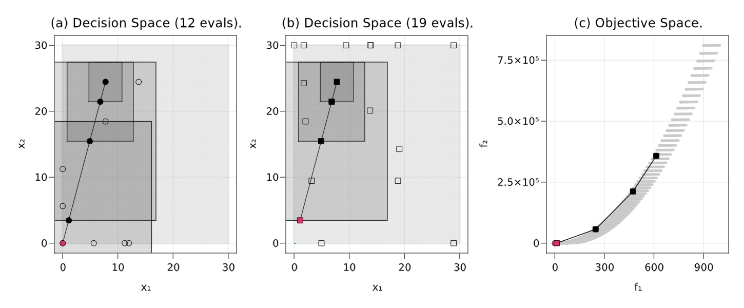
Figure 2: Two runs with maximum number of expensive evaluations set to 20 (soft limit). Test points are light-gray, the iterates are black, final iterate is red, white markers show other points where the objectives are evaluated. The successive trust regions are also shown. (a) Using RBF surrogate models we converge to the optimum using only 12 expensive evaluations. (b) Quadratic Lagrange models do not reach the optimum using 19 evaluations. (c) Iterations and test points in the objective space.

Parameters for Fig. 2, radii relative to $[0,1]^{n}$.

The first objective function is treated as expensive while the second is cheap. The only Pareto-optimal point of (T6) is $[\varepsilon,0]^{T}$. When we set a very restrictive limit of $\mathrm{N}_{\mathrm{exp.}}=20$ then we run out of budget with second degree Lagrange surrogates before we reach the optimum, see Fig. 2 (b). As evident in Fig. 2 (a), surrogates based on (cubic) RBF do require significantly less training data. For the RBF models the algorithm stopped after $2$ critical loops and the model refinement during these loops is made clear by the samples on the problem boundary converging to zero. The complete set of relevant parameters for the test runs is given in Fig. 2. We used a strict acceptance test and the strict Pareto-Cauchy step.

[htb] $\varepsilon_{\mathrm{crit}}$ $\mathrm{N}_{\mathrm{exp.}}$ $\mathrm{N}_{\mathrm{loops}}$ $\mu$ $\beta$ ${\Delta}^{\mathrm{ub}}$ $\Delta_{\mathrm{min}}$ $\Delta^{(0)}$ $\nu_{\scriptscriptstyle+}$ $\nu_{{\scriptscriptstyle++}}$ $\gamma_{\scriptscriptstyle\downdownarrows}$ $\gamma_{\scriptscriptstyle\downarrow}$ $\gamma_{\scriptscriptstyle\uparrow}$ $10^{-3}$ $20$ $2$ $2\cdot 10^{3}$ $10^{3}$ $0.5$ $10^{-3}$ $0.1$ $0.1$ $0.4$ $0.51$ $0.75$ $2$

7.3 Benchmarks on Scalable Test-Problems

To assess the performance with a growing number of decision variables $n$, we performed tests on scalable problems of the ZDT and DTLZ family Zitzler et al. (2000); Deb et al. (2005). Fig. 3 shows results for the bi-objective problems ZDT1-ZDT3 and for the $k$-objective problems DTLZ1 and DTLZ6 (we used $k=\max\{2,n-4\}$ objectives). All problems are box constrained. Eight feasible starting points were generated for each problem setting, i.e., for each combination of $n$, a test problem and a descent method).

In all cases the first objective was considered cheap and all other objectives expensive. First and second degree Lagrange models were compared against linear Taylor models and (cubic) RBF surrogates. The Lagrange models were built using a $\Lambda$-poised set, with $\Lambda=1.5$. In the case of quadratic models we used a precomputed set of points for $n\geq 6$. The Taylor models used finite differences and points outside of box constraints were simply projected back onto the boundary. The RBF models were allowed to include up to $(n+1)(n+2)/2$ training points from the database if $n\leq 10$ and else the maximum number of points was $2n+1$. All other parameters are listed in Section 7.3.

[H] Parameters for Fig. 3, radii relative to $[0,1]^{n}$. $\theta_{1}$ is used to construct Lagrange and RBF models in an enlarged trust region, $\theta_{2}$ is used only for RBF, see Section 4.3. Parameter $\varepsilon_{\mathrm{crit}}$ $\mathrm{N}_{\mathrm{it.}}$ $\mathrm{N}_{\mathrm{exp.}}$ $\mathrm{N}_{\mathrm{loops}}$ $\mu$ $\beta$ ${\Delta}^{\mathrm{ub}}$ $\Delta_{\mathrm{crit}}$ $\varepsilon_{\mathrm{rel}}$ $\Delta_{\mathrm{min}}$ $\Delta^{(0)}$ Value $10^{-3}$ $100$ $n^{2}\cdot 10^{3}$ $10$ $2\cdot 10^{3}$ $10^{3}$ $0.5$ $10^{-3}$ $10^{-8}$ $10^{-6}$ $0.1$ Parameter $\nu_{\scriptscriptstyle+}$ $\nu_{{\scriptscriptstyle++}}$ $\gamma_{\scriptscriptstyle\downdownarrows}$ $\gamma_{\scriptscriptstyle\downarrow}$ $\gamma_{\scriptscriptstyle\uparrow}$ $\theta_{2}$ $\theta_{1}$ Value $0.0$ $0.4$ $0.51$ $0.75$ $2$ $5$ $2$

As expected, the second degree Lagrange polynomials require the most objective evaluations and the quadratic dependence on $n$ is clearly visible in Fig. 3, and the quadratic growth of the dark-blue line continues for $n\geq 8$. On average, the Taylor models perform better than the linear Lagrange polynomials – despite requiring more evaluations per iteration. This is possibly due to more accurate derivative information and resulting faster convergence. The Lagrange models do slightly better when the Pascoletti-Serafini step calculation is used (see Appendix B). By far the least evaluations are needed for the RBF models: The light-blue line consistently stays below all other data points. Often, the average number of evaluations is less than half that of the second best method.

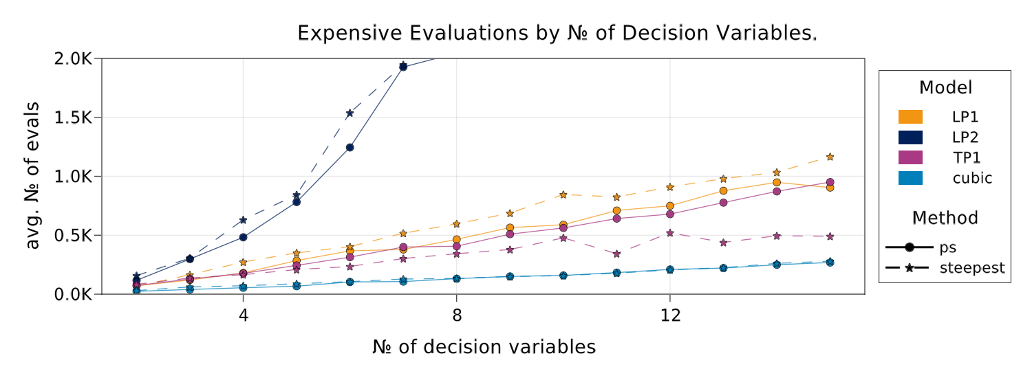
Figure 3: Average number of expensive objective evaluations by number of decision variables $n$, surrogate type and descent method. LP1 are Linear Lagrange models, LP2 quadratic Lagrange models, TP1 are linear Taylor polynomials based on finite differences and cubic refers to cubic RBF models. Steepest descent and Pascoletti-Serafini were tested on scalable problems, and 12 runs were performed per setting.

Fig. 4 illustrates that not only do RBF perform better on average, but also overall. With regards to the final solution criticality, there are a few outliers when the method did not converge using RBF models. However, in most cases the solution criticality is acceptable, see Fig. 4 (b). Moreover, Fig. 5 shows that a good percentage of problem instances is solved with RBF, especially when compared to linear Lagrange polynomial models. Note, that in cases where the true objectives are not differentiable at the final iterate, $\omega$ was set to 0 because the selected problems are non-differentiable only in Pareto-optimal points.

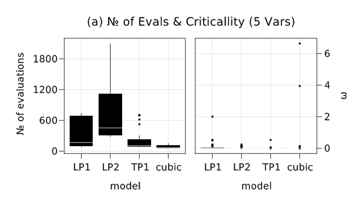
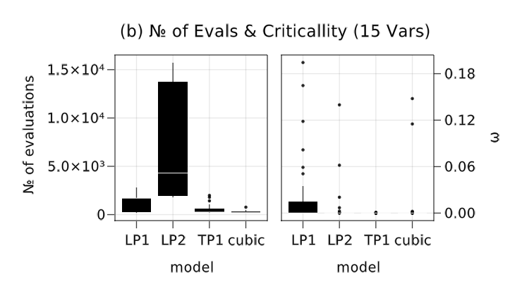
Figure 4: Box-plots of the number of evaluations and the solution criticality for $n=5$ and $n=15$ for the steepest-descent runs from Fig. 3.

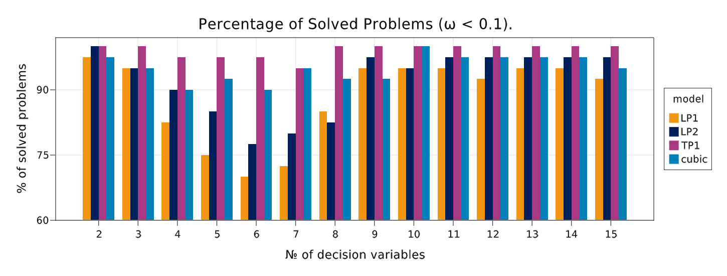
Figure 5: Percentage of solved problem instances, i.e., test runs were the final solution criticality has a value below 0.1. Per model and $n$-value there were 40 runs.

Furthermore, we compared the RBF kernels from Section 4.3. In Wild et al. , the cubic kernel performs best on single-objective problems while the Gaussian does worst. As can be seen in Fig. 6 this holds for multiple objective functions, too. The dark-blue and the light-blue bars show that both the Gaussian and the Multiquadric require more function evaluations, especially in higher dimensions. If, however, we use a very simple adaptive strategy to fine-tune the shape parameter, then both kernels can finish significantly faster. The pink and the gray bar illustrate this fact. In both cases, the shape parameter was set to $\alpha=20/\Delta^{(t)}$ in each iteration. Nevertheless, cubic function (orange) appears to be a good choice in general.

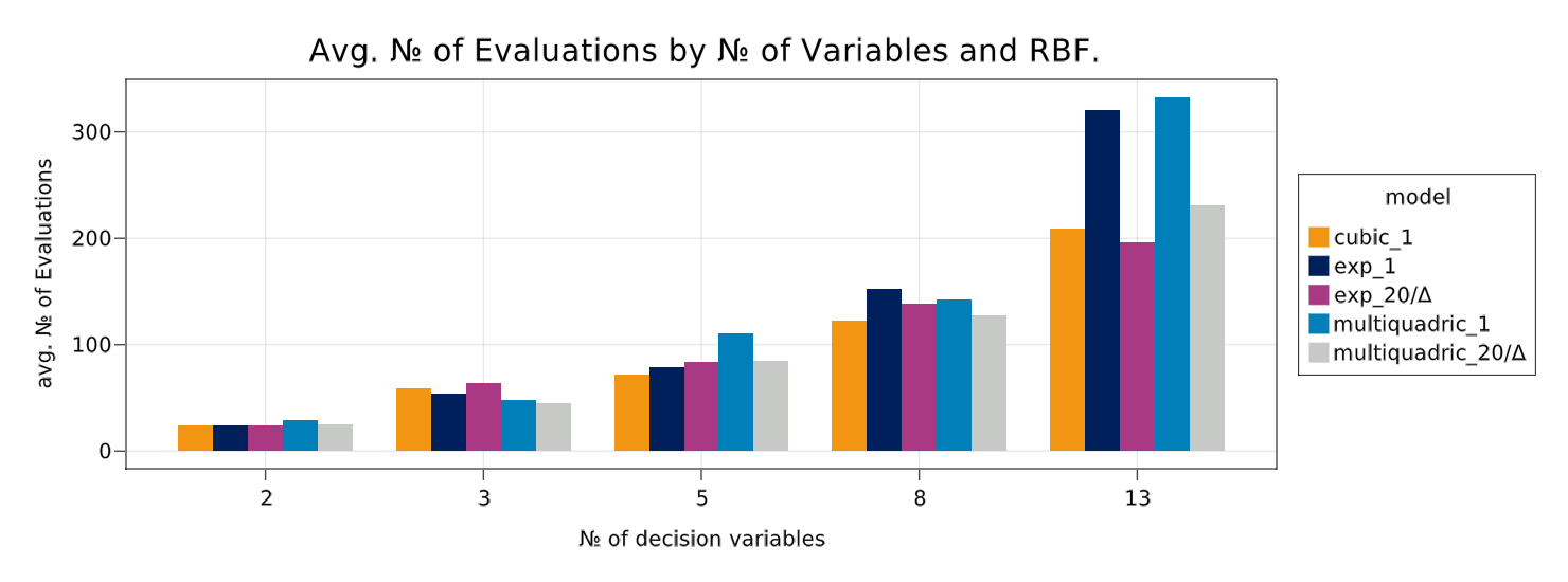
Figure 6: Influence of a adaptive shape radius on the performance of RBF models (tested on ZDT3).

8 Conclusion

We have developed a trust region framework for heterogeneous and expensive multiobjective optimization problems. It is based on similar work Qu et al. ; Villacorta et al. ; Ryu and Kim (2014); Thomann and Eichfelder and our main contributions are the integration of constraints and of radial basis function surrogates. Subsequently, our method is is provably convergent for unconstrained problems and when the feasible set is convex and compact, while requiring significantly less expensive function evaluations due to a linear scaling of complexity with respect to the number of decision variables.

For future work, several modifications and extensions can likely be transferred from the single-objective to the multiobjective case. For examples, the trust region update can be made step-size-dependent (rather than $\rho^{(t)}$ alone) to allow for a more precise model refinement, see (Conn et al., b, Ch. 10). We have also experimented with the nonlinear CG method Lucambio Pérez and Prudente (a) for a multiobjective Steihaug—Toint step (Conn et al., b, Ch. 7) and early results look promising.

Going forward, we would like to apply our algorithm to a real world application, similar to what has been done in Prinz et al. (2020). Moreover, it would be desirable to obtain not just one but multiple Pareto-critical solutions. Because the Pascoletti-Serafini scalarization is still compatible with constraints, the iterations can be guided in image space by providing different global utopia vectors. Furthermore, it is straightforward to use RBF with the heuristic methods from Thomann and Eichfelder (2019) for heterogeneous problems. We believe that it should also be possible to propagate multiple solutions and combine the TRM method with non-dominance testing as has been done in the bi-objective case Ryu and Kim (2014). One can think of other globalization strategies as well: RBF models have been used in multiobjective Stochastic Search algorithms Regis (2016) and trust region ideas have been included into population based strategies Roy et al. (2019). It will thus bee interesting to see whether the theoretical convergence properties can be maintained within these contexts by employing a careful trust-region management. Finally, re-using the data sampled near the final iterate within a continuation framework like in Schütze et al. (2020) is a promising next step.

Conceptualization, M.B. and S.P.; methodology, M.B.; software, M.B.; validation, M.B. and S.P.; formal analysis, M.B. and S.P.; investigation, M.B.; writing—original draft preparation, M.B.; writing—review and editing, S.P.; visualization, M.B.; supervision, S.P.; All authors have read and agreed to the published version of the manuscript.

This research has been funded by the European Union and the German Federal State of North Rhine-Westphalia within the EFRE.NRW project “SET CPS”.

“The authors declare no conflict of interest.”

yes

Appendix A Miscellaneous Proofs

A.1 Continuity of the Constrained Optimal Value

In this subsection we show the continuity of $\omega\left(\bm{\mathrm{x}}\right)$ in the constrained case, where $\omega\left(\bm{\mathrm{x}}\right)$ is the negative optimal value of (P1), i.e.,

$$\omega\left(\bm{\mathrm{x}}\right):= -\min_{\bm{\mathrm{d}}\in\mathcal{X}-\bm{\mathrm{x}}}\max_{\ell=1,\ldots,k}\langle\bm{\nabla}f_{\ell}(\bm{\mathrm{x}}),\bm{\mathrm{d}}\rangle,$$

$$\text{s.t.}\;\left\|\bm{\mathrm{d}}\right\|\leq 1.$$

The proof of the continuity of $\omega\left(\bm{\mathrm{x}}\right)$, as stated in Section 2, follows the reasoning from Fukuda and Drummond , where continuity is shown for a related constrained descent direction program.

Proof of Item 2 in Section 2.

Let the requirements of Item 1 be fulfilled, i.e., let $\bm{\mathrm{f}}$ be continuously differentiable and let $\mathcal{X}\subset\mathbb{R}^{n}$ be convex and compact. Further, let $\bm{\mathrm{x}}$ be a point in $\mathcal{X}$ and denote the minimizing direction in (P1) by $\bm{\mathrm{d}}(\bm{\mathrm{x}})$ and the optimal value by $\theta(\bm{\mathrm{x}})$. We show that $\theta(\bm{\mathrm{x}})$ is continuous, by which $\omega\left(\bm{\mathrm{x}}\right)=-\theta(\bm{\mathrm{x}})$ is continuous as well.

First, note the following properties of the maximum function:

1. $\bm{\mathrm{u}}\mapsto\max_{\ell}u_{\ell}$ is positively homogenous and hence

   $$\max_{\ell}\left(\langle\bm{\nabla}f_{\ell}(\bm{\mathrm{x}}),\bm{\mathrm{d}}_{1}\rangle+\langle\bm{\nabla}f_{\ell}(\bm{\mathrm{x}}),\bm{\mathrm{d}}_{2}\rangle\right)\leq\max_{\ell}\langle\bm{\nabla}f_{\ell}(\bm{\mathrm{x}}),\bm{\mathrm{d}}_{1}\rangle+\max_{\ell}\langle\bm{\nabla}f_{\ell}(\bm{\mathrm{x}}),\bm{\mathrm{d}}_{2}\rangle.$$

2. $\bm{\mathrm{u}}\mapsto\max_{\ell}u_{\ell}$ is Lipschitz with constant 1 so that

   $$\left|\max_{\ell}\langle\bm{\nabla}f(\bm{\mathrm{x}}_{1}),\bm{\mathrm{d}}_{1}\rangle-\max_{\ell}\langle\bm{\nabla}f(\bm{\mathrm{x}}_{2}),\bm{\mathrm{d}}_{2}\rangle\right|\leq\left\|{\bm{\mathrm{D}}{\bm{\mathrm{f}}}}_{\ell}(\bm{\mathrm{x}}_{1})\bm{\mathrm{d}}_{1}-{\bm{\mathrm{D}}{\bm{\mathrm{f}}}}_{\ell}(\bm{\mathrm{x}}_{2})\bm{\mathrm{d}}_{2}\right\|,$$

   for both the maximum and the Euclidean norm.

Now let $\{\bm{\mathrm{x}}^{(t)}\}\subseteq\mathcal{X}$ be a sequence with $\bm{\mathrm{x}}^{(t)}\to\bm{\mathrm{x}}$. Due to the constraints, we have that $\bm{\mathrm{d}}(\bm{\mathrm{x}})\in\mathcal{X}-\bm{\mathrm{x}}$ and thereby $\bm{\mathrm{d}}(\bm{\mathrm{x}})+\bm{\mathrm{x}}-\bm{\mathrm{x}}^{(t)}\in\mathcal{X}-\bm{\mathrm{x}}^{(t)}$. Let

$$(0,1]\ni\sigma^{(t)}:=\begin{cases}\min\left\{1,\dfrac{1}{\left\|\bm{\mathrm{d}}(\bm{\mathrm{x}})+\bm{\mathrm{x}}-\bm{\mathrm{x}}^{(t)}\right\|}\right\}&\text{if $\bm{\mathrm{d}}(\bm{\mathrm{x}})\neq\bm{\mathrm{x}}^{(t)}-\bm{\mathrm{x}}$},\\ 1&\text{else.}\end{cases}$$

Then $\sigma^{(t)}\left(\bm{\mathrm{d}}(\bm{\mathrm{x}})+\bm{\mathrm{x}}-\bm{\mathrm{x}}^{(t)}\right)$ is feasible for (P1) at $\bm{\mathrm{x}}^{(t)}$:

• $\sigma^{(t)}\left(\bm{\mathrm{d}}(\bm{\mathrm{x}})+\bm{\mathrm{x}}-\bm{\mathrm{x}}^{(t)}\right)\in\mathcal{X}-\bm{\mathrm{x}}^{(t)}$ because $\mathcal{X}-\bm{\mathrm{x}}^{(t)}$ is convex and $\bm{\mathrm{0}},\left(\bm{\mathrm{d}}(\bm{\mathrm{x}})+\bm{\mathrm{x}}-\bm{\mathrm{x}}^{(t)}\right)\in\mathcal{X}-\bm{\mathrm{x}}^{(t)}$ as well as $\sigma^{(t)}\in(0,1]$.

• $\left\|\sigma^{(t)}\left(\bm{\mathrm{d}}(\bm{\mathrm{x}})+\bm{\mathrm{x}}-\bm{\mathrm{x}}^{(t)}\right)\right\|\leq 1$ by the definition of $\sigma^{(t)}$.

By the definition of (P1) it follows that

$$\max_{\ell}\langle\bm{\nabla}f_{\ell}(\bm{\mathrm{x}}^{(t)}),\bm{\mathrm{d}}(\bm{\mathrm{x}}^{(t)})\rangle \leq\sigma^{(t)}\max_{\ell}\langle\bm{\nabla}f_{\ell}(\bm{\mathrm{x}}^{(t)}),\bm{\mathrm{d}}(\bm{\mathrm{x}})+\bm{\mathrm{x}}-\bm{\mathrm{x}}^{(t)}\rangle$$

and by Item 1

$$\max_{\ell}\langle\bm{\nabla}f_{\ell}(\bm{\mathrm{x}}^{(t)}),\bm{\mathrm{d}}(\bm{\mathrm{x}}^{(t)})\rangle \leq\sigma^{(t)}\max_{\ell}\langle\bm{\nabla}f_{\ell}(\bm{\mathrm{x}}^{(t)}),\bm{\mathrm{d}}(\bm{\mathrm{x}})\rangle+\sigma^{(t)}\max_{\ell}\langle\bm{\nabla}f_{\ell}(\bm{\mathrm{x}}^{(t)}),\bm{\mathrm{x}}-\bm{\mathrm{x}}^{(t)}\rangle.$$ (32)

We make the following observations:

• Because of $\left\|\bm{\mathrm{d}}(\bm{\mathrm{x}})+\bm{\mathrm{x}}-\bm{\mathrm{x}}^{(t)}\right\|\xrightarrow{t\to\infty}\left\|\bm{\mathrm{d}}(\bm{\mathrm{x}})\right\|\leq 1$, it follows that $\sigma^{(t)}\xrightarrow{t\to\infty}1$.

• Because all objective gradients are continuous, it holds for all $\ell\in\{1,\ldots,k\}$ that $\bm{\nabla}f_{\ell}(\bm{\mathrm{x}}^{(t)})\to\bm{\nabla}f_{\ell}(\bm{\mathrm{x}})$ and because $\bm{\mathrm{u}}\mapsto\max_{\ell}u_{\ell}$ is continuous as well, it then follows that

  $$\max_{\ell}\langle\bm{\nabla}f_{\ell}(\bm{\mathrm{x}}^{(t)}),\bm{\mathrm{d}}(\bm{\mathrm{x}})\rangle\to\max_{\ell}\langle\bm{\nabla}f_{\ell}(\bm{\mathrm{x}}),\bm{\mathrm{d}}(\bm{\mathrm{x}})\rangle\quad\text{for $t\to\infty$.}$$

• The last term on the RHS of (32) vanishes for $t\to\infty$.

By taking the limit superior on (32), we then find that

$$\limsup_{t\to\infty}\theta(\bm{\mathrm{x}}^{(t)})=\limsup_{t\to\infty}\max_{\ell}\langle\bm{\nabla}f_{\ell}(\bm{\mathrm{x}}^{(t)}),\bm{\mathrm{d}}(\bm{\mathrm{x}}^{(t)})\rangle\leq\max_{\ell}\langle\bm{\nabla}f_{\ell}(\bm{\mathrm{x}}),\bm{\mathrm{d}}(\bm{\mathrm{x}})\rangle=\theta(\bm{\mathrm{x}})$$ (33)

Vice versa, we know that because of $\bm{\mathrm{d}}(\bm{\mathrm{x}}^{(t)})\in\mathcal{X}-\bm{\mathrm{x}}^{(t)}$, it holds that $\bm{\mathrm{d}}(\bm{\mathrm{x}}^{(t)})+\bm{\mathrm{x}}^{(t)}-\bm{\mathrm{x}}\in\mathcal{X}-\bm{\mathrm{x}}$ and as above we find that

$$\max_{\ell}\langle\bm{\nabla}f_{\ell}(\bm{\mathrm{x}}),\bm{\mathrm{d}}(\bm{\mathrm{x}})\rangle\leq\lambda^{(t)}\max_{\ell}\langle\bm{\nabla}f_{\ell}(\bm{\mathrm{x}}),\bm{\mathrm{d}}(\bm{\mathrm{x}}^{(t)})\rangle+\lambda^{(t)}\max_{\ell}\langle\bm{\nabla}f_{\ell}(\bm{\mathrm{x}}),\bm{\mathrm{x}}^{(t)}-\bm{\mathrm{x}}\rangle$$ (34)

with

$$\lambda^{(t)}:=\begin{cases}\min\left\{1,\dfrac{1}{\left\|\bm{\mathrm{d}}(\bm{\mathrm{x}})+\bm{\mathrm{x}}^{(t)}-\bm{\mathrm{x}}\right\|}\right\}&\text{if $\bm{\mathrm{d}}(\bm{\mathrm{x}})\neq\bm{\mathrm{x}}^{(t)}-\bm{\mathrm{x}}$},\\ 1&\text{else.}\end{cases}$$

Again, the last term of (34) vanishes in the limit so that by using the properties of the maximum function and the continuity of $\bm{\nabla}f_{\ell}$, as well as $\lambda^{(t)}\xrightarrow{t\to\infty}1$, in taking the limit inferior on (34) we find that

$$\theta(\bm{\mathrm{x}})=\max_{\ell}\langle\bm{\nabla}f_{\ell}(\bm{\mathrm{x}}),\bm{\mathrm{d}}(\bm{\mathrm{x}})\rangle\leq\liminf_{t\to\infty}\max_{\ell}\langle\bm{\nabla}f_{\ell}(\bm{\mathrm{x}}),\bm{\mathrm{d}}(\bm{\mathrm{x}}^{(t)})\rangle$$

$$\leq\liminf_{t\to\infty}\left[\left(\max_{\ell}\langle\bm{\nabla}f_{\ell}(\bm{\mathrm{x}}),\bm{\mathrm{d}}(\bm{\mathrm{x}}^{(t)})\rangle-\max_{\ell}\langle\bm{\nabla}f_{\ell}(\bm{\mathrm{x}}^{(t)}),\bm{\mathrm{d}}(\bm{\mathrm{x}}^{(t)})\rangle\right)+\max_{\ell}\langle\bm{\nabla}f_{\ell}(\bm{\mathrm{x}}^{(t)}),\bm{\mathrm{d}}(\bm{\mathrm{x}}^{(t)})\rangle\right]$$

$$\leq\liminf_{t\to\infty}\left[\left\|{\bm{\mathrm{D}}{\bm{\mathrm{f}}}}(\bm{\mathrm{x}})-{\bm{\mathrm{D}}{\bm{\mathrm{f}}}}(\bm{\mathrm{x}}^{(t)})\right\|\left\|\bm{\mathrm{d}}(\bm{\mathrm{x}}^{(t)})\right\|+\max_{\ell}\langle\bm{\nabla}f_{\ell}(\bm{\mathrm{x}}^{(t)}),\bm{\mathrm{d}}(\bm{\mathrm{x}}^{(t)})\rangle\right]$$

$$\leq\liminf_{t\to\infty}\max_{\ell}\langle\bm{\nabla}f_{\ell}(\bm{\mathrm{x}}^{(t)}),\bm{\mathrm{d}}(\bm{\mathrm{x}}^{(t)})\rangle=\liminf_{t\to\infty}\theta(\bm{\mathrm{x}}^{(t)}).$$ (35)

Combining (33) and (35) shows that $\theta(\bm{\mathrm{x}}^{(t)})\xrightarrow{t\to\infty}\theta(\bm{\mathrm{x}})$. ∎

Section 2 claims that $\omega\left(\bm{\mathrm{x}}\right)$ is uniformly continuous, provided the objective gradients are Lipschitz. The implied Cauchy continuity is an important property in the convergence proof of the algorithm.

Proof of Section 2.

We will consider the constrained case only, when $\mathcal{X}$ is convex and compact and show uniform continuity a fortiori by proving that $\omega\left(\bullet\right)$ is Lipschitz. Let the objective gradients be Lipschitz continuous. Then ${\bm{\mathrm{D}}{\bm{\mathrm{f}}}}$ is Lipschitz as well with constant $L>0$. Let $\bm{\mathrm{x}},\bm{\mathrm{y}}\in\mathcal{X}$ with $\bm{\mathrm{x}}\neq\bm{\mathrm{y}}$ (the other case is trivial) and let again $\bm{\mathrm{d}}(\bm{\mathrm{x}}),\bm{\mathrm{d}}(\bm{\mathrm{y}})$ be the respective optimizers.

Suppose w.l.o.g. that

$$\left|\max_{\ell}\langle\bm{\nabla}f_{\ell}(\bm{\mathrm{x}}),\bm{\mathrm{d}}(\bm{\mathrm{x}})\rangle-\max_{\ell}\langle\bm{\nabla}f_{\ell}(\bm{\mathrm{y}}),\bm{\mathrm{d}}(\bm{\mathrm{y}})\rangle\right| =\max_{\ell}\langle\bm{\nabla}f_{\ell}(\bm{\mathrm{x}}),\bm{\mathrm{d}}(\bm{\mathrm{x}})\rangle-\max_{\ell}\langle\bm{\nabla}f_{\ell}(\bm{\mathrm{y}}),\bm{\mathrm{d}}(\bm{\mathrm{y}})\rangle$$

If we define

$$(0,1]\ni\sigma:=\begin{cases}\min\left\{1,\frac{1}{\left\|\bm{\mathrm{d}}(\bm{\mathrm{y}})+\bm{\mathrm{y}}-\bm{\mathrm{x}}\right\|}\right\}&\text{if $\bm{\mathrm{d}}(\bm{\mathrm{y}})\neq\bm{\mathrm{x}}-\bm{\mathrm{y}}$,}\\ 1&\text{else,}\end{cases}$$

then again $\sigma\left(\bm{\mathrm{d}}(\bm{\mathrm{y}})+\bm{\mathrm{y}}-\bm{\mathrm{x}}\right)$ is feasible for (P1) at $\bm{\mathrm{y}}$. Thus,

$$\max_{\ell}\langle\bm{\nabla}f_{\ell}(\bm{\mathrm{x}}),\bm{\mathrm{d}}(\bm{\mathrm{x}})\rangle-\max_{\ell}\langle\bm{\nabla}f_{\ell}(\bm{\mathrm{y}}),\bm{\mathrm{d}}(\bm{\mathrm{y}})\rangle$$

$$\stackrel{{\scriptstyle\text{df.}}}{{\leq}}\max_{\ell}\langle\bm{\nabla}f_{\ell}(\bm{\mathrm{x}}),\sigma\left(\bm{\mathrm{d}}(\bm{\mathrm{y}})+\bm{\mathrm{y}}-\bm{\mathrm{x}}\right)\rangle-\max_{\ell}\langle\bm{\nabla}f_{\ell}(\bm{\mathrm{y}}),\bm{\mathrm{d}}(\bm{\mathrm{y}})\rangle$$

$$\leq\left\|\sigma{\bm{\mathrm{D}}{\bm{\mathrm{f}}}}(\bm{\mathrm{x}})\left(\bm{\mathrm{d}}(\bm{\mathrm{y}})+\bm{\mathrm{y}}-\bm{\mathrm{x}}\right)-{\bm{\mathrm{D}}{\bm{\mathrm{f}}}}(\bm{\mathrm{y}})\bm{\mathrm{d}}(\bm{\mathrm{y}})\right\|$$

$$\stackrel{{\scriptstyle\sigma\leq 1}}{{\leq}}\left\|\sigma{\bm{\mathrm{D}}{\bm{\mathrm{f}}}}(\bm{\mathrm{x}})-{\bm{\mathrm{D}}{\bm{\mathrm{f}}}}(\bm{\mathrm{y}})\right\|\left\|\bm{\mathrm{d}}(\bm{\mathrm{y}})\right\|+\left\|{\bm{\mathrm{D}}{\bm{\mathrm{f}}}}(\bm{\mathrm{x}})\right\|\left\|\bm{\mathrm{x}}-\bm{\mathrm{y}}\right\|,$$ (36)

where we have again used Item 2 for the second inequality. We now investigate the first term on the RHS. Using $\left\|\bm{\mathrm{d}}(\bm{\mathrm{y}})\right\|\leq 1$ and adding a zero, we find

$$\left\|\sigma{\bm{\mathrm{D}}{\bm{\mathrm{f}}}}(\bm{\mathrm{x}})-{\bm{\mathrm{D}}{\bm{\mathrm{f}}}}(\bm{\mathrm{y}})\right\|\left\|\bm{\mathrm{d}}(\bm{\mathrm{y}})\right\| \leq\left\|{\bm{\mathrm{D}}{\bm{\mathrm{f}}}}(\bm{\mathrm{x}})-{\bm{\mathrm{D}}{\bm{\mathrm{f}}}}(\bm{\mathrm{y}})-(1-\sigma){\bm{\mathrm{D}}{\bm{\mathrm{f}}}}(\bm{\mathrm{x}})\right\|$$

$$\leq L\left\|\bm{\mathrm{x}}-\bm{\mathrm{y}}\right\|+(1-\sigma)\left\|{\bm{\mathrm{D}}{\bm{\mathrm{f}}}}(\bm{\mathrm{x}})\right\|.$$ (37)

Furthermore, $\left\|\bm{\mathrm{d}}(\bm{\mathrm{y}})+\bm{\mathrm{y}}-\bm{\mathrm{x}}\right\|\leq 1+\left\|\bm{\mathrm{y}}-\bm{\mathrm{x}}\right\|$ implies $1/(1+\left\|\bm{\mathrm{y}}-\bm{\mathrm{x}}\right\|)\leq\sigma$ and

$$1-\sigma\leq 1-\frac{1}{1+\left\|\bm{\mathrm{y}}-\bm{\mathrm{x}}\right\|}=\frac{\left\|\bm{\mathrm{y}}-\bm{\mathrm{x}}\right\|}{1+\left\|\bm{\mathrm{y}}-\bm{\mathrm{x}}\right\|}\leq\left\|\bm{\mathrm{y}}-\bm{\mathrm{x}}\right\|.$$

We use this inequality and plug (37) into (36) to obtain

$$\max_{\ell}\langle\bm{\nabla}f_{\ell}(\bm{\mathrm{x}}),\bm{\mathrm{d}}(\bm{\mathrm{x}})\rangle-\max_{\ell}\langle\bm{\nabla}f_{\ell}(\bm{\mathrm{y}}),\bm{\mathrm{d}}(\bm{\mathrm{y}})\rangle \leq L\left\|\bm{\mathrm{x}}-\bm{\mathrm{y}}\right\|+2\left\|{\bm{\mathrm{D}}{\bm{\mathrm{f}}}}(\bm{\mathrm{x}})\right\|\left\|\bm{\mathrm{x}}-\bm{\mathrm{y}}\right\|$$

$$\leq(L+2D)\left\|\bm{\mathrm{x}}-\bm{\mathrm{y}}\right\|,$$

with $D=\max_{\bm{\mathrm{x}}\in\mathcal{X}}\left\|{\bm{\mathrm{D}}{\bm{\mathrm{f}}}}(\bm{\mathrm{x}})\right\|$ which is well defined because $\mathcal{X}$ is compact and $\left\|{\bm{\mathrm{D}}{\bm{\mathrm{f}}}}({\bullet})\right\|$ is continuous. ∎

A.2 Modified Criticality Measures

Proof of Section 5.3.

There are two cases to consider:

• If $\omega_{\mathrm{m}}^{(t)}\left(\bm{\mathrm{x}}^{(t)}\right)\geq\omega\left(\bm{\mathrm{x}}^{(t)}\right)$ then

  $$\left|\omega_{\mathrm{m}}^{(t)}\left(\bm{\mathrm{x}}^{(t)}\right)-\omega\left(\bm{\mathrm{x}}^{(t)}\right)\right|=\omega_{\mathrm{m}}^{(t)}\left(\bm{\mathrm{x}}^{(t)}\right)-\omega\left(\bm{\mathrm{x}}^{(t)}\right)\leq\kappa_{\omega}\omega_{\mathrm{m}}^{(t)}\left(\bm{\mathrm{x}}^{(t)}\right).$$

  Now

  $${\left|\varpi_{\mathrm{m}}^{(t)}\left(\bm{\mathrm{x}}^{(t)}\right)-\varpi\left(\bm{\mathrm{x}}^{(t)}\right)\right|\in}\left\{\begin{aligned} &\phantom{{}\leq{}}\omega_{\mathrm{m}}^{(t)}\left(\bm{\mathrm{x}}^{(t)}\right)-\omega\left(\bm{\mathrm{x}}^{(t)}\right)\\ 1-\omega\left(\bm{\mathrm{x}}^{(t)}\right)&\leq\omega_{\mathrm{m}}^{(t)}\left(\bm{\mathrm{x}}^{(t)}\right)-\omega\left(\bm{\mathrm{x}}^{(t)}\right)\\ 1-1&=0\end{aligned}\right\}\leq\kappa_{\omega}\omega_{\mathrm{m}}^{(t)}\left(\bm{\mathrm{x}}^{(t)}\right).$$

• The case $\omega\left(\bm{\mathrm{x}}^{(t)}\right)<\omega_{\mathrm{m}}^{(t)}\left(\bm{\mathrm{x}}^{(t)}\right)$ can be shown similarly.

∎

Proof of Section 5.3.

Use Section 5.3 and then investigate the two possible cases:

• If $\varpi_{\mathrm{m}}^{(t)}\left(\bm{\mathrm{x}}^{(t)}\right)\geq\varpi\left(\bm{\mathrm{x}}^{(t)}\right)$, then the first inequality follows because of $1\geq 1/(1+\kappa_{\omega})$.

• If $\varpi_{\mathrm{m}}^{(t)}\left(\bm{\mathrm{x}}^{(t)}\right)<\varpi\left(\bm{\mathrm{x}}^{(t)}\right)$, then $\varpi\left(\bm{\mathrm{x}}^{(t)}\right)-\varpi_{\mathrm{m}}^{(t)}\left(\bm{\mathrm{x}}^{(t)}\right)\leq\kappa_{\omega}\varpi_{\mathrm{m}}^{(t)}\left(\bm{\mathrm{x}}^{(t)}\right),$ and again the first inequality follows.

∎

Appendix B Pascoletti-Serafini Step

One example of an alternative descent step $\bm{\mathrm{s}}^{(t)}\in\mathbb{R}^{n}$ is given in Thomann and Eichfelder . Thomann and Eichfelder leverage the Pascoletti-Serafini scalarization to define local subproblems that guide the iterates towards the (local) model ideal point. To be precise, it is shown that the trial point $\bm{\mathrm{x}}_{+}^{(t)}$ can be computed as the solution to

$$\min_{\tau\in\mathbb{R},\bm{\mathrm{x}}\in B^{(t)}}\tau\quad\text{ s.t. }\bm{\mathrm{m}}^{(t)}(\bm{\mathrm{x}}^{(t)})+\tau\bm{\mathrm{r}}^{(t)}-\bm{\mathrm{m}}^{(t)}(\bm{\mathrm{x}})\geq\bm{\mathrm{0}},$$ (38)

where $\bm{\mathrm{r}}^{(t)}=\bm{\mathrm{m}}^{(t)}(\bm{\mathrm{x}}^{(t)})-\bm{\mathrm{i}}_{\mathrm{m}}^{(t)}\in\mathbb{R}^{k}_{\geq 0}$ is the direction vector pointing from the local model ideal point

$$\bm{\mathrm{i}}_{\mathrm{m}}^{(t)}=\begin{bmatrix}i_{1}^{(t)},\ldots,i_{k}^{(t)}\end{bmatrix}^{T},\,\text{ with $i_{\ell}^{(t)}=\min_{\bm{\mathrm{x}}\in\mathcal{X}}m^{(t)}_{\ell}(\bm{\mathrm{x}})$ for $\ell=1,\ldots,k,$}$$ (39)

to the current iterate value. If the surrogates are linear or quadratic polynomials and the trust region use a $p$-norm with $p\in\{1,2,\infty\}$ these sub-problems are linear or quadratic programs.

A convergence proof for the unconstrained case is given in Thomann and Eichfelder . It relies on a sufficient decrease bound similar to (20). However, it is not shown that $\kappa^{\scriptstyle\mathrm{sd}}\in(0,1)$ exists independent of the iteration index $t$ but stated as an assumption.
Furthermore, constraints (in particular box constraints) are integrated into the definition of $\omega\left(\bullet\right)$ and $\omega_{\mathrm{m}}^{(t)}\left(\bullet\right)$ using an active set strategy (see Thomann (2018)). Consequently, both values are no longer Cauchy continuous. We can remedy both drawbacks by relating the (possibly constrained) Pascoletti-Serafini trial point to the strict modified Pareto-Cauchy point in our projection framework. To this end, we allow in (38) and (39) any feasible set fulfilling Section 2. Moreover we recite the following assumption: [Assumption 4.10 in Thomann and Eichfelder ] There is a constant $\mathrm{r}\in(0,1]$ so that if $\bm{\mathrm{x}}^{(t)}$ is not Pareto-critical, the components $r_{1}^{(t)},\ldots,r_{k}^{(t)},$ of $\bm{\mathrm{r}}^{(t)}$ satisfy $\dfrac{\min_{\ell}r_{\ell}^{(t)}}{\max_{\ell}r_{\ell}^{(t)}}\geq\mathrm{r}.$ The assumption can be justified because $r_{\ell}^{(t)}>0$ if $\bm{\mathrm{x}}^{(t)}$ is not critical and $r_{\ell}^{(t)}$ can be bounded above and below by expressions involving $\omega_{\mathrm{m}}^{(t)}\left(\bullet\right)$, see Section 5.1 and (Thomann and Eichfelder, , Lemma 4.9). We can then derive the following lemma: Suppose Sections 2, 5.1 and B hold. Let $(\tau^{+},\bm{\mathrm{x}}_{+}^{(t)})$ be the solution to (38). Then there exists a constant ${\tilde{\kappa}}^{\mathrm{sd}}_{\mathrm{m}}\in(0,1)$ such that it holds

$$\Phi_{\mathrm{m}}^{(t)}(\bm{\mathrm{x}}^{(t)})-\Phi_{\mathrm{m}}^{(t)}(\bm{\mathrm{x}}_{+}^{(t)})\geq{\tilde{\kappa}}^{\mathrm{sd}}_{\mathrm{m}}\omega_{\mathrm{m}}^{(t)}\left(\bm{\mathrm{x}}^{(t)}\right)\min\left\{\frac{\omega_{\mathrm{m}}^{(t)}\left(\bm{\mathrm{x}}^{(t)}\right)}{\mathrm{c}H_{\mathrm{m}}^{(t)}},\Delta^{(t)},1\right\}.$$

Proof.

If $\bm{\mathrm{x}}^{(t)}$ is critical for (MOP$\mathrm{m}$), then $\tau^{+}=0$ and $\bm{\mathrm{x}}_{+}^{(t)}=\bm{\mathrm{x}}^{(t)}$ and the bound is trivial Eichfelder . Otherwise, we can use the same argumentation as in (Thomann and Eichfelder, , Lemma 4.13) to show that for the strict modified Pareto-Cauchy point $\bm{\mathrm{{\hat{x}}}}_{\mathrm{PC}}^{(t)}$ it holds that

$$\Phi_{\mathrm{m}}^{(t)}(\bm{\mathrm{x}}^{(t)})-\Phi_{\mathrm{m}}^{(t)}(\bm{\mathrm{x}}_{+}^{(t)}) \geq\mathrm{r}\min_{\ell}\left\{m^{(t)}_{\ell}(\bm{\mathrm{x}}^{(t)})-m^{(t)}_{\ell}(\bm{\mathrm{{\hat{x}}}}_{\mathrm{PC}}^{(t)})\right\}$$

and the final bound follows from Section 5.2 with the new constant ${\tilde{\kappa}}^{\mathrm{sd}}_{\mathrm{m}}=\mathrm{r}\kappa^{\scriptstyle\mathrm{sd}}_{\mathrm{m}}$. ∎

References

yes

References

- Ehrgott (2005) Ehrgott, M. Multicriteria optimization, 2nd ed ed.; Springer: Berlin ; New York, 2005.
- (2) Jahn, J. Vector optimization: theory, applications, and extensions, 2. ed ed.; Springer. OCLC: 725378304.
- Miettinen (2013) Miettinen, K. Nonlinear Multiobjective Optimization.; Springer Verlag, 2013. OCLC: 1089790877.
- Eichfelder (2020) Eichfelder, G. Twenty Years of Continuous Multiobjective Optimization 2020. p. 34.
- (5) Eichfelder, G. Adaptive Scalarization Methods in Multiobjective Optimization; Vector Optimization, Springer Berlin Heidelberg. doi:\changeurlcolorblack10.1007/978-3-540-79159-1.
- (6) Fukuda, E.H.; Drummond, L.M.G. A SURVEY ON MULTIOBJECTIVE DESCENT METHODS. 34, 585–620. doi:\changeurlcolorblack10.1590/0101-7438.2014.034.03.0585.
- (7) Fliege, J.; Svaiter, B.F. Steepest descent methods for multicriteria optimization. 51, 479–494. doi:\changeurlcolorblack10.1007/s001860000043.
- Graña Drummond and Svaiter (2005) Graña Drummond, L.; Svaiter, B. A steepest descent method for vector optimization. Journal of Computational and Applied Mathematics 2005, 175, 395–414. doi:\changeurlcolorblack10.1016/j.cam.2004.06.018.
- Lucambio Pérez and Prudente (a) Lucambio Pérez, L.R.; Prudente, L.F. Nonlinear Conjugate Gradient Methods for Vector Optimization. 28, 2690–2720. doi:\changeurlcolorblack10.1137/17M1126588.
- Lucambio Pérez and Prudente (b) Lucambio Pérez, L.R.; Prudente, L.F. A Wolfe Line Search Algorithm for Vector Optimization. 45, 1–23. doi:\changeurlcolorblack10.1145/3342104.
- Gebken et al. (2019) Gebken, B.; Peitz, S.; Dellnitz, M. A Descent Method for Equality and Inequality Constrained Multiobjective Optimization Problems. Numerical and Evolutionary Optimization – NEO 2017; Trujillo, L.; Schütze, O.; Maldonado, Y.; Valle, P., Eds. Springer, Cham, 2019, pp. 29–61.
- Hillermeier (2001) Hillermeier, C. Nonlinear multiobjective optimization: a generalized homotopy approach; Springer Basel AG: Basel, 2001. OCLC: 828735498.
- Gebken et al. (2019) Gebken, B.; Peitz, S.; Dellnitz, M. On the hierarchical structure of Pareto critical sets. Journal of Global Optimization 2019, 73, 891–913.
- Wilppu et al. (2014) Wilppu, O.; Karmitsa, N.; Mäkelä, M. New multiple subgradient descent bundle method for nonsmooth multiobjective optimization. Report no., Turku Centre for Computer Science 2014.
- Gebken and Peitz (2021) Gebken, B.; Peitz, S. An Efficient Descent Method for Locally Lipschitz Multiobjective Optimization Problems. Journal of Optimization Theory and Applications 2021. doi:\changeurlcolorblack10.1007/s10957-020-01803-w.
- Custódio et al. (2011) Custódio, A.L.; Madeira, J.F.A.; Vaz, A.I.F.; Vicente, L.N. Direct Multisearch for Multiobjective Optimization. SIAM Journal on Optimization 2011, 21, 1109–1140. doi:\changeurlcolorblack10.1137/10079731x.
- Audet et al. (2008) Audet, C.; Savard, G.; Zghal, W. Multiobjective Optimization Through a Series of Single-Objective Formulations. SIAM J. on Optimization 2008, 19, 188–210. doi:\changeurlcolorblack10.1137/060677513.
- Deb (2001) Deb, K. Multi-Objective Optimization Using Evolutionary Algorithms; Wiley, 2001.
- Coello et al. (2007) Coello, C.A.C.; Lamont, G.B.; Veldhuizen, D.A.V. Evolutionary Algorithms for Solving Multi-Objective Problems Second Edition 2007.
- Abraham et al. (2005) Abraham, A.; Jain, L.C.; Goldberg, R., Eds. Evolutionary multiobjective optimization: theoretical advances and applications; Advanced information and knowledge processing, Springer: New York, 2005.
- (21) Zitzler, E. Evolutionary Algorithms for Multiobjective Optimization: Methods and Applications. p. 134.
- Deb et al. (2002) Deb, K.; Pratap, A.; Agarwal, S.; Meyarivan, T. A fast and elitist multiobjective genetic algorithm: NSGA-II. IEEE Transactions on Evolutionary Computation 2002, 6, 182–197. doi:\changeurlcolorblack10.1109/4235.996017.
- Peitz and Dellnitz (2018) Peitz, S.; Dellnitz, M. A Survey of Recent Trends in Multiobjective Optimal Control—Surrogate Models, Feedback Control and Objective Reduction. Mathematical and Computational Applications 2018, 23, 30. doi:\changeurlcolorblack10.3390/mca23020030.
- Chugh et al. (2019) Chugh, T.; Sindhya, K.; Hakanen, J.; Miettinen, K. A survey on handling computationally expensive multiobjective optimization problems with evolutionary algorithms. Soft Computing 2019, 23, 3137–3166. doi:\changeurlcolorblack10.1007/s00500-017-2965-0.
- Deb et al. (2020) Deb, K.; Roy, P.C.; Hussein, R. Surrogate Modeling Approaches for Multiobjective Optimization: Methods, Taxonomy, and Results. Mathematical and Computational Applications 2020, 26, 5. doi:\changeurlcolorblack10.3390/mca26010005.
- Roy et al. (2019) Roy, P.C.; Hussein, R.; Blank, J.; Deb, K. Trust-Region Based Multi-objective Optimization for Low Budget Scenarios. In Evolutionary Multi-Criterion Optimization; Deb, K.; Goodman, E.; Coello Coello, C.A.; Klamroth, K.; Miettinen, K.; Mostaghim, S.; Reed, P., Eds.; Springer International Publishing: Cham, 2019; Vol. 11411, pp. 373–385. Series Title: Lecture Notes in Computer Science, doi:\changeurlcolorblack10.1007/978-3-030-12598-1_30.
- (27) Conn, A.R.; Scheinberg, K.; Vicente, L.N. Introduction to derivative-free optimization; Number 8 in MPS-SIAM series on optimization, Society for Industrial and Applied Mathematics/Mathematical Programming Society. OCLC: ocn244660709.
- Larson et al. (2019) Larson, J.; Menickelly, M.; Wild, S.M. Derivative-free optimization methods. arXiv:1904.11585 [math] 2019. arXiv: 1904.11585, doi:\changeurlcolorblack10.1017/S0962492919000060.
- (29) Qu, S.; Goh, M.; Liang, B. Trust region methods for solving multiobjective optimisation. 28, 796–811. doi:\changeurlcolorblack10.1080/10556788.2012.660483.
- (30) Villacorta, K.D.V.; Oliveira, P.R.; Soubeyran, A. A Trust-Region Method for Unconstrained Multiobjective Problems with Applications in Satisficing Processes. 160, 865–889. doi:\changeurlcolorblack10.1007/s10957-013-0392-7.
- Ryu and Kim (2014) Ryu, J.h.; Kim, S. A Derivative-Free Trust-Region Method for Biobjective Optimization. SIAM Journal on Optimization 2014, 24, 334–362. doi:\changeurlcolorblack10.1137/120864738.
- (32) Thomann, J.; Eichfelder, G. A Trust-Region Algorithm for Heterogeneous Multiobjective Optimization. 29, 1017–1047. doi:\changeurlcolorblack10.1137/18M1173277.
- (33) Wild, S.M.; Regis, R.G.; Shoemaker, C.A. ORBIT: Optimization by Radial Basis Function Interpolation in Trust-Regions. 30, 3197–3219. doi:\changeurlcolorblack10.1137/070691814.
- Conn et al. (a) Conn, A.R.; Scheinberg, K.; Vicente, L.N. Global Convergence of General Derivative-Free Trust-Region Algorithms to First- and Second-Order Critical Points. 20, 387–415. doi:\changeurlcolorblack10.1137/060673424.
- Conn et al. (b) Conn, A.R.; Gould, N.I.M.; Toint, P.L. Trust-region methods; MPS-SIAM series on optimization, Society for Industrial and Applied Mathematics.
- (36) Luc, D.T. Theory of Vector Optimization; Vol. 319, Lecture Notes in Economics and Mathematical Systems, Springer Berlin Heidelberg. doi:\changeurlcolorblack10.1007/978-3-642-50280-4.
- Thomann (2018) Thomann, J. A Trust Region Approach for Multi-Objective Heterogeneous Optimization 2018. p. 257.
- Wendland (2004) Wendland, H. Scattered Data Approximation, 1 ed.; Cambridge University Press, 2004. doi:\changeurlcolorblack10.1017/CBO9780511617539.
- Stefan (2008) Stefan, W. Derivative-Free Optimization Algorithms For Computationally Expensive Functions 2008.
- (40) Wild, S.M.; Shoemaker, C. Global Convergence of Radial Basis Function Trust Region Derivative-Free Algorithms. 21, 761–781. doi:\changeurlcolorblack10.1137/09074927X.
- Regis and Wild (2017) Regis, R.G.; Wild, S.M. CONORBIT: constrained optimization by radial basis function interpolation in trust regions. Optimization Methods and Software 2017, 32, 552–580. doi:\changeurlcolorblack10.1080/10556788.2016.1226305.
- Fleming (1977) Fleming, W. Functions of Several Variables; Undergraduate Texts in Mathematics, Springer New York: New York, NY, 1977. doi:\changeurlcolorblack10.1007/978-1-4684-9461-7.
- Stellato et al. (2020) Stellato, B.; Banjac, G.; Goulart, P.; Bemporad, A.; Boyd, S. OSQP: an operator splitting solver for quadratic programs. Mathematical Programming Computation 2020, 12, 637–672. doi:\changeurlcolorblack10.1007/s12532-020-00179-2.
- (44) Johnson, S.G. The NLopt nonlinear-optimization package.
- Powell (2009) Powell, M.J. The BOBYQA algorithm for bound constrained optimization without derivatives 2009.
- Legat et al. (2020) Legat, B.; Timme, S.; Weisser, T.; Kapelevich, L.; Rackauckas, C.; TagBot, J. JuliaAlgebra/DynamicPolynomials.jl: v0.3.15, 2020. doi:\changeurlcolorblack10.5281/zenodo.4153432.
- Runarsson and Yao (2005) Runarsson, T.P.; Yao, X. Search biases in constrained evolutionary optimization. IEEE Transactions on Systems, Man, and Cybernetics, Part C (Applications and Reviews) 2005, 35, 233–243.
- Revels et al. (2016) Revels, J.; Lubin, M.; Papamarkou, T. Forward-Mode Automatic Differentiation in Julia. arXiv:1607.07892 [cs.MS] 2016.
- Zitzler et al. (2000) Zitzler, E.; Deb, K.; Thiele, L. Comparison of Multiobjective Evolutionary Algorithms: Empirical Results. Evolutionary Computation 2000, 8, 173–195. doi:\changeurlcolorblack10.1162/106365600568202.
- Deb et al. (2005) Deb, K.; Thiele, L.; Laumanns, M.; Zitzler, E. Scalable Test Problems for Evolutionary Multiobjective Optimization. In Evolutionary Multiobjective Optimization; Abraham, A.; Jain, L.; Goldberg, R., Eds.; Springer-Verlag: London, 2005; pp. 105–145. Series Title: Advanced Information and Knowledge Processing, doi:\changeurlcolorblack10.1007/1-84628-137-7_6.
- Prinz et al. (2020) Prinz, S.; Thomann, J.; Eichfelder, G.; Boeck, T.; Schumacher, J. Expensive multi-objective optimization of electromagnetic mixing in a liquid metal. Optimization and Engineering 2020. doi:\changeurlcolorblack10.1007/s11081-020-09561-4.
- Thomann and Eichfelder (2019) Thomann, J.; Eichfelder, G. Representation of the Pareto front for heterogeneous multi-objective optimization. J. Appl. Numer. Optim 2019, 1, 293–323.
- Regis (2016) Regis, R.G. Multi-objective constrained black-box optimization using radial basis function surrogates. Journal of Computational Science 2016, 16, 140–155. doi:\changeurlcolorblack10.1016/j.jocs.2016.05.013.
- Schütze et al. (2020) Schütze, O.; Cuate, O.; Martín, A.; Peitz, S.; Dellnitz, M. Pareto Explorer: a global/local exploration tool for many-objective optimization problems. Engineering Optimization 2020, 52, 832–855. doi:\changeurlcolorblack10.1080/0305215X.2019.1617286.