Dynamic coarse-graining of polymer systems using mobility functions

Abstract

We propose a dynamic coarse-graining (CG) scheme for mapping heterogeneous polymer fluids onto extremely CG models in a dynamically consistent manner. The idea is to use as target function for the mapping a wave-vector dependent mobility function derived from the single-chain dynamic structure factor, which is calculated in the microscopic reference system. In previous work, we have shown that dynamic density functional calculations based on this mobility function can accurately reproduce the order/disorder kinetics in polymer melts, thus it is a suitable starting point for dynamic mapping. To enable the mapping over a range of relevant wave vectors, we propose to modify the CG dynamics by introducing internal friction parameters that slow down the CG monomer dynamics on local scales, without affecting the static equilibrium structure of the system. We illustrate and discuss the method using the example of infinitely long linear Rouse polymers mapped onto ultrashort CG chains. We show that our method can be used to construct dynamically consistent CG models for homopolymers with CG chain length $N=4$, whereas for copolymers, longer CG chain lengths are necessary.

Keywords: polymer simulations; coarse-graining; dynamics; friction; dynamic structure factor; dynamic density functional theory; mobility

1 Introduction

Mixing polymers of different types is a simple and inexpensive way to create novel materials[1, 2]. However, chemically different polymers usually do not mix well. Polymeric composite materials therefore tend to be heterogeneous on local scales and filled with internal interfaces, which largely determine the resulting material properties[3]. The morphology of the materials depend on the history, i.e., the way they have been processed. Understanding the dynamics of polymer kinetics in inhomogeneous materials is thus crucial if one wants to understand and predict the structure and properties of the resulting materials.

Computer simulations are a powerful tool to study soft matter systems. Due to the large size of the polymers and the even larger typical length scales of the inhomogeneities, simulations in full atomistic details are usually not possible, and using coarse-grained (CG) models instead has a long and successful history[4]. In CG polymer models, monomers or groups of monomers are lumped into one ”bead” of simpler structure. Generic models offer insight into universal features, and specific models with parameters adjusted to concrete molecules are used for quantitative studies. Designing such specific CG models requires the development of mapping procedures that allow to derive the parameters of the CG models from the microscopic static and dynamic features of the target systems [5, 6, 7, 8, 9, 10, 11].

With respect to the static properties of equilibrium systems, such methods are by now well-established. Various protocols have been proposed to derive effective potentials of coarse-grained models from microscopic simulations by analyzing local correlations or force distributions[9, 10]. In addition, established mesoscopic concepts such as the Flory Huggins $\chi$-parameter[2], the statistical segment length[12], or the Maier-Saupe parameter[13, 14, 15] are used to map microscopic models (or experimental data) on continuum models and then back to extremely CG particle-based polymer models[16, 17, 18]. In the latter case, the target quantity in the CG parameter optimization is often the static structure factor, and polymer theories like the random phase approximation (RPA) or the self-consistent field theory (SCF) help to establish the connection between fine-grained and CG models[19, 20, 21].

Motivated by these successes, similar efforts are made to design mapping and CG methods for polymer dynamics. In the earliest and still very popular approach[22, 23], the CG model is simulated by standard molecular dynamics and a single time scale – e.g., the time scale of diffusion – is used to mapped the CG system onto the fine-grained system. However, it has been long known through the work of Mori and Zwanzig[24, 25, 26], that coarse-graining has a much more fundamental effect on the structure of the equations of motion: Integrating out degrees of freedom invariably turns a Hamiltonian system into a dissipative system with memory. Based on this insight, several recent efforts have been devoted to deriving generalized Langevin (GLE) models for polymer melts and solutions, using as target quantities for the mapping the (absolute or relative) velocity autocorrelation function of the center of mass[27, 28, 29, 30, 31] of the molecules. In most of these systems, whole polymer molecules (typically relatively small star polymers) were mapped onto single CG particles. Extending these concepts to CG models that map polymers on CG chains with multiple sites is far from trivial[32, 33, 34]. One approach that has been rather successful in the case of oligomer molecules was to integrate over pair memory kernels and thereby derive dissipative particle dynamics (DPD) friction constants for monomers[35] – similar to earlier work by Hijon et al who used the Mori-Zwanzig formalism to construct DPD equations for CG particles representing whole star polymers[36]. However, it is not clear whether this approach will also work for large molecules, where internal chain motion is a significant source of memory and friction. An alternative route that is closer to the static coarse-graining strategies developed for mesoscopic scales would be to use the dynamic structure factor as a starting point for mapping. Such a strategy will be explored in the present paper.

We target systems containing polymers of large molecular weight, i.e., made of thousands of monomers, and CG strategies that map these molecules onto much shorter chains of soft blobs. The dynamics of such polymers is theoretically described as an overdamped motion in a background medium created by the other polymers, e.g., Rouse, Zimm, or reptation dynamics[12]. Successful static CG strategies are based on ”theoretically informed” soft potentials that are derived from static density functionals[37, 38, 39, 40, 41, 42, 43, 44, 45, 17] and reproduce key quantities such as the $\chi$ parameter. Here we take a similar approach, but use as mesoscopic reference theory the overdamped dynamic density functional theory (DDFT). The standard Ansatz of such a DDFT equation for polymers has the form[46, 47, 48, 49, 50, 51, 52]

$$\frac{\partial\rho_{\alpha}(\mathbf{r},t)}{\partial t}=\sum_{\beta}\nabla_{\mathbf{r}}\left[\int d\mathbf{r}^{\prime}\Lambda_{\alpha\beta}(\mathbf{r},\mathbf{r}^{\prime})\nabla_{\mathbf{r}^{\prime}}\mu_{\beta}(\mathbf{r}^{\prime},t)\right].$$ (1)

Here $\rho_{\alpha}(\mathbf{r},t)$ is the local density of component $\alpha$ at the position $\mathbf{r}$, the quantity $\nabla_{\mathbf{r}^{\prime}}\mu_{\beta}(\mathbf{r}^{\prime},t)$ is the thermodynamic force acting on component $\beta$ at position $\mathbf{r}^{\prime}$, and $\Lambda_{\alpha\beta}(\mathbf{r},\mathbf{r}^{\prime})$ a non-local mobility function that accounts, e.g., for chain connectivity effects. Obviously, Eq. (1) is Markovian and does not include memory effects. More general versions of (1) that includes a memory kernel $K(\mathbf{r},\mathbf{r}^{\prime},t)$ have been proposed by Semenov[53] and more recently by Müller and coworkers[54, 55]. Eq. (1) represents a Markovian approximation to the full GLE which accounts for different relaxation times on different length scales in an effective manner. We will discuss this in more detail in the next section.

In previous work, we have devised a way to extract mobility functions in polymer systems in a bottom-up fashion from fine-grained simulations, using as input data the single chain dynamics structure factor, $g(\mathbf{q},t)=\frac{1}{N}\langle\sum_{n,m=1}^{N}\mathrm{e}^{i\mathbf{q}\cdot(\mathbf{R}_{n}(t)-\mathbf{R}_{m}(0))}\rangle$, where the sum $n,m$ runs over all $N$ monomers of the chain, and $\mathbf{R}_{n}(t)$ is the position of monomer $n$ at time $t$. Knowing $g(\mathbf{q},t)$, one can calculate the rescaled single-chain mobility[56] in Fourier space as

$$\hat{\Lambda}(\mathbf{q})=\frac{1}{k_{{}_{B}}TN^{2}}\>g(\mathbf{q},0)G^{-1}(\mathbf{q})\>g(\mathbf{q},0)\quad\mbox{with}\quad G(\mathbf{q})=\frac{q^{2}}{N}\int_{0}^{\infty}\mathrm{d}t\>g(\mathbf{q},t)$$ (2)

In a homopolymer mixture containing polymers of type $\alpha$ (length $N_{\alpha}$) in the number concentration $c_{\alpha}$, the total mobility function is then given by[56]

$$\Lambda_{\alpha\beta}=\delta_{\alpha\beta}\sum_{\alpha}c_{\alpha}N_{\alpha}^{2}\hat{\Lambda}^{(\alpha)}$$ (3)

The generalization to block copolymers is straightforward [56, 57]. In our previous work, we have shown that a DDFT (1) based on this approach can accurately reproduce the kinetic evolution of block copolymer melts after sudden changes of the $\chi$-parameter, when compared to fine-grained reference simulations.

These successes suggest that the mobility functions $\hat{\Lambda}(\mathbf{q})$ should be a suitable target for dynamic CG schemes that map fine-grained models to particle-based CG models. In the present paper, we will investigate this possibility. We will show that a naive ”mapping” based on matching a single time scale fails to reproduce the kinetics on both local and polymeric length scales. This can partly be remedied by modifying the internal polymer dynamics in the CG model. We will present a simple approach to do so and discuss its limitations.

The remainder of the paper is organized as follows: In the next section, we briefly discuss the background of the method. We first introduce the mobility function in some more detail, and then discuss finite chain length effects and the ensuing problems with simple time mapping. In Section 3, we propose a method to modify the CG dynamics whithout affecting the static properties of the systems and show results for an extremely coarse-grained polymer. We close with a brief summary in Section 4.

2 Background

2.1 Single chain dynamic structure factor and mobility function

To set the frame, we begin with a brief derivation of Eq. (2). It follows the spirit of the derivation presented in Ref. [56], but specifically highlights the relation between the mobility function and the corresponding single-chain memory kernel. For simplicity, we again consider homopolymers.

We make two important assumptions. First, we assume that we can determine the mobility function in a homogeneous (compressible) reference system (i.e., it is transferable to inhomogeneous systems), and second we take a mean-field approach. We consider a tagged polymer that moves in the average background potential provided by the other chains of the reference system. Since the reference system is homogeneous, we can write a generalized DDFT equation for the monomers of the tagged polymer as follows:

$$\frac{\partial\rho^{(s)}(\mathbf{r},t)}{\partial t}=\nabla_{\mathbf{r}}\int\mathrm{d}\mathbf{r}^{\prime}\>\int_{-\infty}^{t}\mathrm{d}s\>K^{(s)}(\mathbf{r}-\mathbf{r}^{\prime},t-s)\>\nabla_{\mathbf{r}^{\prime}}\mu^{(s)}(\mathbf{r}^{\prime},s),$$ (4)

which in Fourier space reads

$$\frac{\partial\rho^{(s)}(\mathbf{q},t)}{\partial t}=-q^{2}\int_{-\infty}^{t}\mathrm{d}s\>K^{(s)}(\mathbf{q},t-s)\>\mu^{(s)}(\mathbf{q},s),$$ (5)

(using the convention $f(\mathbf{q})=\int\mathrm{d}\mathbf{r}\>\mathrm{e}^{i\mathbf{q}\cdot\mathbf{r}}f(\mathbf{r})$ for the Fourier transform), where $\mu^{(s)}(\mathbf{q})=V\delta F^{(s)}/\delta\rho^{(s)}(-\mathbf{q})$ is derived from the free energy $F^{(s)}$ of the single tagged chain system. Eqs. (4) account for memory effects via the single-chain memory kernel $K^{(s)}(\tau)$. They do not include corresponding correlated stochastic currents, but these could be added easily and would drop out in the next step of the derivation.

The single chain structure factor is then given by $g(\mathbf{q},t)=\frac{1}{N}\langle\rho^{(s)}(\mathbf{q},t)\rho^{(s)}(-\mathbf{q},0)\rangle$, where $\langle\cdot\rangle$ denotes the thermal average over chain configurations. This results in the following equation for $g(\mathbf{q},t)$:

$$\frac{\partial g(\mathbf{q},t)}{\partial t}=-\frac{q^{2}}{N}\int_{-\infty}^{t}\mathrm{d}s\>K^{(s)}(\mathbf{q},t-s)\>\langle\mu^{(s)}(\mathbf{q},s)\rho^{(s)}(-\mathbf{q},0)\rangle.$$ (6)

To calculate $\mu^{(s)}$, we linearize the tagged chain free energy $F^{(s)}$ and expand it in powers of the tagged monomer density $\rho^{(s)}$,

$$F^{(s)}=\mbox{const.}+\frac{k_{{}_{B}}T}{2N}\sum_{\mathbf{q}}\rho^{(s)}(-\mathbf{q})\>g^{-1}(\mathbf{q},0)\>\rho^{(s)}(\mathbf{q})+\cdots$$ (7)

By truncating this equation at the second order, we implicitly assume that the chain conformations stay close to equilibrium and are not strongly distorted. Taking the derivative , $\mu^{(s)}(\mathbf{q},t)=\frac{k_{{}_{B}}TV}{N}g^{-1}(\mathbf{q},0)\rho^{(s)}(\mathbf{q},t)$, and inserting it in Eq. (6), we obtain

$$\frac{\partial g(\mathbf{q},t)}{\partial t}=-\frac{q^{2}k_{{}_{B}}TV}{N}\int_{-\infty}^{t}\mathrm{d}s\>K^{(s)}(\mathbf{q},t-s)\>g^{-1}(\mathbf{q},0)\>g(\mathbf{q},s).$$ (8)

Next we carry out a one-sided Fourier transform in the time domain

$$i\omega\tilde{g}(\mathbf{q},\omega)-g(\mathbf{q},0)=-\frac{q^{2}k_{{}_{B}}TV}{N}\tilde{K}^{(s)}(\mathbf{q},\omega)\>\tilde{g}^{-1}(\mathbf{q},0)\>\tilde{g}(\mathbf{q},\omega),$$ (9)

which finally allows to calculate $\tilde{K}^{(s)}(\mathbf{q},\omega)$ as

$$\tilde{K}^{(s)}(\mathbf{q},\omega)=\frac{N}{k_{{}_{B}}TVq^{2}}\big{(}g(\mathbf{q},0)-i\omega\tilde{g}(\mathbf{q},\omega)\big{)}\>\tilde{g}^{-1}(\mathbf{q},\omega)\>g(\mathbf{q},0).$$ (10)

These equations can easily be generalized to copolymers containing different types of monomers replacing $\rho$ and $\mu$ with vectors, and $g$, $K$ with matrices. We emphasize that $K^{(s)}(\mathbf{q},\tau)$ represents a single-chain memory kernel, which describes the self-diffusion of the tagged chain. Wang et al[54] have recently calculated the collective memory kernel for incompressible block copolymer melts within the random phase approximation and, interestingly, obtained essentially the same expression (with a modification due to the incompressibility condition). The exact collective memory kernel can be obtained from simulations using a similar expression than (10), with the single chain structure factor replaced by the collective structure factor. For the purpose of dynamical mapping, it is more convenient to use the single chain structure factor as target quantity, since it can be accessed more easily over the whole range of $\mathbf{q}$ vectors even from fine-grained simulations of very small systems. A second advantage is that the single-chain structure factor is much less affected by dynamic slowdown close to phase transitions, which may occur due to slow collective critical or near-critical fluctuations [58]. This makes it easier to justify the Markovian approximation described below.

In order to derive Eq. (1) with (2) from Eq. (8) with (10), we apply a Markovian approximation[36, 35] and replace $K^{(s)}(\mathbf{q},\tau)$ by $K^{(s)}(\mathbf{q},\tau)\approx\Lambda^{(s)}(\mathbf{q})\>2\delta(\tau)$, where the single-chain mobility is the integral over the memory kernel

$$\Lambda^{(s)}(\mathbf{q})=\int_{0}^{\infty}\mathrm{d}\tau\>K^{(s)}(\mathbf{q},\tau)=\tilde{K}^{(s)}(\mathbf{q},0)$$ (11)

Inserting Eq. (10), identifying $G(\mathbf{q})=\frac{q^{2}}{N}\tilde{g}(\mathbf{q},0)$ and rescaling via $\hat{\Lambda}=\Lambda^{(s)}\frac{V}{N^{2}}$, we recover Eq. (2). Within the Markovian approximation, $g(\mathbf{q},t)$ decays exponentially (see Eq. (6)): The multiple relaxation times contributing to the memory kernel are replaced by one effective relaxation time, which is, however, a function of $\mathbf{q}$. Via this $\mathbf{q}$-dependence, one still accounts, to some extent, for the spectrum of characteristic relaxation modes in polymers. As we have seen in our previous work[56], this seems to be sufficient to reproduce the ordering/disordering kinetics in melts at a quantitative level.

The mobility function $\hat{\Lambda}(\mathbf{q})$ can thus be used to characterize the polymer dynamics in a fine-grained system. Based on this insight, we propose to use it as target function for a dynamically consistent mapping of fine-grained systems onto CG systems. As we shall see in the next subsection, such a mapping is far from trivial.

2.2 Chain length effects on the mobility function

In a previous publication[57], we have derived an expression for the single-chain mobility function of ideal infinitely long chains in the Rouse regime. The result was lengthy and shall not be repeated here. However, simple expressions were obtained for the limiting cases of very small or very large length scales. For homopolymers, we get

$$qR_{{}_{G}}\to\infty : \hat{\Lambda}(\mathbf{q})\to\frac{D_{{}_{c}}}{k_{{}_{B}}T}\cdot 0.279$$ (12)

$$qR_{{}_{G}}\to 0 : \hat{\Lambda}(\mathbf{q})\approx\frac{D_{{}_{c}}}{k_{{}_{B}}T}\cdot\big{(}1-\frac{(qR_{{}_{G}})^{2}}{3}\big{)},$$ (13)

where $R_{{}_{G}}$ is the radius of gyration, and $D_{{}_{c}}$ the diffusion constant of the chain.

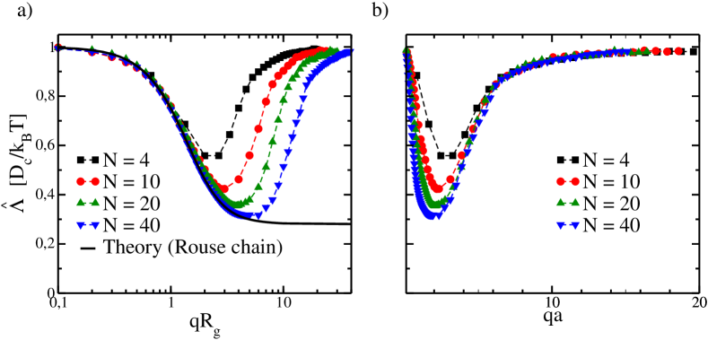
Figure 1: Rescaled mobility functions $\Lambda$ for polymer chains with different chain length as indicated. a) Logarithmic plot versus $qR_{{}_{G}}$. b) Linear plot versus $qa$, where $a$ is the statistical segment length. The black solid line shows the theoretical results from Ref. [57]

In CG polymer models, one represents polymers by relatively short, possibly very short chains. This turns out to have a significant impact on the mobility function. To investigate the chain length effects, we have carried computer simulations of spring-bead chains with harmonic bond potentials and different numbers of beads. Apart from being connected by bonds, monomers do not interact with each other. They move according to overdamped Brownian dynamics equations with a monomer friction constant $\zeta$. To determine the mobility functions from the simulation data, we first determine the single chain structure factor $g(\mathbf{q},t)$ from the simulation trajectories and then evaluate the integral $G(\mathbf{q})$ and finally $\hat{\Lambda}$ according to Eq. (2), applying an extrapolation procedure as described in Ref. [56] if necessary. The results for different chain lengths are presented in Fig. 1. To normalize the data, the mobilities are divided by the respective polymer diffusion constants $D_{c}=1/k_{{}_{B}}T\zeta N$. In Fig. 1 a), we also show the theoretical result for infinitely long Rouse polymers[57].

The simulation data agree well with the theory for small $q$. At larger $q$, however, they deviate. Different from Rouse polymers, the mobility functions of finite chains are nonmonotonic. They start from $\hat{\Lambda}(0)=D_{{}_{c}}/k_{{}_{B}}T$ and first decay, initially closely following the theoretical curve, but then assume a minimum and grow again, until they reach the original value, $\hat{\Lambda}(q)=D_{{}_{c}}/k_{{}_{B}}T$ at $q\to\infty$. In the small $q$ regime, the curves for different chain lengths collapse onto each other if plotted against $qR_{{}_{G}}$; in the large $q$ regime, they collapse if plotted as a function of $q$ only (made dimensionless by multiplying with the the statistical segment length $a$).

In the DDFT (Eq. (1)), the asymptotic large $q$ behavior of $\hat{\Lambda}$ describes that expected for a fluid of monomers which move independently with the diffusion constant $D_{0}=\hat{\Lambda}(\infty)N=1/k_{{}_{B}}T\zeta$[51, 59]. Hence, we observe a crossover from a collective ”chain mobility” to a ”monomer mobility” in chains with finite length $N$. The crossover point (the position of the minimum) scales roughly like $(qR_{{}_{G}})_{c}\sim N^{1/3}$ as a function of chain length. This seems to suggest that the crossover wavelength is determined by the average distance $d$ of monomers in the coil, which is set by the local density, $d\sim\rho^{1/3}$ with $\rho=N/R_{{}_{G}}^{3}$. In the limit of infinite chain length, the crossover point $(qR_{{}_{G}})_{c}$ moves to infinity. However, the value of the bare wavevector at the crossover, $(qa)_{c}$, moves to zero for infinite chain length.

The reason why the mobility of the finite chain at large $(qR_{{}_{G}})$ differs from that of the infinite chain can be rationalized as follows: In the regime $1\ll(qR_{{}_{G}})\ll(qR_{{}_{G}})_{c}$, the local mobility is dominated by the collective motion of whole chain portions with a locally scale invariant conformations. The effective friction of such a ”wad” is reduced, compared to that of a monomer, and can be calculated from its local self-similar structure[57]. On the other hand, on ultra-short length scales with $(qR_{{}_{G}})_{c}\ll(qR_{{}_{G}})$, the effect of chain connectivity becomes negligible and monomers diffuse individually. The two regimes (”wad” diffusion and monomer diffusion) are well separated in real polymer systems. However, in CG model systems of short chains, they move closer to each other and overlap.

When devising dynamic mapping schemes for such extremely CG polymers systems that cover kinetic processes, one is thus faced with a fundamental problem: It is impossible to accurately represent dynamic processes on both global and local (”wad”) length scales with simple time scale matching. If one uses the time scale of chain diffusion for time mapping, the time scales of local ordering, e.g., at interfaces, are overestimated by a factor of roughly 3.6. On the other hand, if maps the time scale of local ordering, the global chain diffusion is underestimated.

We should note that related finite chain length effects are also observed in the static structure factor, $g(\mathbf{q},0)$, although they are much less dramatic: For infinitely long chains, $1/Ng(\mathbf{q},0)$ drops from 1 (at $\mathbf{q}=0$) to zero at large $\mathbf{q}R_{{}_{G}}\to\infty$, whereas it levels off at $1/N$ for finite chains. In principle, this can be corrected by an appropriate backmapping procedure [60], i.e., restoring structure in the coarse-grained beads in retrospect. In the case of the dynamics, a different approach must be taken.

3 Adapting the CG polymer dynamics on multiple length scales

We will now propose a way to adjust the CG dynamics of in a CG polymer system such that it has the same mobility function than the target system of large polymers over the whole range of $\mathbf{q}$ vectors up to $(qR_{{}_{G}})_{c}$. The idea is slow down the internal modes, such that the CG monomers effectively have the mobility of a ”wad”, without changing the diffusion constant of the whole chains and the static structure of the chains. To this end, we have to introduce different friction constants for internal modes and global diffusion.

3.1 Method

We consider linear Gaussian chains of length $N$ with global chain friction $\gamma_{t}$. Our goal is to devise a modified dynamical model that allows for different internal friction constants while not affecting the static behavior of the chain. The diffusion constant of the whole chain will be kept fixed.

The monomer coordinates are given by $\mathbf{R}_{i}(t)$, and the total potential is given by $U[\{\mathbf{R}_{i}\}]$. Thus the force acting on monomer $i$ is given by $\mathbf{f}_{i}=-\nabla_{\mathbf{R}_{i}}U$. The center of mass of the chain is given by $\mathbf{R}_{t}(t)=\frac{1}{N}\sum_{i}\mathbf{R}_{i}$ and the total force acting on all monomers is $\mathbf{f}_{t}(t)=\sum_{i}\mathbf{f}_{i}(t)$.

3.1.1 Overdamped Brownian dynamics with two friction constants.

The simplest Ansatz is to introduce two friction constants, one for the center of mass motion of the chain and one for the relative motion with respect to the center of mass. We will illustrate this approach using the example of a overdamped Brownian dynamics. We introduce alternative coordinates $\mathbf{R}_{t}$ (center of mass) and $\mathbf{r}_{i}=\mathbf{R}_{i}-\mathbf{R}_{t}$ (internal coordinates), i.e., $\sum_{i}\mathbf{r}_{i}=0$. Rewriting the potential energy as a function of these coordinates, we obtain a new potential function

$$\tilde{U}[\mathbf{R}_{t},\{\mathbf{r}_{i}\}]=U[\{\mathbf{R}_{t}+\mathbf{r}_{i}\}].$$ (14)

To reproduce the identical static averages, the generalized forces $\tilde{\mathbf{f}}_{i}$ acting on coordinates $\mathbf{R}_{t}$, $\mathbf{r}_{i}$ are derived from $\tilde{U}$ with an additional Lagrange multiplier $\mathbf{\lambda}$ (a vector) that accounts for the constraint $\sum_{i}\mathbf{r}_{i}\equiv 0$:

$$\tilde{\mathbf{f}}_{t} = -\nabla_{\mathbf{R}_{t}}\tilde{U}=\sum_{i}(-\nabla_{\mathbf{R}_{i}}U)\frac{\partial\mathbf{R}_{i}}{\partial\mathbf{R}_{t}}=\sum_{i}\mathbf{f}_{i}=\mathbf{f}_{t}$$ (15)

$$\tilde{\mathbf{f}}_{i} = -\nabla_{\mathbf{r}_{i}}(\tilde{U}+\mathbf{\lambda}\cdot\sum_{i}\mathbf{r}_{i})=\mathbf{f}_{i}-\mathbf{\lambda}$$ (16)

The constraint forces must be chosen such that the constraint is fulfilled at all times. The dynamical equations are overdamped Langevin equations

$$\dot{\mathbf{R}}_{t} = \gamma_{t}\tilde{\mathbf{f}}_{t}+\mathbf{\xi}_{t}=\gamma_{t}\mathbf{f}_{t}+\xi_{t}$$ (17)

$$\dot{\mathbf{r}}_{i} = \gamma_{m}\tilde{\mathbf{f}}_{i}+\mathbf{\xi}_{i}=\gamma_{m}(\mathbf{f}_{i}-\mathbf{\lambda})+\mathbf{\xi}_{i}$$ (18)

with inverse friction constants $\gamma_{t}$ and $\gamma_{m}$. The value of $\gamma_{t}$ is chosen such that the chain has the desired diffusion constant. The value of $\gamma_{m}$ can be used for mapping the dynamics on short scales. The variables $\mathbf{\xi}_{t},\mathbf{\xi}_{i}$ describe uncorrelated Gaussian noise with mean zero ($\langle\xi_{\alpha}\rangle=0$) which satisfy the fluctuation-dissipation relation, i.e., $\langle\mathbf{\xi}_{t}(t)\mathbf{\xi}_{t}(t^{\prime})\rangle=2k_{{}_{B}}T\gamma_{t}\mathbf{1}\delta(t-t^{\prime})$, $\langle\mathbf{\xi}_{i}(t)\mathbf{\xi}_{i}(t^{\prime})\rangle=2k_{{}_{B}}T\gamma_{m}\mathbf{1}\delta(t-t^{\prime})$, and $\langle\mathbf{\xi}_{\alpha}(t)\mathbf{\xi}_{\beta}(t^{\prime})\rangle=0$ for $\alpha\neq\beta$. From the constraint $\sum_{i}\mathbf{r}_{i}\equiv 0$, we derive $\sum_{i}\dot{\mathbf{r}}_{i}\equiv 0$, which allows to express $\mathbf{\lambda}$ as $\mathbf{\lambda}=\frac{1}{N}(\mathbf{f}_{t}+\frac{1}{\gamma_{m}}\sum_{i}\mathbf{\xi}_{i})$, hence Eq. (18) reads

$$\dot{\mathbf{r}}_{i}=\gamma_{m}(\mathbf{f}_{i}-\frac{1}{N}\mathbf{f}_{t})+\mathbf{\xi}_{i}-\frac{1}{N}\sum_{j}\mathbf{\xi}_{j}.$$ (19)

This finally yields the modified equations of motion for monomers $\mathbf{R}_{i}$:

$$\dot{\mathbf{R}}_{i}=\gamma_{m}\mathbf{f}_{i}+\gamma_{t,\mbox{\tiny eff}}\mathbf{f}_{t}+\eta_{i}\quad\mbox{with}\quad\gamma_{t,\mbox{\tiny eff}}=\gamma_{t}-\frac{1}{N}\gamma_{m}$$ (20)

where $\eta_{i}=\mathbf{\xi}_{i}+(\mathbf{\xi}_{t}-\frac{1}{N}\sum_{j}\mathbf{\xi}_{j})$. Note that $\eta_{i}$ is again a correlated Gaussian distribution noise with correlation matrix $\langle\eta_{i}(t)\eta_{j}(t^{\prime})\rangle=2k_{{}_{B}}T\delta(t-t^{\prime})[\gamma_{m}\delta_{ij}+\gamma_{t,\mbox{\tiny eff}}]$. We recover the regular equations for linear Rouse polymers in the case $\gamma_{t}=\frac{1}{N}\gamma_{m}$.

3.1.2 Generalizations.

The above modifications can also be applied to regular Langevin dynamics (with inertia). For beads of mass $m$, we obtain the modified equation of motion

$$m\ddot{\mathbf{R}}_{i}=\mathbf{f}_{i}-\zeta_{m}\dot{\mathbf{R}}_{i}-\zeta_{t,\mbox{eff}}\dot{\mathbf{R}}_{t}+\mathbf{f}^{R}_{i}(t)$$ (21)

where $\zeta_{m}=\gamma_{m}^{-1}$, $\zeta_{t,\mbox{eff}}=\frac{1}{N}\gamma_{t}^{-1}-\gamma_{m}^{-1}$, and $\mathbf{f}^{R}_{i}(t)$ is a Gaussian distributed stochastic force with correlation matrix $\langle\mathbf{f}^{R}_{i}(t)\mathbf{f}^{R}_{j}(t)\rangle=2k_{{}_{B}}T\mathbf{1}\delta(t-t^{\prime})[\zeta_{m}\delta_{ij}+\frac{1}{N}\zeta_{t,\mbox{eff}}]$. As in Eq. (19), it can be implemented as a linear combination of uncorrelated random forces $\mathbf{f}^{R}_{i}=\theta_{i}+\frac{1}{N}(\theta_{t}-\sum_{j}\theta_{j})$ with $\langle\theta_{t}(t)\theta_{t}(t^{\prime})\rangle=2k_{{}_{B}}T\gamma_{t}^{-1}\mathbf{1}\delta(t-t^{\prime})$ and $\langle\theta_{i}(t)\theta_{j}(t^{\prime})\rangle=2k_{{}_{B}}T\zeta_{m}\mathbf{1}\delta(t-t^{\prime})$.

Extensions to modified dynamical models with more than one internal friction constants are straightforward. For future reference, we briefly describe the resulting equations for a hierarchical model with three friction constants. We separate the polymer into two blocks of equal length, A and B, such that the block A comprises monomers $\mathbf{R}_{i}$ with $i\in\{1,...,N/2\}:=S_{A}$ and the block B monomers $\mathbf{R}_{i}$ with $i\in\{N/2+1,...,N\}=:S_{B}$. We distinguish between the forces $\mathbf{f}_{i}$ acting on monomers $i$, the force $\mathbf{f}_{t}=\sum_{i}\mathbf{f}_{i}$ acting on the whole chain, and the forces $\mathbf{f}_{A,B}=\sum_{i\in S_{A,B}}\mathbf{f}_{i}$ acting on the individual blocks A and B. As generalized coordinates, we choose the center of mass $\mathbf{R}_{t}$ of the full chain, the center of masses $\mathbf{r}_{A,B}$ of the blocks relative to $\mathbf{R}_{t}$, and the coordinates $\mathbf{r}_{i}$ of monomers relative to $\mathbf{r}_{A,B}$. The motion of $\mathbf{R}_{t}$, $\mathbf{r}_{A,B}$, and $\mathbf{r}_{i}$ are associated with separate inverse friction constants $\gamma_{t},\gamma_{b}$, and $\gamma_{m}$. Following the same program as in the previous subsection, we obtain the following dynamical equations for monomers $i$ belonging to the block $\alpha(i)$ ($\alpha=A,B$) (overdamped regime):

$$\dot{\mathbf{R}}_{i}=\gamma_{m}\mathbf{f}_{i}+\gamma_{b,\mbox{\tiny eff}}\mathbf{f}_{\alpha(i)}+\gamma_{t,\mbox{\tiny eff}}\mathbf{f}_{t}+\eta_{i}$$ (22)

with $\gamma_{b,\mbox{\tiny eff}}=\gamma_{b}-\frac{2}{N}\gamma_{m}$, $\gamma_{t,\mbox{\tiny eff}}=\gamma_{t}=\frac{1}{2}\gamma_{b}$, where the Gaussian noise is correlated according to

$$\langle\eta_{i}(t)\eta_{j}(t^{\prime})\rangle=2k_{{}_{B}}T\delta(t-t^{\prime})\big{[}\gamma_{m}\delta_{ij}+\gamma_{b,\mbox{\tiny eff}}\delta_{\alpha(i),\alpha(j)}+\gamma_{t,\mbox{\tiny eff}}\big{]}.$$ (23)

As in the previous examples, it can again be conveniently calculated as a sum over uncorrelated Gaussian noise terms. Similar equations can be derived for other distributions of friction constants.

3.2 Results

To evaluate our proposed approach, we consider an extreme test case and attempt to map a Rouse polymer onto very short discrete Gaussian chains (length $N$). As a preliminary remark, we note that the asymptotic value of the mobility function $\hat{\Lambda}(q)$ in the limit $q\to\infty$ is bounded from below by the corresponding value for chains with frozen conformations, where the chains only move as a whole, i.e.[61, 59] $\hat{\Lambda}(q)_{\mbox{\tiny frozen}}=\frac{D_{c}}{k_{{}_{B}}T}\frac{1}{N}g(q,0)\stackrel{{\scriptstyle q\to\infty}}{{\to}}\frac{D_{c}}{k_{{}_{B}}T}N^{-1}$. In order to be able to implement the limiting behavior of $\hat{\Lambda}(q)$ for Rouse polymers given by Eq. (12), CG chains must thus have a minimum length of $N=4$. Hence we will evaluate CG systems of Gaussian tetramers. We employ modified dynamics with two friction constants as described in the previous section, Section 3.1.

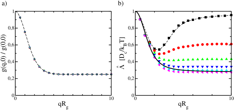
Figure 2: a) Normalized static structure factors $g(q,0)$ for chains with length $N=4$. Black dashed line shows the results from traditional overdamped Brownian dynamics simulations, the symbols those from modified dynamics approaches with two inverse friction constants $\gamma_{m}=N\gamma_{t},N\gamma_{t}/16$ and three inverse friction constants with two sets : ($\gamma_{b}=N\gamma_{t}/2,\gamma_{m}=N\gamma_{t}$) and ($\gamma_{b}=N\gamma_{t}/16,\gamma_{m}=N\gamma_{t}/16$). b) Rescaled mobility functions $\hat{\Lambda}(q)$ for the same chains from modified dynamics with two friction constants. For comparison the thin dashed line shows the results from traditional simulations, the thick solid line the theoretical results. For modified dynamics, the inverse relative monomer friction $\gamma_{m}$ is decreased from top to bottom: $\gamma_{m}=N\gamma_{t}$, $N\gamma_{t}/2$, $N\gamma_{t}/4$, $N\gamma_{t}/8$, $N\gamma_{t}/16$, $N\gamma_{t}/32$.

We first verify that the static behavior of the chain is not changed by the modified dynamics model. We characterize the static properties by the static structure factor, i.e., $g(q,t)$ at $t=0$. Fig. 2a) shows the static structure factors $g(q,0)$ for the polymer chains moving according to the modified dynamics approaches with two friction constants ($\gamma_{m}=N\gamma_{t},N\gamma_{t}/16$) and three friction constants (two sets: $\gamma_{b}=N\gamma_{t}/2,\gamma_{m}=N\gamma_{t}$ and $\gamma_{b}=N\gamma_{t}/16,\gamma_{m}=N\gamma_{t}/16$). The results from traditional overdamped Brownian simulations are shown as black solid curves for comparison. The agreement is excellent. Clearly the modified dynamics approaches do not change the static behavior of the chain.

Next we calculate the mobility function using the modified dynamics approach with two friction constants. Fig. 2b) shows the resulting mobility functions calculated for six values of inverse relative monomer friction ($\gamma_{m}=N\gamma_{t},N\gamma_{t}/2,N\gamma_{t}/4,N\gamma_{t}/8,N\gamma_{t}/16$, and $N\gamma_{t}/32$). The parameter $\gamma_{t}$, which sets the diffusion constant of the whole chain, is kept fixed. Additionally shown is the result from traditional simulations (black dashed line), and the theoretical results for Rouse polymers from our previous paper, Ref. [57] (black solid line).

At small $qR_{{}_{G}}$ ($qR_{{}_{G}}<2$), the relative monomer friction has no influence on the chain mobility functions. The data follow the theoretical curve for Rouse polymers. The overall translational motion of the chain dominates at small $qR_{{}_{G}}$. At intermediate and large $qR_{{}_{G}}$, the internal relaxation becomes important. If one decreases $\gamma_{m}$, the mobility function decreases. At $\gamma_{m}\approx N\gamma_{t}/16$, the data for the CG chain match those of the Rouse polymer. Hence, we can indeed obtain the target mobility function in modified dynamics simulations by tuning $\gamma_{m}$. This is the central message of the present paper.

However, the approach also has limitations. This becomes apparent when looking at the partial mobility functions for chain blocks, which is important for dynamical studies of block copolymer ordering and disordering[56, 57]. To illustrate this, we split our ultrashort chain ($N=4$) in two symmetric blocks A and B of length $N=2$ (see Sec. 3.1.2) and evaluate separately their mobility functions $\hat{\Lambda}_{AA}(q),\hat{\Lambda}_{BB}(q)$ as well as the cross-mobility $\hat{\Lambda}_{AB}(q)$. The same quantities can be calculated semi-analytically for Rouse polymers using the expressions given in our previous work, Ref. [57].

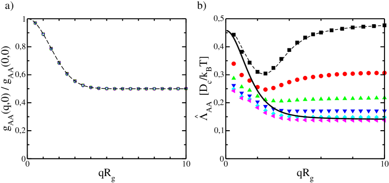
Figure 3: Same as Fig. 2, but now for the first half block (block A) of the chain. a) Normalized static structure factors $g(q,0)$, comparison of results from traditional dynamics (dashed line) and modified dynamics with different sets of inverse friction constants (symbols). b) Corresponding rescaled mobility function, comparison of results from traditional dynamics (dashed line), theory for Rouse polymers (thick solid line), and modified dynamics with inverse relative monomer friction, from top to bottom: $\gamma_{m}=N\gamma_{t}$, $N\gamma_{t}/2$, $N\gamma_{t}/4$, $N\gamma_{t}/8$, $N\gamma_{t}/16$, $N\gamma_{t}/32$.

The results are shown in Fig. 3. Note that $\hat{\Lambda}_{AA}(q)=\hat{\Lambda}_{BB}(q)$ due to symmetry and we also have $\hat{\Lambda}_{AB}(q)=\hat{\Lambda}_{BA}(q)$ and $\hat{\Lambda}(q)=\sum_{\alpha\beta}\hat{\Lambda}_{\alpha\beta}(q)$. Since $\hat{\Lambda}(q)$ is known from Fig. 2, it suffices to plot the data for $\hat{\Lambda}_{AA}(q)$ here. The same holds for the static structure factor $g_{\alpha\beta}(q)$. In Fig. 3a), we verify that the latter is not affected by the modified dynamics as expected. The data for the block mobility functions are given in Fig. 3b). At large $qR_{{}_{G}}$, if one decreases $\gamma_{m}$, the block mobility function decreases, and the target value (the value for Rouse polymers) can be matched for $\gamma_{m}=N\gamma_{t}/16$. Different from the total mobility function $\hat{\Lambda}$, however, the block mobility function $\hat{\Lambda}_{AA}$ is also affected by $\gamma_{m}$. In regular dynamics ($\gamma_{m}=\gamma_{t}N$), the behavior at small $qR_{{}_{G}}\to 0$ roughly matches that of short chains. However, if one reduces $\gamma_{m}$, it becomes smaller and deviates from the target. Hence it is not possible to match the kinetics of chain blocks on both short and long length scales in a CG model with such ultrashort chains, if one uses modified dynamics with two friction constants.

To analyze this in more detail, we inspect the structure of the block mobility functions. In Ref. [56], we have derived the following general expressions for $\hat{\Lambda}_{\alpha\beta}(q)$:

$$\hat{\Lambda}_{AA}(q)=\frac{1}{4k_{B}Tq^{2}N}\left(\frac{g(q,0)}{\tau_{R}}+\frac{\Delta(q,0)}{\tau_{\Delta}}\right)$$ (24)

$$\hat{\Lambda}_{AB}(q)=\frac{1}{4k_{B}Tq^{2}N}\left(\frac{g(q,0)}{\tau_{R}}-\frac{\Delta(q,0)}{\tau_{\Delta}}\right)$$ (25)

where $\tau_{R}=\frac{1}{g(q,0)}\int_{0}^{\infty}dtg(q,t)$, $\Delta(q,t)=g_{AA}(q,t)+g_{BB}(q,t)-g_{AB}(q,t)-g_{BA}(q,t)$, and $\tau_{\Delta}=\frac{1}{\Delta(q,0)}\int_{0}^{\infty}dt\Delta(q,t)$. Since $g(q,0)$ and $\Delta(q,0)$ are not affected by $\gamma_{m}$ (shown in Fig. 2a) and Fig. 3a)), the dependence of $\tau_{R}$ and $\tau_{\Delta}$ on $\gamma_{m}$ will determine the behavior of $\Lambda_{AA}$ and $\Lambda_{AB}$. The time scale $\tau_{R}$ characterizes the dynamics of the whole chain, and $\Delta$ characterizes the relaxation dynamics of blocks with respect to each other.

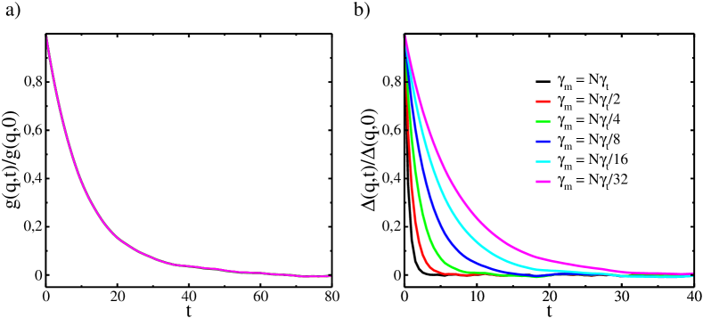
Figure 4: Normalized single chain dynamic structure factor (a) and $\Delta(q,t)$ (b) of polymer chain with length $N=4$ obtained from modified dynamics at $qR_{g}=0.5$. For both figures the monomer friction constants $\gamma_{m}$ is varied as $N\gamma_{t}$, $N\gamma_{t}/2$, $N\gamma_{t}/4$, $N\gamma_{t}/8$, $N\gamma_{t}/16$, $N\gamma_{t}/32$.

Here we focus on the small $qR_{{}_{G}}$ regime. Fig. 4 shows the normalized single chain dynamic structure factor $g(q,t)$ (a) and the quantity $\Delta(q,t)$ (b) of the CG chains as obtained from modified dynamics as a function of the simulation time $t$ at $qR_{{}_{G}}=0.5$. The inverse monomer friction $\gamma_{m}$ has practically no effect on the behavior of the single chain dynamic structure factor, hence the relaxation time $\tau_{R}$ does not change. For $\Delta(q,t)$, however, the relaxation slows down with decreasing $\gamma_{m}$, which results in an increase of $\tau_{\Delta}$. Combined with the equations above, we conclude that decreasing $\gamma_{m}$ will lead to a decrease in $\Lambda_{AA}$ and a increase in $\Lambda_{AB}$. The individual blocks relax more slowly and the two blocks move more cooperatively at small $qR_{{}_{G}}$ if the relative monomer friction is increased.

We have tested whether it is possible to decouple the motion of blocks at small $qR_{{}_{G}}$ by using a more versatile modified dynamics scheme with three friction constants. To this end, we have adopted the hierarchical model described in Sec. 3.1.2 and introduced an additional inverse block friction constant $\gamma_{b}$. Some representative results are shown in Fig. 5. The black line shows again the target mobility functions. In this example, we fix the inverse monomer friction parameter at a large value, $\gamma_{m}=N\gamma_{t}/16$, such that relative monomer motions are largely suppressed, and vary the inverse block friction constant $\gamma_{b}$ is varied. As can be seen from Fig. 5, introducing the hierarchical scheme with three friction constants does not improve the quality of the mapping. At the level of the block mobilities, the problems persist, and even the mapping of the total mobility function (Fig. 5a)) is not as good as in the system with two friction constants (Fig. 3). We have explored all possible parameter combinations of $\gamma_{b}$ and $\gamma_{m}$ and did not obtain any better results. Hence we conclude that dynamic mapping of block copolymers onto tetramers is not possible, and longer CG chains must be used to model such systems. Given that the chain length $N=4$ is the minimum chain length for homopolymer mapping as explained at the beginning of this section, it is perhaps not surprising that it is too small to map individual blocks.

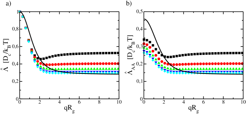
Figure 5: Mobility functions $\Lambda$ (a) and $\hat{\Lambda}_{AA}$ (b) for polymer chains with length $N=4$ from modified dynamics with three friction constants. The black solid line shows the target function, the mobility function for Rouse polymers. For modified dynamics, the inverse total friction constant $\gamma_{t}$ and the inverse relative monomer friction $\gamma_{m}=N\gamma_{t}/16$ are kept fixed, and the inverse block friction parameter $\gamma_{b}$ decreases from top to bottom: $N\gamma_{t}/2$, $N\gamma_{t}/4$, $N\gamma_{t}/8$, $N\gamma_{t}/16$, $N\gamma_{t}/32$.

4 Summary and Conclusion

To summarize, in this paper, we have presented a dynamic coarse-graining scheme for polymer systems with the goal of mapping the time scales of local kinetic processes over a large range of relevant length scales. The scheme builds on the single-chain mobility matrix, a wave-vector dependent integrated quantity that is derived from the single-chain structure factor. We have demonstrated that mobility functions can be used as sensitive diagnostic tools that highlight the quality of dynamic mapping schemes for polymers on different length scales. As an example, we have used them to evaluate extreme coarse-graining schemes that map long Rouse polymers onto CG chains with very few effective monomers, and shown that simple time scale matching fails for large wavevectors $q$. The reason is that in short chains, the motion of different monomers decouples for large $qR_{{}_{G}}$, whereas the dynamics remains cooperative in Rouse polymers. As a remedy, we have proposed a class of modified CG dynamics schemes where the relative motion of monomers is artificially slowed down, and shown that this can greatly improve the quality of dynamic mapping of homopolymers, even if the length of the CG chains is as short as $N=4$.

We have also investigated the limitations of the method. For homopolymers, we have established by analytical considerations that $N=4$ is the minimum CG chain length where consistent dynamic mapping is possible. In the case of block copolymers, this still seems too short and dynamic mapping of symmetric diblock copolymers onto tetramers was not possible. We found that slowing down the monomers increases the dynamic correlation between the different blocks in an undesired way, and it was not possible to find dynamical parameters that reproduce the mobility matrix function $\hat{\Lambda}_{\alpha\beta}(q)$ in a satisfactory manner over the whole range of $q$ vectors for CG chains with $N=4$. We conclude that dynamically consistent ”extreme” coarse-graining of block copolymers onto CG requires either further modifications or less extreme coarse-graining (i.e., larger $N$). When respecting these limitations, we believe that our scheme can have a wide range of interesting applications. We have tested it on linear Rouse polymers, but it can also be applied to polymers in other dynamic regimes, e.g., entangled polymers, and to other polymer architectures.

Our dynamic coarse-graining scheme is motivated by a Markovian approximation to the dynamics (Eq. (1)) that does not explicitly account for memory effects in polymer dynamics. Mapping strategies that target the full frequency dependent mobility matrix of the GLE, e.g., Eq. (10), should be even more accurate. However, it will likely not be possible to implement them without introducing frequency dependent mobility coefficients at the level of the CG model as well[34], which would greatly reduce the efficiency of CG simulations. On the other hand, CG simulations based on modified dynamics, e.g., Eqs. (20) or (21), are not much more expensive than regular CG simulations, as they neither require additional force evaluations, nor extra efforts (storage of data, auxiliary variables) to account for memory kernels[29]. The approach can additionally be motivated by the observation that polymer DDFTs based on the Markovian approximation – when using wave-vector dependent (i.e., nonlocal) mobility functions as in Eq. (1) – were found to reproduce kinetic processes in inhomogeneous polymer systems fairly accurately on time scales well below the Rouse time[56]. We have studied this for chains in the Rouse regime, corresponding investigations of other dynamical regimes are currently under way.

A large number of different internal friction constants can be introduced following the methods introduced in Section 3.1 and adjusted in order to optimally match the target mobility function. In the present work, we have mapped the parameters by straightforward trial and error. In the future, it will be desirable to develop more sophisticated iterative mapping schemes[62, 63, 64] and/or apply machine learning tools[31] to optimize the mapping. We believe that such developments will enable for dynamically accurate large scale simulations of kinetic processes in inhomogeneous polymer systems by use of extremely coarse-grained polymer models.

References

References

- [1] Utracki L A and Wilkie C A (eds) 2014 Polymer Blends Handbook 2nd ed (Springer)
- [2] Boudenne A, Ibos L, Candau Y and Thomas S (eds) 2011 Handbook of Multiphase Polymer Systems (Wiley)
- [3] Stamm M (ed) 2008 Polymer Surfaces and Interfaces 2nd ed (Springer)
- [4] McCrackin F l 1967 J. Chem. Phys. 47 1980
- [5] Baschnagel J, Binder K, Doruker P, Gusev A A, Hahn O, Kremer K, Mattice W, Müller-Plathe F, Murat M, Paul W, Santos S, Suter U W and Tries V 2000 Bridging the gap between atomistic and coarse-grained models of polymers: Status and perspectives Adv. Polymer Science: Viscoelasticity, atomistic models, statistical chemistry (Advances in Polymer Science vol 152) ed Abe, A (Springer) pp 41–156
- [6] Müller-Plathe F 2002 ChemPhysChem 3 754–769
- [7] Peter C and Kremer K 2009 Soft Matter 5 4357–4366
- [8] Peter C and Kremer K 2010 Faraday Discuss. 144(0) 9–24
- [9] Brini E, Algaer E A, Ganguly P, Li C, Rodríguez-Ropero F and van der Vegt N F A 2013 Soft Matter 9(7) 2108–2119
- [10] Noid W G 2013 J. Chem. Phys. 139 090901
- [11] Wagner J W, Dama J F, Durumeric A E P and Voth G A 2016 J. Chem. Phys. 145 044108
- [12] Doi M and Edwards S F 2013 The Theory of Polymer Dynamics (Oxford University Press)
- [13] Maier W and Saupe A 1959 Z. Naturforsch. 14a 882–889
- [14] Maier W and Saupe A 1960 Z. Naturforsch. 15a 287–292
- [15] de Gennes P G and Prost J 1995 The Physics of Liquid Crystals (Oxford University Press)
- [16] Olsen B D, Shah M, Ganesan V and Segalman R A 2008 Macromolecules 41 6809–6817
- [17] Greco C, Jiang Y, Chen J Z Y, Kremer K and Daoulas K C 2016 J. Chem. Phys. 145 184901
- [18] Martin J, Davidson E C, Greco C, Xu W, Bannock J H, Agirre A, de Mello J, Segalman R A, Stingelin N and Daoulas K C 2018 Chem. Mater. 30 748–761
- [19] Glaser J, Qin J, Medapuram P and Morse D C 2014 Macromolecules 47 851–869
- [20] Hannon A F, Sunday D F, Bowen A, Khaira G, Ren J, Nealey P F, de Pablo J J and Kline R J 2018 Mol. Syst. Design & Eng. 3 376–389
- [21] Beardsley T M and Matsen M W 2019 J. Chem. Phys. 150 174902
- [22] Tschöp W, Kremer K, Batoulis J, Bürger T and Hahn O 1998 Acta Polymerica 49 61–74
- [23] Tschöp W, Kremer K, Hahn O, Batoulis J and Bürger T 1998 Acta Polymerica 49 75–79
- [24] Zwanzig R 1961 Physical Review 124 983–992
- [25] Mori H 1965 Progress of Theoretical Physics 33 423–455
- [26] Zwanzig R 2001 Nonequilibrium statistical mechanics (New York: Oxford University Press)
- [27] Li Z, Bian X, Li X and Karniadakis G E 2015 J. Chem. Phys. 143 243128
- [28] Li Z, Bian X, Yang X and Karniadakis G E 2016 J. Chem. Phys. 145 044102
- [29] Li Z, Lee H S, Darve E and Karniadakis G E 2017 J. Chem. Phys. 146 014104
- [30] Wang S, Li Z and Pan W 2019 Soft matter 15 7567–7582
- [31] Wang S, Ma Z and Pan W 2020 Soft Matter 16(36) 8330–8344
- [32] Chen M, Li X and Liu C 2014 J. Chem. Phys. 141 064112
- [33] Ma L, Li X and Liu C 2016 J. Chem. Phys. 145 204117
- [34] Lee H S, Ahn S H and Darve E F 2019 J. Chem. Phys. 150 174113
- [35] Deichmann G and van der Vegt N F A 2018 J. Chem. Phys. 149 244114
- [36] Hijón C, Español P, Vanden-Eijnden E and Delgado-Buscalioni R 2010 Faraday Discuss. 144(0) 301–322
- [37] Laradji M, Guo H and Zuckermann M J 1994 Physical Review E 49 3199–3206
- [38] Soga K G, Guo H and Zuckermann M J 1995 Europhys. Lett. 29 531–536
- [39] Pagonabarraga I and Frenkel D 2001 J. Chem. Phys. 115 5015–5026
- [40] Daoulas K C and Müller M 2006 J. Chem. Phys. 125 184904
- [41] Pike P Q, Detcheverry F A, Müller M and de Pablo J 2009 J. Chem. Phys. 131 084903
- [42] Milano G and Kawakatsu T 2009 J. Chem. Phys. 130 214106
- [43] Müller M 2011 J. Stat. Phys. 145 967–1016
- [44] Daoulas K C, Rühle V and Kremer K 2012 J. Phys.-Condens. Mat. 24 284121
- [45] Sevink G, Charlaganov M and Fraaije J 2013 Soft Matter 9 2816–2831
- [46] Kawasaki K and Sekimoto K 1987 Physica A 143 349 – 413
- [47] Kawasaki K and Sekimoto K 1988 Physica A 148 361 – 413 ISSN 0378-4371
- [48] Fraaije J G E M 1993 J.Chem.Phys. 99 9202–9212
- [49] Fraaije J G E M, van Vlimmeren B A C, Maurits N M, Postma M, Evers O A, Hoffmann C, Altevogt P and Goldbeck-Wood G 1997 J.Chem.Phys. 106 4260–4269
- [50] Kawakatsu T, Doi M and Hasegawa R 1999 Int. J. Mod. Phys. C 10 1531–1540
- [51] Müller M and Schmid F 2005 Incorporating Fluctuations and Dynamics in Self-Consistent Field Theories for Polymer Blends (Berlin, Heidelberg: Springer Berlin Heidelberg) pp 1–58
- [52] te Vrugt M, Löwen H and Wittkowski R 2020 Adv. in Physics 69 121–247
- [53] Semenov A 1986 JETP 63 717–720
- [54] Wang G, Ren Y and Müller M 2019 Macromolecules 52 7704–7720
- [55] Rottler J and Müller M 2020 ACS Nano 14(10) 13986–13994
- [56] Mantha S, Qi S and Schmid F 2020 Macromolecules 53 3409–3423 ISSN 0024-9297
- [57] Schmid F and Li B 2020 Polymers 12 2205 ISSN 2073-4360
- [58] Ghasimakbari T and Morse D C 2019 Macromolecules 52 7762–7778
- [59] Qi S and Schmid F 2017 Macromolecules 50 9831–9845
- [60] Zhang G, Moreira L A, Stuehn T, Daoulas K C and Kremer K 2014 ACS Macro Lett. 3 198
- [61] Maurits N M and Fraaije J G E M 1997 J. Chem. Phys. 107 5879–5889
- [62] Jung G, Hanke M and Schmid F 2017 J. Chem. Theory Comp. 13 2481–2488
- [63] Jung G, Hanke M and Schmid F 2018 Soft matter 14 9368–9382
- [64] Meyer H, Pelagejcev P and Schilling T 2019 EPL (Europhysics Letters) 128 40001