Communication Near-Field Millimeter-Wave Imaging via Circular-Arc MIMO Arrays

Abstract

Millimeter-wave (MMW) imaging has a wide prospect in application of concealed weapons detection. We propose a circular-arc multiple-input multiple-output (MIMO) array scheme with uniformly spaced transmit and receive antennas along the horizontal-arc direction, while scanning along the vertical direction. The antenna beams of the circular-arc MIMO array can provide more uniform coverage of the imaging scene than those of the linear or planar MIMO arrays. Further, a near-field three-dimensional (3-D) imaging algorithm, based on the spatial frequency domain processing, is presented with analysis of sampling criteria and resolutions. Numerical simulations, as well as comparisons with the back-projection (BP) algorithm, are provided to show the efficacy of the proposed approach.

I Introduction

Millimeter-wave (MMW) imaging can provide high resolutions of the target under test. Thus, it is of interest in a wide applications, such as remote sensing [1], biomedical diagnosis [2], and indoor target tracking [3]. In recent years, there is an increasing demand for MMW to detect concealed weapons and contraband carried by personnel [4, 5, 6, 7], due to the fact that MMW can penetrate regular clothing to form an image of a person as well as the concealed objects with no health hazard at moderate power levels.

Usually, the antenna apertures are formed by 1-D monostatic arrays accompanied by mechanical scanning. The monostatic arrays need to satisfy the Nyquist sampling criterion, which leads to high number of antennas and switches. State-of-the-art MMW imaging systems employ multiple-input multiple-output (MIMO) arrays to reduce the number of elements [8, 6, 7]. Another merit of using MIMO lies in the fact that it can reduce the reconstructed artifacts induced by multipath reflections, which are prevalent in the monostatic array systems [5, 9, 10].

Imaging systems combining 1-D linear MIMO arrays and synthetic aperture radar (SAR) were discussed in [11, 12, 13, 14, 15] for concealed weapons detection. The two-dimensional (2-D) MIMO arrays with different topologies were studied in [16, 17, 7, 18, 19, 20] for near-field imaging. In so doing, the mechanical scanning is eliminated, which acheives real-time data acquisition. However, the cost and complexity of 2-D MIMO array systems are much higher than those constructed by a 1-D array with mechanical scanning perpendicular to the array dimension.

The 1-D ultrawideband (UWB) MIMO array was designed according to the effective aperture approach in [11] associated with a time-domain imaging algorithm. In [12], the 1-D linear MIMO arrays were optimized for short-range applications also on the basis of effective aperture approach. In [13], imaging algorithms based on the modified Kirchhoff method were derived for linear MIMO arrays with receivers evenly distributed. A spatial frequency domain imaging algorithm was developed in [14] for a linear MIMO array system associated with cylindrical scanning. The extended phase shift migration algorithm was studied in [15] for a MIMO-SAR system working at Terahertz band.

The aforementioned MIMO arrays are all configured with antennas placed on a straight line or a plane. Usually, two separate dense transmit subarrays were set at both ends of the undersampled receive array for the 1-D MIMO array design. This scheme can hardly provide an even illumination of a large imaging area along the array direction. A single-frequency MIMO-arc array based azimuth imaging method was presented in [21], based on the geometry transformation from the arc array to the equivalent linear array [22].

In this communication, we propose a circular-arc MIMO array based three-dimensional (3-D) imaging scheme. The transmit and receive antennas are evenly placed along the horizontal-arc direction. And the array is mechanically scanned along its perpendicular direction to obtain a cylindrical aperture, as illustrated in Fig. 1. The antenna beams of the circular-arc MIMO array cover the imaging area more evenly than those of the linear or planar MIMO arrays. Furthermore, we present a near-field 3-D imaging algorithm based on the spatial frequency domain processing, to fully utilize the fast Fourier transforms (FFTs), for the circular-arc MIMO array system. The key to obtain the imaging algorithm is to solve the convolution of the Green’s functions in the Fourier domain, which is, however, hard to be resolved. We solve it through using an approximation of the radial distances between antennas and target pixels in the cylindrical coordinates. Then, the spatial frequency domain imaging algorithm can be acquired based on the decomposition of the cylindrical waves into superposition of plane waves.

The rest of the communication is organized as follows: In the next section, we formulate the imaging algorithm based on solving the convolution of the Green’s functions in the spatial frequency domain. The sampling criteria and resolutions are outlined. Numerical results are shown in Section III. And concluding remarks follow at the end.

II Circular-Arc MIMO Array Based Imaging

II-A Imaging Algorithm

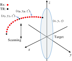
Figure 1: Topology of the circular-arc MIMO array based MMW imaging.

The circular-arc MIMO array based imaging geometry is shown in Fig. 1, where the transmit and receive antennas are uniformly spaced along a circular arc, meanwhile, scanning along the vertical direction. The demodulated scattered waves are given by,

$$s(k,\theta_{T},\theta_{R},z^{\prime})\!=\!\iiint\!\!g(x,y,z)e^{-\mathrm{j}k(R_{T}+R_{R})}\mathrm{d}x\mathrm{d}y\mathrm{d}z,$$ (1)

where $k=\frac{2\pi f}{c}$ denotes the wavenumber, $f$ is the working frequency, $c$ is the speed of light, $g(x,y,z)$ represents the scattering coefficient of the target located at $(x,y,z)$, $R_{T}$ and $R_{R}$ are the distances from the transmit antenna to the target and from the target to the receive antenna, respectively, which can be expressed as,

$$R_{T} =\sqrt{\rho_{T}^{2}+(z-z^{\prime})^{2}},$$

$$R_{R} =\sqrt{\rho_{R}^{2}+(z-z^{\prime})^{2}},$$

where

$$\rho_{T}=\sqrt{(x-R_{0}\sin\theta_{T})^{2}+(y+R_{0}\cos\theta_{T})^{2}},$$ (2)

$$\rho_{R}=\sqrt{(x-R_{0}\sin\theta_{R})^{2}+(y+R_{0}\cos\theta_{R})^{2}}.$$ (3)

The transmit and receive positions are denoted by $(R_{0},\theta_{T},z^{\prime})$ and $(R_{0},\theta_{R},z^{\prime})$, respectively, in the cylindrical coordinates, where $R_{0}$ represents the radius of the circular array.

Next, we derive a spatial frequency domain algorithm from this imaging scheme. Performing the Fourier transform on both sides of (1) with respect to $z^{\prime}$ and using the property of convolution in the Fourier domain, we have

$$s(k,\theta_{T},\theta_{R},k_{z^{\prime}})=\iiint g(x,y,z)\cdot$$ (4)

$$\mathcal{F}_{z^{\prime}}[e^{-\mathrm{j}kR_{T}}]\circledast_{k_{z^{\prime}}}\mathcal{F}_{z^{\prime}}[e^{-\mathrm{j}kR_{R}}]\mathrm{d}x\mathrm{d}y\mathrm{d}z.$$

The exponential terms $e^{-\mathrm{j}kR_{T}}$ and $e^{-\mathrm{j}kR_{R}}$ are referred to as the free space Green’s functions, whose Fourier transforms with respect to $z^{\prime}$ can be expressed as [23],

$$\mathcal{F}_{z^{\prime}}[e^{-\mathrm{j}kR_{T}}]=e^{-\mathrm{j}\sqrt{k^{2}-k^{2}_{z^{\prime}}}\rho_{T}}e^{-\mathrm{j}k_{z^{\prime}}z},$$ (5)

$$\mathcal{F}_{z^{\prime}}[e^{-\mathrm{j}kR_{R}}]=e^{-\mathrm{j}\sqrt{k^{2}-k^{2}_{z^{\prime}}}\rho_{R}}e^{-\mathrm{j}k_{z^{\prime}}z}.$$ (6)

Substituting (5) and (6) in (4), we obtain,

$$s(k,\theta_{T},\theta_{R},k_{z^{\prime}})=\iiint g(x,y,z)\cdot$$ (7)

$$[e^{-\mathrm{j}\sqrt{k^{2}-k^{2}_{z^{\prime}}}\rho_{T}}e^{-\mathrm{j}k_{z^{\prime}}z}\circledast_{k_{z^{\prime}}}e^{-\mathrm{j}\sqrt{k^{2}-k^{2}_{z^{\prime}}}\rho_{R}}e^{-\mathrm{j}k_{z^{\prime}}z}]\mathrm{d}x\mathrm{d}y\mathrm{d}z.$$

According to the form of convolution, (7) is rewritten as,

$$s(k,\theta_{T},\theta_{R},k_{z^{\prime}})=\iiint g(x,y,z)e^{-\mathrm{j}k_{z^{\prime}}z}\cdot$$ (8)

$$[e^{-\mathrm{j}\sqrt{k^{2}-k^{2}_{z^{\prime}}}\rho_{T}}\circledast_{k_{z^{\prime}}}e^{-\mathrm{j}\sqrt{k^{2}-k^{2}_{z^{\prime}}}\rho_{R}}]\mathrm{d}x\mathrm{d}y\mathrm{d}z.$$

However, it is hard to find the analytical solution of the convolution in the square brackets. In order to solve it, we approximate $\rho_{T}\approx\rho_{R}$ (denoted by $\rho_{0}$) temporarily, according to the geometry information between the imaging scene (mainly located around the axis of a cylindrical surface constructed by the mechanical scanned array) and the circular-arc MIMO array. Then, the convolution in the square brackets in (8) can be expressed as,

$$e^{-j\sqrt{k^{2}-k^{2}_{z^{\prime}}}\rho_{T}}\circledast_{k_{z^{\prime}}}e^{-j\sqrt{k^{2}-k^{2}_{z^{\prime}}}\rho_{R}}$$ (9)

$$\approx e^{-j\sqrt{k^{2}-k^{2}_{z^{\prime}}}\rho_{0}}\circledast_{k_{z^{\prime}}}e^{-j\sqrt{k^{2}-k^{2}_{z^{\prime}}}\rho_{0}}$$

$$=\int e^{-j\sqrt{k^{2}-\zeta^{2}}\rho_{0}}e^{-j\sqrt{k^{2}-(k_{z^{\prime}}-\zeta)^{2}}\rho_{0}}\mathrm{d}\zeta.$$

This integral can be calculated using the principle of stationary phase (POSP) [24]. Assuming

$$\vartheta(\zeta)=-\sqrt{k^{2}-\zeta^{2}}\rho_{0}-\sqrt{k^{2}-(k_{z^{\prime}}-\zeta)^{2}}\rho_{0},$$ (10)

then, using $\mathrm{d}\vartheta/\mathrm{d}\zeta=0$, we obtain $\zeta=k_{z^{\prime}}/2$. Thus, the convolution in (9) is given by,

$$e^{-j\sqrt{k^{2}-k^{2}_{z^{\prime}}}\rho_{T}}\circledast_{k_{z^{\prime}}}e^{-j\sqrt{k^{2}-k^{2}_{z^{\prime}}}\rho_{R}}\!\approx\!e^{j\vartheta(\zeta=k_{z^{\prime}}/2)}e^{-j\pi/4}$$ (11)

$$\approx e^{-j\sqrt{k^{2}-\frac{k_{z^{\prime}}^{2}}{4}}\rho_{T}}e^{-j\sqrt{k^{2}-\frac{k_{z^{\prime}}^{2}}{4}}\rho_{R}}e^{-j\pi/4}.$$

Note that we replace $\rho_{0}$ by the original $\rho_{T}$ and $\rho_{R}$ after the convolution. Here, we omit the envelope and the constant terms.

To evaluate the accuracy of (11), we show a numerical comparison between $e^{-j\sqrt{k^{2}-k^{2}_{z^{\prime}}}\rho_{T}}\circledast_{k_{z^{\prime}}}e^{-j\sqrt{k^{2}-k^{2}_{z^{\prime}}}\rho_{R}}$, which is calculated by the MATLAB function ‘conv’ as the accurate values, and $e^{-j\sqrt{k^{2}-{k_{z^{\prime}}^{2}}/{4}}\rho_{T}}e^{-j\sqrt{k^{2}-{k_{z^{\prime}}^{2}}/{4}}\rho_{R}}e^{-j\pi/4}$, under a configuration illustrated in Fig. 2 with parameters shown in Table I. The results are shown in Fig. 3. Clearly, the errors induced by the approximation $\rho_{T}\approx\rho_{R}$ are really small in the process of solving the convolution.

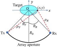
Figure 2: Geometry of a simple circular-arc MIMO array and target.

TABLE I: Parameters for Evaluating the Convolution

Parameters	Values
Radius of the circular array $(R_{0})$	1.0 m
working frequency	30 GHz
Angle of transmit antenna $\theta_{T}$	$-20^{\circ}$
Angle of receive antenna $\theta_{R}$	$20^{\circ}$
Scanning step along $z$ direction $\Delta z$	1 cm
Position of the considered target pixel $(x,y)$	$(0.25,0)$ (Unit: meter)

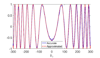
(a)

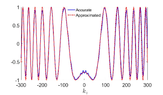
(b)

Figure 3: Comparison between the true convolution and the approximated one, (a) the real part, and (b) the imaginary part.

Substituting (11) in (8) yields,

$$s(k,\theta_{T},\theta_{R},k_{z^{\prime}})=\iiint g(x,y,z)e^{-{j}k_{z^{\prime}}z}\cdot$$ (12)

$$e^{-jk_{\rho}\rho_{T}}e^{-jk_{\rho}\rho_{R}}\mathrm{d}x\mathrm{d}y\mathrm{d}z,$$

where

$$k_{\rho}=\sqrt{k^{2}-k_{z^{\prime}}^{2}/4},$$ (13)

and $e^{-j\pi/4}$ is omitted. Based on (2) and (3), we decompose the cylindrical waves into a superposition of plane waves,

$$e^{-\mathrm{j}k_{\rho}\rho_{T}}=\int e^{-\mathrm{j}k_{x_{T}}(x-x_{T})}e^{-\mathrm{j}k_{y_{T}}(y-y_{T})}\mathrm{d}k_{x_{T}},$$ (14)

$$e^{-\mathrm{j}k_{\rho}\rho_{R}}=\int e^{-\mathrm{j}k_{x_{R}}(x-x_{R})}e^{-\mathrm{j}k_{y_{R}}(y-y_{R})}\mathrm{d}k_{x_{R}},$$ (15)

where $x_{T/R}=R_{0}\sin\theta_{T/R}$, $y_{T/R}=-R_{0}\cos\theta_{T/R}$, and $k_{x_{T/R}}^{2}+k_{y_{T/R}}^{2}=k_{\rho_{T/R}}^{2}$ with $k_{\rho_{T/R}}=k_{\rho}$. Here, the subscript ‘$T/R$’ denotes the transmit or receive parts for conciseness.

In order to achieve independent data with respect to $k_{\rho_{T}}$ and $k_{\rho_{R}}$, we perform dimension increase by dividing $k$ into two parts using the relation $k=k_{T}+k_{R}$, with

$$k_{\rho_{T}}=\sqrt{4k^{2}_{T}-k_{z^{\prime}}^{2}/4},$$ (16a)

$$k_{\rho_{R}}=\sqrt{4k^{2}_{R}-k_{z^{\prime}}^{2}/4}.$$ (16b)

To achieve this goal, we reformulate the data $s(k,\cdots)$ according to the illustration in Fig. 4. In so doing, we get a data matrix corresponding to the independent polar spatial frequency support $(k_{T},\theta_{T})$ and $(k_{R},\theta_{R})$, respectively.

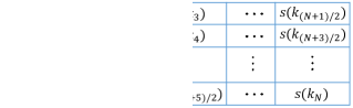
Figure 4: Dimension increasing from $s(k,\cdots)$ to $s(k_{T},k_{R},\cdots)$.

Then, substituting (14) and (15) in (12), and rearranging the integral sequence, we obtain,

$$s(k_{T},k_{R},\theta_{T},\theta_{R},k_{z^{\prime}})\!=\!\iint\!\iiint g(x,y,z)\cdot$$ (17)

$$e^{-\mathrm{j}(k_{x_{T}}+k_{x_{R}})x}e^{-\mathrm{j}(k_{y_{T}}+k_{y_{R}})y}e^{-\mathrm{j}k_{z^{\prime}}z}\cdot$$

$$e^{\mathrm{j}k_{x_{T}}x_{T}}e^{\mathrm{j}k_{y_{T}}y_{T}}e^{\mathrm{j}k_{x_{R}}x_{R}}e^{\mathrm{j}k_{y_{R}}y_{R}}\mathrm{d}x\mathrm{d}y\mathrm{d}z\mathrm{d}k_{x_{T}}\mathrm{d}k_{x_{R}}.$$

Clearly, the inner integrals over $x$, $y$, and $z$ can be expressed as a 3-D Fourier transform of $g(x,y,z)$ (denoted by $G(k_{x},k_{y},k_{z})$). Then, we have

$${s}(k_{T},k_{R}, \theta_{T},\theta_{R},k_{z})\!=\!\iint G(k_{x},k_{y},k_{z})\cdot$$ (18)

$$e^{\mathrm{j}k_{x_{T}}x_{T}}e^{\mathrm{j}k_{y_{T}}y_{T}}e^{\mathrm{j}k_{x_{R}}x_{R}}e^{\mathrm{j}k_{y_{R}}y_{R}}\mathrm{d}k_{x_{T}}\mathrm{d}k_{x_{R}},$$

where

$$k_{x}=k_{x_{T}}+k_{x_{R}},$$ (19a)

$$k_{y}=k_{y_{T}}+k_{y_{R}},$$ (19b)

$$k_{z}=k_{z^{\prime}}.$$ (19c)

The exponential terms associated with the integrals in the right side of (18) can be canceled in the cylindrical coordinates. The spatial frequency relations between the Cartesian and the cylindrical coordinates are given by,

$$k_{x_{T/R}}=k_{\rho_{T/R}}\sin\phi_{T/R},$$ (20a)

$$k_{y_{T/R}}=-k_{\rho_{T/R}}\cos\phi_{T/R}.$$ (20b)

The differential elements in (18) can then be approximated by $\mathrm{d}k_{x_{T}}\mathrm{d}k_{x_{R}}\approx k_{\rho_{T}}k_{\rho_{R}}\cos\phi_{T}\cos\phi_{R}\mathrm{d}\phi_{T}\mathrm{d}\phi_{R}$ due to the fact that $k_{\rho_{T}}$ and $k_{\rho_{R}}$ vary slowly along the direction of $k_{x_{T}}$ and $k_{x_{R}}$, respectively, for a limited angle extent subtended by the circular-arc array. Then, representing the spatial frequencies in the cylindrical coordinates, (18) is rewritten as

$${s}(k_{T},k_{R}, \theta_{T},\theta_{R},k_{z_{T}},k_{z_{R}})\!=\!k_{\rho_{T}}k_{\rho_{R}}\cdot$$ (21)

$$\!\iint\! G(k_{\rho_{T}},k_{\rho_{R}},\phi_{T},\phi_{R},k_{z})\cos\phi_{T}\cos\phi_{R}\cdot$$

$$e^{\mathrm{j}k_{\rho_{T}}R_{0}\cos(\theta_{T}-\phi_{T})}e^{\mathrm{j}k_{\rho_{R}}R_{0}\cos(\theta_{R}-\phi_{R})}\mathrm{d}\phi_{T}\mathrm{d}\phi_{R}.$$

Clearly, the integrals over $\phi_{T}$ and $\phi_{R}$ can be represented by the following convolutions with respect to $\theta_{T}$ and $\theta_{R}$, respectively.

$${s}( k_{T},k_{R},\theta_{T},\theta_{R},k_{z_{T}},k_{z_{R}})$$ (22)

$$= k_{\rho_{T}}k_{\rho_{R}}G(k_{\rho_{T}},k_{\rho_{R}},\theta_{T},\theta_{R},k_{z})\cos\theta_{T}\cos\theta_{R}\circledast_{T}$$

$$e^{\mathrm{j}k_{\rho_{T}}R_{0}\cos\theta_{T}}\circledast_{R}e^{\mathrm{j}k_{\rho_{R}}R_{0}\cos\theta_{R}},$$

where $\circledast_{T}$ and $\circledast_{R}$ denote convolutions in the $\theta_{T}$ and $\theta_{R}$ domains, respectively.

Note from (22) the scattering coefficients of target in the spatial frequency domain can be obtained through deconvolutions of the two exponential functions. We take the Fourier transforms of both sides of (22) with respect to $\theta_{T}$ and $\theta_{R}$, respectively. With the help of the Fourier property of convolution, we can write

$${{s}}(k_{T},k_{R},\xi_{T},\xi_{R},k_{z_{T}},k_{z_{R}})\!=\!k_{\rho_{T}}k_{\rho_{R}}\widetilde{G}(k_{\rho_{T}},k_{\rho_{R}},\xi_{T},\xi_{R},k_{z})\cdot$$ (23)

$$H^{(1)}_{\xi_{T}}(k_{\rho_{T}}R_{0})e^{\mathrm{j}\pi\xi_{T}/2}H^{(1)}_{\xi_{R}}(k_{\rho_{R}}R_{0})e^{\mathrm{j}\pi\xi_{R}/2},$$

where $\xi_{T/R}$ denotes the Fourier domain for $\theta_{T/R}$, $\widetilde{G}(\cdots)$ represents the Fourier transform of ${G(\cdots)}\cos\theta_{T}\cos\theta_{R}$ with respect to $\theta_{T}$ and $\theta_{R}$, and $H^{(1)}_{\xi_{T/R}}$ is the Hankel function of the first kind, $\xi_{T/R}$ order [23].

$$H^{(1)}_{\xi_{T/R}}(k_{\rho_{T/R}}R_{0})=\mathcal{F}_{\theta_{T/R}}[e^{\mathrm{j}k_{\rho_{T/R}}R_{0}\cos\theta_{T/R}}]e^{-\mathrm{j}\pi\xi_{T/R}/2}.$$ (24)

Thus, dividing both sides of (23) by the two Hankel functions and exponentials, and performing the inverse Fouirer transforms with respect to $\xi_{T}$ and $\xi_{R}$, we obtain

$$G(k_{\rho_{T}},k_{\rho_{R}},\theta_{T},\theta_{R},k_{z})=\frac{1}{k_{\rho_{T}}k_{\rho_{R}}\cos\theta_{T}\!\cos\theta_{R}}\cdot$$ (25)

$$\mathcal{F}^{-1}_{\xi_{T\!/\!R}}\!\!\Bigg{[}{\frac{{{s}}(k_{T},k_{R},\xi_{T},\xi_{R},k_{z_{T}},k_{z_{R}})e^{-\mathrm{j}\pi\xi_{T}/2}e^{-\mathrm{j}\pi\xi_{R}/2}}{H^{(1)}_{\xi_{T}}(k_{\rho_{T}}R_{0})H^{(1)}_{\xi_{R}}(k_{\rho_{R}}R_{0})}}\Bigg{]}.$$

Finally, interpolations based on (20a) and (20b) and dimension reduction [7] are implemented to change $G(k_{\rho_{T}},k_{\rho_{R}},\theta_{T},\theta_{R},k_{z})$ into $G(k_{x},k_{y},k_{z})$, over which the 3-D inverse FFT is performed to obtain $g(x,y,z)$.

II-B Sampling criteria

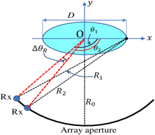
Figure 5: Illustration of the sampling criterion of circular-arc MIMO array.

We assume that the transmit array is undersampled, and the receive array is fully sampled. First, the requirement for the inter-element spacing of the receive array is considered. To avoid aliasing, the phase difference between two neighboring receive antennas has to be less than $\pi$ rad [7]. Considering the illustration in Fig. 5, we have $k(R_{1}-R_{2})\leq\pi$, where $R_{1}=\sqrt{R_{0}^{2}+\frac{D^{2}}{4}-R_{0}D\cos\theta_{1}}\approx R_{0}-\frac{D\cos\theta_{1}}{2}$, $R_{2}=\sqrt{R_{0}^{2}+\frac{D^{2}}{4}-R_{0}D\cos\theta_{2}}\approx R_{0}-\frac{D\cos\theta_{2}}{2}$, and $\theta_{1}=\theta_{2}+\Delta\theta_{R}$. Thus,

$$k(R_{1}-R_{2})$$

$$\approx k\frac{D\sin\theta_{2}\sin\Delta\theta_{R}}{2}\leq k\frac{D\sin\Delta\theta_{R}}{2}\approx k\frac{D\Delta\theta_{R}}{2}\leq\pi,$$

due to $\cos\Delta\theta_{R}\approx 1$ and $\sin\Delta\theta_{R}\approx\Delta\theta_{R}$ with a small inter-element spacing $\Delta\theta_{R}$ of the receive array. Then, we obtain

$$\Delta\theta_{R}\leq\frac{\lambda_{\text{min}}}{D},$$ (26)

where $\lambda_{\text{min}}$ denotes the minimum wavelength of the working EM waves, and $D$ is the maximum dimension along $x$ direction.

For the undersampled transmit array, there is no limit to the inter-element spacing as long as two antennas at least are put at the both ends of the receive array to ensure a comparable resolution with a monostatic array. Fig. 6 shows a comparison of 1-D imaging results obtained using a monostatic array with 61 transmit and 61 receive antennas as a benchmark, and using circular MIMO arrays with $N_{t}$ transmit antennas and 31 receive antennas. Note that the resolutions of MIMO arrays are slightly worse than that of the monostatic array due to the convolution in (22), which is equivalent to adding a weighting function (shaped like a triangle) to the spatial frequency data. On the other hand, the weighting function with respect to $N_{t}=2$ is shaped somewhat like a ‘U’-shape, which results in a slightly narrower main lobe but higher sidelobes than those of the other cases (such as $N_{t}=3$ or $31$). However, on the whole, the results in Fig. 6 have comparable resolutions.

As for the requirement for the mechanical scanning step along the vertical direction, according to $e^{-\text{j}k_{z}z^{\prime}}$ in (17), the scanning step should satisfy $k_{z_{\text{max}}}\Delta z^{\prime}\leq\pi$ to avoid aliasing effects. Based on (13), we have $k_{z_{\text{max}}}=2k_{\text{max}}\sin\frac{\Theta_{z}}{2}$, then,

$$\Delta z^{\prime}\leq\frac{\lambda_{\text{min}}}{4\sin\frac{\Theta_{z}}{2}},$$ (27)

where $\Theta_{z}$ denotes the minimum one between the antenna beamwidth and the angle subtended by the scanning length from the center of imaging scene.

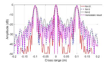
Figure 6: 1-D images along the horizontal direction by using circular-arc MIMO arrays with $N_{t}$ transmit antennas and 31 receive antennas, and by using a monostatic array with 61 transmit-receive pairs.

II-C Resolutions

First, consider the cross-range resolution along the direction of the circular-arc array. Note that the cross-range resolution is determined by the extent of the corresponding spatial frequency, which leads to,

$$\delta x=\frac{\pi}{k_{x_{\text{max}}}},$$ (28)

based on the exponential function $\exp(-\mathrm{j}k_{x}x)$, where $k_{x_{\text{max}}}$ denotes the maximum of $k_{x}$.

According to (19a), and the array configuration in Fig. 1, we note that $k_{x_{\text{max}}}=k_{x_{T_{\text{max}}}}+k_{x_{R_{\text{max}}}}$ with $k_{x_{T_{\text{max}}}}=k_{x_{R_{\text{max}}}}\approx k_{c}\sin(\Theta_{h}/2)$ with the help of (16a), (16b), and (20a), where $k_{c}$ denotes the center wavenumber of the working waves, and $\Theta_{h}$ represents the angle subtended by the array aperture, assuming that the beamwidth of each antenna can fully illuminate the target in the horizontal direction. Thus,

$$\delta x=\frac{\pi}{2k_{c}\sin\frac{\Theta_{h}}{2}}=\frac{\lambda_{c}}{4\sin\frac{\Theta_{h}}{2}}.$$ (29)

This is the same with that of the monostatic imaging scenario, which has been verified by the results in Fig. 6.

Similarly, the resolution along the $z$ direction is given by,

$$\delta z=\frac{\pi}{k_{z_{\text{max}}}}=\frac{\lambda_{c}}{4\sin\frac{\Theta_{z}}{2}},$$ (30)

where $\Theta_{z}$ denotes the minimal one between the angle subtended by the scanning length and the beamwidth of the antenna element.

Finally, the down-range resolution can be expressed as $\delta y=\frac{c}{2B}$, where $B$ denotes the bandwidth of the working EM waves.

III Results

TABLE II: Simulation Parameters

Parameters	Values
Radius of the circular array $(R_{0})$	1.0 m
Start frequency	30 GHz
Stop frequency	35 GHz
Number of frequency steps	25
Number of transmit antennas	5
Number of receive antennas	41
Interval of transmit antennas along circumference	9.9 cm
Interval of receive antennas along circumference	0.99 cm
Scanning step along elevation	1.0 cm

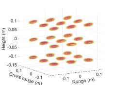
(a)

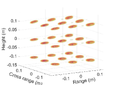
(b)

Figure 7: 3-D imaging results by (a) the proposed algorithm, and (b) BP, with a dynamic range of 20 dB.

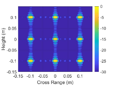
(a)

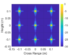
(b)

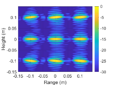
(c)

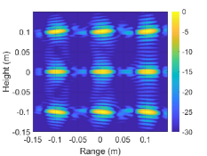
(d)

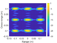
(e)

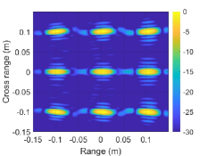
(f)

Figure 8: 2-D images with respect to the three coordinate planes by the proposed algorithm: (a), (c), (e); and by BP: (b), (d), and (f).

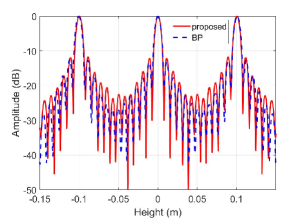
(a)

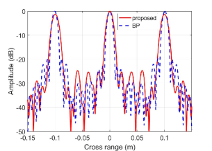
(b)

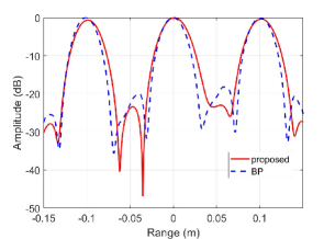
(c)

Figure 9: 1-D images corresponding to the (a) height, (b) horizontal, and (c) range dimensions, respectively.

In this section, we show more results of the proposed method in comparison with BP. The parameters for simulations are presented in Table II.

First, we provide simulations of point targets to compare focusing property with the BP algorithm. The 3-D imaging results are shown in Fig. 7. To view the details, the 2-D images with respect to the three coordinate planes are demonstrated in Fig. 8. Clearly, the results of the proposed algorithm have similar performance with those of BP. Fig. 9 shows the 1-D images where the main lobes and sidelobes of the point targets can be clearly demonstrated. Note that the resolutions along the horizontal cross-range and down-range directions in Figs. 9(c) and 9(d), respectively, of the proposed algorithm are slightly worse than those of BP, probably due to the information loss caused by the transformation from the polar to Cartesian grids.

Finally, we provide the results by using FEKO - a computational electromagnetics software [25], to simulate the scattered EM waves. The reconstructed images by the proposed algorithm and BP are shown in Figs. 10(a) and 10(b), respectively. Note that the focusing performance of the proposed algorithm is very close to that of BP, indicating further the effectiveness of the approach.

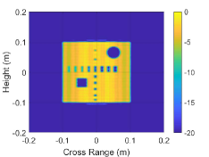
(a)

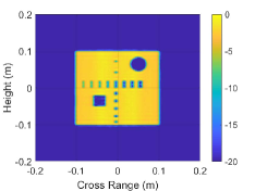
(b)

Figure 10: Imaging results by (a) the proposed algorithm, and (b) BP.

IV Conclusions

The paper presented a near-field 3-D MMW imaging scheme based on a circular-arc MIMO array associated with mechanical scanning along its perpendicular direction. The transmit and receive antennas are uniformly distributed over an arc of a circle. The circular-arc MIMO array can provide more even illuminations of the imaging area than the linear or planar MIMO arrays, which may offer better observation of the human body and any concealed items. Further, the imaging algorithm was presented based on the spatial frequency domain processing. Numerical experiments demonstrated the efficacy of the proposed imaging technique.

References

- [1] A. Moreira, P. Prats-Iraola, M. Younis, G. Krieger, and etc., “A tutorial on synthetic aperture radar,” IEEE Geosci. Remote Sens. Mag., vol. 1, pp. 6–43, March 2013.
- [2] S. Di Meo, P. F. Espín-López, A. Martellosio, and etc., “On the feasibility of breast cancer imaging systems at millimeter-waves frequencies,” IEEE Trans. Microw. Theory Tech., vol. 65, pp. 1795–1806, May 2017.
- [3] M. Amin, Through-the-Wall Radar Imaging. Taylor & Francis, 2010.
- [4] D. M. Sheen, D. L. McMakin, and T. E. Hall, “Near field imaging at microwave and millimeter wave frequencies,” in 2007 IEEE/MTT-S International Microwave Symposium, pp. 1693–1696, June 2007.
- [5] D. M. Sheen, D. L. McMakin, and T. E. Hall, “Three-dimensional millimeter-wave imaging for concealed weapon detection,” IEEE Trans. Microw. Theory Tech., vol. 49, pp. 1581–1592, Sep. 2001.
- [6] S. S. Ahmed, A. Schiessl, F. Gumbmann, M. Tiebout, S. Methfessel, and L. Schmidt, “Advanced microwave imaging,” IEEE Microw. Mag., vol. 13, no. 6, pp. 26–43, 2012.
- [7] X. Zhuge and A. G. Yarovoy, “Three-dimensional near-field MIMO array imaging using range migration techniques,” IEEE Trans. Image Process., vol. 21, pp. 3026–3033, June 2012.
- [8] Y. Álvarez, Y. Rodriguez-Vaqueiro, B. Gonzalez-Valdes, and etc., “Fourier-based imaging for subsampled multistatic arrays,” IEEE Trans. Antennas Propag., vol. 64, no. 6, pp. 2557–2562, 2016.
- [9] G. Gennarelli and F. Soldovieri, “Multipath ghosts in radar imaging: Physical insight and mitigation strategies,” IEEE J. Sel. Topics Appl. Earth Observations Remote Sens., vol. 8, no. 3, pp. 1078–1086, 2015.
- [10] Y. Álvarez, Y. Rodriguez-Vaqueiro, B. Gonzalez-Valdes, and etc., “Fourier-based imaging for multistatic radar systems,” IEEE Trans. Microw. Theory Tech., vol. 62, no. 8, pp. 1798–1810, 2014.
- [11] X. Zhuge and A. G. Yarovoy, “A sparse aperture MIMO-SAR-based UWB imaging system for concealed weapon detection,” IEEE Trans. Geosci. Remote Sens., vol. 49, pp. 509–518, Jan 2011.
- [12] F. Gumbmann and L. Schmidt, “Millimeter-wave imaging with optimized sparse periodic array for short-range applications,” IEEE Trans. Geosci. Remote Sens., vol. 49, pp. 3629–3638, Oct 2011.
- [13] J. Gao, Y. Qin, B. Deng, and etc., “Novel efficient 3D short-range imaging algorithms for a scanning 1D-MIMO array,” IEEE Trans. Image Process., vol. 27, pp. 3631–3643, July 2018.
- [14] J. Gao, B. Deng, Y. Qin, and etc., “An efficient algorithm for MIMO cylindrical millimeter-wave holographic 3-D imaging,” IEEE Trans. Microw. Theory Tech., vol. 66, pp. 5065–5074, Nov 2018.
- [15] H. Gao, C. Li, S. Wu, and etc., “Study of the extended phase shift migration for three-dimensional MIMO-SAR imaging in terahertz band,” IEEE Access, vol. 8, pp. 24773–24783, 2020.
- [16] S. S. Ahmed, A. Schiessl, and L. Schmidt, “A novel fully electronic active real-time imager based on a planar multistatic sparse array,” IEEE Trans. Microw. Theory Tech., vol. 59, pp. 3567–3576, Dec 2011.
- [17] X. Zhuge and A. G. Yarovoy, “Study on two-dimensional sparse MIMO UWB arrays for high resolution near-field imaging,” IEEE Trans. Antennas Propag., vol. 60, pp. 4173–4182, Sep. 2012.
- [18] K. Tan, S. Wu, Y. Wang, S. Ye, and etc., “A novel two-dimensional sparse MIMO array topology for UWB short-range imaging,” IEEE Antennas Wireless Propag. Lett., vol. 15, pp. 702–705, 2016.
- [19] K. Tan, S. Wu, Y. Wang, S. Ye, J. Chen, X. Liu, G. Fang, and S. Yan, “On sparse MIMO planar array topology optimization for UWB near-field high-resolution imaging,” IEEE Trans. Antennas Propag., vol. 65, no. 2, pp. 989–994, 2017.
- [20] J. Wang, P. Aubry, and A. Yarovoy, “3-D short-range imaging with irregular MIMO arrays using NUFFT-based range migration algorithm,” IEEE Trans. Geosci. Remote Sens., vol. 58, no. 7, pp. 4730–4742, 2020.
- [21] S. Wu, H. Wang, C. Li, and etc., “A modified omega-k algorithm for near-field single-frequency MIMO-arc-array-based azimuth imaging,” IEEE Trans. Antennas Propag., pp. 1–1, 2021.
- [22] Z. D. Qin, J. Ylitalo, and J. Oksman, “Circular-array ultrasound holography imaging using the linear-array approach,” IEEE Trans. Ultrason. Ferroelectr. Freq. Control, vol. 36, no. 5, pp. 485–493, 1989.
- [23] M. Soumekh, “Reconnaissance with slant plane circular SAR imaging,” IEEE Trans. Image Process., vol. 5, no. 8, pp. 1252–1265, 1996.
- [24] I. Cumming and F. Wong, Digital Processing of Synthetic Aperture Radar Data: Algorithms and Implementation. Artech House, 2005.
- [25] Altair Feko, Altair Engineering, Inc., www.altairhyperworks.com/feko.