Perturbative treatment of three-nucleon force contact terms in three-nucleon Faddeev equations

Abstract

We present a perturbative approach to solving the three-nucleon continuum Faddeev equation. This approach is particularly well suited to dealing with variable strengths of contact terms in a chiral three-nucleon force. We use examples of observables in the elastic nucleon-deuteron scattering as well as in the deuteron breakup reaction to demonstrate high precision of the proposed procedure and its capability to reproduce exact results. A significant reduction of computer time achieved by the perturbative approach in comparison to exact treatment makes this approach valuable for fine-tuning of the three-nucleon Hamiltonian parameters.

Special Issue: “Celebrating 30 years of Steven Weinberg’s papers on Nuclear Forces from Chiral Lagrangians”

1 Introduction

The nuclear force problem is the basic one for understanding nuclear phenomena. Since the birth of nuclear physics it has been at the centre of experimental and theoretical studies. Extensive efforts based on purely phenomenological approaches or incorporating the meson-exchange picture have led to numerous nucleon-nucleon (NN) potentials, able to describe with high precision a vast amount of available data mach_anp . In spite of the enormous progress in understanding properties of the two-nucleon interaction, applications of these ideas to the many-nucleon forces encountered consistency problems and called for a more systematic framework. The advent of QCD gave a new impetus to the derivation of nuclear forces and a major breakthrough occurred with the emergence of the effective field theory (EFT) concept and publishing of S. Weinberg’s seminal paper weinberg . It paved the way for developing accurate and precise nuclear forces within the EFT framework vankolck ; epel_nn_n3lo ; epel6a ; Epelbaum:2008ga ; machl6b .

The progress in constructing nuclear forces within EFT approach is presently documented by availability of numerous high precision NN potentials which provide satisfactory description of NN data in a wide energy range. Recently a new generation of chiral NN potentials was introduced and developed up to the fifth order (N⁴LO) of chiral expansion by the Bochum-Bonn epel1 ; epel2 and Idaho-Salamanca entem2017 groups. While in the Idaho-Salamanca force the nonlocal momentum space regularization is applied directly in momentum space by introducing a cutoff parameter $\Lambda$, the one-pion and two-pion exchange contributions in the Bochum-Bonn potential are regularized in coordinate space using a cutoff parameter $R$ and then transformed to momentum space. For the contact interactions the Bochum-Bonn NN force employs a simple Gaussian nonlocal momentum-space regulator with the cutoff $\Lambda=2R^{-1}$. Potentials of both groups are available for a number of regularization parameters. They provide a very good description of the NN data set (Idaho-Salamanca) or the phase shifts and mixing angles of the Nijmegen partial wave analysis nijmpwa (Bochum-Bonn), used to fix the low-energy constants accompanying the NN contact interactions. The latest and most precise EFT-based NN interaction is the so called semilocal momentum-space (SMS) regularized chiral potential of the Bochum-Bonn group preinert , developed up to N⁴LO and even including some terms from the next order of chiral expansion (N⁴LO⁺). In this potential a new momentum-space regularization scheme has been employed for the long-range contributions and a nonlocal Gaussian regulator has been applied to the minimal set of independent contact interactions. This new approach can be straightforwardly utilised to regularize also three-nucleon (3N) forces. That new family of semilocal chiral potentials provides an outstanding description of the NN data and is available up to N⁴LO⁺ for five values of the cutoff $\Lambda$.

Applications of EFT approach in the form of chiral perturbation theory (ChPT) have resulted not only in the theoretically well grounded NN potentials but also for the first time have given a possibility to apply in practical calculations NN forces augmented with consistent 3N interactions, both derived within the same formalism. Understanding of nuclear spectra and reactions based on these consistent chiral two- and many-body forces has become a hot topic of present day few-body studies and is also the main aim of the Low Energy Nuclear Physics International Collaboration (LENPIC) epel2019 .

The first nonvanishing contributions to the 3N force (3NF) appear at next-to-next-to-leading order of chiral expansion (N²LO) vankolck ; epel2002 and comprise in addition to the $2\pi$-exchange term two contact contributions with strength parameters $c_{D}$ and $c_{E}$ epel_tower . The difficult task to derive the chiral 3NF at next-to-next-to-next-to-leading order (N³LO) has been performed in 3nf_n3lo_long ; 3nf_n3lo_short . At that order five different topologies contribute to 3NF. Three of them are of long-range character 3nf_n3lo_long and are given by two-pion ($2\pi$) exchange graphs, by two-pion-one-pion ($2\pi-1\pi$) exchange graphs, and by the so-called ring diagrams. They are supplemented by the short-range two-pion-exchange-contact ($2\pi$-contact) term and by the leading relativistic corrections to 3NF 3nf_n3lo_short . The 3NF at N³LO order does not involve any new unknown low-energy constants (LECs) and depends only on two parameters, $c_{D}$ and $c_{E}$ that parameterize the leading one-pion-contact term and the 3N contact term present already at N²LO. The $c_{D}$ and $c_{E}$ values need to be then fixed at this order, as at N²LO, from a fit to few-nucleon data. At the higher order, N⁴LO, in addition to long- and intermediate-range interactions generated by pion-exchange diagrams krebs2012 ; krebs2013 , the chiral N⁴LO 3NF involves thirteen purely short-range operators, which have been worked out in girlanda2011 .

Since the advent of numerically exact three-nucleon continuum Faddeev calculations the elastic nucleon-deuteron (Nd) scattering and the deuteron breakup reaction have become a powerful tool to test modern models of the nuclear forces glo96 ; pisa ; hanover . With the appearance of high precision (semi)phenomenological NN potentials and first models of 3NF the question about the importance of 3NF has developed into the main topic of 3N system studies. That issue has been given a new impetus by ChPT-based approaches and the possibility to apply consistent two- and many-body nuclear forces, derived within this framework, in 3N continuum calculations.

First applications of (semi)phenomenological NN and 3N forces to elastic Nd scattering and to the nucleon-induced deuteron breakup reaction revealed interesting cases of discrepancies between pure two-nucleon (2N) theory and data, indicating possibly large 3NF effects wit2001 ; kuros2002 .

Using chiral 3NF’s in 3N continuum requires numerous time consuming computations with varying strengths of the contact terms in order to establish their values. They can be determined for example from the ³H binding energy and the minimum of the elastic Nd scattering differential cross section at the energy ($E_{lab}\approx 70$ MeV), where the effects of 3NF start to emerge in elastic Nd scattering wit2001 ; wit98 . Specifically at N²LO, after establishing the so-called ($c_{D},c_{E}$) correlation line, which for a particular chiral NN potential combined with a N²LO 3NF gives pairs of ($c_{D},c_{E}$) values reproducing the ³H binding energy, a fit to experimental data for the elastic Nd cross section is performed to determine the $c_{D}$ and $c_{E}$ strengths. Fine-tuning of the 3N Hamiltonian parameters requires an extensive analysis of available 3N elastic Nd scattering and breakup data. That ambitious goal calls for a significant reduction of computer time necessary to solve the 3N Faddeev equations. Thus finding an efficient emulator for exact solutions of the 3N Faddeev equations seems to be essential and of high priority.

In this paper we propose such an emulator and test its efficiency as well as ability to accurately reproduce exact solutions of 3N Faddeev equations. In Sec. 2 we briefly describe the formalism of 3N continuum Faddeev calculations and present the new scheme which is well-suited to fast calculations with varying strengths of the contact terms in a chiral 3NF. Tests and an evaluation of that new approach based on example observables in elastic Nd scattering and in selected breakup configurations are presented in Sec.  3. We summarize and conclude in Sec.  4.

2 Perturbative treatment of contact terms in 3N Faddeev equations

Theoretical predictions shown in the present paper were obtained within the 3N Faddeev formalism using chiral two- and three-body forces. The formalism itself and numerical performance were presented in numerous publications so we only briefly summarize the formalism and for details refer to  glo96 ; wit88 ; hub97 ; book .

Neutron-deuteron scattering with nucleons interacting via NN interactions $v_{NN}$ and a 3NF $V_{123}=V^{(1)}+V^{(2)}+V^{(3)}$, is described in terms of a breakup operator $T$ satisfying the Faddeev-type integral equation glo96 ; wit88 ; hub97

$$T|\phi\rangle = tP|\phi\rangle+(1+tG_{0})V^{(1)}(1+P)|\phi\rangle+tPG_{0}T|\phi\rangle$$ (1)

$$+ (1+tG_{0})V^{(1)}(1+P)G_{0}T|\phi\rangle\,.$$ (2)

The 2N $t$-matrix $t$ is the solution of the Lippmann-Schwinger equation with the interaction $v_{NN}$. $V^{(1)}$ is the part of a 3NF which is symmetric under the interchange of nucleons $2$ and $3$: $V_{123}=V^{(1)}(1+P)$. The permutation operator $P=P_{12}P_{23}+P_{13}P_{23}$ is given in terms of the transposition operators, $P_{ij}$, which interchange nucleons $i$ and $j$. The initial state $|\phi\rangle=|\mathbf{q}_{0}\rangle|\phi_{d}\rangle$ describes the free motion of the neutron and the deuteron with the relative momentum $\mathbf{q}_{0}$ and contains the internal deuteron wave function $|\phi_{d}\rangle$. Finally, $G_{0}$ is the resolvent of the three-body center-of-mass kinetic energy. The amplitude for elastic scattering leading to the two-body final state $|\phi^{\prime}\rangle$ is then given by glo96 ; hub97

$$\langle\phi^{\prime}|U|\phi\rangle = \langle\phi^{\prime}|PG_{0}^{-1}|\phi\rangle+\langle\phi^{\prime}|PT|\phi\rangle+\langle\phi^{\prime}|V^{(1)}(1+P)|\phi\rangle$$ (3)

$$+ \langle\phi^{\prime}|V^{(1)}(1+P)G_{0}T|\phi\rangle,$$ (4)

while the corresponding amplitude for the breakup reaction reads

$$\langle\vec{p}\vec{q}|U_{0}|\phi\rangle = \langle\vec{p}\vec{q}|(1+P)T|\phi\rangle,$$ (5)

where the free three-body breakup channel state $|\vec{p}\vec{q}\rangle$ is defined in terms of the two Jacobi (relative) momentum vectors $\vec{p}$ and $\vec{q}$.

We solve Eq. (2) in the momentum-space partial wave basis $|pq\alpha\rangle$, determined by the magnitudes of the 3N Jacobi momenta $p$ and $q$ together with the angular momenta and isospin quantum numbers $\alpha$ containing the 2N subsystem spin, orbital and total angular momenta $s,l$ and $j$, the spectator nucleon orbital and total angular momenta with respect to the center of mass (c.m.) of the 2N subsystem, $\lambda$ and $I$:

$$|pq\alpha\rangle\equiv|pq(ls)j(\lambda\frac{1}{2})I(jI)J(t\frac{1}{2})T\rangle~{}.$$ (6)

The total 2N and spectator angular momenta $j$ and $I$ as well as isospins $t$ and $\frac{1}{2}$, are finally coupled to the total angular momentum $J$ and isospin $T$ of the 3N system. In practice a converged solution of Eq. (2) using partial wave decomposition in momentum space at a given energy $E$ requires taking all 3N partial wave states up to the 2N angular momentum $j_{max}=5$ and the 3NF force acting up to the 3N total angular momentum $J=7/2$. The number of resulting partial waves (equal to the number of coupled integral equations in two continuous variables $p$ and $q$) amounts to $142$. The required computer time to get one solution on a personal computer is about $\approx 2$ h. In the case when such calculations have to be performed for a big number of varying 3NF parameters, time restrictions become prohibitive. Below we propose an approximate calculational scheme which enables to reduce significantly the required time of calculations.

To be specific, let us take a chiral 3NF with a number of parameters which are the strengths of the contact terms. The 3NF at N²LO has one parameter-free term (2$\pi$-exchange contribution) and two contact terms with strength parameters $c_{D}$ and $c_{E}$. At N³LO there are more several parameter-free parts but again only two contact terms. At N⁴LO again, parameter free contributions are supplemented by fifteen contact terms with strengths: $c_{D}$, $c_{E}$, $c_{E_{1}}$, …, $c_{E_{13}}$. All these contact terms are restricted to small 3N total angular momenta and to only few partial wave states for a given total 3N angular momentum $J$ and parity $\pi$. For example for $J^{\pi}=7/2^{\pm}$ all the matrix elements $<pq\alpha|V^{(1)}|p^{\prime}q^{\prime}\alpha^{\prime}>$ proportional to $c_{E_{1}}$ and $c_{E_{7}}$ vanish, while the $c_{D}$ and $c_{E}$ terms are nonzero only for a restricted number of $\alpha,\alpha^{\prime}$ pairs (mostly these containing ${}^{1}S_{0}$ and ${}^{3}S_{1}-^{3}D_{1}$ quantum numbers) epel2002 ; epel_tower . Bearing that in mind and taking into account the fact that contact terms yield a small contribution to the 3N potential energy compared to the leading, parameter-free part, it is possible to apply a perturbative approach in order to include the contact terms.

Let us split the $V^{(1)}$ part of 3NF into a parameter-free term $V(\theta_{0})$ and a sum of contact terms $\Delta V(\theta)$:

$$\langle pq\alpha|V^{(1)}(1+P)|p^{\prime}q^{\prime}\alpha^{\prime}\rangle = \langle pq\alpha|V(\theta_{0})(1+P)|p^{\prime}q^{\prime}\alpha^{\prime}\rangle$$ (7)

$$+ \langle pq\alpha|\Delta V(\theta)(1+P)|p^{\prime}q^{\prime}\alpha^{\prime}\rangle~{},$$ (8)

with $\theta_{0}=(c_{D}=0,c_{E}=0,c_{E_{i}}=0)$ and $\theta=(c_{D},c_{E},c_{E_{i}})$ the set of values for contact terms for which we would like to find solution of 3N Faddeev equations.

Then we divide the 3N partial wave states into two sets: $\beta$ and the remaining one, $\alpha$. The $\beta$ set is defined by nonvanishing matrix elements of $\Delta V(\theta)$. From Eq. (2) one obtains (omitting the Jacobi momenta in notation of partial wave states):

$$\langle\alpha|T(\theta)|\phi\rangle = \langle\alpha|tP|\phi\rangle+\langle\alpha|(1+tG_{0})[V(\theta_{0})+\Delta V(\theta)](1+P)|\phi\rangle+\langle\alpha|tPG_{0}T(\theta)|\phi\rangle$$ (9)

$$+ \langle\alpha|(1+tG_{0})[V(\theta_{0})+\Delta V(\theta)](1+P)G_{0}T(\theta)|\phi\rangle$$ (10)

$$\langle\beta|T(\theta)|\phi\rangle = \langle\beta|tP|\phi\rangle+\langle\beta|(1+tG_{0})[V(\theta_{0})+\Delta V(\theta)](1+P)|\phi\rangle+\langle\beta|tPG_{0}T(\theta)|\phi\rangle$$ (11)

$$+ \langle\beta|(1+tG_{0})[V(\theta_{0})+\Delta V(\theta)](1+P)G_{0}T(\theta)|\phi\rangle~{}.$$ (12)

Introducing $T(\theta_{0})$ and $\Delta T(\theta)$ such that $T(\theta)=T(\theta_{0})+\Delta T(\theta)$, one gets:

$$\langle\alpha|T(\theta_{0})|\phi\rangle+\langle\alpha|\Delta T(\theta)|\phi\rangle = \langle\alpha|tP|\phi\rangle+\langle\alpha|(1+tG_{0})V(\theta_{0})(1+P)|\phi\rangle$$ (13)

$$+ \langle\alpha|(1+tG_{0})\Delta V(\theta)(1+P)|\phi\rangle+\langle\alpha|tPG_{0}T(\theta_{0})|\phi\rangle$$ (14)

$$+ \langle\alpha|tPG_{0}\Delta T(\theta)|\phi\rangle$$ (15)

$$+ \langle\alpha|(1+tG_{0})V(\theta_{0})(1+P)G_{0}T(\theta_{0})|\phi\rangle$$ (16)

$$+ \langle\alpha|(1+tG_{0})V(\theta_{0})(1+P)G_{0}\Delta T(\theta)|\phi\rangle$$ (17)

$$+ \langle\alpha|(1+tG_{0})\Delta V(\theta)(1+P)G_{0}T(\theta_{0})|\phi\rangle$$ (18)

$$+ \langle\alpha|(1+tG_{0})\Delta V(\theta)(1+P)G_{0}\Delta T(\theta)|\phi\rangle~{}.$$ (19)

Since $\Delta V(\theta)$ has nonvanishing elements only for channels $|\beta\rangle$ then it follows that

$$\langle\alpha|(1+tG_{0})\Delta V(\theta)(1+P)|\phi\rangle = 0$$ (20)

$$\langle\alpha|(1+tG_{0})\Delta V(\theta)(1+P)G_{0}T(\theta_{0})|\phi\rangle = 0$$ (21)

$$\langle\alpha|(1+tG_{0})\Delta V(\theta)(1+P)G_{0}\Delta T(\theta)|\phi\rangle = 0~{},$$ (22)

and Eq. (19) can be written as two separate equations for $\langle\alpha|T(\theta_{0})|\phi\rangle$ and $\langle\alpha|\Delta T(\theta)|\phi\rangle$:

$$\langle\alpha|T(\theta_{0})|\phi\rangle = \langle\alpha|tP|\phi\rangle+\langle\alpha|(1+tG_{0})V(\theta_{0})(1+P)|\phi\rangle+\langle\alpha|tPG_{0}T(\theta_{0})|\phi\rangle$$ (23)

$$+ \langle\alpha|(1+tG_{0})V(\theta_{0})(1+P)G_{0}T(\theta_{0})|\phi\rangle$$ (24)

$$\langle\alpha|\Delta T(\theta)|\phi\rangle = \langle\alpha|tPG_{0}\Delta T(\theta)|\phi\rangle+\langle\alpha|(1+tG_{0})V(\theta_{0})(1+P)G_{0}\Delta T(\theta)|\phi\rangle~{}.$$ (25)

Inserting the decomposition of $T(\theta)$ into the second equation in (12) for channels $|\beta\rangle$ one obtains:

$$\langle\beta|T(\theta_{0})|\phi\rangle = \langle\beta|tP|\phi\rangle+\langle\beta|(1+tG_{0})V(\theta_{0})(1+P)|\phi\rangle+\langle\beta|tPG_{0}T(\theta_{0})|\phi\rangle$$ (26)

$$+ \langle\beta|(1+tG_{0})V(\theta_{0})(1+P)G_{0}T(\theta_{0})|\phi\rangle$$ (27)

$$\langle\beta|\Delta T(\theta)|\phi\rangle = \langle\beta|(1+tG_{0})\Delta V(\theta)(1+P)|\phi\rangle+\langle\beta|(1+tG_{0})\Delta V(\theta)(1+P)G_{0}T(\theta_{0})|\phi\rangle$$ (28)

$$+ \langle\beta|(1+tG_{0})[V(\theta_{0})+\Delta V(\theta)](1+P)G_{0}\Delta T(\theta)|\phi\rangle$$ (29)

$$+ \langle\beta|tPG_{0}\Delta T(\theta)|\phi\rangle~{}.$$ (30)

The first equations in (25) and (30) are the Faddeev equations (2) for $T(\theta_{0})$. Since the two leading terms for $\langle\beta|\Delta T(\theta)|\phi\rangle$ in (30) are of the order of $\Delta V(\theta)$ then $\langle\alpha|\Delta T(\theta)|\phi\rangle\approx 0$ and the calculations proceed so that in the first step a solution for $T(\theta_{0})$ is found (it is independent from parameters $\theta$). In the next step a solution of second equation in the set (30) for $\langle\beta|\Delta T(\theta)|\phi\rangle$ is obtained and from that $\langle\alpha|\Delta T(\theta)|\phi\rangle$ is calculated by:

$$\langle\alpha|\Delta T(\theta)|\phi\rangle = \langle\alpha|tPG_{0}\sum_{\beta}\int_{p^{\prime}q^{\prime}}|p^{\prime}q^{\prime}\beta\rangle\langle p^{\prime}q^{\prime}\beta|\Delta T(\theta)|\phi\rangle$$ (31)

$$+ \langle\alpha|(1+tG_{0})V(\theta_{0})(1+P)G_{0}\sum_{\beta}\int_{p^{\prime}q^{\prime}}|p^{\prime}q^{\prime}\beta\rangle\langle p^{\prime}q^{\prime}\beta|\Delta T(\theta)|\phi\rangle~{}.$$ (32)

Finally, $T(\theta)$ is calculated as

$$\langle\alpha|T(\theta)|\phi\rangle = \langle\alpha|T(\theta_{0})|\phi\rangle+\langle\alpha|\Delta T(\theta)|\phi\rangle$$ (33)

$$\langle\beta|T(\theta)|\phi\rangle = \langle\beta|T(\theta_{0})|\phi\rangle+\langle\beta|\Delta T(\theta)|\phi\rangle$$ (34)

3 Results

To check the quality of the proposed scheme we have chosen one NN potential from among available chiral NN interactions, namely the SMS N⁴LO⁺ chiral potential of the Bochum-Bonn group preinert with the regularization cutoff $\Lambda=450$ MeV, and combined it with the chiral N²LO 3NF augmented by one out of thirteen contact terms from the N⁴LO 3NF, that is $E_{7}$. The low-energy constants of the contact interactions in that 3NF were adjusted to the triton binding energy and we used the set of strengths $\theta=(c_{D}=-8.2053,c_{E}=-1.0019,c_{E_{7}}=2.0)$ (according to the notation of Refs. epel2002 ; epel_tower ).

We solved the 3N Faddeev equation (2) exactly at two incoming neutron energies $E=70$ and $190$ MeV with such a choice of NN and 3N forces as well as with the same NN potential combined with the 3NF restricted only to the parameter free $2\pi$-exchange N²LO term (set $\theta_{0}=(c_{D}=0.0,c_{E}=0.0,c_{E_{7}}=0.0)$). The first energy was taken from a region where 3NF effects start to appear in 3N continuum observables and the second one from a range with well-developed 3NF effects wit2001 ; kuros2002 ; wit98 . We emphasize that the solution with the $\theta_{0}$ set forms a starting point in the proposed perturbative treatment of Eqs. (25)-(34) and has to be calculated only once, regardless of how many variations of strength parameters are required. In the next step, we performed, at the same energies, our perturbative treatment, solving first the second equation in set (30). Having determined $\langle\alpha|\Delta T(\theta)|\phi\rangle$ from Eq.(32) we calculated our emulator solution of Eq. (34), with two sets of 3N channels $|\beta\rangle$, one comprising the 2N subsystem states ${}^{1}S_{0}+^{3}S_{1}-^{3}D_{1}$ and second including all 2N states with the total angular momentum $j\leq 2$. The number of 3N partial waves diminishes from $142$ to $34$ in the second set of states and to $20$ in the first one. Such a smaller set of 3N channels leads to a reduction (by a factor of $\approx 4$) of the computer time required in the perturbative approach as compared to the exact computation (one run in the exact approach requires $\approx 30$ minutes of a personal computer time, provided that the $V(\theta_{0})(1+P)$ and $V(\theta_{i})(1+P)$ kernels, acting in $(1+tG_{0})V(\theta)(1+P)G_{0}T(\theta)|\phi\rangle$ term of Eq. (2), are calculated in advance (with the strength of the contact term $i:c_{i}$ and $\theta_{i}=(c_{i}=1.0,c_{k\neq i}=0.0)$).

In Figs. 1-3 we compare results of the perturbative treatment with the exact one for a number of neutron-deuteron (nd) elastic scattering observables (the differential cross section, the nucleon and deuteron vector analyzing powers in Fig. 1, the deuteron tensor analyzing powers in Fig. 2, and the spin correlation and polarization transfer coefficients in Fig. 3). The perturbative approach reproduces the exact predictions with $\approx 1$ % accuracy. Even the restricted to ${}^{1}S_{0}+^{3}S_{1}-^{3}D_{1}$ choice of $|\beta\rangle$ channels ((magenta) dash-double-dotted line) follows quite well the exact predictions ((orange) long dashed line). The results for the choice $j\leq 2$ ((black) dotted line) are practically indistinguishable from the exact ones. We checked that this picture remains the same for all other (not shown) elastic scattering observables (altogether $55$, comprising in addition to the presented ones, also all the remaining spin correlation- and polarization transfer-coefficients between all participating particles).

In Fig. 4 we show the results for breakup cross sections in selected kinematically complete breakup configurations, namely for the final-state-interaction (FSI) and symmetrical-space-star (SST) geometries. In the FSI configuration under the exact FSI condition the two outgoing nucleons have equal momenta and strongly interact in the ${}^{1}S_{0}$ state. We show in Fig. 4a and b the cross section for FSI(1-2) in the d(n,nn)p breakup reaction exactly at the FSI condition as a function of the laboratory angle of one of the two FSI interacting nucleons. For one detection angle we show in Fig. 4c also the FSI cross section along the arc-length parameter S, which for the fixed angles defines unambiguously the energies of all the three outgoing nucleons.

Under the symmetrical-space-star condition the momenta of the free outgoing nucleons have the same magnitudes in the 3N c.m. frame and form a three-pointed ”Mercedes-Benz” star in the plane symmetrical with respect to the incoming nucleon momentum (the plane is bent at the angle $\theta_{plane}^{~{}c.m.}$ with respect to the incoming nucleon momentum). We show the SST cross section as a function of that angle in Fig. 4e and f as well as for the case of $\theta_{plane}^{~{}c.m.}=90^{o}$ along the arc-length parameter S in Fig. 4d. The results are similar to the elastic scattering case. Again the perturbative treatment reproduces quite well cross sections calculated with exact solutions. Only at $190$ MeV in the region of FSI peak the precision is reduced and amounts to $\approx 2-4$ %.

4 Summary and conclusions

We presented an approximate approach which enables us to take into account contact terms of a chiral 3NF in the 3N continuum Faddeev calculations. Such contact terms are short ranged and thus act only in the partial waves with low angular momenta. That reduction of 3N partial wave states together with small magnitudes of the contact contributions as compared with the leading NN potential and parameter-free terms in a 3NF enable us to treat the contact terms perturbatively. The proposed perturbative approach allows one to reduce by the factor of about four the required computation time and is thus especially suited to repeated calculations with varying strengths of contact terms. We checked that the proposed treatment allows us to reproduce surprisingly well the exact predictions for nd elastic scattering as well as for nd breakup observables. It is conceivable that with the help of the constructed emulator of the exact solutions of 3N Faddeev equations fine tuning of a 3N Hamiltonian parameters based on available 3N scattering data is feasible.

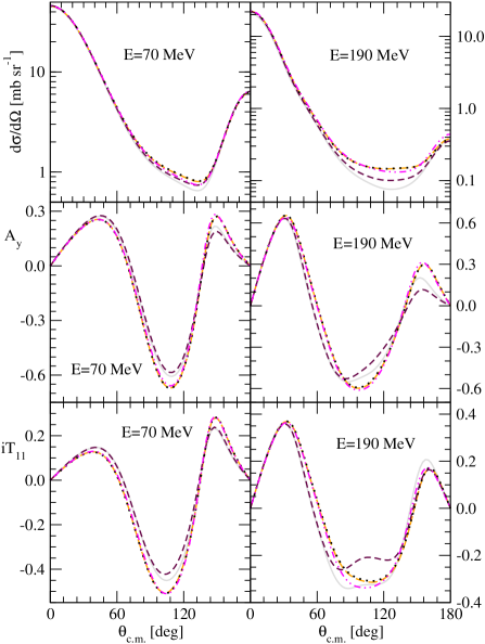
Figure 1: (color online) The angular distribution $\frac{d\sigma}{d\Omega}$, the neutron analyzing power $A_{y}$, and the deuteron vector analyzing power $iT_{11}$ in elastic nd scattering at the incoming neutron laboratory energy $E=70$ and $190$ MeV. The different curves are predictions of the chiral SMS N⁴LO⁺ NN potential with regulator $\Lambda=450$ MeV alone ((grey) solid line) or combined with the N²LO 3NF comprising also one contact term ${E_{7}}$ from N⁴LO. The exact prediction for that combination with strength parameters ($c_{D}=-8.2053,c_{E}=-1.0019,c_{E_{7}}=2.0$) is shown by the (orange) long dashed line. The exact predictions for parameter free term in N²LO 3NF (set of parameters ($c_{D}=0.0,c_{E}=0.0,c_{E_{7}}=0.0$) is shown by (maroon) short dashed line. The predictions based on approximate treatment with channels $|\beta\rangle$ restricted to only ${}^{1}S_{0}+^{3}S_{1}-^{3}D_{1}$ and to all $j_{max}=2$ channels, are represented by (magenta) dash-double-dotted and (black) dotted lines, respectively.

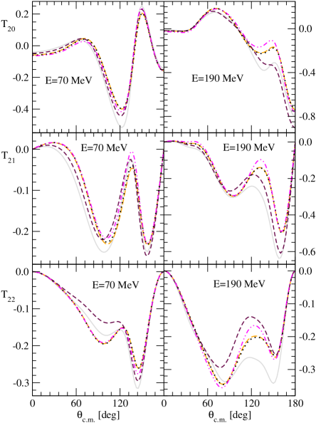
Figure 2: (color online) The same as in Fig. 1 but for deuteron tensor analyzing powers $T_{20},T_{21}$, and $T_{22}$.

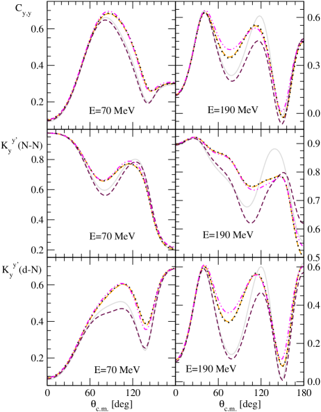
Figure 3: (color online) The same as in Fig. 1 but for the spin correlation $C_{y,y}$, polarization transfer coefficient from nucleon to nucleon $K_{y}^{y^{\prime}}(N-N)$, and polarization transfer coefficient from deuteron to nucleon $K_{y}^{y^{\prime}}(d-N)$.

.

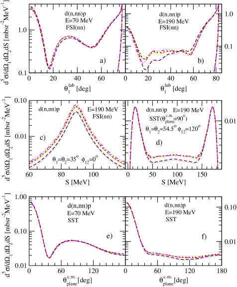
Figure 4: (color online) The exclusive breakup d(n,nn)p cross section $d^{5}\sigma/d\Omega_{1}d\Omega_{2}dS$ at the incoming neutron lab. energy $E=70$ and $190$ MeV for the neutron-neutron FSI condition ($\vec{p}_{1}=\vec{p}_{2}$) as a function of the lab. production angle of the outgoing neutrons $\theta_{1}^{lab}=\theta_{2}^{lab}$ and $\phi_{12}=0^{o}$: a), b), and for the SST condition as a function of the c.m. angle between plane, in which in the 3N c.m. frame momenta of three outgoing nucleons are placed, and the incoming nucleon momentum: e), f). In c) the cross sections for a particular FSI(nn) configuration from b) produced at $\theta_{1}^{lab}=\theta_{2}^{lab}=35^{o}$ and in d) for the SST from f) with $\theta_{plane}^{~{}c.m.}=90^{o}$ are shown along the arc-length S. For the description of lines see Fig. 1.