Determining the optimum thickness for high harmonic generation from nanoscale thin films: an ab initio computational study

Abstract

We theoretically investigate high harmonic generation (HHG) from silicon thin films with thicknesses from a few atomic layers to a few hundreds of nanometers, to determine the most efficient thickness for producing intense HHG in the reflected and transmitted pulses. For this purpose, we employ a few theoretical and computational methods. The most sophisticated method is the ab initio time-dependent density functional theory coupled with the Maxwell equations in a common spatial resolution. This enables us to explore such effects as the surface electronic structure and light propagation, as well as electronic motion in the energy band in a unified manner. We also utilize a multiscale method that is applicable to thicker films. Two-dimensional approximation is introduced to obtain an intuitive understanding of the thickness dependence of HHG. From these ab initio calculations, we find that the HHG signals are the strongest in films with thicknesses of 2–15 nm, which is determined by the bulk conductivity of silicon. We also find that the HHG signals in the reflected and transmitted pulses are identical in such thin films. In films whose thicknesses are comparable to the wavelength in the medium, the intensity of HHG signals in the reflected (transmitted) pulse is found to correlate with the magnitude of the electric field at the front (back) surface of the thin film.

I Introduction

Following progress in high harmonic generation (HHG) in atoms and molecules that enabled the production of attosecond pulses Corkum (1993); Lewenstein et al. (1994); Brabec and Krausz (2000); Krausz and Ivanov (2009), HHG in bulk crystals has attracted great interest during the last decade Ghimire and Reis (2019); Li et al. (2020). Experimental studies have achieved HHG in thin films of various materials and laser pulses Ghimire et al. (2011); Schubert et al. (2014); Vampa et al. (2015a); Hohenleutner et al. (2015); Luu et al. (2015); Langer et al. (2017); You et al. (2017); Shirai et al. (2018); Vampa et al. (2018a); Orenstein et al. (2019). These are extended to monatomic two-dimensional (2D) layers, such as graphene Yoshikawa et al. (2017, 2019), and to metasurfaces, periodic 2D structures composed of nanoscale objects Liu et al. (2018). HHG from bulk crystals is expected to be very intense compared with those from atoms in the gas phase because of the high atomic density. This indicates that the HHG from solids is favorable in applications to develop, for example, compact devices of XUV light sources.

Theoretical studies in the past mostly focused on electronic motion induced by a pulsed electric field prepared in advance Yu et al. (2019). For sufficiently thick films, it is legitimate to consider electronic motion in an infinitely periodic crystalline system in three dimensions induced by a spatially uniform electric field. Calculations employing theories of varying complexity, such as one-dimensional model, Hansen et al. (2017, 2018); Jin et al. (2019); Ikemachi et al. (2017), time-dependent Schrödinger equation Wu et al. (2015); Apostolova and Obreshkov (2018), density matrix models Ghimire et al. (2012); Vampa et al. (2014, 2015b), Floquet theory Faisal and Kamiński (1997); Faisal et al. (2005) and ab initio descriptions such as the time-dependent density functional theory (TDDFT) Otobe (2012, 2016); Tancogne-Dejean et al. (2017); Floss et al. (2018), have been developed. Theories to describe HHG from monatomic layers and bulk surfaces have also been developed Georges and Karatzas (2005); Le Breton et al. (2018). Using these theories, electronic motion in the wavenumber ($k$) space based on the energy band picture has been investigated and classified as inter- and intra-band motions Vampa et al. (2014). It has been clarified that there are rich manifestations of the crystalline structure of HHG through the band structure, selection rules, and dependence on the polarization direction Langer et al. (2017); You et al. (2017); Neufeld et al. (2019).

To investigate HHG in bulk materials, the propagation effect is also important. The light-propagation effect on HHG has been considered already in the case of atomic gases Popmintchev et al. (2009). However, the effect should be significant primarily in bulk solids, owing to their high atomic density. The propagation effect in HHG from thin films has been investigated recently. Experimentally, HHG in reflected and transmitted pulses has been measured and compared for films of several different thicknesses Vampa et al. (2018b); Xia et al. (2018). Theoretically, multiscale calculations coupling a coarse-graining electronic motion with light propagation have been conducted Ghimire et al. (2012); Zhokhov and Zheltikov (2017); Floss et al. (2018); Orlando et al. (2019); Kilen et al. (2020). It has been shown that the light propagation works to produce a clear HHG spectrum, even when the spectrum is unclear in the unit-cell calculation Floss et al. (2018). It has also been shown that the HHG in the transmitted pulse decreases by several orders of magnitude when emitted from thin films of micro-meter thickness Kilen et al. (2020).

Although there has been progress on the propagation effect, as described above, we consider that even the following basic questions have not yet been answered: (1) At what film thickness is HHG emitted with the maximum intensity? (2) What are the differences and similarities between HHGs in reflected and transmitted pulses? The principal purpose of this paper is to answer these questions unambiguously.

We theoretically describe HHG in Si thin films of various thicknesses, from a few atomic layers to a few hundreds of nanometers, that are comparable to the wavelength of the incident pulse in the medium. We utilize a few theoretical and computational frameworks based on ab initio TDDFT Runge and Gross (1984); Ullrich (2012) coupled with the Maxwell equations. In the most sophisticated method, we simultaneously solve the time-dependent Kohn-Sham (TDKS) equation for the electronic motion in TDDFT and the Maxwell equations for electromagnetic fields with a common spatial resolution. We call this the single-scale Maxwell-TDDFT method Yamada et al. (2018). The method is applicable to films with thicknesses of less than a few tens of nanometers because of its high computational cost. For thicker films, we utilize a multiscale Maxwell-TDDFT method, in which a microscopic TDKS equation is coupled with the macroscopic Maxwell equations with a coarse-graining approximation Yabana et al. (2012). A 2D approximation Yamada et al. (2018) is also introduced to obtain an intuitive understanding of the thickness dependence of HHG. Calculations using these methods provide a unified understanding on the HHG in nanoscale thin films.

This paper is organized as follows: Sec. II describes the theoretical and computational methods based on TDDFT. In Sec. III, the calculation results are presented. The thickness dependence of HHG, as well as the relation between HHGs in reflected and transmitted pulses, are discussed. Finally, a conclusion is presented in Sec. IV.

II Theoretical methods

II.1 Problem setup and method summary

We consider irradiation of a free-standing thin film of thickness $d$ in a vacuum by an ultrashort light pulse of a linearly polarized plane wave at normal incidence. As a prototypical material, we selected Si thin films of various thickness, from a few atomic layers to a few hundreds of nanometers. We assume that the thin film is infinitely periodic and macroscopically isotropic in 2D. The propagation and polarization directions of the incident light are taken to be along the $z$ and $x$ axes, respectively. We assume that the reflected and transmitted pulses contain only a component in the $x$ direction, owing to symmetry.

We express the asymptotic form of the vector potential in the following way using the $x$ component of the vector potential $A(z,t)$:

$$A(z,t)=\begin{cases}A^{\rm(i)}(t-z/c)+A^{\rm(r)}(t+z/c)&(z\rightarrow-\infty),\\ A^{\rm(t)}(t-z/c)&(z\rightarrow+\infty),\end{cases}$$ (1)

where $A^{\rm(i)}(t)$, $A^{\rm(r)}(t)$, and $A^{\rm(t)}(t)$ are the incident, reflected, and transmitted fields, respectively. The $x$ component of the electric field, $E(t)$, is related to the vector potential by $E(t)=-(1/c)dA(t)/dt$. The reflected and transmitted electric fields, $E^{\rm(r)}(t)$ and $E^{\rm(t)}(t)$, contain the high-order harmonics generated by the nonlinear light-matter interaction in the film.

To calculate HHG spectrum from a thin film theoretically, it has been commonly considered electronic motion in a unit cell of crystalline solids induced by an applied electric field whose time profile is prepared in advance. There are, however, a number of effects that should be considered further. We investigate the following three effects in this paper. First is an effect of the surface electronic structure, that is, a change of the electron band structure at the surfaces from that of the bulk system. The other two effects are related to the difference between the incident electric field $E^{\rm(i)}(t)$ and the electric field that actually acts on electrons in the thin film. We consider two effects that cause this difference. One is the effect of the light propagation. A strong incident laser pulse is modulated during the propagation due to nonlinear light-matter interactions, and HHG pulses that are generated inside the thin film also suffer from strong modulation and absorption during propagation before they exit the medium at the surfaces. The other is the effect of the conductivity of the thin film. Even when the thin film is so thin that the electric field inside the thin film can be regarded as uniform at the macroscopic scale, the electric field inside the film is different from that of the incident pulse due to the conductivity. Specifically, the current that flows in the film causes reflection from the film, and the electric field inside the medium is equal to the sum of the incident and reflected electric fields, not the incident field alone.

For a theoretical and computational description of HHG from a thin film, we utilize four ab initio approaches based on TDDFT Runge and Gross (1984); Ullrich (2012), which are summarized in Table I and explained in the following subsections. The simplest approach is the single unit-cell method, in which we solve the TDKS equation for electronic motion in a unit cell of the crystalline solid. In this description, the electric field of the incident pulse is used as an applied field. The most extensive and sophisticated approach is the single-scale Maxwell-TDDFT method Yamada et al. (2018), in which we solve the Maxwell equations for the electromagnetic fields and the TDKS equation for the electronic motion simultaneously using a common spatial grid. Here, all three effects mentioned above are included. In the multiscale Maxwell-TDDFT method Yabana et al. (2012), macroscopic light propagation and microscopic electronic motion are coupled using a coarse-graining approximation. In the practical calculation, the Maxwell equations and TDKS equation are solved simultaneously using different spatial grids. While the effect of the surface electronic structure is not included, this method can describe HHG from thick films that cannot be accessed by the single-scale Maxwell-TDDFT method. Finally, the 2D approximation Yamada et al. (2018) is introduced as an approximation to the multiscale Maxwell-TDDFT method, treating the thin film as an infinitely thin in macroscopic scale. This method will be useful to understand the thickness dependence of the HHG.

Table 1: Methods that will be used to describe HHG and their effectiveness to take account of various effects.

Theory	Single-scale Maxwell-TDDFT	Multiscale Maxwell-TDDFT	2D approximation	Single unit-cell
Treatment of EM fields	Microscopic	Macroscopic	2D macroscopic	None
Bulk electronic structure	Yes	Yes	Yes	Yes
Surface electronic structure	Yes	No	No	No
Light propagation	Yes	Yes	No	No
Conduction	Yes	Yes	Yes	No

II.2 Single unit-cell method

First, we consider a method describing the electronic motion in a unit cell of a crystalline solid under a spatially uniform electric field Bertsch et al. (2000); Otobe et al. (2008). This method describes electronic motion based on the energy-band picture, and has been utilized extensively to describe phenomena related to nonlinear and ultrafast dynamics of electrons such as nonlinear susceptibilities Uemoto et al. (2019), nonlinear energy transfer Yamada and Yabana (2019a), attosecond dynamics Wachter et al. (2014); Schultze et al. (2014); Yamada and Yabana (2020a), and HHG from various solids Otobe (2012, 2016); Tancogne-Dejean et al. (2017); Floss et al. (2018). Within the dipole approximation, the electron dynamics are described using the Bloch orbital of the bulk system, $u^{\rm bulk}_{n{\bm{k}}}({\bm{r}},t)$, where the wave vector ${\bm{k}}$ runs over the three-dimensional (3D) Brillouin zone of the unit cell. The TDKS equation for the Bloch orbitals $u^{\rm bulk}_{n{\bm{k}}}({\bm{r}},t)$ is written as

$$i\hbar\frac{\partial u^{\rm bulk}_{n{\bm{k}}}({\bm{r}},t)}{\partial t}=\biggl{\{}\frac{1}{2m}\left(-i\hbar\nabla+\hbar{\bm{k}}+\frac{e}{c}\hat{\bm{x}}A^{\rm(i)}(t)\right)^{2}$$

$$-e\phi({\bm{r}},t)+\delta\hat{V}_{\rm{ion}}+V_{\rm{xc}}({\bm{r}},t)\biggr{\}}u^{\rm bulk}_{n{\bm{k}}}({\bm{r}},t).\quad$$ (2)

Here, we use the vector potential of the incident pulse, $A^{\rm(i)}(t)$, as the applied electric field. The electric scalar potential $\phi({\bm{r}},t)$ includes the Hartree potential from the electrons and the local part of the ionic potential. $\delta\hat{V}_{\rm{ion}}$ and $V_{\rm{xc}}({\bm{r}},t)$ are the nonlocal part of the ionic pseudopotential Troullier and Martins (1991) and the exchange-correlation potential Perdew and Zunger (1981), respectively. All of the calculations within this paper are performed within the adiabatic local-density approximationOnida et al. (2002). We ignore the exchange-correlation effect for the vector potential, $A_{\rm xc}(t)$, for simplicity Ullrich (2012).

The electric current density averaged over the unit cell is calculated as follows:

$${\bm{J}}(t)=-\frac{e}{m}\int_{\Omega}\frac{d\bm{r}}{\Omega}\sum^{\rm occ}_{n{\bm{k}}}u^{\rm bulk\ast}_{n{\bm{k}}}({\bm{r}},t)$$

$$\times\left(-i\hbar\nabla+\hbar{\bm{k}}+\frac{e}{c}\hat{\bm{x}}A^{\rm(i)}(t)\right)u^{\rm bulk}_{n{\bm{k}}}({\bm{r}},t)+\delta{\bm{J}}(t),$$ (3)

where $\Omega$ is the volume of the unit cell and the index $n$ runs over the occupied band in the ground state. $\delta{\bm{J}}(t)$ is the current density from the nonlocal part of the pseudopotential Bertsch et al. (2000).

$$\delta{\bm{J}}(t) = -\frac{e}{m}\int\frac{d{\bm{r}}}{\Omega}\sum_{n{\bm{k}}}^{\rm occ}u^{\rm bulk\ast}_{n{\bm{k}}}({\bm{r}},t)e^{-i({\bm{k}}+(e/c)\hat{\bm{x}}A^{\rm(i)}(t)){\bm{r}}}$$ (4)

$$\times\frac{[{\bm{r}},\delta\hat{V}_{\rm ion}]}{i\hbar}e^{i({\bm{k}}+(e/c)\hat{\bm{x}}A^{\rm(i)}(t)){\bm{r}}}u^{\rm bulk}_{n{\bm{k}}}({\bm{r}},t).$$

In practice, the current contains only the $x$ component, parallel to the polarization direction of the incident pulse. We later discuss how to relate this current density with the HHG spectrum from a thin film of thickness $d$.

II.3 Single-scale Maxwell-TDDFT method

We next consider two theoretical methods that are capable of describing the electronic motion and light propagation simultaneously. The first is the single-scale Maxwell-TDDFT method, in which the electromagnetic fields are treated microscopically. In the next subsection, we will present the second method, the multiscale Maxwell-TDDFT method, in which the electromagnetic fields are treated macroscopically.

The single-scale Maxwell-TDDFT methodYamada et al. (2018) can fully account for the effects of the light propagation, conduction, and surface electronic structure. In this method, the Maxwell equations for electromagnetic fields and the TDKS equation for electronic motion are solved simultaneously in the time domain using a common spatial grid. In the present case, we consider an atomic configuration that is infinitely periodic in the $xy$ plane and isolated in the $z$ direction. The electronic motion is described using the Bloch orbital in the slab approximation, $u^{\rm slab}_{n{\bm{k}}}({\bm{r}},t)$, where ${\bm{k}}$ is the 2D crystal wave vector. This satisfies the following TDKS equation:

$$i\hbar\frac{\partial u^{\rm slab}_{n{\bm{k}}}({\bm{r}},t)}{\partial t}=\biggl{\{}\frac{1}{2m}\left(-i\hbar\nabla+\hbar{\bm{k}}+\frac{e}{c}{\bm{A}}({\bm{r}},t)\right)^{2}$$

$$-e\phi({\bm{r}},t)+\delta V_{\rm{ion}}({\bm{r}})+V_{\rm{xc}}({\bm{r}},t)\biggr{\}}u^{\rm slab}_{n{\bm{k}}}({\bm{r}},t).\quad$$ (5)

The vector potential ${\bm{A}}({\bm{r}},t)$ and the scalar potential $\phi({\bm{r}},t)$ are 2D periodic and satisfy the Maxwell equations in the Coulomb gauge:

$$\left(\frac{1}{c^{2}}\frac{\partial^{2}}{\partial t^{2}}-\nabla^{2}\right){\bm{A}}({\bm{r}},t)+\frac{1}{c}\frac{\partial}{\partial t}\nabla\phi({\bm{r}},t)=\frac{4\pi}{c}{\bm{j}}({\bm{r}},t),$$ (6)

$$\nabla^{2}\phi({\bm{r}},t)=-4\pi\rho({\bm{r}},t).$$ (7)

The vector potential ${\bm{A}}({\bm{r}},t)$ is smoothly connected to the asymptotic field of Eq. (1) at planes that are sufficiently separated from the medium. The scalar potential is chosen to be periodic in the $z$ direction as well as in the $x$ and $y$ directions. As mentioned above, all the dynamic variables, Bloch orbitals, and scalar and vector potentials are calculated using a common spacial grid without coarse graining. In this sense, both the vector and scalar potentials are treated microscopically in this approach.

The charge density $\rho({\bm{r}},t)$ and the electric current density ${\bm{j}}({\bm{r}},t)$ are derived from the Bloch orbitals, as follows:

$$\rho({\bm{r}},t) = \rho_{\rm ion}({\bm{r}})-e\sum_{n{\bm{k}}}^{\rm{occ}}|u^{\rm slab}_{n{\bm{k}}}({\bm{r}},t)|^{2},$$ (8)

$${\bm{j}}({\bm{r}},t) = -\frac{e}{m}{\rm Re}\sum_{n{\bm{k}}}^{\rm occ}u_{n{\bm{k}}}^{\rm slab\ast}({\bm{r}},t)\Bigl{(}-i\hbar\nabla$$ (9)

$$+\hbar{\bm{k}}+\frac{e}{c}{\bm{A}}({\bm{r}},t)\Bigr{)}u^{\rm slab}_{n{\bm{k}}}({\bm{r}},t),$$

where $\rho_{\rm ion}({\bm{r}})$ is the charge density of the ion cores. In this method, we ignore the current from the nonlocal part of the pseudopotentialYamada et al. (2018).

Because the Bloch orbitals $\{u^{\rm slab}_{n{\bm{k}}}({\bm{r}},t)\}$ are defined in the calculation box that includes entire film as well as the vacuum region, the size of the computation rapidly grows as the thickness of the film increases. In terms of the computational cost, applications of the single-scale Maxwell-TDDFT method is limited to thin films of thickness less than several tens of nanometers.

II.4 Multiscale Maxwell-TDDFT method

In the multiscale Maxwell-TDDFT method Yabana et al. (2012), macroscopic light propagation and microscopic electronic motion are coupled using a coarse-graining approximation. The light propagation is described using the following macroscopic wave equation:

$$\left(\frac{1}{c^{2}}\frac{\partial^{2}}{\partial t^{2}}-\frac{\partial^{2}}{\partial Z^{2}}\right)A_{Z}(t)=\frac{4\pi}{c}J_{Z}(t),$$ (10)

where $Z$ is the macroscopic coordinate. This wave equation is solved using a one-dimensional grid. At each grid point of $Z$, a bulk system with 3D periodicity is considered. The electronic motion at each grid point of $Z$ is described using 3D-periodic Bloch orbitals, $u^{\rm bulk}_{n{\bm{k}},Z}({\bm{r}},t)$, which satisfy the TDKS equation:

$$i\hbar\frac{\partial u^{\rm bulk}_{n{\bm{k}},Z}({\bm{r}},t)}{\partial t}=\biggl{\{}\frac{1}{2m}\left(-i\hbar\nabla+\hbar{\bm{k}}+\frac{e}{c}\hat{\bm{x}}A_{Z}(t)\right)^{2}$$

$$-e\phi_{Z}({\bm{r}},t)+\delta V_{\rm{ion}}({\bm{r}})+V_{\rm{xc},Z}({\bm{r}},t)\biggr{\}}u^{\rm bulk}_{n{\bm{k}},Z}({\bm{r}},t).\quad$$ (11)

From the Bloch orbitals, the averaged electric current density $J_{Z}(t)$ is calculated in the same manner as Eq. (3), but replacing $A^{\rm(i)}(t)$ with $A_{Z}(t)$.

At the beginning of the calculation, the Bloch orbitals at each grid point $Z$, $u^{\rm bulk}_{n{\bf k},Z}({\bm{r}},t)$, are set to the ground state. The vector potential $A_{Z}(t)$ is set to include only the incident pulse in the vacuum region. By solving Eqs. (10) and (11) simultaneously, we can evolve both $A_{Z}(t)$ and $u^{\rm bulk}_{n{\bm{k}},Z}({\bm{r}},t)$ simultaneously. We note that microscopic electronic systems at different $Z$ positions interact only through the vector potential $A_{Z}(t)$. When the light pulse is sufficiently weak and thus the perturbation approximation is applicable, the multiscale Maxwell-TDDFT method results in the ordinary macroscopic electromagnetism with the constitutive relation given by the dielectric function in the linear response TDDFT Yabana et al. (2012). The multiscale Maxwell-TDDFT method has been successfully applied to investigate a number of extremely nonlinear and ultrafast phenomena including attosecond science Lucchini et al. (2016); Sommer et al. (2016), saturable absorption Uemoto et al. (2021), coherent phonon generation and detection Yamada and Yabana (2019b, 2020b), and initial stage of nonthermal laser processing Sato et al. (2015).

In the multiscale Maxwell-TDDFT method, the effect of the light propagation can be taken into account while the effect of the surface electronic structure cannot. In compensation for the surface effect, the multiscale Maxwell-TDDFT method can be applied to thick films for which the single-scale Maxwell-TDDFT method is not capable. As we will show later, results of the multiscale Maxwell-TDDFT method coincide reasonably with those of the single-scale Maxwell-TDDFT method when the surface effect is not significant.

II.5 2D approximation

For sufficiently thin films, we may assume that the macroscopic electric field is spatially uniform inside the thin film. We call this the 2D approximation. This approximation is useful to identify and distinguish the conductive effect from the propagation effect, and to understand the thickness dependence of the HHG. The 2D approximation can be derived from the multiscale Maxwell-TDDFT method, as described below. Alternatively, it can also be derived from the single-scale Maxwell-TDDFT method, as explained in Ref Yamada et al., 2018.

We consider a film that is sufficiently thick to justify neglecting the effect of the surface electronic structure and sufficiently thin to regard the macroscopic electric field as spatially uniform in the film. In the next section, we see that there are thickness regions in which both assumptions are fulfilled simultaneously. Under these assumptions, the current density in Eq. (10) may be treated as

$$J_{Z}(t)\simeq\delta(Z)J(t)d,$$ (12)

where $d$ is the thickness of the film and $J(t)$ is the current density averaged over the unit cell. By inserting this current density into Eq. (10), we have

$$\left(\frac{1}{c^{2}}\frac{\partial^{2}}{\partial t^{2}}-\frac{\partial^{2}}{\partial Z^{2}}\right)A_{Z}(t)=\frac{4\pi}{c}\delta(Z)J(t)d.$$ (13)

This equationMishchenko (2009) should be solved with the asymptotic form of the vector potential of Eq. (1). In practice, the vector potential of Eq. (1) is the solution of Eq. (13), except at $Z=0$. The reflected and transmitted fields are determined by the connection conditions at $Z=0$. From the continuity of the vector potential at $Z=0$, we have

$$A^{\rm(i)}(t)+A^{\rm(r)}(t)=A^{\rm(t)}(t).$$ (14)

By integrating Eq. (13) once over $Z$, we obtain

$$\frac{dA^{\rm(t)}}{dt}=\frac{dA^{\rm(i)}}{dt}+2\pi dJ[A^{\rm(t)}](t)$$ (15)

at $Z=0$, where we denote the current density as $J[A^{\rm(t)}](t)$ to indicate that this is the current density caused by the vector potential $A_{Z=0}(t)=A^{\rm(t)}(t)$. This is the basic equation of the 2D approximation.

We note that this 2D approximation is equivalent to a specific case of the multiscale Maxwell-TDDFT method. If we take only a single grid point in the macroscopic coordinate $Z$ for the medium and choose the grid spacing to be equal to $d$, the calculation using the multiscale Maxwell-TDDFT method coincides with the above 2D approximation.

From the 2D approximation, we obtain several useful understandings regarding the HHG from very thin films. The continuity equation (14) indicates that the HHG spectra of the reflected and transmitted pulses are equal. Equation (15) indicates that the current density that creates HHG is produced by the transmitted pulse $A^{\rm(t)}(t)$, not the incident pulse of $A^{\rm(i)}(t)$, and the transmitted pulse itself is modulated by the current density. Even in very thin films such as monatomic layered films, the transmitted (and simultaneously, the reflected) fields are modulated by the current that flows in the film. This modulation significantly affects the HHG spectrum, as shown in the next section. We call this effect the conductive effect, as it is related to the electric current flowing in the thin film.

II.6 High harmonic generation spectrum

In the single-scale and multiscale Maxwell-TDDFT methods, we directly obtain the vector potentials of the reflected and the transmitted pulses. In the 2D approximation, we obtain the vector potentials of the transmitted pulse by Eq. (15). The vector potential of the reflected pulse is obtained by using the relation Eq. (14). From the vector potentials, we obtain the respective electric fields by taking the time derivative.

For the single unit-cell method, we will use the following expression for the reflected and transmitted electric fields.

$$E^{\rm(r)}(t)=E^{\rm(t)}(t)-E^{\rm(i)}(t)=-\frac{2\pi d}{c}J[A^{\rm(i)}](t).$$ (16)

This relation is derived if we replace $A^{\rm(t)}$ with $A^{\rm(i)}$ in $J[A^{\rm(t)}](t)$ of Eq. (15).

We evaluate the HHG spectra via the square of the Fourier-transformed electric field $|E^{\rm(r,t)}(\omega)|^{2}$, where $E^{\rm(r,t)}(\omega)$ is defined by,

$$E^{\rm(r,t)}(\omega)=\int_{t_{0}}^{t_{0}+T}dt\,e^{i\omega t}E^{\rm(r,t)}(t)\,f\left(\frac{t-t_{0}}{T}\right).$$ (17)

Here, $f(x)\equiv 1-3x^{2}+2x^{3}$ is a smoothing functionYabana et al. (2006) and $t_{0}$ is the initial time. For the reflection pulse, $t_{0}$ is set to the initial time of the incident pulse. For the transmitted pulse, the time delay by transmission is added to $t_{0}$ for thick films. When we discuss the thickness dependence of HHG, we introduce the strength of the $n$th-order harmonics, as follows:

$$I_{n}^{\rm(r,t)}=\int^{\left(n+\frac{1}{2}\right)\omega_{0}}_{\left(n-\frac{1}{2}\right)\omega_{0}}d\omega\,|E^{\rm(r,t)}(\omega)|^{2},$$ (18)

where $\omega_{0}$ is the fundamental frequency.

II.7 Numerical detail

For numerical calculations, we utilize the open-source software SALMON (Scalable Ab initio Light-Matter simulator for Optics and Nanoscience)Noda et al. (2019); SAL developed by our group. In this code, electronic orbitals as well as electromagnetic fields are expressed using a uniform 3D spatial grid. The time evolution of the electron orbitals is carried out using the Taylor expansion method Yabana and Bertsch (1996).

In the single unit-cell method, we use a cubic unit cell that contains eight Si atoms with the side length of $a=0.543$ nm. To express the Bloch orbitals, a spatial grid of $16^{3}$ points is used. The 3D Brillouin zone is sampled by a $24^{3}$ $k$-point grid. The time step is set to $2.5\times 10^{-3}$ fs.

The same cubic unit cell is also used in the 2D approximation and multiscale Maxwell-TDDFT method. In the multiscale Maxwell-TDDFT method, a uniform 1D grid is also introduced to describe the wave equation of Eq. (10), with the grid spacing less than or equal to $6.25$ nm.

In the single-scale Maxwell-TDDFT method, the 2D-periodic box of the size of $a\times a\times(d+4a)$ is used where the size along the $z$ axis contains the vacuum region of $4a$ in the slab approximation. The atomic positions of Si atoms are set at those positions in the bulk crystalline system, and the dangling bonds at the surfaces are terminated by hydrogen atoms. A uniform 3D spatial grid is used with the same grid spacing as that in the cubic unit cell. The 2D Brillouin zone of the single-scale Maxwell-TDDFT method is sampled by a $24\times 24$ $k$-point grid.

III Results and discussion

III.1 HHG in reflected and transmitted pulses

We employ the following time profile for the incident pulse:

$$A^{\rm(i)}(t)=-\frac{cE_{0}}{\omega_{0}}\,\sin\omega_{0}t\,\,\cos^{6}\left(\frac{\pi t}{T}\right),\,(-\frac{T}{2}<t<\frac{T}{2}),$$

(19)

where $E_{0}$ is the maximum amplitude of the electric field, $\omega_{0}$ is the average frequency, and $T$ is the pulse duration. In the following calculations, we set $\hbar\omega_{0}=$ 1.5 eV and $T=$ 30 fs.

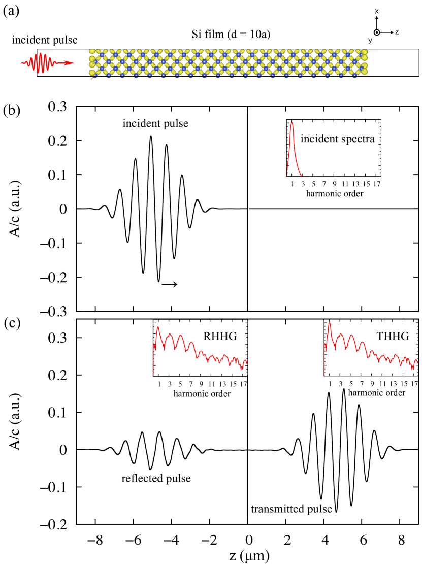
Figure 1: Typical calculation using the single-scale Maxwell-TDDFT method for a Si thin film of thickness $d=10a$ (5.43 nm). (a) Electron density in the ground state in a plane containing Si atoms. (b) Initial pulse set to the left of the thin film located at $z=0$. The peak intensity of the pulse is set at $I=5\times 10^{12}$ W/cm² at $t=0$. (c) Reflected and transmitted pulses at $t=31.25$ fs. The insets show the corresponding HHG spectra.

For a typical case, Figure 1 shows snapshots of the incident pulse [Eq. (19)] and the transmitted and the reflected pulses in the calculation using the single-scale Maxwell-TDDFT method for a film of thickness $d=10a$ (5.43 nm). The maximum amplitude $E_{0}$ of the incident pulse is set to provide the peak intensity of $I=5\times 10^{12}$ W/cm². In Fig. 1(a), the electronic density at the ground state in a plane that includes Si atoms is shown. In Fig. 1(b), the incident pulse is prepared to the left of the thin film located at $z=0$. Figure 1(c) shows the pulses at a sufficient time after interaction. The reflected (transmitted) pulse is seen in the left (right) to the film. The insets show spectra for the respective pulses. It can be clearly seen that the reflected and the transmitted pulses include HHG signals.

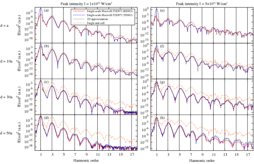
Figure 2: HHG spectra in the reflected pulse (RHHG) and the transmitted pulse (THHG). Left panels [(a)–(d)] show the spectra for a pulse with the peak intensity of $I=1\times 10^{12}$ W/cm² and right panels [(e)–(h)] for a pulse of $I=5\times 10^{12}$ W/cm². Top panels [(a), (e)] show the spectra for the film thickness of $d=a$ (0.543 nm), second panels [(b), (f)] for $d=10a$ (5.43 nm), third panels [(c), (g)] for $d=30a$ (16.29 nm), and bottom panels [(d), (h)] for $d=50a$ (27.15 nm). The red solid (blue dashed) line for the RHHG (THHG) using the single-scale Maxwell-TDDFT method, blue dotted line using the 2D approximation, and orange dash-dotted line using the single unit-cell method.

We first discuss thin films with thicknesses less than a few tens of nanometers. For such films, it is possible to achieve calculations using the single-scale Maxwell-TDDFT method. Figure 2 shows the HHG spectra included in the reflected (RHHG) and transmitted (THHG) pulses. The left panels [Fig. 2(a)–(d)] show the spectra for the incident pulse with a peak intensity of $I=1\times 10^{12}$ W/cm², and the right panels [Fig. 2(e)–(h)] show those for a peak intensity of $5\times 10^{12}$ W/cm². Panels (a) and (e) show results for the film of thickness $d=a$ (0.543 nm), (b) and (f) for $10a$ (5.43 nm), (c) and (g) for $30a$ (16.29 nm), and (d) and (h) for $50a$ (27.15 nm). The red solid line (blue dashed line) shows RHHG (THHG) using the single-scale Maxwell-TDDFT method, and the black dotted line shows HHG using the 2D approximation [Eq. (15)]. In the 2D approximation, the HHG spectra in the reflected and transmitted pulses coincide, except for the component of the fundamental frequency $\omega_{0}$. The orange dash-dotted line shows the HHG spectrum using the single unit-cell method.

First, we focus on the extremely thin case of $d=a$ (0.543 nm) [Fig. 2(a), (e)]. This is a film composed of two atomic layers. Although fabrication of such thin material composed of Si is not easy, HHG of such thin materials is highly concerned, as measurements and calculations have been reported for a number of 2D materials such as graphene and transition metal dichalcogenides Yoshikawa et al. (2017, 2019); Sato et al. (2021). Here the RHHG and the THHG spectra using the single-scale Maxwell-TDDFT method coincide accurately, as expected from the argument in the 2D approximation [Eq. (14)]. However, the HHG spectrum by the 2D approximation (black dotted line) does not coincide accurately with that using the single-scale Maxwell-TDDFT method. This indicates the significance of the effect of the surface electronic structure that is not included in the 2D approximation. We note that the validity of the relation of Eq. (14) does not suffer by the surface electronic structure, as it can be derived directly from the single-scale Maxwell-TDDFT methodYamada et al. (2018). The result of the single unit-cell method (orange dash-dotted line) coincides with the 2D approximation, indicating that the conductive effect in the film is not important in such extremely thin film.

The above observations hold also at the film of thickness $d=10a$ (5.43 nm) [Fig. 2(b), (f)], except that the discrepancy between spectra using the 2D approximation and the single unit-cell method becomes apparent. It implies that the effect of the conductivity in the thin film, use of $A^{\rm(t)}$, not the incident pulse $A^{\rm(i)}$, to evaluate the current in the right hand side of Eq. (15), increases as the film thickness increases, because the effect is proportional to $d$.

In the case of $d=30a$ (16.29 nm) [Fig. 2(c), (g)], the results using the single-scale Maxwell-TDDFT method and those using the 2D approximation agree reasonably with each other. This indicates that neither the surface electronic structure nor the propagation effect is significant at this thickness. Only the conductive effect is important. By closely observing the difference between the RHHG and THHG spectra, the latter is slightly greater than the former. This indicates that the propagation effect starts to appear.

In the case of $d=50a$ (27.15 nm) [Fig. 2(d), (h)], it is clear that, in the single-scale Maxwell-TDDFT method, the THHG is greater than the RHHG due to the propagation effect. Now the calculation using the single unit-cell method greatly differs from the others, despite the 2D approximation still reasonably reproduces the results using the single-scale Maxwell-TDDFT method. Looking into detail, the spectrum of the 2D approximation is closer to the THHG in the single-scale Maxwell-TDDFT method than the RHHG. The high-order part of the spectrum shown in Fig. 2(d) [and partially Fig. 2(c)] looks noisy, presumably because the driving field is too weak ($I=1\times 10^{12}$ W/cm²) to produce high-order signals at this thickness.

Overall, the 2D approximation is a reasonable approximation to the single-scale Maxwell-TDDFT method in this thickness region. This indicates that the surface electronic structure and the propagation effects are not significant. The large difference between the results using the 2D approximation and those using the single unit-cell method indicates that the conductive effect is significant, even in these very thin films.

By comparing the different thicknesses, especially Fig. 2(e) and (f)–(h), we realize that the HHG spectrum is unclear in films of thickness $d=a$ (0.543 nm) and becomes clearer as the thickness increases. This trend is common in both spectra using the single-scale Maxwell-TDDFT method and the 2D approximation. It implies that the conductive effect, the current in the thin film that appears in the right hand side of Eq. (15), contributes to produce a cleaner HHG signal. This is consistent with the observation in Ref Floss et al., 2018 where both the conductive and the propagation effects are included.

III.2 Thickness dependence

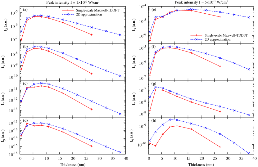
Figure 3: Thickness dependence of HHG intensities is shown from 3rd [(a), (e)], 5th [(b), (f)], 7th [(c), (g)], and 9th [(d), (h)] orders included in the reflected pulse. Left panels [(a)–(d)] for the incident pulse of the peak intensity at $I=1\times 10^{12}$W/cm², and right panels [(e)–(h)] at $I=5\times 10^{12}$W/cm². Results using single-scale Maxwell-TDDFT method are shown by red solid lines, and results using 2D approximation are shown by blue-dashed lines.

Figure 3 shows the thickness dependence of the intensity of HHG in the reflected pulse using Eq. (18). The peak intensity of the incident pulses is set at $I=1\times 10^{12}$ W/cm² in Fig. 3(a)–(d) and at $5\times 10^{12}$ W/cm² in Fig. 3(e)–(h). Intensities of harmonic order of 3rd [(a), (e)], 5th [(b), (f)], 7th [(c), (g)], and 9th [(d), (h)] are shown. The red solid line (blue dashed line) corresponds to the single-scale Maxwell-TDDFT method (2D approximation).

As seen from Fig. 3, the thickness dependence of HHG intensities using the 2D approximation (blue dashed line) shows qualitative agreement with those using the single-scale Maxwell-TDDFT method (red solid line). In both calculations, the HHG intensity is maximum around thicknesses of $d=$ 2–15 nm, irrespective of the order of the HHG. The appearance of the maximum at these thicknesses can be understood as a consequence of the conductive effect, as described below, extending the formalism of the 2D approximation.

By taking the Fourier transform of Eq. (15), we obtain

$$-i\omega A^{\rm(t)}(\omega)=-i\omega A^{\rm(i)}(\omega)+2\pi d\,\,J[A^{\rm(t)}](\omega).$$ (20)

We decompose the current density into linear and nonlinear components as $J[A^{\rm(t)}](\omega)=J_{\rm L}[A^{\rm(t)}](\omega)+J_{\rm NL}[A^{\rm(t)}](\omega)$ and use the constitutive relation for the linear part,

$$J_{\rm L}[A^{\rm(t)}](\omega)=\sigma(\omega)E^{\rm(t)}(\omega)=\frac{i\omega}{c}\sigma(\omega)A^{\rm(t)}(\omega),$$ (21)

where $\sigma(\omega)$ is the conductivity of the bulk medium. Combining the above equations, we obtain

$$\left(1+\frac{2\pi d}{c}\sigma(\omega)\right)A^{\rm(t)}(\omega)=A^{\rm(i)}(\omega)+\frac{2\pi id}{\omega}J_{\rm NL}[A^{\rm(t)}](\omega).$$ (22)

We also decompose the transmitted vector potential into linear and nonlinear components Yamada et al. (2018), $A^{\rm(t)}(\omega)=A_{\rm L}^{\rm(t)}(\omega)+A_{\rm NL}^{\rm(t)}(\omega)$, where the linear vector potential is given by

$$A^{\rm(t)}_{\rm L}(\omega)=\left(1+\frac{2\pi d}{c}\sigma(\omega)\right)^{-1}A^{\rm(i)}(\omega).$$ (23)

The nonlinear term $A^{\rm(t)}_{\rm NL}$ satisfies the following relation:

$$A^{\rm(t)}_{\rm NL}(\omega)=\frac{2\pi id}{\omega}\left(1+\frac{2\pi d}{c}\sigma(\omega)\right)^{-1}J_{\rm NL}[A^{\rm(t)}_{\rm L}+A^{\rm(t)}_{\rm NL}](\omega).$$ (24)

We note that the nonlinear component of the reflected pulse is also given by Eq. (24). So far, no approximations have been made besides the 2D approximation. Here, we assume that the nonlinear component $A^{\rm(t)}_{\rm NL}$ is rather small and can be ignored to evaluate the nonlinear current density in the right hand side of Eq. (24). Then, we have

$$A^{\rm(t)}_{\rm NL}(\omega)\simeq\frac{2\pi id}{\omega}\left(1+\frac{2\pi d}{c}\sigma(\omega)\right)^{-1}J_{\rm NL}[A^{\rm(t)}_{\rm L}](\omega).$$ (25)

To investigate how the HHG intensity included in the above $A^{\rm(t)}_{\rm NL}(\omega)$ depends on $d$, we introduce two further assumptions. First, we assume that the incident pulse $A^{\rm(i)}(t)$ has a well-defined frequency, which we denote as $\omega_{0}$. Second, the $n$th-order nonlinear current density is proportional to $A^{n}$, where $A$ is the amplitude of the vector potential. Then, from Eq. (23), the $d$ dependence of the $n$th-order term in $J_{\rm NL}[A^{\rm(t)}_{\rm L}](\omega)$ is given by $(1+2\pi\sigma(\omega_{0})\,d/c)^{-n}$. Then, from Eq. (25), the $n$th-order term of $A^{\rm(t)}_{\rm NL}(\omega=n\omega_{0})$ is proportional to the following factor:

$$A^{\rm(t)}_{\rm NL}(n\omega_{0})\propto\frac{d}{\left(1+\frac{2\pi\sigma(n\omega_{0})}{c}d\right)\left(1+\frac{2\pi\sigma(\omega_{0})}{c}d\right)^{n}}.$$ (26)

From this $d$ dependence, we expect that the intensity of the HHG of each order shows a maximum as a function of $d$, and the peak position is determined by the bulk conductivity.

The conductivity at the frequency of the HHG, $\sigma(n\omega_{0})$, depends on the order $n$ and becomes small at high orders, $n>>1$. For simplicity, we consider the $d$-dependence caused by the conductivity at the fundamental frequency, $\sigma(\omega_{0})$. We expect the peak of HHG appears at the thickness,

$$d\sim\frac{c}{2\pi\sqrt{n-1}|\sigma(\omega_{0})|},$$ (27)

where we used $\sigma(\omega_{0})$ as a pure imaginary number at the frequency $\hbar\omega_{0}=1.5$ eV. The value $c/(2\pi|\sigma(\omega_{0})|)\simeq 19.2$ nm is derived from the conductivity of Si at the frequency $\omega_{0}$. This explains the appearance of the peak around $d=$ 2–15 nm.

III.3 Propagation effect

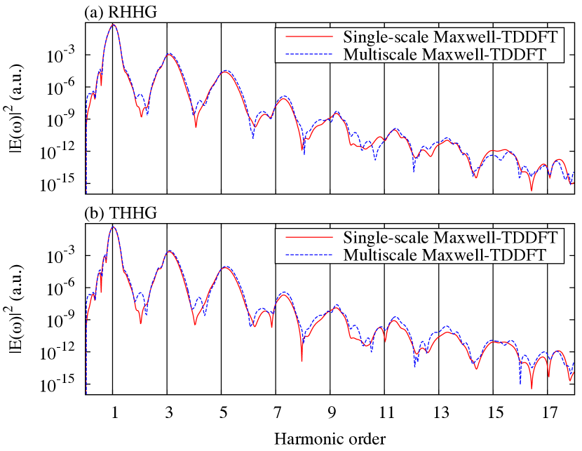
Figure 4: HHG spectra of $d=50a$ (27.19 nm) film included in the reflected (a) and the transmitted (b) pulses are shown. Red solid lines show the results using the single-scale Maxwell-TDDFT method, whereas the blue dashed lines show those using the multiscale Maxwell-TDDFT method.

As the film thickness increases, the computational cost of the single-scale Maxwell-TDDFT method rapidly increases. Therefore, the use of the multiscale Maxwell-TDDFT method is appropriate and necessary. To confirm the accuracy of the multiscale method, we compare the two methods in Fig. 4 for RHHG and THHG emitted from a film of thickness $d=50a$ (27.19 nm) and the incident pulse with maximum intensity $I=5\times 10^{12}$ W/cm², which is the same conditions as those in Fig. 2(h). Because the spectra using two methods coincide accurately with each other, we may conclude that the multiscale Maxwell-TDDFT method, which ignores the effect of the surface electronic structure, is reliable for films of this thickness and greater.

We note that, as mentioned in Sec. II.C, the multiscale Maxwell-TDDFT method is identical to the 2D approximation for very thin films where the macroscopic electric field may be regarded as uniform inside the thin film. As discussed in Fig. 2, the 2D approximation was a good approximation for films of thickness less than $d=50a$ (27.19 nm). In summary, we expect the multiscale Maxwell-TDDFT method to be reliable for thin films of any thickness as long as the surface electronic structure is not important.

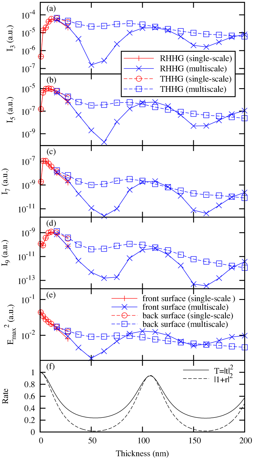
Figure 5: (a)–(d) Thickness dependence of the intensities of the reflected (solid lines with crosses) and the transmitted (dashed lines with squares) HHG, from 3rd (a) to 9th (d) order. Red lines and symbols are calculated using the single-scale Maxwell-TDDFT method, and blue lines and symbols using the multiscale Maxwell-TDDFT method. (e) Maximum intensities of the electric fields averaged over the 2D area of the front (back) surface are shown by red lines with symbols (blue lines with symbols). (f) Intensities of electric fields in ordinary electromagnetism at the front (back) surface are shown by dashed (solid) lines.

Figure 5(a)–(d) shows the thickness dependence of the third- to ninth-order harmonics included in the reflected and transmitted pulses for the incident pulse with a peak intensity of $I=5\times 10^{12}$ W/cm². Results using the single-scale Maxwell-TDDFT method are shown for thickness $d\leq 50a$ (27.19 nm). The RHHG shown here are the same as those in Fig. 3(e)–(h). The results using the multiscale Maxwell-TDDFT method are shown for thickness $d\geq 30a$ (16.29 nm).

Figure 5(e) shows the square of the maximum electric field amplitude in time, $E_{\rm max}=\max_{t}|E(t)|$, at the front surface and the back surface of the film. When using the single-scale Maxwell-TDDFT method, an average over the surface is taken. Figure 5(f) shows $|t|^{2}$ and $|1+r|^{2}$, where $t$ and $r$ are the amplitude of transmission and reflection coefficients in ordinary electromagnetism:

$$r=\frac{r_{0}(1-e^{2i\phi})}{1-r_{0}^{2}e^{2i\phi}},\hskip 14.22636ptt=\frac{(1-r_{0}^{2})e^{i\phi}}{1-r_{0}^{2}e^{2i\phi}},$$ (28)

where $r_{0}=(1-n)/(1+n)$ and $\phi=2\pi nd/\lambda$. The index of refraction $n$ of Si and the wavelength $\lambda$ is evaluated at the frequency $\omega_{0}$. $T=|t|^{2}$ is equal to the transmittance and is equal to the square of the electric field at the back surface, while $|1+r|^{2}$ is equal to the square of the electric field at the front surface.

Because the frequency $\omega_{0}$ is below the direct bandgap of Si, $|t|^{2}$ and $|1+r|^{2}$ become unity when $2\pi nd$ is equal to the wavelength and its integer multiples. As seen from Fig. 5(e), however, the magnitude of the electric field at the back surface decreases monotonically as the film thickness increases in the Maxwell-TDDFT calculations. The magnitude of the electric field at the front surface shows more oscillatory behavior, with a clear minimum at $\pi d=\lambda$. However, the magnitude is smaller at $\pi d=2\lambda$ than at the zero-thickness limit. These decreases originate the nonlinear propagation effect included in both the single-scale and multiscale Maxwell-TDDFT methods. In any case, the magnitude of the electric field at neither the front nor the back surface exceeds the magnitude of the electric field at the zero-thickness limit.

The intensities of RHHG and THHG coincide with each other when the film is sufficiently thin. As discussed previously, they are well understood by Eq. (14) and start to deviate at a distance of 10–20 nm. As seen from Fig. 5, except the $d<20$ nm region, the thickness dependence of RHHG (THHG) is correlated faithfully with the maximum electric field at the front (back) surface. This indicates that the magnitude of the RHHG and the THHG is determined simply by the intensity of its driving electric field at the respective surfaces. Because the magnitude of the electric field at the front or back surface does not exceed those at the zero-thickness limit, the maximum of the intensity of the HHG signals also appears around $d\sim 10$ nm as seen in Fig. 3.

IV Conclusion

We have developed a few theoretical and computational methods based on first-principles TDDFT and investigated HHG from thin films of crystalline solids with thicknesses from a few atomic layers to a few hundreds of nanometers. Using these methods, it is possible to investigate effects of (1) surface electronic structure, (2) conductivity of the film, and (3) light propagation of fundamental and high-harmonic fields, as well as (4) the effect of electronic motion in the bulk energy band.

Among methods used herein, the most sophisticated method is the single-scale Maxwell-TDDFT method, which considers all four effects mentioned above. It can be applied to thin films with thicknesses less than a few tens of nanometers. For thicker films, the multiscale Maxwell-TDDFT method, in which a coarse-graining approximation is introduced, is applicable. It can treat the effects except for the surface electronic structure. To achieve insight into the thickness dependence of the HHG, the 2D approximation is useful. We applied these methods to thin films of crystalline silicon as a prototype material, and obtained the following conclusions.

For thin films with thicknesses less than a few tens of nanometers, HHG spectra of reflected and transmitted pulses are almost identical. This could be understood from the 2D approximation. In extremely thin films, the HHG intensity increases as the thickness of the film increases. However, the intensity soon saturates and reaches its maximum at a thickness of around 2–15 nm. The saturation of the intensity originates from the current that flows in the thin film and can be described using the bulk linear conductivity of the medium. This conductive effect also creates a clean HHG spectrum.

As the thickness increases beyond a few tens of nanometers, it is found that the intensity of the reflected (transmitted) HHG strongly correlates with the intensity of the electric field at the front (back) surface of the thin film. By reflecting the interference effect in pulse propagation, we find an enhancement in the reflected HHG when the film thickness is equal to integer or half-integer multiples of the fundamental wavelength in the medium, $\lambda/n$, where $n$ is the index of refraction. However, the transmitted HHG monotonically decreases as the thickness increases, owing to the nonlinear propagation of the fundamental wave.