Arbitrarily High-order Maximum Bound Preserving Schemes with Cut-off Postprocessing for Allen-Cahn Equations

Abstract

We develop and analyze a class of maximum bound preserving schemes for approximately solving Allen–Cahn equations. We apply a $k$th-order single-step scheme in time (where the nonlinear term is linearized by multi-step extrapolation), and a lumped mass finite element method in space with piecewise $r$th-order polynomials and Gauss–Lobatto quadrature. At each time level, a cut-off post-processing is proposed to eliminate extra values violating the maximum bound principle at the finite element nodal points. As a result, the numerical solution satisfies the maximum bound principle (at all nodal points), and the optimal error bound $O(\tau^{k}+h^{r+1})$ is theoretically proved for a certain class of schemes. These time stepping schemes under consideration includes algebraically stable collocation-type methods, which could be arbitrarily high-order in both space and time. Moreover, combining the cut-off strategy with the scalar auxiliary value (SAV) technique, we develop a class of energy-stable and maximum bound preserving schemes, which is arbitrarily high-order in time. Numerical results are provided to illustrate the accuracy of the proposed method.

Keywords: Allen-Cahn equation, single step methods, lumped mass FEM, cut off, high-order, maximum bound preserving, energy-stable.

AMS subject classifications 2010: 65M30, 65M15, 65M12

1 Introduction

The aim of this paper is to design and analyze a high-order maximum bound preserving (MBP) scheme for solving the Allen–Cahn equation:

(1) $$\begin{cases}u_{t}=\Delta u+f(u)&\mbox{in~{}~{}}\Omega\times(0,T),\\ u(x,t=0)=u_{0}(x)&\mbox{in~{}~{}}\Omega\times\{0\},\\ \partial_{\mathbf{n}}u=0&\mbox{on~{}~{}}\partial\Omega\times(0,T)\\ \end{cases}$$

where $\Omega$ is a smooth domain in $\mathbb{R}^{d}$ with the boundary $\partial\Omega$. $f(u)=-F^{\prime}(u)$ with a double-well potential $F$ that has two wells at $\pm\alpha$, for some known parameter $\alpha>0$. For two popular choices of potentials. It is well-known that the Allen–Cahn equation (1) has the maximum bound principle [7]:

(2) $$|u_{0}(x)|\leq\alpha\quad\Longrightarrow\quad|u(x,t)|\leq\alpha\qquad\text{for all}~{}~{}(x,t)\in\Omega\times(0,T].$$

As a typical $L^{2}$ gradient flow associating with the following free energy

$$E(u)=\int_{\Omega}\frac{1}{2}|\nabla u|+F(u)\mathrm{d}x,$$

the nonlinear energy dissipation law holds in the sense

(3) $$\frac{\mathrm{d}}{\mathrm{d}t}E(u)=-\int_{\Omega}|u_{t}|^{2}\mathrm{d}x\leq 0.$$

The Allen–Cahn equation was originally introduced by Allen and Cahn in [2] to describe the motion of anti-phase boundaries in crystalline solids. In the context, $u$ represents the concentration of one of the two metallic components of the alloy and the parameter $\varepsilon$ involved in the nonlinear term represents the interfacial width, which is small compared to the characteristic length of the laboratory scale. Recent decades, the Allen–Cahn equation has become one of basic phase-field equations, which has been widely applied to many complicated moving interface problems in materials science and fluid dynamics through a phase-field approach coupled with other models [3, 5, 31].

1.1 Review on existing studies

The development and analysis of MBP method have been intensively studied in existing references. It was proved in [27, 23] that the stabilized semi-implicit Euler time-stepping scheme, with central difference method in space, preserves the maximum principle unconditionally if the stabilizer satisfies certain restrictions. In [6], a stabilized exponential time differencing scheme was proposed for solving the (nonlocal) Allen–Cahn equation, and the scheme was proved to be unconditionally MBP. See also [7] for the generalization to a class of semilinear parabolic equations. The second-order backward differentiation formula (with nonuniform meshes) was applied to develop an MBP scheme in [17] under the usual CFL condition $\tau=O(h^{2})$.

High-order strong stability preserving (SSP) time-stepping methods are widely used in the development of MBP scheme for both parabolic equations and hyperbolic equations (see e.g., [11, 18, 12, 10, 19, 21, 30, 32]). Recently, an SSP integrating factor Runge–Kutta method of up to order four was proposed and analyzed in [14] for semilinear hyperbolic and parabolic equations. For semilinear hyperbolic and parabolic equations with strong stability (possibly in the maximum norm), the method can preserve this property and can avoid the standard parabolic CFL condition $\tau=O(h^{2})$, only requiring the stepsize $\tau$ to be smaller than some constant depending on the nonlinear source term, also referring to [15]. A nonlinear constraint limiter was introduced in [29] for implicit time-stepping schemes without requiring CFL conditions, which can preserve maximum principle at the discrete level with arbitrarily high-order methods by solving a nonlinearly implicit system.

Very recently, a new class of high-order MBP methods was proposed in [16]. The method consists of a $k$th-order multistep exponential integrator in time, and a lumped mass finite element method in space with piecewise $r$th-order polynomials. At every time level, the extra values exceeding the maximum bound are eliminated at the finite element nodal points by a cut-off operation. Then the numerical solution at all nodal points satisfies the MBP, and an error bound of $O(\tau^{k}+h^{r})$ was proved. However, numerical results in [16, Table 4.1] indicates that the error bound is not sharp in space, and how to improve the estimate it is still open. Besides, the aforementioned scheme requires to evaluate some actions of exponential functions of diffusion operators, which might be relatively expensive compared with solving poisson problems, and the generalization to other time stepping schemes is a nontrivial task. Finally, the proposed scheme (with relatively coarse step sizes) might produce a numerical solution with obviously increasing and oscillating energy. These motivate our current project.

1.2 Our contributions and the organization of the paper

The first contribution of the current paper is to develop and analyze a class of MBP schemes, which could be arbitrarily high-order in both space and time, for approximately solving the Allen–Cahn equation (1). In time, we apply a single-step method, which is (strictly) accurate of order $k$, and apply multistep extrapolation to linearize the nonlinear term. In space, we apply the lumped mass FEM with piecewise $r$th-order polynomials and Gauss–Lobatto quadrature, as in [16]. At each time level, we apply a cut-off operation to remove the extra value exceeding the maximum bound at the nodal points. We estabilish the error estimate of order $O(\tau^{k}+h^{r+1})$, which fills the gap between the numerical results in [16, Theorem 3.2] showing optimal convergence rate $O(h^{r+1})$ and the theoretical result in [16, Table 4.1] providing only a suboptimal error estimate of order $O(h^{r})$. The improvement follows from a careful examination of quadrature errors (see Remark 2.4 and [16, eq. (2.6) and (3.22)]). To the best of our knowledge, this is the first work deriving optimal error estimates of arbitrarily high-order MBP schemes for the Allen–Cahn equation (1).

Nevertheless, the optimal estimate of the fully discrete scheme (with the cut-off postprocessing) requires the L-stability of the time stepping scheme, which excludes some popular and practical singe step method, e.g. Gauss–Legendre method belonging to algebraically stable collocation Runge–Kutta method. Therefore, we revisit this class of time stepping methods and prove the same error estimate by using the energy argument without using the L-stability. This is the second contribution of the paper.

In case of relative coarse step sizes, the proposed time stepping scheme (with the cut-off operation at each time level) might result in oscillating and increasing energy (see e.g. Figure 2 (middle)), which violates the energy dissipation law (3) of Allen–Cahn equation (1). This motivates us to develop a class of energy-stable and MBP schemes, by combining the cut-off strategy with the scalar auxiliary value (SAV) method [26]. The scheme is second order in space but could be arbitrarily high-order in time. As far as we know, this is the first scheme that is unconditionally energy-dissipative, maximum bound preserving, and arbitrarily high-order in time scheme with a provable error bound. In fact, our numerical results show that the use of SAV regularizes the numerical solution, stabilizes the energy, and significantly reduces the cut-off values at each time level (see e.g. Figure 2).

The rest of the paper is organized as follows. In section 2, we consider the single step methods (in a general framework) with cut-off postprocessing and multistep extrapolation. Error estimate for both semidiscrete and fully discrete scheme are provided, where the optimal error estimate of the fully discrete scheme requires the L-stability of the time stepping scheme. In section 3, we analyze the algebraically stable collocation scheme and show the same error estimate without using the L-stability. In section 4, combining the cut-off strategy with the scalar auxiliary value (SAV) method, we develop a class of energy-stable and maximum bound preserving schemes, which is arbitrarily high-order in time. In section 5, we present numerical results to illustrate the accuracy and effectiveness of the method in solving the Allen–Cahn equation. Throughout, the notation $C$, with or without subscripts, denotes a generic constant, which may differ at different occurrences, but it is always independent of the mesh size $h$ and the time step size $\tau$.

2 Cut-off single-step methods with multi-step extrapolation

In this section, we shall develop and analyze a class of MBP scheme for the Allen–Cahn equation (1). Optimal error estimate will also be provided, which fill the gap in the preceding work [16]. Besides, the argument presented in this section also builds the foundation of developing MBP scheme which also satisfies energy dissipation property (in section 4).

2.1 Temporal semi-discrete scheme

To begin with, we consider the time discretization for the Allen–Cahn equation (1). To this end, we split the interval $(0,T)$ into $N$ subintervals with the uniform mesh size $\tau=T/N$, and set $t_{n}=n\tau$, $n=0,1,\ldots,N$. On the time interval $[t_{n-1},t_{n}]$, we approximate the nonlinear term $f(u(s))$ by the extrapolation polynomial

$$\sum_{j=1}^{k}L_{j}(s)f(u^{n-j}),\quad\text{with known}~{}u^{n-k},\ldots,u^{n-1}.$$

where $L_{j}(s)$ is the Lagrange basis polynomials of degree $k-1$ in time, satisfying

$$L_{j}(t_{n-i})=\delta_{ij},\quad i,j=1,\dots,k.$$

Thus, on $[t_{n-1},t_{n}]$, the linearization of (1) states as

$$\tilde{u}_{t}=\Delta\tilde{u}+\sum_{j=1}^{k}L_{j}(s)f(u^{n-j}).$$

Following Duhamel’s principle yields

$$\tilde{u}(t_{n})=e^{\tau\Delta}u(t_{n-1})+\int_{0}^{\tau}e^{(\tau-s)\Delta}\sum_{j=1}^{k}L_{j}(t_{n-1}+s)f(u^{n-j})\mathrm{d}s.$$

Then a framework of a single step scheme of approximating $\tilde{u}(t_{n})$ reads:

(4) $$\tilde{u}^{n}=\sigma(-\tau\Delta)u^{n-1}+\tau\sum_{i=1}^{m}p_{i}(-\tau\Delta)\Big{(}\sum_{j=1}^{k}L_{j}(t_{ni})f(u^{n-j})\Big{)},\quad\text{for all}~{}n\geq k,$$

with $t_{ni}=t_{n-1}+c_{i}\tau$. Here, $\sigma(\lambda)$ and $\{p_{i}(\lambda)\}^{m}_{i=1}$ are rational functions and $c_{i}$ are distinct real numbers in $[0,1]$. For simplicity, we assume that the scheme (4) satisfies the following assumptions.

• $|\sigma(\lambda)|<1$ and $|p_{i}(\lambda)|\leq c$, for all $i=1,\ldots,m$, uniformly in $\tau$ and $\lambda>0$. Besides, the numerator of $p_{i}(\lambda)$ is of lower degree than its denominator.

• The time stepping scheme (4) is accurate of order $k$ in sense that

  $$\sigma(\lambda)=e^{-\lambda}+O(\lambda^{k+1}),\quad\text{as}~{}\lambda\rightarrow 0.$$

  and, for $0\leq j\leq k$

  $$\sum_{i=1}^{m}c_{i}^{j}p_{i}(\lambda)-\frac{j!}{(-\lambda)^{j+1}}\Big{(}e^{-\lambda}-\sum_{\ell=0}^{j}\frac{(-\lambda)^{\ell}}{\ell!}\Big{)}=O(\lambda^{k-j}),\quad\text{as}~{}\lambda\rightarrow 0.$$

• The time discretization scheme (4) is strictly accurate of order $q$ in sense that

  $$\sum_{i=1}^{m}c_{i}^{j}p_{i}(\lambda)-\frac{j!}{(-\lambda)^{j+1}}\Big{(}\sigma(\lambda)-\sum_{\ell=0}^{j}\frac{(-\lambda)^{\ell}}{\ell!}\Big{)}=0,\quad\text{for all}~{}0\leq j\leq q-1.$$

Remark 2.1.

In practice, it is convenient to choose $p_{i}(\lambda)$s that share the same denominator of $\sigma(\lambda)$, for instance:

$$\sigma(\lambda)=\frac{a_{0}(\lambda)}{g(\lambda)},\quad\text{and}\quad p_{i}(\lambda)=\frac{a_{i}(\lambda)}{g(\lambda)},\quad\text{for}~{}i=1,2,\ldots,m,$$

where $a_{i}(\lambda)$ and $g(\lambda)$ are polynomials. Then the time stepping scheme (4) could be written as

$$g(-\tau\Delta)\tilde{u}^{n}=a_{0}(-\tau\Delta)u^{n-1}+\tau\sum_{i=1}^{m}a_{i}(-\tau\Delta)\Big{(}\sum_{j=1}^{k}L_{j}(t_{ni})f(u^{n-j})\Big{)},\quad\text{for all}~{}n\geq k.$$

See e.g. [28, pp. 131] for the construction of such rational functions satisfying the Assumptions (P1)-(P3).

Unfortunately, the time stepping scheme (4) does not satisfy the maximum bound principle. Therefore, at each time step, we apply the cut-off operation: for $n\geq k$, we find $u^{n}$ such that

(5) $$\hat{u}^{n} =\sigma(-\tau\Delta)u^{n-1}+\tau\sum_{i=1}^{m}p_{i}(-\tau\Delta)\Big{(}\sum_{j=1}^{k}L_{j}(t_{ni})f(u^{n-j})\Big{)},$$

(6) $$u^{n} =\min(\max(\hat{u}^{n},-\alpha),\alpha),$$

where $\alpha$ is the maximum bound given in (2). The accuracy of this cut-off semi-discrete method is guaranteed by the next theorem.

Theorem 1.

Suppose that the Assumptions (P1) and (P2) are fulfilled, and (P3) holds for $q=k$. Let $u(t)$ be the solution to the Allen–Cahn equation, and $u^{n}$ be the solution to the time stepping scheme (5)-(6). Assume that $|u_{0}|\leq\alpha$ and the maximum principle (2) holds, and assume that the starting values $u^{j}$, $j=0,\dots,k-1$, are given and

$$|u^{j}|\leq\alpha,\quad\text{for all}~{}~{}j=0,\dots,k-1.$$

Then the semi-discrete solution given by (5)-(6) satisfies for all $n\geq k$

$$|u^{n}|\leq\alpha,$$

and

$$\|u^{n}-u(t_{n})\|\leqslant C\tau^{k}+C\sum_{j=0}^{k-1}\|u^{j}-u(t_{j})\|,$$

provided that $f$ is locally Lipschitz continuous, $\Delta u\in C^{k}([0,T];L^{2}(\Omega))$, $u\in C^{k+1}([0,T];L^{2}(\Omega))$ and $f(u)\in C^{k}([0,T];L^{2}(\Omega))$.

Proof.

Due to the cut-off operation (6), the discrete maximum bound principle follows immediately. Then it suffices to show the error estimate.

Let $e^{n}=u^{n}-u(t_{n})$ and $\hat{e}^{n}=\hat{u}^{n}-u(t_{n})$. Since the exact solution satisfies the maximum bound (2), we have

$$\|e^{n}\|_{L^{2}(\Omega)}\leq\|\hat{e}^{n}\|_{L^{2}(\Omega)}.$$

Then it is easy to note that

$$\hat{e}^{n}=\sigma(-\tau\Delta)e^{n-1}+\varphi^{n},\quad n\geq k.$$

where $\varphi^{n}$ can be written as

$$\varphi^{n} =-u(t_{n})+\sigma(-\tau\Delta)u(t_{n-1})+\tau\sum_{i=1}^{m}p_{i}(-\tau\Delta)\Big{(}\sum_{j=1}^{k}L_{j}(t_{ni})f(u^{n-j})\Big{)}$$

$$=\tau\sum_{i=1}^{m}p_{i}(-\tau\Delta)\Big{(}\sum_{j=1}^{k}L_{j}(t_{ni})f(u^{n-j})-f(t_{ni}))\Big{)}$$

$$\quad+\Big{(}-u(t_{n})+\sigma(-\tau\Delta)u(t_{n-1})+\tau\sum_{i=1}^{m}p_{i}(-\tau\Delta)(\partial_{t}u-\Delta u)(t_{ni})\Big{)}$$

$$=:I+II.$$

Then the bound of $I$ follows from the approximation property of Lagrange interpolation, the maximum bound of $u^{n-j}$ and $u(t_{n-j})$, $j=1,\ldots,k$, the locally Lipschitz continuity of $f$, and the Assumption (P1):

$$\|I\|_{L^{2}(\Omega)} \leq\tau\sum_{i=1}^{m}\|p_{i}(-\tau\Delta)\|_{L^{2}(\Omega)\rightarrow L^{2}(\Omega)}\Big{\|}\sum_{j=1}^{k}L_{j}(t_{ni})f(u(t_{n-j}))-f(u(t_{n-1}+c_{i}\tau))\Big{\|}_{L^{2}(\Omega)}$$

$$\qquad+\tau\sum_{i=1}^{m}\|p_{i}(-\tau\Delta)\|_{L^{2}(\Omega)\rightarrow L^{2}(\Omega)}\sum_{j=1}^{k}|L_{j}(t_{ni})|\,\|f(u^{n-j})-f(u(t_{n-j}))\|_{L^{2}(\Omega)}$$

$$\leq C\tau^{k+1}\|f(u)\|_{C^{k}([t_{n-k},t_{n}];L^{2}(\Omega))}+C\tau\sum_{j=1}^{k}\|e^{n-j}\|_{L^{2}(\Omega)}.$$

Now we term to the second term $II$, which can be rewritten by Taylor’s expansion at $t_{n-1}$

$$II =-\sum_{j=0}^{k}\frac{\tau^{j}}{j!}u^{(j)}(t_{n-1})+\sigma(-\tau\Delta)u(t_{n-1})$$

$$\quad+\tau\sum_{i=1}^{m}p_{i}(-\tau\Delta)\sum_{j=0}^{k-1}\frac{(c_{i}\tau)^{j}}{j!}(u^{(j+1)}-\Delta u^{(j)})(t_{n-1})+R_{1}+R_{2}.$$

where the remainders $R_{1}$ and $R_{2}$ are

$$R_{1} =\int_{t_{n-1}}^{t_{n}}\frac{(t_{n}-s)^{k}}{k!}u^{(k+1)}(s)\,\mathrm{d}s\quad\text{and}\quad$$

$$R_{2} =\tau\sum_{i=1}^{m}p_{i}(-\tau\Delta)\int_{t_{n-1}}^{t_{n-1}+c_{i}\tau}\frac{(t_{n-1}+c_{i}\tau-s)^{k-1}}{(k-1)!}(u^{(k+1)}-\Delta u^{(k)})(s)\,\mathrm{d}s$$

respectively. Hereafter, we use $u^{(j)}$ to denote the $j$th derivative in time. Then Assumption (P1) implies

$$\|R_{1}+R_{2}\|_{L^{2}(\Omega)} \leq C\tau^{k+1}\Big{(}\|u\|_{C^{k+1}([t_{n-1},t_{n}];L^{2}(\Omega))}+\|\Delta u\|_{C^{k}([t_{n-1},t_{n}];L^{2}(\Omega))}\Big{)}.$$

Now we revisit the three leading terms of $II$. Note that

$$-\sum_{j=0}^{k}\frac{\tau^{j}}{j!}u^{(j)}(t_{n-1})+\sigma(-\tau\Delta)u(t_{n-1})+\tau\sum_{i=1}^{m}p_{i}(-\tau\Delta)\sum_{j=0}^{k-1}\frac{(c_{i}\tau)^{j}}{j!}(u^{(j+1)}-\Delta u^{(j)})(t_{n-1})$$

$$= \Big{(}-I+\sigma(-\tau\Delta)-\tau\sum_{i=1}^{m}p_{i}(-\tau\Delta)\Delta\Big{)}u(t_{n-1})$$

$$+\sum_{j=1}^{k-1}\frac{\tau^{j}}{j!}\Big{(}-I+j\sum_{i=1}^{m}c_{i}^{j-1}p_{i}(-\tau\Delta)-\tau\sum_{i=1}^{m}c_{i}^{j}p_{i}(-\tau\Delta)\Delta\Big{)}u^{(j)}(t_{n-1})$$

$$+\frac{\tau^{k}}{k!}\Big{(}-I+k\sum_{i=1}^{m}c_{i}^{k-1}p_{i}(-\tau\Delta)\Big{)}u^{(k)}(t_{n-1})=\sum_{\ell=1}^{3}II_{\ell}.$$

Since the time stepping scheme is strictly accurate of order $q=k$ (by Assumption (P3)), we have $II_{1}=II_{2}=0$. Meanwhile, we apply Assumption (P3) again to arrive at for $\lambda>0$

$$-1+k\sum_{i=1}^{m}c_{i}^{k-1}p_{i}(\lambda)=\lambda\frac{k!}{(-\lambda)^{k+1}}\Big{(}\sigma(\lambda)-\sum_{\ell=0}^{k}\frac{(-\lambda)^{\ell}}{\ell!}\Big{)}=:\lambda\gamma(\lambda).$$

Note that $|\gamma(\lambda)|=O(1)$ for $\lambda\rightarrow 0$ (by Assumption (P2)) and $|\gamma(\lambda)|\rightarrow 0$ for $\lambda\rightarrow+\infty$. Hence $|\gamma(\lambda)|$ is bounded uniformly in $[0,\infty)$. Then we arrive at

$$\|II_{3}\|_{L^{2}(\Omega)}\leq C\tau^{k+1}\|\Delta u^{(k)}(t_{n-1})\|\leq C\tau^{k+1}\|\Delta u\|_{C^{k}([t_{n-1},t_{n}];L^{2}(\Omega))}.$$

In conclusion, we obtain the following estimate

$$\|e^{n}\|_{L^{2}(\Omega)}\leq\|\sigma(-\tau\Delta)e^{n-1}\|_{L^{2}(\Omega)}+C\tau^{k+1}+C\tau\sum_{j=1}^{k}\|e^{n-j}\|_{L^{2}(\Omega)}.$$

Then the assumption (P1) leads to

$$\|e^{n}\|_{L^{2}(\Omega)}\leq\|e_{h}^{n-1}\|_{L^{2}(\Omega)}+C\tau^{k+1}+C\tau\sum_{j=1}^{k}\|e^{n-j}\|_{L^{2}(\Omega)}.$$

Finally, the desired assertion follows immediately by using discrete Gronwall’s inequality

$$\|e^{n}\|_{L^{2}(\Omega)}\leq Ce^{cT}\tau^{k}+Ce^{cT}\sum_{j=0}^{k-1}\|e^{j}\|_{L^{2}(\Omega)}.$$

∎

Remark 2.2.

Theorem 1 implies that the cut-off operation preserves the maximum bound without losing global accuracy. However, the Assumption (P3) is restrictive. It is well-known that a single step method with a given $m\in\mathbb{Z}^{+}$ could be accurate of order $2m$ (Gauss–Legendre method) [8, Section 2.2], but at most strictly accurate of order $m+1$ [4, Lemma 5]. In general, a collocation-type method is only strictly accurate of order $m+1$.

Without the assumption of strict accuracy, one may still show the error estimate, provided that $f(u)$ satisfies certain compatibility conditions, e.g.,

$$f(u)\in C^{\ell}([0,T];\text{Dom}(\Delta^{k-\ell}))\quad\text{for all}\quad\ell=1,2,\ldots,k,$$

that requires $\partial_{\bf n}\Delta^{q}f(u)=0$ for $\ell=1,2,\ldots,k-1$. Unfortunately, those compatibility conditions cannot be fulfilled in general for semilinear parabolic problems.

Remark 2.3.

The same error estimate could be proved by assuming that the scheme satisfies the assumption (P3) with $q=k-1$ and some additional conditions (see e.g. [28, Theorem 8.4] and [20]). However, the proof is not directly applicable when we apply the cut-off operation at each time step. It warrants further investigation to show the sharp convergence rate $O(\tau^{k})$ with weaker assumptions.

2.2 Fully discrete scheme

In this part, we discuss the fully discrete scheme. To illustrate the main idea, we consider the one-dimensional case $\Omega=[a,b]$, and the argument could be straightforwardly extended to multi-dimensional cases, see Remark 2.5. We denote by $a=x_{0}<x_{1}<\dots<x_{Mr}=b$ a partition of the domain with a uniform mesh size $h=x_{ir}-x_{(i-1)r}=(b-a)/M$, and denote by $S_{h}^{r}$ the finite element space of degree $r\geq 1$, i.e.,

$$S_{h}^{r}=\{v\in H^{1}(\Omega):v|_{I_{i}}\in P_{r},\,\,\,i=1,\dots,M\},$$

where $I_{i}=[x_{(i-1)r},x_{ir}]$ and $P_{r}$ denotes the space of polynomials of degree $\leq r$.

Let $x_{(i-1)r+j}$ and $\omega_{j}$, $j=0,\dots,r$, be the quadrature points and weights of the $(r+1)$-point Gauss–Lobatto quadrature on the subinterval $I_{i}$, and denote

$$w_{(i-1)r+j}=\left\{\begin{aligned} &\omega_{j}&&\mbox{for}\,\,\,1\leq j\leq r-1,\\ &2\omega_{j}&&\mbox{for}\,\,\,j=0,r.\end{aligned}\right.$$

Then we consider the piecewise Gauss–Lobatto quadrature approximation of the inner product, i.e.,

$$(f,g)_{h}:=\sum_{j=0}^{Mr}w_{j}f(x_{j})g(x_{j}).$$

This discrete inner product induces a norm

$$\|f_{h}\|_{h}=\sqrt{(f_{h},f_{h})_{h}}\quad\forall\,f_{h}\in S_{h}^{r}.$$

Then we have the following lemma for norm equivalence. The proof follows directly from the positivity of Gauss–Lobatto quadrature weights [22, p. 426].

Lemma 2.

The discrete norm $\|\cdot\|_{h}$ is equivalent to usual $L^{2}$ norm $\|\cdot\|_{L^{2}(\Omega)}$ in sense that

$$C_{1}\|v_{h}\|_{L^{2}(\Omega)}\leq\|v_{h}\|_{h}\leq C_{2}\|v_{h}\|_{L^{2}(\Omega)},\quad\forall v_{h}\in S_{h}^{r}.$$

where $C_{1}$ and $C_{2}$ are independent of $h$.

To develop the fully discrete scheme, we introduce the discrete Laplacian $-\Delta_{h}:S_{h}^{r}\rightarrow S_{h}^{r}$ such that

(7) $$(-\Delta_{h}v_{h},w_{h})_{h}=(\nabla v_{h},\nabla w_{h})\qquad\text{for all}~{}~{}v_{h},w_{h}\in S_{h}^{r}.$$

Then at $n$-th time level, with given $u_{h}^{n-k},\ldots,u_{h}^{n-1}\in S_{h}^{r}$, we find an intermediate solution $\hat{u}_{h}^{n}\in S_{h}^{r}$ such that

(8) $$\hat{u}_{h}^{n}=\sigma(-\tau\Delta_{h})u_{h}^{n-1}+\tau\sum_{i=1}^{m}p_{i}(-\tau\Delta_{h})\Big{(}\sum_{j=1}^{k}L_{j}(t_{ni})\Pi_{h}f(u_{h}^{n-j})\Big{)}$$

where $t_{ni}=t_{n-1}+c_{i}\tau$, and $\Pi_{h}:C(\overline{\Omega})\rightarrow S_{h}^{r}$ is the Lagrange interpolation operator. In order to impose the maximum bound, we apply the cut-off postprocessing: find $u_{h}^{n}\in S_{h}^{r}$ such that

(9) $$\begin{split}u_{h}^{n}(x_{j})=\min\big{(}\max\big{(}\hat{u}_{h}^{n}(x_{j}),-\alpha\big{)},\alpha\big{)},\quad j=0,\dots,Mr.\end{split}$$

It is equivalent to

$$u_{h}^{n}=\Pi_{h}\min\big{(}\max\big{(}\hat{u}_{h}^{n},-\alpha\big{)},\alpha\big{)}.$$

Essentially, the cut-off operation (9) only works on the finite element nodal points.

Next, we shall prove the optimal error estimate of the fully discrete scheme (8)-(9). To this end, we need the following stability estimate of operators $\sigma(-\tau\Delta_{h})$ and $p_{i}(-\tau\Delta_{h})$.

Lemma 3.

Let $\Delta_{h}$ be the discrete Laplacian defined in (7), and $\sigma(\lambda)$ and $p_{i}(\lambda)$ are rational functions satisfying the Assumption (P1). Then there holds that for all $v_{h}\in S_{h}^{r}$

(10) $$\|\nabla^{q}\sigma(-\tau\Delta_{h})v_{h}\|_{h}\leq\|\nabla^{q}v_{h}\|_{h}\quad\text{and}\quad\|\nabla^{q}p_{i}(-\tau\Delta_{h})v_{h}\|_{h}\leq C\|\nabla^{q}v_{h}\|_{h}$$

with $i=1,\ldots,m$ and $q=0,1$. Meanwhile,

(11) $$\tau\|\nabla^{q}\Delta_{h}p_{i}(-\tau\Delta_{h})v_{h}\|_{h}\leq C\|\nabla^{q}v_{h}\|_{h}\quad i=1,\ldots,m,~{}~{}q=0,1$$

Proof.

Let $\{(\lambda_{j},\varphi_{j}^{h})\}_{j=1}^{Mr+1}$ be eigenpairs of $-\Delta_{h}$, where $\{\varphi_{j}^{h}\}_{j=1}^{Mr+1}$ forms an orthogonal basis of $S_{h}^{r}$ in sense that $(\varphi_{i}^{h},\varphi_{j}^{h})_{h}=\delta_{i,j}$. Then by the Assumption (P1), we have for any $v_{h}\in S_{h}^{r}$ and $q=0,1$

$$\|\nabla^{q}\sigma(-\tau\Delta_{h})v_{h}\|_{h}^{2} =\sum_{j=1}^{Mr+1}(\lambda_{j}^{h})^{q}|\sigma(\tau\lambda_{j})|^{2}|(v_{h},\varphi_{j}^{h})_{h}|^{2}$$

$$\leq\sum_{j=1}^{Mr+1}(\lambda_{j}^{h})^{q}|(v_{h},\varphi_{j}^{h})_{h}|^{2}=\|\nabla^{q}v_{h}\|_{h}^{2}.$$

This shows the first estimate. The estimate for $p_{i}$ follows analogously.

Moreover, the numerator of $p_{i}(\lambda)$ is of lower degree than its denominator (by Assumption (P1)), and hence there exists constants $C_{1},C_{2}>0$ such that

$$|p_{i}(\lambda)|\leq\frac{C_{1}}{1+C_{2}\lambda},\quad\text{for all}~{}\lambda>0.$$

Then we derive that for any $v_{h}\in S_{h}^{r}$ and $q=0,1$

$$\tau^{2}\|\nabla^{q}\Delta_{h}p_{i}(-\tau\Delta_{h})v_{h}\|_{h}^{2} =\tau^{2}\sum_{j=1}^{Mr+1}(\lambda_{j}^{h})^{q+2}|p_{i}(\tau\lambda_{j})|^{2}|(v_{h},\varphi_{j}^{h})_{h}|^{2}$$

$$\leq C\tau^{2}\sum_{j=1}^{Mr+1}\frac{(\lambda_{j}^{h})^{q+2}}{(1+C\tau\lambda_{j}^{h})^{2}}|(v_{h},\varphi_{j}^{h})_{h}|^{2}$$

$$\leq C\sum_{j=1}^{Mr+1}(\lambda_{j}^{h})^{q}|(v_{h},\varphi_{j}^{h})_{h}|^{2}=C\|\nabla^{q}v_{h}\|_{h}^{2},$$

where the constant $C$ only depends on $C_{1}$ and $C_{2}$. This proves the assertion (11). ∎

Lemma 4.

Let $v\in H^{2r+2}(\Omega)$ with the homogeneous Neumann boundary condition and $\varphi_{h}\in S_{h}^{r}$. Then we have the following estimate

$$(\Pi_{h}\Delta v-\Delta_{h}\Pi_{h}v,\varphi_{h})_{h}\leq Ch^{r+1}\|v\|_{H^{2r+2}}\|\varphi_{h}\|_{H^{1}(\Omega)}.$$

Proof.

Using the homogeneous Neumann boundary condition and (7), we obtain

(12) $$\quad(\Pi_{h}\Delta v-\Delta_{h}\Pi_{h}v,\varphi_{h})_{h}$$

$$=(\Pi_{h}\Delta v,\varphi_{h})_{h}-(\Delta_{h}\Pi_{h}v,\varphi_{h})_{h}$$

$$=\Big{(}(\Delta v,\varphi_{h})_{h}-(\Delta v,\varphi_{h})\Big{)}+\Big{(}(\Delta v,\varphi_{h})-(\Delta_{h}\Pi_{h}v,\varphi_{h})_{h}\Big{)}$$

$$=\Big{(}(\Delta v,\varphi_{h})_{h}-(\Delta v,\varphi_{h})\Big{)}+\Big{(}(\partial_{x}v,\partial_{x}\varphi_{h})-(\partial_{x}\Pi_{h}v,\partial_{x}\varphi_{h})\Big{)}$$

Since the $(r+1)$-point Gauss–Lobatto quadrature on each subinterval $I_{i}$ is exact for polynomials of degree $2r-1$ [22, pp. 425], employing the Bramble–Hilbert lemma as well as the inverse inequality, we derive that

$$|(\Delta v,\varphi_{h})_{h}-(\Delta v,\varphi_{h})| =\Big{|}\sum_{i=1}^{M}\Big{(}\sum_{j=0}^{r}\omega_{j}(\Delta v\varphi_{h})(x_{(i-1)r+j})-\int_{I_{i}}(\Delta v)\varphi_{h}\,\mathrm{d}x\Big{)}\Big{|}$$

$$\leq Ch^{2r}\sum_{i=1}^{M}\|\Delta v\varphi_{h}\|_{W^{2r,1}(I_{i})}\leq Ch^{2r}\sum_{i=1}^{M}\|v\|_{H^{2r+2}(I_{i})}\|\varphi_{h}\|_{H^{r}(I_{i})}$$

$$\leq Ch^{r+1}\sum_{i=1}^{M}\|v\|_{H^{2r+2}(I_{i})}\|\varphi_{h}\|_{H^{1}(I_{i})}\leq Ch^{r+1}\|v\|_{H^{2r+2}(\Omega)}\|\varphi_{h}\|_{H^{1}(\Omega)}.$$

Similar argument also leads to the estimate for the second term in (12) for $r\geq 2$:

$$|(\partial_{x}(v-\Pi_{h}v),\partial_{x}\varphi_{h})| =\Big{|}\sum_{i=1}^{M}\int_{I_{i}}\partial_{x}(v-\Pi_{h}v)\partial_{x}\varphi_{h}\,\mathrm{d}x\Big{|}=\Big{|}\sum_{i=1}^{M}\int_{I_{i}}(v-\Pi_{h}v)\partial_{x}^{2}\varphi_{h}\,\mathrm{d}x\Big{|}$$

$$=\Big{|}\sum_{i=1}^{M}\int_{I_{i}}v\partial_{x}^{2}\varphi_{h}\,\mathrm{d}x-\sum_{j=0}^{r}\omega_{j}(v\partial_{x}^{2}\varphi_{h})(x_{(i-1)r+j})\Big{|}$$

$$\leq Ch^{2r}\sum_{i=1}^{M}\|v\partial_{x}^{2}\varphi_{h}\|_{W^{2r,1}(I_{i})}\leq Ch^{2r}\sum_{i=1}^{M}\|v\|_{H^{2r+2}(I_{i})}\|\varphi_{h}\|_{H^{r}(I_{i})}$$

$$\leq Ch^{r+1}\sum_{i=1}^{M}\|v\|_{H^{2r+2}(I_{i})}\|\varphi_{h}\|_{H^{1}(I_{i})}\leq Ch^{r+1}\|v\|_{H^{2r+2}(\Omega)}\|\varphi_{h}\|_{H^{1}(\Omega)}.$$

Finally, in case that $r=1$, it is easy to observe that

$$(\partial_{x}(v-\Pi_{h}v),\partial_{x}\varphi_{h}) =\sum_{i=1}^{M}\int_{I_{i}}\partial_{x}(v-\Pi_{h}v)\partial_{x}\varphi_{h}\,\mathrm{d}x=-\sum_{i=1}^{M}\int_{I_{i}}(v-\Pi_{h}v)\partial_{x}^{2}\varphi_{h}\,\mathrm{d}x=0.$$

∎

To derive an error estimate for the fully discrete scheme (8)-(9). We need the following extra assumptions on the rational function $\sigma(\lambda)$.

• The rational function $\sigma(\lambda)$ satisfies $|\sigma(\lambda)|\rightarrow 0$ as $\lambda\rightarrow\infty$.

Note that the Assumption (P4) immediately implies [28, eq. (7.37)]

$$|\sigma(\lambda)|\leq\frac{1}{1+c_{0}\lambda}\qquad\text{for any}~{}~{}\lambda\geq 0,$$

with a generic constant $c_{0}>0$. This further implies

$$1-|\sigma(\lambda)|^{-2}\leq-2c_{0}\lambda\qquad\text{for any}~{}~{}\lambda\geq 0.$$

Therefore, we have for any $v_{h}\in S_{h}^{r}$

$$\|\sigma(-\tau\Delta_{h})v_{h}\|_{h}^{2} =\sum_{j=1}^{Mr+1}|\sigma(\tau\lambda_{j})|^{2}(v_{h},\varphi_{j}^{h})_{h}^{2}=\|v_{h}\|_{h}^{2}+\sum_{j=1}^{Mr+1}(|\sigma(\tau\lambda_{j})|^{2}-1)(v_{h},\varphi_{j}^{h})_{h}^{2}$$

$$=\|v_{h}\|_{h}^{2}+\sum_{j=1}^{Mr+1}(1-|\sigma(\tau\lambda_{j})|^{-2})|\sigma(\tau\lambda_{j})|^{2}(v_{h},\varphi_{j}^{h})_{h}^{2}$$

$$\leq\|v_{h}\|_{h}^{2}-2c_{0}\tau\sum_{j=1}^{Mr+1}\lambda_{j}|\sigma(\tau\lambda_{j})|^{2}(v_{h},\varphi_{j}^{h})_{h}^{2}=\|v_{h}\|_{h}^{2}-2c_{0}\tau\|\nabla\sigma(-\tau\Delta_{h})v_{h}\|^{2}.$$

Then we are ready to state following main theorem.

Theorem 5.

Suppose that the Assumptions (P1), (P2) and (P4) are fulfilled, and (P3) holds for $q=k$. Assume that $|u_{0}|\leq\alpha$ and the maximum principle (2) holds, and assume that the starting values $u_{h}^{l}$, $l=0,\dots,k-1$, are given and

$$|u_{h}^{l}(x_{j})|\leq\alpha,\quad j=0,\dots,Mr,\quad l=0,\dots,k-1.$$

Then the fully discrete solution given by (8)-(9) satisfies

$$|u_{h}^{n}(x_{j})|\leq\alpha,\quad j=0,\dots,Mr,\quad n=k,\dots,N,$$

and for $n=k,\ldots,N$

$$\|u(t_{n})-u_{h}^{n}\|_{L^{2}(\Omega)}\leq C(\tau^{k}+h^{r+1})+C\sum_{l=0}^{k-1}\|u(t_{l})-u_{h}^{l}\|_{L^{2}(\Omega)},$$

provided that $u\in C^{k+1}([0,T];C(\bar{\Omega}))\cap C^{k}([0,T];\text{Dom}(\Delta))\cap C^{1}([0,T];H^{2r+2}(\Omega))$, $f$ is locally Lipschitz continuous and $f(u)\in C^{k}([0,T];L^{2}(\Omega))\cap C([0,T];H^{2r+2}(\Omega))$.

Proof.

In $[t_{n-1},t_{n}]$, we note that $\Pi_{h}u$ satisfies

$$\partial_{t}\Pi_{h}u(t)-\Delta_{h}\Pi_{h}u(t)=\Pi_{h}f(u(t))+g_{h}(t),~{}~{}t\in(t_{n-1},t_{n}],\quad\text{with}~{}\Pi_{h}u(t_{n-1})~{}\text{given},$$

and $g_{h}(t)=(\Pi_{h}\Delta-\Delta_{h}\Pi_{h})u(t)$. Then we define its time stepping approximation $w_{h}^{n}$ satisfying

$$w_{h}^{n}=\sigma(-\tau\Delta_{h})\Pi_{h}u(t_{n-1})+\tau\sum_{i=1}^{m}p_{i}(-\tau\Delta_{h})\Big{(}\Pi_{h}f(u)+g_{h}\Big{)}(t_{n}+c_{i}\tau).$$

Then the argument in Theorem 1 implies that

$$\begin{split}\|\Pi_{h}u(t_{n})-w_{h}^{n}\|_{h}&\leq C\tau^{k+1}\Big{(}\sup_{t_{n-1}\leq t\leq t_{n}}\|\Pi_{h}u^{(k+1)}(t)\|_{h}+\sup_{t_{n-1}\leq t\leq t_{n}}\|\Delta_{h}\Pi_{h}u^{(k)}(t)\|_{h}\Big{)}.\end{split}$$

The first term of the right hand side is bounded by $\|u\|_{C^{k+1}([0,T];C(\bar{\Omega}))}$, while the second one is bounded as

$$\|\Delta_{h}\Pi_{h}u^{(k)}(t)\|_{h} =\sup_{\varphi_{h}\in S_{h}^{r}}\frac{(\Delta_{h}\Pi_{h}u^{(k)}(t),\varphi_{h})_{h}}{\|\varphi_{h}\|_{h}}$$

$$=\sup_{\varphi_{h}\in S_{h}^{r}}\frac{(\nabla(\Pi_{h}u^{(k)}(t)-u^{(k)}(t)),\nabla\varphi_{h})+(\nabla u^{(k)}(t),\nabla\varphi_{h})}{\|\varphi_{h}\|_{h}}$$

$$\leq Ch^{-1}\|\nabla(\Pi_{h}u^{(k)}(t)-u^{(k)}(t))\|_{L^{2}(\Omega)}+\|\Delta u^{(k)}(t)\|_{L^{2}(\Omega)}\leq C\|u^{(k)}\|_{H^{2}(\Omega)}.$$

Therefore, we conclude that

$$\begin{split}\|\Pi_{h}u(t_{n})-w_{h}^{n}\|_{h}&\leq C\tau^{k+1}\Big{(}\|u\|_{C^{k+1}([t_{n-1},t_{n}];C(\bar{\Omega}))}+\|u\|_{C^{k}([t_{n-1},t_{n}];H^{2}(\Omega))}\Big{)}.\end{split}$$

Then the simple triangle inequality leads to

(13) $$\begin{split}\|\hat{u}_{h}^{n}-\Pi_{h}u(t_{n})\|_{h}^{2}&\leq\Big{(}\|\hat{u}_{h}^{n}-w_{h}^{n}\|_{h}+\|w_{h}^{n}-\Pi_{h}u(t_{n})\|_{h}\Big{)}^{2}\\ &\leq(1+C\tau)\|\hat{u}_{h}^{n}-w_{h}^{n}\|_{h}^{2}+C\tau^{2k+1}.\end{split}$$

Let $\rho_{h}^{n}=\hat{u}_{h}^{n}-w_{h}^{n}$ and $e_{h}^{n}=u_{h}^{n}-\Pi_{h}u(t_{n})$, then $\rho_{h}^{n}$ satisfies

(14) $$\rho_{h}^{n}=\sigma(-\tau\Delta_{h})e_{h}^{n-1}+I_{1}^{n}+I_{2}^{n}$$

where

$$I_{1}^{n}=\tau\sum_{i=1}^{m}p_{i}(-\tau\Delta_{h})\Big{(}\sum_{j=1}^{k}L_{j}(t_{n-1}+c_{i}\tau)\Pi_{h}f(u_{h}^{n-j})-\Pi_{h}f(u(t_{n-1}+c_{i}\tau))\Big{)},$$

$$\text{and}~{}~{}I_{2}^{n}=-\tau\sum_{i=1}^{m}p_{i}(-\tau\Delta_{h})g_{h}(t_{n-1}+c_{i}\tau).$$

Now take the discrete inner product between (14) and $\rho_{h}^{n}$

$$\|\rho_{h}^{n}\|_{h}^{2}=(\sigma(-\tau\Delta_{h})e_{h}^{n-1},\rho_{h}^{n})_{h}+(I_{1}^{n},\rho_{h}^{n})_{h}+(I_{2}^{n},\rho_{h}^{n})_{h}.$$

Then first term, we apply the Assumption (P4) to obtain that

$$(\sigma(-\tau\Delta_{h})e_{h}^{n-1},\rho_{h}^{n}) \leq\frac{1}{2}\|\sigma(-\tau\Delta_{h})e_{h}^{n-1}\|_{h}^{2}+\frac{1}{2}\|\rho_{h}^{n}\|_{h}^{2}$$

$$\leq\frac{1}{2}\|e_{h}^{n-1}\|_{h}^{2}-c_{0}\tau\|\nabla\sigma(-\tau\Delta_{h})e_{h}^{n-1}\|^{2}+\frac{1}{2}\|\rho_{h}^{n}\|_{h}^{2}$$

$$\leq\frac{1}{2}\|e_{h}^{n-1}\|_{h}^{2}-c_{0}\tau\|\nabla(\rho_{h}^{n}-I_{1}^{n}-I_{2}^{n})\|^{2}+||+\frac{1}{2}\|\rho_{h}^{n}\|_{h}^{2}$$

$$\leq\frac{1}{2}\|e_{h}^{n-1}\|_{h}^{2}-c_{0}\tau\|\nabla\rho_{h}^{n}\|^{2}-c_{0}\tau\|\nabla(I_{1}^{n}+I_{2}^{n})\|^{2}$$

$$\qquad+2c_{0}\tau(\nabla\rho_{h}^{n},\nabla(I_{1}^{n}+I_{2}^{n}))+\frac{1}{2}\|\rho_{h}^{n}\|^{2}$$

Then applying the definition of $\Delta_{h}$, we arrive at

(15) $$\frac{1}{2}\|\rho_{h}^{n}\|_{h}^{2} \leq\frac{1}{2}\|e_{h}^{n-1}\|_{h}^{2}-c_{0}\tau\|\nabla\rho_{h}^{n}\|^{2}$$

$$\quad-2c_{0}\tau(\rho_{h}^{n},\Delta_{h}(I_{1}^{n}+I_{2}^{n}))_{h}+(I_{1}^{n},\rho_{h}^{n})_{h}+(I_{2}^{n},\rho_{h}^{n})_{h}.$$

By using the approximation property of interpolation $I_{\tau}^{k}$, Lemma 3, and the fact that $u_{h}^{n-k},\dots,u_{h}^{n-1}$ satisfies the maximum bound, we bound the fourth term in (15) as

$$|(I_{1}^{n},\rho_{h}^{n})_{h}| \leq\tau\sum_{i=1}^{m}\Big{|}\Big{(}\sum_{j=1}^{k}L_{j}(t_{n-1}+c_{i}\tau)\Pi_{h}f(u(t_{n-j}))-\Pi_{h}f(u(t_{n-1}+c_{i}\tau),p_{i}(-\tau\Delta_{h})\rho_{h}^{n}\Big{)}_{h}\Big{|}$$

$$+ \tau\sum_{i=1}^{m}\Big{|}\Big{(}\sum_{j=1}^{k}L_{j}(t_{n-1}+c_{i}\tau)(\Pi_{h}f(u(t_{n-j}))-\Pi_{h}f(u_{h}^{n-j})),p_{i}(-\tau\Delta)\rho_{h}^{n}\Big{)}_{h}\Big{|}$$

$$\leq C\tau\sum_{i=1}^{m}\|p_{i}(-\tau\Delta_{h})\rho_{h}^{n}\|_{h}\sum_{j=1}^{k}\|\Pi_{h}f(u(t_{n-j}))-\Pi_{h}f(u^{n-j})\|_{h}$$

$$\quad+C\tau^{k+1}\sum_{i=1}^{m}\|p_{i}(-\tau\Delta_{h})\rho_{h}^{n}\|_{h}\|\Pi_{h}f(u)\|_{C^{k}([t_{n-k},t_{n}];L^{2}(\Omega))}$$

$$\leq C\tau^{2k+1}\|\Pi_{h}f(u)\|_{C^{k}([t_{n-k},t_{n}];L^{2}(\Omega))}^{2}+C\tau\sum_{j=1}^{k}\|e_{h}^{n-j}\|_{h}^{2}+C\tau\|\rho_{h}^{n}\|_{h}^{2}$$

$$\leq C\tau^{2k+1}\|f(u)\|_{C^{k}([t_{n-k},t_{n}];C(\bar{\Omega}))}^{2}+C\tau\sum_{j=1}^{k}\|e_{h}^{n-j}\|_{h}^{2}+C\tau\|\rho_{h}^{n}\|_{h}^{2}.$$

The fifth term in (15) can be bounded by using lemmas 3 and 4, i.e.,

(16) $$\begin{split}|(I_{2}^{n},\rho_{h}^{n})_{h}|&\leq C\tau\sum_{i=1}^{m}|(g_{h}(t_{n-1}+c_{i}\tau),p_{i}(-\tau\Delta_{h})\rho_{h}^{n})_{h}|\\ &\leq C\tau\sum_{i=1}^{m}h^{r+1}\|u(t_{n-1}+c_{i}\tau)\|_{H^{2r+2}(\Omega)}\|p_{i}(-\tau\Delta_{h})\rho_{h}^{n}\|_{H^{1}(\Omega)}\\ &\leq\frac{C\tau h^{2r+2}}{\eta}\|u\|_{C([t_{n-1},t_{n}];H^{2r+2}(\Omega))}^{2}+C\tau\eta\|\rho_{h}^{n}\|_{H^{1}(\Omega)}^{2}.\end{split}$$

For the third term in the right hand side of (15), we shall apply the preceding argument again, together with the stability estimate (11), and obtain that

(17) $$\begin{split}\tau|(\rho_{h}^{n},\Delta_{h}(I_{1}^{n}+I_{2}^{n}))_{h}|&\leq C\tau^{2}\sum_{i=1}^{m}\|\Delta_{h}p_{i}(-\tau\Delta_{h})\rho_{h}^{n}\|_{h}\sum_{j=1}^{k}\|\Pi_{h}f(u(t_{n-j}))-\Pi_{h}f(u^{n-j})\|_{h}\\ &\quad+C\tau^{k+2}\sum_{i=1}^{m}\|\Delta_{h}p_{i}(-\tau\Delta_{h})\rho_{h}^{n}\|_{h}\|\Pi_{h}f(u)\|_{C^{k}([t_{n-k},t_{n}];L^{2}(\Omega))}\\ &\quad+C\tau^{2}\sum_{i=1}^{m}h^{r+1}\|u(t_{n-1}+c_{i}\tau)\|_{H^{2r+2}(\Omega)}\|\Delta_{h}p_{i}(-\tau\Delta_{h})\rho_{h}^{n}\|_{H^{1}(\Omega)}\\ &\leq C\tau^{2k+1}\|f(u)\|_{C^{k}([t_{n-k},t_{n}];C(\bar{\Omega}))}^{2}+C\tau\sum_{j=1}^{k}\|e_{h}^{n-j}\|_{h}^{2}+C\tau\|\rho_{h}^{n}\|_{h}^{2}\\ &\quad+\frac{C\tau h^{2r+2}}{\eta}\|u\|_{C([t_{n-1},t_{n}];H^{2r+2}(\Omega))}^{2}+C\tau\eta\|\rho_{h}^{n}\|_{H^{1}(\Omega)}^{2}.\end{split}$$

Then by choosing $\eta$ small, we arrive at

$$(1-C\tau)\|\rho_{h}^{n}\|_{h}^{2} \leq\|e_{h}^{n-1}\|_{h}^{2}+C\tau\sum_{j=1}^{k}\|e_{h}^{n-j}\|_{h}^{2}+C\tau(\tau^{2k}+h^{2r+2}).$$

This together with (13) and the property of the cut-off operation lead to

$$\|e_{h}^{n}\|_{h}^{2} \leq\|\hat{u}_{h}^{n}-\Pi_{h}u(t_{n})\|_{h}^{2}\leq(1+C\tau)\|\rho_{h}^{n}\|_{h}^{2}+c\tau^{2k+1}$$

$$\leq\|e_{h}^{n-1}\|_{h}^{2}+C\tau\sum_{j=1}^{k}\|e_{h}^{n-j}\|_{h}^{2}+C\tau(\tau^{2k}+h^{2r+2}),$$

and hence we rearrange terms and obtain

$$\frac{\|e_{h}^{n}\|_{h}^{2}-\|e_{h}^{n-1}\|_{h}^{2}}{\tau}\leq C(\tau^{2k}+h^{2r+2})+C\sum_{j=1}^{k}\|e_{h}^{n-j}\|_{h}^{2}.$$

Then the discrete Gronwall’s inequality implies

$$\|e_{h}^{n}\|_{h}^{2}\leq Ce^{cT}(\tau^{2k}+h^{2r+2})+Ce^{cT}\sum_{j=0}^{k-1}\|e_{h}^{j}\|_{h}^{2},$$

and the desired error estimate follows from the equivalence of different norms by Lemma 2. ∎

Remark 2.4.

In [16], an error estimate $O(\tau^{k}+h^{r})$, which is suboptimal in space, was derived for the multistep exponential integrator method by using energy argument. The loss of the optimal convergence rate is due to the suboptimal estimate of the term $(\partial_{x}(\Pi_{h}u-u),\partial_{x}v_{h})$ in [16, eq. (2.6) and (3.22)]. The optimal rate could be also proved by using Lemma 4.

The Assumption (P4) , called L-stability, is useful when solving stiff problems. It is also essential in the proof of Theorem 5 to derive the optimal error estimate of the extrapolated cut-off single step scheme. In particular, Assumption (P4) immediately leads to the estimate

$$\|\sigma(-\tau\Delta_{h})v_{h}\|_{h}^{2}\leq\|v_{h}\|_{h}^{2}-2c_{0}\tau\|\nabla\sigma(-\tau\Delta_{h})v_{h}\|^{2},$$

where the second term in the right side is used to handle the term involving $\|\rho_{h}^{n}\|_{H^{1}(\Omega)}$ in (16) and (17). Many single step methods, e.g., Lobatto IIIC and Radau IIA methods are L-stable [8, 13]. For both classes, arbitrarily high-order methods can be constructed. Nevertheless, it is not clear how to remove the restriction (P4) in general.

Remark 2.5.

It is straightforward to extend the argument to higher dimensional problems, e.g., $\Omega$ is a multi-dimensional rectangular domain $(a,b)^{d}\subset\mathbb{R}^{d}$, with $d\geq 2$. Then we can divide $\Omega$ in to some small sub-rectangles, called partition $\mathcal{K}$, and apply the tensor-product Lagrange finite elements on the partition $\mathcal{K}$. As a result, Lemma 4 is still valid, which implies the desired error estimate. See more details about the setting for multi-dimensional problems in [16, Section 2.2].

3 Collocation-type methods with the cut-off postprocessing

Note that the Assumption (P4) excludes some popular methods, e.g., Gauss–Legendre methods. This motivates us to discuss the collocation-type schemes, which belong to implicit Runge–Kutta methods, and derive error estimate without Assumption (P4). This class of time stepping methods is easy to implement, and plays an essential role in the next section to develop an energy-stable scheme. For simplicity, we only present the argument for one-dimensional case, and it can be extended to multi-dimensional cases straightforwardly as mentioned in Remark 2.5.

$a_{11}$	…	$a_{1m}$	$c_{1}$
⋮		⋮	⋮
$a_{m1}$	…	$a_{mm}$	$c_{m}$
$b_{1}$	…	$b_{m}$

Table 1: Butcher tableau for Runge–Kutta scheme.

Now we consider an $m$-stage Runge–Kutta method, described by the Butcher tableau 1. Here $\{c_{i}\}_{i=1}^{m}$ denotes $m$ distinct quadrature points.

Definition 6.

We call a Runge–Kutta method is algebraically stable if the method satisfies

• The matrix $A=(a_{ij})$, with $i,j=1,\ldots,m$ is invertible;

• The coefficients $b_{i}$ satisfy $b_{i}>0$ for $i=1,2,\dots,m$;

• The symmetric matrix $\mathcal{M}\in\mathbb{R}^{m\times m}$ with entries $m_{ij}:=b_{i}a_{ij}+b_{j}a_{ji}-b_{i}b_{j}$, $i,j=1,\ldots,m$ is positive semidefinite.

Here we assume that the Runge–Kutta scheme described by Table 1 associates with a collocation method, i.e., coefficients $a_{ij},b_{i},c_{i}$ satisfy

(18) $$\sum_{i=1}^{m}b_{i}c_{i}^{l-1} =\frac{1}{l},\quad l=1,\cdots,p,$$

(19) $$\sum_{j=1}^{m}a_{ij}c_{j}^{l-1} =\frac{c_{i}^{l}}{l},\quad l=1,\cdots,m,$$

with some integers $p\geq m$. Two popular families of algebraically stable Runge–Kutta methods of collocation type satisfying (2.6) of orders $p=2m$ and $p=2m-1$ are the Gauss–Legendre methods and the Radau IIA methods respectively. For both classes, arbitrarily high order methods can be constructed. Note that the Gauss–Legendre methods are not L-stable [13].

In particular, at level $n$, with given $u_{h}^{n-k},\ldots,u_{h}^{n-1}\in S_{h}^{r}$, we find an intermediate solution $\hat{u}_{h}^{n}\in S_{h}^{r}$ such that

(20) $$\begin{cases}\dot{u}_{h}^{ni}=\Delta_{h}u_{h}^{ni}+\sum_{\ell=1}^{k}L_{\ell}(t_{n-1}+c_{i}\tau)\Pi_{h}f(u_{h}^{n-\ell})&\quad\text{for}~{}~{}i=1,2,\dots,m,\\ u_{h}^{ni}=u_{h}^{n-1}+\tau\sum_{j=1}^{m}a_{ij}\dot{u}_{h}^{nj}&\quad\text{for}~{}~{}i=1,2,\dots,m,\\ \hat{u}_{h}^{n}=u_{h}^{n-1}+\tau\sum_{i=1}^{m}b_{i}\dot{u}_{h}^{ni},\end{cases}$$

where $k=\min(p,m+1)$, and $\Pi_{h}:C(\overline{\Omega})\rightarrow S_{h}^{r}$ is the Lagrange interpolation operator. Then we apply the cut-off operation: find $u_{h}^{n}\in S_{h}^{r}$ such that

(21) $$u_{h}^{n}(x_{j})=\min\big{(}\max\big{(}\hat{u}_{h}^{n}(x_{j}),-\alpha\big{)},\alpha\big{)},\quad j=0,\dots,Mr.$$

Remark 3.1.

Note that the scheme (20) is equivalent to (8) with

$$(p_{1}(\lambda),\ldots,p_{m}(\lambda))=(b_{1},\ldots,b_{m})(I+\lambda A)^{-1},\qquad\sigma(\lambda)=1-\lambda\sum_{j=1}^{m}b_{j}p_{j}(\lambda).$$

Then the Assumption (P5), and (18)-(19) imply Assumptions (P1), (P2) with order $k=\min(p,m+1)$ and (P3) with order $q=\min(p,m+1)$. Hence Theorem 5 indicates the temporal error $O(\tau^{\min(p,m+1)})$. This is the reason why we choose $k$-step extrapolation, where $k=\min(p,m+1)$, in the time stepping scheme (20).

Next, we shall derive an error estimate for the fully discrete scheme (20)-(21). To begin with, we shall examine the local truncation error. We define the local truncation error $\eta_{ni}$ and $\eta_{n+1}$ as

(22) $$\begin{cases}\dot{u}_{*}^{ni}=\Delta u(t_{ni})+\sum_{\ell=1}^{k}L_{\ell}(t_{ni})f(u(t_{n-\ell}))&\quad\text{for}~{}~{}i=1,2,\dots,m,\\ u(t_{ni})=u(t_{n-1})+\tau\sum_{j=1}^{m}a_{ij}\dot{u}_{*}^{nj}+\eta_{ni}&\quad\text{for}~{}~{}i=1,2,\dots,m,\\ u(t_{n})=u(t_{n-1})+\tau\sum_{i=1}^{m}b_{i}\dot{u}_{*}^{ni}+\eta_{n}\end{cases}$$

where $t_{ni}=t_{n-1}+c_{i}\tau$ and $k=\min(p,q+1)$. Then the next lemma give an estimate for the local truncation error $\eta_{ni}$ and $\eta_{n}$. We sketch the proof in Appendix for completeness.

Lemma 7.

Suppose that the Assumption (P5), and relations (18) and (19) are valid. Then the local truncation error $\eta_{ni}$ and $\eta_{n}$, given by (22), satisfy the estimate

$$\|\eta_{n}\|_{H^{1}(\Omega)}+\tau\sum_{i=1}^{m}\|\eta_{ni}\|_{H^{1}(\Omega)}\leq C\tau^{k+1}.$$

with $k=\min(p,q+1)$, provided that $u\in C^{k+1}([0,T];H^{1}(\Omega))$ and $f(u)\in C^{k}([0,T];H^{1}(\Omega))$.

Then we are ready to present the following theorem, which gives the error estimate for the cut-off Runge–Kutta scheme (20)-(21).

Theorem 8.

Suppose that the Runge–Kutta method given by Table 1 satisfies Assumption (P5), and relations (18) and (19) are valid. Assume that $|u_{0}|\leq\alpha$ and the maximum principle (2) holds, and assume that the starting values $u_{h}^{n}$, $l=0,\dots,k-1$, are given and

$$|u_{h}^{l}(x_{j})|\leq\alpha,\quad j=0,\dots,Mr,\quad l=0,\dots,k-1.$$

Then the fully discrete solution given by (20)-(21) satisfies

$$|u_{h}^{n}(x_{j})|\leq\alpha,\quad j=0,\dots,Mr,\quad n=k,\dots,N,$$

and for $n=k,\ldots,N$

$$\|u(t_{n})-u_{h}^{n}\|_{L^{2}(\Omega)}\leq C(\tau^{k}+h^{r+1})+C\sum_{l=0}^{k-1}\|u(t_{l})-u_{h}^{l}\|_{L^{2}(\Omega)},$$

provided that $u\in C^{k+1}([0,T];H^{1}(\Omega))\cap C^{1}([0,T];H^{2r+2}(\Omega))$, $f$ is locally Lipschitz continuous and $f(u)\in C^{k}([0,T];H^{1}(\Omega))\cap C([0,T];H^{2r+2}(\Omega))$.

Proof.

Due to the cut-off operation (6), the discrete maximum bound principle follows immediately. With the notation

$$e_{h}^{ni}=\Pi_{h}u(t_{ni})-u_{h}^{ni},\quad\dot{e}_{h}^{ni}=\Pi_{h}\dot{u}_{*}^{ni}-\dot{u}_{h}^{ni},\quad e_{h}^{n}=\Pi_{h}u(t_{n})-u_{h}^{n},\quad\hat{e}_{h}^{n}=\Pi_{h}u(t_{n})-\hat{u}_{h}^{n},$$

we derive the error equations

(23) $$\begin{cases}\dot{e}_{h}^{ni}=\Delta_{h}e_{h}^{ni}+(\Pi_{h}\Delta-\Delta_{h}\Pi_{h})u(t_{ni})+\sum_{\ell=1}^{k}L_{\ell}(t_{ni})\Pi_{h}(f(u(t_{n-\ell}))-f(u_{h}^{n-\ell}))&\quad\text{for}~{}~{}i=1,2,\dots,m,\\ e_{h}^{ni}=e_{h}^{n-1}+\tau\sum_{j=1}^{m}a_{ij}\dot{e}_{h}^{nj}+\Pi_{h}\eta_{ni}&\quad\text{for}~{}~{}i=1,2,\dots,m,\\ \hat{e}_{h}^{n}=e_{h}^{n-1}+\tau\sum_{i=1}^{m}b_{i}\dot{e}_{h}^{ni}+\Pi_{h}\eta_{n}.\end{cases}$$

Take the square of discrete $L^{2}$ norm of both sides of the last relation of (23), we obtain

(24) $$\begin{split}\|\hat{e}_{h}^{n}\|_{h}^{2}&=\|e_{h}^{n-1}+\tau\sum_{i=1}^{m}b_{i}\dot{e}_{h}^{ni}\|_{h}^{2}+2(\eta_{n},e_{h}^{n-1}+\tau\sum_{i=1}^{m}b_{i}\dot{e}_{h}^{ni})_{h}+\|\Pi_{h}\eta_{n}\|_{h}^{2}.\end{split}$$

For the first term on the right hand side, we expand it and apply the second equation of (23) to obtain

$$\|e_{h}^{n-1}+\tau\sum_{i=1}^{m}b_{i}\dot{e}_{h}^{ni}\|_{h}^{2} =\|e_{h}^{n-1}\|_{h}^{2}+2\tau\sum_{i=1}^{m}b_{i}(\dot{e}_{h}^{ni},e_{h}^{ni}-\eta_{ni})_{h}-\tau^{2}\sum_{i,j=1}^{m}m_{ij}(\dot{e}_{h}^{ni},\dot{e}_{h}^{nj})_{h}$$

$$\leqslant\|e_{h}^{n-1}\|_{h}^{2}+2\tau\sum_{i=1}^{m}b_{i}(\dot{e}_{h}^{ni},e_{h}^{ni}-\eta_{ni})_{h},$$

where in the last inequality we use the positive semi-definiteness of the matrix $\mathcal{M}$ in the Assumption (P5). Next, we note that the first relation of (23) implies

$$\begin{split}(\dot{e}_{h}^{ni},e_{h}^{ni}-\eta_{ni})_{h}&=\Big{(}\Delta_{h}e_{h}^{ni}+\sum_{\ell=1}^{k}L_{\ell}(t_{ni})(f(u(t_{n-\ell}))-f(u_{h}^{n-\ell}))+(\Pi_{h}\Delta-\Delta_{h}\Pi_{h})u(t_{n-1}),e_{h}^{ni}-\eta_{ni}\Big{)}_{h}\\ &=-\|\nabla e_{h}^{ni}\|_{L^{2}(\Omega)}^{2}+(\nabla e_{h}^{ni},\nabla\Pi_{h}\eta_{ni})+\Big{(}\sum_{\ell=1}^{k}L_{\ell}(t_{ni})(f(u(t_{n-\ell}))-f(u_{h}^{n-\ell})),e_{h}^{ni}-\eta_{ni}\Big{)}_{h}\\ &\quad\\ &\quad+\Big{(}(\Pi_{h}\Delta-\Delta_{h}\Pi_{h})u(t_{n-1}),e_{h}^{ni}-\eta_{ni}\Big{)}_{h}\end{split}$$

The bound of second term of the right hand side can be derived via Cauchy-Schwarz inequality

$$|(\nabla e_{h}^{ni},\nabla\Pi_{h}\eta_{ni})|\leq\frac{1}{4}\|\nabla e_{h}^{ni}\|_{L^{2}(\Omega)}^{2}+C\|\eta_{ni}\|_{H^{1}(\Omega)}^{2}.$$

Meanwhile, using the fact that $f$ is locally Lipschitz and the fully disctete solutions satisfy maximum bound principle at the Gauss–Lobatto points, the third term can be bounded as

$$\begin{split}\Big{(}\sum_{\ell=1}^{k}L_{\ell}(t_{ni})(f(u(t_{n-\ell}))-f(u_{h}^{n-\ell})),e_{h}^{ni}-\eta_{ni}\Big{)}_{h}\leq C\Big{(}\|e^{ni}_{h}\|_{h}^{2}+\|\eta_{ni}\|_{H^{1}(\Omega)}^{2}+\sum_{\ell=1}^{k}\|e_{h}^{n-\ell}\|_{h}^{2}\Big{)}\end{split}$$

The bound of the last term follows from Lemma 4

$$\begin{split}\Big{(}(\Pi_{h}\Delta-\Delta_{h}\Pi_{h})u(t_{n-1}),e_{h}^{ni}-\eta_{ni}\Big{)}_{h}&\leq Ch^{r+1}\|e_{h}^{ni}-\Pi_{h}\eta_{ni}\|_{H^{1}(\Omega)}\\ &\leq\frac{1}{4}\|\nabla e_{h}^{ni}\|_{L^{2}(\Omega)}^{2}+C(\|e_{h}^{ni}\|_{h}^{2}+\|\eta_{ni}\|_{H^{1}(\Omega)}^{2}+h^{2r+2}).\end{split}$$

Therefore, we arrive at

$$2(\dot{e}_{h}^{ni},e_{h}^{ni}-\eta_{ni})_{h}\leq-\|\nabla e_{h}^{ni}\|_{L^{2}(\Omega)}^{2}+C\Big{(}\sum_{j=1}^{k}\|e_{h}^{n-j}\|_{h}^{2}+\|e_{h}^{ni}\|_{h}^{2}+\|\eta_{ni}\|_{H^{1}(\Omega)}^{2}+h^{2r+2}\Big{)},$$

and hence by Lemma 7, we derive

$$\|e_{h}^{n-1}+\tau\sum_{i=1}^{m}b_{i}\dot{e}_{h}^{ni}\|_{h}^{2} \leqslant\|e_{h}^{n-1}\|_{h}^{2}-\tau\sum_{i=1}^{m}b_{i}\|\nabla e_{h}^{ni}\|_{L^{2}(\Omega)}^{2}+C\tau\sum_{i=1}^{m}\|e_{h}^{ni}\|_{h}^{2}$$

$$\qquad+C\tau\sum_{j=1}^{k}\|e_{h}^{n-j}\|_{h}^{2}+C\tau(h^{2r+2}+\tau^{2k}).$$

In view of the first relation of the error equation (23), we have the estimate

$$(\eta_{n},e_{h}^{n-1}+\tau\sum_{i=1}^{m}b_{i}\dot{e}_{h}^{ni})_{h} \leq\|\eta_{n}\|_{H^{1}(\Omega)}\Big{(}\|e_{h}^{n-1}\|_{h}+C\tau\sum_{i=1}^{m}b_{i}\Big{(}\|\nabla e_{h}^{ni}\|_{h}+\sum_{j=1}^{k}\|e_{h}^{n-j}\|_{h}+h^{2r+2}\Big{)}\Big{)}$$

$$\leq C\tau(h^{2r+2}+\tau^{2k})+\frac{\tau}{4}\sum_{i=1}^{m}b_{i}\|\nabla e_{h}^{ni}\|_{h}^{2}+C\tau\sum_{j=1}^{k}\|e_{h}^{n-j}\|_{h}^{2}$$

which gives a bound of the second term in (24). In conclusion, we obtain that

(25) $$\begin{split}\|\hat{e}_{h}^{n}\|_{h}^{2}+\frac{\tau}{2}\sum_{i=1}^{m}\|\nabla e_{h}^{ni}\|_{L^{2}(\Omega)}^{2}&\leq C\tau(h^{4}+\tau^{2k})+\|e_{h}^{n-1}\|_{h}^{2}+C\tau\sum_{i=1}^{m}\|e_{h}^{ni}\|_{h}^{2}+C\tau\sum_{j=1}^{k}\|e_{h}^{n-j}\|_{h}^{2}.\end{split}$$

Next, we shall derive a bound for $\sum_{i=1}^{m}\|e_{h}^{ni}\|_{h}^{2}$ on the right-hand side. To this end, we test the second relation of (23) by $e_{h}^{ni}$. This yields

$$\begin{split}\sum_{i=1}^{m}\|e_{h}^{ni}\|_{h}^{2}&\leq C\|e_{h}^{n-1}\|_{h}^{2}+C\tau\sum_{i,j=1}^{m}a_{ij}(\dot{e}_{h}^{nj},e_{h}^{ni})_{h}+C\sum_{i=1}^{m}\|\Pi_{h}\eta_{ni}\|_{h}^{2}\\ &\leq C\|e_{h}^{n-1}\|_{h}^{2}+C\tau\sum_{i,j=1}^{m}a_{ij}(\dot{e}_{h}^{nj},e_{h}^{ni})_{h}+C\tau^{2k}.\end{split}$$

Then, we apply the first relation of (23) and Lemma 4 to derive

$$\begin{split}\sum_{i,j=1}^{m}a_{ij}(\dot{e}_{h}^{nj},e_{h}^{ni})_{h}&=-\sum_{i,j=1}^{m}a_{ij}(\nabla e_{h}^{nj},\nabla e_{h}^{ni})+\sum_{i,j=1}^{m}a_{ij}\Big{(}\sum_{\ell=1}^{k}L_{\ell}(t_{ni})(f(u(t_{n-\ell}))-f(u_{h}^{n-\ell})),e_{h}^{ni}\Big{)}_{h}\\ &\quad+\sum_{i,j=1}^{m}a_{ij}((\Pi_{h}\Delta-\Delta_{h}\Pi_{h})u(t_{n-1}),e_{h}^{ni})_{h}\\ &\leq C\sum_{i=1}^{m}\Big{(}\|\nabla e_{h}^{ni}\|_{L^{2}(\Omega)}^{2}+\|e_{h}^{ni}\|_{h}^{2}\Big{)}+Ch^{2r+2}+C\sum_{\ell=1}^{k}\|e_{h}^{n-\ell}\|_{h}^{2}.\end{split}$$

Therefore, we obtain

$$\begin{split}\sum_{i=1}^{m}\|e_{h}^{ni}\|_{h}^{2}\leq C(\tau h^{2r+2}+\tau^{2k})+C\|e_{h}^{n-1}\|_{h}^{2}+C\tau\sum_{\ell=1}^{k}\|e_{h}^{n-\ell}\|_{h}^{2}+C\tau\sum_{i=1}^{m}\Big{(}\|\nabla e_{h}^{ni}\|_{L^{2}(\Omega)}^{2}+\|e_{h}^{ni}\|_{h}^{2}\Big{)}.\end{split}$$

Then for sufficiently small $\tau$, $C\tau\sum_{i=1}^{m}\|e_{h}^{ni}\|_{h}^{2}$ on the right-hand side can be absorbed by the left-hand side. Then, we obtain

$$\begin{split}\sum_{i=1}^{m}\|e_{h}^{ni}\|_{h}^{2}\leq C(\tau h^{2r+2}+\tau^{2k})+C\|e_{h}^{n-1}\|_{h}^{2}+C\tau\sum_{\ell=1}^{k}\|e_{h}^{n-\ell}\|_{h}^{2}+C\tau\sum_{i=1}^{m}\|\nabla e_{h}^{ni}\|_{L^{2}(\Omega)}^{2}.\end{split}$$

Now substituting the above estimate into (25), there holds for sufficiently small $\tau$

$$\begin{split}\|\hat{e}_{h}^{n}\|_{h}^{2}\leq&C\tau(h^{2r+2}+\tau^{2k})+\|e_{h}^{n-1}\|_{h}^{2}+C\tau\sum_{\ell=1}^{k}\|e_{h}^{n-\ell}\|_{h}^{2}.\end{split}$$

Noting that $\|e_{h}^{n}\|_{h}\leq\|\hat{e}_{h}^{n}\|_{h}$ and rearranging terms, we obtain

$$\begin{split}\frac{\|e_{h}^{n}\|_{h}^{2}-\|e_{h}^{n-1}\|_{h}^{2}}{\tau}\leq&C(h^{2r+2}+\tau^{2k})+C\sum_{\ell=1}^{k}\|e_{h}^{n-\ell}\|_{h}^{2}.\end{split}$$

Then the discrete Gronwall’s inequality implies

$$\begin{split}\max_{k\leq n\leq N}\|e_{h}^{n}\|_{h}^{2}\leq&C(h^{2r+2}+\tau^{2k})+C\sum_{j=0}^{k-1}\|e_{h}^{j}\|_{h}^{2}.\end{split}$$

This completes the proof of the theorem. ∎

Remark 3.2.

In Theroem 8, we discuss the algebraically stable collocation-type method with cut-off technique. We still prove the optiaml error estimate $O(\tau^{k}+h^{r+1})$, without the L-stability, i.e. Assumption (P4). Note that this class of methods includes Gauss–Legendre and Radau IIA methods [13, Theorem 12.9], while the first one is not L-stable [13, Table 5.13].

4 Fully discrete scheme based on SAV method

In the preceding section, we develop and analyze a class of maximum bound preserving schemes. Unfortunately, the proposed scheme (with relatively large time steps) might produce solutions with increasing and oscillating energy, see Figure 2. This violates another essential property of the Allen–Cahn model, say energy dissipation. The aim for this section is to develop a high-order time stepping schemes via combining the cut-off strategy and the scalar auxiliary variable (SAV) method.

SAV method is a common-used method for gradient flow models. It was firstly developed in [25, 26] and have motived a sequence of interesting work on the development and analysis of high-order energy-decayed time stepping scheme in recent years [1, 24, 9].

In particular, assuming that $E_{1}(u(t))=\int_{\Omega}F(u(x,t))\mathrm{d}x$ is globally bounded from below, i.e., $E_{1}(u(t))>-C_{0}$. we introduce the following scalar auxiliary variable [25]

(26) $$z(t)=\sqrt{E_{1}(u(t))+C_{0}}\quad\text{and}\quad W(u)=\dfrac{f(u)}{\sqrt{E_{1}(u)+C_{0}}}$$

Then the Allen–Cahn equation in (1) can be reformulated as

(27) $$\begin{cases}u_{t}=\Delta u+z(t)W(u)&\mbox{in~{}~{}}\Omega\times(0,T),\\ u(x,t=0)=u_{0}(x)&\mbox{in~{}~{}}\Omega\times\{0\},\\ \partial_{\mathbf{n}}u=0&\mbox{on~{}~{}}\partial\Omega\times(0,T)\\ \end{cases}$$

and the scalar auxiliary variable $r(t)$ satisfies

(28) $$\begin{cases}z^{\prime}(t)=-\dfrac{1}{2}(W(u(t)),u_{t}(t)),&\qquad\mbox{in~{}~{}}(0,T),\\ z(0)=\sqrt{E_{1}(u^{0})+C_{0}}.&\end{cases}$$

One can easily show that the coupled problem (27)-(28) is equivalent to the original equation (1). Meanwhile, simple calculation leads to the SAV energy dissipation:

(29) $$\frac{\mathrm{d}}{\mathrm{d}t}\Big{(}\frac{1}{2}\|\nabla u\|^{2}+|z(t)|^{2}\Big{)}=-\|u_{t}(t)\|^{2}\leq 0.$$

Inspired by [1], we discretize the coupled problem (27)-(28) by using the $m$-stage Runge–Kutta method in time (described by Table 1) and lumped mass finite element method with $r=1$ in space discretization. Then the cut-off operation is applied in each time level to remove the value violating the maximum bound principle (at nodal points). For simplicity, we only present the argument for one-dimensional case, and it can be extended to multi-dimensional cases straightforwardly as mentioned in Remark 2.5.

Here we assume that the $m$-stage Runge–Kutta method (described by Table 1) satisfies the Assumption (P5) and relations (18) and (19). Then at $n$-th time level, with known $u_{h}^{n-k},\ldots,u_{h}^{n-1}\in S_{h}^{r}$ and $z^{n-1}\in\mathbb{R}$, we find $\hat{u}_{h}^{n}\in S_{h}^{r}$ and $z^{n}\in\mathbb{R}$ such that

(30) $$\begin{cases}\dot{u}_{h}^{ni}=\Delta_{h}u_{h}^{ni}+z^{ni}W_{h}^{ni}&\quad\text{for}~{}~{}i=1,2,\dots,m,\\ u_{h}^{ni}=u_{h}^{n-1}+\tau\sum_{j=1}^{m}a_{ij}\dot{u}_{h}^{nj}&\quad\text{for}~{}~{}i=1,2,\dots,m,\\ \hat{u}_{h}^{n}=u_{h}^{n-1}+\tau\sum_{i=1}^{m}b_{i}\dot{u}_{h}^{ni},\end{cases}$$

and

(31) $$\begin{cases}\dot{z}^{ni}=-\dfrac{1}{2}(W_{h}^{ni},\dot{u}_{h}^{ni})_{h}&\quad\text{for}~{}~{}i=1,2,\dots,m,\\ z^{ni}=z^{n-1}+\tau\sum_{j=1}^{m}a_{ij}\dot{z}^{nj}&\quad\text{for}~{}~{}i=1,2,\dots,m,\\ z^{n}=z^{n-1}+\tau\sum_{i=1}^{m}b_{i}\dot{z}^{ni},\end{cases}$$

where $\Pi_{h}:C(\overline{\Omega})\rightarrow S_{h}^{r}$ is the Lagrange interpolation operator, and the linearized term $W^{ni}$ is defined by

$$W_{h}^{ni}=\sum_{\ell=1}^{k}L_{\ell}(t_{n-1}+c_{i}\tau)\Pi_{h}W(u_{h}^{n-j}),\quad\text{with}~{}~{}k=\min(p,m+1).$$

Then we apply the cut-off operation: find $u_{h}^{n}\in S_{h}^{r}$ such that

(32) $$\begin{split}u_{h}^{n}(x_{j})=\min\big{(}\max\big{(}\hat{u}_{h}^{n}(x_{j}),-\alpha\big{)},\alpha\big{)},\quad j=0,\dots,Mr.\end{split}$$

Lemma 9.

For $r=1$, the cut-off operation (32) indicates

(33) $$\|\nabla u_{h}^{n}\|_{L^{2}(\Omega)}\leq\|\nabla\hat{u}_{h}^{n}\|_{L^{2}(\Omega)}.$$

Proof.

Since both $\hat{u}_{h}^{n}$ and $u_{h}^{n}$ are piecewise linear, it is easy to see that

$$\|\nabla u_{h}^{n}\|_{L^{2}(\Omega)}^{2}=\frac{1}{h}\sum_{j=1}^{M}\left|u_{h}^{n}(x_{j})-u_{h}^{n}(x_{j-1})\right|^{2},\quad\|\hat{u}_{h}^{n}\|_{L^{2}(\Omega)}^{2}=\frac{1}{h}\sum_{j=1}^{M}\left|\hat{u}_{h}^{n}(x_{j})-\hat{u}_{h}^{n}(x_{j-1})\right|^{2}.$$

Obviously, the cut-off operation (32) derives

$$\left|u_{h}^{n}(x_{j})-u_{h}^{n}(x_{j-1})\right|\leq\left|\hat{u}_{h}^{n}(x_{j})-\hat{u}_{h}^{n}(x_{j-1})\right|,\quad\text{for}\;j=1,2\cdots,M,$$

which completes the proof. ∎

The next theorem shows that the cut-off SAV-RK scheme (30)-(32) satisfies the energy decay property and discrete maximum bound principle.

Theorem 10.

Suppose that the Runge–Kutta method in Table 1 satisfies Assumption (P5), and we apply the lumped mass finite element method with $r=1$ in space discretization. Then, the time stepping scheme (30)-(32) satisfies the energy decay property:

(34) $$\frac{1}{2}\|\nabla u_{h}^{n}\|_{L^{2}(\Omega)}^{2}+|z^{n}|^{2}\leq\frac{1}{2}\|\nabla u_{h}^{n-1}\|_{L^{2}(\Omega)}^{2}+|z^{n-1}|^{2},\quad\text{for all}~{}~{}n\geq k.$$

Meanwhile, the fully discrete solution (30)-(32) satisfies the maximum bound principle

(35) $$\max_{k\leq n\leq N}|u_{h}^{n}(x)|\leq\alpha,\quad\text{for all}~{}~{}x\in\Omega.$$

Proof.

Due to the cut-off operation in each time level, we know that

$$\max_{k\leq n\leq N}|u_{h}^{n}(x_{j})|\leq\alpha,\quad\text{for all}~{}~{}j=0,1,\ldots,M.$$

Since the finite element function is piecewise linear, then for any $x\in(x_{j-1},x_{j})$

$$|u_{h}^{n}(x)|\leq\max\left(|u_{h}^{n}(x_{j-1})|,|u_{h}^{n}(x_{j})|\right)\leq\alpha.$$

Next, we turn to the energy decay property (34). According to the third relation of (30), we have

$$\nabla\hat{u}_{h}^{n}=\nabla u_{h}^{n-1}+\tau\sum_{i=1}^{m}b_{i}\nabla\dot{u}_{h}^{ni}.$$

Squaring the discrete $L^{2}$-norms of both sides, yields

$$\|\nabla\hat{u}_{h}^{n}\|^{2}=\|\nabla u_{h}^{n-1}\|^{2}+2\tau\sum_{i=1}^{m}b_{i}(\nabla\dot{u}_{h}^{ni},\nabla u_{h}^{n-1})+\tau^{2}\sum_{i,j=1}^{m}b_{i}b_{j}(\nabla\dot{u}_{h}^{ni},\nabla\dot{u}_{h}^{nj}).$$

By the second relation in (30), we arrive at

$$\|\nabla\hat{u}_{h}^{n}\|^{2} =\|\nabla u_{h}^{n-1}\|^{2}+2\tau\sum_{i=1}^{m}b_{i}(\nabla\dot{u}_{h}^{ni},\nabla u_{h}^{ni}-\tau\sum_{j=1}^{m}a_{ij}\nabla\dot{u}_{h}^{ni})+\tau^{2}\sum_{i,j=1}^{m}b_{i}b_{j}(\nabla\dot{u}_{h}^{ni},\nabla\dot{u}_{h}^{nj})$$

$$=\|\nabla u_{h}^{n-1}\|^{2}+2\tau\sum_{i=1}^{m}b_{i}(\nabla\dot{u}_{h}^{ni},\nabla u_{h}^{ni})-\tau^{2}\sum_{i,j=1}^{m}m_{ij}(\nabla\dot{u}_{h}^{ni},\nabla\dot{u}_{h}^{nj})$$

$$\leq\|\nabla u_{h}^{n-1}\|^{2}+2\tau\sum_{i=1}^{m}b_{i}(\nabla\dot{u}_{h}^{ni},\nabla u_{h}^{ni}),$$

where we apply the Assumption (P4) in the last inequality. Then we apply the first relation in (30) to derive

$$\|\nabla\hat{u}_{h}^{n}\|^{2} =\|\nabla u_{h}^{n-1}\|^{2}-2\tau\sum_{i=1}^{m}b_{i}\|\dot{u}_{h}^{ni}\|^{2}+2\tau\sum_{i=1}^{m}b_{i}z^{ni}(\dot{u}_{h}^{ni},W_{h}^{ni})_{h}$$

On the other hand, the similar argument also leads to

$$|z^{n}|^{2} \leq|z^{n-1}|^{2}-\tau\sum_{i=1}^{m}b_{i}z^{ni}(\dot{u}_{h}^{ni},W_{h}^{ni})_{h}$$

Therefore we conclude that

$$\frac{1}{2}\|\nabla\hat{u}_{h}^{n}\|_{h}^{2}+|z^{n}|^{2} \leq\frac{1}{2}\|\nabla u_{h}^{n-1}\|_{h}^{2}+|z^{n-1}|^{2}-\tau\sum_{i=1}^{m}b_{i}\|\dot{u}_{h}^{ni}\|_{h}^{2}\leq\frac{1}{2}\|\nabla u_{h}^{n-1}\|_{h}^{2}+|z^{n-1}|^{2}.$$

which together with (33) implies the desired energy decay property immediately. ∎

Remark 4.1.

Note that the energy dissipation law holds valid only if $r=1$, since in this case the cut-off operation does not enlarge the $H^{1}$ semi-norm, which is present as (33) in Lemma 9. This property is not clear for finite element method with high degree polynomials. Hence, how to design an spatially high-order (unconditionally) energy dissipative and maximum bound preserving scheme is still unclear and warrants further investigation.

Next, we shall derive an error estimate for the fully discrete scheme (30)-(32). To begin with, we shall examine the local truncation error. We define the local truncation error $\eta_{ni}$ and $\eta_{n}$ as

(36) $$\begin{cases}\dot{u}_{*}^{ni}=\Delta u(t_{ni})+z(t_{ni})W_{*}^{ni}&\quad\text{for}~{}~{}i=1,2,\dots,m,\\ u(t_{ni})=u(t_{n-1})+\tau\sum_{j=1}^{m}a_{ij}\dot{u}_{*}^{nj}+\eta_{ni}&\quad\text{for}~{}~{}i=1,2,\dots,m,\\ u(t_{n})=u(t_{n-1})+\tau\sum_{i=1}^{m}b_{i}\dot{u}_{*}^{ni}+\eta_{n}\end{cases}$$

where $t_{ni}=t_{n-1}+c_{i}\tau$ and $W_{*}^{ni}$ denotes the extrapolation

$$W_{*}^{ni}=\sum_{\ell=1}^{m}L_{\ell}(t_{n-1}+c_{i}\tau)W(u(t_{n-j})).$$

Similarly, we define $d_{ni}$ and $d_{n}$ as

(37) $$\begin{cases}\dot{z}_{*}^{ni}=-\dfrac{1}{2}(W_{*}^{ni},\dot{u}^{ni}_{*})&\quad\text{for}~{}~{}i=1,2,\dots,m,\\ z(t_{ni})=z(t_{n-1})+\tau\sum_{j=1}^{m}a_{ij}\dot{z}_{*}^{nj}+d_{ni}&\quad\text{for}~{}~{}i=1,2,\dots,m,\\ z(t_{n})=z(t_{n-1})+\tau\sum_{i=1}^{m}b_{i}\dot{z}_{*}^{ni}+d_{n},\end{cases}$$

Provided the assumption (P5) and relations (18) and (19), the local truncation errors $\eta_{ni}$, $\eta_{n}$, $d_{ni}$, $d_{n}$ satisfy the estimate

(38) $$\|\eta_{n}\|_{H^{1}(\Omega)}+|d_{n}|+\tau\sum_{i=1}^{m}\Big{(}\|\eta_{ni}\|_{H^{1}(\Omega)}+|d_{ni}|\Big{)}\leq C\tau^{k+1}.$$

We omit the proof, since it is similar to the one of Lemma 7, given in Appendix. See also [1, Lemma 3.1].

Theorem 11.

Suppose that the Runge–Kutta method satisfies Assumption (P4) and the relations (18) and (19). Assume that $|u_{0}|\leq\alpha$ and the maximum principle (2) holds, and assume that the starting values $u_{h}^{l}$ and $z^{l}$, $l=0,\dots,k-1$, are given and

$$|u_{h}^{l}(x_{j})|\leq\alpha,\quad j=0,\dots,M,\quad l=0,\dots,k-1.$$

Then the fully discrete solution given by (30)-(32) satisfies for $n=k,\ldots,N$

(39) $$\|u(t_{n})-u_{h}^{n}\|_{L^{2}(\Omega)}\leq C(\tau^{k}+h^{2})+C\sum_{l=0}^{k-1}\|u(t_{l})-u_{h}^{l}\|_{L^{2}(\Omega)}+C|z(t_{k-1})-z^{k-1}|,$$

provided that $u,f$ and $f(u)$ are sufficiently smooth in both time and space variables.

Proof.

Subtracting (30)-(31) from (36)-(37), and with the notation

$$e_{h}^{ni}=\Pi_{h}u(t_{ni})-u_{h}^{ni},\quad \dot{e}_{h}^{ni}=\Pi_{h}\dot{u}_{*}^{ni}-\dot{u}_{h}^{ni}, e_{h}^{n}=\Pi_{h}u(t_{n})-u_{h}^{n},\quad\hat{e}_{h}^{n}=\Pi_{h}u(t_{n})-\hat{u}_{h}^{n},$$

$$\xi^{ni}=z(t_{ni})-z^{ni},\quad \dot{\xi}^{ni}=\dot{z}_{*}^{ni}-\dot{z}^{ni}, \xi^{n}=z(t_{n})-z^{n}\quad.$$

we have the following error equations

(40) $$\begin{cases}\dot{e}_{h}^{ni}=\Delta_{h}e_{h}^{ni}+(z(t_{ni})\Pi_{h}W_{*}^{ni}-z^{ni}W_{h}^{ni})+(\Pi_{h}\Delta-\Delta_{h}\Pi_{h})u(t_{n-1})&\quad\text{for}~{}~{}i=1,2,\dots,m,\\ e_{h}^{ni}=e_{h}^{n-1}+\tau\sum_{j=1}^{m}a_{ij}\dot{e}^{nj}+\Pi_{h}\eta_{ni}&\quad\text{for}~{}~{}i=1,2,\dots,m,\\ \hat{e}_{h}^{n}=e_{h}^{n-1}+\tau\sum_{i=1}^{m}b_{i}\dot{e}_{h}^{ni}+\Pi_{h}\eta_{n}\end{cases}$$

and

(41) $$\begin{cases}\dot{\xi}^{ni}=-\dfrac{1}{2}(W_{*}^{ni},\dot{u}_{*}^{ni})+\dfrac{1}{2}(W_{h}^{ni},\dot{u}_{h}^{ni})_{h}&\quad\text{for}~{}~{}i=1,2,\dots,m,\\ \xi^{ni}=\xi^{n-1}+\tau\sum_{j=1}^{m}a_{ij}\dot{\xi}^{nj}+d_{ni}&\quad\text{for}~{}~{}i=1,2,\dots,m,\\ \xi^{n}=\xi^{n-1}+\tau\sum_{j=1}^{m}b_{i}\dot{\xi}^{ni}+d_{n},\end{cases}$$

Now, take the square of discrete $L^{2}$ norm of both sides of the last relation of equation (40), we can get

(42) $$\begin{split}\|\hat{e}_{h}^{n}\|_{h}^{2}&=\|e_{h}^{n-1}+\tau\sum_{i=1}^{m}b_{i}\dot{e}_{h}^{ni}\|_{h}^{2}+2(\eta^{n},e_{h}^{n-1}+\tau\sum_{i=1}^{m}b_{i}\dot{e}_{h}^{ni})_{h}+\|\Pi_{h}\eta^{n}\|_{h}^{2}.\end{split}$$

For the first term on the right hand side, we expand it and apply the second equation of (40) to obtain

$$\|e_{h}^{n-1}+\tau\sum_{i=1}^{m}b_{i}\dot{e}_{h}^{ni}\|_{h}^{2} =\|e_{h}^{n-1}\|_{h}^{2}+2\tau\sum_{i=1}^{m}b_{i}(\dot{e}_{h}^{ni},e_{h}^{ni}-\eta_{ni})_{h}-\tau^{2}\sum_{i,j=1}^{m}m_{ij}(\dot{e}_{h}^{ni},\dot{e}_{h}^{nj})_{h}$$

$$\leqslant\|e_{h}^{n-1}\|_{h}^{2}+2\tau\sum_{i=1}^{m}b_{i}(\dot{e}_{ni},e_{h}^{ni}-\eta_{ni})_{h},$$

where in the last inequality we use the positive semi-definiteness of the matrix $\mathcal{M}$ in Assumption (P4). Next, we note that the relation of (40) implies

$$\begin{split}(\dot{e}_{h}^{ni},e_{h}^{ni}-\eta_{ni})_{h}&=\Big{(}\Delta_{h}e_{h}^{ni}+(z(t_{ni})\Pi_{h}W_{*}^{ni}-z^{ni}W_{h}^{ni})+(\Pi_{h}\Delta-\Delta_{h}\Pi_{h})u(t_{n-1}),e_{h}^{ni}-\eta_{ni}\Big{)}_{h}\\ &=-\|\nabla e_{h}^{ni}\|_{L^{2}(\Omega)}^{2}+(\nabla e_{h}^{ni},\nabla\Pi_{h}\eta_{ni})+\Big{(}z(t_{ni})\Pi_{h}W_{*}^{ni}-z^{ni}W_{h}^{ni},e_{h}^{ni}-\eta_{ni}\Big{)}_{h}\\ &\quad+\Big{(}(\Pi_{h}\Delta-\Delta_{h}\Pi_{h})u(t_{n-1}),e_{h}^{ni}-\eta_{ni}\Big{)}_{h}\end{split}$$

The bound of second term of the right hand side can be derived via Cauchy-Schwarz inequality

$$|(\nabla e_{h}^{ni},\nabla\Pi_{h}\eta_{ni})|\leq\frac{1}{4}\|\nabla e_{h}^{ni}\|_{L^{2}(\Omega)}^{2}+C\|\eta_{ni}\|_{H^{1}(\Omega)}^{2}.$$

Then the third term can be bounded as

$$\begin{split}\Big{(}z(t_{ni})\Pi_{h}W_{*}^{ni}-z^{ni}W_{h}^{ni},e_{h}^{ni}-\eta_{ni}\Big{)}_{h}&\leq z(t_{ni})\Big{(}\Pi_{h}W_{*}^{ni}-W_{h}^{ni},e_{h}^{ni}-\eta_{ni}\Big{)}_{h}+\xi^{ni}\Big{(}W_{h}^{ni},e_{h}^{ni}-\eta_{ni}\Big{)}_{h}\\ &\leq C\Big{(}\sum_{j=1}^{k}\|e_{h}^{n-j}\|_{h}^{2}+\|e_{h}^{ni}\|_{h}^{2}+\|\Pi_{h}\eta_{ni}\|_{L^{2}(\Omega)}^{2}+|\xi^{ni}|^{2}\Big{)}.\end{split}$$

The bound of the last term follows from Lemma 4

$$\begin{split}\Big{(}(\Pi_{h}\Delta-\Delta_{h}\Pi_{h})u(t_{n-1}),e_{h}^{ni}-\eta_{ni}\Big{)}_{h}&\leq Ch^{2}\|e_{h}^{ni}-\eta_{ni}\|_{H^{1}(\Omega)}\\ &\leq\frac{1}{4}\|\nabla e_{h}^{ni}\|_{L^{2}(\Omega)}^{2}+C(\|e_{h}^{ni}\|_{h}^{2}+\|\eta_{ni}\|_{H^{1}(\Omega)}^{2}+h^{4})\end{split}$$

Therefore, we arrive at

$$2(\dot{e}_{h}^{ni},e_{h}^{ni}-\eta_{ni})_{h}\leq-\|\nabla e_{h}^{ni}\|_{L^{2}(\Omega)}^{2}+C\Big{(}\sum_{j=1}^{k}\|e_{h}^{n-j}\|_{h}^{2}+\|e_{h}^{ni}\|_{h}^{2}+|\xi^{ni}|^{2}+\|\eta_{ni}\|_{H^{1}(\Omega)}^{2}+h^{2}\Big{)},$$

and hence

$$\|e_{h}^{n-1}+\tau\sum_{i=1}^{m}b_{i}\dot{e}_{h}^{ni}\|_{h}^{2} \leqslant\|e_{h}^{n-1}\|_{h}^{2}-\tau\sum_{i=1}^{m}b_{i}\|\nabla e_{h}^{ni}\|_{L^{2}(\Omega)}^{2}+C\tau\sum_{i=1}^{m}\Big{(}|\xi^{ni}|^{2}+\|e_{h}^{ni}\|_{h}^{2}\Big{)}$$

$$\qquad+C\tau\sum_{j=1}^{k}\|e_{h}^{n-j}\|_{h}^{2}+C\tau(h^{4}+\tau^{2k}).$$

In view of the first relation of the error equation (40), we have the estimate

$$(\eta^{n},e_{h}^{n-1}+\tau\sum_{i=1}^{m}b_{i}\dot{e}_{h}^{ni})_{h} \leq\|\eta_{n}\|_{h}\|e_{h}^{n-1}\|_{h}+C\tau\|\eta_{n}\|_{H^{1}(\Omega)}\sum_{i=1}^{m}b_{i}\Big{(}\|\nabla e_{h}^{ni}\|_{h}+\sum_{j=1}^{k}\|e_{h}^{n-j}\|_{h}+|\xi^{ni}|+h^{2}\Big{)}$$

$$\leq C\tau(h^{4}+\tau^{2k})+\frac{\tau}{4}\sum_{i=1}^{m}b_{i}\Big{(}\|\nabla e_{h}^{ni}\|_{h}^{2}+|\xi^{ni}|^{2}\Big{)}+C\tau\sum_{j=1}^{k}\|e_{h}^{n-j}\|_{h}^{2}$$

which gives a bound of the second term in (42). In conclusion, we obtain that

(43) $$\begin{split}\|\hat{e}_{h}^{n}\|_{h}^{2}+\frac{\tau}{2}\sum_{i=1}^{m}\|\nabla e_{h}^{ni}\|_{L^{2}(\Omega)}^{2}&\leq C\tau(h^{4}+\tau^{2k})+\|e_{h}^{n-1}\|_{h}^{2}\\ &\quad+C\tau\sum_{i=1}^{m}\Big{(}\|e_{h}^{ni}\|_{h}^{2}+|\xi^{ni}|^{2}\Big{)}+C\tau\sum_{j=1}^{k}\|e_{h}^{n-j}\|_{h}^{2}.\end{split}$$

Similarly, from (41) and (38) we can derive

$$\begin{split}|\xi^{n}|^{2}&\leq C\tau(h^{4}+\tau^{2k})+(1+c\tau)|\xi^{n-1}|^{2}+\frac{\tau}{4}\sum_{i=1}^{m}\|\nabla e_{h}^{ni}\|_{L^{2}(\Omega)}^{2}\\ &\quad+C\tau\sum_{i=1}^{m}\Big{(}\|e_{h}^{ni}\|_{h}^{2}+|\xi^{ni}|^{2}\Big{)}+C\tau\sum_{j=1}^{k}\|e_{h}^{n-j}\|_{h}^{2},\end{split}$$

where we use the estimate that

$$(W_{*}^{ni},\dot{u}_{*}^{ni})-(W_{h}^{ni},\dot{u}_{h}^{ni})_{h} =(W_{*}^{ni},\dot{u}_{*}^{ni})-(W_{*}^{ni},\dot{u}_{*}^{ni})_{h}+(W_{*}^{ni}-W_{h}^{ni},\dot{u}_{*}^{ni})_{h}+(W_{h}^{ni},\dot{e}_{h}^{ni})_{h}$$

$$\leq Ch^{2}+C\sum_{j=1}^{k}\|e_{h}^{n-j}\|_{h}\|\Pi_{h}\dot{u}_{*}^{ni}\|_{h}+(\nabla W_{h}^{ni},\nabla e_{h}^{ni})_{h}$$

$$+(W_{h}^{ni},z(t_{ni})\Pi_{h}W_{*}^{ni}-z^{ni}W_{h}^{ni})_{h}+(W_{h}^{ni},(\Pi_{h}\Delta-\Delta_{h}\Pi_{h})u(t_{n-1}))_{h}$$

$$\leq Ch^{2}+C\sum_{j=1}^{k}\|e_{h}^{n-j}\|_{h}+C\|\nabla e_{h}^{ni}\|+C|\xi^{ni}|,$$

where we use the fact that $\|\nabla u_{h}^{n}\|\leq C$ (by Theorem 10) in the last inequality. To sum up, we arrive at

$$\begin{split}\|\hat{e}_{h}^{n}\|_{h}^{2}+|\xi^{n}|^{2}+\frac{\tau}{4}\sum_{i=1}^{m}\|\nabla e_{h}^{ni}\|_{L^{2}(\Omega)}^{2}\leq&C\tau(h^{4}+\tau^{2k})+\|e_{h}^{n-1}\|_{h}^{2}+(1+c\tau)|\xi^{n-1}|^{2}\\ &\quad+C\tau\sum_{i=1}^{m}\Big{(}\|e_{h}^{ni}\|_{h}^{2}+|\xi^{ni}|^{2}\Big{)}+C\tau\sum_{j=1}^{k}\|e_{h}^{n-j}\|_{h}^{2}.\end{split}$$

Note that $|e_{h}^{n}(x_{j})|\leq|\hat{e}_{h}^{n}(x_{j})|$ for all $j=0,1,\ldots,M$, which implies

(44) $$\begin{split}\|e_{h}^{n}\|_{h}^{2}+|\xi^{n}|^{2}+\frac{\tau}{4}\sum_{i=1}^{m}\|\nabla e_{h}^{ni}\|_{L^{2}(\Omega)}^{2}\leq&C\tau(h^{4}+\tau^{2k})+\|e_{h}^{n-1}\|_{h}^{2}+(1+c\tau)|\xi^{n-1}|^{2}\\ &\quad+C\tau\sum_{i=1}^{m}\Big{(}\|e_{h}^{ni}\|_{h}^{2}+|\xi^{ni}|^{2}\Big{)}+C\tau\sum_{j=1}^{k}\|e_{h}^{n-j}\|_{h}^{2}.\end{split}$$

Next, we shall derive a bound for $\sum_{i=1}^{m}\Big{(}\|e_{h}^{ni}\|_{h}^{2}+|\xi^{ni}|^{2}\Big{)}$ on the right-hand side. To this end, we test the second relation of (40) by $e_{h}^{ni}$. This yields

$$\begin{split}\sum_{i=1}^{m}\|e_{h}^{ni}\|_{h}^{2}&\leq C\|e_{h}^{n-1}\|_{h}^{2}+C\tau\sum_{i,j=1}^{m}a_{ij}(\dot{e}_{h}^{nj},e_{h}^{ni})+C\sum_{i=1}^{m}\|\Pi_{h}\eta_{ni}\|_{h}^{2}\\ &\leq C\|e_{h}^{n-1}\|_{h}^{2}+C\tau\sum_{i,j=1}^{m}a_{ij}(\dot{e}_{h}^{nj},e_{h}^{ni})_{h}+C\tau^{2k}.\end{split}$$

Then, we apply the first relation of (40) and Lemma 4 to derive

$$\begin{split}\sum_{i,j=1}^{m}a_{ij}(\dot{e}_{h}^{nj},e_{h}^{ni})_{h}&=-\sum_{i,j=1}^{m}a_{ij}(\nabla e_{h}^{nj},\nabla e_{h}^{ni})+\sum_{i,j=1}^{m}a_{ij}(z(t_{ni})\Pi_{h}W_{*}^{ni}-z^{ni}W_{h}^{ni},e_{h}^{ni})_{h}\\ &\quad+\sum_{i,j=1}^{m}a_{ij}((\Pi_{h}\Delta-\Delta_{h}\Pi_{h})u(t_{n-1}),e_{h}^{ni})_{h}\\ &\leq C\sum_{i=1}^{m}\Big{(}\|\nabla e_{h}^{ni}\|_{L^{2}(\Omega)}^{2}+\|e_{h}^{ni}\|_{h}^{2}+|\xi^{ni}|^{2}\Big{)}+Ch^{4}+C\sum_{j=1}^{k}\|e_{h}^{n-j}\|_{h}^{2}.\end{split}$$

Therefore, we obtain

$$\begin{split}\sum_{i=1}^{m}\|e_{h}^{ni}\|_{h}^{2}\leq C(\tau h^{4}+\tau^{2k})+C\|e_{h}^{n-1}\|_{h}^{2}+C\tau\sum_{j=1}^{k}\|e_{h}^{n-j}\|_{h}^{2}+C\tau\sum_{i=1}^{m}\Big{(}\|\nabla e_{h}^{ni}\|_{L^{2}(\Omega)}^{2}+\|e_{h}^{ni}\|_{h}^{2}+|\xi^{ni}|^{2}\Big{)}.\end{split}$$

Similarly, from (41) we can derive

$$\begin{split}\sum_{i=1}^{m}|\xi^{ni}|^{2}&\leq C|\xi^{n-1}|^{2}+C\tau\sum_{i,j=1}^{m}a_{ij}\dot{\xi}^{nj}\xi^{ni}+C\sum_{i=1}^{m}|d_{ni}|^{2}\\ &\leq C(\tau h^{4}+\tau^{2k})+C|\xi^{n-1}|^{2}+C\tau\sum_{j=1}^{k}\|e_{h}^{n-j}\|_{h}^{2}+C\tau\sum_{i=1}^{m}\Big{(}\|\nabla e_{h}^{ni}\|_{L^{2}(\Omega)}^{2}+\|e_{h}^{ni}\|_{h}^{2}+|\xi^{ni}|^{2}\Big{)}\end{split}$$

Sum up these two estimates and note that, for sufficiently small $\tau$,

$$\begin{split}\sum_{i=1}^{m}\Big{(}\|e_{h}^{ni}\|_{h}^{2}+|\xi^{ni}|^{2}\Big{)}\leq C(\tau h^{4}+\tau^{2k})+C|\xi^{n-1}|^{2}+C\tau\sum_{j=1}^{k}\|e_{h}^{n-j}\|_{h}^{2}+C\tau\sum_{i=1}^{m}\|\nabla e_{h}^{ni}\|_{L^{2}(\Omega)}^{2}.\end{split}$$

Now substituting the above estimate into (44), we have

$$\begin{split}\|e_{h}^{n}\|_{h}^{2}+|\xi^{n}|^{2}+\frac{\tau}{4}\sum_{i=1}^{m}\|\nabla e_{h}^{ni}\|_{L^{2}(\Omega)}^{2}\leq&C\tau(h^{4}+\tau^{2k})+\|e_{h}^{n-1}\|_{h}^{2}+(1+C\tau)|\xi^{n-1}|^{2}\\ &\quad+C\tau^{2}\sum_{i=1}^{m}\|\nabla e_{h}^{ni}\|_{L^{2}(\Omega)}^{2}+C\tau\sum_{j=1}^{k}\|e_{h}^{n-j}\|_{h}^{2}.\end{split}$$

Then for sufficiently small $\tau$, there holds

$$\begin{split}\|e_{h}^{n}\|_{h}^{2}+|\xi^{n}|^{2}\leq&C\tau(h^{4}+\tau^{2k})+\|e_{h}^{n-1}\|_{h}^{2}+(1+C\tau)|\xi^{n-1}|^{2}+C\tau\sum_{j=1}^{k}\|e_{h}^{n-j}\|_{h}^{2}.\end{split}$$

Rearranging terms, we obtain

$$\begin{split}\frac{(\|e_{h}^{n}\|_{h}^{2}+|\xi^{n}|^{2})-(\|e_{h}^{n-1}\|_{h}^{2}+|\xi^{n-1}|^{2})}{\tau}\leq&C(h^{4}+\tau^{2k})+C|\xi^{n-1}|^{2}+C\sum_{j=1}^{k}\|e_{h}^{n-j}\|_{h}^{2}.\end{split}$$

Then the discrete Gronwall’s inequality implies

$$\begin{split}\max_{k\leq n\leq N}\Big{(}\|e_{h}^{n}\|_{h}^{2}+|\xi^{n}|^{2}\Big{)}\leq&C(h^{4}+\tau^{2k})+C|\xi^{k-1}|^{2}+C\sum_{j=0}^{k-1}\|e_{h}^{j}\|_{h}^{2}.\end{split}$$

This completes the proof of the theorem. ∎

5 Numerical Results

In this section, we present numerical results to illustrate the the theoretical results with a one-dimensional example:

(45) $$\begin{cases}\partial_{t}u=\partial_{xx}u+f(u),&\mbox{in }\Omega\times(0,T],\\ \partial_{x}u=0,&\mbox{on }\partial\Omega\times(0,T]\\ u(x,t=0)=u_{0}(x)&\mbox{in }\Omega,\end{cases}$$

where $\Omega=(0,2)$ and $f(u)=\varepsilon^{-2}(u-u^{3})$ with $\varepsilon=0.1$ is the Ginzburg-Landau double-well potential. The initial value satisfies the maximum principle given by

(46) $$u_{0}(x)=\begin{cases}1,&\mbox{if }0<x<1/2,\\ \cos\left(\frac{2}{3}\pi\left(x+\frac{1}{2}\right)\right),&\mbox{if }1/2\leqslant x<2.\end{cases}$$

The smooth initial value is chosen to satisfy the Neumann boundary condition.

We solve the problem (45) with spatial mesh size $h=2/N_{x}$ and temporal mesh size $\tau=T/N_{t}$, with $T=\varepsilon^{2}$ and $5\varepsilon^{2}$. Throughout the section, we shall apply the Gauss–Legendre methods with $m=1,2,3$ and hence $k=2,3,4$. We compute the numerical solution at the first $k-1$ time levels by using the three-stage Gauss–Legendre Runge–Kutta method [13, Table 5.2], which has sixth-order accuracy in time. Cutting off the numerical solutions at the first $k-1$ time levels does not affect the global accuracy.

Since the closed form of exact solution is unavailable, we compare our numerical solution with a reference solution computed by a high-order method (i.e. cut-off RK method with $r=3$, $m=3$) with small mesh sizes. In particular, the temporal error $e_{\tau}$ is computed by fixing the spatial mesh size $h=2/400$ and comparing the numerical solution with a reference solution (with $\tau=T/1000$). Similarly, the spatial error $e_{h}$ is computed to by fixing the temporal step size $\tau=T/1000$ and comparing the numerical solutions with a reference solution (with $h=2/400$).

In Table 2, we present the spatial errors of both cut-off RK schemes (20)-(21) with $r=1,2,3$ and the cut-off SAV-RK scheme (30)-(32) with $r=1$. Numerical results show the optimal rate $O(h^{r+1})$, which fully supports our theoretical results in Theorems 8 and 11. Temporal errors are presented in 3 and 4, both of which show the empirical convergence rate $O(\tau^{m+1})$ and hence coincidence to Theorems 8 and 11.

Table 2: $e_{h}$ of cut-off RK (20)-(21) and cut-off SAV-RK (30)-(32).

$r\backslash N_{x}$	$T$	10	20	40	80	160	rate
RK	$0.01$	3.03e-2	7.42e-3	1.84e-3	4.60e-4	1.14e-4	$\approx$ 2.00 (2.00)
(r=1)	$0.05$	1.49e-1	1.03e-2	2.32e-3	5.71e-4	1.43e-4	$\approx$ 2.01 (2.00)
RK	$0.01$	4.37e-3	4.99e-4	5.90e-5	7.27e-6	9.05e-7	$\approx$ 3.01 (3.00)
(r=2)	$0.05$	6.15e-2	1.64e-3	1.73e-4	2.09e-5	2.60e-6	$\approx$ 3.03 (3.00)
RK	$0.01$	5.10e-4	3.19e-5	1.99e-6	1.23e-7	7.74e-9	$\approx$ 4.00 (4.00)
(r=3)	$0.05$	5.89e-3	1.21e-4	8.12e-6	5.03e-7	3.14e-8	$\approx$ 4.01 (4.00)
SAV-RK	$0.01$	3.03e-2	7.42e-3	1.84e-2	4.62e-4	1.17e-4	$\approx$ 2.00 (2.00)
(r=1)	$0.05$	1.49e-1	1.03e-2	2.34e-3	5.85e-4	1.56e-4	$\approx$ 2.01 (2.00)

Table 3: $e_{\tau}$ of cut-off RK scheme (20)-(21), with $\tau=T/N_{t}$.

$m\backslash N_{t}$	$T$	10	20	40	80	160	320	rate
1	$0.01$	3.76e-4	9.61e-5	2.43e-5	6.10e-5	1.53e-6	3.82e-7	$\approx$ 1.99 (2.00)
	$0.05$	8.01e-4	5.36e-5	1.16e-5	2.71e-6	6.56e-7	1.61e-7	$\approx$ 2.06(2.00)
2	$0.01$	4.92e-5	6.20e-6	7.74e-7	9.65e-8	1.21e-8	1.51e-9	$\approx$ 3.00 (3.00)
	$0.05$	1.73e-2	3.60e-5	1.78e-6	2.08e-7	2.51e-8	3.08e-9	$\approx$ 3.06 (3.00)
3	$0.01$	1.05e-5	6.83e-7	4.31e-8	2.71e-9	1.69e-10	1.05e-11	$\approx$ 4.00 (4.00)
	$0.05$	2.88e-2	3.66e-3	3.82e-7	1.56e-8	9.61e-10	6.06e-11	$\approx$ 4.21 (4.00)

Table 4: $e_{\tau}$ of cut-off SAV-RK scheme (30)-(32), with $\tau=T/N_{t}$.

$m\backslash N_{t}$	$T$	10	20	40	80	160	320	rate
1	$0.01$	8.08e-3	2.23e-3	5.96e-4	1.53e-4	3.79e-5	8.78e-6	$\approx$ 2.03 (2.00)
	$0.05$	7.94e-4	1.79e-4	4.80e-5	1.24e-5	3.09e-6	7.17e-7	$\approx$ 2.00 (2.00)
2	$0.01$	5.56e-9	5.95e-4	8.82e-5	1.11e-5	1.37e-6	1.65e-7	$\approx$ 3.02 (3.00)
	$0.05$	1.47e-2	5.17e-5	7.17e-6	1.00e-6	1.31e-7	1.63e-8	$\approx$ 2.97 (3.00)
3	$0.01$	6.97e-11	2.56e-4	2.47e-5	1.66e-6	1.06e-7	6.60e-9	$\approx$ 3.95 (4.00)
	$0.05$	2.45e-2	2.86e-3	7.73e-7	6.16e-8	4.38e-9	2.93e-10	$\approx$ 3.79 (4.00)

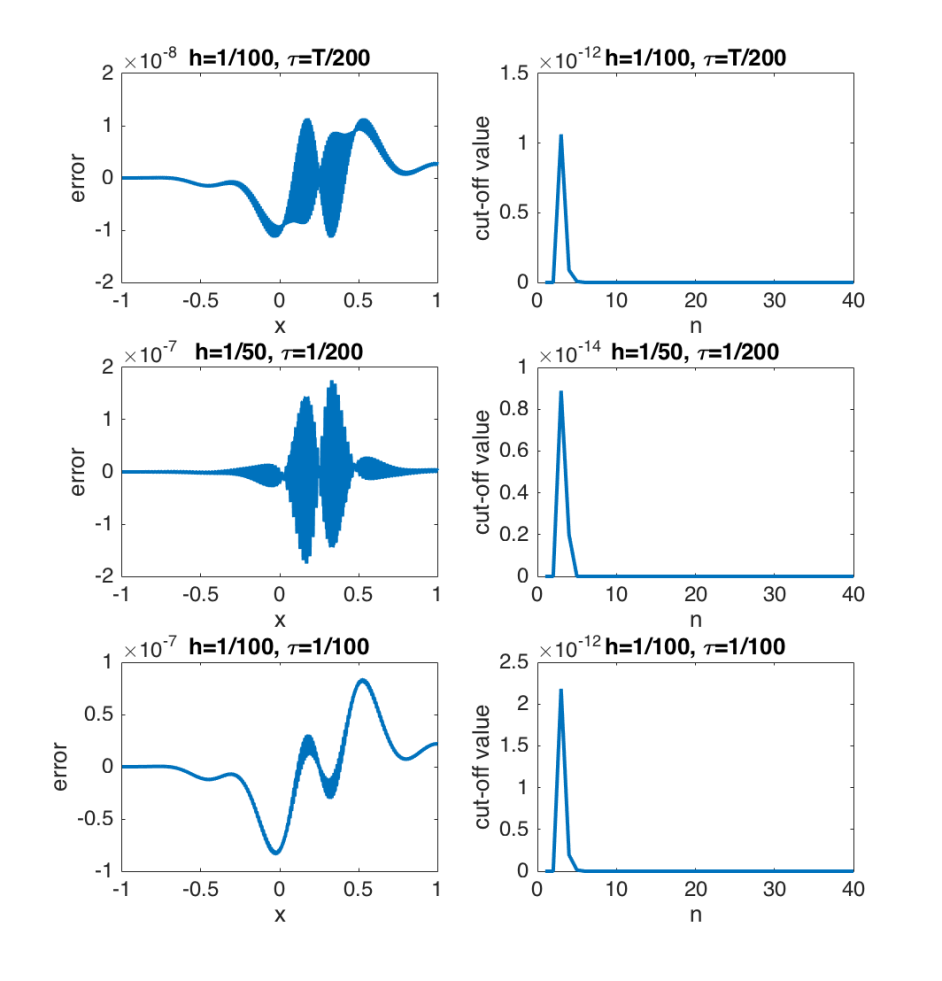
In Figure 4.1, we plot the maximal cut-off value at each step

$$\rho^{n}=\max_{0\leq j\leq Mr+1}|u_{h}^{n}(x_{j})-\hat{u}_{h}^{n}(x_{j})|$$

and the error of the numerical solution $e(x)=u^{N}_{h}(x)-u(x,T)$. Our numerical results show that the cut-off operation is active in the computation. Meanwhile, we observe that a coarse step mesh will result in a larger cut-off value, without affecting the convergence rate.

Fig. 1: Error at $T=0.01$ and maximal cut-off value at each time level.

(a) $m=1,\varepsilon=0.1,T=2,\tau=1/150$

(b) $m=2,\varepsilon=0.1,T=2,\tau=1/250$

Fig. 2: Left: solution profiles of numerical solutions of RK, cut-off RK and cut-off SAV-RK scheme. Middle: solution energy of cut-off RK and cut-off SAV-RK scheme. Right: cut-off values of cut-off RK and cut-off SAV-RK scheme.

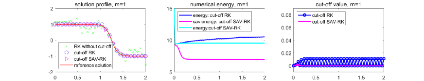
Finally, we test the numerical results in case of relatively large time steps, and compare the numerical solutions of extrapolated RK, cut-off RK (20)-(21), and cut-off SAV-RK schemes (30)-(32), with $r=1$, see Figure 2. Without the cut-off postprocessing, the numerical solutions of RK scheme significantly exceed the maximum bound, and present oscillating solution profiles. With the cut-off operation at each time step, the numerical solutions satisfy the maximum bound, and present reasonable solution profiles. However, numerical results show that the cut-off RK scheme might produce a solution with a obviously increasing and oscillating energy curve. This issue could be significantly improved by applying the cut-off SAV-RK method, whose solution satisfy the maximum bound and the numerical energy is more stable. Moreover, the numerical results show that the cut-off SAV-RK scheme will produce a more regular numerical solution and smaller cut-off values, compared with the cut-off RK scheme.

Appendix A

In this part, we sketch a proof for Lemma 7.

Proof.

We note that the second relation in equation (22) implies

$$u(t_{ni})-u(t_{n-1})-\tau\sum_{j=1}^{m}a_{ij}u_{t}^{nj}=\tau\sum_{j=1}^{m}a_{ij}(\dot{u}_{*}^{nj}-u_{t}(t_{nj}))+\eta_{ni}\quad\text{for}~{}~{}i=1,2,\dots,m.$$

Then we substitute the first relation of (22) and derive that for $i=1,2,\dots,m$

$$u(t_{ni})-u(t_{n-1})-\tau\sum_{j=1}^{m}a_{ij}u_{t}^{nj}=\tau\sum_{j=1}^{m}a_{ij}\Big{(}\sum_{\ell=1}^{k}L_{\ell}(t_{n-1}+c_{j}\tau)f(u(t_{n-\ell}))-f(t_{nj})\Big{)}+\eta_{ni}.$$

Define $\tilde{\eta}_{ni}$ as the left hand side of the above relation. Now we apply Taylor’s expansion at $t_{n-1}$ and use (19) to derive

$$\tilde{\eta}_{ni}= \sum_{l=1}^{m}\frac{\tau^{l}}{(l-1)!}\left(\frac{c_{i}^{l}}{l}-\sum_{j=1}^{m}a_{ij}c_{j}^{l-1}\right)u^{(\ell)}(t_{n})+\frac{1}{m!}\int_{t_{n-1}}^{t_{ni}}(t_{ni}-s)^{m}u^{(m+1)}(s)\mathrm{d}s$$

$$+\frac{\tau}{(m-1)!}\sum_{j=1}^{m}a_{ij}\int_{t_{n-1}}^{t_{nj}}(t_{nj}-s)^{m-1}u^{(m+1)}(s)\mathrm{d}s$$

$$=\frac{1}{m!}\int_{t_{n-1}}^{t_{ni}}(t_{n}-s)^{m}u^{(m+1)}(s)\mathrm{d}s+\frac{\tau}{(m-1)!}\sum_{j=1}^{m}a_{ij}\int_{t_{n-1}}^{t_{nj}}(t_{nj}-s)^{m-1}u^{(m+1)}(s)\mathrm{d}s$$

Then we obtain the estimate for $\tilde{\eta}_{ni}$, with $i=1,2,\dots,m$, that

$$\|\tilde{\eta}_{ni}\|_{H^{1}(\Omega)}\leqslant C\tau^{m+1}\|u^{(m+1)}\|_{C([t_{n-1},t_{n}];H^{1}(\Omega))}.$$

This together with the approximation property of Lagrange interpolation lead to

$$\|\eta_{ni}\|_{H^{1}(\Omega)}\leqslant C\Big{(}\tau^{k+1}\|f(u)\|_{C^{k}([t_{n-k},t_{n}];H^{1}(\Omega))}+\tau^{m+1}\|u\|_{C^{(m+1)}([t_{n-1},t_{n}];H^{1}(\Omega))}\Big{)}.$$

for $i=1,2,\dots,m$. Similarly, we have

$$u(t_{n})-u(t_{n-1})-\tau\sum_{i=1}^{m}b_{i}u_{t}^{ni}=\tau\sum_{i=1}^{m}b_{i}\Big{(}\sum_{\ell=1}^{k}L_{\ell}(t_{n-1}+c_{i}\tau)f(u(t_{n-\ell}))-f(t_{ni})\Big{)}+\eta_{n}.$$

Take the left hand side as $\tilde{\eta_{n}}$. Then Taylor expansion and (18) imply

$$\tilde{\eta}_{n}=\frac{1}{p!}\int_{t_{n-1}}^{t_{n}}(t_{n}-s)^{p}u^{(p+1)}(s)\mathrm{d}s+\frac{\tau}{(p-1)!}\sum_{i=1}^{m}b_{i}\int_{t_{n-1}}^{t_{ni}}(t_{ni}-s)^{p-1}u^{(p+1)}(s)\mathrm{d}s.$$

This together with the approximation property of Lagrange interpolation leads to

$$\|\eta_{ni}\|_{H^{1}(\Omega)}\leqslant C\Big{(}\tau^{k+1}\|f(u)\|_{C^{k}([t_{n-k},t_{n}];H^{1}(\Omega))}+\tau^{p+1}\|u\|_{C^{p+1}([t_{n-1},t_{n}];H^{1}(\Omega))}\Big{)}.$$

Using the choice that $k=\min(p,m+1)$, we derive the desired result. ∎

References

- [1] G. Akrivis, B. Li, and D. Li, Energy-decaying extrapolated RK-SAV methods for the Allen-Cahn and Cahn-Hilliard equations, SIAM J. Sci. Comput., 41 (2019), pp. A3703–A3727.
- [2] S. M. Allen and J. W. Cahn, A microscopic theory for anti-phase boundary motion and its application to anti-phase domain coarsening, Acta Metall, 27 (1979), pp. 1085–1095.
- [3] D. M. Anderson, G. B. McFadden, and A. A. Wheeler, Diffuse-interface methods in fluid mechanics, Annual review of fluid mechanics, 30 (1998), pp. 139–165.
- [4] P. Brenner, M. Crouzeix, and V. Thomée, Single-step methods for inhomogeneous linear differential equations in Banach space, RAIRO Anal. Numér., 16 (1982), pp. 5–26.
- [5] L.-Q. Chen, Phase-field models for microstructure evolution, Annual review of materials research, 32 (2002), pp. 113–140.
- [6] Q. Du, L. Ju, X. Li, and Z. Qiao, Maximum principle preserving exponential time differencing schemes for the nonlocal Allen-Cahn equation, SIAM J. Numer. Anal., 57 (2019), pp. 875–898.
- [7] , Maximum bound principles for a class of semilinear parabolic equations and exponential time differencing schemes, arXiv preprint: 2005.11465, to appear in SIAM Review, (2020).
- [8] B. L. Ehle, On Padé approximations to the exponential function and A-stable methods for the numerical solution of initial value problems, ProQuest LLC, Ann Arbor, MI, 1969. Thesis (Ph.D.)–University of Waterloo (Canada).
- [9] Y. Gong, J. Zhao, and Q. Wang, Arbitrarily high-order unconditionally energy stable schemes for thermodynamically consistent gradient flow models, SIAM J. Sci. Comput., 42 (2020), pp. B135–B156.
- [10] S. Gottlieb, D. I. Ketcheson, and C.-W. Shu, Strong stability preserving Runge-Kutta and multistep time discretizations, World Scientific Press, 2011.
- [11] S. Gottlieb and C.-W. Shu, Total variation diminishing runge-kutta schemes, Mathematics of computation, 67 (1998), pp. 73–85.
- [12] S. Gottlieb, C.-W. Shu, and E. Tadmor, Strong stability-preserving high-order time discretization methods, SIAM Rev., 43 (2001), pp. 89–112.
- [13] E. Hairer and G. Wanner, Solving ordinary differential equations. II, vol. 14 of Springer Series in Computational Mathematics, Springer-Verlag, Berlin, 2010. Stiff and differential-algebraic problems, Second revised edition, paperback.
- [14] L. Isherwood, Z. J. Grant, and S. Gottlieb, Strong stability preserving integrating factor Runge-Kutta methods, SIAM J. Numer. Anal., 56 (2018), pp. 3276–3307.
- [15] L. Ju, X. Li, Z. Qiao, and J. Yang, Maximum bound principle preserving integrating factor runge-kutta methods for semilinear parabolic equations, arXiv preprint arXiv:2010.12165, (2020).
- [16] B. Li, J. Yang, and Z. Zhou, Arbitrarily high-order exponential cut-off methods for preserving maximum principle of parabolic equations, SIAM J. Sci. Comput., 42 (2020), pp. A3957–A3978.
- [17] H. L. Liao, T. Tang, and T. Zhou, On energy stable, maximum-principle preserving, second order bdf scheme with variable steps for the allen-cahn equation, SIAM J. Numer. Math, 58 (2020), pp. 2294–2314.
- [18] H. Liu and H. Yu, Maximum-principle-satisfying third order discontinuous Galerkin schemes for Fokker-Planck equations, SIAM J. Sci. Comput., 36 (2014), pp. A2296–A2325.
- [19] X.-D. Liu and S. Osher, Nonoscillatory high order accurate self-similar maximum principle satisfying shock capturing schemes i, SIAM J. Numer. Anal., 33 (1996), pp. 760–779.
- [20] A. Ostermann and M. Roche, Runge-Kutta methods for partial differential equations and fractional orders of convergence, Math. Comp., 59 (1992), pp. 403–420.
- [21] J. Qiu and C.-W. Shu, Runge–Kutta discontinuous Galerkin method using WENO limiters, SIAM J. Sci. Comput., 26 (2005), pp. 907–929.
- [22] A. Quarteroni, R. Sacco, and F. Saleri, Numerical mathematics, vol. 37 of Texts in Applied Mathematics, Springer-Verlag, New York, 2000.
- [23] J. Shen, T. Tang, and J. Yang, On the maximum principle preserving schemes for the generalized Allen-Cahn equation, Commun. Math. Sci., 14 (2016), pp. 1517–1534.
- [24] J. Shen and J. Xu, Convergence and error analysis for the scalar auxiliary variable (SAV) schemes to gradient flows, SIAM J. Numer. Anal., 56 (2018), pp. 2895–2912.
- [25] J. Shen, J. Xu, and J. Yang, The scalar auxiliary variable (sav) approach for gradient flows, Journal of Computational Physics, 353 (2018), pp. 407–416.
- [26] J. Shen, J. Xu, and J. Yang, A new class of efficient and robust energy stable schemes for gradient flows, SIAM Review, 61 (2019), pp. 474–506.
- [27] T. Tang and J. Yang, Implicit-explicit scheme for the Allen-Cahn equation preserves the maximum principle, J. Comput. Math., 34 (2016), pp. 471–481.
- [28] V. Thomée, Galerkin Finite Element Methods for Parabolic Problems, Springer-Verlag, Berlin, second ed., 2006.
- [29] J. J. W. van der Vegt, Y. Xia, and Y. Xu, Positivity preserving limiters for time-implicit higher order accurate discontinuous Galerkin discretizations, SIAM J. Sci. Comput., 41 (2019), pp. A2037–A2063.
- [30] Z. Xu, Parametrized maximum principle preserving flux limiters for high order schemes solving hyperbolic conservation laws: one-dimensional scalar problem, Math. Comp., 83 (2014), pp. 2213–2238.
- [31] P. Yue, J. J. Feng, C. Liu, and J. Shen, A diffuse-interface method for simulating two-phase flows of complex fluids, Journal of Fluid Mechanics, 515 (2004), p. 293.
- [32] X. Zhang and C.-W. Shu, On maximum-principle-satisfying high order schemes for scalar conservation laws, J. Comput. Phys., 229 (2010), pp. 3091–3120.