The numerical range of a periodic tridiagonal operator reduces to the numerical range of a finite matrix

Abstract.

In this paper we show that the closure of the numerical range of an $n+1$-periodic tridiagonal operator is equal to the numerical range of a $2(n+1)\times 2(n+1)$ complex matrix.

Introduction

Consider $\mathcal{A}$ to be a finite set of complex numbers and let $a=(a_{i})_{i\in{\mathbb{Z}}}$ be a biinfinite sequence in the total shift space $\mathcal{A}^{\mathbb{Z}}$. In [13], the tridiagonal operator $A_{a}\colon\ell^{2}({\mathbb{Z}})\to\ell^{2}({\mathbb{Z}})$ associated to $a$ is defined as

(1) $$A_{a}=\begin{pmatrix}\ddots&\ddots&&&&&\\ \ddots&0&1&&&&\\ &a_{-2}&0&1&&&\\ &&a_{-1}&\framebox[11.38092pt][l]{0}&1&&\\ &&&a_{0}&0&1&\\ &&&&a_{1}&0&\ddots\\ &&&&&\ddots&\ddots\end{pmatrix}$$

where the square marks the matrix entry at $(0,0)$. In the particular case of the alphabet $\mathcal{A}=\{-1,1\}$, the corresponding operator $A_{a}$ is related to the so called “hopping sign model” introduced in [7] and subsequently studied in many other works, such as [1, 2, 3, 4, 5, 6, 9, 10, 13], just to name a few. On the other hand, when the alphabet is $\mathcal{A}=\{0,1\}$ some results for computing the numerical range of $A_{a}$ are presented in [13, 14]. In particular, work in [14] addresses the case when $a$ is an $n+1$-periodic sequence. Relying on the fact that the closure of the numerical range of $A_{a}$ may be written as the closure of the convex hull of an uncountable union of numerical ranges of certain matrices, in [14] the closure of the numerical range of the 2-periodic case is computed by substituting such uncountable union of numerical ranges by the convex hull of the union of the numerical ranges of just two $2\times 2$ matrices. In this work, we further contribute to the study of the numerical range of $A_{a}$ when $a$ is an $n+1$ periodic biinfinite sequence.

Instead of working with the operators $A_{a}$, we work with the more general tridiagonal operators $T=T(a,b,c)$ defined in Section 2, since, as can be seen in [14], the computation of the closure of the numerical range of $A_{a}$ is a particular case of that of $T$. Using a result of Plaumann and Vinzant [20], we show that the closure of the numerical range of the $n+1$ periodic tridiagonal operator $T$ is the numerical range of a $2(n+1)\times 2(n+1)$ matrix (cf. Theorem 2.6).

We divide this work in two sections. In Section 1 we briefly introduce the notation and terminologies needed in the rest of the paper. In Section 2 we develop the required machinery, first by computing the Kippenhahn polynomial of the symbol of $n+1$ periodc tridiagonal operatos $T$ on $\ell^{2}({\mathbb{N}}_{0})$ and then by combining our computations with results of Plaumann and Vizant. We will conclude that the closure of the numerical range of $T$ is equal to the numerical range of a $2(n+1)\times 2(n+1)$ matrix $A$. Furthermore, we provide some examples where $A$ can be explicitly computed and we show that the size of $A$ is optimal.

1. Preliminaries

In this section we introduce the notation required which will be needed in the following sections. As usual, the symbols ${\mathbb{N}}$, ${\mathbb{N}}_{0}$, ${\mathbb{Z}}$, ${\mathbb{R}}$ and ${\mathbb{C}}$ will denote the set of positive integers, the sets of nonnegative integers, the set of integers, the set of real numbers and the set of complex numbers, respectively.

For a given $n\in{\mathbb{N}}$, let $a$, $b$ and $c$ be $(n+1)$-periodic infinite sequences in $\mathcal{A}^{{\mathbb{N}}_{0}}$. We will denote by $T=T(a,b,c)$ the $(n+1)$-periodic tridiagonal operator on $\ell^{2}({\mathbb{N}}_{0})$ given by

$$T=\setcounter{MaxMatrixCols}{11}\begin{pmatrix}b_{0}&c_{0}&&&&&&&&\\ a_{1}&b_{1}&c_{1}&&&&&&&\\ &a_{2}&b_{2}&c_{2}&&&&&&\\ &&\ddots&\ddots&\ddots&&&&&\\ &&&a_{n}&b_{n}&c_{n}&&&&\\ &&&&a_{0}&b_{0}&c_{0}&&&\\ &&&&&\ddots&\ddots&\ddots&&\\ &&&&&&a_{n-1}&b_{n-1}&c_{n-1}&\\ &&&&&&&a_{n}&b_{n}&c_{n}&\\ &&&&&&&&\ddots&\ddots&\ddots\end{pmatrix}.$$

We should observe that $T$ is a bounded operator since the sum of the moduli of the entries in each column (and in each row) is uniformly bounded (see, e.g., [16, Example 2.3]). The biinfinite matrix $A_{a}$ is also a bounded operator, as long as the biinfinite sequence $a$ arises from a finite alphabet.

If $n>1$, for each $\phi\in[0,2\pi)$, following [1, 14] we define the symbol of $T$, as the following $(n+1)\times(n+1)$ matrix

(2) $$T_{\phi}=\begin{pmatrix}b_{0}&c_{0}&0&&&0&a_{0}e^{-i\phi}\\ a_{1}&b_{1}&c_{1}&0&&&0\\ 0&a_{2}&b_{2}&c_{2}&0&&\\ &\ddots&\ddots&\ddots&\ddots&\ddots&\\ &&0&a_{n-2}&b_{n-2}&c_{n-2}&0\\ 0&&&0&a_{n-1}&b_{n-1}&c_{n-1}\\ c_{n}e^{i\phi}&0&&&0&a_{n}&b_{n}\end{pmatrix};$$

while the symbol of $T$ for $n=1$ is the $2\times 2$ matrix

(3) $$T_{\phi}=\begin{pmatrix}b_{0}&c_{0}+a_{0}e^{-i\phi}\\ a_{1}+c_{1}e^{i\phi}&b_{1}\end{pmatrix}.$$

Recall that given a Hilbert space $\mathcal{H}$ and a bounded operator $A$ on it, the numerical range is defined as the set

$$W(A)=\{\left<Ax,x\right>\,:\,\|x\|=1\}.$$

The Toeplitz-Haussdorf Theorem establishes that $W(A)$ is a bounded convex subset of ${\mathbb{C}}$ (closed, if the Hilbert space is finite dimensional) and hence the closure of the numerical range can be seen as the intersection of the closed half-spaces containing the numerical range.

Kippenhahn [17] (see also [18]) characterized two vertical support lines of $W(A)$ for a given $n\times n$ matrix as $\mathrm{Re}(z)=\lambda_{1}(A)$ and $\mathrm{Re}(z)=\lambda_{n}(A)$, where $\lambda_{1}(A)$ and $\lambda_{n}(A)$ are the respective largest and least eigenvalues of $\mathrm{Re}(A)$ (recall that $\mathrm{Re}(A):=\frac{1}{2}(A+A^{*})$ and $\mathrm{Im}(A):=\frac{1}{2i}(A-A^{*})$). In fact, if $\alpha\in W(A)$ then $\lambda_{n}(A)\leq\mathrm{Re}(\alpha)\leq\lambda_{1}(A)$ (and the equalities hold for some points $\alpha_{1},\alpha_{2}\in W(A)$). Since $e^{i\theta}W(A)=W(e^{i\theta}A)$ for each $\theta\in[0,2\pi)$, it follows that if $\alpha\in W(A)$, then $e^{-i\theta}\alpha\in W(e^{-i\theta}A)$ and hence $\mathrm{Re}(e^{-i\theta}\alpha)\leq\lambda_{1}(e^{-i\theta}A)$. It follows that the lines $\mathrm{Re}(e^{-i\theta}z)=\lambda_{1}(e^{-i\theta}A)$ are support lines of $W(A)$. Hence the convex set $W(A)$ is uniquely determined by the numbers $\lambda_{1}(e^{-i\theta}A)$, as $\theta$ varies on the interval $[0,2\pi)$; i.e. $W(A)$ is determined by the largest eigenvalue of $\mathrm{Re}(e^{-i\theta}A)$, which equals $\cos(\theta)\mathrm{Re}(A)+\sin(\theta)\mathrm{Im}(A)$. Thus the numerical range is determined by the largest roots of the family of characteristic polynomials

$$\det(tI_{n}-\cos(\theta)\mathrm{Re}(A)-\sin(\theta)\mathrm{Im}(A)).$$

The homogeneous polynomial $F_{A}(t,x,y)=\det(tI_{n}+x\mathrm{Re}(A)+y\mathrm{Im}(A))$ is called the Kippenhahn polynomial of the matrix $A$. It clearly follows that two matrices have the same numerical range if their Kippenhahn polynomials coincide. Furthermore,

$$\max\{t\in{\mathbb{R}}\,:\,F_{A}(t,-\cos(\theta),-\sin(\theta))=0\}=\max\{\mathrm{Re}(e^{-i\theta}z)\,:\,z\in W(A)\}$$

for each $\theta\in[0,2\pi)$.

2. The Kippenhahn polynomial of the symbol $T_{\phi}$

In this section, after some preliminary work, we show that the closure of the numerical range of a $n+1$-periodic tridiagonal operator $T$ is the numerical range of a $2(n+1)\times 2(n+1)$ matrix.

We will need the following lemma.

Lemma 2.1.

Consider the $(n+1)\times(n+1)$ “almost tridiagonal” matrix

$$\Lambda=\begin{pmatrix}\lambda_{1,1}&\lambda_{1,2}&0&0&\dots&0&0&\lambda_{1,n+1}\\ \lambda_{2,1}&\lambda_{2,2}&\lambda_{2,3}&0&\dots&0&0&0\\ 0&\lambda_{3,2}&\lambda_{3,3}&\lambda_{3,4}&\dots&0&0&0\\ 0&0&\lambda_{4,3}&\lambda_{4,4}&\dots&0&0&0\\ \vdots&\vdots&\vdots&\vdots&\ddots&\vdots&\vdots&\vdots\\ 0&0&0&0&\dots&\lambda_{n-1,n-1}&\lambda_{n-1,n}&0\\ 0&0&0&0&\dots&\lambda_{n,n-1}&\lambda_{n,n}&\lambda_{n,n+1}\\ \lambda_{n+1,1}&0&0&0&\dots&0&\lambda_{n+1,n}&\lambda_{n+1,n+1}\end{pmatrix},$$

where every $\lambda_{i,j}\in{\mathbb{C}}$. Then, $\det(\Lambda)$ equals

$$\begin{split}&\det\begin{pmatrix}\lambda_{1,1}&\lambda_{1,2}&0&\dots&0&0\\ \lambda_{2,1}&\lambda_{2,2}&\lambda_{2,3}&\dots&0&0\\ 0&\lambda_{3,2}&\lambda_{3,3}&\dots&0&0\\ \vdots&\vdots&\vdots&\ddots&\vdots&\vdots\\ 0&0&0&\dots&\lambda_{n-1,n}&0\\ 0&0&0&\dots&\lambda_{n,n}&\lambda_{n,n+1}\\ 0&0&0&\dots&\lambda_{n+1,n}&\lambda_{n+1,n+1}\end{pmatrix}-\lambda_{1,n+1}\lambda_{n+1,1}\det\begin{pmatrix}\lambda_{2,2}&\lambda_{2,3}&\dots&0&0\\ \lambda_{3,2}&\lambda_{3,3}&\dots&0&0\\ \vdots&\vdots&\ddots&\vdots&\vdots\\ 0&0&\dots&\lambda_{n-1,n-1}&\lambda_{n-1,n}\\ 0&0&\dots&\lambda_{n,n-1}&\lambda_{n,n}\end{pmatrix}\\ \\ &+(-1)^{n}\lambda_{n+1,1}\lambda_{1,2}\lambda_{2,3}\cdots\lambda_{n-1,n}\lambda_{n,n+1}+(-1)^{n}\lambda_{1,n+1}\lambda_{2,1}\lambda_{3,2}\cdots\lambda_{n,n-1}\lambda_{n+1,n}.\end{split}$$

Proof.

This follows by a long (but straightforward) application of the multilinearity of the determinant function and the Laplace Expansion Theorem. ∎

Let us set the following notation for the rest of this paper. For $0\leq j<n$ we define

$$\alpha_{j}=\frac{c_{j}+\overline{a_{j+1}}}{2},\quad\gamma_{j}=\frac{c_{j}-\overline{a_{j+1}}}{2i}$$

and

$$\alpha_{n}=\frac{a_{0}+\overline{c_{n}}}{2},\quad\gamma_{n}=\frac{a_{0}-\overline{c_{n}}}{2i}.$$

We now find an expression for the Kippenhahn polynomial $F_{T_{\phi}}$ of the symbol matrix $T_{\phi}$ of an arbitrary $n+1$-periodic tridiagonal matrix $T$ acting on $\ell^{2}({\mathbb{N}}_{0})$, involving the determinants of some tridiagonal matrices. This expression will be useful in what follows.

Proposition 2.2.

Let $n\in{\mathbb{N}}$. Consider the symbol $T_{\phi}$, that is, the $(n+1)\times(n+1)$ matrix defined as in (2) for $n\geq 2$ and as in (3) for $n=1$. Then the Kippenhahn polynomial of $T_{\phi}$ is equal to

$$F_{T_{\phi}}(t,x,y)={} G_{n}(t,x,y)-|\alpha_{n}x+\gamma_{n}y|^{2}H_{n}(t,x,y)+2(-1)^{n}\ \mathrm{Re}\left(\left(\overline{\alpha_{n}}x+\overline{\gamma_{n}}y\right){\prod_{j=0}^{n-1}}(\alpha_{j}x+\gamma_{j}y)\right)\cos\phi$$

$$-2(-1)^{n}\ \mathrm{Im}\left(\left(\overline{\alpha_{n}}x+\overline{\gamma_{n}}y\right){\prod_{j=0}^{n-1}}(\alpha_{j}x+\gamma_{j}y)\right)\sin\phi,$$

where $G_{n}(t,x,y)$ is the determinant of the tridiagonal $(n+1)\times(n+1)$ matrix

$$\begin{pmatrix}\lambda_{1,1}&\lambda_{1,2}&0&0&\ldots&0&0\\ \lambda_{2,1}&\lambda_{2,2}&\lambda_{2,3}&0&\cdots&0&0\\ 0&\lambda_{3,2}&\lambda_{3,3}&\lambda_{3,3}&\cdots&0&0\\ 0&0&\lambda_{4,3}&\lambda_{4,4}&\cdots&0&0\\ \vdots&\vdots&\vdots&\vdots&&\vdots&\vdots\\ 0&0&0&0&\cdots&\lambda_{n,n}&\lambda_{n,n+1}\\ 0&0&0&0&\cdots&\lambda_{n+1,n}&\lambda_{n+1,n+1}\end{pmatrix},$$

and, where we set $H_{n}(t,x,y)=1$ when $n=1$, and, for $n\geq 2$, we set $H_{n}(t,x,y)$ to be the determinant of $(n-1)\times(n-1)$ tridiagonal matrix

$$\begin{pmatrix}\lambda_{2,2}&\lambda_{2,3}&0&\cdots&0&0\\ \lambda_{3,2}&\lambda_{3,3}&\lambda_{3,4}&\cdots&0&0\\ 0&\lambda_{4,3}&\lambda_{4,4}&\cdots&0&0\\ \vdots&\vdots&\vdots&&\vdots&\vdots\\ 0&0&0&\cdots&\lambda_{n-1,n-1}&\lambda_{n-1,n}\\ 0&0&0&\cdots&\lambda_{n,n-1}&\lambda_{n,n}\end{pmatrix}.$$

Here we have set, for $1\leq j\leq n+1$,

$$\lambda_{j,j}=t+\mathrm{Re}(b_{j-1})x+\mathrm{Im}(b_{j-1})y,$$

and for $1\leq j\leq n$,

$$\lambda_{j,j+1}=\alpha_{j-1}x+\gamma_{j-i}y\quad\text{ and}\quad\lambda_{j+1,j}=\overline{\alpha_{j-1}}x+\overline{\gamma_{j-1}}y.$$

Proof.

We divide the proof in two cases. For $n+1=2$, by computing the real and imaginary parts of the matrix $T_{\phi}$ in (3), we obtain that the $2\times 2$ matrix $tI_{2}+x\mathrm{Re}(T_{\phi})+y\mathrm{Im}(T_{\phi})$ is given by

$$\begin{pmatrix}t+\mathrm{Re}(b_{0})x+\mathrm{Im}(b_{0})y&\alpha_{0}x+\gamma_{0}y+(\alpha_{1}x+\gamma_{1}y)e^{-i\phi}\cr(\overline{\alpha_{0}}x+\overline{\gamma_{0}}y)+(\overline{\alpha_{1}}x+\overline{\gamma_{1}}y)e^{i\phi}&t+\mathrm{Re}(b_{1})x+\mathrm{Im}(b_{1})y\end{pmatrix},$$

where $\alpha_{0}$, $\alpha_{1}$, $\gamma_{0}$ and $\gamma_{1}$ are as defined above. The determinant of this matrix can be simplified to

$$F_{T_{\phi}}(t,x,y)={} (t+\mathrm{Re}(b_{0})x+\mathrm{Im}(b_{0})y)(t+\mathrm{Re}(b_{1})x+\mathrm{Im}(b_{1})y)-|\alpha_{0}x+\gamma_{0}y|^{2}-|\alpha_{1}x+\gamma_{1}y|^{2}$$

$$\quad-2\mathrm{Re}\left((\alpha_{0}x+\gamma_{0}y)(\overline{\alpha_{1}}x+\overline{\gamma_{1}}y)e^{i\phi}\right)$$

$$={} (t+\mathrm{Re}(b_{0})x+\mathrm{Im}(b_{0})y)(t+\mathrm{Re}(b_{1})x+\mathrm{Im}(b_{1})y)-|\alpha_{0}x+\gamma_{0}y|^{2}-|\alpha_{1}x+\gamma_{1}y|^{2}$$

$$\quad-2\mathrm{Re}\left((\alpha_{0}x+\gamma_{0}y)(\overline{\alpha_{1}}x+\overline{\gamma_{1}}y)\right)\cos\phi+2\mathrm{Im}\left((\alpha_{0}x+\gamma_{0}y)(\overline{\alpha_{1}}x+\overline{\gamma_{1}}y)\right)\sin\phi$$

$$={} G_{1}(t,x,y)-|\alpha_{1}x+\gamma_{1}t|^{2}H_{1}(t,x,y)$$

$$\quad-2\mathrm{Re}\left((\alpha_{0}x+\gamma_{0}y)(\overline{\alpha_{1}}x+\overline{\gamma_{1}}y)\right)\cos\phi+2\mathrm{Im}\left((\alpha_{0}x+\gamma_{0}y)(\overline{\alpha_{1}}x+\overline{\gamma_{1}}y)\right)\sin\phi,$$

as desired.

Now, for the case $n+1\geq 3$, by computing the real and imaginary parts of the matrix $T_{\phi}$ in (2), we can observe that $tI_{n+1}+x\mathrm{Re}(T_{\phi})+y\mathrm{Im}(T_{\phi})$ is the matrix

$$\begin{pmatrix}\lambda_{1,1}&\lambda_{1,2}&0&0&\ldots&0&\lambda_{1,n+1}\\ \lambda_{2,1}&\lambda_{2,2}&\lambda_{2,3}&0&\cdots&0&0\\ 0&\lambda_{3,2}&\lambda_{3,3}&\lambda_{3,3}&\cdots&0&0\\ 0&0&\lambda_{4,3}&\lambda_{4,4}&\cdots&0&0\\ \vdots&\vdots&\vdots&\vdots&&\vdots&\vdots\\ 0&0&0&0&\cdots&\lambda_{n,n}&\lambda_{n,n+1}\\ \lambda_{n+1,1}&0&0&0&\cdots&\lambda_{n+1,n}&\lambda_{n+1,n+1}\end{pmatrix},$$

where we have now set

$$\lambda_{1,n+1}=(\alpha_{n}x+\gamma_{n}y)e^{-i\phi}\quad\text{and}\quad\lambda_{n+1,1}=(\overline{\alpha_{n}}x+\overline{\gamma_{n}}y)e^{i\phi}.$$

The above matrix is tridiagonal, except for the upper-right and bottom-left corners.

We can compute the determinant of the matrix polynomial $tI_{n+1}+x\mathrm{Re}(T_{\phi})+y\mathrm{Im}(T_{\phi})$ by using Lemma 2.1 obtaining

$$F_{T_{\phi}}(t,x,y)={} \det(tI_{n+1}+x\mathrm{Re}(T_{\phi})+y\mathrm{Im}(T_{\phi}))$$

$$={} G_{n}(t,x,y)-|\alpha_{n}x+\gamma_{n}y|^{2}\ H_{n}(t,x,y)$$

$$+(-1)^{n}(\overline{\alpha_{n}}x+\overline{\gamma_{n}}y)\prod_{j=0}^{n-1}(\alpha_{j}x+\gamma_{j}y)e^{i\phi}+(-1)^{n}(\alpha_{n}x+\gamma_{n}y)\prod_{j=0}^{n-1}(\overline{\alpha_{j}}x+\overline{\gamma_{j}}y)e^{-i\phi}$$

$$={} G_{n}(t,x,y)-|\alpha_{n}x+\gamma_{n}y|^{2}\ H_{n}(t,x,y)+2(-1)^{n}\mathrm{Re}\left((\overline{\alpha_{n}}x+\overline{\gamma_{n}}y)\prod_{j=0}^{n-1}(\alpha_{j}x+\gamma_{j}y)e^{i\phi}\right).$$

Computing the real part of the last term above, we obtain the equation

$$F_{T_{\phi}}(t,x,y)={} G_{n}(t,x,y)-|\alpha_{n}x+\gamma_{n}y|^{2}H_{n}(t,x,y)+2(-1)^{n}\ \mathrm{Re}\left(\left(\overline{\alpha_{n}}x+\overline{\gamma_{n}}y\right){\prod_{j=0}^{n-1}}(\alpha_{j}x+\gamma_{j}y)\right)\cos\phi$$

$$-2(-1)^{n}\ \mathrm{Im}\left(\left(\overline{\alpha_{n}}x+\overline{\gamma_{n}}y\right){\prod_{j=0}^{n-1}}(\alpha_{j}x+\gamma_{j}y)\right)\sin\phi,$$

which completes the proof. ∎

For every $n\in{\mathbb{N}}$ and for a fixed point $(x,y)\in{\mathbb{R}}^{2}$, the angle $\phi\in[0,2\pi)$ is involved only in the constant term (with respect to the variable $t$) of the polynomial $F_{T_{\phi}}(t,x,y)$. Furthermore, for every $(x,y)\in{\mathbb{R}}^{2}$ and for every $\phi\in[0,2\pi)$, the polynomial $F_{T_{\phi}}(t,x,y)$, seen as a polynomial in $t$, has $n+1$ real roots, counting multiplicities, as it is the characteristic polynomial of the Hermitian matrix $-x\mathrm{Re}(T_{\phi})-y\mathrm{Im}(T_{\phi})$. The following lemma will be useful later when applied to the polynomial $F_{T_{\phi}}$.

Lemma 2.3.

Let $F(t:\phi)$ be a family of polynomials in ${\mathbb{R}}[t]$ given by the expression

$$F(t:\phi)=t^{n+1}+p_{n}t^{n}+\ldots+p_{1}t+p_{0}-u\cos\phi-v\sin\phi,$$

where $\phi\in[0,2\pi)$. Assume that the polynomial $F(t:\phi)$ has $n+1$ real roots counting multiplicities for any angle $\phi\in[0,2\pi)$. Let $\phi_{0}$, $\phi_{1}\in[0,2\pi)$ be such that

$$u\cos\phi_{0}+v\sin\phi_{0}=-\sqrt{u^{2}+v^{2}}\quad\text{ and }\quad u\cos\phi_{1}+v\sin\phi_{1}=\sqrt{u^{2}+v^{2}}.$$

Then

$$\max\left\{\max\left\{t\in{\mathbb{R}}\,:\,F(t:\phi)=0\right\}:0\leq\phi<2\pi\right\}=\max\left\{t\in{\mathbb{R}}\,:\,F(t:\phi_{1})=0\right\},$$

and

$$\min\left\{\max\left\{t\in{\mathbb{R}}\,:\,F(t:\phi)=0\right\}:0\leq\phi<2\pi\right\}=\max\left\{t\in{\mathbb{R}}\,:\,F(t:\phi_{0})=0\right\}.$$

Proof.

Define $p(t)$ as

$$p(t)=t^{n+1}+p_{n}t^{n}+\ldots+p_{1}t+p_{0}.$$

Observe that, by assumption, the equation

$$p(t)=u\cos\phi+v\sin\phi$$

has $n+1$ real solutions (counting multiplicities) for every $\phi\in[0,2\pi)$. For some $\phi\in[0,2\pi)$, we have $u\cos\phi+v\sin\phi=0$, and hence $p$ has $n+1$ real roots (counting multiplicities) and the derivative of $p$ has $n$ real roots (counting multiplicities). Let $r_{0}$ be the largest root of $p^{\prime}(t)$. Hence, $p$ is increasing on the interval $[r_{0},\infty)$ and the equations

$$p(t)=u\cos\phi+v\sin\phi$$

have a unique solution on the interval $[r_{0},\infty)$.

Observe that for every $\phi\in[0,2\pi)$

$$-\sqrt{u^{2}+v^{2}}\leq u\cos\phi+v\sin\phi\leq\sqrt{u^{2}+v^{2}};$$

equality occurs on the left-hand-side inequality at $\phi_{0}$ while equality occurs on the right-hand-side inequality at $\phi_{1}$.

For each $\phi\in[0,2\pi)$, consider the number

$$\max\{t\in{\mathbb{R}}\,:\,p(t)=u\cos\phi+v\sin\phi\}.$$

Since the function $p$ is increasing on $[r_{0},\infty)$, the largest of these numbers, when $\phi$ varies, occurs when $t$ is the largest solution of the equation

$$p(t)=\sqrt{u^{2}+v^{2}}.$$

Hence we have

$$\max\left\{\max\left\{t\in{\mathbb{R}}\,:\,F(t,\phi)=0\right\}:0\leq\phi<2\pi\right\}=\max\left\{t\in{\mathbb{R}}\,:\,F(t,\phi_{1})=0\right\}.$$

Analogously, the smallest, when $\phi$ varies in $[0,2\pi)$, among the largest solutions $t$ of the equations

$$p(t)=u\cos\phi+v\sin\phi,$$

occurs when $t$ is the largest solution of the equation

$$p(t)=-\sqrt{u^{2}+v^{2}}.$$

Hence we have

$$\min\left\{\max\left\{t\in{\mathbb{R}}\,:\,F(t,\phi)=0\right\}:0\leq\phi<2\pi\right\}=\max\left\{t\in{\mathbb{R}}\,:\,F(t,\phi_{0})=0\right\}.\qed$$

In Theorem 2.7, we will show that the closure of the numerical range of $T$ is the numerical range of a single matrix. One of the key steps in the proof of said theorem will be to use the following proposition, which computes the closure of the numerical range of $T$ by using a single homogeneous polynomial, instead of the uncountable number of Kippenhahn polynomials of the symbols $T_{\phi}$, which Theorem 2.8 in [14] would suggest: this is achieved by getting rid of the parameter $\phi$ in the expression of the Kippenhahn polynomial of the symbol $T_{\phi}$ in Proposition 2.2.

Proposition 2.4.

Let $n\in{\mathbb{N}}$. Suppose that $T(a,b,c)$ is an $n+1$-periodic tridiagonal operator acting on $\ell^{2}({\mathbb{N}}_{0})$. Let $G_{n}$ and $H_{n}$ be as in Proposition 2.2 and let $P$ be the real homogeneous polynomial of degree $2(n+1)$ given by

$$P(t,x,y)=\left(G_{n}(t,x,y)-|\alpha_{n}x+\gamma_{n}y|^{2}H_{n}(t,x,y)\right)^{2}-4\prod_{j=0}^{n}\left|\alpha_{j}x+\gamma_{j}y\right|^{2}.$$

Then $P(t,0,0)=t^{2(n+1)}$ and

$$\sup\left\{\mathrm{Re}(e^{-i\theta}z)\colon\right.\bigl{.}z\in W\left(T(a,b,c)\right)\bigr{\}}=\max\{t\in{\mathbb{R}}\colon P(t,-\cos\theta,-\sin\theta)=0\},$$

for each $\theta\in[0,2\pi)$.

Proof.

It is trivial to check that $P(t,0,0)=t^{2(n+1)}$. Now, let $F(t:\phi)=F_{T_{\phi}}(t,x,y)$, where we know by Proposition 2.2 that

$$F_{T_{\phi}}(t,x,y)=G_{n}(t,x,y)-|\alpha_{n}x+\gamma_{n}y|^{2}H_{n}(t,x,y)-u\cos\phi-v\sin\phi,$$

where

$$u=-2(-1)^{n}\ \mathrm{Re}\left(\left(\overline{\alpha_{n}}x+\overline{\gamma_{n}}y\right){\prod_{j=0}^{n-1}}(\alpha_{j}x+\gamma_{j}y)\right)$$

and

$$v=2(-1)^{n}\ \mathrm{Im}\left(\left(\overline{\alpha_{n}}x+\overline{\gamma_{n}}y\right){\prod_{j=0}^{n-1}}(\alpha_{j}x+\gamma_{j}y)\right).$$

Notice that

$$u^{2}+v^{2}={} 4\mathrm{Re}^{2}\left(\left(\overline{\alpha_{n}}x+\overline{\gamma_{n}}y\right){\prod_{j=0}^{n-1}}(\alpha_{j}x+\gamma_{j}y)\right)+4\mathrm{Im}^{2}\left(\left(\overline{\alpha_{n}}x+\overline{\gamma_{n}}y\right){\prod_{j=0}^{n-1}}(\alpha_{j}x+\gamma_{j}y)\right)$$

$$={} 4\left|\left(\overline{\alpha_{n}}x+\overline{\gamma_{n}}y\right){\prod_{j=0}^{n-1}}(\alpha_{j}x+\gamma_{j}y)\right|^{2}$$

$$= {}4\prod_{j=0}^{n}\left|\alpha_{j}x+\gamma_{j}y\right|^{2}.$$

The polynomial $F(t:\phi)$ has the form outlined in Lemma 2.3 and, as was mentioned before Lemma 2.3, it has $n+1$ real roots, counting multiplicities. Hence, by Lemma 2.3, for $\phi_{0}$ and $\phi_{1}$ satisfying

$$u\cos(\phi_{0})+v\sin(\phi_{0})=-\sqrt{u^{2}+v^{2}},\qquad u\cos(\phi_{1})+v\sin(\phi_{1})=\sqrt{u^{2}+v^{2}},$$

we have that

$$\max\left\{\max\left\{t:F(t:\phi)=0\right\}:0\leq\phi<2\pi\right\}=\max\left\{t:F(t:\phi_{1})=0\right\},$$

and

$$\min\left\{\max\left\{t:F(t:\phi)=0\right\}:0\leq\phi<2\pi\right\}=\max\left\{t:F(t:\phi_{0})=0\right\}.$$

Notice that

$$F(t:\phi_{0})\cdot F(t:\phi_{1})={} \left(G_{n}(t,x,y)-|\alpha_{n}x+\gamma_{n}y|^{2}H_{n}(t,x,y)-\left(u\cos(\phi_{0})+v\sin(\phi_{0})\right)\right)$$

$$\cdot\left(G_{n}(t,x,y)-|\alpha_{n}x+\gamma_{n}y|^{2}H_{n}(t,x,y)-\left(u\cos(\phi_{1})+v\sin(\phi_{1})\right)\right)$$

$$={} \left(G_{n}(t,x,y)-|\alpha_{n}x+\gamma_{n}y|^{2}H_{n}(t,x,y)\right)^{2}-\left(\sqrt{u^{2}+v^{2}}\right)^{2}$$

$$={} \left(G_{n}(t,x,y)-|\alpha_{n}x+\gamma_{n}y|^{2}H_{n}(t,x,y)\right)^{2}-(u^{2}+v^{2})$$

$$={} P(t,x,y).$$

We also have, for each $\theta\in[0,2\pi)$, that

(4) $$\begin{split}\max\{t\in{\mathbb{R}}\colon F_{T_{\phi}}(t,-\cos\theta,&-\sin\theta)=0,\ 0\leq\phi<2\pi\}\\ ={}&\max\left\{\max\left\{t\in{\mathbb{R}}\colon F_{T_{\phi}}(t,-\cos\theta,-\sin\theta)=0\right\}\colon\ 0\leq\phi<2\pi\right\}\\ ={}&\max\left\{t\in{\mathbb{R}}\colon F_{T_{\phi_{1}}}(t,-\cos\theta,-\sin\theta)=0\right\}\\ ={}&\max\{t\in{\mathbb{R}}\colon P(t,-\cos\theta,-\sin\theta)=0\}.\end{split}$$

The last equality follows since the roots of $P(t,-\cos\theta,-\sin\theta)$ are those of $F(t:\phi_{1})=F_{T_{\phi_{1}}}(t,-\cos\theta,-\sin\theta)$ and $F(t:\phi_{0})=F_{T_{\phi_{0}}}(t,-\cos\theta,-\sin\theta)$, so by the choice of $\phi_{0}$ and $\phi_{1}$, the largest root of $P(t,-\cos\theta,-\sin\theta)$ is the largest root of $F_{T_{\phi_{1}}}(t,-\cos\theta,-\sin\theta)$.

By the definition of the Kippenhahn polynomial, we have

$$\max\left\{t\in{\mathbb{R}}\colon F_{T_{\phi}}(t,-\cos(\theta),-\sin(\theta))=0\right\}=\max\left\{\mathrm{Re}(e^{-i\theta}z):z\in W(T_{\phi})\right\}.$$

and hence we obtain

(5) $$\begin{split}\max\left\{t\in{\mathbb{R}}\,:\,F_{T_{\phi}}(t,-\cos(\theta),-\sin(\theta))=0,\ 0\leq\phi<2\pi\right\}\\ =\max\left\{\mathrm{Re}(e^{-i\theta}z)\,:\,z\in W(T_{\phi}),\ 0\leq\phi<2\pi\right\}.\end{split}$$

Lastly, the equality

(6) $$\sup\left\{\mathrm{Re}(e^{-i\theta}z)\,:\,z\in W\left(T(a,b,c)\right)\right\}=\max\left\{\mathrm{Re}(e^{-i\theta}z)\,:\,z\in W\left(T_{\phi}\right),\ 0\leq\phi<2\pi\right\}$$

follows from Theorem 2.8 in [14]. Putting together equations (4), (5) and (6), we obtain the desired conclusion. ∎

The following definition will be useful.

Definition 2.5.

Suppose that $Q(t,x,y)$ is a real homogeneous polynomial in $3$ variables $t,x,y$ of degree $m$ with $Q(1,0,0)>0$. If the equation $Q(t,x_{0},y_{0})=0$ in $t$ has $m$ real solutions counting multiplicities for any $(x_{0},y_{0})\in{\mathbb{R}}^{2}$ with $x_{0}^{2}+y_{0}^{2}>0$, we say that $Q$ is hyperbolic (with respect to $(1,0,0)$).

The above condition may also be formulated as: “the equation $Q(t,-\cos\theta,-\sin\theta)=0$ in $t$ has $m$ real solutions for any angle $0\leq\theta<2\pi$”.

Theorem 2.6 (Plaumann and Vinzant [20]).

Suppose that $Q(t,x,y)$ is a real homogeneous hyperbolic polynomial of degree $m$ with $Q(1,0,0)=1$. Then there exists an $m\times m$ complex matrix $A$ satisfying

$$Q(t,x,y)={\rm det}(tI_{m}+x{\rm Re}(A)+y{\rm Im}(A)).$$

Remark. Helton and Vinnikov [12] (cf. [11]) proved a result stronger than the above theorem which guarantees that we can construct an $m\times m$ complex symmetric matrix $A$ satisfying a similar property. In this paper we do not use the symmetry of the matrix $A$.

Depending on the above Theorem 2.6, we obtain the main theorem of this paper.

Theorem 2.7.

Suppose that $T(a,b,c)$ is an $n+1$-periodic tridiagonal operator acting on $\ell^{2}({\mathbb{N}}_{0})$. Then there exists a $2(n+1)\times 2(n+1)$ complex matrix $A$ such that

$$\overline{W(T(a,b,c))}=W(A)$$

where the matrix $A$ is chosen so that it satisfies

$$F_{A}(t,x,y)=\left(G_{n}(t,x,y)-|\alpha_{n}x+\gamma_{n}y|^{2}H_{n}(t,x,y)\right)^{2}-4\prod_{j=0}^{n}\left|\alpha_{j}x+\gamma_{j}y\right|^{2},$$

where the polynomials $G_{n}$ and $H_{n}$ are as in Proposition 2.2.

Proof.

By Theorem 2.6, there exists a $2(n+1)\times 2(n+1)$ matrix $A$ such that $P(t,x,y)=F_{A}(t,x,y)$, where $P$ is the homogeneous polynomial in Proposition 2.4. But also, by the same proposition,

$$\sup\left\{\mathrm{Re}(e^{-i\theta}z)\colon z\in W\left(T(a,b,c)\right)\right\}={} \max\{t\in{\mathbb{R}}\colon F_{A}(t,-\cos\theta,-\sin\theta)=0\}$$

$$={} \max\left\{\mathrm{Re}(e^{-i\theta}z)\colon z\in W(A)\right\}$$

for each $\theta\in[0,2\pi)$, and hence the closure of the numerical range of $T(a,b,c)$ equals the numerical range of $A$. ∎

It is clear that given the operator $T$, one can compute the polynomial $P$ which, by the Plaumann-Vinzant Theorem, is the Kippenhahn polynomial of some matrix $A$. The question arises on whether the matrix $A$ can be explicitly computed. The paper [20] shows a method for constructing such a matrix $A$ (see also [12, 19]).

In some cases, the matrix $A$ can be found explicitly, as the next proposition shows. The reader should compare our next result to Theorem 4.1 in [1], where an alternative method for computing the numerical range of the tridiagonal operator $T(a,b,c)$ is obtained, when $a$, $b$ and $c$ are real $2$-periodic sequences.

Proposition 2.8.

Let $a$ and $c$ be real $2$-periodic sequences and let $b$ the constant $0$ sequence. If

$$S=\begin{pmatrix}\alpha_{0}+\alpha_{1}&-\gamma_{0}&-\gamma_{1}&0\\ -\gamma_{0}&-\alpha_{0}+\alpha_{1}&0&-\gamma_{1}\\ -\gamma_{1}&0&\alpha_{0}-\alpha_{1}&-\gamma_{0}\\ 0&-\gamma_{1}&-\gamma_{0}&-\alpha_{0}-\alpha_{1}\end{pmatrix}$$

then $\overline{W(T(a,b,c))}=W(S)$.

Proof.

It is a straightforward computation that the polynomial $P$ in Proposition 2.4 equals

$$P(t,x,y)=\left(t^{2}-|\alpha_{0}x+\gamma_{0}y|^{2}-|\alpha_{1}x+\gamma_{1}y|^{2}\right)^{2}-4|\alpha_{0}x+\gamma_{0}y|^{2}|\alpha_{1}x+\gamma_{1}y|^{2}$$

But a computation also shows that $F_{S}(t,x,y)=P(t,x,y)$ and hence, by Theorem 2.7, we have $\overline{W(T(a,b,c))}=W(S)$. ∎

We illustrate the above proposition with some examples.

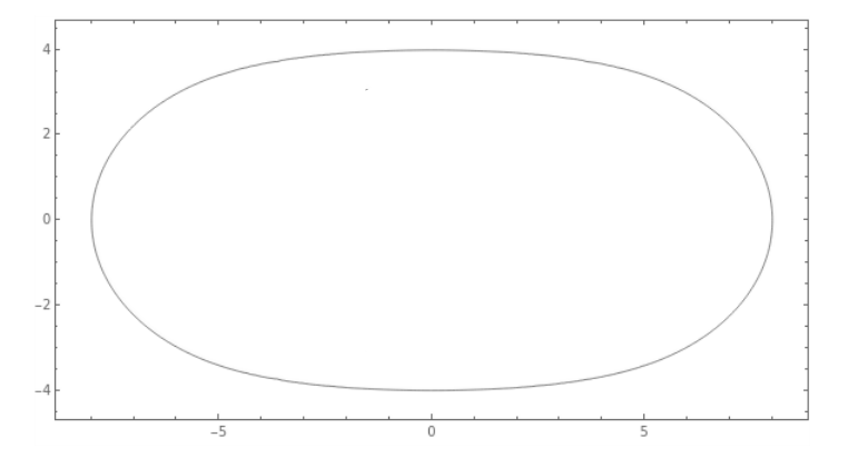
Example 2.9.

Let $a$ be the $2$-periodic sequence with period word $1\ 3$, let $b$ be the constant $0$ sequence and let $c$ be the $2$-periodic sequence with period word $4\ 8$. Then, by Proposition 2.8, if

$$S=\begin{pmatrix}8&\frac{1}{2}i&-\frac{7}{2}i&0\\[5.0pt] \frac{1}{2}i&1&0&-\frac{7}{2}i\\[5.0pt] -\frac{7}{2}i&0&-1&\frac{1}{2}i\\[5.0pt] 0&-\frac{7}{2}i&\frac{1}{2}i&-8\end{pmatrix},$$

then $\overline{W(T(a,b,c))}=W(S)$. The boundary of the numerical range of $S$ is shown in Figure 1. The Kippenhahn polynomial of $S$ equals

$$P(t,x,y)=t^{4}-65t^{2}x^{2}-25t^{2}y^{2}+64x^{4}+192x^{2}y^{2}+144y^{4}.$$

The quartic curve $P(t,x,y)=0$ in the complex projective plane has a pair of ordinary singular points of multiplicity $2$ at $(t,x,y)=(0,1,\pm i\sqrt{2/3})$ and there is no other singular point. So the algebraic curve theory tell us that the homogeneous polynomial $P(t,x,y)$ is irreducible in the polynomial ring.

Figure 1. Boundary of the numerical range of $S$

Hence, using for example Proposition 2.3 in [8], there cannot be a matrix $R$ of size $m\times m$, with $1\leq m<4$ with $W(R)=W(S)$. Incidentally, this shows that the size of the matrix $A$ in Theorem 2.7 is optimal.

Example 2.10.

Let $a$ and $c$ be real $2$-periodic sequences with period words $a_{0}a_{1}$ and $c_{0}c_{1}$ respectively, and let $b$ be the constant sequence $0$. If $a_{0}=c_{1}$, then $\gamma_{1}=0$ and then, by Proposition 2.8, $\overline{W(T(a,b,c))}=W(S)$, where

$$S=\begin{pmatrix}\alpha_{0}+\alpha_{1}&-\gamma_{0}&0&0\\ -\gamma_{0}&-\alpha_{0}+\alpha_{1}&0&0\\ 0&0&\alpha_{0}-\alpha_{1}&-\gamma_{0}\\ 0&0&-\gamma_{0}&-\alpha_{0}-\alpha_{1}\end{pmatrix}.$$

But this implies that

$$\overline{W(T(a,b,c))}=\mathrm{conv}\left(W(A+\alpha_{1}I)\cup W(A-\alpha_{1}I)\right),$$

where

$$A=\begin{pmatrix}\alpha_{0}&-\gamma_{0}\\ -\gamma_{0}&-\alpha_{0}\end{pmatrix}.$$

That is, $\overline{W(T(a,b,c))}$ is the convex hull of two ellipses (possibly degenerate), each one a translation of a single elllipse (possibly degenarate) centered at the origin.

Example 2.11.

Let $a$ be the $2$-periodic sequence with period word $1,-1$, let $b$ be the constant $0$ sequence and let $c$ be the constant $1$ sequence. Then, by Example 2.10, we have that $\overline{W(T(a,b,c))}=\mathrm{conv}\left(W(A+I)\cup W(A-I)\right)$, where

$$A=\begin{pmatrix}0&i\\[5.0pt] i&0\end{pmatrix}.$$

But it is easy to see that $W(A)$ is the closed line segment joining $-i$ and $i$. Hence, $\overline{W(T(a,b,c))}$ equals the convex hull of the closed line segment joining $-1-i$ and $-1+i$ and the closed line segment joining $1-i$ and $1+i$; i.e., the square with vertices $-1-i$, $-1+i$, $1-i$ and $1+i$, recovering (most of) Theorem 9 in [5].

Example 2.12.

Let $a$ and $c$ be real $2$-periodic sequences with period words $a_{0}a_{1}$ and $c_{0}c_{1}$ respectively, and let $b$ be the constant sequence $0$. If $c_{0}=a_{1}$, then $\gamma_{0}=0$ and then, by Proposition 2.8, $\overline{W(T(a,b,c))}=W(S)$, where

$$S=\begin{pmatrix}\alpha_{0}+\alpha_{1}&0&-\gamma_{1}&0\\ 0&-\alpha_{0}+\alpha_{1}&0&-\gamma_{1}\\ -\gamma_{1}&0&\alpha_{0}-\alpha_{1}&0\\ 0&-\gamma_{1}&0&-\alpha_{0}-\alpha_{1}\end{pmatrix}.$$

But if

$$U=\begin{pmatrix}1&0&0&0\\ 0&0&1&0\\ 0&1&0&0\\ 0&0&0&1\end{pmatrix},$$

then

$$U^{*}SU=\begin{pmatrix}\alpha_{0}+\alpha_{1}&-\gamma_{1}&0&0\\ -\gamma_{1}&\alpha_{0}-\alpha_{1}&0&0\\ 0&0&-\alpha_{0}+\alpha_{1}&-\gamma_{1}\\ 0&0&-\gamma_{1}&-\alpha_{0}-\alpha_{1}\end{pmatrix}.$$

But this implies that

$$\overline{W(T(a,b,c))}=\mathrm{conv}\left(W(A+\alpha_{0}I)\cup W(A-\alpha_{0}I)\right),$$

where

$$A=\begin{pmatrix}\alpha_{1}&-\gamma_{1}\\ -\gamma_{1}&-\alpha_{1}\end{pmatrix}.$$

That is, $\overline{W(T(a,b,c))}$ is the convex hull of two ellipses (possibly degenerate), each one a translation of a single elllipse (possibly degenarate) centered at the origin.

Example 2.13.

Let $a$ be the $2$-periodic sequence with period word $01$, let $b$ be the constant $0$ sequence and let $c$ be the constant $1$ sequence. Then, by Example 2.12, we have that $\overline{W(T(a,b,c))}=\mathrm{conv}\left(W(A+I)\cup W(A-I)\right)$, where

$$A=\begin{pmatrix}\frac{1}{2}&-\frac{1}{2}i\\[5.0pt] -\frac{1}{2}i&-\frac{1}{2}\end{pmatrix}.$$

But, if

$$U=\begin{pmatrix}\frac{1}{\sqrt{2}}&\frac{1}{\sqrt{2}}\\[10.0pt] -\frac{1}{\sqrt{2}}i&\frac{1}{\sqrt{2}}i\end{pmatrix},$$

then $U$ is unitary and $U^{*}AU$ equals

$$\begin{pmatrix}0&1\\ 0&0\end{pmatrix}.$$

Therefore, $\overline{W(T(a,b,c))}=\mathrm{conv}\left(W(B+I)\cup W(B-I)\right)$, recovering the result in [14, Theorem 3.6].

In the paper [15] we explore some sufficient conditions under which the matrix $A$ can be explicitly found, namely if $b=0$ and there is some symmetry in the periodic sequences $a$ and $c$, then the polynomial $P$ can be factored as the product of the Kippenhahn polynomials of two computable matrices, which generalizes the previous four examples.

References

- [1] N. Bebiano, J. da Providência, and A. Nata. The numerical range of banded periodic Toeplitz operators. J. Math. Anal. Appl., 398:189–197, 2013.
- [2] S.N. Chandler-Wilde, R. Chonchaiya, and M. Lindner. Eigenvalue problem meets Sierpinski triangle: computing the spectrum of a non-self-adjoint random operator. Oper. Matrices, 5:633–648, 2011.
- [3] S. N. Chandler-Wilde, R. Chonchaiya, and M. Lindner. On the spectra and pseudospectra of a class of non-self-adjoint random matrices and operators. Oper. Matrices, 7:739–775, 2013.
- [4] S. N. Chandler-Wilde and E. B. Davies. Spectrum of a Feinberg-Zee random hopping matrix. J. Spectr. Theory, 2:147–179, 2012.
- [5] M. T. Chien and H. Nakazato. The numerical range of a tridiagonal operator. J. Math. Anal. Appl. 373:297-304, 2011.
- [6] R.T. Chien and I.M. Spitkovsky. On the numerical ranges of some tridiagonal matrices. Linear Algebra Appl., 470:228–240, 2015.
- [7] J. Feinberg and A. Zee. Spectral curves of non-hermitean Hamiltonians. Nuclear Phys. B, 552:599–623, 1999.
- [8] H. L. Gau and P. Y. Wu. Companion matrices: reducibility, numerical ranges and similarity to contractions. Linear Algebra Appl. 383:127–142, 2004.
- [9] R. Hagger. The eigenvalues of tridiagonal sign matrices are dense in the spectra of periodic tridiagonal sign operators. J. Funct. Anal., 269:1563–1570, 2015.
- [10] R. Hagger. On the spectrum and numerical range of tridiagonal random operators. J. Spectr. Theory, 6:215266, 2016.
- [11] J. W. Helton and I. M. Spitkovsky. The possible shapes of numerical ranges. Operators and Matrices, 6:607-611, 2012.
- [12] J. W. Helton and V. Vinnikov. Linear matrix inequality representations of sets. Communications on Pure and Applied Mathematics,60: 654-674, 2007.
- [13] C. Hernández-Becerra and B. A. Itzá-Ortiz. A class of tridiagonal operators associated to some subshifts. Open Math., 14:2391–5455, 2016.
- [14] B. A. Itzá-Ortiz and R. A. Martínez-Avendaño. The numerical range of a class of periodic tridiagonal operators. Linear Multilinear Algebra. 69:786–806, 2021.
- [15] B. A. Itzá-Ortíz, R. A. Martínez-Avendaño and H. Nakazato. The numerical range of some tridiagonal operators is the convex hull of the numerical ranges of two finite matrices. Preprint arXiv:2103.01866 [math.FA].
- [16] T. Kato. Perturbation theory for linear operators. Die Grundlehren der mathematischen Wissenschaften, Band 132. Springer-Verlag New York, Inc., New York, 1966.
- [17] R. Kippenhahn, Über den wertevorrat einer Matrix. Math. Nachr., 6:193-228, 1951.
- [18] R. Kippenhahn. On the numerical range of a matrix. Translated from the German by Paul F. Zachlin and Michiel E. Hochstenbach. Linear Multilinear Algebra 56:185-225, 2008.
- [19] D. Plaumann, B. Sturmfels and C. Vinzant, Computing linear matrix representations of Helton-Vinnikov curves, in Mathematical methods in systems, optimization, and control, Oper. Theory Adv. Appl. 222, 259–277, Birkhäuser/Springer Basel AG, Basel, 2012.
- [20] D. Plaumann and C. Vinzant. Determinantal representations of hyperbolic plane curves: An elementary approach, J. Symbolic Comput., 57:48–60, 2013.