Crossover from itinerant to localized states in the thermoelectric oxide [Ca₂CoO₃]_0.62[CoO₂]

Abstract

The layered cobaltite [Ca₂CoO₃]_0.62[CoO₂], often expressed as the approximate formula Ca₃Co₄O₉, is a promising candidate for efficient oxide thermoelectrics but an origin of its unusual thermoelectric transport is still in debate. Here we investigate in-plane anisotropy of the transport properties in a broad temperature range to examine the detailed conduction mechanism. The in-plane anisotropy between $a$ and $b$ axes is clearly observed both in the resistivity and the thermopower, which is qualitatively understood with a simple band structure of the triangular lattice of Co ions derived from the angle-resolved photoemission spectroscopy experiments. On the other hand, at high temperatures, the anisotropy becomes smaller and the resistivity shows a temperature-independent behavior, both of which indicate a hopping conduction of localized carriers. Thus the present observations reveal a crossover from low-temperature itinerant to high-temperature localized states, signifying both characters for the enhanced thermopower.

I Introduction

The layered cobaltites provide fascinating platform for exploring functional properties of oxides both in fundamental and applicational viewpoints [1]. Since the discovery of large thermopower in the metallic Na_xCoO₂ [2], this class of materials has been recognized as potential oxide thermoelectrics that possesses a high-temperature stability in air [3, 4, 5]. The crystal structure of this family is composed of two subsystems of an insulating layer and CdI₂-type CoO₂ conduction layer alternately stacked along the $c$ axis. As for the origin of the large thermopower coexisting with the metallic conductivity, Koshibae et al. have suggested a localized model in which a hopping conduction of correlated $d$ electrons with spin and orbital degeneracies involves large entropy flow [6]. This picture is supported by magnetic field dependence of the thermopower [7] and is also discussed in semiconducting cobalt oxides [8]. On the other hand, Kuroki et al. have proposed an itinerant model based on “pudding-mold” band structure, in which the difference in velocities of electrons and holes is crucial [9]. Indeed, such a peculiar band shape is observed by angle-resolved photoemission spectroscopy (ARPES) experiments [10, 11, 12, 13, 14] and a large value of thermopower is calculated accordingly [15, 16], remaining the detailed conduction mechanism in this system controversial.

The misfit oxide [Ca₂CoO₃]_0.62[CoO₂] [17, 18, 19] is a suitable compound to shed light on above fundamental issue, because it straddles a border between localized and itinerant states of Co $3d$ electrons, from which interesting emergent phenomena appear in correlated electron systems [20]. As shown in Figs. 1(a) and 1(b), this material has a rocksalt-type Ca₂CoO₃ block as an insulating layer and its $b$-axis lattice parameter $b_{2}$ is different from that of CoO₂ layer $b_{1}$, leading to a misfit structure with incommensurate ratio of $b_{1}/b_{2}\simeq 0.62$ while this system is often referred as the approximate formula Ca₃Co₄O₉. The metallic transport properties, along with a spin-density-wave (SDW) formation at $T_{\rm SDW}\simeq 30$ K [22, 23, 24], indicate an itinerant nature, although the magnetic structure revealed by recent neutron experiments is quite unconventional [25]. On the other hand, compared with that of Na_xCoO₂, this compound has moderately high resistivity [26], which is close to the Ioffe-Regel limit [18]. Negative magnetothermopower is also found in [Ca₂CoO₃]_0.62[CoO₂] [27]. In addition, large thermopower of $Q\simeq 130$ $\mu$V/K near room temperature is well explained in the extended Heikes formula based on the localized hopping picture of correlated electrons [28], which prevails not only in the conduction layer but also the rocksalt one as suggested by recent spectroscopic studies [29]. These experimental facts imply a complicated coexistence of itinerant and localized nature in this compound.

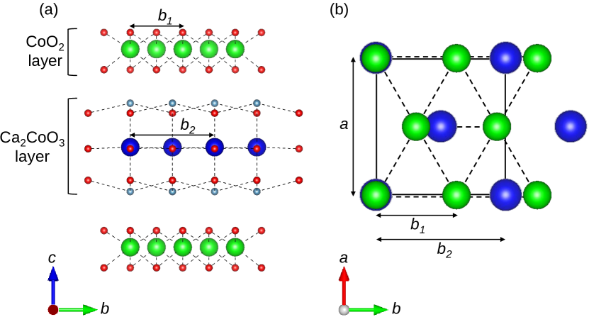
Figure 1: Schematic view of the crystal structure of layered [Ca₂CoO₃]_0.62[CoO₂] projected from (a) $a$ axis and (b) $c$ axis drawn by VESTA [21]. While the $a$-axis lattice parameter $a$ is common, the $b$-axis lattice parameter of the rocksalt layer $b_{2}$ is different from that of CoO₂ layer $b_{1}$, resulting in a misfit structure with incommensurate ratio of $b_{1}/b_{2}\simeq 0.62$. The Co ions in CoO₂ (green) and rocksalt (blue) layers are shown in different colors for clarity.

In this study, we argue the itinerancy and localization of conduction electrons in [Ca₂CoO₃]_0.62[CoO₂] by means of in-plane transport anisotropy measurements between $a$- and $b$-axis directions. This is less investigated so far compared to the strong anisotropy between in-plane and out-of-plane directions [18, 30] but is essential for thorough understanding of the underlying conduction mechanism. We find a considerable temperature dependence of the in-plane anisotropy both in resistivity and thermopower. Below room temperature, the in-plane anisotropy is relatively large and qualitatively explained by the anisotropy of the electronic velocities near the Fermi energy estimated from the results of ARPES experiments [31]. This is also consistent with the results of recent band calculation [32], indicating the itinerant nature in this system. Near $T_{\rm SDW}\simeq 30$ K, the in-plane anisotropy drastically varies possibly due to a reconstruction of the Fermi surface. Above room temperature, in contrast, we find that the in-plane anisotropy is close to unity as temperature increases, which is captured as a localized picture. The present results unveil the temperature-induced crossover from itinerant to localized states in [Ca₂CoO₃]_0.62[CoO₂].

II Experiments

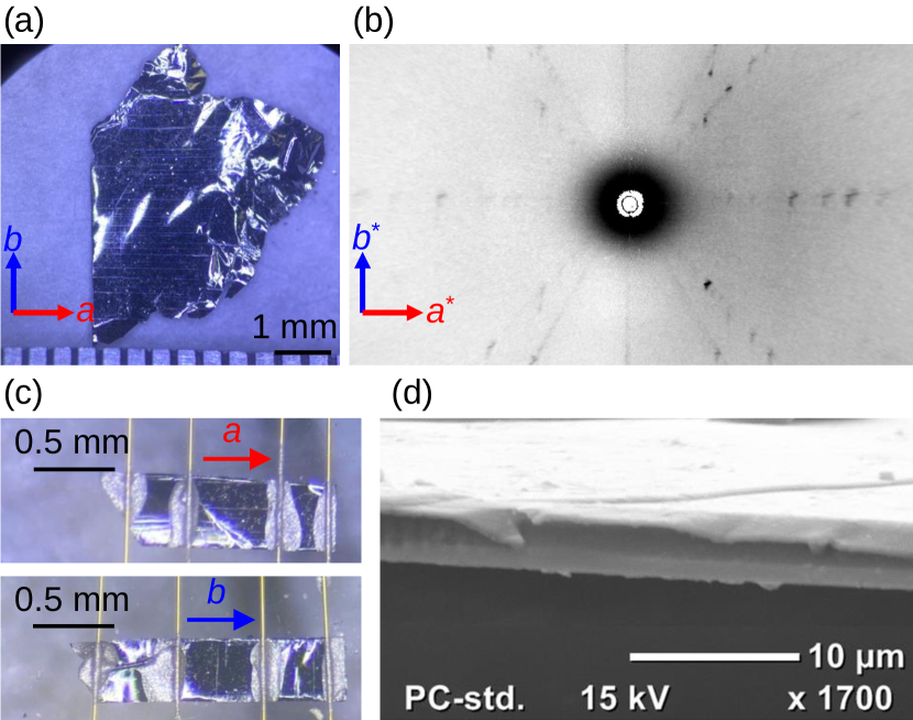
Figure 2: (a) Photograph of a single crystal of [Ca₂CoO₃]_0.62[CoO₂] and (b) Laue pattern. (c) Photographs of samples for the resistivity measurements. Two samples with the rectangular shape of $\sim 1\times 0.3$ mm² were obtained by cutting one single crystal. (d) SEM image of [Ca₂CoO₃]_0.62[CoO₂] for the sample thickness measurement.

Single crystals of [Ca₂CoO₃]_0.62[CoO₂] were grown by a flux method [33]. Powders of CaCO₃ (99.9%) and Co₃O₄ (99.9%) were mixed in a stoichiometric ratio and calcined two times in air at 1173 K for 20 h with intermediate grindings. Then KCl (99.999%) and K₂CO₃ (99.999%) powders mixed with a molar ratio of $1:4$ was added with the calcined powder as a flux. The concentration of [Ca₂CoO₃]_0.62[CoO₂] was set to be 1.5% in molar ratio. The mixture was put in an alumina crucible and heated up to 1123 K in air with a heating rate of 200 K/h. After keeping 1123 K for 1 h, it was slowly cooled down with a rate of 1 K/h, and at 1023 K, the power of the furnace was switched off. As-grown samples were rinsed in distilled water to remove the flux and then annealed in air at 573 K for 3 h.

The typical dimension of obtained single crystals is $\simeq 4\times 4\times 0.01$ mm³ as shown in Fig. 2(a). The crystal orientation was determined by the Laue method. Although the spot intensity is weak in such thin samples, three-fold symmetry from CoO₂ layer and four-fold symmetry from the rocksalt layer are resolved in the Laue pattern shown in Fig. 2(b). To discuss the anisotropy precisely, we cut one single crystal into two samples with the same rectangular shape of $\simeq 1\times 0.3$ mm² for the transport measurements along the $a$ and $b$ axes as shown in Fig. 2(c). This method enables us to compare the transport properties of the samples with the same oxygen contents. Note that the resistivity anisotropy was also checked by utilizing the Montgomery method near room temperature [34], although it may produce a fairly large systematic error bar [35]. The sample thickness of $\simeq 5$ $\mu$m was determined by the scanning electron microscopy (SEM) as shown in Fig. 2(d). The resistivity and the thermopower were simultaneously measured by using a conventional four-probe method and a steady-state method, respectively. The thermoelectric voltage from the wire leads was carefully subtracted. We used a Gifford-McMahon refrigerator below room temperature and an electrical furnace for high-temperature measurement.

III Results and discussion

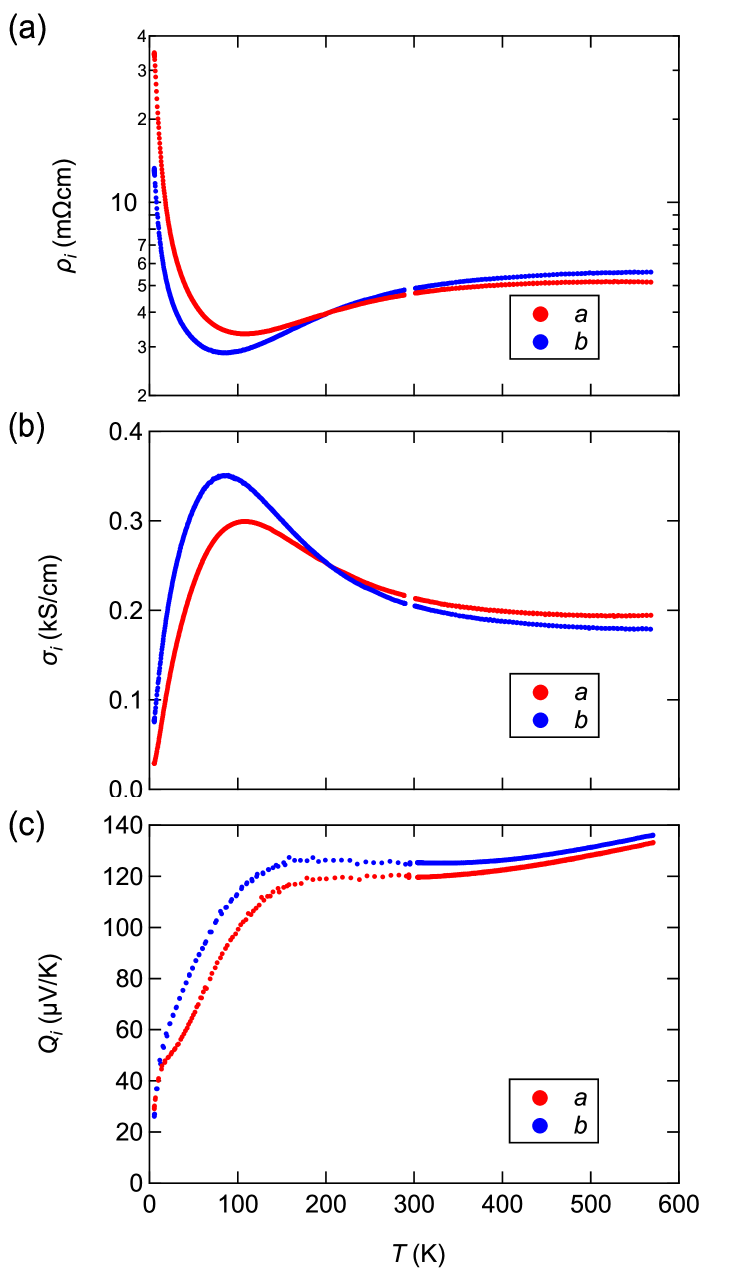
Figure 3: Temperature variations of (a) resistivity $\rho_{i}$ ($i=a,b$), (b) conductivity $\sigma_{i}=\rho_{i}^{-1}$, and (c) thermopower $Q_{i}$ measured along the $a$- (red) and $b$-axis (blue) directions in [Ca₂CoO₃]_0.62[CoO₂].

III.1 Temperature variations of resistivity and thermopower

Figures 3 summarize the temperature variations of the in-plane transport properties in [Ca₂CoO₃]_0.62[CoO₂]. Hereafter we use an abbreviated form like $\rho_{a}(=\rho_{aa})$ for the resistivity measured along the $a$-axis direction. Overall behaviors are well reproduced compared with the earlier reports in which the transport coefficients are measured with no distinction among the in-plane directions [18]. In addition, the thermopower measured along the $b$ axis $Q_{b}$ is larger than that along the $a$ axis $Q_{a}$, consistent with recent theoretical calculation [32]. At low temperature below $\sim 100$ K, the resistivity shows an insulating behavior while the thermopower seems to be metallic, which are discussed in terms of carrier localization [36], pseudogap opening [37], or quantum criticality [38]. Near room temperature, the thermopower shows a temperature-independent behavior with a relatively large value of $Q\simeq 130$ $\mu$V/K, quantitatively explained by the extended Heikes formula of

$$Q=-\frac{k_{B}}{e}\ln\left(\frac{g_{3}}{g_{4}}\frac{y}{1-y}\right),$$ (1)

where $k_{B}$ is the Boltzmann coefficient, $e$ the elementary charge, $g_{3}$ and $g_{4}$ the spin and orbital degeneracies of Co³⁺ and Co⁴⁺ ions, respectively, and $y$ the Co⁴⁺ (hole) concentration [6]. Enhancement of the thermopower above room temperature may be possibly attributed to a small spin-state change near $T\simeq 380$ K [39], above which the degeneracy ratio $g_{3}/g_{4}$ may vary with temperature. At this temperature, a small anomaly has been observed in several quantities such as the resistivity, magnetic susceptibility, heat capacity, and lattice constants [18, 22, 39]. On the other hand, the magnitude of the resistive anomaly may be sample-dependent [40] and is not resolved in the present samples. Although the present measurements are limited below 600 K, the increase of thermopower may continue up to 1000 K according to high-temperature transport experiments in this compound [41].

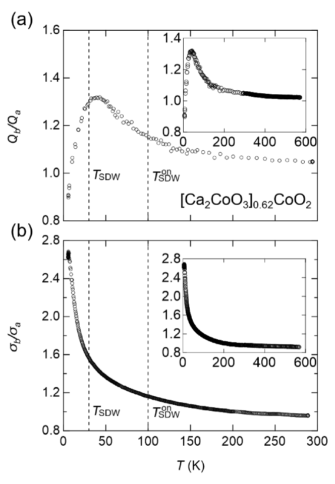
Figure 4: Temperature variations of the transport anisotropy in (a) thermopower $Q_{b}/Q_{a}$ and (b) electrical conductivity $\sigma_{b}/\sigma_{a}$ below room temperature. The SDW transition temperature $T_{\rm SDW}\simeq 30$ K and its onset $T_{\rm SDW}^{\rm ON}\simeq 100$ K are indicated by the dashed lines. The insets depict these anisotropies in the whole temperature range measured in the present study.

III.2 Localized state at high temperatures

We first discuss high-temperature transport. The inset of Fig. 4(a) shows the temperature dependence of the anisotropy of thermopower $Q_{b}/Q_{a}$. The anisotropy $Q_{b}/Q_{a}$ decreases with increasing temperature and becomes close to unity near 600 K. This behavior is well consistent with the localized model, because the thermopower at high temperatures can be expressed by using chemical potential $\mu$ as

$$Q=-\frac{\mu}{eT},$$ (2)

which leads to the Heikes formula of Eq. (1) [6], and the chemical potential in the numerator is a thermodynamic quantity, which does not give the anisotropic property. Note that other parameters to produce the anisotropy such as velocity and relaxation time are cancelled out in Eq. (2). Therefore, the thermopower anisotropy, which should be unity within the Heikes formula, is an indicator for localized electronic state.

Moreover, as shown in Fig. 3(a), the resistivity becomes less temperature-dependent in both directions at high temperatures. Such a behavior has also been observed in high-temperature transport study while the in-plane orientation is undetermined [41], and is described as the hopping conduction at the Ioffe-Regel limit [42, 43, 44], at which the Fermi wavelength $\lambda_{F}(=2\pi/k_{F})$ ($k_{F}$ being Fermi wavenumber) is comparable to the mean free path $l$ of conduction electrons. Indeed, the dimensionless value of $k_{F}l$ estimated from

$$k_{F}l=\frac{2\pi\hbar c_{0}}{e^{2}\rho},$$ (3)

where $\hbar$ is the reduced Planck constant and $c_{0}$ is the $c$-axis length [37], is calculated as $k_{F}l\sim 0.54$ for the $a$- and $0.50$ for the $b$-axis directions. Although there is an unavoidable error bar mainly due to the sample thickness, these values are close to unity, indicating the hopping conduction. Thus, these transport coefficients indicate the localized nature at high temperatures.

III.3 Itinerant state at low temperatures

We then focus on low-temperature transport anisotropy below room temperature. The main panels of Figs. 4(a) and 4(b) show the temperature variations of the anisotropies of thermopower $Q_{b}/Q_{a}$ and electrical conductivity $\sigma_{b}/\sigma_{a}$ below room temperature, respectively. In temperature range of 40 K $\lesssim T\lesssim$ 300 K, both $Q_{b}/Q_{a}$ and $\sigma_{b}/\sigma_{a}$ increase with lowering temperature. Note that similar behaviors in thermopower and conductivity are also observed in the related layered cobalitite (Bi,Pb)₂Sr₂Co₂O_y [45], implying a universal anisotropic property in the CoO₂-based materials as is discussed below.

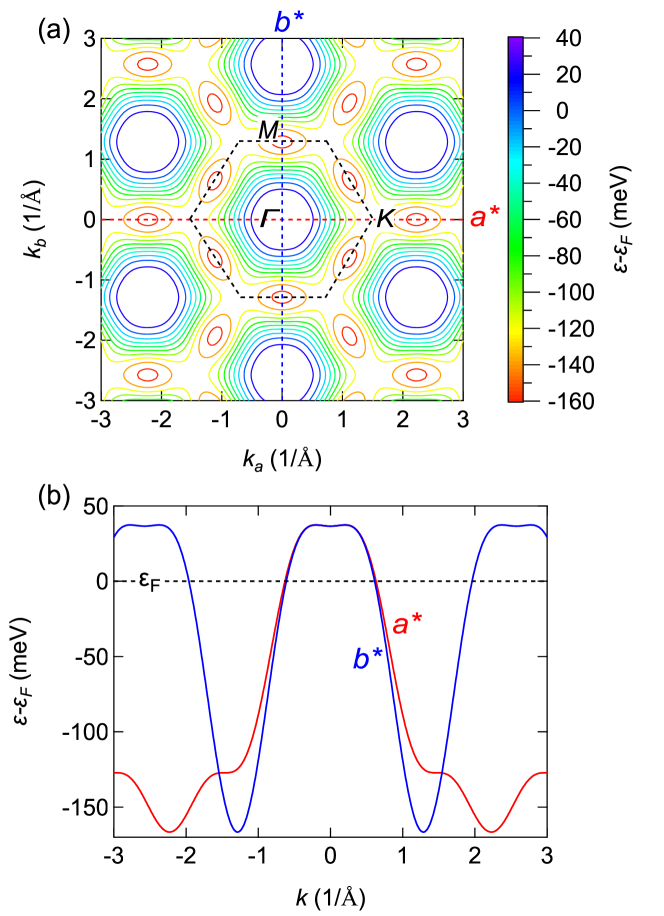
Figure 5: (a) Constant-energy surfaces near the Fermi energy calculated by using the tight-binding model [Eq. (4)]. (b) Dispersion relations along $\Gamma\to{\rm K}$ ($a^{*}$ direction, red) and $\Gamma\to{\rm M}$ ($b^{*}$ direction, blue).

To clarify the origin of the anisotropic transport at low temperatures, we discuss the electronic band structure measured by ARPES at $T=40$ K [31]. Note that the band structure is also proposed theoretically but there is a difficulty originating from the misfit structure of this system, in which an approximate formula is required for calculations [32, 46, 47, 48, 49]. In fact, the calculated thermopower strongly depends on the calculation methods [32, 49]. Thus, the present results may offer an experimental clue for the challenging issue to theoretically obtain the transport properties precisely in correlated electron systems with an incommensurate structure like this material. Now the band structure experimentally obtained in [Ca₂CoO₃]_0.62[CoO₂] is well fitted by a tight-binding dispersion relation for the hexagonal lattice with primitive vectors $\vec{a_{h}}$ and $\vec{b_{h}}$ as [50]

$$\varepsilon({\bm{k}}) =\varepsilon_{0}-2t\left\{\cos(k_{a}a_{h})+2\cos\left(\frac{\sqrt{3}}{2}k_{b}a_{h}\right)\cos\left(\frac{k_{a}a_{h}}{2}\right)\right\}$$

$$-2t^{\prime}\left\{\cos(2k_{a}a_{h})+2\cos\left(\sqrt{3}k_{b}a_{h}\right)\cos\left(k_{a}a_{h}\right)\right\},$$ (4)

where $\varepsilon_{0}=-72.6$ meV is a constant and $a_{h}=2.82$ Å the lattice constant. In this model, the conducting CoO₂ layer is considered only, and modeled as a hexagonal lattice. $t=-25.4$ meV and $t^{\prime}=7.2$ meV denote the transfer integrals between atomic orbitals connected with $\vec{a_{h}}$ and those with $2\vec{a_{h}}$. As is discussed in Ref. 31, tight-binding fit with $t^{\prime\prime}$, which is transfer integral along $\vec{a_{h}}+\vec{b_{h}}$ direction, leads to wrong result probably due to a one-dimensional $\sigma$-bond formation along $\vec{a_{h}}$ direction. Figure 5(a) shows the calculated contour plot for the constant-energy surfaces, in which a Fermi surface with a hexagonal shape is confirmed as seen in ARPES experiments [31]. Note that $k_{a}$ and $k_{b}$ directions correspond to $\sim a$ and $b$ directions in real space, respectively [51].

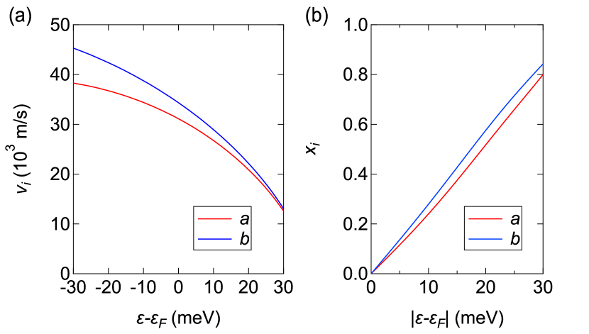
Figure 6: (a) Electronic velocity $v_{i}=1/\hbar(\partial\varepsilon/\partial k_{i})$ as a function of energy measured from the Fermi energy for $a$ (red) and $b$ (blue) directions. The velocity $v_{a}$ ($v_{b}$) is calculated for $k_{b}=0$ ($k_{a}=0$). (b) A velocity ratio $x_{i}\equiv(v^{2}_{i,h}-v^{2}_{i,e})/(v^{2}_{i,h}+v^{2}_{i,e})$ for $a$ (red) and $b$ (blue) directions as a function of the energy measured from $\varepsilon_{F}$ in magnitude.

Figure 5(b) shows the dispersion relations along the $\Gamma\to{\rm K}$ and $\Gamma\to{\rm M}$ directions. The flat region in the top of these dispersions indicates a pudding mold energy band, in which the thermopower is approximately determined by the difference in the velocities of electrons and holes as [9]

$$Q_{i}=\frac{k_{B}}{e}\frac{\sum(v^{2}_{i,h}-v^{2}_{i,e})}{\sum(v^{2}_{i,h}+v^{2}_{i,e})},$$ (5)

where $v_{i,e}$ and $v_{i,h}$ are the velocities of electrons and hole for the $i$ direction ($i=a,b$), respectively. Figure 6(a) presents the carrier velocity calculated as $v_{a}=1/\hbar(\partial\varepsilon/\partial k_{a})|_{k_{b}=0}$ and $v_{b}=1/\hbar(\partial\varepsilon/\partial k_{b})|_{k_{a}=0}$ as a function of energy near the Fermi energy. Although the summation in Eq. (5) is taken over all the ${\bm{k}}$ states within the thermal energy $k_{B}T$, for simplicity we only consider these $v_{a}$ and $v_{b}$, which largely contribute to the transport coefficients for each direction. In this approximation, one obtains $v_{i,e}=v_{i}(\varepsilon>\varepsilon_{F})$ and $v_{i,h}=v_{i}(\varepsilon<\varepsilon_{F})$. Figure 6(b) depicts a velocity ratio $x_{i}\equiv(v^{2}_{i,h}-v^{2}_{i,e})/(v^{2}_{i,h}+v^{2}_{i,e})$ for each direction as a function of the energy from the Fermi energy in magnitude. In the present energy range, which is comparable to the thermal energy $k_{B}T$, $x_{b}>x_{a}$ holds, leading to $Q_{b}>Q_{a}$. This is consistent with the present result shown in Fig. 3(c), indicating a validity of itinerant picture based on the observed Fermi surface.

We mention the anisotropy in the SDW phase below 30 K. This material shows the SDW transition at $T_{\rm SDW}\simeq 30$ K and its onset temperature is $T_{\rm SDW}^{\rm ON}\simeq 100$ K. As shown in Fig. 4(a), although no prominent feature is found at $T_{\rm SDW}^{\rm ON}$, we observed a cusp near $T_{\rm SDW}$ in the temperature dependence of the thermopower anisotropy. The cusp structure in the thermopower anisotropy indicates that the electronic structure is drastically varied at $T_{\rm SDW}$, as is seen in the significant change in thermopower anisotropy at the SDW transition in Fe-based superconductors [52]. On the other hand, the conductivity anisotropy $\sigma_{b}/\sigma_{a}$ is monotonically increased as temperature decreases and shows no anomaly at $T_{\rm SDW}$ as seen in Fig. 4(b). This result implies that, although the anisotropy of the velocities is crucial since $v_{b}>v_{a}$ leads to $\sigma_{b}>\sigma_{a}$ from $\sigma_{i}\sim\sum\left(v^{2}_{i,h}+v^{2}_{i,e}\right)\tau$, where $\tau$ is the relaxation time, the conductivity anisotropy may be governed by the relaxation time, which is cancelled out in the thermopower formula of Eq. (5).

IV Summary

To summarize, we have measured the anisotropies of the resistivity and the thermopower in the layered [Ca₂CoO₃]_0.62[CoO₂] and found the considerable temperature variations. In high-temperature range, the anisotropy in the thermopower becomes close to unity, indicating a localized picture. On the other hand, low-temperature anisotropies are qualitatively explained in the itinerant band picture based on the results from ARPES, and the change in the electronic structure associated with the SDW transition is probed as a cusp behavior of the thermopower anisotropy. These results show a crossover from low-temperature itinerant to high-temperature localized electronic states in this material.

- [1] F. Schipper, E. M. Erickson, C. Erk, J.-Y. Shin, F. F. Chesneau, and D. Aurbach, J. Electrochem. Soc. 164, A6220 (2017).
- [2] I. Terasaki, Y. Sasago, and K. Uchinokura, Phys. Rev. B 56, R12685 (1997).
- [3] G. J. Snyder and E. S. Toberer, Nat. Mater. 7, 105 (2008).
- [4] K. Koumoto, Y. Wang, R. Zhang, A. Kosuga, and R. Funahashi, Annu. Rev. Mater. Res. 40, 363 (2010).
- [5] S. Hébert, D. Berthebaud, R. Daou, Y. Bréard, D. Pelloquin, E. Guilmeau, F. Gascoin, O. Lebedev, and A. Maignan, J. Phys.: Condens. Matter 28, 013001 (2016).
- [6] W. Koshibae, K. Tsutsui, and S. Maekawa, Phys. Rev. B 62, 6869 (2000).
- [7] Y. Wang, N. S. Rogado, R. J. Cava, and N. P. Ong, Nature 423, 22 (2003).
- [8] H. Takahashi, S. Ishiwata, R. Okazaki, Y. Yasui, and I. Terasaki, Phys. Rev. B 98, 024405 (2018).
- [9] K. Kuroki and R. Arita, J. Phys. Soc. Jpn. 76, 083707 (2007).
- [10] H.-B. Yang, S.-C. Wang, A. K. P. Sekharan, H. Matsui, S. Souma, T. Sato, T. Takahashi, T. Takeuchi, J. C. Campuzano, R. Jin, B. C. Sales, D. Mandrus, Z. Wang, and H. Ding, Phys. Rev. Lett. 92, 246403 (2004).
- [11] H.-B. Yang, Z.-H. Pan, A. K. P. Sekharan, T. Sato, S. Souma, T. Takahashi, R. Jin, B. C. Sales, D. Mandrus, A. V. Fedorov, Z. Wang, and H. Ding, Phys. Rev. Lett. 95, 146401 (2005).
- [12] D. Qian, L. Wray, D. Hsieh, D. Wu, J. L. Luo, N. L. Wang, A. Kuprin, A. Fedorov, R. J. Cava, L. Viciu, and M. Z. Hasan, Phys. Rev. Lett. 96, 046407 (2006).
- [13] J. Geck, S. V. Borisenko, H. Berger, H. Eschrig, J. Fink, M. Knupfer, K. Koepernik, A. Koitzsch, A. A. Kordyuk, V. B. Zabolotnyy, and B. Büchner, Phys. Rev. Lett. 99, 046403 (2007).
- [14] T. Arakane, T. Sato, T. Takahashi, T. Fujii, and A. Asamitsu, New J. Phys. 13, 043021 (2011).
- [15] N. Hamada, T. Imai, and H. Funashima, J. Phys.: Condens. Matter 19, 365221 (2007).
- [16] S.-D. Chen, Y. He, A. Zong, Y. Zhang, M. Hashimoto, B.-B. Zhang, S.-H. Yao, Y.-B. Chen, J. Zhou, Y.-F. Chen, S.-K. Mo, Z. Hussain, D. Lu, and Z.-X. Shen, Phys. Rev. B 96, 081109(R) (2017).
- [17] R. Funahashi, I. Matsubara, H. Ikuta, T. Takeuchi, U. Mizutani, and S. Sodeoka, J. Appl. Phys. 39, L1127 (2000).
- [18] A. C. Masset, C. Michel, A. Maignan, M. Hervieu, O. Toulemonde, F. Studer, B. Raveau, and J. Hejtmanek, Phys. Rev. B 62, 166 (2000).
- [19] Y. Miyazaki, M. Onoda, T. Oku, M. Kikuchi, Y. Ishii, Y. Ono, Y. Morii, and T. Kajitani, J. Phys. Soc. Jpn. 71, 491 (2002).
- [20] E. Dagotto, Science 309, 257 (2005).
- [21] K. Momma and F. Izumi, J. Appl. Crystallogr. 44, 1272 (2011).
- [22] J. Sugiyama, H. Itahara, T. Tani, J. H. Brewer, and E. J. Ansaldo, Phys. Rev. B 66, 134413 (2002).
- [23] J. Sugiyama, J. H. Brewer, E. J. Ansaldo, H. Itahara, K. Dohmae, Y. Seno, C. Xia, and T. Tani, Phys. Rev. B 68, 134423 (2003).
- [24] N. Murashige, F. Takei, K. Saito, and R. Okazaki, Phys. Rev. B 96, 035126 (2017).
- [25] A. Ahad, K. Gautam, K. Dey, S. S. Majid, F. Rahman, S. K. Sharma, J. A. H. Coaquira, Ivan da Silva, E. Welter, and D. K. Shukla, Phys. Rev. B 102, 094428 (2020).
- [26] M. Mikami, K. Chong, Y. Miyazaki, T. Kajitani, T. Inoue, S. Sodeoka and R. Funahashi, J. Appl. Phys. 45, 4131 (2006).
- [27] P. Limelette, S. Hébert, V. Hardy, R. Frésard, Ch. Simon, and A. Maignan, Phys. Rev. Lett. 97, 046601 (2006).
- [28] R. F. Klie, Q. Qiao, T. Paulauskas, A. Gulec, A. Rebola, S. Öğüt, M. P. Prange, J. C. Idrobo, S. T. Pantelides, S. Kolesnik, B. Dabrowski, M. Ozdemir, C. Boyraz, D. Mazumdar, and A. Gupta, Phys. Rev. Lett. 108, 196601 (2012).
- [29] A. Ahad, K. Gautam, S. S. Majid, S. Francoual, F. Rahman, F. M. F. De Groot, and D. K. Shukla, Phys. Rev. B 101, 220202(R) (2020).
- [30] G. D. Tang, H. H. Guo, T. Yang, D. W. Zhang, X. N. Xu, L. Y. Wang, Z. H. Wang, H. H. Wen, Z. D. Zhang, and Y. W. Du, Appl. Phys. Lett. 98, 202109 (2011).
- [31] T. Takeuchi, T. Kondo, T. Kitao, K. Soda, M. Shikano, R. Funahashi, M. Mikami, and U. Mizutani, J. Electron Spectrosc. Relat. Phenom. 144-147, 849 (2005).
- [32] S. Lemal, J. Varignon, D. I. Bilc, and P. Ghosez, Phys. Rev. B 95, 075205 (2017).
- [33] Y. Ikeda, K. Saito, and R. Okazaki, J. Appl. Phys. 119, 225105 (2016).
- [34] C. A. M. dos Santos, A. de Campos, M. S. da Luz, B. D. White, J. J. Neumeier, B. S. de Lima, and C. Y. Shigue, J. Appl. Phys. 110, 083703 (2011).
- [35] M. A. Tanatar, N. Ni, G. D. Samolyuk, S. L. Budko, P. C. Canfield, and R. Prozorov, Phys. Rev. B 79, 134528 (2009).
- [36] A. Bhaskar, Z.-R. Lin, and C.-J. Liu, J. Mater. Sci. 49, 1359 (2014).
- [37] Y.-C. Hsieh, R. Okazaki, H. Taniguchi, and I. Terasaki, J. Phys. Soc. Jpn. 83, 054710 (2014).
- [38] P. Limelette, W. Saulquin, H. Muguerra, and D. Grebille, Phys. Rev. B 81, 115113 (2010).
- [39] T. Wu, T. A. Tyson, H. Chen, J. Bai, H. Wang and C. Jaye, J. Phys.: Condens. Matter 24, 455602 (2012).
- [40] J. Hejtmánek, Z. Jirák, and J. Šebek, Phys. Rev. B 92, 125106 (2015).
- [41] M. Shikano and R. Funahashi, Appl. Phys. Lett. 82, 1851 (2003).
- [42] A. F. Ioffe and A. R. Regel, Prog. Semicond. 4, 237 (1960).
- [43] M. Gurvitch, Phys. Rev. B 24, 7404 (1981).
- [44] N. E. Hussey, K. Takenaka, and H. Takagi, Philos Mag 84, 27 (2004).
- [45] T. Fujii, I. Terasaki, T. Watanabe and A. Matsuda, J. Appl. Phys. 45, 4131 (2006).
- [46] R. Asahi, J. Sugiyama, and T. Tani, Phys. Rev. B 66, 155103 (2002).
- [47] J. Soret and M.-B. Lepetit, Phys. Rev. B 85, 165145 (2012).
- [48] A. Rébola, R. Klie, P. Zapol, and S. Öğüt, Phys. Rev. B 85, 155132 (2012).
- [49] B. Amin, U. Eckern, and U. Schwingenschlögl, Appl. Phys. Lett. 110, 233505 (2017).
- [50] B. J. Powell, arXiv:0906.1640.
- [51] Although the crystal system of [Ca2CoO3]0.62[CoO2] is monoclinic, the angle is close to . We then assume that direction is close to direction.
- [52] M. Matusiak, M. Babij, and T. Wolf, Phys. Rev. B 97, 100506(R) (2018).