Quantum structured light: Non-classical spin texture of twisted single-photon pulses

Abstract

Classical structured light with controlled polarization and orbital angular momentum (OAM) of electromagnetic waves has varied applications in optical trapping, bio-sensing, optical communications and quantum simulations. The classical electromagnetic theory of such structured light beams and pulses have advanced significantly over the last two decades. However, a framework for the quantum density of spin and OAM for single-photons remains elusive. Here, we develop a theoretical framework and put forth the concept of quantum structured light for space-time wavepackets at the single photon level. Our work marks a paradigm shift beyond scalar-field theory as well as the paraxial approximation and can be utilized to study the quantum properties of the spin and OAM of all classes of twisted quantum light pulses. We capture the uncertainty in full three-dimensional (3D) projections of vector spin demonstrating their quantum behavior beyond the conventional concept of classical polarization. Even in laser beams with high OAM along the propagation direction, we predict the existence of large OAM quantum fluctuations in the transverse plane which can be verified experimentally. We show that the spin density generates modulated helical texture beyond the paraxial limit and exhibits distinct statistics for Fock-state vs. coherent-state twisted pulses. We introduce the quantum correlator of photon spin density to characterize the nonlocal spin noise providing a rigorous parallel with fermionic spin noise operators. Our work paves the way for quantum spin-OAM physics in twisted single photon pulses and also opens explorations for new phases of light with long-range spin order.

Structured single-photon pulses are a new frontier for spin and orbital angular momentum (OAM). As a new quantum information carrier, single-photon pulses with OAM have been achieved in the solid-state system with quantum dots recently [1] and have been exploited to construct a quantum network with higher channel capacity [2, 3, 4, 5, 6, 7]. The spin and OAM of light have also attracted increasing attention in an emerging research field—spin-orbit photonics [8], which studies photon spin-OAM transfer [9, 10, 11, 12] and light-matter angular momentum exchange in the near-field region [13, 14, 15] or transfer of optical OAM to bounded electrons [16] or photoelectrons [9, 17]. Spin-1 quantization is also the hallmark of photonic skyrmions and topological photonic phases of matter  [18, 19]. However, a fully quantum framework to study the non-classical properties of the angular momentum of light is an open problem.

Existing theories of quantum light-matter interaction have advanced over the last two decades to capture a plethora of phenomena related to SAM and OAM of light [20, 21, 22, 23, 24, 25, 26, 27, 28, 29, 30, 31]. Only a few important outstanding questions remain within this large body of work which is the focus of this manuscript, namely - photon statistics, quantum spin and OAM vector density and the single photon wavefunction. Fig. 1a shows the well-known regime of twisted laser beams which contain an enormous number of photons. At the single photon level, both existing semi-classical [20, 21] and approximate quantum theories break down [29, 27]. Even in the conventional state-space description of single photons or entangled photons $\{|l,s\rangle\}$ with Stokes parameters and the Poincaré sphere [30, 25], the rich spatial texture of spin and OAM vectors are ignored completely. Specifically, important open questions remain on the full 3D projection of photon spin and OAM at the quantum level beyond the scalar-field theory and paraxial approximation. Importantly, Heisenberg uncertainty relations for photon angular momenta can affect quantum metrology experiments which urgently require a new framework. These Heisenberg uncertainty relations between different photon OAM 3D components are the canonical quantum characteristics of angular momentum but have not been investigated. Similarly, for applications such as secure quantum communication, twisted single-photon pulses in the quantum limit with few photons (see Fig. 1b) are required. In this technologically important limit, quantum statistics of photons will reveal behavior significantly different from the quasi-classical Poisson behavior exhibited by traditional OAM laser beams. These fundamental as well as technologically relevant problems can not be addressed with existing approaches.

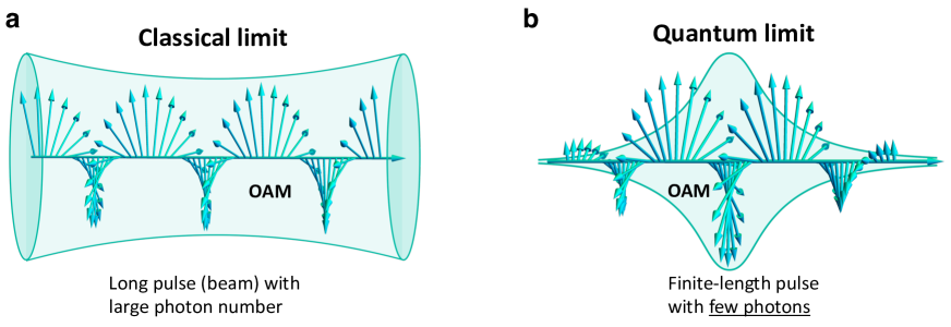
Figure 1: Schematic of a traditional twisted beam a compared to the quantum twisted pulse b put forth in this paper. The semi-classical theory only captures the mean angular momenta of a laser beam with large photon number. However, the quantum effects of photon statistics, vectorial uncertainty relations and non-local spin noise requires a new theoretical framework put forth in this paper.

In this work, we present a new frontier for quantum structured light involving twisted space-time wavepackets of light. We first construct the wave function of a quantum twisted pulse, as well as a twisted laser beam, from quantum field theory [32] instead of from the single-particle Schrödinger equation in the first-quantization picture [33, 34, 35]. By exploiting the recently discovered quantum operators of the angular momenta of light [36], we evaluate the mean value as well as the quantum uncertainty of the photon spin operator vector. Apart from the well-established global properties of polarization, we also investigate the quantum properties of the photon spin density vector, i.e., the spin texture, which is a function of space and time. We show that beyond the paraxial approximation, the photon spin density of a Bessel single-photon pulse can exhibit rich spatial texture. This builds on previous important work in the field but also marks a significant departure  [20, 21, 22, 31, 23, 24, 25, 26, 27, 28, 29, 30]. Our proposed framework provides a powerful and versatile tool to engineer the local photon spin and OAM densities of a quantum structured light pulse, specifically for spatiotemporal optical vortices [37, 38].

Non-local spin noise (i.e., spin density correlation) for electrons is a fundamental signature of quantum phases of magnetic condensed matter [39], specifically in new phases of matter such as quantum spin liquids without magnetic order [40]. However, no such quantum spin noise operator has been defined for photons till date. Our theoretical formalism allows us to overcome this challenge. Here, we introduce the quantum correlator of photonic spin density to characterize the nonlocal spin noise in light. This paves the way to explore new phases of light with long-range spin order.

We emphasize that our work immediately opens important experimental frontiers for exploration. We predict that for Bessel pulses with large OAM, there will exist large fluctuations in the OAM along orthogonal directions. This additional quantum noise can be verified in metrology experiments even with OAM laser beams. Recently, it was demonstrated that the nitrogen-vacancy (NV) center in diamond can be used as a quantum sensor for detecting the local spinning nature of photons [41]. The spin density of the off-resonant optical beam can induce an effective static magnetic field for the electron spin of the NV center, which itself is an atomic-scale magnetometer working at room temperature. Imaging of our discovered helical spin-density structure in this work can be realized with the same technology in the near future. Furthermore, our proposed non-local spin density correlation can also be measured in compound measurements with two or multiple NV centers.

Quantum Spin and orbital angular momenta of light

Recent work discovered the full quantum operator of the photon spin within quantum field theory  [36],

$$\hat{\bm{S}}=\frac{1}{c}\int d^{3}x\hat{\bm{\pi}}(\bm{r},t)\times\hat{\bm{A}}(\bm{r},t).$$ (1)

which obeys the canonical commutation relationships

$$[\hat{S}_{i},\hat{S}_{j}]=i\hbar\epsilon_{ijk}\hat{S}_{k},$$ (2)

where $\epsilon_{ijk}$ is the third-order Levi-Civita symbol. The directly observable quantities are $\hat{\bm{S}}^{\rm obs}=\varepsilon_{0}\int d^{3}r\hat{\bm{E}}_{\perp}(\bm{r},t)\times\hat{\bm{A}}_{\perp}(\bm{r},t)$ and $\hat{\bm{L}}^{\rm obs}=\varepsilon_{0}\int d^{3}r\hat{E}_{\perp}^{j}(\bm{r},t)(\bm{r}\times\bm{\nabla})\hat{A}_{\perp}^{j}(\bm{r},t)$, which are the spin and OAM angular momenta carried only by transversely polarized photons. Note, $\hat{\bm{E}}_{\perp}$ and $\hat{\bm{A}}_{\perp}$ are the transverse part of the electric field and the vector potential, respectively.

Using the circularly polarized plane waves, we can expand the observable photon spin and OAM operators as

$$\hat{\bm{S}}^{\rm obs} =\hbar\int d^{3}k\left[\hat{a}_{\bm{k},+}^{\dagger}\hat{a}_{\bm{k},+}-\hat{a}_{\bm{k},-}^{\dagger}\hat{a}_{\bm{k},-}\right]\bm{e}(\bm{k},3),$$ (3)

$$\hat{\bm{L}}^{\rm obs} =-i\hbar\int d^{3}k\sum_{\lambda=\pm}\hat{a}_{\bm{k},\lambda}^{\dagger}(\bm{k}\times\bm{\nabla}_{\bm{k}})\hat{a}_{\bm{k},\lambda},$$ (4)

where $\bm{e}(\bm{k},3)=\bm{k}/|\bm{k}|$ is the unit vector and $\lambda=\pm$ denote the left circular polarization (LCP) and right circular polarization (RCP) separately (see Supplementary Material). The ladder operators of the plane wave with wave vector $\bm{k}$ and polarization $\lambda$ satisfy the bosonic commutation relation $[\hat{a}_{\bm{k},\lambda},\hat{a}_{\bm{k}^{\prime},\lambda^{\prime}}^{\dagger}]=\delta(\bm{k}-\bm{k}^{\prime})\delta_{\lambda\lambda^{\prime}}$. The photon helicity is given by $\hat{\Lambda}=\hbar\int d^{3}k\left[\hat{a}_{\bm{k},+}^{\dagger}\hat{a}_{\bm{k},+}-\hat{a}_{\bm{k},-}^{\dagger}\hat{a}_{\bm{k},-}\right]$. We emphasize that the spin and OAM are separately observable due to the quantum commutation relations

$$[\hat{S}^{\rm obs}_{i},\hat{L}^{\rm obs}_{j}]=0.$$ (5)

To show the striking symmetry between the angular momentum of photons and electrons, we define a field operator for light in real space $\hat{\psi}(\bm{r})=[\hat{\psi}_{+}(\bm{r}),\hat{\psi}_{-}(\bm{r})]^{T}$, where

$$\hat{\psi}_{\lambda}(\bm{r})=\frac{1}{\sqrt{(2\pi)^{3}}}\int d^{3}k\hat{a}_{\bm{k},\lambda}e^{i\bm{k}\cdot\bm{r}}.$$ (6)

For the source-free case, our defined field operator in the Heisenberg picture satisfies the homogeneous wave equation

$$\left(\nabla^{2}-\frac{1}{c^{2}}\frac{\partial^{2}}{\partial t^{2}}\right)\hat{\psi}(\bm{r},t)=0.$$ (7)

Now, we can re-express the OAM and helicity operators of light in parallel to their electron counterparts

$$\hat{\bm{L}}^{{\rm obs}}=\int d^{3}r\hat{\psi}^{\dagger}(\bm{r})(\bm{r}\times\hat{\bm{p}})\hat{\psi}(\bm{r}),$$ (8)

and

$$\hat{\Lambda}=\int d^{3}r\hat{\psi}^{\dagger}(\bm{r})\hat{\sigma}_{z}\hat{\psi}(\bm{r})$$ (9)

where $\hat{\bm{p}}=-i\hbar\bm{\nabla}$ is momentum operator and $\hat{\sigma}_{z}=\rm{diag}[1,-1]$ is the Pauli matrix. However, similar expression for the spin operator $\hat{\bm{S}}^{\rm obs}$ can not be obtained in real space. The unit polarization vector $\bm{e}(\bm{k},3)$ in Eq. (59) for each plane wave is $\bm{k}$-dependent, i.e., dependent on its spatial momentum.

Quantum wave function of twisted light pulses

In previous sections, we have shown that both $\hat{\bm{S}}^{\rm obs}$ and $\hat{\bm{L}}^{\rm obs}$ are vector operators. However, in previous studies, usually only their projections on the propagating direction have been fully studied [20, 21, 31]. Their mean value on the transverse plane and more importantly, their quantum fluctuations have not been investigated. On the other hand, the near-field techniques have now been well developed. This makes it possible to measure and engineer the angular-momentum density of light, which is a vector function of space and time, in experiments. Thus, a fully quantum theory beyond the paraxial approximation to explore all classes of twisted pulses in a united framework is highly desirable. We now present this powerful theoretical tool by generalizing the quantum theory of continuous-mode field [32] to the twisted-pulse case.

We first define the single-photon wave-packet creation operator for a twisted photon pulse

$$\hat{a}_{\xi\lambda}^{\dagger}=\int d^{3}k\xi_{\lambda}(\bm{k})\hat{a}_{\bm{k}\lambda}^{\dagger},$$ (10)

as a coherent superposition of plane-wave modes. The pulse shape and other quantum properties of the pulse are fully determined by the spectral amplitude function (SAF) $\xi_{\lambda}(\bm{k})$. In the following, we denote the propagating direction of the pulse as the $z$-axis and work in the cylindrical coordinate in $k$-space $\bm{k}=k_{z}\bm{e}_{z}+\rho_{k}\bm{e}_{\rho}=\rho_{k}\cos\varphi_{k}\bm{e}_{x}+\rho_{k}\sin\varphi_{k}\bm{e}_{y}+k_{z}\bm{e}_{z}$. Here, $\rho_{k}$ is the radial distance from the $k_{z}$-axis, $\varphi_{k}$ is the azimuth angle, and $\bm{e}$ denotes the corresponding unit vector. The SAF of a twisted pulse with deterministic OAM can be generally expressed as

$$\xi_{\lambda}(\bm{k})=\frac{1}{\sqrt{2\pi}}\eta_{\lambda}(k_{z},\rho_{k})e^{im\varphi_{k}}.$$ (11)

Usually, the amplitude $\eta_{\lambda}(k_{z},\rho_{k})$ is symmetric in the transverse plane, i.e, it is independent on the azimuth angle $\varphi_{k}$. The phase factor $\exp(im\varphi_{k})$ with an integer $m$ will lead to the OAM of light in $z$-direction of a single-photon pulse as shown in the following.

The SAF is required to satisfy the normalization condition $\int d^{3}k\left|\xi_{\lambda}(\bm{k})\right|^{2}=1$. This guarantees that $\hat{a}_{\xi\lambda}^{\dagger}$ obeys the bosonic commutation relation

$$[\hat{a}_{\xi\lambda},\hat{a}_{\xi\lambda}^{\dagger}]=1.$$ (12)

Then, the wave-packet creation operator $\hat{a}_{\xi\lambda}^{\dagger}$ can be treated as a normal ladder operator of a harmonic oscillator. Using this commutation relation, we can construct the wave function of all classes of quantum pulses in the standard way, such as the most common $n$-photon Fock-state and coherent-state pulses [32, 42]

$$\left|n_{\xi\lambda}\right\rangle=\frac{1}{\sqrt{n!}}\left(\hat{a}_{\xi\lambda}^{\dagger}\right)^{n}\left|0\right\rangle,$$ (13)

and

$$\left|\alpha_{\xi\lambda}\right\rangle=\exp\left(\alpha\hat{a}_{\xi\lambda}^{\dagger}-\frac{1}{2}\bar{n}\right)\left|0\right\rangle=e^{-\bar{n}/2}\sum_{n=0}^{\infty}\frac{\alpha^{n}}{\sqrt{n!}}\left|n_{\xi\lambda}\right\rangle,$$ (14)

where $\bar{n}=|\alpha|^{2}$ is the mean photon number in the coherent-state pulse. The wave function of a squeezed-state pulse, an entangled two-photon pulse [43], or an ultra-short spatiotemporal vortex pulse [37, 38] can also be constructed similarly. Here, the polarization of the pulse is fixed as one of the circular polarizations. However, linearly or elliptically polarized quantum pulses can also be constructed with superposition of two circular polarization ladder operators $\hat{a}_{\xi\lambda}\ (\lambda=\pm)$. We also note that a twisted laser beam can be characterized by a wave function with a very long pulse length and very large photon number. Thus, our method also captures the cases of continuous OAM laser beams used widely in experiments.

Without loss of generality, we only take the Bessel pulses as an example to show the quantum properties of the spin and OAM of twisted pulses. Other twisted pulses, such as a Bessel-Gaussian or Laguerre-Gaussian pulse, can be treated similarly. The single-frequency Bessel beam is the superposition of all plane waves on the cone with the same frequency $\omega=c|\bm{k}|$, $k_{z}$, and polar angle $\theta_{k}=\theta_{c}$ as shown in Fig. 2. Then, the SAF of a Bessel pulse with a Gaussian envelope can be expressed $\eta_{\lambda}(k_{z},\rho_{k})$ as the product of two Gaussian functions

$$\eta_{\lambda}(k_{z},\rho_{k})= \left(\frac{2\sigma_{z}^{2}}{\pi}\right)^{1/4}\exp\left[-\sigma_{z}^{2}(k_{z}-k_{z,c})^{2}\right]$$

$$\times\left(\frac{2\sigma_{\rho}^{2}}{\pi k_{\perp,c}^{2}}\right)^{1/4}\exp\left[-\sigma_{\rho}^{2}(\rho_{k}-k_{\perp,c})^{2}\right].$$ (15)

The first Gaussian function with width $1/\sigma_{z}$ and center wave vector $k_{z,c}$ characterizes the envelope of the pulse in the propagating direction. The pulse length on $z$-axis in real space is given by $\sigma_{z}=c\tau_{p}$ ($\tau_{p}$ the pulse length in time domain). Distinct from previous works [27, 44], we do not add a delta function [such as $\delta(\theta_{k}-\theta_{c})$] in the SAF to characterize its distribution property in the $xy$-plane. This will cause a serious issue that the wave functions of the quantum pulses cannot be normalized, because $\int d^{3}k|\xi_{\lambda}(\bm{k})|^{2}\propto\delta(\theta_{k}-\theta_{c})$. Instead, we utilize another Gaussian function with width $1/\sigma_{\rho}$ and center value $k_{\perp,c}=k_{z,c}\tan\theta_{c}$. These two Gaussian functions should have the same ratio between center wave-number and the width, i.e. $k_{z,c}\sigma_{z}=k_{\perp,c}\sigma_{\rho}\equiv C_{0}$. In the narrow bandwidth limit $C_{0}\gg 1$, our defined SAF is well normalized [42]. We also note that in contrast to the Bessel-mode-based method [28] which only applies to Bessel beams, our generalized plane-wave-based framework is amenable to unify the theory of all classes of quantum pulses.

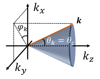
Figure 2: Schematic of the spectral distribution of a Bessel beam.

Quantum statistics of the photon spin

Traditionally, the angular momentum carried by each photon in a twisted laser beam has been calculated semi-classically via the ratio of angular flux to the energy flux [20, 21] and only its projection on the propagating axis has been studied. Although the projection of the photon spin and OAM of a non-paraxial beam on the transverse plane has caused attention recently [31, 22, 23, 24, 26], a systematic and comprehensive investigation of the vector nature of the photon spin and OAM is still missing. Specifically, the Heisenberg uncertainty relation for photon OAM has never been investigated. On the other hand, many researchers have also tried to establish a quantum theory of the angular momentum of light in the last two decades [27, 28, 29, 30]. However, a fully quantum framework to handle arbitrary quantum pulses beyond the paraxial approximation has not been found.

We first calculate the mean value of the spin of a Fock-state Bessel pulse with polarization $\lambda$ and photon number $n$,

$$\left\langle n_{\xi\lambda}\right|\hat{\bm{S}}^{{\rm obs}}\left|n_{\xi\lambda}\right\rangle=\hbar n\lambda\left(0,0,\cos\theta_{c}\right).$$ (16)

Here, we see that the magnitude of the spin carried by each circularly polarized photon is usually smaller than $\hbar$ and approaches to $\hbar$ asymptotically in the paraxial limit ( $\theta_{c}\rightarrow 0$) [27, 23]. This is significantly different from the helicity, which is exactly $\hbar$. If the SAF of a pulse is symmetric in the $xy$-plane, then the mean value of the spin in the $xy$-plane vanishes, i.e., $\langle\hat{S}^{\rm obs}_{x}\rangle=\langle\hat{S}^{\rm obs}_{y}\rangle=0$. However, we show that the quantum fluctuations of photon spin in the $xy$-plane is not zero. The standard derivations of the spin of an $n$-photon Fock-state Bessel pulse are given by

$$\Delta\hat{S}^{\rm obs}_{x}=\Delta\hat{S}^{\rm obs}_{y}=\hbar\sqrt{n/2}\left|\sin\theta_{c}\right|,\ \Delta\hat{S}^{\rm obs}_{z}=0.$$ (17)

This is significantly beyond the previous semi-classical theory [20, 21, 31], in which the quantum statistics of the photon spin cannot be studied.

Similarly, we can evaluate the mean value of the spin of a coherent-state Bessel pulse with polarization $\lambda$ and photon number $\bar{n}=|\alpha|^{2}$,

$$\left\langle\alpha_{\xi\lambda}\right|\hat{\bm{S}}^{\rm obs}\left|\alpha_{\xi\lambda}\right\rangle=\hbar\bar{n}\lambda\left(0,0,\cos\theta_{c}\right).$$ (18)

Here, we see that the average spin carried by each photon is still $\hbar\cos\theta_{c}$ and the spin’s projection on $xy$-plane also vanishes. However, the quantum statistics of the photon spin for a coherent-state pulse is significantly different from that of a Fock-state pulse,

$$\Delta\hat{S}^{\rm obs}_{x}=\Delta\hat{S}^{\rm obs}_{y}=\hbar\sqrt{\bar{n}/2}\left|\sin\theta_{c}\right|,\ \Delta\hat{S}^{\rm obs}_{z}=\bar{n}\hbar\left|\cos\theta_{c}\right|.$$ (19)

The Poisson statistics of a coherent pulse leads to non-vanishing $\Delta\hat{S}^{\rm obs}_{z}$ in contrast to a sub-Poisson Fock-state pulse.

Figure 3: Photonic OAM fluctuation in the transverse plane. a OAM measurements in the direction orthogonal to the propagating $z$-axis. A Bessel pulse has vanishing mean OAM in $xy$-plane but non-zero OAM fluctuations, $(\Delta\hat{L}_{x}^{\rm obs})^{2}=(\Delta\hat{L}_{y}^{\rm obs})^{2}\neq 0$. b The quantum uncertainty of $\hat{L}_{x}^{\rm obs}$ is linearly proportional to the photon number $n$ in the pulse. Different lines correspond to different the helical phase index $m$. c The quantum uncertainty of $\hat{L}_{x}^{\rm obs}$ is proportional to the square of $m$. d The OAM fluctuation in $xy$-plane is strongly dependent on the polar angle $\theta_{c}$ of a Bessel pulse. The ratio $C_{0}$ has been taken as $100$ in all simulations.

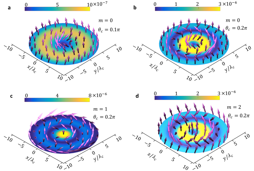
Figure 4: Spin texture of a single-photon LCP Bessel pulse on the pulse-center plane with $k_{z,c}z=ct$. (a-d) correspond to different quantum numbers $m$ and polar angles $\theta_{c}$. The colorbar describes the amplitude of spin density in unit of $\hbar/\lambda^{3}_{c}$.

Quantum statistics of the photon OAM

Heisenberg’s uncertainty relation is the canonical quantum characteristics of angular momentum. However, this relation for photon OAM has never been addressed till date. Here, we present a quantitative investigation about the quantum statistics of photon OAM. We discover that for beams with large OAM number, there exist large fluctuations for the OAM operators in the orthogonal directions i.e. in the transverse plane. This quantum effect can be observed in experiment even with traditional OAM laser beams. The mean value of $\hat{L}^{\rm obs}_{z}$ for a Fock-state twisted pulse with photon number $n$ is given by,

$$\left\langle n_{\xi\lambda}\right|\!\hat{L}^{\rm obs}_{z}\!\left|n_{\xi\lambda}\right\rangle\!=\! -\frac{in\hbar}{2\pi}\!\!\int\!\!d^{3}k\eta_{\lambda}(\bm{k})e^{-im\varphi_{k}}\!\frac{\partial}{\partial\varphi_{k}}\!\eta_{\lambda}(\bm{k})e^{im\varphi_{k}}$$ (20)

$$= mn\hbar.$$ (21)

This reduces to the well-known result obtained from the semi-classical method that each twisted photon carries $m\hbar$ OAM [20, 21]. We see that $\langle\hat{L}^{\rm obs}_{z}\rangle$ is independent on the photon polarization. It is only determined by the photon number $n$ and integer $m$ in the helical phase factor $\exp(im\varphi_{k})$ if $\eta_{\lambda}(\bm{k})$ is not a function of $\varphi_{k}$. We can also verify that, in this case, the mean value of photon OAM in $xy$-plane vanishes, i.e., $\langle\hat{L}^{\rm obs}_{x}\rangle=\langle\hat{L}^{\rm obs}_{y}\rangle=0$ (see Supplementary Material).

The quantum variances of the three components of photon OAM for a Fock-state Bessel pulse are given by (please refer to the Supplementary Material for details)

$$(\Delta\hat{L}^{\rm obs}_{z})^{2}\!=\!\left\langle n_{\xi\lambda}\right|(\hat{L}^{\rm obs}_{z})^{2}\left|n_{\xi\lambda}\right\rangle\!-\!\left\langle n_{\xi\lambda}\right|\hat{L}^{\rm obs}_{z}\left|n_{\xi\lambda}\right\rangle^{2}\!=\!0,$$ (22)

and

$$(\Delta\hat{L}^{\rm obs}_{x})^{2}=(\Delta\hat{L}^{\rm obs}_{y})^{2}$$

$$=\frac{1}{2}n\hbar^{2}\left[\left(C_{0}^{2}+\frac{1}{4}\right)x^{2}+\left(C_{0}^{2}+m^{2}+\frac{3}{4}\right)\frac{1}{x^{2}}-1\right]$$ (23)

$$\geq\frac{1}{2}n\hbar^{2}\left[\sqrt{(4C_{0}^{2}+1)(C_{0}^{2}+m^{2}+\frac{3}{4})}-1\right]\gg\frac{1}{2}mn\hbar^{2},$$ (24)

where $x=\tan\theta_{c}\in(0,\infty)$ and we have used the inequality relation $a^{2}x^{2}+b^{2}/x^{2}\geq 2|ab|$ and the narrow-band condition $C_{0}\gg 1$. This immediately leads to the Heisenberg relation

$$\sqrt{(\Delta\hat{L}^{\rm obs}_{x})^{2}(\Delta\hat{L}^{\rm obs}_{y})^{2}}>\frac{\hbar}{2}\left|\langle\hat{L}_{z}\rangle\right|=\frac{1}{2}mn\hbar^{2}.$$ (25)

The other two Heisenberg relations for photon OAM are trivial due to the vanishing mean values of $\hat{L}^{\rm obs}_{x}$ and $\hat{L}^{\rm obs}_{y}$. Similar results also hold for a coherent-state twisted pulse, but with non-vanishing $(\Delta\hat{L}^{\rm obs}_{z})^{2}=\hbar^{2}\bar{n}m^{2}$.

Our predicted large OAM fluctuations in $xy$-plane can be verified in experiments (see Fig. 3a). The quantum uncertainties of $\hat{L}_{x}^{\rm obs}$ and $\hat{L}_{y}^{\rm obs}$ are linearly proportional to the photon number $n$ in a Bessel pulse as shown in Fig. 3b and proportional to the square of the helical phase index $m$ in Eq. (11) as shown in  3c. From Eq. (23), we see that the OAM fluctuations in the transverse plane is strongly dependent on the polar angle $\theta_{c}$ of a Bessel pulse. There exists a minimum-uncertainty angle due to the inequality $a^{2}x^{2}+b^{2}/x^{2}\geq 2|ab|$ ($x=\tan\theta_{c}$) in (24) as shown in  3d. For a optical pulse, the ratio $C_{0}$ between its center wave number and its width is usually very large, e.g., $C_{0}\approx 188$ for a $50$ fs pulse with center wave length $\lambda_{c}=500$ nm. In our numerical simulation, we set $C_{0}=100$. We note that this large OAM fluctuations in the transverse plane also exist in traditional OAM laser beams, such as the routinely used Laguerre-Gaussian beams in experiments.

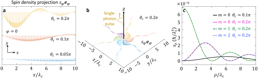
Figure 5: Projections of the spin density of a Bessel single-photon pulse on $xy$-plane (panel a and b) and on $z$-axis in panel c. Panel a corresponds to the case with fixed azimuthal angle $\phi=0$, but different polar angle $\theta_{c}$. Panel b corresponds to the case with fixed polar angle $\theta_{c}=0.2\pi$, but different azimuthal angle $\phi=\{0,\pi/3,2\pi/3,\pi,4\pi/3,5\pi/3\}$. Panel c shows the $z$-component of the spin density.

Quantum spin texture of a single-photon pulse

We show that the spin texture of a single-photon pulse can exhibit a very rich and interesting structure in the case beyond the paraxial approximation. The photon spin texture is characterized by the spin density operator

$$\hat{\bm{s}}^{\rm obs}(\bm{r},t)=\varepsilon_{0}\hat{\bm{E}}_{\perp}(\bm{r},t)\times\hat{\bm{A}}_{\perp}(\bm{r},t).$$ (26)

Similar to the electric or magnetic fields, the spin density can be treated as a vector field and can be measured locally [41]. We emphasize that as a vector, the spin density is neither purely longitudinal or purely transverse in most cases. In the single-mode plane-wave limit, the spin density will be a space-independent constant, i.e., $\bm{\nabla}\times\langle\hat{\bm{s}}^{\rm obs}(\bm{r},t)\rangle=\bm{\nabla}\cdot\langle\hat{\bm{s}}^{\rm obs}(\bm{r},t)\rangle=0$.

The mean value of the spin density of a Fock-state Bessel pulse is given

$$\left\langle n_{\xi\lambda}\right|\hat{\bm{s}}^{\rm obs}(\bm{r},t)\left|n_{\xi\lambda}\right\rangle=\lambda\left(s_{\varphi}\bm{e}_{\varphi}+s_{z}\bm{e}_{z}\right),$$ (27)

where

$$s_{z} =\frac{n\hbar C_{0}}{2\pi\sigma_{z}\sigma_{\rho}^{2}}\left\{\left[J_{m-\lambda}(k_{\perp,c}\rho)\right]^{2}\cos^{4}\frac{\theta_{c}}{2}-\left[J_{m+\lambda}(k_{\perp,c}\rho)\right]^{2}\sin^{4}\frac{\theta_{c}}{2}\right\}\exp\left[-\frac{\left(ct-z\cos\theta_{c}\right)^{2}}{2\sigma_{z}^{2}\cos^{2}\theta_{c}}\right],$$ (28)

and

$$s_{\varphi} =\frac{n\hbar C_{0}\sin\theta_{c}}{2\pi\sigma_{z}\sigma_{\rho}^{2}}\left[\cos^{2}\frac{\theta_{c}}{2}J_{m}(k_{\perp,c}\rho)J_{m-\lambda}(k_{\perp,c}\rho)+\sin^{2}\frac{\theta_{c}}{2}J_{m+\lambda}(k_{\perp,c}\rho)J_{m}(k_{\perp,c}\rho)\right]\exp\left[-\frac{\left(ct-z\cos\theta_{c}\right)^{2}}{2\sigma_{z}^{2}\cos^{2}\theta_{c}}\right],$$ (29)

with $\bm{r}=\rho\bm{e}_{\rho}+z\bm{e}_{z}$. The spin density of a coherent pulse can be evaluated similarly. Here, we can see the following key characters of the spin density: (i) its projection in the $xy$-plane is symmetric around $z$-axis. This causes the corresponding spatial integral to vanish as shown in previous section, i.e., $\langle\hat{S}^{\rm obs}_{x}\rangle=\langle\hat{S}^{\rm obs}_{y}\rangle=0$; (ii) its $xy$-plane projection is parallel or anti-parallel to the azimuth-angle-dependent unit vector $\bm{e}_{\varphi}$ and it does not have a radial component. This leads to the helical spin texture as shown in Fig. 4. (iii) its $xy$-plane projection contains the product of two different Bessel functions, which can lead to the oscillation between clockwise and anti-clockwise structures; (iv) its projection on $z$ is independent on $\varphi$. For a small angle $\theta_{c}$, the term $\sim\cos^{4}(\theta_{c}/2)$ dominates. Thus, the sign of $s_{z}$ is always positive (negative) for LCP (RCP) pulse. This leads to the non-vanishing global spin $\langle\hat{S}_{M,z}\rangle$.

We show the spin texture of an LCP single-photon ($n=1$) Fock-state Bessel pulse in Fig. 4. Here, we only look at the spin density vector field on the plane $k_{z,c}z=ct$, at which the Gaussian functions in Eqs. (28) and (29) reach their maxima. In this case, the space-dependent spin density is only a function of the radius $\rho$ and the azimuthal angle $\varphi$ contained in $\bm{e}_{\varphi}$. For a pulse with small polar angle $\theta_{c}=0.1\pi$, almost only a clockwise structure can be observed in panel a. However, for a pulse with larger polar angle $\theta_{c}=0.2\pi$, the oscillation between clockwise and counter-clockwise structure can be observed clearly. This oscillation can only be obtained beyond the scalar-field theory and the paraxial approximation. For higher-order Bessel pulses with $m>0$, the fine structure of the spin density is significantly different from the $m=0$ case. The innermost ring changes from clockwise to counter-clockwise as shown in panel c and panel d. We also note that the Bessel pulse with $m=1$ is very special (see panel c), because the spin texture has a peak instead of a hole at the center.

In Fig. 5, we show more details of the projection of the spin density vector field on $xy$-plane and $z$-axis, respectively. In panel a, we look at the projection of the spin density on $xy$-plane $s_{\varphi}\bm{e}_{\varphi}$ with fixed Bessel order index as $m=0$ and the azimuthal angle as $\varphi=0$ (i.e., along the $x$-axis). For a pulse with small $\theta_{c}$ (see the blue arrows at the bottom), $s_{\varphi}\bm{e}_{\varphi}$ is relatively small and flat. The amplitude of $s_{\varphi}$ decrease with $\theta_{c}$ and it vanishes when $\theta_{c}\rightarrow 0$. For a pulse with larger $\theta_{c}$ (see the yellow arrows at the top), the sign of $s_{\varphi}$ oscillates between $\pm 1$ with increasing $\rho$. This explains the oscillation between the clockwise and counter-clockwise structure shown in Fig. 4 b. In panel b, we show the rotation of $s_{\varphi}\bm{e}_{\varphi}$ in $xy$-plane with fixed $m=0$ and $\theta_{c}=0.2\pi$. In panel c, we show the projection of the spin density on $z$-axis as the function of $\rho$ for the four cases in Fig. 4. Here, we clearly see the oscillation induced by the Bessel function in Eq. (28). Specifically, the vertex at the center for $m=1$.

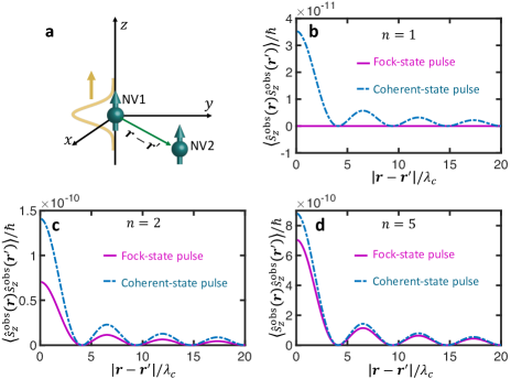
Figure 6: Non-local spin noise. a Our proposed spin density correlation measurement with two nitrogen-vacancy centers at $\bm{r}$ and $\bm{r}^{\prime}$, respectively. b-d Contrast of spin density correlation between Fock-state and coherent-state pulses. Here, $n$ is the mean photon number in each pulse and we show the results for the case with $m=1$ and $\theta_{c}=0.2\pi$. One of the quantum sensor is fixed on the $z$-axis and the other sensor can move in $xy$-plane.

Nonlocal spin noise of light

To characterize the nonlocal spin noise of light, we introduce the quantum correlation function of the photon spin density. Due to the vector nature of the spin density, the full two-point correlation should be characterized by a $3\times 3$ correlation matrix as shown in the supplementary. Here, we only describe the equal-time correlator $\left\langle\hat{s}^{\rm obs}_{z}(\bm{r},t)\hat{s}^{\rm obs}_{z}(\bm{r}^{\prime},t)\right\rangle$.

In the paraxial limit ($\theta_{c}\approx 0$), the two-point correlation functions for a Fock-state and a coherent-state pulse are given by

$$\left\langle n_{\xi\lambda}\right|\hat{s}^{\rm obs}_{z}(\bm{r},t) \hat{s}^{\rm obs}_{z}(\bm{r}^{\prime},t)\left|n_{\xi\lambda}\right\rangle\approx\hbar^{2}\left[\delta(\bm{r}-\bm{r}^{\prime})n\left|\psi_{-\lambda}(\bm{r},t)\right|^{2}\right.$$

$$\left.\ \ \ +n(n-1)\left|\psi_{-\lambda}(\bm{r},t)\right|^{2}\left|\psi_{-\lambda}(\bm{r}^{\prime},t)\right|^{2}\right],$$ (30)

and

$$\left\langle\alpha_{\xi\lambda}\right|\hat{s}^{\rm obs}_{z}(\bm{r},t)\hat{s}^{\rm obs}_{z} (\bm{r}^{\prime},t)\left|\alpha_{\xi\lambda}\right\rangle\approx\hbar^{2}\left[\delta(\bm{r}-\bm{r}^{\prime})\bar{n}\left|\psi_{-\lambda}(\bm{r},t)\right|^{2}\right.$$

$$\left.+\bar{n}^{2}\left|\psi_{-\lambda}(\bm{r},t)\right|^{2}\left|\psi_{-\lambda}(\bm{r}^{\prime},t)\right|^{2}\right],$$ (31)

where

$$\psi_{\lambda}(\bm{r},t)=\frac{1}{\sqrt{(2\pi)^{3}}}\int d^{3}k\xi_{\lambda}(\bm{k})e^{i[(\bm{k}\cdot\bm{r}-\omega)t+\lambda\varphi_{k}]},$$ (32)

is the effective wave function of a pulse in real space. This method can be easily generalized to higher-order correlations.

We note that the delta function $\delta(\bm{r}-\bm{r}^{\prime})$ in the correlation function will not lead to any diverging effect, because a practical probe always measures the averaged photon spin density over a finite volume instead of the true single-point spin density. On the other hand, this term vanishes in a composite measurement with $\bm{r}\neq\bm{r}$. In this case, we see that the Poisson and sub-Poisson statistics automatically enter the quantum spin-density correlations. Specifically, the two-point spin density correlation vanishes for a single-photon Fock-state pulse as expected.

We now propose to detect the non-local spin density correlation via compound measurements of two NV centers, which have been exploited as nano-scale quantum sensors for photonic spin density measurements recently [41]. As shown in Fig. 6a, we fixed one quantum sensor on the $z$-axis and move the other one to image the distribution of the spin density correlation in the transverse plane. We contrast the spin density correlations in Fock-state and coherent-state Bessel pules in Fig. 6b-d. Here, we see that in the few-photon limit, there exist significant differences between Fock-state and coherent pulses. This difference fundamentally roots in the quantum statistics of photons and it will disappear in the large-photon limit.

Currently, imaging of single-photon level spin density and the corresponding correlation is extremely challenging in experiments. However, our discovered interesting texture of spin density and non-local spin noise also exists in traditional OAM beam, which can be demonstrated in the near future. On the other hand, due to the absence of photon-photon interaction, the nonlocal spin noise within a light pulse in free space is fully determined by the photon-number statistics. However, we predict that exotic photonic phases with long-range spin order can exist in a quantum polariton system or an atomic lattice [45, 46].

Conclusion

We have established the fully quantum framework for photonic angular momenta of quantum structured pulses, as well as the corresponding quantum texture. Our approach presents a paradigm shift for the photonics community as it can be exploited to study the quantum properties and to reveal the vector nature of angular momentum of light. We have shown that the spin texture of a Bessel pulse can exhibit very interesting structure beyond the paraxial limit. Our proposed non-local spin noise will open a new frontier for studying exotic phases of photons with long-range spin order. This spin noise can be measured in compound measurements with multiple nanoscale spin sensors, which have been proposed and demonstrated in our previous experiment [41].

Supplementary Materials for “Quantum structured light: Non-classical spin texture of twisted single-photon pulses”

I Quantum operator of photon angular momentum and helicity

In this section, we give the quantum operators of the photon angular momentum. First, we give the plane-wave expansion of the electromagnetic (EM) field operators in free space

$$\hat{\bm{A}}_{\perp}(\bm{r},t) =\int d^{3}k\sum_{\lambda=1}^{2}\sqrt{\frac{\hbar}{2\varepsilon_{0}\omega(2\pi)^{3}}}\left[\hat{a}_{\bm{k},\lambda}\bm{e}(\bm{k},\lambda)e^{i(\bm{k}\cdot\bm{r}-\omega t)}+{\rm h.c.}\right],$$ (33)

$$\hat{\bm{E}}_{\perp}(\bm{r},t) =i\int d^{3}k\sum_{\lambda=1}^{2}\sqrt{\frac{\hbar\omega}{2\varepsilon_{0}(2\pi)^{3}}}\left[\hat{a}_{\bm{k},\lambda}\bm{e}(\bm{k},\lambda)e^{i(\bm{k}\cdot\bm{r}-\omega t)}-{\rm h.c.}\right],$$ (34)

$$\hat{\bm{B}}(\bm{r},t) =\frac{i}{c}\int d^{3}k\sqrt{\frac{\hbar\omega}{2\varepsilon_{0}(2\pi)^{3}}}\left\{\left[\hat{a}_{\bm{k},1}\bm{e}(\bm{k},2)-\hat{a}_{\bm{k},2}\bm{e}(\bm{k},1)\right]e^{i(\bm{k}\cdot\bm{r}-\omega t)}-{\rm h.c.}\right\},$$ (35)

where $\varepsilon_{0}$ is the vacuum permittivity, $\omega=c|\bm{k}|$ is the frequency of the mode with wave vector $\bm{k}$ and $\bm{e}(\bm{k},\lambda)$ ($\lambda=1,2$) are the unit polarization vectors of the two transverse modes for each $\bm{k}$, i.e., $\bm{e}(\bm{k},1)\cdot\bm{k}=\bm{e}(\bm{k},2)\cdot\bm{k}=\bm{e}(\bm{k},1)\cdot\bm{e}(\bm{k},2)=0$. Here, we works in the Heisenberg picture, thus all field operators are time-dependent.

Using the bosonic commutation relations for the ladder operators

$$[\hat{a}_{\bm{k},\lambda},\hat{a}_{\bm{k}^{\prime},\lambda^{\prime}}^{\dagger}]=\delta(\bm{k}-\bm{k}^{\prime})\delta_{\lambda,\lambda^{\prime}},\ [\hat{a}_{\bm{k},\lambda},\hat{a}_{\bm{k}^{\prime},\lambda^{\prime}}]=[\hat{a}_{\bm{k},\lambda}^{\dagger},\hat{a}_{\bm{k}^{\prime},\lambda^{\prime}}^{\dagger}]=0,$$ (36)

we can verify the following equal-time commutation relations

$$[\hat{A}_{\perp}^{i}(\bm{r},t),\hat{E}^{j}_{\perp}(\bm{r}^{\prime},t)]=-\frac{i\hbar}{\varepsilon_{0}}\delta(\bm{r}-\bm{r}^{\prime})\delta^{\perp}_{ij},\ [\hat{A}_{\perp}^{i}(\bm{r},t),\hat{A}^{j}_{\perp}(\bm{r}^{\prime},t)]=[\hat{E}_{\perp}^{i}(\bm{r},t),\hat{E}^{j}_{\perp}(\bm{r}^{\prime},t)]=0,$$ (37)

where we have used the identity $\sum_{\lambda=1,2}e_{i}(k,\lambda)e_{j}(k,\lambda)=\delta^{\perp}_{ij}$.

In our previous work [36], we discovered the quantum operator of the full photon spin,

$$\hat{\bm{S}}=\frac{1}{c}\int d^{3}x\hat{\bm{\pi}}(\bm{r},t)\times\hat{\bm{A}}(\bm{r},t).$$ (38)

We have shown that the well-known spin and orbital angular momentum (OAM) of light

$$\hat{\bm{S}}^{\rm obs} =\varepsilon_{0}\int d^{3}r\hat{\bm{E}}_{\perp}(\bm{r},t)\times\hat{\bm{A}}_{\perp}(\bm{r},t)=i\hbar\int d^{3}k\left[\hat{a}_{\bm{k},2}^{\dagger}\hat{a}_{\bm{k},1}-\hat{a}_{\bm{k},1}^{\dagger}\hat{a}_{\bm{k},2}\right]\bm{e}(\bm{k},3),$$ (39)

$$\hat{\bm{L}}^{\rm obs} =\varepsilon_{0}\int d^{3}r\hat{E}_{\perp}^{j}(\bm{r},t)(\bm{r}\times\bm{\nabla})\hat{A}_{\perp}^{j}(\bm{r},t)=-i\hbar\int d^{3}k\sum_{\lambda=1,2}\hat{a}_{\bm{k},\lambda}^{\dagger}(\bm{k}\times\bm{\nabla}_{\bm{k}})\hat{a}_{\bm{k},\lambda},$$ (40)

are the directly observable part of photon angular momentum. Here, $\bm{e}(\bm{k},3)=\bm{k}/|\bm{k}|$ is the unit vector in the propagating direction of each mode. In this paper, we will only study the observable part of photon angular momentum $\hat{\bm{S}}^{\rm obs}$ and $\hat{\bm{L}}^{\rm obs}$, which both are gauge invariant. The helicity of the photon is defined as

$$\hat{\Lambda}=i\hbar\int d^{3}k\left[\hat{a}_{\bm{k},2}^{\dagger}\hat{a}_{\bm{k},1}-\hat{a}_{\bm{k},1}^{\dagger}\hat{a}_{\bm{k},2}\right],$$ (41)

which is a Lorentz invariant scalar.

We emphasize that there exist significant differences between the spin and OAM of photons. The photon spin angular momentum fundamentally originates from the rotation between different polarization modes, which generates the relative phase between the plane-wave modes with the same momentum $\bm{k}$. However, the OAM roots in the extrinsic spatial rotation fully, which generates the relative phase between plane-wave modes with different momentum $\bm{k}$, but with the same polarization $\lambda$. This explains that $\hat{\bm{S}}^{\rm obs}$ and $\hat{\bm{L}}^{\rm obs}$ can still be measured independently even though photons do not have intrinsic spin degrees of freedom.

I.1 Commutation relations

Now, we check the commutation relations between the angular momenta of light. This can be done much more easily in the k-space. We first check the photon spin

$$[\hat{S}^{\rm obs}_{i},\hat{S}^{\rm obs}_{j}] =-\hbar^{2}\int d^{3}k\int d^{3}k^{\prime}\left[\hat{a}_{\bm{k},2}^{\dagger}\hat{a}_{\bm{k},1}-\hat{a}_{\bm{k},1}^{\dagger}\hat{a}_{\bm{k},2},\hat{a}_{\bm{k}^{\prime},2}^{\dagger}\hat{a}_{\bm{k}^{\prime},1}-\hat{a}_{\bm{k}^{\prime},1}^{\dagger}\hat{a}_{\bm{k}^{\prime},2}\right]e_{i}(\bm{k},3)e_{j}(\bm{k}^{\prime},3)$$ (42)

$$=\hbar^{2}\int d^{3}k\int d^{3}k^{\prime}\left(\hat{a}_{\bm{k},2}^{\dagger}\hat{a}_{\bm{k},2}-\hat{a}_{\bm{k},1}^{\dagger}\hat{a}_{\bm{k},1}+\hat{a}_{\bm{k},1}^{\dagger}\hat{a}_{\bm{k},1}-\hat{a}_{\bm{k},2}^{\dagger}\hat{a}_{\bm{k},1}\right)\delta(\bm{k}-\bm{k}^{\prime})e_{i}(\bm{k},3)e_{j}(\bm{k}^{\prime},3)$$ (43)

$$=0.$$ (44)

This recovers the result obtained by van Enk and Nienhuis in 1994 [47, 48]. For the photon OAM operator, we have

$$[\hat{L}^{\rm obs}_{i},\hat{L}^{\rm obs}_{j}]= -\hbar^{2}\int d^{3}k\int d^{3}k^{\prime}\sum_{\lambda,\lambda^{\prime}=1,2}\left[\hat{a}_{\bm{k},\lambda}^{\dagger}(\bm{k}\times\bm{\nabla}_{\bm{k}})_{i}\hat{a}_{\bm{k},\lambda},\hat{a}_{\bm{k}^{\prime},\lambda^{\prime}}^{\dagger}(\bm{k}^{\prime}\times\bm{\nabla}_{\bm{k}^{\prime}})_{j}\hat{a}_{\bm{k}^{\prime},\lambda^{\prime}}\right]$$ (45)

$$= -\hbar^{2}\!\!\int\!\!d^{3}k\!\!\int\!\!d^{3}k^{\prime}\!\!\sum_{\lambda,\lambda^{\prime}=1,2}\!\left\{\hat{a}_{\bm{k},\lambda}^{\dagger}(\bm{k}\times\bm{\nabla}_{\bm{k}})_{i}\delta(\bm{k}-\bm{k}^{\prime})\delta_{\lambda\lambda^{\prime}}(\bm{k}^{\prime}\times\bm{\nabla}_{\bm{k}^{\prime}})_{j}\hat{a}_{\bm{k}^{\prime},\lambda^{\prime}}-\hat{a}_{\bm{k}^{\prime},\lambda^{\prime}}^{\dagger}(\bm{k}^{\prime}\times\bm{\nabla}_{\bm{k}^{\prime}})_{j}\delta(\bm{k}-\bm{k}^{\prime})\delta_{\lambda\lambda^{\prime}}(\bm{k}\times\bm{\nabla}_{\bm{k}})_{i}\hat{a}_{\bm{k},\lambda}\right\}$$ (46)

$$= -\hbar^{2}\int d^{3}k\sum_{\lambda=1,2}\hat{a}_{\bm{k},\lambda}^{\dagger}\left[(\bm{k}\times\bm{\nabla}_{\bm{k}})_{i}(\bm{k}\times\bm{\nabla}_{\bm{k}})_{j}-(\bm{k}\times\bm{\nabla}_{\bm{k}})_{j}(\bm{k}\times\bm{\nabla}_{\bm{k}})_{i}\right]\hat{a}_{\bm{k},\lambda}$$ (47)

$$= \hbar^{2}\int d^{3}k\sum_{\lambda=1,2}\hat{a}_{\bm{k},\lambda}^{\dagger}\epsilon_{ijk}(\bm{k}\times\bm{\nabla}_{\bm{k}})_{k}\hat{a}_{\bm{k},\lambda}=i\hbar\epsilon_{ijk}\hat{L}^{\rm obs}_{k},$$ (48)

where we have used the identity

$$(\bm{k}\times\bm{\nabla}_{\bm{k}})_{i}(\bm{k}\times\bm{\nabla}_{\bm{k}})_{j}-(\bm{k}\times\bm{\nabla}_{\bm{k}})_{j}(\bm{k}\times\bm{\nabla}_{\bm{k}})_{i}=-\epsilon_{ijk}(\bm{k}\times\bm{\nabla}_{\bm{k}})_{j}.$$ (49)

Different from previous studies [47, 48, 27, 29], we show that $\hat{\bm{L}}^{\rm obs}$ satisfies the canonical angular momentum commutation relations. More importantly, we show that the spin and OAM of light commute with each other

$$[\hat{S}^{\rm obs}_{i},\hat{L}^{\rm obs}_{j}] =\hbar^{2}\int d^{3}k\int d^{3}k^{\prime}e_{i}(\bm{k},3)\sum_{\lambda^{\prime}=1,2}[\hat{a}_{\bm{k},2}^{\dagger}\hat{a}_{\bm{k},1}-\hat{a}_{\bm{k},1}^{\dagger}\hat{a}_{\bm{k},2},\hat{a}_{\bm{k}^{\prime},\lambda^{\prime}}^{\dagger}(\bm{k}^{\prime}\times\bm{\nabla}_{\bm{k}^{\prime}})_{j}\hat{a}_{\bm{k}^{\prime},\lambda^{\prime}}]$$ (50)

$$=\hbar^{2}\int d^{3}ke_{i}(\bm{k},3)\left\{\hat{a}_{\bm{k},2}^{\dagger}(\bm{k}\times\bm{\nabla}_{\bm{k}})_{j}\hat{a}_{\bm{k},1}-\hat{a}_{\bm{k},2}^{\dagger}(\bm{k}\times\bm{\nabla}_{\bm{k}})_{j}\hat{a}_{\bm{k},1}-\hat{a}_{\bm{k},1}^{\dagger}(\bm{k}\times\bm{\nabla}_{\bm{k}})_{j}\hat{a}_{\bm{k},2}+\hat{a}_{\bm{k},1}^{\dagger}(\bm{k}\times\bm{\nabla}_{\bm{k}})_{j}\hat{a}_{\bm{k},2}\right\}=0.$$ (51)

This marks a significant departure from previous literature [47, 48, 27, 29].

I.2 Circular polarization representation

The main task of this work is to explore the quantum properties of the photon spin. Thus, it will much more convenient to use circular-polarization basis. Now, we define two circularly polarized modes for a given wave vector $\bm{k}$

$$\hat{a}_{\bm{k},+} =\frac{1}{\sqrt{2}}\left(\hat{a}_{\bm{k},1}-i\hat{a}_{\bm{k},2}\right),$$ (52)

$$\hat{a}_{\bm{k},-} =\frac{1}{\sqrt{2}}\left(\hat{a}_{\bm{k},1}+i\hat{a}_{\bm{k},2}\right),$$ (53)

with corresponding polarization vectors

$$\bm{e}(\bm{k},+) =\frac{1}{\sqrt{2}}\left[\bm{e}(\bm{k},1)+i\bm{e}(\bm{k},2)\right],$$ (54)

$$\bm{e}(\bm{k},-) =\frac{1}{\sqrt{2}}\left[\bm{e}(\bm{k},1)-i\bm{e}(\bm{k},2)\right].$$ (55)

Based on this definition, $\bm{\epsilon}(\bm{k},+)$ corresponds to left-hand polarized mode and $\bm{\epsilon}(\bm{k},-)$ corresponds to right-hand circularly polarized light.

The corresponding EM field operators are given by

$$\hat{\bm{A}}_{\perp}(\bm{r},t) =\int d^{3}k\sum_{\lambda=\pm}\sqrt{\frac{\hbar}{2\varepsilon_{0}\omega(2\pi)^{3}}}\left[\hat{a}_{\bm{k},\lambda}\bm{e}(\bm{k},\lambda)e^{i(\bm{k}\cdot\bm{r}-\omega t)}+{\rm h.c.}\right].$$ (56)

$$\hat{\bm{E}}_{\perp}(\bm{r},t) =i\int d^{3}k\sum_{\lambda=\pm}\sqrt{\frac{\hbar\omega}{2\varepsilon_{0}(2\pi)^{3}}}\left[\hat{a}_{\bm{k},\lambda}\bm{e}(\bm{k},\lambda)e^{i(\bm{k}\cdot\bm{r}-\omega t)}-{\rm h.c.}\right],$$ (57)

$$\hat{\bm{B}}(\bm{r},t) =\frac{1}{c}\int d^{3}k\sqrt{\frac{\hbar\omega}{2\varepsilon_{0}(2\pi)^{3}}}\left\{\left[\hat{a}_{\bm{k},+}\bm{e}(\bm{k},+)-\hat{a}_{\bm{k},-}\bm{e}(\bm{k},-)\right]e^{i(\bm{k}\cdot\bm{r}-\omega t)}+{\rm h.c.}\right\}.$$ (58)

The photon spin, OAM, and helicity can be re-expressed as

$$\hat{\bm{S}}^{\rm obs} =\hbar\int d^{3}k\left[\hat{a}_{\bm{k},+}^{\dagger}\hat{a}_{\bm{k},+}-\hat{a}_{\bm{k},-}^{\dagger}\hat{a}_{\bm{k},-}\right]\bm{e}(\bm{k},3),$$ (59)

$$\hat{\bm{L}}^{\rm obs} =-i\hbar\int d^{3}k\sum_{\lambda=\pm}\hat{a}_{\bm{k},\lambda}^{\dagger}(\bm{k}\times\bm{\nabla}_{\bm{k}})\hat{a}_{\bm{k},\lambda},$$ (60)

$$\hat{\Lambda}_{M} =\hbar\int d^{3}k\left[\hat{a}_{\bm{k},+}^{\dagger}\hat{a}_{\bm{k},+}-\hat{a}_{\bm{k},-}^{\dagger}\hat{a}_{\bm{k},-}\right]$$ (61)

For convenience, we will mainly work in the cylindrical coordinate frame in $k$-space

$$\bm{k}=k_{z}\bm{e}_{z}+\rho_{k}\bm{e}_{\rho}=\rho_{k}\cos\varphi_{k}\bm{e}_{x}+\rho_{k}\sin\varphi_{k}\bm{e}_{y}+k_{z}\bm{e}_{z},$$ (62)

where $\rho_{k}$ is the radial distance from the $k_{z}$-axis, $\varphi_{k}$ is the azimuth angle, and $\bm{e}$ denotes the corresponding unit vector.

II Photon OAM operator in reciprocal space

In this section, we give the quantum operators of photon OAM operators in reciprocal space. In a given coordinate frame, the three components of $\bm{L}^{\rm obs}$ are given by

$$\hat{L}^{\rm obs}_{x} =\int d^{3}k\sum_{\lambda=1,2}\hat{a}_{\bm{k},\lambda}^{\dagger}\hat{\mathfrak{l}}_{x}\hat{a}_{\bm{k},\lambda},$$ (63)

$$\hat{L}^{\rm obs}_{y} =\int d^{3}k\sum_{\lambda=1,2}\hat{a}_{\bm{k},\lambda}^{\dagger}\hat{\mathfrak{l}}_{y}\hat{a}_{\bm{k},\lambda},$$ (64)

$$L^{\rm obs}_{z} =\int d^{3}k\sum_{\lambda=1,2}\hat{a}_{\bm{k},\lambda}^{\dagger}\hat{\mathfrak{l}}_{z}\hat{a}_{\bm{k},\lambda},$$ (65)

and their squares are given by

$$(L^{\rm obs}_{x})^{2}= \int d^{3}k\int d^{3}k^{\prime}\sum_{\lambda,\lambda^{\prime}=1,2}\hat{a}_{\bm{k},\lambda}^{\dagger}\hat{a}_{\bm{k}^{\prime},\lambda^{\prime}}^{\dagger}\hat{\mathfrak{l}}_{x}\hat{\mathfrak{l}}_{x}^{\prime}\hat{a}_{\bm{k}^{\prime},\lambda^{\prime}}\hat{a}_{\bm{k},\lambda}+\int d^{3}k\sum_{\lambda=1,2}\hat{a}_{\bm{k},\lambda}^{\dagger}\hat{\mathfrak{l}}_{x}^{2}\hat{a}_{\bm{k},\lambda},$$ (66)

$$(L^{\rm obs}_{y})^{2}= \int d^{3}k\int d^{3}k^{\prime}\sum_{\lambda,\lambda^{\prime}=1,2}\hat{a}_{\bm{k},\lambda}^{\dagger}\hat{a}_{\bm{k}^{\prime},\lambda^{\prime}}^{\dagger}\hat{\mathfrak{l}}_{y}\hat{\mathfrak{l}}_{y}^{\prime}\hat{a}_{\bm{k}^{\prime},\lambda^{\prime}}\hat{a}_{\bm{k},\lambda}+\int d^{3}k\sum_{\lambda=1,2}\hat{a}_{\bm{k},\lambda}^{\dagger}\hat{\mathfrak{l}}_{y}^{2}\hat{a}_{\bm{k},\lambda},$$ (67)

$$(L^{\rm obs}_{z})^{2}= \int d^{3}k\int d^{3}k^{\prime}\sum_{\lambda,\lambda^{\prime}=1,2}\hat{a}_{\bm{k},\lambda}^{\dagger}\hat{a}_{\bm{k}^{\prime},\lambda^{\prime}}^{\dagger}\hat{\mathfrak{l}}_{z}\hat{\mathfrak{l}}_{z}^{\prime}\hat{a}_{\bm{k}^{\prime},\lambda^{\prime}}\hat{a}_{\bm{k},\lambda}+\int d^{3}k\sum_{\lambda=1,2}\hat{a}_{\bm{k},\lambda}^{\dagger}\hat{\mathfrak{l}}_{z}^{2}\hat{a}_{\bm{k},\lambda}.$$ (68)

where in a Cartesian coordinate frame, the differential operators $\hat{\mathfrak{l}}_{\alpha}$ are given by

$$\hat{\mathfrak{l}}_{x}=-i\hbar\left(k_{y}\frac{\partial}{\partial k_{z}}-k_{z}\frac{\partial}{\partial k_{y}}\right),\ \hat{\mathfrak{l}}_{y}=-i\hbar\left(k_{z}\frac{\partial}{\partial k_{x}}-k_{x}\frac{\partial}{\partial k_{z}}\right),\ \hat{\mathfrak{l}}_{z}=-\hbar\left(k_{x}\frac{\partial}{\partial k_{y}}-k_{y}\frac{\partial}{\partial k_{x}}\right).$$ (69)

For propagating quantum pulses, it is more convenient to evaluate the photon OAM in a spherical or cylindrical coordinate frame usually. Here, we also give the expression of the differential operators in these two coordinate frames.

Similar to the real-space counterparts, the reciprocal-space differential operators in a spherical coordinate with

$$k_{x} =k\sin\theta_{k}\cos\varphi_{k},$$ (70)

$$k_{y} =k\sin\theta_{k}\sin\varphi_{k},$$ (71)

$$k_{z} =k\cos\theta_{k},$$ (72)

are given by

$$\hat{\mathfrak{l}}_{x} =i\hbar\left(\sin\varphi_{k}\frac{\partial}{\partial\theta_{k}}+\cot\theta_{k}\cos\varphi_{k}\frac{\partial}{\partial\varphi_{k}}\right),$$ (73)

$$\hat{\mathfrak{l}}_{y} =i\hbar\left(-\cos\varphi_{k}\frac{\partial}{\partial\theta_{k}}+\cot\theta_{k}\sin\varphi_{k}\frac{\partial}{\partial\varphi_{k}}\right),$$ (74)

$$\hat{\mathfrak{l}}_{z} =-i\hbar\frac{\partial}{\partial\varphi_{k}}.$$ (75)

We also have the summation of their squares

$$\hat{\mathfrak{l}}_{x}^{2}+\hat{\mathfrak{l}}_{y}^{2}+\hat{\mathfrak{l}}_{z}^{2}=-\hbar^{2}\left[\frac{1}{\sin\theta_{k}}\frac{\partial}{\partial\theta_{k}}\sin\theta_{k}\frac{\partial}{\partial\theta_{k}}+\frac{1}{\sin^{2}\theta_{k}}\frac{\partial^{2}}{\partial\varphi_{k}^{2}}\right].$$ (76)

In a cylindrical coordiante with

$$k_{x} =\rho_{k}\cos\varphi_{k},$$ (77)

$$k_{y} =\rho_{k}\sin\varphi_{k},$$ (78)

$$k_{z} =k_{z},$$ (79)

we have

$$\hat{\mathfrak{l}}_{x} =-i\hbar\left(\rho_{k}\sin\varphi_{k}\frac{\partial}{\partial k_{z}}-k_{z}\sin\varphi_{k}\frac{\partial}{\partial\rho_{k}}-\frac{k_{z}}{\rho_{k}}\cos\varphi_{k}\frac{\partial}{\partial\varphi_{k}}\right),$$ (80)

$$\hat{\mathfrak{l}}_{y} =i\hbar\left(\rho_{k}\cos\varphi_{k}\frac{\partial}{\partial k_{z}}-k_{z}\cos\varphi_{k}\frac{\partial}{\partial\rho_{k}}+\frac{k_{z}}{\rho_{k}}\sin\varphi_{k}\frac{\partial}{\partial\varphi_{k}}\right),$$ (81)

$$\hat{\mathfrak{l}}_{z} =-i\hbar\frac{\partial}{\partial\varphi_{k}}.$$ (82)

To evaluate the uncertainty of all components of photon OAM, we also need the the following differential operators

$$\hat{\mathfrak{l}}_{x}^{2}= -\hbar^{2}\left[\rho_{k}^{2}\sin^{2}\varphi_{k}\frac{\partial^{2}}{\partial k_{z}^{2}}+k_{z}^{2}\sin^{2}\varphi_{k}\frac{\partial^{2}}{\partial\rho_{k}^{2}}+\frac{k_{z}^{2}}{\rho_{k}^{2}}\cos^{2}\varphi_{k}\frac{\partial^{2}}{\partial\varphi_{k}^{2}}-\frac{k_{z}^{2}}{\rho_{k}^{2}}\sin\varphi_{k}\cos\varphi_{k}\frac{\partial}{\partial\varphi_{k}}-2\rho_{k}k_{z}\sin^{2}\varphi_{k}\frac{\partial}{\partial k_{z}}\frac{\partial}{\partial\rho_{k}}\right.$$

$$-\rho_{k}\sin^{2}\varphi_{k}\frac{\partial}{\partial\rho_{k}}-k_{z}\sin^{2}\varphi_{k}\frac{\partial}{\partial k_{z}}+2\frac{k_{z}^{2}}{\rho_{k}}\sin\varphi_{k}\cos\varphi_{k}\frac{\partial}{\partial\rho_{k}}\frac{\partial}{\partial\varphi_{k}}-\frac{k_{z}^{2}}{\rho_{k}^{2}}\sin\varphi_{k}\cos\varphi_{k}\frac{\partial}{\partial\varphi_{k}}+\frac{k_{z}^{2}}{\rho_{k}}\cos^{2}\varphi_{k}\frac{\partial}{\partial\rho_{k}}$$

$$\left.-2k_{z}\sin\varphi_{k}\cos\varphi_{k}\frac{\partial}{\partial k_{z}}\frac{\partial}{\partial\varphi_{k}}-\sin\varphi_{k}\cos\varphi_{k}\frac{\partial}{\partial\varphi_{k}}-k_{z}\cos^{2}\varphi_{k}\frac{\partial}{\partial k_{z}}\right],$$ (83)

$$\hat{\mathfrak{l}}_{y}^{2}= -\hbar^{2}\left[\rho_{k}^{2}\cos^{2}\varphi_{k}\frac{\partial^{2}}{\partial k_{z}^{2}}+k_{z}^{2}\cos^{2}\varphi_{k}\frac{\partial^{2}}{\partial\rho_{k}^{2}}+\frac{k_{z}^{2}}{\rho_{k}^{2}}\sin^{2}\varphi_{k}\frac{\partial^{2}}{\partial\varphi_{k}^{2}}+\frac{k_{z}^{2}}{\rho_{k}^{2}}\sin\varphi_{k}\cos\varphi_{k}\frac{\partial}{\partial\varphi_{k}}-2\rho_{k}k_{z}\cos^{2}\varphi_{k}\frac{\partial}{\partial k_{z}}\frac{\partial}{\partial\rho_{k}}\right.$$

$$-\rho_{k}\cos^{2}\varphi_{k}\frac{\partial}{\partial\rho_{k}}-k_{z}\cos^{2}\varphi_{k}\frac{\partial}{\partial k_{z}}-2\frac{k_{z}^{2}}{\rho_{k}}\sin\varphi_{k}\cos\varphi_{k}\frac{\partial}{\partial\rho_{k}}\frac{\partial}{\partial\varphi_{k}}+\frac{k_{z}^{2}}{\rho_{k}^{2}}\sin\varphi_{k}\cos\varphi_{k}\frac{\partial}{\partial\varphi_{k}}+\frac{k_{z}^{2}}{\rho_{k}}\sin^{2}\varphi_{k}\frac{\partial}{\partial\rho_{k}}$$

$$\left.+2k_{z}\sin\varphi_{k}\cos\varphi_{k}\frac{\partial}{\partial k_{z}}\frac{\partial}{\partial\varphi_{k}}+\sin\varphi_{k}\cos\varphi_{k}\frac{\partial}{\partial\varphi_{k}}-k_{z}\sin^{2}\varphi_{k}\frac{\partial}{\partial k_{z}}\right],$$ (84)

$$\hat{\mathfrak{l}}_{z}^{2}=-\hbar^{2}\frac{\partial^{2}}{\partial\varphi_{k}^{2}}.$$ (85)

Their summation gives

$$\hat{\mathfrak{l}}_{x}^{2}+\hat{\mathfrak{l}}_{y}^{2}+\hat{\mathfrak{l}}_{z}^{2}=-\hbar^{2}\left[\left(k_{z}\frac{\partial}{\partial\rho_{k}}-\rho_{k}\frac{\partial}{\partial k_{z}}\right)^{2}-k_{z}\frac{\partial}{\partial k_{z}}+\frac{k_{z}^{2}}{\rho_{k}}\frac{\partial}{\partial\rho_{k}}+\left(\frac{k_{z}^{2}}{\rho_{k}^{2}}+1\right)\frac{\partial^{2}}{\partial\varphi_{k}^{2}}\right].$$ (86)

III Wavefunction of quantum twisted photon pulse

The single-photon wave-packet creation operator for an arbitrary quantum twisted photon pulse is defined as

$$\hat{a}_{\xi\lambda}^{\dagger}=\int d^{3}k\xi_{\lambda}(\bm{k})\hat{a}_{\bm{k}\lambda}^{\dagger},$$ (87)

which is a coherent superposition of plane waves with fixed circular polarization $\lambda$. In this work, we only focus on twisted photon pulse, thus the spectral amplitude function (SAF) will have a helical wavefront phase. Generally, the SAF of a twisted pulse with determined OAM can be expressed as

$$\xi_{\lambda}(\bm{k})=\frac{1}{\sqrt{2\pi}}\eta_{\lambda}(k_{z},\rho_{k})e^{im\varphi_{k}},$$ (88)

where $\eta_{\lambda}(k_{z},\rho_{k})$ is determined by the the pulse shape and pulse type as shown in the following. The phase $\exp(im\varphi_{k})$ with an integer $m$ finally leads to the OAM in $z$-direction of a single-photon pulse. To guarantee that $\hat{a}_{\xi\lambda}^{\dagger}$ obeys the bosonic commutation relation $[\hat{a}_{\xi\lambda},\hat{a}_{\xi\lambda}^{\dagger}]=1$, the SAF should satisfy the normalization condition

$$\int d^{3}k\left|\xi_{\lambda}(\bm{k})\right|^{2}=1.$$ (89)

III.1 Fock-state and coherent-state photon pulses

The wave-packet creation operator $\hat{a}_{\xi\lambda}^{\dagger}$ can be treated as a normal ladder operator of a harmonic oscillator. Thus, we can construct arbitrary photon-pulse state [32]. We first construct the the $n$-photon Fock-state pulse

$$\left|n_{\xi\lambda}\right\rangle=\frac{1}{\sqrt{n!}}\left(\hat{a}_{\xi\lambda}^{\dagger}\right)^{n}\left|0\right\rangle.$$ (90)

Using the commutation relation $[\hat{a}_{\xi\lambda},\hat{a}_{\xi\lambda}^{\dagger}]=1$, we can verify that this quantum state satisfies the othonormal relation

$$\langle n_{\xi\lambda}|n^{\prime}_{\xi\lambda}\rangle=\delta_{nn^{\prime}}.$$ (91)

Using the relations

$$[\hat{a}_{\bm{k}^{\prime},\lambda^{\prime}},\left(\hat{a}_{\xi\lambda}^{\dagger}\right)^{n}] =n\xi_{\lambda^{\prime}}(\bm{k}^{\prime})\delta_{\lambda\lambda^{\prime}}\left(\hat{a}_{\xi\lambda}^{\dagger}\right)^{n-1},$$ (92)

$${}[\hat{a}_{\bm{k}^{\prime},\lambda^{\prime}}^{\dagger},\left(\hat{a}_{\xi\lambda}\right)^{n}] =-n\xi_{\lambda^{\prime}}^{*}(\bm{k}^{\prime})\delta_{\lambda\lambda^{\prime}}\left(\hat{a}_{\xi\lambda}\right)^{n-1},$$ (93)

we have

$$\hat{a}_{\bm{k}^{\prime},\lambda^{\prime}}\left|n_{\xi\lambda}\right\rangle =\sqrt{n}\xi_{\lambda^{\prime}}(\bm{k}^{\prime})\left|(n-1)_{\xi\lambda}\right\rangle\delta_{\lambda^{\prime}\lambda},$$ (94)

$$\left\langle n_{\xi\lambda}\right|\hat{a}_{\bm{k}^{\prime},\lambda^{\prime}}^{\dagger} =\sqrt{n}\xi_{\lambda^{\prime}}^{*}(\bm{k}^{\prime})\left\langle(n-1)_{\xi\lambda}\right|\delta_{\lambda^{\prime}\lambda}.$$ (95)

We can also verify that the photon number in this $n$-photon Fock-state pulse is exact $n$, i.e.,

$$\langle n_{\xi\lambda}|\int d^{3}k\sum_{\lambda^{\prime}=\pm}\hat{a}_{\bm{k},\lambda^{\prime}}^{\dagger}\hat{a}_{\bm{k},\lambda^{\prime}}|n_{\xi\lambda}\rangle=n.$$ (96)

Similarly, we can construct a coherent-state pulse

$$\left|\alpha_{\xi\lambda}\right\rangle=\exp\left(\alpha\hat{a}_{\xi\lambda}^{\dagger}-\frac{1}{2}\bar{n}\right)\left|0\right\rangle=e^{-\bar{n}/2}\sum_{n=0}^{\infty}\frac{\alpha^{n}}{n!}\left(\hat{a}_{\xi\lambda}^{\dagger}\right)^{n}\left|0\right\rangle=e^{-\bar{n}/2}\sum_{n=0}^{\infty}\frac{\alpha^{n}}{\sqrt{n!}}\left|n_{\xi\lambda}\right\rangle,$$ (97)

where $\bar{n}=|\alpha|^{2}$ is the mean photon number in the coherent-state pulse. We can check that this state is well normalized

$$\left\langle\alpha_{\xi\lambda}\mid\alpha_{\xi\lambda}\right\rangle=e^{-\bar{n}}\sum_{m,n=0}^{\infty}\frac{|\alpha|^{2n}}{\sqrt{m!n!}}\left\langle m_{\xi\lambda}\mid n_{\xi\lambda}\right\rangle=e^{-\bar{n}}\sum_{m,n=0}^{\infty}\frac{\bar{n}^{n}}{n!}=1.$$ (98)

It also has the coherent-state property

$$\hat{a}_{\bm{k}^{\prime},\lambda^{\prime}}\left|\alpha_{\xi\lambda}\right\rangle=\alpha\xi_{\lambda}(\bm{k}^{\prime})\delta_{\lambda^{\prime}\lambda}\left|\alpha_{\xi\lambda}\right\rangle,$$ (99)

III.2 Spectral amplitude function

In this subsection, we give the SAF for the Bessel pulse and Laguerre-Gauss pulse, which are the most common twisted photon pulses used in experiments. In the main text, we only studied the Bessel pulse.

We first look at the Bessel pulse. The SAF of a Bessel pulse with a Gaussian envelop can be express $\eta_{\lambda}(k_{z},\rho_{k})$ as the product of two Gaussian functions

$$\eta_{\lambda}(k_{z},\rho_{k})= \left(\frac{2\sigma_{z}^{2}}{\pi}\right)^{1/4}\exp\left[-\sigma_{z}^{2}(k_{z}-k_{z,c})^{2}\right]$$

$$\times\left(\frac{2\sigma_{\rho}^{2}}{\pi k_{\perp,c}^{2}}\right)^{1/4}\exp\left[-\sigma_{\rho}^{2}(\rho_{k}-k_{\perp,c})^{2}\right].$$ (100)

The first Gaussian function with width $1/\sigma_{z}$ and center wave vector $k_{z,c}$ characterize the envelope of the pulse in the propagating axis. The pulse length on $z$-axis in real space is given by $\sigma_{z}=c\tau_{p}$ ($\tau_{p}$ the pulse length in time). The second Gaussian function with width $1/\sigma_{\rho}$ and center value $k_{\perp,c}=k_{z,c}\tan\theta_{c}$ reflects the fact that a single-frequency Bessel beam is the superposition of all plane waves on a cone in $k$-space. Thus, the two Gaussian functions should have the same ratio between the center wave-number and the width, i.e., $k_{z,c}\sigma_{z}=k_{\perp,c}\sigma_{\rho}\equiv C_{0}$. In the narrow bandwidth limit $C_{0}\gg 1$, our defined SAF is well normalized

$$\int d^{3}k|\xi_{\lambda}(\bm{k})|= \int_{-\infty}^{\infty}dk_{z}\int_{0}^{\infty}\rho_{k}d\rho_{k}\int_{0}^{2\pi}d\varphi_{k}\frac{1}{2\pi}\eta_{\lambda}^{2}(k_{z},\rho_{k})$$

$$= \left(\frac{2\sigma_{z}^{2}}{\pi}\right)^{1/2}\int_{-\infty}^{\infty}dk_{z}e^{-2\sigma_{z}^{2}(k_{z}-k_{z,c})^{2}}\times\left(\frac{2\sigma_{\rho}^{2}}{\pi}\right)^{1/2}\int_{0}^{\infty}\frac{\rho_{k}}{k_{\perp,c}}e^{-2\sigma_{\rho}^{2}(\rho_{k}-k_{\perp,c})^{2}}d\rho_{k}$$ (101)

$$\approx \left(\frac{2\sigma_{z}^{2}}{\pi}\right)^{1/2}\int_{-\infty}^{\infty}dk_{z}e^{-2\sigma_{z}^{2}(k_{z}-k_{z,c})^{2}}\times\left(\frac{2\sigma_{\rho}^{2}}{\pi}\right)^{1/2}\int_{-\infty}^{\infty}e^{-2\sigma_{\rho}^{2}(\rho_{k}-k_{\perp,c})^{2}}d\rho_{k}$$ (102)

$$= 1.$$ (103)

The SAF of a Laguerre-Gaussian (LG) pulse with a Gaussian evelope is given be

$$\xi_{pm\lambda}(\bm{k})= \mathcal{N}^{-1/2}\left(\frac{\sigma_{z}^{2}}{\pi}\right)^{1/4}e^{-2\sigma_{z}^{2}(k_{z}-k_{z,c})^{2}}\times\sqrt{\frac{1}{2\pi}}\rho_{k}^{2p+|m|}e^{im\varphi_{k}}\exp\left[-\frac{w_{0}^{2}}{4}(1+i\zeta)\rho_{k}^{2}\right],$$ (104)

Similarly, the first Gaussian function with width $1/\sigma_{z}$ and center wave vector $k_{z,c}$ characterize the envelope of the pulse in the propagating axis. The second complicated function with integer numbers $m$ and $p$ characterize the amplitude function of the elegant LG mode in $k$-space [49]. Here, $w_{0}$ is the pulse waist in $xy$-plane and $\zeta=z/z_{R}$ is the reduced coordinate with respect to the Rayleigh lenght $z_{R}=k_{z}w_{0}^{2}/2$. The normalization factor $\mathcal{N}$ is given by

$$\mathcal{N}=\frac{\Gamma(2p+|m|+1)}{2(w_{0}^{2}/2)^{2p+|m|+1}}.$$ (105)

IV Quantum statistics of the angular momenta of twisted photon pulses

In this section, we give the details of the evaluation of the mean value and quantum uncertainty of the angular momentum of Fock-state and coherent-state twisted photon pulses.

IV.1 Spin angular momentum of twisted photon pulses

We first study the photon spin for a Fock-state Bessel pulse. It mean value is given by

$$\left\langle n_{\xi\lambda}\right|\hat{\bm{S}}^{{\rm obs}}\left|n_{\xi\lambda}\right\rangle =\hbar\int d^{3}k\left\langle n_{\xi\lambda}\right|(\hat{a}_{\bm{k},+}^{\dagger}\hat{a}_{\bm{k},+}-\hat{a}_{\bm{k},-}^{\dagger}\hat{a}_{\bm{k},-})\left|n_{\xi\lambda}\right\rangle\bm{e}(\bm{k},3)$$ (106)

$$=\hbar n\lambda\int d^{3}k\left|\xi_{\lambda}(\bm{k})\right|^{2}\bm{e}(\bm{k},3)$$ (107)

$$\approx\frac{\hbar n\lambda}{2\pi}\int_{-\infty}^{\infty}dk_{z}\int_{0}^{\infty}\rho_{k}d\rho_{k}\int_{0}^{2\pi}d\varphi_{k}\mid\eta_{\lambda}(k_{z},\rho_{k})\mid^{2}\left(\sin\theta_{c}\cos\varphi_{k},\sin\theta_{c}\sin\varphi_{k},\cos\theta_{c}\right)$$ (108)

$$=\hbar n\lambda\left(0,0,\cos\theta_{c}\right),$$ (109)

where in the thirst step, we have used the approximation the unit vector $\bm{e}(\bm{k},3)=\bm{k}/|\bm{k}|\approx\left(\sin\theta_{c}\cos\varphi_{k},\sin\theta_{c}\sin\varphi_{k},\cos\theta_{c}\right)$. Now, we calculate the mean values of $(\hat{S}^{\rm obs}_{x})^{2}$, $(\hat{S}^{\rm obs}_{y})^{2}$, and $(\hat{S}^{\rm obs}_{z})^{2}$ separately,

$$\left\langle n_{\xi\lambda}\right|(\hat{S}^{\rm obs}_{z})^{2}\left|n_{\xi\lambda}\right\rangle \approx\left\langle n_{\xi\lambda}\right|\left[\hbar\int d^{3}k(\hat{a}_{\bm{k},+}^{\dagger}\hat{a}_{\bm{k},+}-\hat{a}_{\bm{k},-}^{\dagger}\hat{a}_{\bm{k},-})\cos\theta_{c}\right]^{2}\left|n_{\xi\lambda}\right\rangle$$ (110)

$$=\left\langle n_{\xi\lambda}\right|\hbar^{2}\cos^{2}\theta_{c}\int d^{3}k\int d^{3}k^{\prime}\left[\hat{a}_{\bm{k},\lambda}^{\dagger}\hat{a}_{\bm{k}^{\prime},\lambda}^{\dagger}\hat{a}_{\bm{k}^{\prime},\lambda}\hat{a}_{\bm{k},\lambda}+\delta^{3}(\bm{k}-\bm{k}^{\prime})\hat{a}_{\bm{k},\lambda}^{\dagger}\hat{a}_{\bm{k},\lambda}\right]\left|n_{\xi\lambda}\right\rangle$$ (111)

$$=\hbar^{2}\cos^{2}\theta_{c}\left[n(n-1)\int d^{3}k\left|\xi_{\lambda}(\bm{k})\right|^{2}\int d^{3}k^{\prime}\left|\xi_{\lambda}(\bm{k^{\prime}})\right|^{2}+n\int d^{3}k\left|\xi_{\lambda}(\bm{k})\right|^{2}\right]=n^{2}\hbar^{2}\cos^{2}\theta_{c}.$$ (112)

$$\left\langle n_{\xi\lambda}\right|(\hat{S}^{\rm obs}_{x})^{2}\left|n_{\xi\lambda}\right\rangle\approx \left\langle n_{\xi\lambda}\right|\left[\hbar\int d^{3}k(\hat{a}_{\bm{k},+}^{\dagger}\hat{a}_{\bm{k},+}-\hat{a}_{\bm{k},-}^{\dagger}\hat{a}_{\bm{k},-})\sin\theta_{c}\cos\varphi_{k}\right]^{2}\left|n_{\xi\lambda}\right\rangle$$ (113)

$$= \left\langle n_{\xi\lambda}\right|\hbar^{2}\sin^{2}\theta_{c}\int\cos\varphi_{k}d^{3}k\int\cos\varphi_{k}^{\prime}d^{3}k^{\prime}\left[\hat{a}_{\bm{k},\lambda}^{\dagger}\hat{a}_{\bm{k}^{\prime},\lambda}^{\dagger}\hat{a}_{\bm{k}^{\prime},\lambda}\hat{a}_{\bm{k},\lambda}+\delta^{3}(\bm{k}-\bm{k}^{\prime})\hat{a}_{\bm{k},\lambda}^{\dagger}\hat{a}_{\bm{k},\lambda}\right]\left|n_{\xi\lambda}\right\rangle$$ (114)

$$= \frac{1}{2}n\hbar^{2}\sin^{2}\theta_{c}.$$ (115)

$$\left\langle n_{\xi\lambda}\right|(\hat{S}^{\rm obs}_{y})^{2}\left|n_{\xi\lambda}\right\rangle\approx \left\langle n_{\xi\lambda}\right|\left[\hbar\int d^{3}k(\hat{a}_{\bm{k},+}^{\dagger}\hat{a}_{\bm{k},+}-\hat{a}_{\bm{k},-}^{\dagger}\hat{a}_{\bm{k},-})\sin\theta_{c}\sin\varphi_{k}\right]^{2}\left|n_{\xi\lambda}\right\rangle$$ (116)

$$= \left\langle n_{\xi\lambda}\right|\hbar^{2}\sin^{2}\theta_{c}\int\sin\varphi_{k}d^{3}k\int\sin\varphi_{k}^{\prime}d^{3}k^{\prime}\left[\hat{a}_{\bm{k},\lambda}^{\dagger}\hat{a}_{\bm{k}^{\prime},\lambda}^{\dagger}\hat{a}_{\bm{k}^{\prime},\lambda}\hat{a}_{\bm{k},\lambda}+\delta^{3}(\bm{k}-\bm{k}^{\prime})\hat{a}_{\bm{k},\lambda}^{\dagger}\hat{a}_{\bm{k},\lambda}\right]\left|n_{\xi\lambda}\right\rangle$$ (117)

$$= \frac{1}{2}n\hbar^{2}\sin^{2}\theta_{c}.$$ (118)

Thus, the standard derivations of the spin of an $n$-photon Fock-state Bessel pulse are given by

$$\Delta\hat{S}^{\rm obs}_{x}=\Delta\hat{S}^{\rm obs}_{y}=\hbar\sqrt{n/2}\left|\sin\theta_{c}\right|,\ \Delta\hat{S}^{\rm obs}_{z}=0.$$ (119)

Similarly, we can calculate the mean value and the quantum uncertainty of the spin of a coherent-state Bessel pulse:

$$\left\langle\alpha_{\xi\lambda}\right|\hat{\bm{S}}^{\rm obs}\left|\alpha_{\xi\lambda}\right\rangle=\hbar\int d^{3}k\left\langle\alpha_{\xi\lambda}\right|(\hat{a}_{\bm{k},+}^{\dagger}\hat{a}_{\bm{k},+}-\hat{a}_{\bm{k},-}^{\dagger}\hat{a}_{\bm{k},-})\left|\alpha_{\xi\lambda}\right\rangle\bm{e}(\bm{k},3)=\hbar\bar{n}\lambda\left(0,0,\cos\theta_{c}\right),$$ (120)

where $\bar{n}=|\alpha|^{2}$ is the mean photon number of the pulse. The mean values of $\hat{S}_{M,x}^{2}$, $\hat{S}_{M,y}^{2}$, and $\hat{S}_{M,z}^{2}$ are given by

$$\left\langle\alpha_{\xi\lambda}\right|(\hat{S}^{\rm obs}_{z})^{2}\left|\alpha_{\xi\lambda}\right\rangle \approx\left\langle\alpha_{\xi\lambda}\right|\left[\hbar\int d^{3}k(\hat{a}_{\bm{k},+}^{\dagger}\hat{a}_{\bm{k},+}-\hat{a}_{\bm{k},-}^{\dagger}\hat{a}_{\bm{k},-})\cos\theta_{c}\right]^{2}\left|\alpha_{\xi\lambda}\right\rangle$$ (121)

$$=\left\langle\alpha_{\xi\lambda}\right|\hbar^{2}\cos^{2}\theta_{c}\int d^{3}k\int d^{3}k^{\prime}\left[\hat{a}_{\bm{k},\lambda}^{\dagger}\hat{a}_{\bm{k}^{\prime},\lambda}^{\dagger}\hat{a}_{\bm{k}^{\prime},\lambda}\hat{a}_{\bm{k},\lambda}+\delta^{3}(\bm{k}-\bm{k}^{\prime})\hat{a}_{\bm{k},\lambda}^{\dagger}\hat{a}_{\bm{k},\lambda}\right]\left|\alpha_{\xi\lambda}\right\rangle$$ (122)

$$=\bar{n}(\bar{n}+1)\hbar^{2}\cos^{2}\theta_{c}.$$ (123)

$$\left\langle\alpha_{\xi\lambda}\right|(\hat{S}^{\rm obs}_{x})^{2}\left|\alpha_{\xi\lambda}\right\rangle\approx \left\langle\alpha_{\xi\lambda}\right|\left[\hbar\int d^{3}k(\hat{a}_{\bm{k},+}^{\dagger}\hat{a}_{\bm{k},+}-\hat{a}_{\bm{k},-}^{\dagger}\hat{a}_{\bm{k},-})\sin\theta_{c}\cos\varphi_{k}\right]^{2}\left|\alpha_{\xi\lambda}\right\rangle$$ (124)

$$= \left\langle\alpha_{\xi\lambda}\right|\hbar^{2}\sin^{2}\theta_{c}\int\cos\varphi_{k}d^{3}k\int\cos\varphi_{k}^{\prime}d^{3}k^{\prime}\left[\hat{a}_{\bm{k},\lambda}^{\dagger}\hat{a}_{\bm{k}^{\prime},\lambda}^{\dagger}\hat{a}_{\bm{k}^{\prime},\lambda}\hat{a}_{\bm{k},\lambda}+\delta^{3}(\bm{k}-\bm{k}^{\prime})\hat{a}_{\bm{k},\lambda}^{\dagger}\hat{a}_{\bm{k},\lambda}\right]\left|\alpha_{\xi\lambda}\right\rangle$$ (125)

$$= \frac{1}{2}\bar{n}\hbar^{2}\sin^{2}\theta_{c}.$$ (126)

$$\left\langle\alpha_{\xi\lambda}\right|(\hat{S}^{\rm obs}_{y})^{2}\left|\alpha_{\xi\lambda}\right\rangle\approx \left\langle\alpha_{\xi\lambda}\right|\left[\hbar\int d^{3}k(\hat{a}_{\bm{k},+}^{\dagger}\hat{a}_{\bm{k},+}-\hat{a}_{\bm{k},-}^{\dagger}\hat{a}_{\bm{k},-})\sin\theta_{c}\sin\varphi_{k}\right]^{2}\left|\alpha_{\xi\lambda}\right\rangle$$ (127)

$$= \left\langle\alpha_{\xi\lambda}\right|\hbar^{2}\sin^{2}\theta_{c}\int\sin\varphi_{k}d^{3}k\int\sin\varphi_{k}^{\prime}d^{3}k^{\prime}\left[\hat{a}_{\bm{k},\lambda}^{\dagger}\hat{a}_{\bm{k}^{\prime},\lambda}^{\dagger}\hat{a}_{\bm{k}^{\prime},\lambda}\hat{a}_{\bm{k},\lambda}+\delta^{3}(\bm{k}-\bm{k}^{\prime})\hat{a}_{\bm{k},\lambda}^{\dagger}\hat{a}_{\bm{k},\lambda}\right]\left|\alpha_{\xi\lambda}\right\rangle$$ (128)

$$= \frac{1}{2}n\hbar^{2}\sin^{2}\theta_{c}.$$ (129)

Thus, the standard derivations of the spin of an $n$-photon coherent-state Bessel pulse are given by

$$\Delta\hat{S}^{\rm obs}_{x}=\Delta\hat{S}^{\rm obs}_{y}=\hbar\sqrt{\bar{n}/2}\left|\sin\theta_{c}\right|,\ \Delta\hat{S}^{\rm obs}_{z}=\bar{n}\hbar\left|\cos\theta_{c}\right|.$$ (130)

IV.2 Orbital angular momentum of twisted photon pulses

In this subsection, we give the details of the photon OAM evalution. The mean value of $\hat{L}^{\rm obs}_{z}$ for a Fock-state twisted pulse is given by

$$\left\langle n_{\xi\lambda}\right|\hat{L}^{\rm obs}_{z}\left|n_{\xi\lambda}\right\rangle= -\frac{in\hbar}{2\pi}\int d^{3}k\eta_{\lambda}(\bm{k})e^{-im\varphi_{k}}\frac{\partial}{\partial\varphi_{k}}\eta_{\lambda}(\bm{k})e^{im\varphi_{k}}$$ (131)

$$= nm\hbar\int_{-\infty}^{\infty}dk_{z}\int_{0}^{\infty}\rho_{k}d\rho_{k}\int_{0}^{2\pi}d\varphi_{k}\frac{1}{2\pi}\eta_{\lambda}^{2}(k_{z},\rho_{k})=mn\hbar,$$ (132)

which is only determined by the photon number $n$ and integer $m$ in the helical phase factor $\exp(im\varphi_{k})$. The mean values of photon OAM in $xy$-plane are given by

$$\left\langle n_{\xi\lambda}\right|\hat{L}^{\rm obs}_{x}\left|n_{\xi\lambda}\right\rangle =-\frac{in\hbar}{2\pi}\int d^{3}k\eta_{\lambda}(\bm{k})e^{-im\varphi_{k}}\left(\rho_{k}\sin\varphi_{k}\frac{\partial}{\partial k_{z}}-k_{z}\sin\varphi_{k}\frac{\partial}{\partial\rho_{k}}-\frac{k_{z}}{\rho_{k}}\cos\varphi_{k}\frac{\partial}{\partial\varphi_{k}}\right)\eta_{\lambda}(\bm{k})e^{im\varphi_{k}}$$ (133)

$$=-\frac{in\hbar}{2\pi}\int_{-\infty}^{\infty}dk_{z}\int_{0}^{\infty}\rho_{k}d\rho_{k}\left[\eta_{\lambda}\left(\rho_{k}\frac{\partial}{\partial k_{z}}-k_{z}\frac{\partial}{\partial\rho_{k}}\right)\eta_{\lambda}\int_{0}^{2\pi}\sin\varphi_{k}d\varphi_{k}-im\frac{k_{z}}{\rho_{k}}\eta_{\lambda}^{2}\int_{0}^{2\pi}\cos\varphi_{k}d\varphi_{k}\right]$$ (134)

$$=0,$$ (135)

$$\left\langle n_{\xi\lambda}\right|\hat{L}^{\rm obs}_{y}\left|n_{\xi\lambda}\right\rangle =\frac{in\hbar}{2\pi}\int d^{3}k\eta_{\lambda}(\bm{k})e^{-im\varphi_{k}}\left(\rho_{k}\cos\varphi_{k}\frac{\partial}{\partial k_{z}}-k_{z}\cos\varphi_{k}\frac{\partial}{\partial\rho_{k}}+\frac{k_{z}}{\rho_{k}}\sin\varphi_{k}\frac{\partial}{\partial\varphi_{k}}\right)\eta_{\lambda}(\bm{k})e^{im\varphi_{k}}$$ (136)

$$=\frac{in\hbar}{2\pi}\int_{-\infty}^{\infty}dk_{z}\int_{0}^{\infty}\rho_{k}d\rho_{k}\left[\eta_{\lambda}\left(\rho_{k}\frac{\partial}{\partial k_{z}}-k_{z}\frac{\partial}{\partial\rho_{k}}\right)\eta_{\lambda}\int_{0}^{2\pi}\cos\varphi_{k}d\varphi_{k}+im\frac{k_{z}}{\rho_{k}}\eta_{\lambda}^{2}\int_{0}^{2\pi}\sin\varphi_{k}d\varphi_{k}\right]$$ (137)

$$=0.$$ (138)

To obtain the Heisenberg uncertainty relations of photon OAM, we first evaluate the mean values of $(\hat{L}^{\rm obs}_{x})^{2}$, $(\hat{L}^{\rm obs}_{y})^{2}$, and $(\hat{L}^{\rm obs}_{z})^{2}$. The value of $(\hat{L}^{\rm obs}_{z})^{2}$ can be obtained straightforwardly,

$$\left\langle n_{\xi\lambda}\right|(\hat{L}^{\rm obs}_{z})^{2}\left|n_{\xi\lambda}\right\rangle =\left\langle n_{\xi\lambda}\right|\left[\int d^{3}k\sum_{\lambda^{\prime}}\hat{a}_{\bm{k},\lambda^{\prime}}^{\dagger}\hat{\mathfrak{l}}_{z}\hat{a}_{\bm{k},\lambda^{\prime}}\right]^{2}\left|n_{\xi\lambda}\right\rangle$$ (139)

$$=-\hbar^{2}\left\{n(n-1)\left[\int d^{3}k\xi_{\lambda}^{*}(\bm{k})\frac{\partial}{\partial\varphi_{k}}\xi_{\lambda}(\bm{k})\right]^{2}+n\int d^{3}k\xi_{\lambda}^{*}(\bm{k})\frac{\partial^{2}}{\partial\varphi_{k}^{2}}\xi_{\lambda}(\bm{k})\right\}$$ (140)

$$=\hbar^{2}m^{2}n^{2}$$ (141)

However, the evaluation of $\langle(\hat{L}^{\rm obs}_{x})^{2}\rangle$ and $\langle(\hat{L}^{\rm obs}_{y})^{2}\rangle$ is much more complicated. We first make some simplification,

$$\left\langle n_{\xi\lambda}\right|(\hat{L}^{\rm obs}_{x})^{2}\left|n_{\xi\lambda}\right\rangle =\left\langle n_{\xi\lambda}\right|\left[\int d^{3}k\sum_{\lambda^{\prime}}\hat{a}_{\bm{k},\lambda^{\prime}}^{\dagger}\hat{\mathfrak{l}}_{x}\hat{a}_{\bm{k},\lambda^{\prime}}\right]^{2}\left|n_{\xi\lambda}\right\rangle$$ (142)

$$=n(n-1)\left[\int d^{3}k\xi_{\lambda}^{*}(\bm{k})\hat{\mathfrak{l}}_{x}\xi_{\lambda}(\bm{k})\right]^{2}+n\int d^{3}k\xi_{\lambda}^{*}(\bm{k})\hat{\mathfrak{l}}_{x}^{2}\xi_{\lambda}(\bm{k})$$ (143)

where the first term vanishes and the second term gives

$$\left\langle n_{\xi\lambda}\right|(\hat{L}^{\rm obs}_{x})^{2}\left|n_{\xi\lambda}\right\rangle= n\int d^{3}k\xi_{\lambda}^{*}(\bm{k})\hat{\mathfrak{l}}_{x}^{2}\xi_{\lambda}(\bm{k})$$

$$= -n\hbar^{2}\int d^{3}k\xi_{\lambda}^{*}(\bm{k})\left[\cos^{2}\varphi_{k}\left(\frac{k_{z}^{2}}{\rho_{k}^{2}}\frac{\partial^{2}}{\partial\varphi_{k}^{2}}+\frac{k_{z}^{2}}{\rho_{k}}\frac{\partial}{\partial\rho_{k}}\right)\right.$$ (144)

$$\left.+\sin^{2}\varphi_{k}\left(\rho_{k}^{2}\frac{\partial^{2}}{\partial k_{z}^{2}}+k_{z}^{2}\frac{\partial^{2}}{\partial\rho_{k}^{2}}-2\rho_{k}k_{z}\frac{\partial}{\partial\rho_{z}}\frac{\partial}{\partial k_{z}}-\rho_{k}\frac{\partial}{\partial\rho_{k}}\right)-k_{z}\frac{\partial}{\partial k_{z}}\right]\xi_{\lambda}(\bm{k})$$ (145)

$$= -\frac{1}{2}n\hbar^{2}\int_{-\infty}^{\infty}dk_{z}\int_{0}^{\infty}\rho_{k}d\rho_{k}\eta_{\lambda}\left[\left(k_{z}\frac{\partial}{\partial\rho_{k}}-\rho_{k}\frac{\partial}{\partial k_{z}}\right)^{2}-m^{2}\frac{k_{z}^{2}}{\rho_{k}^{2}}+\frac{k_{z}^{2}}{\rho_{k}}\frac{\partial}{\partial\rho_{k}}-k_{z}\frac{\partial}{\partial k_{z}}\right]\eta_{\lambda},$$ (146)

where other terms containing the product $\sin\varphi_{k}\cos\varphi_{k}$ in $\hat{\mathfrak{l}}_{x}^{2}$ have been dropped because they will vanish after integral over $\varphi_{k}$. Similarly, the mean value of $(\hat{L}^{\rm obs}_{y})^{2}$ can be simplified as

$$\left\langle n_{\xi\lambda}\right|(\hat{L}^{\rm obs}_{y})^{2}\left|n_{\xi\lambda}\right\rangle=-\frac{1}{2}n\hbar^{2}\int_{-\infty}^{\infty}dk_{z}\int_{0}^{\infty}\rho_{k}d\rho_{k}\eta_{\lambda}\left[\left(k_{z}\frac{\partial}{\partial\rho_{k}}-\rho_{k}\frac{\partial}{\partial k_{z}}\right)^{2}-m^{2}\frac{k_{z}^{2}}{\rho_{k}^{2}}+\frac{k_{z}^{2}}{\rho_{k}}\frac{\partial}{\partial\rho_{k}}-k_{z}\frac{\partial}{\partial k_{z}}\right]\eta_{\lambda}.$$ (147)

Using the SAF of Bessel pulses, we have the following relations,

$$-\int_{-\infty}^{\infty}dk_{z}\int_{0}^{\infty}\rho_{k}d\rho_{k}\eta_{\lambda}\left(k_{z}\frac{\partial}{\partial\rho_{k}}-\rho_{k}\frac{\partial}{\partial k_{z}}\right)^{2}\eta_{\lambda}$$

$$= -\int_{-\infty}^{\infty}dk_{z}\int_{0}^{\infty}\rho_{k}d\rho_{k}\eta_{\lambda}\left[\rho_{k}^{2}\frac{\partial^{2}}{\partial k_{z}^{2}}+k_{z}^{2}\frac{\partial^{2}}{\partial\rho_{k}^{2}}-2\rho_{k}k_{z}\frac{\partial}{\partial\rho_{z}}\frac{\partial}{\partial k_{z}}-k_{z}\frac{\partial}{\partial k_{z}}-\rho_{k}\frac{\partial}{\partial\rho_{k}}\right]\eta_{\lambda}$$ (148)

$$= -\int_{-\infty}^{\infty}dk_{z}\int_{0}^{\infty}\rho_{k}d\rho_{k}\eta_{\lambda}\left\{\left[4\sigma_{z}^{4}(k_{z}-k_{z,c})^{2}-2\sigma_{z}^{2}\right]\rho_{k}^{2}+k_{z}^{2}\left[4\sigma_{\rho}^{4}(\rho_{k}-k_{\perp,c})^{2}-2\sigma_{\rho}^{2}\right]\right.$$

$$\left.-4\sigma_{z}^{2}\sigma_{\rho}^{2}k_{z}(k_{z}-k_{z,c})\rho_{k}(\rho_{k}-k_{\perp,c})+2\sigma_{z}^{2}k_{z}(k_{z}-k_{z,c})+2\sigma_{\rho}^{2}\rho_{k}(\rho_{k}-k_{\perp,c})\right]\eta_{\lambda}$$ (149)

$$\approx \left[\sigma_{z}^{2}k_{\perp,c}^{2}+\frac{3\sigma_{z}^{2}}{4\sigma_{\rho}^{2}}+\sigma_{\rho}^{2}k_{z,c}^{2}+\frac{\sigma_{\rho}^{2}}{4\sigma_{z}^{2}}+\frac{1}{2}-\frac{1}{2}-\frac{1}{2}\right]=\left[C_{0}^{2}(\tan^{2}\theta_{c}+\cot^{2}\theta_{c})+\frac{1}{4}\tan^{2}\theta_{c}+\frac{3}{4}\cot^{2}\theta_{c}-\frac{1}{2}\right],$$ (150)

$$-\int_{-\infty}^{\infty}dk_{z}\int_{0}^{\infty}\rho_{k}d\rho_{k}\eta_{\lambda}\frac{k_{z}^{2}}{\rho_{k}}\frac{\partial}{\partial\rho_{k}}\eta_{\lambda}= 2\sigma_{\rho}^{2}\int_{-\infty}^{\infty}dk_{z}\int_{0}^{\infty}d\rho_{k}k_{z}^{2}(\rho_{k}-k_{\perp,c})\eta_{\lambda}^{2}\approx 0,$$ (151)

$$\int_{-\infty}^{\infty}dk_{z}\int_{0}^{\infty}\rho_{k}d\rho_{k}\eta_{\lambda}k_{z}\frac{\partial}{\partial k_{z}}\eta_{\lambda}= -2\sigma_{z}^{2}\int_{-\infty}^{\infty}dk_{z}\int_{0}^{\infty}\rho_{k}d\rho_{k}k_{z}(k_{z}-k_{z,c})\eta_{\lambda}^{2}\approx-\frac{1}{2}.$$ (152)

We have used a Gaussian function to replace the square of the delta function $\delta(\rho_{k}-k_{\perp,c})$ in the SAF of Bessel pulses. This leads to the divergence of the integral of the term $\eta_{\lambda}^{2}k_{z}^{2}/\rho_{k}^{2}$. Here, we use the relation $k_{z}^{2}/\rho_{k}^{2}=\cot^{2}\theta_{c}$, to obtain

$$\int_{-\infty}^{\infty}dk_{z}\int_{0}^{\infty}\rho_{k}d\rho_{k}\eta_{\lambda}\frac{k_{z}^{2}}{\rho_{k}^{2}}\eta_{\lambda}\approx \cot^{2}\theta_{c}.$$ (153)

Then, we finally obtain

$$\left\langle n_{\xi\lambda}\right|(\hat{L}^{\rm obs}_{x})^{2}\left|n_{\xi\lambda}\right\rangle =\left\langle n_{\xi\lambda}\right|(\hat{L}^{\rm obs}_{y})^{2}\left|n_{\xi\lambda}\right\rangle$$ (154)

$$\approx\frac{1}{2}n\hbar^{2}\left[C_{0}^{2}(\tan^{2}\theta_{c}+\cot^{2}\theta_{c})+\frac{1}{4}\tan^{2}\theta_{c}+(\frac{3}{4}+m^{2})\cot^{2}\theta_{c}-1\right]$$ (155)

Now, we verify the Heisenberg uncertainty relations for photon OAM. The polar angle $\theta_{c}\in(0,\pi/2)$ for a Bessel pulse is very small usually. Let $\tan\theta_{c}=x\in(0,\infty)$, then we have

$$\left\langle n_{\xi\lambda}\right|(\hat{L}^{\rm obs}_{x})^{2}\left|n_{\xi\lambda}\right\rangle =\left\langle n_{\xi\lambda}\right|(\hat{L}^{\rm obs}_{y})^{2}\left|n_{\xi\lambda}\right\rangle$$ (156)

$$=\frac{1}{2}n\hbar^{2}\left[\left(C_{0}^{2}+\frac{1}{4}\right)x^{2}+\left(C_{0}^{2}+m^{2}+\frac{3}{4}\right)\frac{1}{x^{2}}-1\right]$$ (157)

$$\geq\frac{1}{2}n\hbar^{2}\left[\sqrt{(4C_{0}^{2}+1)(C_{0}^{2}+m^{2}+\frac{3}{4})}-1\right]$$ (158)

$$\gg\frac{1}{2}mn\hbar^{2},$$ (159)

where we have used the relation $a^{2}x^{2}+b^{2}/x^{2}\geq 2|ab|$ and the fact $C_{0}\gg 1$. We can easily verify the Heisenberg uncertainty relation for all Bessel pulses

$$\sqrt{(\Delta\hat{L}^{\rm obs}_{x})^{2}(\Delta\hat{L}^{\rm obs}_{y})^{2}}>\frac{\hbar}{2}\left|\langle\hat{L}^{\rm obs}_{z}\rangle\right|=\frac{1}{2}mn\hbar^{2}$$ (160)

On the eigenstates of $\hat{L}^{\rm obs}_{z}$, the mean values of $\hat{L}^{\rm obs}_{x}$ and $\hat{L}^{\rm obs}_{y}$ vanish. Thus, the other two Heisenberg uncertainty relations are trivial. Similar results for coherent-state twisted Bessel pulses can be obtained in the same way.

IV.3 Revisit of commutation relation between the photon spin and OAM

We now verify the commutation relations between $\hat{\bm{S}}^{\rm obs}$ and $\hat{\bm{L}}^{\rm obs}$ via evaluating the matrix element of the product of the operators $\hat{S}^{\rm obs}_{i}$ and $\hat{L}^{\rm obs}_{j}$. Here, we take the commutator $[\hat{S}^{\rm obs}_{i},\hat{L}^{\rm obs}_{z}]$ as an example. The matrix element of the operators between two arbitrary Fock states $|n_{\xi\lambda}\rangle$ and $|\tilde{n}_{\tilde{\xi}\tilde{m}\tilde{\lambda}}\rangle$ is given by

$$\left\langle\tilde{n}_{\tilde{\xi}\tilde{m}\tilde{\lambda}}\right|\hat{S}^{\rm obs}_{i}\hat{L}^{\rm obs}_{z}\left|n_{\xi\lambda}\right\rangle$$ (161)

$$= -i\hbar^{2}\int d^{3}k\int d^{3}k^{\prime}\left\langle\tilde{n}_{\tilde{\xi}\tilde{m}\tilde{\lambda}}\right|\left(\hat{a}_{\bm{k},+}^{\dagger}\hat{a}_{\bm{k},+}-\hat{a}_{\bm{k},-}^{\dagger}\hat{a}_{\bm{k},-}\right)\sum_{\lambda^{\prime}}\hat{a}_{\bm{k}^{\prime},\lambda^{\prime}}^{\dagger}\frac{\partial}{\partial\varphi_{\bm{k}^{\prime}}}\hat{a}_{\bm{k}^{\prime},\lambda^{\prime}}\left|n_{\xi\lambda}\right\rangle e_{i}(\bm{k},3)$$ (162)

$$= -i\lambda\hbar^{2}\int d^{3}k\int d^{3}k^{\prime}\left\langle\tilde{n}_{\tilde{\xi}\tilde{m}\tilde{\lambda}}\right|\hat{a}_{\bm{k},\lambda}^{\dagger}\left[\hat{a}_{\bm{k}^{\prime},\lambda}^{\dagger}\frac{\partial}{\partial\varphi_{\bm{k}^{\prime}}}\hat{a}_{\bm{k},\lambda}+\delta(\bm{k}-\bm{k}^{\prime})\frac{\partial}{\partial\varphi_{\bm{k}^{\prime}}}\right]\hat{a}_{\bm{k}^{\prime},\lambda}\left|n_{\xi\lambda}\right\rangle e_{i}(\bm{k},3)$$ (163)

$$= -i\lambda\hbar^{2}\delta_{\lambda\tilde{\lambda}}\int e_{i}(\bm{k},3)d^{3}k\int d^{3}k^{\prime}\left[\sqrt{n(n-1)\tilde{n}(\tilde{n}-1)}\tilde{\xi}_{\tilde{m}\tilde{\lambda}}^{*}(\bm{k})\tilde{\xi}_{\tilde{m}\tilde{\lambda}}^{*}(\bm{k}^{\prime})\frac{\partial}{\partial\varphi_{\bm{k}^{\prime}}}\xi_{\lambda}(\bm{k})\xi_{\lambda}(\bm{k}^{\prime})\left\langle(\tilde{n}-2)_{\tilde{\xi}\tilde{m}\tilde{\lambda}}|(n-2)_{\xi\lambda}\right\rangle\right.$$

$$+\left.\sqrt{n\tilde{n}}\tilde{\xi}_{\tilde{m}\tilde{\lambda}}^{*}(\bm{k})\delta(\bm{k}-\bm{k}^{\prime})\frac{\partial}{\partial\varphi_{\bm{k}^{\prime}}}\xi_{\lambda}(\bm{k}^{\prime})\left\langle(\tilde{n}-1)_{\tilde{\xi}\tilde{m}\tilde{\lambda}}|(n-1)_{\xi\lambda}\right\rangle\right]$$ (164)

$$\left\langle\tilde{n}_{\tilde{\xi}\tilde{m}\tilde{\lambda}}\right|\hat{L}^{\rm obs}_{z}\hat{S}^{\rm obs}_{i}\left|n_{\xi\lambda}\right\rangle$$ (165)

$$= -i\hbar^{2}\int d^{3}k\int d^{3}k^{\prime}\left\langle\tilde{n}_{\tilde{\xi}\tilde{m}\tilde{\lambda}}\right|\sum_{\lambda^{\prime}}\hat{a}_{\bm{k}^{\prime},\lambda^{\prime}}^{\dagger}\frac{\partial}{\partial\varphi_{\bm{k}^{\prime}}}\hat{a}_{\bm{k}^{\prime},\lambda^{\prime}}\left(\hat{a}_{\bm{k},+}^{\dagger}\hat{a}_{\bm{k},+}-\hat{a}_{\bm{k},-}^{\dagger}\hat{a}_{\bm{k},-}\right)\left|n_{\xi\lambda}\right\rangle e_{i}(\bm{k},3)$$ (166)

$$= -i\lambda\hbar^{2}\int d^{3}k\int d^{3}k^{\prime}\left\langle\tilde{n}_{\tilde{\xi}\tilde{m}\tilde{\lambda}}\right|\hat{a}_{\bm{k}^{\prime},\lambda}^{\dagger}\left[\hat{a}_{\bm{k},\lambda}^{\dagger}\frac{\partial}{\partial\varphi_{\bm{k}^{\prime}}}\hat{a}_{\bm{k}^{\prime},\lambda}+\frac{\partial}{\partial\varphi_{\bm{k}^{\prime}}}\delta(\bm{k}-\bm{k}^{\prime})\right]\hat{a}_{\bm{k},\lambda}\left|n_{\xi\lambda}\right\rangle e_{i}(\bm{k},3)$$ (167)

$$= -i\lambda\hbar^{2}\delta_{\lambda\tilde{\lambda}}\int e_{i}(\bm{k},3)d^{3}k\int d^{3}k^{\prime}\left[\sqrt{n(n-1)\tilde{n}(\tilde{n}-1)}\tilde{\xi}_{\tilde{m}\tilde{\lambda}}^{*}(\bm{k}^{\prime})\tilde{\xi}_{\tilde{m}\tilde{\lambda}}^{*}(\bm{k})\frac{\partial}{\partial\varphi_{\bm{k}^{\prime}}}\xi_{\lambda}(\bm{k}^{\prime})\xi_{\lambda}(\bm{k})\left\langle(\tilde{n}-2)_{\tilde{\xi}\tilde{m}\tilde{\lambda}}|(n-2)_{\xi\lambda}\right\rangle\right.$$

$$\left.+\sqrt{n\tilde{n}}\tilde{\xi}_{\tilde{m}\tilde{\lambda}}^{*}(\bm{k})\frac{\partial}{\partial\varphi_{\bm{k}^{\prime}}}\delta(\bm{k}-\bm{k}^{\prime})\xi_{\lambda}(\bm{k}^{\prime})\left\langle(\tilde{n}-1)_{\tilde{\xi}\tilde{m}\tilde{\lambda}}|(n-1)_{\xi\lambda}\right\rangle\right],$$ (168)

where we note the fact that the inner product $\langle\tilde{n}_{\tilde{\xi}\tilde{m}\tilde{\lambda}}|n_{\xi\lambda}\rangle$ is independent on both $\bm{k}$ and $\bm{k}^{\prime}$. It can be easily verified that

$$\left\langle\tilde{n}_{\tilde{\xi}\tilde{m}\tilde{\lambda}}\right|\left[\hat{S}^{\rm obs}_{i},\hat{L}^{\rm obs}_{z}\right]\left|n_{\xi\lambda}\right\rangle=\left\langle\tilde{n}_{\tilde{\xi}\tilde{m}\tilde{\lambda}}\right|\hat{S}^{\rm obs}_{i}\hat{L}^{\rm obs}_{z}\left|n_{\xi\lambda}\right\rangle-\left\langle\tilde{n}_{\tilde{\xi}\tilde{m}\tilde{\lambda}}\right|\hat{L}^{\rm obs}_{z}\hat{S}^{\rm obs}_{i}\left|n_{\xi\lambda}\right\rangle=0,$$ (169)

because the differential operator $\partial/\partial\varphi_{\bm{k}^{\prime}}$ does not act on the function $\xi_{\lambda}^{*}(\bm{k})$ and the order between $\partial/\partial\varphi_{\bm{k}^{\prime}}$ and the delta function $\delta(\bm{k}-\bm{k}^{\prime})$ does not change the value of the double integration.

Similarly, we can verify that

$$\left\langle\tilde{n}_{\tilde{\xi}\tilde{m}\tilde{\lambda}}\right|\left[\hat{S}^{\rm obs}_{i},\hat{L}^{\rm obs}_{x}\right]\left|n_{\xi\lambda}\right\rangle=\left\langle\tilde{n}_{\tilde{\xi}\tilde{m}\tilde{\lambda}}\right|\left[\hat{S}^{\rm obs}_{i},\hat{L}^{\rm obs}_{y}\right]\left|n_{\xi\lambda}\right\rangle=0.$$ (170)

On the other hand, we can also evaluate the matrix element of the commutator $[\hat{S}^{\rm obs}_{i},\hat{L}^{\rm obs}_{j}]$ between two arbitrary coherent states and obtain the same result $\langle\tilde{\alpha}_{\tilde{\xi}\tilde{m}\tilde{\lambda}}|[\hat{S}^{\rm obs}_{i},\hat{L}^{\rm obs}_{j}]|\alpha_{\xi\lambda}\rangle=0$. The Fock-state set $\{|n_{\xi\lambda}\rangle\}$ or the coherent-state set $\{|\alpha_{\xi\lambda}\rangle\}$ can form a complete basis. Thus, the zero matrix elements of the commutator leads to the operator identity $[\hat{S}^{\rm obs}_{i},\hat{L}^{\rm obs}_{j}]=0$.

V Quantum spin texture of Bessel photon pulse

In this section, we give the details about the quantum properties of the photon spin texture, i.e., the photon spin density,

$$\hat{\bm{s}}^{\rm obs}(\bm{r},t) =\varepsilon_{0}\hat{\bm{E}}_{\perp}(\bm{r},t)\times\hat{\bm{A}}_{\perp}(\bm{r},t)$$ (171)

$$=\frac{-i\hbar}{2(2\pi)^{3}}\sum_{\lambda^{\prime}\lambda^{\prime\prime}}\int d^{3}k^{\prime}\int d^{3}k^{\prime\prime}\left(\sqrt{\frac{\omega^{\prime}}{\omega^{\prime\prime}}}+\sqrt{\frac{\omega^{\prime\prime}}{\omega^{\prime}}}\right)\hat{a}_{\bm{k}^{\prime},\lambda^{\prime}}^{\dagger}\hat{a}_{\bm{k}^{\prime\prime},\lambda^{\prime\prime}}e^{-i[(\bm{k}^{\prime}-\bm{k}^{\prime\prime})\cdot\bm{r}-(\omega^{\prime}-\omega^{\prime\prime})t]}\bm{e}^{*}(\bm{k}^{\prime},\lambda^{\prime})\times\bm{e}(\bm{k}^{\prime\prime},\lambda^{\prime\prime}).$$ (172)

In the narrow bandwidth limit, we have $\omega^{\prime}\approx\omega^{\prime\prime}$. The spin densities of an $n$-photon Fock-state and a coherent-state pulses are given by

$$\left\langle n_{\xi\lambda}\right|\hat{\bm{s}}^{\rm obs}(\bm{r},t)\left|n_{\xi\lambda}\right\rangle\approx \frac{-in\hbar}{(2\pi)^{3}}\int d^{3}k^{\prime}\int d^{3}k^{\prime\prime}\xi_{\lambda}^{*}(\bm{k}^{\prime})\xi_{\lambda}(\bm{k}^{\prime\prime})e^{-i[(\bm{k}^{\prime}-\bm{k}^{\prime\prime})\cdot\bm{r}-(\omega^{\prime}-\omega^{\prime\prime})t]}\bm{e}^{*}(\bm{k}^{\prime},\lambda)\times\bm{e}(\bm{k}^{\prime\prime},\lambda),$$ (173)

and

$$\left\langle\alpha_{\xi\lambda}\right|\hat{\bm{s}}^{\rm obs}(\bm{r},t)\left|\alpha_{\xi\lambda}\right\rangle\approx \frac{-i\bar{n}\hbar}{(2\pi)^{3}}\int d^{3}k^{\prime}\int d^{3}k^{\prime\prime}\xi_{\lambda}^{*}(\bm{k}^{\prime})\xi_{\lambda}(\bm{k}^{\prime\prime})e^{-i[(\bm{k}^{\prime}-\bm{k}^{\prime\prime})\cdot\bm{r}-(\omega^{\prime}-\omega^{\prime\prime})t]}\bm{e}^{*}(\bm{k}^{\prime},\lambda)\times\bm{e}(\bm{k}^{\prime\prime},\lambda),$$ (174)

respectively.

Using $\bm{r}=(\rho\cos\varphi,\rho\sin\varphi,z)$ and $\bm{k}=(\rho_{k}\cos\varphi_{k},\rho_{k}\sin\varphi_{k},k_{z})$, we can expand the phase factor as

$$e^{-i[(\bm{k}^{\prime}-\bm{k}^{\prime\prime})\cdot\bm{r}-(\omega^{\prime}-\omega^{\prime\prime})t]}=\exp\left\{i\left[(\omega^{\prime}-\omega^{\prime\prime})t-(k_{z}^{\prime}-k_{z}^{\prime\prime})z-\rho\rho_{k}^{\prime}\cos(\varphi-\varphi_{k}^{\prime})+\rho\rho_{k}^{\prime\prime}\cos(\varphi-\varphi_{k}^{\prime\prime})\right]\right\}.$$ (175)

We can also expand $\bm{k}$-dependent polarization unit vectors $\bm{e}(\bm{k},\lambda)$ in the fixed lab coordinate frame (see Fig. 7),

$$\bm{e}(\bm{k},\lambda)\approx e^{-i\lambda\varphi_{k}}\cos^{2}\frac{\theta_{c}}{2}\bm{e}_{\lambda}-e^{i\lambda\varphi_{k}}\sin^{2}\frac{\theta_{c}}{2}\bm{e}_{-\lambda}-\frac{1}{\sqrt{2}}\sin\theta_{c}\bm{e}_{z},$$ (176)

where $\bm{e}_{\lambda}=\left(\bm{e}_{x}+i\lambda\bm{e}_{y}\right)/\sqrt{2}$. Thus

$$\bm{e}^{*}(\bm{k}^{\prime},\lambda)\times\bm{e}(\bm{k}^{\prime\prime},\lambda)= \frac{i\lambda}{\sqrt{2}}\left[e^{-i\lambda\varphi_{k}^{\prime\prime}}\sin\theta_{c}\cos^{2}\frac{\theta_{c}}{2}+e^{-i\lambda\varphi_{k}^{\prime}}\sin\theta_{c}\sin^{2}\frac{\theta_{c}}{2}\right]\bm{e}_{\lambda}$$ (177)

$$+\frac{i\lambda}{\sqrt{2}}\left[e^{i\lambda\varphi_{k}^{\prime\prime}}\sin\theta_{c}\sin^{2}\frac{\theta_{c}}{2}+e^{i\lambda\varphi_{k}^{\prime}}\cos^{2}\frac{\theta_{c}}{2}\sin\theta_{c}\right]\bm{e}_{-\lambda}$$ (178)

$$+i\lambda\left[e^{i\lambda(\varphi_{k}^{\prime}-\varphi_{k}^{\prime\prime})}\cos^{4}\frac{\theta_{c}}{2}-e^{-i\lambda(\varphi_{k}^{\prime}-\varphi_{k}^{\prime\prime})}\sin^{4}\frac{\theta_{c}}{2}\right]\bm{e}_{z},$$ (179)

where we have used relations $\bm{e}_{\lambda}\times\bm{e}_{\lambda}^{*}=-i\lambda\bm{e}_{z}$, $\bm{e}_{z}\times\bm{e}_{\lambda}^{*}=i\lambda\bm{e}_{-\lambda}$, and $\bm{e}_{z}\times\bm{e}_{\lambda}=-i\lambda\bm{e}_{\lambda}$.

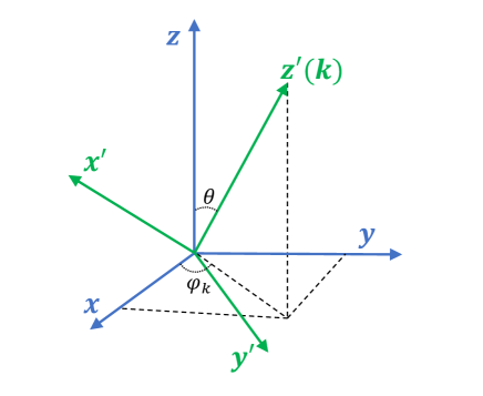
Figure 7: Relation between the wave-vector-dependent coordinate frame (the green arrows) and the fixed lab coordinate (the blue arrows).

For convenience, we define the following amplitude function

$$\psi_{\lambda}(\bm{r},t)=\frac{1}{\sqrt{(2\pi)^{3}}}\int d^{3}k\xi_{\lambda}(\bm{k})e^{i[(\bm{k}\cdot\bm{r}-\omega)t+\lambda\varphi_{k}]},$$ (180)

which is the effective wave function of the photon pulse in real space. For a Bessel pulse, we have

$$\psi_{\lambda}(\bm{r},t)= \sqrt{\frac{k_{\perp,c}}{2\pi\sigma_{z}\sigma_{\rho}}}i^{m+\lambda}J_{m+\lambda}(k_{\perp,c}\rho)e^{i(m+\lambda)\varphi}\exp\left[-\frac{\left(ct-z\cos\theta_{c}\right)^{2}}{4\sigma_{z}^{2}\cos^{2}\theta_{c}}-ik_{z,c}(z-t/\cos\theta_{c})\right]$$ (181)

$$= \sqrt{\frac{C_{0}}{2\pi V_{p}}}i^{m+\lambda}J_{m+\lambda}(k_{\perp,c}\rho)e^{i(m+\lambda)\varphi}\exp\left[-\frac{\left(ct-z\cos\theta_{c}\right)^{2}}{4\sigma_{z}^{2}\cos^{2}\theta_{c}}-ik_{z,c}(z-t/\cos\theta_{c})\right],$$ (182)

where the constant $C_{0}=k_{z,c}\sigma_{z}=k_{\perp,c}\sigma_{\rho}\gg 1$ describes the sharpness of the SAF, $V_{p}=\sigma_{z}\sigma_{\rho}^{2}$ characterizes the effective volume of the photon pulse, and we have used the Jacobi-Anger expansion

$$e^{iz\cos\theta} =\sum_{n=-\infty}^{\infty}i^{n}J_{n}(z)e^{in\theta},$$ (183)

$$e^{-iz\cos\theta} =e^{iz\cos(\theta+\pi)}=\sum_{n=-\infty}^{\infty}i^{n}J_{n}(z)e^{in(\theta+\pi)}=\sum_{n=-\infty}^{\infty}(-i)^{n}J_{n}(z)e^{in\theta},$$ (184)

with the $n$th Bessel function of the first kind

$$J_{n}(z)=\frac{1}{2\pi}\int_{0}^{2\pi}e^{i(n\varphi-z\sin\varphi)}d\varphi.$$ (185)

Then, we have

$$\left\langle n_{\xi\lambda}\right|\hat{\bm{s}}^{\rm obs}\left|n_{\xi\lambda}\right\rangle=s_{\lambda}\bm{e}_{\lambda}+s_{-\lambda}\bm{e}_{-\lambda}+\lambda s_{z}\bm{e}_{z}$$ (186)

where $s_{-\lambda}=s_{\lambda}^{*}$,

$$s_{\lambda}= -in\hbar\times\frac{i\lambda}{\sqrt{2}}\sin\theta_{c}\left[\cos^{2}\frac{\theta_{c}}{2}\psi_{0}^{*}(\bm{r},t)\psi_{-\lambda}(\bm{r},t)+\sin^{2}\frac{\theta_{c}}{2}\psi_{\lambda}^{*}(\bm{r},t)\psi_{0}(\bm{r},t)\right]$$ (187)

$$= -\frac{in\hbar C_{0}\sin\theta_{c}}{2\sqrt{2}\pi\sigma_{z}\sigma_{\rho}^{2}}e^{-i\lambda\varphi}\left[\cos^{2}\frac{\theta_{c}}{2}J_{m}(k_{\perp,c}\rho)J_{m-\lambda}(k_{\perp,c}\rho)+\sin^{2}\frac{\theta_{c}}{2}J_{m+\lambda}(k_{\perp,c}\rho)J_{m}(k_{\perp,c}\rho)\right]\exp\left[-\frac{\left(ct-z\cos\theta_{c}\right)^{2}}{2\sigma_{z}^{2}\cos^{2}\theta_{c}}\right],$$ (188)

and

$$s_{z} =-in\hbar\times i\left[\left|\psi_{-\lambda}(\bm{r},t)\right|^{2}\cos^{4}\frac{\theta_{c}}{2}-\left|\psi_{\lambda}(\bm{r},t)\right|\sin^{4}\frac{\theta_{c}}{2}\right]$$ (189)

$$=\frac{n\hbar C_{0}}{2\pi\sigma_{z}\sigma_{\rho}^{2}}\left\{\left[J_{m-\lambda}(k_{\perp,c}\rho)\right]^{2}\cos^{4}\frac{\theta_{c}}{2}-\left[J_{m+\lambda}(k_{\perp,c}\rho)\right]^{2}\sin^{4}\frac{\theta_{c}}{2}\right\}\exp\left[-\frac{\left(ct-z\cos\theta_{c}\right)^{2}}{2\sigma_{z}^{2}\cos^{2}\theta_{c}}\right].$$ (190)

Using the relation $\bm{e}_{\pm\lambda}=(\bm{e}_{x}\pm i\lambda\bm{e}_{y})/\sqrt{2}$, we can express the spin density vector as

$$\left\langle n_{\xi\lambda}\right|\hat{\bm{s}}^{\rm obs}(\bm{r},t)\left|n_{\xi\lambda}\right\rangle =-s_{\varphi}\bm{e}_{x}\sin\lambda\varphi+\lambda s_{\varphi}\bm{e}_{y}\cos\lambda\varphi+\lambda s_{z}\bm{e}_{z}=\lambda\left(s_{\varphi}\bm{e}_{\varphi}+s_{z}\bm{e}_{z}\right),$$ (191)

where

$$s_{\varphi} =\frac{n\hbar C_{0}\sin\theta_{c}}{2\pi\sigma_{z}\sigma_{\rho}^{2}}\left[\cos^{2}\frac{\theta_{c}}{2}J_{m}(k_{\perp,c}\rho)J_{m-\lambda}(k_{\perp,c}\rho)+\sin^{2}\frac{\theta_{c}}{2}J_{m+\lambda}(k_{\perp,c}\rho)J_{m}(k_{\perp,c}\rho)\right]\exp\left[-\frac{\left(ct-z\cos\theta_{c}\right)^{2}}{2\sigma_{z}^{2}\cos^{2}\theta_{c}}\right]$$ (192)

The spin density of a coherent-state Bessel pulse can be evaluated similarly.

VI Quantum correlation of spin density

In this section, we show how to evaluate the quantum correlations of the photon spin density. Due to the vector nature of the spin density, the full two-point correlation should be characterized by a $3\times 3$ correlation matrix

$$G(\bm{r},t;\bm{r}^{\prime},t^{\prime})=\left[\begin{array}[]{ccc}\left\langle\hat{s}_{x}^{{\rm obs}}(\bm{r},t)\hat{s}_{x}^{{\rm obs}}(\bm{r}^{\prime},t^{\prime})\right\rangle&\left\langle\hat{s}_{x}^{{\rm obs}}(\bm{r},t)\hat{s}_{y}^{{\rm obs}}(\bm{r}^{\prime},t^{\prime})\right\rangle&\left\langle\hat{s}_{x}^{{\rm obs}}(\bm{r},t)\hat{s}_{z}^{{\rm obs}}(\bm{r}^{\prime},t^{\prime})\right\rangle\\ \left\langle\hat{s}_{y}^{{\rm obs}}(\bm{r},t)\hat{s}_{x}^{{\rm obs}}(\bm{r}^{\prime},t^{\prime})\right\rangle&\left\langle\hat{s}_{y}^{{\rm obs}}(\bm{r},t)\hat{s}_{y}^{{\rm obs}}(\bm{r}^{\prime},t^{\prime})\right\rangle&\left\langle\hat{s}_{y}^{{\rm obs}}(\bm{r},t)\hat{s}_{z}^{{\rm obs}}(\bm{r}^{\prime},t^{\prime})\right\rangle\\ \left\langle\hat{s}_{z}^{{\rm obs}}(\bm{r},t)\hat{s}_{x}^{{\rm obs}}(\bm{r}^{\prime},t^{\prime})\right\rangle&\left\langle\hat{s}_{z}^{{\rm obs}}(\bm{r},t)\hat{s}_{y}^{{\rm obs}}(\bm{r}^{\prime},t^{\prime})\right\rangle&\left\langle\hat{s}_{z}^{{\rm obs}}(\bm{r},t)\hat{s}_{z}^{{\rm obs}}(\bm{r}^{\prime},t^{\prime})\right\rangle\end{array}\right].$$ (193)

Here, we only concern the equal-time correlator $\left\langle\hat{s}^{\rm obs}_{z}(\bm{r},t)\hat{s}^{\rm obs}_{z}(\bm{r}^{\prime},t)\right\rangle$. To simplify the calculation, we take the paraxial approximation, i.e., $\theta_{c}\approx 0$. Then, the two-point spin-density correlations for a Fock-state and coherent-state pulse are given by

$$\left\langle n_{\xi\lambda}\right|\hat{s}^{\rm obs}_{z}(\bm{r},t)\hat{s}^{\rm obs}_{z}(\bm{r}^{\prime},t)\left|n_{\xi\lambda}\right\rangle\approx \frac{\hbar^{2}}{(2\pi)^{6}}\int d^{3}k_{1}\int d^{3}k_{2}\int d^{3}k_{3}\int d^{3}k_{4}e^{-i[(\bm{k}_{1}-\bm{k}_{2})\cdot\bm{r}+(\bm{k}_{3}-\bm{k}_{4})\cdot\bm{r}^{\prime}-(\omega_{1}-\omega_{2}+\omega_{3}-\omega_{4})t]}e^{i\lambda(\varphi_{k_{1}}-\varphi_{k_{2}}+\varphi_{k_{3}}-\varphi_{k_{4}})}$$

$$\times\left\langle n_{\xi\lambda}\right|\hat{a}_{\bm{k}_{1},\lambda}^{\dagger}\hat{a}_{\bm{k}_{3},\lambda}^{\dagger}\hat{a}_{\bm{k}_{2},\lambda}\hat{a}_{\bm{k}_{4},\lambda}+\delta(\bm{k}_{2}-\bm{k}_{3})\hat{a}_{\bm{k}_{1},\lambda}^{\dagger}\hat{a}_{\bm{k}_{4},\lambda}\left|n_{\xi\lambda}\right\rangle$$ (194)

$$= \hbar^{2}\left[n(n-1)\left|\psi_{-\lambda}(\bm{r},t)\right|^{2}\left|\psi_{-\lambda}(\bm{r}^{\prime},t)\right|^{2}+\delta(\bm{r}-\bm{r}^{\prime})n\left|\psi_{-\lambda}(\bm{r},t)\right|^{2}\right],$$ (195)

and

$$\left\langle\alpha_{\xi\lambda}\right|\hat{s}^{\rm obs}_{z}(\bm{r},t)\hat{s}^{\rm obs}_{z}(\bm{r}^{\prime},t)\left|\alpha_{\xi\lambda}\right\rangle\approx \frac{\hbar^{2}}{(2\pi)^{6}}\int d^{3}k_{1}\int d^{3}k_{2}\int d^{3}k_{3}\int d^{3}k_{4}e^{-i[(\bm{k}_{1}-\bm{k}_{2})\cdot\bm{r}+(\bm{k}_{3}-\bm{k}_{4})\cdot\bm{r}^{\prime}-(\omega_{1}-\omega_{2}+\omega_{3}-\omega_{4})t]}e^{i\lambda(\varphi_{k_{1}}-\varphi_{k_{2}}+\varphi_{k_{3}}-\varphi_{k_{4}})}$$

$$\times\left\langle\alpha_{\xi\lambda}\right|\hat{a}_{\bm{k}_{1},\lambda}^{\dagger}\hat{a}_{\bm{k}_{3},\lambda}^{\dagger}\hat{a}_{\bm{k}_{2},\lambda}\hat{a}_{\bm{k}_{4},\lambda}+\delta(\bm{k}_{2}-\bm{k}_{3})\hat{a}_{\bm{k}_{1},\lambda}^{\dagger}\hat{a}_{\bm{k}_{4},\lambda}\left|\alpha_{\xi\lambda}\right\rangle$$ (196)

$$= \hbar^{2}\left[\bar{n}^{2}\left|\psi_{-\lambda}(\bm{r},t)\right|^{2}\left|\psi_{-\lambda}(\bm{r}^{\prime},t)\right|^{2}+\delta(\bm{r}-\bm{r}^{\prime})\bar{n}\left|\psi_{-\lambda}(\bm{r},t)\right|^{2}\right]$$ (197)

Here, we see that the Poisson and sub-Poisson statistics automatically enter the quantum spin-density correlations.

We note that the delta function $\delta(\bm{r}-\bm{r}^{\prime})$ in the correlator will not lead to any diverging effect, because a practical probe always measures the averaged photon spin density over a finite volume instead of the true single-point spin density. Now we consider the effective volume of the detector is $V_{d}\ll\lambda_{c}^{3}$. For a Fock-state Bessel pulse, the averaged photon spin density detected by this probe is given by

$$\left\langle n_{\xi\lambda}\right|\frac{1}{V_{d}}\int_{V_{d}}d^{3}r\hat{s}^{\rm obs}_{z}(\bm{r},t)\left|n_{\xi\lambda}\right\rangle\approx n\hbar\left|\psi_{-\lambda}(\bm{r},t)\right|^{2}.$$ (198)

The corresponding spin correlation is given by

$$\left\langle n_{\xi\lambda}\right|\frac{1}{V_{d}^{2}}\int d^{3}r\hat{s}^{\rm obs}_{z}(\bm{r},t)\int d^{3}r^{\prime}\hat{s}^{\rm obs}_{z}(\bm{r}^{\prime},t)\left|n_{\xi\lambda}\right\rangle\approx \begin{cases}\hbar^{2}n(n-1)\left|\psi_{-\lambda}(\bm{r},t)\right|^{2}\left|\psi_{-\lambda}(\bm{r}^{\prime},t)\right|^{2},&{\rm for}\ \bm{r}\neq\bm{r}^{\prime}\\ \hbar^{2}n(n-1)\left|\psi_{-\lambda}(\bm{r},t)\right|^{4}+\frac{n\hbar^{2}}{V_{d}}\left|\psi_{-\lambda}(\bm{r},t)\right|^{2},&{\rm for}\ \bm{r}=\bm{r}^{\prime}\end{cases}$$

Then, the uncertainty of the spin density in $z$-direction is given by

$$\Delta\hat{s}^{\rm obs}_{z}\approx\hbar\sqrt{n}\sqrt{\frac{1}{V_{d}}\left|\psi_{-\lambda}(\bm{r},t)\right|^{2}-\left|\psi_{-\lambda}(\bm{r},t)\right|^{4}}.$$ (199)

Usually, the second term will be very small, i.e., the ratio of these two terms can be approximated as $\sqrt{V_{p}/V_{d}}\gg\sqrt{\lambda^{3}_{c}/V_{d}}\gg 1$.

Similarly for a coherent-state pulse, wee have

$$\left\langle\alpha_{\xi\lambda}\right|\frac{1}{V_{d}}\int_{V_{d}}d^{3}r\hat{s}^{\rm obs}_{z}(\bm{r},t)\left|\alpha_{\xi\lambda}\right\rangle\approx\bar{n}\hbar\left|\psi_{-\lambda}(\bm{r},t)\right|^{2}.$$ (200)

The corresponding spin correlation is given by

$$\left\langle\alpha_{\xi\lambda}\right|\frac{1}{V_{d}^{2}}\int d^{3}r\hat{s}^{\rm obs}_{z}(\bm{r},t)\int d^{3}r^{\prime}\hat{s}^{\rm obs}_{z}(\bm{r}^{\prime},t)\left|\alpha_{\xi\lambda}\right\rangle\approx \begin{cases}\hbar^{2}\bar{n}^{2}\left|\psi_{-\lambda}(\bm{r},t)\right|^{2}\left|\psi_{-\lambda}(\bm{r}^{\prime},t)\right|^{2},&{\rm for}\ \bm{r}\neq\bm{r}^{\prime}\\ \hbar^{2}\bar{n}^{2}\left|\psi_{-\lambda}(\bm{r},t)\right|^{4}+\frac{\bar{n}\hbar^{2}}{V_{d}}\left|\psi_{-\lambda}(\bm{r},t)\right|^{2},&{\rm for}\ \bm{r}=\bm{r}^{\prime}\end{cases}$$

Then, the corresponding uncertainty of the spin density in $z$-direction is given by

$$\Delta\hat{s}^{\rm obs}_{z}\approx\hbar\sqrt{\frac{\bar{n}}{V_{d}}}\left|\psi_{-\lambda}(\bm{r},t)\right|.$$ (201)