Consistent Sparse Deep Learning: Theory and Computation

Abstract

Deep learning has been the engine powering many successes of data science. However, the deep neural network (DNN), as the basic model of deep learning, is often excessively over-parameterized, causing many difficulties in training, prediction and interpretation. We propose a frequentist-like method for learning sparse DNNs and justify its consistency under the Bayesian framework: the proposed method could learn a sparse DNN with at most $O(n/\log(n))$ connections and nice theoretical guarantees such as posterior consistency, variable selection consistency and asymptotically optimal generalization bounds. In particular, we establish posterior consistency for the sparse DNN with a mixture Gaussian prior, show that the structure of the sparse DNN can be consistently determined using a Laplace approximation-based marginal posterior inclusion probability approach, and use Bayesian evidence to elicit sparse DNNs learned by an optimization method such as stochastic gradient descent in multiple runs with different initializations. The proposed method is computationally more efficient than standard Bayesian methods for large-scale sparse DNNs. The numerical results indicate that the proposed method can perform very well for large-scale network compression and high-dimensional nonlinear variable selection, both advancing interpretable machine learning.

Keywords: Bayesian Evidence; Laplace Approximation; Network Compression; Nonlinear Feature Selection; Posterior Consistency.

1 Introduction

During the past decade, the deep neural network (DNN) has achieved great successes in solving many complex machine learning tasks such as pattern recognition and natural language processing. A key factor to the successes is its superior approximation power over the shallow one (Montufar et al., 2014; Telgarsky, 2017; Yarotsky, 2017; Mhaskar et al., 2017). The DNNs used in practice may consist of hundreds of layers and millions of parameters, see e.g. He et al. (2016) on image classification. Training and operation of DNNs of this scale entail formidable computational challenges. Moreover, the DNN models with massive parameters are more easily overfitted when the training samples are insufficient. DNNs are known to have many redundant parameters (Glorot et al., 2011; Yoon and Hwang, 2017; Scardapane et al., 2017; Denil et al., 2013; Cheng et al., 2015; Mocanu et al., 2018). For example, Denil et al. (2013) showed that in some networks, only 5% of the parameters are enough to achieve acceptable models; and Glorot et al. (2011) showed that sparsity (via employing a ReLU activation function) can generally improve the training and prediction performance of the DNN. Over-parameterization often makes the DNN model less interpretable and miscalibrated (Guo et al., 2017), which can cause serious issues in human-machine trust and thus hinder applications of artificial intelligence (AI) in human life.

The desire to reduce the complexity of DNNs naturally leads to two questions: (i) Is a sparsely connected DNN, also known as sparse DNN, able to approximate the target mapping with a desired accuracy? and (ii) how to train and determine the structure of a sparse DNN? This paper answers these two questions in a coherent way. The proposed method is essentially a regularization method, but justified under the Bayesian framework.

The approximation power of sparse DNNs has been studied in the literature from both frequentist and Bayesian perspectives. From the frequentist perspective, Bölcskei et al. (2019) quantifies the minimum network connectivity that guarantees uniform approximation rates for a class of affine functions; and Schmidt-Hieber (2017) and Bauler and Kohler (2019) characterize the approximation error of a sparsely connected neural network for Hölder smooth functions. From the Bayesian perspective, Liang et al. (2018) established posterior consistency for Bayesian shallow neural networks under mild conditions; and Polson and Ročková (2018) established posterior consistency for Bayesian DNNs but under some restrictive conditions such as a spike-and-slab prior is used for connection weights, the activation function is ReLU, and the number of input variables keeps at an order of $O(1)$ while the sample size grows to infinity.

The existing methods for learning sparse DNNs are usually developed separately from the approximation theory. For example, Alvarez and Salzmann (2016), Scardapane et al. (2017) and Ma et al. (2019) developed some regularization methods for learning sparse DNNs; Wager et al. (2013) showed that dropout training is approximately equivalent to an $L_{2}$-regularization; Han et al. (2015a) introduced a deep compression pipeline, where pruning, trained quantization and Huffman coding work together to reduce the storage requirement of DNNs; Liu et al. (2015) proposed a sparse decomposition method to sparsify convolutional neural networks (CNNs); Frankle and Carbin (2018) considered a lottery ticket hypothesis for selecting a sparse subnetwork; and Ghosh and Doshi-Velez (2017) proposed to learn Bayesian sparse neural networks via node selection with a horseshoe prior under the framework of variational inference. For these methods, it is generally unclear if the resulting sparse DNN is able to provide a desired approximation accuracy to the true mapping and how close in structure the sparse DNN is to the underlying true DNN.

On the other hand, there are some work which developed the approximation theory for sparse DNNs but not the associated learning algorithms, see e.g., Bölcskei et al. (2019) and Polson and Ročková (2018). An exception is Liang et al. (2018), where the population stochastic approximation Monte Carlo (pop-SAMC) algorithm (Song et al., 2014) was employed to learn sparse neural networks. However, since the pop-SAMC algorithm belongs to the class of traditional MCMC algorithms, where the full data likelihood needs to be evaluated at each iteration, it is not scalable for big data problems. Moreover, it needs to run for a large number of iterations for ensuring convergence. As an alternative to overcome the convergence issue of MCMC simulations, the variational Bayesian method (Jordan et al., 1999) has been widely used in the machine learning community. Recently, it has been applied to learn Bayesian neural networks (BNNs), see e.g., Mnih and Gregor (2014) and Blundell et al. (2015). However, theoretical properties of the variational posterior of the BNN are still not well understood due to its approximation nature.

This paper provides a frequentist-like method for learning sparse DNNs, which, with theoretical guarantee, converges to the underlying true DNN model in probability. The proposed method is to first train a dense DNN using an optimization method such as stochastic gradient descent (SGD) by maximizing its posterior distribution with a mixture Gaussian prior, and then sparsify its structure according to the Laplace approximation of the marginal posterior inclusion probabilities. Finally, Bayesian evidence is used as the criterion for eliciting sparse DNNs learned by the optimization method in multiple runs with different initializations. To justify consistency of the sparsified DNN, we first establish posterior consistency for Bayesian DNNs with mixture Gaussian priors and consistency of structure selection for Bayesian DNNs based on the marginal posterior inclusion probabilities, and then establish consistency of the sparsified DNN via Laplace approximation to the marginal posterior inclusion probabilities. In addition, we show that the Bayesian sparse DNN has asymptotically an optimal generalization bound.

The proposed method works with various activation functions such as sigmoid, tanh and ReLU, and our theory allows the number of input variables to increase with the training sample size in an exponential rate. Under regularity conditions, the proposed method learns a sparse DNN of size $O(n/\log(n))$ with nice theoretical guarantees such as posterior consistency, variable selection consistency, and asymptotically optimal generalization bound. Since, for the proposed method, the DNN only needs to be trained using an optimization method, it is computationally much more efficient than standard Bayesian methods. As a by-product, this work also provides an effective method for high-dimensional nonlinear variable selection. Our numerical results indicate that the proposed method can work very well for large-scale DNN compression and high-dimensional nonlinear variable selection. For some benchmark DNN compression examples, the proposed method produced the state-of-the-art prediction accuracy using about the same amounts of parameters as the existing methods. In summary, this paper provides a complete treatment for sparse DNNs in both theory and computation.

The remaining part of the paper is organized as follows. Section 2 studies the consistency theory of Bayesian sparse DNNs. Section 3 proposes a computational method for training sparse DNNs. Section 4 presents some numerical examples. Section 5 concludes the paper with a brief discussion.

2 Consistent Sparse DNNs: Theory

2.1 Bayesian Sparse DNNs with mixture Gaussian Prior

Let $D_{n}=(\boldsymbol{x}^{(i)},y^{(i)})_{i=1,...,n}$ denote a training dataset of $n$ $i.i.d$ observations, where $\boldsymbol{x}^{(i)}\in R^{p_{n}}$, $y^{(i)}\in R$, and $p_{n}$ denotes the dimension of input variables and is assumed to grow with the training sample size $n$. We first study the posterior approximation theory of Bayesian sparse DNNs under the framework of generalized linear models, for which the distribution of $y$ given ${\boldsymbol{x}}$ is given by

$$f(y|\mu^{*}({\boldsymbol{x}}))=\exp\{A(\mu^{*}({\boldsymbol{x}}))y+B(\mu^{*}({\boldsymbol{x}}))+C(y)\},$$

where $\mu^{*}({\boldsymbol{x}})$ denotes a nonlinear function of ${\boldsymbol{x}}$, and $A(\cdot)$, $B(\cdot)$ and $C(\cdot)$ are appropriately defined functions. The theoretical results presented in this work mainly focus on logistic regression models and normal linear regression models. For logistic regression, we have $A(\mu^{*})=\mu^{*}$, $B(\mu^{*})=-\log(1+e^{\mu^{*}})$, and $C(y)=1$. For normal regression, by introducing an extra dispersion parameter $\sigma^{2}$, we have $A(\mu^{*})=\mu^{*}/\sigma^{2}$, $B(\mu^{*})=-{\mu^{*}}^{2}/2\sigma^{2}$ and $C(y)=-y^{2}/2\sigma^{2}-\log(2\pi\sigma^{2})/2$. For simplicity, $\sigma^{2}=1$ is assumed to be known in this paper. How to extend our results to the case that $\sigma^{2}$ is unknown will be discussed in Remark 2.3.

We approximate $\mu^{*}({\boldsymbol{x}})$ using a DNN. Consider a DNN with $H_{n}-1$ hidden layers and $L_{h}$ hidden units at layer $h$, where $L_{H_{n}}=1$ for the output layer and $L_{0}=p_{n}$ for the input layer. Let $\boldsymbol{w}^{h}\in\mathbb{R}^{L_{h}\times L_{h-1}}$ and $\boldsymbol{b}^{h}\in\mathbb{R}^{L_{h}\times 1}$, $h\in\{1,2,...,H_{n}\}$ denote the weights and bias of layer $h$, and let $\psi^{h}:R^{L_{h}\times 1}\to\mathbb{R}^{L_{h}\times 1}$ denote a coordinate-wise and piecewise differentiable activation function of layer $h$. The DNN forms a nonlinear mapping

$$\mu({\boldsymbol{\beta}},\boldsymbol{x})=\boldsymbol{w}^{H_{n}}\psi^{H_{n}-1}\left[\cdots\psi^{1}\left[\boldsymbol{w}^{1}\boldsymbol{x}+\boldsymbol{b}^{1}\right]\cdots\right]+\boldsymbol{b}^{H_{n}},$$ (1)

where ${\boldsymbol{\beta}}=({\boldsymbol{w}},{\boldsymbol{b}})=\left\{{w}_{ij}^{h},{b}_{k}^{h}:h\in\{1,2,...,H_{n}\},i,k\in\{1,...,L_{h}\},j\in\{1,...,L_{h-1}\}\right\}$ denotes the collection of all weights and biases, consisting of $K_{n}=\sum_{h=1}^{H_{n}}\left(L_{h-1}\times L_{h}+L_{h}\right)$ elements in total. To facilitate representation of the sparse DNN, we introduce an indicator variable for each weight and bias of the DNN, which indicates the existence of the connection in the network. Let ${\boldsymbol{\gamma}}^{\boldsymbol{w}^{h}}$ and ${\boldsymbol{\gamma}}^{\boldsymbol{b}^{h}}$ denote the matrix and vector of the indicator variables associated with $\boldsymbol{w}^{h}$ and $\boldsymbol{b}^{h}$, respectively. Further, we let $\boldsymbol{\gamma}=\{{\boldsymbol{\gamma}}_{ij}^{\boldsymbol{w}^{h}},{\boldsymbol{\gamma}}_{k}^{\boldsymbol{b}^{h}}:h\in\{1,2,...,H_{n}\}$, $i,k\in\left\{1,...,L_{h}\right\},j\in\left\{1,...,L_{h-1}\right\}\}$ and $\boldsymbol{\beta}_{\boldsymbol{\gamma}}=\{{w}_{ij}^{h},{b}_{k}^{h}:{\boldsymbol{\gamma}}_{ij}^{\boldsymbol{w}^{h}}=1,{\boldsymbol{\gamma}}_{k}^{\boldsymbol{b}^{h}}=1$ ,$h\in\{1,2,...,H_{n}\},i,k\in\left\{1,...,L_{h}\right\}$, $j\in\left\{1,...,L_{h-1}\right\}\}$, which specify, respectively, the structure and associated parameters for a sparse DNN.

To conduct Bayesian analysis for the sparse DNN, we consider a mixture Gaussian prior specified as follows:

$${\boldsymbol{\gamma}}_{ij}^{\boldsymbol{w}^{h}}\sim Bernoulli(\lambda_{n}),\quad{\boldsymbol{\gamma}}_{k}^{\boldsymbol{b}^{h}}\sim Bernoulli(\lambda_{n}),$$ (2)

$${{\boldsymbol{w}}}_{ij}^{h}|{\boldsymbol{\gamma}}_{ij}^{\boldsymbol{w}^{h}}\sim{\boldsymbol{\gamma}}_{ij}^{\boldsymbol{w}^{h}}N(0,\sigma_{1,n}^{2})+(1-{\boldsymbol{\gamma}}_{ij}^{\boldsymbol{w}^{h}})N(0,\sigma_{0,n}^{2}),\ \ {{\boldsymbol{b}}}_{k}^{h}|{\boldsymbol{\gamma}}_{k}^{\boldsymbol{b}^{h}}\sim{\boldsymbol{\gamma}}_{k}^{\boldsymbol{b}^{h}}N(0,\sigma_{1,n}^{2})+(1-{\boldsymbol{\gamma}}_{k}^{\boldsymbol{b}^{h}})N(0,\sigma_{0,n}^{2}),$$ (3)

where $h\in\{1,2,...,H_{N}\},i\in\left\{1,...,L_{h-1}\right\},j,k\in\left\{1,...,L_{h}\right\}$, and $\sigma_{0,n}^{2}<\sigma_{1,n}^{2}$ are prespecified constants. Marginally, we have

$${w}_{ij}^{h}\sim\lambda_{n}N(0,\sigma_{1,n}^{2})+(1-\lambda_{n})N(0,\sigma_{0,n}^{2}),\ \ {b}_{k}^{h}\sim\lambda_{n}N(0,\sigma_{1,n}^{2})+(1-\lambda_{n})N(0,\sigma_{0,n}^{2}).\\$$ (4)

Typically, we set $\sigma_{0,n}^{2}$ to be a very small value while $\sigma_{1,n}^{2}$ to be relatively large. When $\sigma_{0,n}^{2}\rightarrow 0$, the prior is reduced to the spike-and-slab prior (Ishwaran et al., 2005). Therefore, this prior can be viewed as a continuous relaxation of the spike-and-slab prior. Such a prior has been used by many authors in Bayesian variable selection, see e.g., George and McCulloch (1993) and Song and Liang (2017).

2.2 Posterior Consistency

Posterior consistency plays a major role in validating Bayesian methods especially for high-dimensional models, see e.g. Jiang (2007) and Liang et al. (2013). For DNNs, since the total number of parameters $K_{n}$ is often much larger than the sample size $n$, posterior consistency provides a general guideline in prior setting or choosing prior hyperparameters for a class of prior distributions. Otherwise, the prior information may dominate data information, rendering a biased inference for the underlying true model. In what follows, we prove the posterior consistency of the DNN model with the mixture Gaussian prior (4).

With slight abuse of notation, we rewrite $\mu({\boldsymbol{\beta}},{\boldsymbol{x}})$ in (1) as $\mu({\boldsymbol{\beta}},{\boldsymbol{\gamma}},{\boldsymbol{x}})$ for a sparse network by including its network structure information. We assume $\mu^{*}({\boldsymbol{x}})$ can be well approximated by a sparse DNN with relevant variables, and call this sparse DNN as the true DNN in this paper. More precisely, we define the true DNN as

$$({\boldsymbol{\beta}}^{*},{\boldsymbol{\gamma}}^{*})=\underset{({\boldsymbol{\beta}},{\boldsymbol{\gamma}})\in{\cal G}_{n},\,\|\mu({\boldsymbol{\beta}},{\boldsymbol{\gamma}},{\boldsymbol{x}})-\mu^{*}({\boldsymbol{x}})\|_{L^{2}(\Omega)}\leq\varpi_{n}}{\operatorname{arg\,min}}|{\boldsymbol{\gamma}}|,$$ (5)

where ${\cal G}_{n}:={\cal G}(C_{0},C_{1},\varepsilon,p_{n},H_{n},L_{1},L_{2},\ldots,L_{H_{n}})$ denotes the space of valid sparse networks satisfying condition A.2 (given below) for the given values of $H_{n}$, $p_{n}$, and $L_{h}$’s, and $\varpi_{n}$ is some sequence converging to 0 as $n\to\infty$. For any given DNN $({\boldsymbol{\beta}},{\boldsymbol{\gamma}})$, the error $\mu({\boldsymbol{\beta}},{\boldsymbol{\gamma}},{\boldsymbol{x}})-\mu^{*}({\boldsymbol{x}})$ can be generally decomposed as the network approximation error $\mu({\boldsymbol{\beta}}^{*},{\boldsymbol{\gamma}}^{*},{\boldsymbol{x}})-\mu^{*}({\boldsymbol{x}})$ and the network estimation error $\mu({\boldsymbol{\beta}},{\boldsymbol{\gamma}},{\boldsymbol{x}})-\mu({\boldsymbol{\beta}}^{*},{\boldsymbol{\gamma}}^{*},{\boldsymbol{x}})$. The $L_{2}$ norm of the former one is bounded by $\varpi_{n}$, and the order of the latter will be given in Theorem 2.1. In what follows, we will treat $\varpi_{n}$ as the network approximation error. In addition, we make the following assumptions:

1. The input ${\boldsymbol{x}}$ is bounded by 1 entry-wisely, i.e. ${\boldsymbol{x}}\in\Omega=[-1,1]^{p_{n}}$, and the density of ${\boldsymbol{x}}$ is bounded in its support $\Omega$ uniformly with respect to $n$.

2. The true sparse DNN model satisfies the following conditions:

   • The network structure satisfies: $r_{n}H_{n}\log n$ $+r_{n}\log\overline{L}+s_{n}\log p_{n}\leq C_{0}n^{1-\varepsilon}$, where $0<\varepsilon<1$ is a small constant, $r_{n}=|{\boldsymbol{\gamma}}^{*}|$ denotes the connectivity of ${\boldsymbol{\gamma}}^{*}$, $\overline{L}=\max_{1\leq j\leq H_{n}-1}L_{j}$ denotes the maximum hidden layer width, $s_{n}$ denotes the input dimension of ${\boldsymbol{\gamma}}^{*}$.

   • The network weights are polynomially bounded: $\|{\boldsymbol{\beta}}^{*}\|_{\infty}\leq E_{n}$, where $E_{n}=n^{C_{1}}$ for some constant $C_{1}>0$.

3. The activation function $\psi$ is Lipschitz continuous with a Lipschitz constant of 1.

Assumption A.1 is a typical assumption for posterior consistency, see e.g., Polson and Ročková (2018) and Jiang (2007). In practice, all bounded data can be normalized to satisfy this assumption, e.g. image data are bounded and usually normalized before training. Assumption A.3 is satisfied by many conventional activation functions such as sigmoid, tanh and ReLU.

Assumption A.2 specifies the class of DNN models that we are considering in this paper. They are sparse, while still being able to approximate many types of functions arbitrarily well as the training sample size becomes large, i.e., $\lim_{n\to\infty}\varpi_{n}=0$. The approximation power of sparse DNNs has been studied in several existing work. For example, for the functions that can be represented by an affine system, Bölcskei et al. (2019) proved that if the network parameters are bounded in absolute value by some polynomial $g(r_{n})$, i.e. $||{\boldsymbol{\beta}}^{*}||_{\infty}\leq g(r_{n})$, then the approximation error $\varpi_{n}=O(r_{n}^{-\alpha^{*}})$ for some constant $\alpha^{*}$. To fit this this result into our framework, we can let $r_{n}\asymp n^{(1-\epsilon)/2}$ for some $0<\epsilon<1$, $p_{n}=d$ for some constant $d$, $H_{n}<r_{n}+d$ and $\bar{L}<r_{n}$ (i.e. the setting given in Proposition 3.6 of Bölcskei et al. (2019)). Suppose that the degree of $g(\cdot)$ is $c_{2}$, i.e. $g(r_{n})\prec r_{n}^{c_{2}}$, then $\|{\boldsymbol{\beta}}^{*}\|_{\infty}\prec n^{c_{2}(1-\epsilon)/2}\prec n^{C_{1}}=E_{n}$ for some constant $C_{1}>c_{2}(1-\epsilon)/2$. Therefore, Assumption A.2 is satisfied with the approximation error $\varpi_{n}=O(r_{n}^{-\alpha^{*}})=O(n^{-\alpha^{*}(1-\epsilon)/2})\stackrel{{\scriptstyle\Delta}}{{=}}O(n^{-\varsigma})$ (by defining $\varsigma=\alpha^{*}(1-\epsilon)/2$), which goes to 0 as $n\to\infty$. In summary, the minimax rate in $\sup_{\mu^{*}({\boldsymbol{x}})\in\mathcal{C}}\,\inf_{({\boldsymbol{\beta}},{\boldsymbol{\gamma}})\in\mathcal{G}}\|\mu({\boldsymbol{\beta}},{\boldsymbol{\gamma}},{\boldsymbol{x}})-\mu^{*}({\boldsymbol{x}})\|_{L^{2}(\Omega)}\in\mathcal{O}(n^{-\varsigma})$ can be achieved by sparse DNNs under our assumptions, where $\mathcal{C}$ denotes the class of functions represented by an affine system.

Other than affine functions, our setup for the sparse DNN also matches the approximation theory for many other types of functions. For example, Corollary 3.7 of Petersen and Voigtlaender (2018) showed that for a wide class of piecewise smooth functions with a fixed input dimension, a fixed depth ReLU network can achieve an $\varpi_{n}$-approximation with $\log(r_{n})=O(-\log\varpi_{n})$ and $\log E_{n}=O(-\log\varpi_{n})$. This result satisfies condition A.2 by setting $\varpi_{n}=O(n^{-\varsigma})$ for some constant $\varsigma>0$. As another example, Theorem 3 of Schmidt-Hieber (2017) (see also lemma 5.1 of Polson and Ročková (2018)) proved that any bounded $\alpha$-Hölder smooth function $\mu^{*}({\boldsymbol{x}})$ can be approximated by a sparse ReLU DNN with the network approximation error $\varpi_{n}=O(\log(n)^{\alpha/p_{n}}n^{-\alpha/(2\alpha+p_{n})})$ for some $H_{n}\asymp\log n\log p_{n}$, $L_{j}\asymp p_{n}n^{p_{n}/(2\alpha+p_{n})}/\log n$, $r_{n}=O(p_{n}^{2}\alpha^{2p_{n}}n^{p_{n}/(2\alpha+p_{n})}\log p_{n}$), and $E_{n}=C$ for some fixed constant $C>0$. This result also satisfies condition A.2.2 as long as $p_{n}^{2}\ll\log n$.

It is important to note that there is a fundamental difference between the existing neural network approximation theory and ours. In the existing neural network approximation theory, no data is involved and a small network can potentially achieve an arbitrarily small approximation error by allowing the connection weights to take values in an unbounded space. In contrast, in our theory, the network approximation error, the network size, and the bound of connection weights are all linked to the training sample size. A small network approximation error is required only when the training sample size is large; otherwise, over-fitting might be a concern from the point of view of statistical modeling. In the practice of modern neural networks, the depth and width have been increased without much scruple. These increases reduce the training error, improve the generalization performance under certain regimes (Nakkiran et al., 2020), but negatively affect model calibration (Guo et al., 2017). We expect that our theory can tame the powerful neural networks into the framework of statistical modeling; that is, by selecting an appropriate network size according to the training sample size, the proposed method can generally improve the generalization and calibration of the DNN model while controlling the training error to a reasonable level. The calibration of the sparse DNN will be explored elsewhere.

Let $P^{*}$ and $E^{*}$ denote the respective probability measure and expectation for data $D_{n}$. Let $d(p_{1},p_{2})=\left(\int\left[p_{1}^{\frac{1}{2}}(\boldsymbol{x},y)-p_{2}^{\frac{1}{2}}(\boldsymbol{x},y)\right]^{2}dyd\boldsymbol{x}\right)^{\frac{1}{2}}$ denote the Hellinger distance between two density functions $p_{1}(\boldsymbol{x},y)$ and $p_{2}(\boldsymbol{x},y)$. Let $\pi(A\mid D_{n})$ be the posterior probability of an event $A$. The following theorem establishes posterior consistency for sparse DNNs under the mixture Gaussian prior (4).

Theorem 2.1.

Suppose Assumptions A.1-A.3 hold. If the mixture Gaussian prior (4) satisfies the conditions: $\lambda_{n}=O(1/\{K_{n}[n^{H_{n}}(\overline{L}p_{n})]^{\tau}\})$ for some constant $\tau>0$, $E_{n}/\{H_{n}\log n+\log\overline{L}\}^{1/2}\lesssim\sigma_{1,n}\lesssim n^{\alpha}$ for some constant $\alpha>0$, and $\sigma_{0,n}\lesssim\min\big{\{}1/\{\sqrt{n}K_{n}(n^{3/2}\sigma_{1,0}/H_{n})^{H_{n}}\}$, $1/\{\sqrt{n}K_{n}(nE_{n}/H_{n})^{H_{n}}\}\big{\}}$, then there exists an error sequence $\epsilon_{n}^{2}=O(\varpi_{n}^{2})+O(\zeta_{n}^{2})$ such that $\lim_{n\to\infty}\epsilon_{n}=0$ and $\lim_{n\to\infty}n\epsilon_{n}^{2}=\infty$, and the posterior distribution satisfies

$$\begin{split}&P^{*}\left\{\pi[d(p_{{\boldsymbol{\beta}}},p_{\mu^{*}})>4\epsilon_{n}|D_{n}]\geq 2e^{-cn\epsilon_{n}^{2}}\right\}\leq 2e^{-cn\epsilon_{n}^{2}},\\ &E_{D_{n}}^{*}\pi[d(p_{{\boldsymbol{\beta}}},p_{\mu^{*}})>4\epsilon_{n}|D_{n}]\leq 4e^{-2cn\epsilon_{n}^{2}},\end{split}$$ (6)

for sufficiently large $n$, where $c$ denotes a constant, $\zeta_{n}^{2}=[r_{n}H_{n}\log n+r_{n}\log\overline{L}+s_{n}\log p_{n}]/n$, $p_{\mu^{*}}$ denotes the underlying true data distribution, and $p_{\boldsymbol{\beta}}$ denotes the data distribution reconstructed by the Bayesian DNN based on its posterior samples.

The proof of Theorem 2.1 can be found in the supplementary material. Regarding this theorem, we have a few remarks:

Remark 2.1.

Theorem 2.1 provides a posterior contraction rate $\epsilon_{n}$ for the sparse BNN. The contraction rate contains two components, $\varpi_{n}$ and $\zeta_{n}$, where $\varpi_{n}$, as defined previously, represents the network approximation error, and $\zeta_{n}$ represents the network estimation error measured in Hellinger distance. Since the estimation error $\zeta_{n}$ grows with the network connectivity $r_{n}$, there is a trade-off between the network approximation error and the network estimation error. A larger network has a lower approximation error and a higher estimation error, and vice versa.

Remark 2.2.

Theorem 2.1 implies that given a training sample size $n$, the proposed method can learn a sparse neural network with at most $O(n/\log(n))$ connections. Compared to the fully connected DNN, the sparsity of the proposed BNN enables some theoretical guarantees for its performance. The sparse BNN has nice theoretical properties, such as posterior consistency, variable selection consistency, and asymptotically optimal generalization bounds, which are beyond the ability of general neural networks. The latter two properties will be established in Section 2.3 and Section 2.4, respectively.

Remark 2.3.

Although Theorem 2.1 is proved by assuming $\sigma^{2}$ is known, it can be easily extended to the case that $\sigma^{2}$ is unknown by assuming an inverse gamma prior $\sigma^{2}\sim\mbox{IG}(a_{0},b_{0})$ for some constants $a_{0},b_{0}>0$. If a relatively uninformative prior is desired, one can choose $a_{0}\in(0,1)$ such that the inverse gamma prior is very diffuse with a non-existing mean value. However, if $a_{0}=b_{0}=0$, i.e., the Jeffreys prior $\pi(\sigma^{2})\propto 1/\sigma^{2}$, the posterior consistency theory established Theorem 2.1 might not hold any more. In general, to achieve posterior consistency, the prior is required, at least in the framework adopted by the paper, to satisfy two conditions (Ghosal et al., 2000; Jiang, 2007): (i) a not too little prior probability is placed over the neighborhood of the true density, and (ii) a very little prior probability is placed outside of a region that is not too complex. Obviously, the Jeffreys prior and thus the joint prior of $\sigma^{2}$ and the regression coefficients do not satisfy neither of the two conditions. We note that the inverse gamma prior $\sigma^{2}\sim IG(a_{0},b_{0})$ has long been used in Bayesian inference for many different statistical models, such as linear regression (George and McCulloch, 1997), nonparametric regression (Kohn et al., 2001), and Gaussian graphical models (Dobra et al., 2004).

2.3 Consistency of DNN Structure Selection

This section establishes consistency of DNN structure selection under posterior consistency. It is known that the DNN model is generally nonidentifiable due to the symmetry of the network structure. For example, the approximation $\mu({\boldsymbol{\beta}},{\boldsymbol{\gamma}},{\boldsymbol{x}})$ can be invariant if one permutes the orders of certain hidden nodes, simultaneously changes the signs of certain weights and biases if $tanh$ is used as the activation function, or re-scales certain weights and bias if Relu is used as the activation function. However, by introducing appropriate constraints, see e.g., Pourzanjani et al. (2017) and Liang et al. (2018), we can define a set of neural networks such that any possible neural networks can be represented by one and only one neural network in the set via nodes permutation, sign changes, weight rescaling, etc. Let $\Theta$ denote such set of DNNs, where each element in $\Theta$ can be viewed as an equivalent class of DNN models. Let $\nu({\boldsymbol{\gamma}},{\boldsymbol{\beta}})\in\Theta$ be an operator that maps any neural network to $\Theta$ via appropriate transformations such as nodes permutation, sign changes, weight rescaling, etc. To serve the purpose of structure selection in the space $\Theta$, we consider the marginal posterior inclusion probability approach proposed in Liang et al. (2013) for high-dimensional variable selection.

For a better description of this approach, we reparameterize ${\boldsymbol{\beta}}$ and ${\boldsymbol{\gamma}}$ as ${\boldsymbol{\beta}}=({\boldsymbol{\beta}}_{1},{\boldsymbol{\beta}}_{2},\ldots,{\boldsymbol{\beta}}_{K_{n}})$ and ${\boldsymbol{\gamma}}=({\boldsymbol{\gamma}}_{1},{\boldsymbol{\gamma}}_{2},\ldots,{\boldsymbol{\gamma}}_{K_{n}})$, respectively, according to their elements. Without possible confusions, we will often use the indicator vector ${\boldsymbol{\gamma}}$ and the active set $\{i:{\boldsymbol{\gamma}}_{i}=1,i=1,2,\ldots,K_{n}\}$ exchangeably; that is, $i\in{\boldsymbol{\gamma}}$ and ${\boldsymbol{\gamma}}_{i}=1$ are equivalent. In addition, we will treat the connection weights ${\boldsymbol{w}}$ and the hidden unit biases ${\boldsymbol{b}}$ equally; that is, they will not be distinguished in ${\boldsymbol{\beta}}$ and ${\boldsymbol{\gamma}}$. For convenience, we will call each element of ${\boldsymbol{\beta}}$ and ${\boldsymbol{\gamma}}$ a ‘connection’ in what follows.

2.3.1 Marginal Posterior Inclusion Probability Approach

For each connection $c_{i}$, we define its marginal posterior inclusion probability by

$$q_{i}=\int\sum_{{\boldsymbol{\gamma}}}e_{i|\nu({\boldsymbol{\gamma}},{\boldsymbol{\beta}})}\pi({\boldsymbol{\gamma}}|{\boldsymbol{\beta}},D_{n})\pi({\boldsymbol{\beta}}|D_{n})d{\boldsymbol{\beta}},\quad i=1,2,\ldots,K_{n},$$ (7)

where $e_{i|\nu({\boldsymbol{\gamma}},{\boldsymbol{\beta}})}$ is the indicator for the existence of connection $c_{i}$ in the network $\nu({\boldsymbol{\gamma}},{\boldsymbol{\beta}})$. Similarly, we define $e_{i|\nu({\boldsymbol{\gamma}}^{*},{\boldsymbol{\beta}}^{*})}$ as the indicator for the existence of connection $c_{i}$ in the true model $\nu({\boldsymbol{\gamma}}^{*},{\boldsymbol{\beta}}^{*})$. The proposed approach is to choose the connections whose marginal posterior inclusion probabilities are greater than a threshold value $\hat{q}$; that is, setting $\hat{{\boldsymbol{\gamma}}}_{\hat{q}}=\{i:q_{i}>\hat{q},i=1,2,\ldots,K_{n}\}$ as an estimator of ${\boldsymbol{\gamma}}_{*}=\{i:e_{i|\nu({\boldsymbol{\gamma}}^{*},{\boldsymbol{\beta}}^{*})}=1,i=1,\ldots,K_{n}\}$, where ${\boldsymbol{\gamma}}_{*}$ can be viewed as the uniquenized true model. To establish the consistency of $\hat{{\boldsymbol{\gamma}}}_{\hat{q}}$, an identifiability condition for the true model is needed. Let $A(\epsilon_{n})=\{{\boldsymbol{\beta}}:d(p_{\boldsymbol{\beta}},p_{\mu^{*}})\geq\epsilon_{n}\}$. Define

$$\rho(\epsilon_{n})=\max_{1\leq i\leq K_{n}}\int_{A(\epsilon_{n})^{c}}\sum_{{\boldsymbol{\gamma}}}|e_{i|\nu({\boldsymbol{\gamma}},{\boldsymbol{\beta}})}-e_{i|\nu({\boldsymbol{\gamma}}^{*},{\boldsymbol{\beta}}^{*})}|\pi({\boldsymbol{\gamma}}|{\boldsymbol{\beta}},D_{n})\pi({\boldsymbol{\beta}}|D_{n})d{\boldsymbol{\beta}},$$

which measures the structure difference between the true model and the sampled models on the set $A({\epsilon_{n}})^{c}$. Then the identifiability condition can be stated as follows:

1. $\rho(\epsilon_{n})\to 0$, as $n\to\infty$ and $\epsilon_{n}\to 0$.

That is, when $n$ is sufficiently large, if a DNN has approximately the same probability distribution as the true DNN, then the structure of the DNN, after mapping into the parameter space $\Theta$, must coincide with that of the true DNN. Note that this identifiability is different from the one mentioned at the beginning of the section. The earlier one is only with respect to structure and parameter rearrangement of the DNN. Theorem 2.2 concerns consistency of $\hat{{\boldsymbol{\gamma}}}_{\hat{q}}$ and its sure screening property, whose proof is given in the supplementary material.

Theorem 2.2.

Assume that the conditions of Theorem 2.1 and the identifiability condition B.1 hold. Then

• $\max_{1\leq i\leq K_{n}}\{|q_{i}-e_{i|\nu({\boldsymbol{\gamma}}^{*},{\boldsymbol{\beta}}^{*})}|\}\stackrel{{\scriptstyle p}}{{\to}}0$, where $\stackrel{{\scriptstyle p}}{{\to}}$ denotes convergence in probability;

• (sure screening) $P({\boldsymbol{\gamma}}_{*}\subset\hat{{\boldsymbol{\gamma}}}_{\hat{q}})\stackrel{{\scriptstyle p}}{{\to}}1$ for any pre-specified $\hat{q}\in(0,1)$.

• (Consistency) $P({\boldsymbol{\gamma}}_{*}=\hat{{\boldsymbol{\gamma}}}_{0.5})\stackrel{{\scriptstyle p}}{{\to}}1$.

For a network ${\boldsymbol{\gamma}}$, it is easy to identify the relevant variables. Recall that ${\boldsymbol{\gamma}}^{{\boldsymbol{w}}^{h}}\in\mathbb{R}^{L_{h}\times L_{h-1}}$ denotes the connection indicator matrix of layer $h$. Let

$${\boldsymbol{\gamma}}^{{\boldsymbol{x}}}={\boldsymbol{\gamma}}^{{\boldsymbol{w}}^{H_{n}}}{\boldsymbol{\gamma}}^{{\boldsymbol{w}}^{H_{n}-1}}\cdots{\boldsymbol{\gamma}}^{{\boldsymbol{w}}^{1}}\in\mathbb{R}^{1\times p_{n}},$$ (8)

and let ${\boldsymbol{\gamma}}^{{\boldsymbol{x}}}_{i}$ denote the $i$-th element of ${\boldsymbol{\gamma}}^{{\boldsymbol{x}}}$. It is easy to see that if ${\boldsymbol{\gamma}}^{{\boldsymbol{x}}}_{i}>0$ then the variable ${\boldsymbol{x}}_{i}$ is effective in the network ${\boldsymbol{\gamma}}$, and ${\boldsymbol{\gamma}}^{{\boldsymbol{x}}}_{i}=0$ otherwise. Let $e_{{\boldsymbol{x}}_{i}|\nu({\boldsymbol{\gamma}}^{*},{\boldsymbol{\beta}}^{*})}$ be the indicator for the effectiveness of variable ${\boldsymbol{x}}_{i}$ in the network $\nu({\boldsymbol{\gamma}}^{*},{\boldsymbol{\beta}}^{*})$, and let ${\boldsymbol{\gamma}}_{*}^{{\boldsymbol{x}}}=\{i:e_{{\boldsymbol{x}}_{i}|\nu({\boldsymbol{\gamma}}^{*},{\boldsymbol{\beta}}^{*})}=1,i=1,\ldots,p_{n}\}$ denote the set of true variables. Similar to (7), we can define the marginal inclusion probability for each variable:

$$q_{i}^{{\boldsymbol{x}}}=\int\sum_{{\boldsymbol{\gamma}}}e_{{\boldsymbol{x}}_{i}|\nu({\boldsymbol{\gamma}},{\boldsymbol{\beta}})}\pi({\boldsymbol{\gamma}}|{\boldsymbol{\beta}},D_{n})\pi({\boldsymbol{\beta}}|D_{n})d{\boldsymbol{\beta}},\quad i=1,2,\ldots,p_{n},$$ (9)

Then we can select the variables whose marginal posterior inclusion probabilities greater than a threshold $\hat{q}^{{\boldsymbol{x}}}$, e.g., setting $\hat{q}^{{\boldsymbol{x}}}=0.5$. As implied by (8), the consistency of structure selection implies consistency of variable selection.

It is worth noting that the above variable selection consistency result is with respect to the relevant variables defined by the true network ${\boldsymbol{\gamma}}^{*}$. To achieve the variable selection consistency with respect to the relevant variables of $\mu^{*}({\boldsymbol{x}})$, some extra assumptions are needed in defining $({\boldsymbol{\beta}}^{*},{\boldsymbol{\gamma}}^{*})$. How to specify these assumptions is an open problem and we would leave it to readers. However, as shown by our simulation example, the sparse model $({\boldsymbol{\beta}}^{*},{\boldsymbol{\gamma}}^{*})$ defined in (5) works well, which correctly identifies all the relevant variables of the underlying nonlinear system.

2.3.2 Laplace Approximation of Marginal Posterior Inclusion Probabilities

Theorem 2.2 establishes the consistency of DNN structure selection based on the marginal posterior inclusion probabilities. To obtain Bayesian estimates of the marginal posterior inclusion probabilities, intensive Markov Chain Monte Carlo (MCMC) simulations are usually required. Instead of performing MCMC simulations, we propose to approximate the marginal posterior inclusion probabilities using the Laplace method based on the DNN model trained by an optimization method such as SGD. Traditionally, such approximation is required to be performed at the maximum a posteriori (MAP) estimate of the DNN. However, finding the MAP for a large DNN is not computationally guaranteed, as there can be many local minima on its energy landscape. To tackle this issue, we proposed a Bayesian evidence method, see Section 3 for the detail, for eliciting sparse DNN models learned by an optimization method in multiple runs with different initializations. Since conventional optimization methods such as SGD can be used to train the DNN here, the proposed method is computationally much more efficient than the standard Bayesian method. More importantly, as explained in Section 3, consistent estimates of the marginal posterior inclusion probabilities might be obtained at a local maximizer of the log-posterior instead of the MAP estimate. In what follows, we justify the validity of Laplace approximation for marginal posterior inclusion probabilities.

Based on the marginal posterior distribution $\pi({\boldsymbol{\beta}}|D_{n})$, the marginal posterior inclusion probability $q_{i}$ of connection $c_{i}$ can be re-expressed as

$$q_{i}=\int\pi({\boldsymbol{\gamma}}_{i}=1|{\boldsymbol{\beta}})\pi({\boldsymbol{\beta}}|D_{n})d{\boldsymbol{\beta}},\quad i=1,2,\ldots,K_{n}.$$

Under the mixture Gaussian prior, it is easy to derive that

$$\pi({\boldsymbol{\gamma}}_{i}=1|{\boldsymbol{\beta}})=\tilde{b}_{i}/(\tilde{a}_{i}+\tilde{b}_{i}),$$ (10)

where

$$\tilde{a}_{i}=\frac{1-\lambda_{n}}{\sigma_{0,n}}\exp\{-\frac{{\boldsymbol{\beta}}_{i}^{2}}{2\sigma_{0,n}^{2}}\},\quad\tilde{b}_{i}=\frac{\lambda_{n}}{\sigma_{1,n}}\exp\{-\frac{{\boldsymbol{\beta}}_{i}^{2}}{2\sigma_{1,n}^{2}}\}.$$

Let’s define

$$h_{n}({\boldsymbol{\beta}})=\frac{1}{n}\sum_{i=1}^{n}\log(p(y_{i},\boldsymbol{x}_{i}|{\boldsymbol{\beta}}))+\frac{1}{n}\log(\pi({\boldsymbol{\beta}})),$$ (11)

where $p(y_{i},\boldsymbol{x}_{i}|{\boldsymbol{\beta}})$ denotes the likelihood function of the observation $(y_{i},{\boldsymbol{x}}_{i})$ and $\pi({\boldsymbol{\beta}})$ denotes the prior as specified in (4). Then $\pi({\boldsymbol{\beta}}|D_{n})=\frac{e^{nh_{n}({\boldsymbol{\beta}})}}{\int e^{nh_{n}({\boldsymbol{\beta}})}d{\boldsymbol{\beta}}}$ and, for a function $b({\boldsymbol{\beta}})$, the posterior expectation is given by $\frac{\int b({\boldsymbol{\beta}})e^{nh_{n}({\boldsymbol{\beta}})}d{\boldsymbol{\beta}}}{\int e^{nh_{n}({\boldsymbol{\beta}})}d{\boldsymbol{\beta}}}$. Let $\hat{{\boldsymbol{\beta}}}$ denote a strict local maximum of $\pi({\boldsymbol{\beta}}|D_{n})$. Then $\hat{{\boldsymbol{\beta}}}$ is also a local maximum of $h_{n}({\boldsymbol{\beta}})$. Let $B_{\delta}({\boldsymbol{\beta}})$ denote an Euclidean ball of radius $\delta$ centered at ${\boldsymbol{\beta}}$. Let $h_{i_{1},i_{2},\dots,i_{d}}({\boldsymbol{\beta}})$ denote the $d$-th order partial derivative $\frac{\partial^{d}h({\boldsymbol{\beta}})}{\partial{\boldsymbol{\beta}}_{i_{1}}\partial{\boldsymbol{\beta}}_{i_{2}}\cdots\partial{\boldsymbol{\beta}}_{i_{d}}}$, let $H_{n}({\boldsymbol{\beta}})$ denote the Hessian matrix of $h_{n}({\boldsymbol{\beta}})$, let $h_{ij}$ denote the $(i,j)$-th component of the Hessian matrix, and let $h^{ij}$ denote the $(i,j)$-component of the inverse of the Hessian matrix. Recall that ${\boldsymbol{\gamma}}^{*}$ denotes the set of indicators for the connections of the true sparse DNN, $r_{n}$ denotes the size of the true sparse DNN, and $K_{n}$ denotes the size of the fully connected DNN. The following theorem justifies the Laplace approximation of the posterior mean for a bounded function $b({\boldsymbol{\beta}})$.

Theorem 2.3.

Assume that there exist positive numbers $\epsilon$, $M$, $\eta$, and $n_{0}$ such that for any $n>n_{0}$, the function $h_{n}({\boldsymbol{\beta}})$ in (11) satisfies the following conditions:

1. $|h_{i_{1},\dots,i_{d}}(\hat{{\boldsymbol{\beta}}})|<M$ hold for any ${\boldsymbol{\beta}}\in B_{\epsilon}(\hat{{\boldsymbol{\beta}}})$ and any $1\leq i_{1},\dots,i_{d}\leq K_{n}$, where $3\leq d\leq 4$.

2. $|h^{ij}(\hat{{\boldsymbol{\beta}}})|<M$ if ${\boldsymbol{\gamma}}_{i}^{*}={\boldsymbol{\gamma}}_{j}^{*}=1$ and $|h^{ij}(\hat{{\boldsymbol{\beta}}})|=O(\frac{1}{K_{n}^{2}})$ otherwise.

3. $\det(-\frac{n}{2\pi}H_{n}(\hat{{\boldsymbol{\beta}}}))^{\frac{1}{2}}\int_{\mathbb{R}^{K_{n}}\setminus B_{\delta}(\hat{{\boldsymbol{\beta}}})}e^{n(h_{n}({\boldsymbol{\beta}})-h_{n}(\hat{{\boldsymbol{\beta}}}))}d{\boldsymbol{\beta}}=O(\frac{r_{n}^{4}}{n})=o(1)$ for any $0<\delta<\epsilon$.

For any bounded function $b({\boldsymbol{\beta}})$, if $|b_{i_{1},\dots,i_{d}}({\boldsymbol{\beta}})|=|\frac{\partial^{d}b({\boldsymbol{\beta}})}{\partial{\boldsymbol{\beta}}_{i_{1}}\partial{\boldsymbol{\beta}}_{i_{2}}\cdots\partial{\boldsymbol{\beta}}_{i_{d}}}|<M$ holds for any $1\leq d\leq 2$ and any $1\leq i_{1},\dots,i_{d}\leq K_{n}$, then for the posterior mean of $b({\boldsymbol{\beta}})$, we have

$$\frac{\int b({\boldsymbol{\beta}})e^{nh_{n}({\boldsymbol{\beta}})}d{\boldsymbol{\beta}}}{\int e^{nh_{n}({\boldsymbol{\beta}})}d{\boldsymbol{\beta}}}=b(\hat{{\boldsymbol{\beta}}})+O\left(\frac{r_{n}^{4}}{n}\right).$$

Conditions C.1 and C.3 are typical conditions for Laplace approximation, see e.g., Kass et al. (1990). Condition C.2 requires the inverse Hessian to have very small values for the elements corresponding to the false connections. To justify condition C.2, we note that for a multivariate normal distribution, the inverse Hessian is its covariance matrix. Thus, we expect that for the weights with small variance, their corresponding elements in the inverse Hessian matrix would be small as well. The following lemma quantifies the variance of the weights for the false connections.

Lemma 2.1.

Assume that $\sup_{n}\int{|{\boldsymbol{\beta}}_{i}|}^{2+\delta}\pi(\beta_{i}|D_{n})d{\boldsymbol{\beta}}_{i}\leq C<\infty\ a.s.$ for some constants $\delta>0$ and $C>0$ and $\rho(\epsilon_{n})\asymp\pi(d(p_{{\boldsymbol{\beta}}},p_{\mu^{*}})\geq\epsilon_{n}|D_{n})$, where $\rho(\epsilon_{n})$ is defined in Condition B.1. Then with an appropriate choice of prior hyperparameters and $\epsilon_{n}$, $P^{*}\{E({\boldsymbol{\beta}}_{i}^{2}|D_{n})\prec\frac{1}{K_{n}^{2H_{n}-1}}\}\geq 1-2e^{-n\epsilon_{n}^{2}/4}$ holds for any false connection $c_{i}$ in ${\boldsymbol{\gamma}}^{*}$ (i.e., ${\boldsymbol{\gamma}}_{i}^{*}=0$).

In addition, with an appropriate choice of prior hyperparameters, we can also show that $\pi({\boldsymbol{\gamma}}_{i}=1|{\boldsymbol{\beta}})$ satisfies all the requirements of $b({\boldsymbol{\beta}})$ in Theorem 2.3 with a probability tending to 1 as $n\to\infty$ (refer to Section 2.4 of the supplementary material for the detail). Then, by Theorem 2.3, $q_{k}$ and $\pi({\boldsymbol{\gamma}}_{i}=1|\hat{{\boldsymbol{\beta}}})$ are approximately the same as $n\to\infty$, where $\pi({\boldsymbol{\gamma}}_{i}=1|\hat{{\boldsymbol{\beta}}})$ is as defined in (10) but with ${\boldsymbol{\beta}}$ replaced by $\hat{{\boldsymbol{\beta}}}$. Combining with Theorem 2.2, we have that $\pi({\boldsymbol{\gamma}}_{i}=1|\hat{{\boldsymbol{\beta}}})$ is a consistent estimator of $e_{i|\nu({\boldsymbol{\gamma}}^{*},{\boldsymbol{\beta}}^{*})}$.

2.4 Asymptotically Optimal Generalization Bound

This section shows the sparse BNN has asymptotically an optimal generalization bound. First, we introduce a PAC Bayesian bound due to McAllester (1999a, b), where the acronym PAC stands for Probably Approximately Correct. It states that with an arbitrarily high probability, the performance (as provided by a loss function) of a learning algorithm is upper-bounded by a term decaying to an optimal value as more data is collected (hence “approximately correct”). PAC-Bayes has proven over the past two decades to be a powerful tool to derive theoretical guarantees for many machine learning algorithms.

Lemma 2.2 (PAC Bayesian bound).

Let $P$ be any data independent distribution on the machine parameters ${\boldsymbol{\beta}}$, and $Q$ be any distribution that is potentially data-dependent and absolutely continuous with respective to $P$. If the loss function $l({\boldsymbol{\beta}},{\boldsymbol{x}},y)\in[0,1]$, then the following inequality holds with probability $1-\delta$,

$$\int E_{{\boldsymbol{x}},y}l({\boldsymbol{\beta}},{\boldsymbol{x}},y)dQ\leq\int\frac{1}{n}\sum_{i=1}^{n}l({\boldsymbol{\beta}},{\boldsymbol{x}}^{(i)},y^{(i)})dQ+\sqrt{\frac{d_{0}(Q,P)+\log\frac{2\sqrt{n}}{\delta}}{2n}},$$

where $d_{0}(Q,P)$ denotes the Kullback-Leibler divergence between $Q$ and $P$, and $({\boldsymbol{x}}^{(i)},y^{(i)})$ denotes the $i$-th observation of the dataset.

For the binary classification problem, the DNN model fits a predictive distribution as $\hat{p}_{1}({\boldsymbol{x}};{\boldsymbol{\beta}}):=\widehat{P}r(y=1|{\boldsymbol{x}})=\mbox{logit}^{-1}(\mu({\boldsymbol{\beta}},{\boldsymbol{x}}))$ and $\hat{p}_{0}({\boldsymbol{x}};{\boldsymbol{\beta}}):=\widehat{P}r(y=0|{\boldsymbol{x}})=1-\mbox{logit}^{-1}(\mu({\boldsymbol{\beta}},{\boldsymbol{x}}))$. Given an observation $({\boldsymbol{x}},y)$, we define the loss with margin $\nu>0$ as

$$l_{\nu}({\boldsymbol{\beta}},{\boldsymbol{x}},y)=1(\hat{p}_{y}({\boldsymbol{x}};{\boldsymbol{\beta}})-\hat{p}_{1-y}({\boldsymbol{x}};{\boldsymbol{\beta}})<\nu).$$

Therefore, the empirical loss for the whole data set $\{{\boldsymbol{x}}^{(i)},y^{(i)}\}_{i=1}^{n}$ is defined as $L_{emp,\nu}({\boldsymbol{\beta}})=\sum l_{\nu}({\boldsymbol{\beta}},{\boldsymbol{x}}^{(i)},y^{(i)})/n$, and the population loss is defined as $L_{\nu}({\boldsymbol{\beta}})=E_{{\boldsymbol{x}},{\boldsymbol{y}}}l_{\nu}({\boldsymbol{\beta}},{\boldsymbol{x}},y)$.

Theorem 2.4 (Bayesian Generalization error for classification).

Suppose the conditions of Theorem 2.1 hold. For any $\nu>0$, when $n$ is sufficiently large, the following inequality holds with probability greater than $1-\exp\{c_{0}n\epsilon_{n}^{2}\}$,

$$\int L_{0}({\boldsymbol{\beta}})d\pi({\boldsymbol{\beta}}|D_{n})\leq\frac{1}{1-2\exp\{-c_{1}n\epsilon_{n}^{2}\}}\int L_{emp,\nu}({\boldsymbol{\beta}})d\pi({\boldsymbol{\beta}}|D_{n})+O(\epsilon_{n}+\sqrt{\log n/n}+\exp\{-c_{1}n\epsilon_{n}^{2}\}),$$

for some $c_{0}$, $c_{1}>0$, where $\epsilon_{n}$ is as defined in Theorem 2.1.

Theorem 2.4 characterizes the relationship between Bayesian population risk $\int L_{0}({\boldsymbol{\beta}})d\pi({\boldsymbol{\beta}}|D_{n})$ and Bayesian empirical risk $\int L_{emp,\nu}({\boldsymbol{\beta}})d\pi({\boldsymbol{\beta}}|D_{n})$, and implies that the difference between them is $O(\epsilon_{n})$. Furthermore, this generalization performance extends to any point estimator $\hat{\boldsymbol{\beta}}$, as long as $\hat{\boldsymbol{\beta}}$ belongs to the dominating posterior mode.

Theorem 2.5.

Suppose that the conditions of Theorem 2.1 hold and estimation $\hat{\boldsymbol{\beta}}$ belongs to the dominating posterior mode under Theorem 2.1, then for any $\nu>0$, the following inequality holds with probability greater than $1-\exp\{c_{0}n\epsilon_{n}^{2}\}$,

$$L_{0}(\hat{\boldsymbol{\beta}})\leq L_{emp,\nu}(\hat{\boldsymbol{\beta}})+O(\epsilon_{n}),$$

for some $c_{0}>0$.

It is worth to clarify that the statement “$\hat{\boldsymbol{\beta}}$ belongs to the dominating posterior mode” means $\hat{\boldsymbol{\beta}}\in B_{n}$ where $B_{n}$ is defined in the proof of Theorem 2.1 and its posterior is greater than $1-\exp\{-cn\epsilon_{n}^{2}\}$ for some $c>0$. Therefore, if $\hat{\boldsymbol{\beta}}\sim\pi({\boldsymbol{\beta}}|D_{n})$, i.e., $\hat{\boldsymbol{\beta}}$ is one valid posterior sample, then with high probability, it belongs to the dominating posterior mode. The proof of the above two theorems can be found in the supplementary material.

Now we consider the generalization error for regression models. Assume the following additional assumptions:

• The activation function $\psi\in[-1,1]$.

• The last layer weights and bias in ${\boldsymbol{\beta}}^{*}$ are restricted to the interval $[-F_{n},F_{n}]$ for some $F_{n}\leq E_{n}$, while $F_{n}\to\infty$ is still allowed as $n\to\infty$.

• $\max_{{\boldsymbol{x}}\in\Omega}|\mu^{*}({\boldsymbol{x}})|\leq F$ for some constant $F$.

Correspondingly, the priors of the last layer weights and bias are truncated on $[-F_{n},F_{n}]$, i.e., the two normal mixture prior (4) truncated on $[-F_{n},F_{n}]$. By the same argument of Theorem S1 (in the supplementary material), Theorem 2.1 still holds.

Note that the Hellinger distance for regression problem is defined as

$$d^{2}(p_{\boldsymbol{\beta}},p_{\mu^{*}})=\mathbb{E}_{{\boldsymbol{x}}}\left(1-\exp\left\{-\frac{[\mu({\boldsymbol{\beta}},{\boldsymbol{x}})-\mu^{*}({\boldsymbol{x}})]^{2}}{8\sigma^{2}}\right\}\right).$$

By our assumption, for any ${\boldsymbol{\beta}}$ on the prior support, $|\mu({\boldsymbol{\beta}},{\boldsymbol{x}})-\mu^{*}({\boldsymbol{x}})|^{2}\leq(F+\overline{L}F_{n})^{2}:=\overline{F}^{2}$, thus,

$$d^{2}(p_{\boldsymbol{\beta}},p_{\mu^{*}})\geq{C_{\overline{F}}}E_{{\boldsymbol{x}}}|\mu({\boldsymbol{\beta}},{\boldsymbol{x}})-\mu^{*}({\boldsymbol{x}})|^{2},$$ (12)

where $C_{F}=[1-\exp(-4\overline{F}^{2}/8\sigma^{2})]/4\overline{F}^{2}$. Furthermore, (6) implies that with probability at least $1-2\exp\{-cn\epsilon_{n}^{2}\}$,

$$\int d^{2}(p_{{\boldsymbol{\beta}}},p_{\mu^{*}})d\pi({\boldsymbol{\beta}}|D_{n})\leq 16\epsilon_{n}^{2}+2e^{-cn\epsilon_{n}^{2}}.$$ (13)

By Combining (12) and (13), we obtain the following Bayesian generalization error result:

Theorem 2.6.

(Bayesian generalization error for regression) Suppose the conditions of Theorem 2.1 hold. When $n$ is sufficiently large, the following inequality holds with probability at least $1-2\exp\{-cn\epsilon_{n}^{2}\}$,

$$\int E_{{\boldsymbol{x}}}|\mu({\boldsymbol{\beta}},{\boldsymbol{x}})-\mu^{*}({\boldsymbol{x}})|^{2}d\pi({\boldsymbol{\beta}}|D_{n})\leq[16\epsilon_{n}^{2}+2e^{-cn\epsilon_{n}^{2}}]/C_{F}\asymp[\epsilon_{n}^{2}+e^{-cn\epsilon_{n}^{2}}]\overline{L}^{2}F_{n}^{2}.$$ (14)

Similarly, if an estimator $\hat{\boldsymbol{\beta}}$ belongs to the dominating posterior mode (refer to the discussion of Theorem 2.5 for more details), then $\hat{\boldsymbol{\beta}}\in\{{\boldsymbol{\beta}}:d(p_{{\boldsymbol{\beta}}},p_{\mu^{*}})\leq 4\epsilon_{n}\}$ and the following result hold:

Theorem 2.7.

Suppose the conditions of Theorem 2.1 hold, then

$$E_{{\boldsymbol{x}}}|\mu(\hat{\boldsymbol{\beta}},{\boldsymbol{x}})-\mu^{*}({\boldsymbol{x}})|^{2}\leq[16\epsilon_{n}^{2}]/C_{F}\asymp\epsilon_{n}^{2}\overline{L}^{2}F_{n}^{2}.$$ (15)

3 Consistent Sparse DNN: Computation

The theoretical results established in previous sections show that the Bayesian sparse DNN can be learned with a mixture Gaussian prior and, more importantly, the posterior inference is not necessarily directly drawn based on posterior samples, which avoids the convergence issue of the MCMC implementation for large complex models. As shown in Theorems 2.3, 2.5 and 2.7, for the sparse BNN, a good local maximizer of the log-posterior distribution also guarantees consistency of the network structure selection and asymptotic optimality of the network generalization performance. This local maximizer, in the spirit of condition C.3 and the conditions of Theorems 2.5 and 2.7, is not necessarily a MAP estimate, as the factor $\det(-\frac{n}{2\pi}H_{n}(\hat{{\boldsymbol{\beta}}}))^{\frac{1}{2}}$ can play an important role. In other words, an estimate of ${\boldsymbol{\beta}}$ lies in a wide valley of the energy landscape is generally preferred. This is consistent with the view of many other authors, see e.g., Chaudhari et al. (2016) and Izmailov et al. (2018), where different techniques have been developed to enhance convergence of SGD to a wide valley of the energy landscape.

Condition C.3 can be re-expressed as $\int_{\mathbb{R}^{K_{n}}\setminus B_{\delta}(\hat{{\boldsymbol{\beta}}})}e^{nh_{n}({\boldsymbol{\beta}}))}d{\boldsymbol{\beta}}=o(\det(-\frac{n}{2\pi}H_{n}(\hat{{\boldsymbol{\beta}}}))^{-\frac{1}{2}}e^{nh_{n}(\hat{{\boldsymbol{\beta}}})})$, which requires that $\hat{\boldsymbol{\beta}}$ is a dominating mode of the posterior. Based on this observation, we suggest to use the Bayesian evidence (Liang, 2005; MacKay, 1992) as the criterion for eliciting estimates of ${\boldsymbol{\beta}}$ produced by an optimization method in multiple runs with different initializations. The Bayesian evidence is calculated as $\det(-\frac{n}{2\pi}H_{n}(\hat{{\boldsymbol{\beta}}}))^{-\frac{1}{2}}e^{nh_{n}(\hat{{\boldsymbol{\beta}}})}$. Since Theorem 2.2 ensures only consistency of structure selection but not consistency of parameter estimation, we suggest to refine its nonzero weights by a short optimization process after structure selection. The complete algorithm is summarized in Algorithm 1.

Algorithm 1 Sparse DNN Elicitation with Bayesian Evidence

  Input: $T$—the number of independent tries in training the DNN, and the prior hyperparameters $\sigma_{0,n}$, $\sigma_{1,n}$, and $\lambda_{n}$.

  for $t=1,2,...,T$ do

     (i) Initialization: Randomly initialize the weights and biases, set ${\boldsymbol{\gamma}}_{i}$=1 for $i=1,2,\ldots,K_{n}$.

     (ii) Optimization: Run SGD to maximize $h_{n}({\boldsymbol{\beta}})$ as defined in (11). Denote the estimate of ${\boldsymbol{\beta}}$ by $\hat{{\boldsymbol{\beta}}}$.

     (iii) Connection sparsification: For each $i\in\{1,2,\ldots,K_{n}\}$, set ${\boldsymbol{\gamma}}_{i}=1$ if $|\hat{{\boldsymbol{\beta}}}_{i}|>\frac{\sqrt{2}\sigma_{0,n}\sigma_{1,n}}{\sqrt{\sigma_{1,n}^{2}-\sigma_{0,n}^{2}}}\sqrt{\log\left(\frac{1-\lambda_{n}}{\lambda_{n}}\frac{\sigma_{1,n}}{\sigma_{0,n}}\right)}$ and 0 otherwise. Denote the yielded sparse DNN structure by ${\boldsymbol{\gamma}}^{t}$, and set $\hat{{\boldsymbol{\beta}}}_{{\boldsymbol{\gamma}}^{t}}=\hat{{\boldsymbol{\beta}}}\circ{\boldsymbol{\gamma}}^{t}$, where $\circ$ denotes element-wise production.

     (iv) Nonzero-weights refining: Refine the nonzero weights of the sparsified DNN by maximizing

$$h_{n}({\boldsymbol{\beta}}_{{\boldsymbol{\gamma}}^{t}})=\frac{1}{n}\sum_{i=1}^{n}\log(p(y_{i},\boldsymbol{x}_{i}|{\boldsymbol{\beta}}_{{\boldsymbol{\gamma}}^{t}}))+\frac{1}{n}\log(\pi({\boldsymbol{\beta}}_{{\boldsymbol{\gamma}}^{t}})),$$ (16)

which can be accomplished by running SGD for a few epochs with the initial value $\hat{{\boldsymbol{\beta}}}_{{\boldsymbol{\gamma}}^{t}}$. Denote the resulting DNN model by $\tilde{{\boldsymbol{\beta}}}_{{\boldsymbol{\gamma}}^{t}}$.

     (v) Model evaluation: Calculate the Bayesian Evidence: ${Evidence}^{t}=\det(-\frac{n}{2\pi}H_{n}(\tilde{{\boldsymbol{\beta}}}_{{\boldsymbol{\gamma}}^{t}}))^{-\frac{1}{2}}e^{nh_{n}(\tilde{{\boldsymbol{\beta}}}_{{\boldsymbol{\gamma}}^{t}})}$, where $H_{n}({\boldsymbol{\beta}}_{{\boldsymbol{\gamma}}})=\frac{\partial^{2}h_{n}({\boldsymbol{\beta}}_{{\boldsymbol{\gamma}}})}{\partial{\boldsymbol{\beta}}_{{\boldsymbol{\gamma}}}\partial^{T}{\boldsymbol{\beta}}_{{\boldsymbol{\gamma}}}}$ is the Hessian matrix.

  end for

  Output $\tilde{{\boldsymbol{\beta}}}_{{\boldsymbol{\gamma}}^{t}}$ with the largest Bayesian evidence.

For a large-scale neural network, even if it is sparse, the number of nonzero elements can easily exceed a few thousands or millions, see e.g. the networks considered in Section 4.2. In this case, evaluation of the determinant of the Hessian matrix can be very time consuming. For this reason, we suggest to approximate the log(Bayesian evidence) by $nh_{n}(\hat{{\boldsymbol{\beta}}_{{\boldsymbol{\gamma}}}})-\frac{1}{2}|{\boldsymbol{\gamma}}|\log(n)$ with the detailed arguments given in Section 2.5 of the supplementary material. As explained there, if the prior information imposed on the sparse DNNs is further ignored, then the sparse DNNs can be elicited by BIC.

The main parameters for Algorithm 1 are the prior hyperparameters $\sigma_{0,n}$, $\sigma_{1,n}$, and $\lambda_{n}$. Theorem 2.1 provides theoretical suggestions for the choice of the prior-hyperparameters, see also the proof of Lemma 2.1 for a specific setting for them. Our theory allows $\sigma_{1,n}$ to grow with $n$ from the perspective of data fitting, but in our experience, the magnitude of weights tend to adversely affect the generalization ability of the network. For this reason, we usually set $\sigma_{1,n}$ to a relatively small number such as 0.01 or 0.02, and then tune the values of $\sigma_{0,n}$ and $\lambda_{n}$ for the network sparsity as well as the network approximation error. As a trade-off, the resulting network might be a little denser than the ideal one. If it is too dense to satisfy the sparse constraint given in Assumption A.2.2, one might increase the value of $\sigma_{0,n}$ and/or decrease the value of $\lambda_{n}$, and rerun the algorithm to get a sparser structure. This process can be repeated until the constraint is satisfied.

Algorithm 1 employs SGD to optimize the log-posterior of the BNN. Since SGD generally converges to a local optimal solution, the multiple initialization method is used in order to find a local optimum close to the global one. It is interesting to note that SGD has some nice properties in non-convex optimization: It works on the convolved (thus smoothed) version of the loss function (Kleinberg et al., 2018) and tends to converge to flat local minimizers which are with very high probability also global minimizers (Zhang et al., 2018). In this paper, we set the number of initializations to $T=10$ as default unless otherwise stated. We note that Algorithm 1 is not very sensitive to the value of $T$, although a large value of $T$ can generally improve its performance.

For network weight initialization, we adopted the standard method, see Glorot and Bengio (2010) for tanh activation and He et al. (2015) for ReLU activation, which ensures that the variance of the gradient of each layer is of the same order at the beginning of the training process.

4 Numerical Examples

This section demonstrates the performance of the proposed algorithm on synthetic datasets and real datasets.

4.1 Simulated Examples

For all simulated examples, the covariates $x_{1},x_{2},\ldots,x_{p}$ were generated in the following procedure: (i) simulate $e,z_{1},\dots,z_{p_{n}}$ independently from the truncated standard normal distribution on the interval $[-10,10]$; and (ii) set $x_{i}=\frac{e+z_{i}}{\sqrt{2}}$ for $i=1,2,\ldots,p_{n}$. In this way, all the covariates fall into a compact set and are mutually correlated with a correlation coefficient of about 0.5. We generated 10 datasets for each example. Each dataset consisted of $n=10,000$ training samples, 1000 validation samples and 1000 test samples. For comparison, the sparse input neural network (Spinn) (Feng and Simon, 2017), dropout (Srivastava et al., 2014) , and dynamic pruning with feedback (DPF) (Lin et al., 2020) methods were also applied to these examples. Note that the validation samples were only used by Spinn, but not by the other methods. The performances of these methods in variable selection or connection selection were measured using the false selection rate (FSR) and the negative selection rate (NSR)Ye and Sun (2018):

$$FSR=\frac{\sum_{i=1}^{10}|\hat{S}_{i}\backslash S|}{\sum_{i=1}^{10}|\hat{S}_{i}|},\quad\quad NSR=\frac{\sum_{i=1}^{10}|S\backslash\hat{S}_{i}|}{\sum_{i=1}^{10}|S|},$$

where $S$ is the set of true variables/connections, $\hat{S}_{i}$ is the set of selected variables/connections for dataset $i$, and $|\hat{S}_{i}|$ is the size of $\hat{S}_{i}$. For the regression examples, the prediction and fitting performances of each method were measured by mean square prediction error (MSPE) and mean square fitting error (MSFE), respectively; and for the classification examples, they were measured by prediction accuracy (PA) and fitting accuracy (FA), respectively. To make each method to achieve the best or nearly best performance, we intentionally set the training and nonzero-weight refining process excessively long. In general, this is unnecessary. For example, for the read data example reported in Section 4.2, the nonzero-weight refining process consisted of only one epoch.

4.1.1 Network Structure Selection

We generated 10 datasets from the following neural network model:

$$y=\tanh(2\tanh(2x_{1}-x_{2}))+2\tanh(\tanh(x_{3}-2x_{4})-\tanh(2x_{5}))++0x_{6}+\cdots+0x_{1000}+\varepsilon,$$

where $\varepsilon\sim N(0,1)$ and is independent of $x_{i}$’s. We fit the data using a neural network with structure 1000-5-3-1 and $\tanh$ as the activation function. For each dataset, we ran SGD for 80,000 iterations to train the neural network with a learning rate of $\epsilon_{t}={0.01}$. The subsample size was set to 500. For the mixture Gaussian prior, we set $\sigma_{1,n}=0.01$, $\sigma_{0,n}=0.0005$, and $\lambda_{n}=0.00001$. The number of independent tries was set to $T=10$. After structure selection, the DNN was retrained using SGD for 40,000 iterations. Over the ten datasets, we got MSFE$=1.030$ (0.004) and MSPE$=1.041$ (0.014), where the numbers in the parentheses denote the standard deviation of the estimates. This indicates a good approximation of the neural network to the underlying true function. In terms of variable selection, we got perfect results with $FSR=0$ and $NSR=0$. In terms of structure selection, under the above setting, our method selected a little more connections with $FSR=0.377$ and $NSR=0$. The left panel of Figure 1 shows a network structure selected for one dataset, which includes a few more connections than the true network. This “redundant” connection selection phenomenon is due to that $\sigma_{1,n}=0.01$ was too small, which enforces more connections to be included in the network in order to compensate the effect of the shrunk true connection weights. However, in practice, such an under-biased setting of $\sigma_{1,n}$ is usually preferred from the perspective of neural network training and prediction, which effectively prevents the neural network to include large connection weights. It is known that including large connection weights in the neural network is likely to cause vanishing gradients in training as well as large error in prediction especially when the future observations are beyond the range of training samples. We also note that such a “redundant” connection selection phenomenon can be alleviated by performing another round of structure selection after retraining. In this case, the number of false connections included in the network and their effect on the objective function (16) are small, the true connections can be easily identified even with an under-biased value of $\sigma_{1,n}$. The right panel of Figure 1 shows the network structure selected after retraining, which indicates that the true network structure can be identified almost exactly. Summarizing over the networks selected for the 10 datasets, we had $FSR=0.152$ and $NSR=0$ after retraining; that is, on average, there were only about 1.5 more connections selected than the true network for each dataset. This result is remarkable!

For comparison, we have applied the the sparse input neural network (Spinn) method (Feng and Simon, 2017) to this example, where Spinn was run with a LASSO penalty and a regularization parameter of $\lambda=0.05$. We have tried $\lambda\in\{0.01,0.02,\dots,0.1\}$ and found that $\lambda=0.05$ generally led to a better structure selection result. In terms of structure selection, Spinn got $FSR=0.221$ and $NSR=0.26$. Even with another round of structure selection after retraining, Spinn only got $FSR=0.149$ and $NSR=0.26$. It indicates that Spinn missed some true connections, which is inferior to the proposed method.

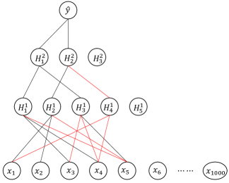
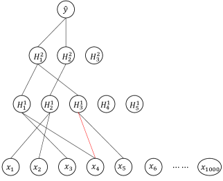
Figure 1: The left and right panels show the network structures selected for one dataset after the stages of training and retraining, respectively, where the black lines show the connections that are selected and exist in the true model, and the red lines show the connections that are selected but do not exist in the true model.

4.1.2 Nonlinear Regression

We generated 10 datasets from the following model:

$$y=\frac{5x_{2}}{1+x_{1}^{2}}+5\sin(x_{3}x_{4})+2x_{5}+0x_{6}+\cdots+0x_{2000}+\varepsilon,$$ (17)

where $\varepsilon\sim N(0,1)$ and is independent of $x_{i}$’s. We modeled the data by a 3-hidden layer neural network, which has 6, 4, and 3 hidden units on the first, second and third hidden layers, respectively. The tanh was used as the activation function. For each dataset, we ran SGD for 80,000 iterations to train the neural network with a learning rate of $\epsilon_{t}={0.005}$. The subsample size was set to 500. For the mixture Gaussian prior, we set $\sigma_{1,n}=0.01$, $\sigma_{0,n}=0.0001$, and $\lambda_{n}=0.00001$. The number of independent tries was set to $T=10$. After structure selection, the DNN was retrained using SGD for 40,000 iterations.

For comparison, the Spinn, dropout and DPF methods were also applied to this example with the same DNN structure and the same activation function. For Spinn, the regularization parameter for the weights in the first layer was tuned from the set $\{0.01,0.02,\dots,0.1\}$. For a fair comparison, it was also retrained for 40,000 iterations after structure selection as for the proposed method. For dropout, we set the dropout rate to be 0.2 for the first layer and 0.5 for the other layers. For DPF, we set the target pruning ratio to the ideal value 0.688%, which is the ratio of the number of connections related to true variables and the total number of connections, i.e. $(12053-1995\times 6)/12053$ with 12053 being the total number of connections including the biases. The results were summarized in Table 1.

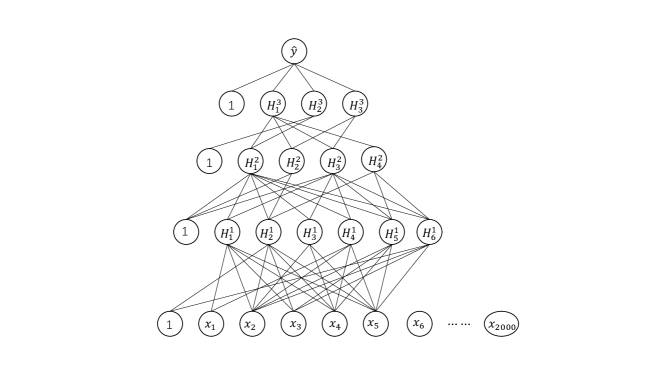
Figure 2: A network structure selected by the Bayesian evidence method for a simulated dataset from model (17), where the node ‘1’ denotes the bias term.

Table 1: Comparison of different methods for the simulated nonlinear regression example, where MSFE and MSPE were calculated by averaging over 10 datasets with the standard deviation given in the parentheses.

Activation	Method	$|\hat{S}|$	FSR	NSR	MSFE	MSPE
	BNN	5(0)	0	0	2.372(0.093)	2.439(0.132)
	Spinn	36.1(15.816)	0.861	0	3.090(0.194)	3.250(0.196)
Tanh	DPF	55.6(1.002)	0.910	0	2.934(0.132)	3.225(0.524)
	dropout	—	—	—	10.491(0.078)	13.565(0.214)
	BNN	5(0)	0	0	2.659(0.098)	2.778(0.111)
	Spinn	136.3(46.102)	0.963	0	3.858(0.243)	4.352(0.171)
ReLU	DPF	67.8(1.606)	0.934	0	5.893(0.619)	6.252(0.480)
	dropout	—	—	—	17.279(0.571)	18.630(0.559)

Table 1 indicates that the proposed BNN method significantly outperforms the Spinn and DPF methods in both prediction and variable selection. For this example, BNN can correctly identify the 5 true variables of the nonlinear regression (17), while Spinn and DPF identified too many false variables. Figure 2 shows the structure of a selected neural network by the BNN method. In terms of prediction, BNN, Spinn and DPF all significantly outperform the dropout method. In our experience, when irrelevant features are present in the data, learning a sparse DNN is always rewarded in prediction.

Figure 3 explores the relationship between Bayesian evidence and prediction accuracy. Since we set the number of tries $T=10$ for each of the 10 datasets, there are a total of 100 pairs of (Bayesian evidence, prediction error) shown in the plot. The plot shows a strong linear pattern that the prediction error of the sparse neural network decreases as Bayesian evidence increases. This justifies the rationale of Algorithm 1, where Bayesian evidence is employed for eliciting sparse neural network models learned by an optimization method in multiple runs with different initializations.

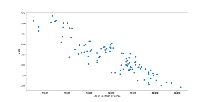
Figure 3: Scatter plot of MSPE versus the logarithm of Bayesian Evidence, for which the fitted OLS regression line is $y=-2.459\times 10^{-4}x-1.993$ with $R^{2}=0.8037$ and $p$-value = $2.2\times 10^{-16}$.

For this example, we have also compared different methods with the ReLU activation. The same network structure and the same hyperparameter setting were used as in the experiments with the tanh activation.The results are also summarized in Table 1, which indicate that the proposed BNN method still significantly outperforms the competing ones.

4.1.3 Nonlinear Classification

We generated 10 datasets from the following nonlinear system:

$$\begin{split}y=\begin{cases}\begin{array}[]{c}1\\ 0\end{array}&\begin{array}[]{c}e^{x_{1}}+x_{2}^{2}+5\sin(x_{3}x_{4})-3+0x_{5}+\cdots+0x_{1000}>0,\\ {\rm otherwise}.\end{array}\end{cases}\end{split}$$

Each dataset consisted of half of the observations with the response $y=1$. We modeled the data by a 3-hidden layer logistic regression neural network, which had 6,4,3 hidden units on the first, second and third hidden layers, respectively. The tanh was used as the activation function. The proposed method was compared with Spinn, dropout and DPF. For all the methods, the same hyperparameter values were used as in the nonlinear regression example of Section 4.1.2. The results are summarized in Table 2, which shows that the proposed method can identify the true variable for the nonlinear system and make more accurate prediction than Spinn, dropout and DPF. Compared to BNN and Spinn, DPF missed some true variables and produced a larger value of NSR.

Table 2: Comparison of different methods for the simulated classification example, where FA and PA were calculated by averaging over 10 datasets with the standard deviation given in the parentheses.

Method	$|\hat{S}|$	FSR	NSR	FA	PA
BNN	4(0)	0	0	0.8999(0.0023)	0.8958(0.0039)
Spinn	4.1(0.09)	0.024	0	0.8628(0.0009)	0.8606(0.0036)
DPF	61.9(0.81)	0.935	0.333	0.8920(0.0081)	0.8697(0.0010)
dropout	—	—	—	0.4898(0.0076)	0.4906(0.0071)

4.2 Residual Network Compression

This section assessed the performance of the proposed BNN method on network compression with CIFAR-10 (Krizhevsky et al., 2009) used as the illustrative dataset. The CIFAR-10 dataset is a benchmark dataset for computer vision, which consists of 10 classes, 50,000 training images, and 10,000 testing images. We modeled the data using both ResNet20 and ResNet32 (He et al., 2016) and then pruned them to different sparsity levels. We compared the proposed BNN method with DPF (Lin et al., 2020), dynamic sparse reparameterization (DSR) (Mostafa and Wang, 2019), sparse momentum (SM) (Dettmers and Zettlemoyer, 2019), and Variational Bayes(VB) (Blundell et al., 2015). All experiments were implemented using Pytorch (Paszke et al., 2017).

In all of our experiments, we followed the same training setup as used in Lin et al. (2020), i.e. the model was trained using SGD with momentum for 300 epochs, the data augmentation strategy (Zhong et al., 2017) was employed, the mini-batch size was set to 128, the momentum parameter was set to 0.9, and the initial learning rate was set to 0.1. We divided the learning rate by 10 at epoch 150 and 225. For the proposed method, we set the number of independent trials $T=10$, and used BIC to elicit sparse networks. In each trial, the mixture normal prior was imposed on the network weights after 150 epochs. After pruning, the model was retrained for one epoch for refining the nonzero weights. For the mixture normal prior, we set $\sigma_{1,n}^{2}=0.02$ and tried different values for $\sigma_{0,n}$ and $\lambda_{n}$ to achieve different sparsity levels. For ResNet-20, to achieve 10% target sparsity, we set $\sigma_{0,n}^{2}=4e-5$ and $\lambda_{n}=1e-6$; to achieve 20% target sparsity, we set $\sigma_{0,n}^{2}=6e-6$ and $\lambda_{n}=1e-7$. For ResNet-32, to achieve 5% target sparsity, we set $\sigma_{0,n}^{2}=6e-5$ and $\lambda_{n}=1e-7$; to achieve 10% target sparsity, we set $\sigma_{0,n}^{2}=2e-5$ and $\lambda_{n}=1e-5$.

Following the experimental setup in Lin et al. (2020), all experiments were run for 3 times and the averaged test accuracy and standard deviation were reported. For the VB method, we followed Blundell et al. (2015) to impose a mixture Gaussian prior (the same prior as used in our method) on the connection weights, and employed a diagonal multivariate Gaussian distribution to approximate the posterior. As in Blundell et al. (2015), we ordered the connection weights in the signal-to-noise ratio $\frac{|\mu|}{\sigma}$, and identified a sparse structure by removing the weights with a low signal-to-noise ratio. The results were summarized in Table 3, where the results of other baseline methods were taken from Lin et al. (2020). The comparison indicates that the proposed method is able to produce better prediction accuracy than the existing methods at about the same level of sparsity, and that the VB method is not very competitive in statistical inference although it is very attractive in computation. Note that the proposed method provides a one-shot pruning strategy. As discussed in Han et al. (2015b), it is expected that these results can be further improved with appropriately tuned hyperparameters and iterative pruning and retraining.

Table 3: Network compression for CIFAR-10 data, where the number in the parentheses denotes the standard deviation of the respective estimate.

	ResNet-20			ResNet-32
Method	Pruning Ratio	Test Accuracy		Pruning Ratio	Test Accuracy
BNN	19.673%(0.054%)	92.27(0.03)		9.531%(0.043%)	92.74(0.07)
SM	20%	91.54(0.16)		10%	91.54(0.18)
DSR	20%	91.78(0.28)		10%	91.41(0.23)
DPF	20%	92.17(0.21)		10%	92.42(0.18)
VB	20%	90.20(0.04)		10%	90.11(0.06)
BNN	9.546%(0.029%)	91.27(0.05)		4.783%(0.013%)	91.21(0.01)
SM	10%	89.76(0.40)		5%	88.68(0.22)
DSR	10%	87.88(0.04)		5%	84.12(0.32)
DPF	10%	90.88(0.07)		5%	90.94(0.35)
VB	10%	89.33(0.16)		5%	88.14(0.04)

The CIFAR-10 has been used as a benchmark example in many DNN compression experiments. Other than the competing methods considered above, the targeted dropout method (Gomez et al., 2019) reported a Resnet32 model with 47K parameters (90% sparsity) and the prediction accuracy 91.48%. The Bayesian compression method with a group normal-Jeffreys prior (BC-GNJ) (Louizos et al., 2017) reported a VGG16 model, a very deep convolutional neural network model proposed by Simonyan and Zisserman (2014), with 9.2M parameters (93.3% sparsity) and the prediction accuracy 91.4%. A comparison with our results reported in Table 3 indicates again the superiority of the proposed BNN method.

Finally, we note that the proposed BNN method belongs to the class of pruning methods and it provides an effective way for learning sparse DNNs. Contemporary experience shows that directly training a sparse or small dense network from the start typically converges slower than training with a pruning method, see e.g. Frankle and Carbin (2018)Ye et al. (2020). This issue can be illustrated using a network compression example. Three experiments were conducted for a ResNe20 (with 10% sparsity level) on the CIFAR 10 dataset: (a) sparse BNN, i.e., running the proposed BNN method with randomly initialized weights; (b) starting with sparse network, i.e., training the sparse network learned by the proposed BNN method but with the weights randomly reinitialized; and (c) starting with small dense network, i.e., training a network whose number of parameters in each layer is about the same as that of the sparse network in experiment (b) and whose weights are randomly initialized. The experiment (a) consisted of 400 epochs, where the last 100 epochs were used for refining the nonzero-weights of the sparse network obtained at epoch 300 via connection sparsification. Both the experiments (b) and (c) consisted of 300 epochs. In each of the experiments, the learning rate was set in the standard scheme (Lin et al., 2020), i.e., started with 0.1 and then decreased by a factor of 10 at epochs 150 and 225, respectively. For random initialization, we used the default method in PyTorch (He et al., 2015). For example, for a 2-D convolutional layer with $n_{in}$ input feature map channels, $n_{out}$ output feature map channels, and a convolutional kernel of size $w\times h$, the weights and bias of the layer were initialized by independent draws from the uniform distribution $Unif(-\frac{1}{\sqrt{n_{in}\times w\times h}},\frac{1}{\sqrt{n_{in}\times w\times h}})$.

Figure 4 shows the training and testing paths obtained in the three experiments. It indicates that the sparse neural network learned by the proposed method significantly outperforms the other two networks trained with randomly initialized weights. This result is consistent with the finding of Frankle and Carbin (2018) that the architectures uncovered by pruning are harder to train from the start and they often reach lower accuracy than the original neural networks.

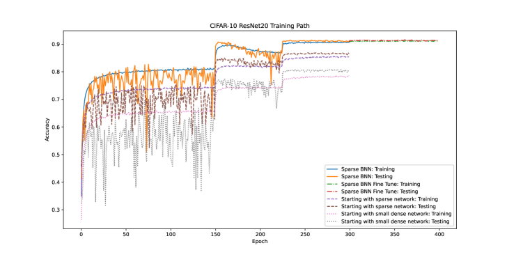
Figure 4: Training and testing paths of a ResNet20 model (with 10% sparsity level) on the CIFAR-10 dataset: “Sparse BNN: Training” is the path for fitting the full neural network in experiment (a) (for epochs 1-300); “Sparse BNN Fine Tune: Training” is the path for refining the nonzero-weights of the sparse network obtained in experiment (a) via connection sparsification (for epochs 301-400); “Starting with sparse network: Training” is the path for fitting a sparse neural network in experiment (b); and “Starting with small dense network: Training” is the path for fitting a small dense neural network in experiment (c). The curves for testing can be interpreted similarly.

Regarding this experiment, we have further two remarks. First, the nonzero weights refining step in Algorithm 1 can consist of a few epochs only. This step is mainly designed for a theoretical purpose, ensuring the followed evidence evaluation to be done on a local mode of the posterior. In terms of sparse neural network learning, the mixture Gaussian prior plays a key role in sparsifying the neural network, while the nonzero weights refining step is not essential. As illustrated by Figure 4, this step did not significantly improve the training and testing errors of the sparse neural network. Second, as mentioned previously, the proposed BNN method falls into the class of pruning methods suggested by Frankle and Carbin (2018) for learning sparse DNNs. Compared to the existing pruning methods, the proposed method is more theoretically sound, which ensures the resulting sparse network to possess nice theoretical properties such as posterior consistency, variable selection consistency and asymptotically optimal generalization bounds.

5 Discussion

This paper provides a complete treatment for sparse DNNs in both theory and computation. The proposed method works like a frequentist method, but is justified under the Bayesian framework. With the proposed method, a sparse neural network with at most $O(n/\log(n))$ connections could be learned via sparsifying an over-parameterized one. Such a sparse neural network has nice theoretical properties, such as posterior consistency, variable selection consistency, and asymptotically optimal generalization bound.

In computation, we proposed to use Bayesian evidence or BIC for eliciting sparse DNN models learned by an optimization method in multiple runs with different initializations. Since conventional optimization methods such as SGD and Adam (Kingma and Ba, 2014) can be used to train the DNNs, the proposed method is computationally more efficient than the standard Bayesian method. Our numerical results show that the proposed method can perform very well in large-scale network compression and high-dimensional nonlinear variable selection. The networks learned by the proposed method tend to predict better than the existing methods.

Regarding the number of runs of the optimization method, i.e., the value of $T$, in Algorithm 1, we would note again that Algorithm 1 is not very sensitive to it. For example, for the nonlinear regression example, Algorithm 1 correctly identified the true variables in each of the 10 runs. For the CIFAR-10 example with ResNet20 and 10% target sparsity level, Algorithm 1 achieved the test accuracies in 10 runs: $91.09\%,91.16\%,91.17\%,91.18\%,91.18\%,91.24\%$, $91.24\%,91.24\%,91.27\%,91.31\%$ (in ascending order), where the worst one is still better than those achieved by the baseline methods.

In this work, we choose the two-mixture Gaussian prior for the weights and biases of the DNN, mainly for the sake of computational convenience. Other choices, such as two-mixture Laplace prior (Ročková, 2018), which will lead to the same posterior contraction with an appropriate choice for the prior hyperparameters. To be more specific, Theorem S1 (in the supplementary material) establishes sufficient conditions that guarantee the posterior consistency, and any prior distribution satisfying the sufficient conditions can yield consistent posterior inferences for the DNN.

Beyond the absolutely continuous prior, the hierarchical prior used in Liang et al. (2018) and Polson and Ročková (2018) can be adopted for DNNs. To be more precise, one can assume that

$$\boldsymbol{\beta}_{\boldsymbol{\gamma}}\mid\boldsymbol{\gamma}\sim N(0,\sigma_{1,n}^{2}\boldsymbol{I}_{\left|\boldsymbol{\gamma}\right|\times\left|\boldsymbol{\gamma}\right|}),\quad{\boldsymbol{\beta}}_{{\boldsymbol{\gamma}}^{c}}=0;$$ (18)

$$\pi(\boldsymbol{\gamma})\propto\lambda_{n}^{\left|\boldsymbol{\gamma}\right|}\left(1-\lambda_{n}\right)^{K_{n}-\left|\boldsymbol{\gamma}\right|}\boldsymbol{1}\left\{1\leq\left|\boldsymbol{\gamma}\right|\leq\bar{r}_{n},\boldsymbol{\gamma}\in\mathcal{G}\right\},$$ (19)

where ${\boldsymbol{\beta}}_{{\boldsymbol{\gamma}}^{c}}$ is the complement of ${\boldsymbol{\beta}}_{{\boldsymbol{\gamma}}}$, $\left|\boldsymbol{\gamma}\right|$ is the number of nonzero elements of $\boldsymbol{\gamma}$, $\boldsymbol{I}_{\left|\boldsymbol{\gamma}\right|\times\left|\boldsymbol{\gamma}\right|}$ is a $\left|\boldsymbol{\gamma}\right|\times\left|\boldsymbol{\gamma}\right|$ identity matrix, $\bar{r}_{n}$ is the maximally allowed size of candidate networks, $\mathcal{G}$ is the set of valid DNNs, and the hyperparameter $\lambda_{n}$, as in (4), can be read as an approximate prior probability for each connection or bias to be included in the DNN. Under this prior, the product of the weight or bias and its indicator follows a discrete spike-and-slab prior distribution, i.e.

$${{\boldsymbol{w}}}_{ij}^{h}{\boldsymbol{\gamma}}_{ij}^{\boldsymbol{w}^{h}}|{\boldsymbol{\gamma}}_{ij}^{\boldsymbol{w}^{h}}\sim{\boldsymbol{\gamma}}_{ij}^{\boldsymbol{w}^{h}}N(0,\sigma_{1,n}^{2})+(1-{\boldsymbol{\gamma}}_{ij}^{\boldsymbol{w}^{h}})\delta_{0},\ \ {{\boldsymbol{b}}}_{k}^{h}{\boldsymbol{\gamma}}_{k}^{\boldsymbol{b}^{h}}|{\boldsymbol{\gamma}}_{k}^{\boldsymbol{b}^{h}}\sim{\boldsymbol{\gamma}}_{k}^{\boldsymbol{b}^{h}}N(0,\sigma_{1,n}^{2})+(1-{\boldsymbol{\gamma}}_{k}^{\boldsymbol{b}^{h}})\delta_{0},$$

where $\delta_{0}$ denotes the Dirac delta function. Under this hierarchical prior, it is not difficult to show that the posterior consistency and structure selection consistency theory developed in this paper still hold. However, from the computational perspective, the hierarchical prior might be inferior to the mixture Gaussian prior adopted in the paper, as the posterior $\pi({\boldsymbol{\beta}}_{{\boldsymbol{\gamma}}},{\boldsymbol{\gamma}}|D_{n})$ is hard to be optimized or simulated from. It is known that directly simulating from $\pi({\boldsymbol{\beta}}_{{\boldsymbol{\gamma}}},{\boldsymbol{\gamma}}|D_{n})$ using an acceptance-rejection based MCMC algorithm can be time consuming. A feasible way is to formulate the prior of ${\boldsymbol{\beta}}_{{\boldsymbol{\gamma}}}$ as ${\boldsymbol{\beta}}_{{\boldsymbol{\gamma}}}={\boldsymbol{\theta}}\otimes{\boldsymbol{\gamma}}$, where ${\boldsymbol{\theta}}\sim N(0,\sigma^{2}_{1,n}I_{H_{n}\times H_{n}})$ can be viewed as a latent variable and $\otimes$ denotes entry-wise product. Then one can first simulate from the marginal posterior $\pi({\boldsymbol{\theta}}|D_{n})$ using a stochastic gradient MCMC algorithm and then make inference of the network structure based on the conditional posterior $\pi({\boldsymbol{\gamma}}|{\boldsymbol{\theta}},D_{n})$. We note that the gradient $\nabla_{{\boldsymbol{\theta}}}\log\pi({\boldsymbol{\theta}}|D^{n})$ can be approximated based on the following identity developed in Song et al. (2020),

$$\nabla_{{\boldsymbol{\theta}}}\log\pi({\boldsymbol{\theta}}|D^{n})=\sum_{{\boldsymbol{\gamma}}}\pi({\boldsymbol{\gamma}}|{\boldsymbol{\theta}},D^{n})\nabla_{{\boldsymbol{\theta}}}\log\pi({\boldsymbol{\theta}}|{\boldsymbol{\gamma}},D^{n}),$$

where $D_{n}$ can be replaced by a dataset duplicated with mini-batch samples if the subsampling strategy is used to accelerate the simulation. This identity greatly facilitates the simulations for the dimension jumping problems, which requires only some samples to be drawn from the conditional posterior $\pi({\boldsymbol{\gamma}}|{\boldsymbol{\theta}},D^{n})$ for approximating the gradient $\nabla_{{\boldsymbol{\theta}}}\log\pi({\boldsymbol{\theta}}|D^{n})$ at each iteration. A further exploration of this discrete prior for its use in deep learning is of great interest, although there are some difficulties needing to be addressed in computation.

Supplementary Material

This material is organized as follows. Section S1 gives the proofs on posterior consistency, Section S2 gives the proofs on structure selection consistency, Section S3 gives the proofs on generalization bounds, and Section S4 gives some mathematical facts of the sparse DNN.

S1 Proofs on Posterior Consistency

S1.1 Basic Formulas of Bayesian Neural Networks

Normal Regression.

Let $p_{\mu}$ denote the density of $N(\mu,\sigma^{2})$ where $\sigma^{2}$ is a known constant, and let $p_{{\boldsymbol{\beta}}}$ denote the density of $N(\mu({\boldsymbol{\beta}},{\boldsymbol{x}}),\sigma^{2})$. Extension to the case $\sigma^{2}$ is unknown is simple by following the arguments given in Jiang (2007). In this case, an inverse gamma prior can be assumed for $\sigma^{2}$ as suggested by Jiang (2007). Define the Kullback-Leibler divergence as $d_{0}(p,p^{*})=\int p^{*}\log(p^{*}/p)$ for two densities $p$ and $p^{*}$. Define a distance $d_{t}(p,p^{*})=t^{-1}(\int p^{*}(p^{*}/p)^{t}-1)$ for any $t>0$, which decreases to $d_{0}$ as $t$ decreases toward 0. A straightforward calculation shows

$$d_{1}(p_{\mu_{1}},p_{\mu_{2}})=\int p_{\mu_{1}}(p_{\mu_{1}}/p_{\mu_{1}})-1=\exp\left(\frac{1}{\sigma^{2}}(\mu_{2}-\mu_{1})^{2}\right)-1=\frac{1}{\sigma^{2}}(\mu_{2}-\mu_{1})^{2}+o((\mu_{2}-\mu_{1})^{3}),$$ (S1)

$$d_{0}(p_{1},p_{2})=\frac{1}{2\sigma^{2}}(\mu_{1}-\mu_{2})^{2}.$$ (S2)

Logistic Regression.

Let $p_{\mu}$ denote the probability mass function with the success probability given by $1/(1+e^{-\mu})$. Similarly, we define $p_{{\boldsymbol{\beta}}}$ as the logistic regression density for a binary classification DNN with parameter ${\boldsymbol{\beta}}$. For logistic regression, we have

$$d_{1}(p_{\mu_{1}},p_{\mu_{2}})=\int p_{\mu_{2}}(p_{\mu_{2}}/p_{\mu_{1}})-1=\frac{e^{2\mu_{2}-\mu_{1}}+e^{\mu_{1}}-2e^{\mu_{2}}}{(1+e^{\mu_{2}})^{2}},$$

which, by the mean value theorem, can be written as

$$d_{1}(p_{\mu_{1}},p_{\mu_{2}})=\frac{e^{\mu^{\prime}}-e^{2\mu_{2}-\mu^{\prime}}}{(1+e^{\mu_{2}})^{2}}(\mu_{\mu_{1}}-\mu_{2})=\frac{e^{\mu^{\prime}}(1-e^{2\mu_{2}-2\mu^{\prime}})}{(1+e^{\mu_{2}})^{2}}(\mu_{1}-\mu_{2}),$$

where $\mu^{\prime}$ denotes an intermediate point between $\mu_{1}$ and $\mu_{2}$, and thus $|\mu^{\prime}-\mu_{2}|\leq|\mu_{1}-\mu_{2}|$. Further, by Taylor expansion, we have

$$e^{\mu^{\prime}}=e^{\mu_{2}}[1+(\mu^{\prime}-\mu_{2})+O((\mu^{\prime}-\mu_{2})^{2})],\quad e^{2\mu_{2}-2\mu^{\prime}}=1+2(\mu_{2}-\mu^{\prime})+O((\mu_{2}-\mu^{\prime})^{2}).$$

Therefore,

$$d_{1}(p_{\mu_{1}},p_{\mu_{2}})\leq\frac{e^{\mu_{2}}}{(1+e^{\mu_{2}})^{2}}\left[2|\mu_{2}-\mu^{\prime}|+O((\mu_{2}-\mu^{\prime})^{2})\right]|\mu_{1}-\mu_{2}|\leq\frac{1}{2}(\mu_{1}-\mu_{2})^{2}+O((\mu_{1}-\mu_{2})^{3}),$$ (S3)

and

$$d_{0}(p_{u},p_{v})=\int p_{v}(\log p_{v}-\log p_{u})v_{y}(dy)=\log(1+e^{\mu_{u}})-\log(1+e^{\mu_{v}})+\frac{e^{\mu_{v}}}{1+e^{\mu_{v}}}(\mu_{v}-\mu_{u}).$$

By the mean value theorem, we have

$$d_{0}(p_{u},p_{v})=\frac{e^{\mu^{\prime}}}{1+e^{\mu^{\prime}}}(\mu_{u}-\mu_{v})+\frac{e^{\mu_{v}}}{1+e^{\mu_{v}}}(\mu_{v}-\mu_{u})=[\frac{e^{\mu_{v}}}{1+e^{\mu_{v}}}-\frac{e^{\mu^{\prime}}}{1+e^{\mu^{\prime}}}](\mu_{v}-\mu_{u}),$$ (S4)

where $\mu^{\prime}$ denotes an intermediate point between $\mu_{u}$ and $\mu_{v}$.

S1.2 Posterior Consistency of General Statistical Models

We first introduce a lemma concerning posterior consistency of general statistical models. This lemma has been proved in Jiang (2007). Let $\mathbb{P}_{n}$ denote a sequence of sets of probability densities, let $\mathbb{P}_{n}^{c}$ denote the complement of $\mathbb{P}_{n}$, and let $\epsilon_{n}$ denote a sequence of positive numbers. Let $N(\epsilon_{n},\mathbb{P}_{n})$ be the minimum number of Hellinger balls of radius $\epsilon_{n}$ that are needed to cover $\mathbb{P}_{n}$, i.e., $N(\epsilon_{n},\mathbb{P}_{n})$ is the minimum of all $k$’s such that there exist sets $S_{j}=\{p:d(p,p_{j})\leq\epsilon_{n}\}$, $j=1,\ldots,k$, with $\mathbb{P}_{n}\subset\cup_{j=1}^{k}S_{j}$ holding, where $d(p,q)=\sqrt{\int(\sqrt{p}-\sqrt{q})^{2}}$ denotes the Hellinger distance between the two densities $p$ and $q$.

Let $D_{n}=(z^{(1)},\ldots,z^{(n)})$ denote the dataset, where the observations $z^{(1)},\ldots,z^{(n)}$ are iid with the true density $p^{*}$. The dimension of $z^{(1)}$ and $p^{*}$ can depend on $n$. Define $\pi(\cdot)$ as the prior density, and $\pi(\cdot|D_{n})$ as the posterior. Define $\hat{\pi}(\epsilon)=\pi[d(p,p^{*})>\epsilon|D_{n}]$ for each $\epsilon>0$. Define the KL divergence as $d_{0}(p,p^{*})=\int p^{*}\log(p^{*}/p)$. Define $d_{t}(p,p^{*})=t^{-1}(\int p^{*}(p^{*}/p)^{t}-1)$ for any $t>0$, which decreases to $d_{0}$ as $t$ decreases toward 0. Let $P^{*}$ and $E^{*}$ denote the probability measure and expectation for the data $D_{n}$, respectively. Define the conditions:

• $\log N(\epsilon_{n},\mathbb{P}_{n})\leq n\epsilon_{n}^{2}$ for all sufficiently large $n$;

• $\pi(\mathbb{P}_{n}^{c})\leq e^{-bn\epsilon_{n}^{2}}$ for all sufficiently large $n$;

• $\pi[p:d_{t}(p,p^{*})\leq b^{\prime}\epsilon_{n}^{2}]\geq e^{-b^{\prime}n\epsilon_{n}^{2}}$ for all sufficiently large $n$ and some $t>0$,

where $2>b>2b^{\prime}>0$ are positive constants. The following lemma is due to the same argument of Jiang (2007, Proposition 1).

Lemma S1.

Under the conditions (a), (b) and (c) (for some $t>0$), given sufficiently large $n$, we have

• $P^{*}\left[\hat{\pi}(4\epsilon_{n})\geq 2e^{-0.5n\epsilon_{n}^{2}\min\{1,2-x,b-x,t(x-2b^{\prime})\}}\right]\leq 2e^{-0.5n\epsilon_{n}^{2}\min\{1,2-x,b-x,t(x-2b^{\prime})\}}$,

• $E^{*}\hat{\pi}(4\epsilon_{n})\leq 4e^{-n\epsilon_{n}^{2}\min\{1,2-x,b-x,t(x-2b^{\prime})\}}$.

for any $2b^{\prime}<x<b$.

S1.3 General Shrinkage Prior Settings for Deep Neural Networks

Let ${\boldsymbol{\beta}}$ denote the vector of parameters, including the weights of connections and the biases of the hidden and output units, of a deep neural network. Consider a general prior setting that all entries of ${\boldsymbol{\beta}}$ are subject to independent continuous prior $\pi_{b}$, i.e., $\pi({\boldsymbol{\beta}})=\prod_{j=1}^{K_{n}}\pi_{b}(\beta_{j})$. Theorem S1 provides a sufficient condition for posterior consistency.

Theorem S1 (Posterior consistency).

Assume the conditions A.1, A.2 and A.3 hold, if the prior $\pi({\boldsymbol{\beta}})$ satisfies that

$$\log(1/\underline{\pi}_{b})=O(H_{n}\log n+\log\overline{L}),$$ (S5)

$$\pi_{b}\{[-\eta_{n},\eta_{n}]\}\geq 1-\frac{1}{K_{n}}\exp\{-\tau[H_{n}\log n+\log\overline{L}+\log p_{n}]\}\mbox{ and }\pi_{b}\{[-\eta_{n}^{\prime},\eta_{n}^{\prime}]\}\geq 1-\frac{1}{K_{n}},$$ (S6)

$$-\log[K_{n}\pi_{b}(|\beta_{j}|>M_{n})]\succ n\epsilon_{n}^{2},$$ (S7)

for some $\tau>0$, where $\eta_{n}<1/\{\sqrt{n}K_{n}(n/H_{n})^{H_{n}}(c_{0}M_{n})^{H_{n}}\}$, $\eta_{n}^{\prime}<1/\{\sqrt{n}K_{n}(r_{n}/H_{n})^{H_{n}}(c_{0}E_{n})^{H_{n}}\}$ with some $c_{0}>1$, $\underline{\pi}_{b}$ is the minimal density value of $\pi_{b}$ within interval $[-E_{n}-1,E_{n}+1]$, and $M_{n}$ is some sequence satisfying $\log(M_{n})=O(\log(n))$. Then, there exists a sequence $\epsilon_{n}$, satisfying $n\epsilon_{n}^{2}\asymp r_{n}H_{n}\log n+r_{n}\log\overline{L}+s_{n}\log p_{n}+n\varpi_{n}^{2}$ and $\epsilon_{n}\prec 1$, such that

$$\begin{split}&P^{*}\left\{\pi[d(p_{{\boldsymbol{\beta}}},p_{\mu^{*}})>4\epsilon_{n}|D_{n}]\geq 2e^{-nc\epsilon_{n}^{2}}\right\}\leq 2e^{-cn\epsilon_{n}^{2}},\\ &E_{D_{n}}^{*}\pi[d(p_{{\boldsymbol{\beta}}},p_{\mu^{*}})>4\epsilon_{n}|D_{n}]\leq 4e^{-2cn\epsilon_{n}^{2}}.\end{split}$$ (S8)

for some $c>0$.

To prove Theorem S1, we first introduce a useful Lemma:

Lemma S2 (Theorem 1 of Zubkov and Serov (2013)).

Let $X\sim\mbox{B}(n,v)$ be a Binomial random variable. For any $1<k<n-1$,

$$Pr(X\geq k+1)\leq 1-\Phi(\mbox{sign}(k-nv)\{2nH(v,k/n)\}^{1/2}),$$

where $\Phi$ is the cumulative distribution function (CDF) of the standard Gaussian distribution and $H(v,k/n)=(k/n)\log(k/nv)+(1-k/n)\log[(1-k/n)/(1-v)]$.

Proof of Theorem S1

Theorem S1 can be proved using Lemma S1, so it suffices to verify conditions (a)-(c) given in Section S1.2.

Checking condition (c) for $t=1$:

Consider the set $A=\{{\boldsymbol{\beta}}:\max_{j\in{\boldsymbol{\gamma}}^{*}}\|\beta_{j}-\beta_{j}^{*}\|_{\infty}\leq\omega_{n},\max_{j\notin{\boldsymbol{\gamma}}^{*}}\|\beta_{j}-\beta_{j}^{*}\|_{\infty}\leq\omega_{n}^{\prime}\}$, where $\omega_{n}={c_{1}\epsilon_{n}}/[H_{n}(r_{n}/H_{n})^{H_{n}}(c_{0}E_{n})^{H_{n}}]$ and $\omega_{n}^{\prime}={c_{1}\epsilon_{n}}/[K_{n}(r_{n}/H_{n})^{H_{n}}(c_{0}E_{n})^{H_{n}}]$ for some constant $c_{1}>0$ and $c_{0}>1$. If ${\boldsymbol{\beta}}\in A$, then by Lemma S2, we have $|\mu({\boldsymbol{\beta}},{\boldsymbol{x}})-\mu({\boldsymbol{\beta}}^{*},{\boldsymbol{x}})|\leq 3{c_{1}\epsilon_{n}}$. By condition A.2.1, $|\mu({\boldsymbol{\beta}},{\boldsymbol{x}})-\mu^{*}({\boldsymbol{x}})|\leq 3{c_{1}\epsilon_{n}}+\varpi_{n}$. Combining it with (S1)–(S4), for both normal and logistic models, we have

$$d_{1}(p_{{\boldsymbol{\beta}}},p_{\mu^{*}})\leq C(1+o(1))E_{x}(\mu({\boldsymbol{\beta}},{\boldsymbol{x}})-\mu^{*}({\boldsymbol{x}}))^{2}\leq C(1+o(1))(3{c_{1}\epsilon_{n}}+\varpi_{n})^{2},\quad\mbox{ if }{\boldsymbol{\beta}}\in A,$$

for some constant $C$. Thus for any small $b^{\prime}>0$, condition (c) holds as long as that $c_{1}$ is sufficiently small, $n\epsilon_{n}^{2}\geq M_{0}n\varpi_{n}^{2}$ for large $M_{0}$, and the prior satisfies $-\log\pi(A)\leq b^{\prime}{n\epsilon_{n}^{2}}$.

Since $\pi(A)\geq(2\underline{\pi}_{b}\omega_{n})^{r_{n}}\times\pi(\{\max_{j\notin{\boldsymbol{\gamma}}^{*}}\|\beta_{j}\|\leq\omega_{n}^{\prime}\})$, $\pi_{b}([-\omega_{n}^{\prime},\omega_{n}^{\prime}])\geq 1-1/K_{n}$ (due to the fact $\omega_{n}^{\prime}\gg\eta_{n}^{\prime}$), and $\log(1/\omega_{n})\asymp\log(1/\epsilon_{n})+H_{n}\log E_{n}+H_{n}\log(r_{n}/H_{n})+\mbox{constant}=O(H_{n}\log n)$ (note that $\log(1/\epsilon_{n})=O(\log n)$), the above requirement holds when $n\epsilon_{n}^{2}\geq M_{0}r_{n}H_{n}\log n$ for some sufficiently large constant $M_{0}$.

Checking condition (a):

Let $\mathbb{P}_{n}$ denote the set of all DNN models whose weight parameter ${\boldsymbol{\beta}}$ satisfies that

$${\boldsymbol{\beta}}\in B_{n}=\{|\beta_{j}|\leq M_{n},{\boldsymbol{\gamma}}_{\boldsymbol{\beta}}=\{i:|\beta_{i}|\geq\delta_{n}^{\prime}\}\mbox{ satisfies }|{\boldsymbol{\gamma}}_{\boldsymbol{\beta}}|\leq k_{n}r_{n}\mbox{ and }|{\boldsymbol{\gamma}}_{\boldsymbol{\beta}}|_{in}\leq k_{n}^{\prime}s_{n}\},$$ (S9)

where $|{\boldsymbol{\gamma}}|_{in}$ denotes the input dimension of sparse network ${\boldsymbol{\gamma}}$, $k_{n}(\leq n/r_{n})$ and $k_{n}^{\prime}(\leq n/s_{n})$ will be specified later, and $\delta_{n}=c_{1}\epsilon_{n}/[H_{n}(k_{n}r_{n}/H_{n})^{H_{n}}(c_{0}M_{n})^{H_{n}}]$ and $\delta_{n}^{\prime}=c_{1}\epsilon_{n}/[K_{n}(k_{n}r_{n}/H_{n})^{H_{n}}(c_{0}M_{n})^{H_{n}}]$ for some constant $c_{1}>0$ and $c_{0}>1$. Consider two parameter vectors ${\boldsymbol{\beta}}^{u}$ and ${\boldsymbol{\beta}}^{v}$ in set $B_{n}$, such that there exists a model ${\boldsymbol{\gamma}}$ with $|{\boldsymbol{\gamma}}|\leq k_{n}r_{n}$ and $|{\boldsymbol{\gamma}}|_{in}\leq k_{n}^{\prime}s_{n}$, and $|\beta^{u}_{j}-\beta^{v}_{j}|\leq\delta_{n}$ for all $j\in{\boldsymbol{\gamma}}$, $\max(|\beta_{j}^{u}|,|\beta_{j}^{v}|)\leq\delta_{n}^{\prime}$ for all $j\notin{\boldsymbol{\gamma}}$. Hence, by Lemma S2, we have that $|\mu({\boldsymbol{\beta}}^{u},{\boldsymbol{x}})-\mu({\boldsymbol{\beta}}^{v},{\boldsymbol{x}})|^{2}\leq 9c_{1}^{2}\epsilon_{n}^{2}$, and furthermore, due to (S1)-(S4), we can easily derive that

$$d(p_{{\boldsymbol{\beta}}^{u}},p_{{\boldsymbol{\beta}}^{v}})\leq\sqrt{d_{0}(p_{{\boldsymbol{\beta}}^{u}},p_{{\boldsymbol{\beta}}^{v}})}\leq\sqrt{(9+o(1))c_{1}^{2}C\epsilon_{n}^{2}}\leq\epsilon_{n},$$

for some $C$, given a sufficiently small $c_{1}$. On the other hand, if some ${\boldsymbol{\beta}}^{u}\in B_{n}$ and its connections whose magnitudes are larger than $\delta_{n}^{\prime}$ don’t form a valid network, then by Lemma S2 and (S1)-(S4), we also have that $d(p_{{\boldsymbol{\beta}}^{u}},p_{{\boldsymbol{\beta}}^{o}})\leq\epsilon_{n}$, where ${\boldsymbol{\beta}}^{o}=0$ denotes a empty output network.

Given the above results, one can bound the packing number $N(\mathbb{P}_{n},\epsilon_{n})$ by $\sum_{j=1}^{k_{n}r_{n}}{\cal X}^{j}_{H_{n}}\left(\frac{2M_{n}}{\delta_{n}}\right)^{j}$, where ${\cal X}^{j}_{H_{n}}$ denotes the number of all valid networks who has exact $j$ connection and has no more than $k_{n}^{\prime}s_{n}$ inputs. Since $\log{\cal X}^{j}_{H_{n}}\leq k_{n}^{\prime}s_{n}\log p_{n}+j\log(k_{n}^{\prime}s_{n}L_{1}+H_{n}\overline{L}^{2})$,

$$\begin{split}\log N(\mathbb{P}_{n},\epsilon_{n})&\leq\log k_{n}r_{n}+k_{n}r_{n}\log H_{n}+2k_{n}r_{n}\log(\overline{L}+k_{n}^{\prime}s_{n})+k_{n}^{\prime}s_{n}\log p_{n}\\ &+k_{n}r_{n}\log\frac{2M_{n}H_{n}(k_{n}r_{n}/H_{n})^{H_{n}}M_{n}^{H_{n}}}{c_{1}\epsilon_{n}}\\ &=k_{n}r_{n}*O\{H_{n}\log n+\log\overline{L}+\mbox{constant}\}+k_{n}^{\prime}s_{n}\log p_{n}\end{split}$$

where the second inequality is due to $\log M_{n}=O(\log n)$, $k_{n}r_{n}\leq n$ and $k_{n}^{\prime}s_{n}\leq n$. We can choose $k_{n}$ and $k_{n}^{\prime}$ such that $k_{n}r_{n}\{H_{n}\log n+\log\overline{L}\}\asymp k_{n}^{\prime}s_{n}\asymp n\epsilon_{n}^{2}$ and $\log N(\mathbb{P}_{n},\epsilon_{n})\leq n\epsilon_{n}^{2}$.

Checking condition (b):

$\pi(\mathbb{P}_{n}^{c})\leq Pr(\mbox{Binomial}(K_{n},v_{n})>k_{n}r_{n})+K_{n}\pi_{b}(|\beta_{j}|>M_{n})+Pr(|{\boldsymbol{\gamma}}_{\boldsymbol{\beta}}|_{in}\geq k_{n}^{\prime}s_{n})$, where $v_{n}=1-\pi_{b}([-\delta_{n}^{\prime},\delta_{n}^{\prime}])$. By the condition of $\pi_{b}$ and the fact that $\delta_{n}^{\prime}\gg\eta_{n}$, $v_{n}\leq\exp\{-\tau[H_{n}\log n+\log\overline{L}+\log p_{n})]-\log K_{n}\}$ for some positive constant $\tau$. Hence, by Lemma S2, $-\log Pr(\mbox{Binomial}(K_{n},v_{n})>k_{n}r_{n})\approx\tau k_{n}r_{n}[H_{n}\log n+\log\overline{L}+\log p_{n}]\gtrsim n\epsilon_{n}^{2}$ due to the choice of $k_{n}$, and $-\log Pr(|{\boldsymbol{\gamma}}_{\boldsymbol{\beta}}|_{in}\geq k_{n}^{\prime}s_{n})\approx k_{n}^{\prime}s_{n}[\tau(H_{n}\log n+\log\overline{L}+\log p_{n})+\log(K_{n}/L_{1}p_{n})]\gtrsim n\epsilon_{n}^{2}$ due to the choice of $k_{n}^{\prime}$. Thus, condition (b) holds as well.

S1.4 Proof of Theorem 2.1

Proof.

It suffices to verify the conditions listed in Theorem S1. Let $M_{n}=\max(\sqrt{2n}\sigma_{1,n},E_{n})$. Condition (S5) is due to $E_{n}^{2}/2\sigma_{1,n}^{2}+\log\sigma_{1,n}^{2}=O[H_{n}\log n+\log\overline{L}]$; Condition (S6) can be verified by $\lambda_{n}=1/\{K_{n}[n^{H_{n}}(\overline{L}p_{n})]^{\tau^{\prime}}\}$ and $\sigma_{0,n}\prec 1/\{\sqrt{n}K_{n}(n/H_{n})^{H_{n}}(c_{0}M_{n})^{H_{n}}\}$; Condition (S7) can be verified by $M_{n}\geq 2n\sigma_{0,n}^{2}$ and $\tau[H_{n}\log n+\log\overline{L}+\log p_{n}]+M_{n}^{2}/2\sigma_{1,n}^{2}\geq n$.

∎

S2 Proofs on Structure Selection Consistency

S2.1 Proof of Theorem 2.2

Proof.

$$\begin{split}&\max|q_{i}-e_{i|\nu({\boldsymbol{\gamma}}^{*},{\boldsymbol{\beta}}^{*})}|\leq\max\int\sum_{{\boldsymbol{\gamma}}}|e_{i|\nu({\boldsymbol{\gamma}},{\boldsymbol{\beta}})}-e_{i|\nu({\boldsymbol{\gamma}}^{*},{\boldsymbol{\beta}}^{*})}|\pi({\boldsymbol{\gamma}}|{\boldsymbol{\beta}},D_{n})\pi({\boldsymbol{\beta}}|D_{n})d{\boldsymbol{\beta}}\\ =&\max\int_{A(4\epsilon_{n})}\sum_{{\boldsymbol{\gamma}}}|e_{i|\nu({\boldsymbol{\gamma}},{\boldsymbol{\beta}})}-e_{i|\nu({\boldsymbol{\gamma}}^{*},{\boldsymbol{\beta}}^{*})}|\pi({\boldsymbol{\gamma}}|{\boldsymbol{\beta}},D_{n})\pi({\boldsymbol{\beta}}|D_{n})d{\boldsymbol{\beta}}+\rho(4\epsilon_{n})\\ \leq&\hat{\pi}(4\epsilon_{n})+\rho(4\epsilon_{n})\stackrel{{\scriptstyle p}}{{\rightarrow}}0,\end{split}$$ (S10)

where $\stackrel{{\scriptstyle p}}{{\to}}$ denotes convergence in probability, and $\hat{\pi}(c)$ denotes the posterior probability of the set $A(c)=\{{\boldsymbol{\beta}}:d(p_{\boldsymbol{\beta}},p_{\mu^{*}})\geq c\}$. The last convergence is due to the identifiability condition B.1 and the posterior consistency result. This completes the proof of part (i).

Part (ii) & (iii): They are directly implied by part (i).

∎

S2.2 Proof of Theorem 2.3

Proof.

Let ${\boldsymbol{u}}=\sqrt{n}({\boldsymbol{\beta}}-\hat{{\boldsymbol{\beta}}})=(u_{1},\ldots,u_{K_{n}})^{T}$, and let $g({\boldsymbol{\beta}})=nh({\boldsymbol{\beta}})-nh(\hat{{\boldsymbol{\beta}}})-\frac{n}{2}\sum h_{i,j}(\hat{{\boldsymbol{\beta}}})(\beta_{i}-\hat{\beta}_{i})(\beta_{j}-\hat{\beta}_{j})$. It is easy to see that for all $1\leq i_{1},\dots,i_{d}\leq K_{n}$, $g_{i_{1},\dots,i_{d}}(\hat{{\boldsymbol{\beta}}})=0$ if $1\leq d\leq 2$, and $g_{i_{1},\dots,i_{d}}({\boldsymbol{\beta}})=nh_{i_{1},\dots,i_{d}}({\boldsymbol{\beta}})$ if $d\geq 3$.

Consider Taylor’s expansions of $b({\boldsymbol{\beta}})$ and $\exp(g({\boldsymbol{\beta}}))$ at $\hat{{\boldsymbol{\beta}}}$, we have

$$\begin{split}b({\boldsymbol{\beta}})&=b(\hat{{\boldsymbol{\beta}}})+\sum b_{i}(\hat{{\boldsymbol{\beta}}})(\beta_{i}-\hat{\beta}_{i})+\frac{1}{2}\sum b_{i,j}(\tilde{{\boldsymbol{\beta}}})(\beta_{i}-\hat{\beta}_{i})(\beta_{j}-\hat{\beta}_{j})\\ =&b(\hat{{\boldsymbol{\beta}}})+\frac{1}{\sqrt{n}}\sum b_{i}(\hat{{\boldsymbol{\beta}}})u_{i}+\frac{1}{2n}\sum b_{i,j}(\tilde{{\boldsymbol{\beta}}})u_{i}u_{j},\end{split}$$

$$\begin{split}e^{g({\boldsymbol{\beta}})}&=1+\frac{n}{3!}\sum_{i,j,k}h_{i,j,k}(\hat{{\boldsymbol{\beta}}})(\beta_{i}-\hat{\beta}_{i})(\beta_{j}-\hat{\beta}_{j})(\beta_{k}-\hat{\beta}_{k})\\ &+\frac{n}{4!}e^{g({\check{{\boldsymbol{\beta}}}})}\sum_{i,j,k,l}h_{i,j,k,l}({\check{{\boldsymbol{\beta}}}})(\beta_{i}-\hat{\beta}_{i})(\beta_{j}-\hat{\beta}_{j})(\beta_{k}-\hat{\beta}_{k})(\beta_{l}-\hat{\beta}_{l})\\ &=1+\frac{1}{6\sqrt{n}}\sum h_{i,j,k}(\hat{{\boldsymbol{\beta}}})u_{i}u_{j}u_{k}+\frac{1}{24n}e^{g({\check{{\boldsymbol{\beta}}}})}\sum h_{i,j,k,l}(\check{{\boldsymbol{\beta}}})u_{i}u_{j}u_{k}u_{l},\end{split}$$

where $\tilde{{\boldsymbol{\beta}}}$ and $\check{{\boldsymbol{\beta}}}$ are two points between ${\boldsymbol{\beta}}$ and $\hat{{\boldsymbol{\beta}}}$. In what follows, we also treat $\tilde{{\boldsymbol{\beta}}}$ and $\check{{\boldsymbol{\beta}}}$ as functions of ${\boldsymbol{u}}$, while treating $\hat{{\boldsymbol{\beta}}}$ as a constant. Let $\phi({\boldsymbol{u}})=\det(-\frac{1}{2\pi}H_{n}(\hat{{\boldsymbol{\beta}}}))e^{\frac{1}{2}\sum h_{i,j}(\hat{{\boldsymbol{\beta}}})u_{i}u_{j}}$ be the centered normal density with covariance matrix $-H_{n}^{-1}$. Then

$$\begin{split}&\int_{B_{\delta({\boldsymbol{\beta}})}}b({\boldsymbol{\beta}})e^{nh({\boldsymbol{\beta}})}d{\boldsymbol{\beta}}=e^{nh(\hat{{\boldsymbol{\beta}}})}\int_{B_{\delta({\boldsymbol{\beta}})}}e^{\frac{n}{2}\sum h_{i,j}(\hat{{\boldsymbol{\beta}}})(\beta_{i}-\hat{\beta}_{i})(\beta_{j}-\hat{\beta}_{j})}b({\boldsymbol{\beta}})e^{g({\boldsymbol{\beta}})}d{\boldsymbol{\beta}}\\ &=e^{nh(\hat{{\boldsymbol{\beta}}})}\det(-\frac{n}{2\pi}H_{n}(\hat{{\boldsymbol{\beta}}}))^{-\frac{1}{2}}\int_{B_{\sqrt{n}\delta}(0)}\phi({\boldsymbol{u}})\left(b(\hat{{\boldsymbol{\beta}}})+\sum\frac{1}{\sqrt{n}}b_{i}(\hat{{\boldsymbol{\beta}}})u_{i}+\frac{1}{2}\frac{1}{n}\sum b_{i,j}(\tilde{{\boldsymbol{\beta}}}({\boldsymbol{u}}))u_{i}u_{j}\right)\\ &\times\left(1+\frac{1}{6}\frac{1}{\sqrt{n}}\sum h_{i,j,k}(\hat{{\boldsymbol{\beta}}})u_{i}u_{j}u_{k}+\frac{1}{24}\frac{1}{n}e^{g(\tilde{{\boldsymbol{\beta}}}({\boldsymbol{u}}))}\sum h_{i,j,k,l}(\check{{\boldsymbol{\beta}}}({\boldsymbol{u}}))u_{i}u_{j}u_{k}u_{l}\right)d{\boldsymbol{u}}\\ &=e^{nh(\hat{{\boldsymbol{\beta}}})}\det(-\frac{n}{2\pi}H_{n}(\hat{{\boldsymbol{\beta}}}))^{-\frac{1}{2}}\int_{B_{\sqrt{n}\delta}(0)}\phi({\boldsymbol{u}})(I_{1}+I_{2})d{\boldsymbol{u}},\end{split}$$

where

$$\begin{split}I_{1}&=b(\hat{{\boldsymbol{\beta}}})+\frac{1}{n^{\frac{1}{2}}}\left(\sum b_{i}(\hat{{\boldsymbol{\beta}}})u_{i}+\frac{b(\hat{{\boldsymbol{\beta}}})}{6}\sum h_{i,j,k}(\hat{{\boldsymbol{\beta}}})u_{i}u_{j}u_{k}\right),\\ I_{2}&=\frac{1}{n}\left(b_{i}(\hat{{\boldsymbol{\beta}}})u_{i}\frac{1}{6}\sum h_{i,j,k}(\hat{{\boldsymbol{\beta}}})u_{i}u_{j}u_{k}\right)\\ &+\frac{1}{2}\frac{1}{n}\sum b_{i,j}(\tilde{{\boldsymbol{\beta}}}({\boldsymbol{u}}))u_{i}u_{j}\left(1+\frac{1}{6}\frac{1}{\sqrt{n}}\sum h_{i,j,k}(\hat{{\boldsymbol{\beta}}})u_{i}u_{j}u_{k}+\frac{1}{24}\frac{1}{n}e^{g(\tilde{{\boldsymbol{\beta}}}(u))}\sum h_{i,j,k,l}(\check{{\boldsymbol{\beta}}}({\boldsymbol{u}}))u_{i}u_{j}u_{k}u_{l}\right)\\ &+\frac{1}{24}\frac{1}{n}e^{g(\tilde{{\boldsymbol{\beta}}}({\boldsymbol{u}}))}\sum h_{i,j,k,l}(\check{{\boldsymbol{\beta}}}({\boldsymbol{u}}))u_{i}u_{j}u_{k}u_{l}\left(b(\hat{{\boldsymbol{\beta}}})+\sum\frac{1}{\sqrt{n}}b_{i}(\hat{{\boldsymbol{\beta}}})u_{i}\right),\end{split}$$

and we will study the two terms $\int_{B_{\sqrt{n}\delta}(0)}\phi({\boldsymbol{u}})I_{1}d{\boldsymbol{u}}$ and $\int_{B_{\sqrt{n}\delta}(0)}\phi({\boldsymbol{u}})I_{2}d{\boldsymbol{u}}$ separately.

To quantify the term $\int_{B_{\sqrt{n}\delta}(0)}\phi({\boldsymbol{u}})I_{1}d{\boldsymbol{u}}$, we first bound $\int_{\mathbb{R}^{K_{n}}\setminus B_{\sqrt{n}\delta}(0)}\phi({\boldsymbol{u}})I_{1}d{\boldsymbol{u}}$. By assumption C.2 and the Markov inequality,

$$\begin{split}\int_{\mathbb{R}^{K_{n}}\setminus B_{\sqrt{n}\delta}(0)}\phi({\boldsymbol{u}})d{\boldsymbol{u}}=P(\sum_{i=1}^{K_{n}}U_{i}^{2}>n\delta^{2})\leq\frac{\sum_{i=1}^{K_{n}}E(U_{i}^{2})}{n\delta^{2}}\leq\frac{r_{n}M+\frac{C(K_{n}-r_{n})}{K_{n}^{2}}}{n\delta^{2}}=O(\frac{r_{n}}{n}),\end{split}$$ (S11)

where $(U_{1},\dots,U_{K_{n}})^{T}$ denotes a multivariate normal random vector following density $\phi({\boldsymbol{u}})$. Now we consider the term $\int_{\mathbb{R}^{K_{n}}\setminus B_{\sqrt{n}\delta}(0)}\frac{1}{\sqrt{n}}\frac{b(\hat{{\boldsymbol{\beta}}})}{6}h_{i,j,k}(\hat{{\boldsymbol{\beta}}})u_{i}u_{j}u_{k}\phi({\boldsymbol{u}})d{\boldsymbol{u}}$, by Cauchy-Schwarz inequality and assumption C.1, we have

$$\begin{split}\left|\int_{\mathbb{R}^{K_{n}}\setminus B_{\sqrt{n}\delta}(0)}\frac{1}{\sqrt{n}}\frac{b(\hat{{\boldsymbol{\beta}}})}{6}h_{i,j,k}(\hat{{\boldsymbol{\beta}}})u_{i}u_{j}u_{k}\phi({\boldsymbol{u}})d{\boldsymbol{u}}\right|&=\left|E\left(\frac{1}{\sqrt{n}}\frac{b(\hat{{\boldsymbol{\beta}}})}{6}h_{i,j,k}(\hat{{\boldsymbol{\beta}}})U_{i}U_{j}U_{k}\mathbbm{1}\left(\sum_{t=1}^{K_{n}}U_{t}^{2}>n\delta^{2}\right)\right)\right|\\ &\leq\sqrt{\frac{M_{1}}{n}E(U_{i}^{2}U_{j}^{2}U_{k}^{2})P(\sum_{t=1}^{K_{n}}U_{t}^{2}>n\delta^{2})}\\ &=O(\frac{\sqrt{r_{n}}}{n})\sqrt{E(U_{i}^{2}U_{j}^{2}U_{k}^{2})}\end{split}$$

where $M_{1}$ is some constant. To bound $E(U_{i}^{2}U_{j}^{2}U_{k}^{2})$,we refer to Theorem 1 of Li and Wei (2012), which proved that for $1\leq i_{1},\dots,i_{6}\leq K_{n}$,

$$\begin{split}E(|U_{i_{1}}\dots U_{i_{6}}|)\leq\sqrt{\sum_{\pi}\prod_{j=1}^{6}h^{i_{j},i_{\pi(j)}}},\end{split}$$

where the sum is taken over all permutations $\pi=(\pi(1),\dots,\pi(6))$ of set $\{1,\dots,6\}$ and $h^{i,j}$ is the $(i,j)$-th element of the covariance matrix $H^{-1}$. Let $m:=m(i_{1},\dots,i_{d})=|\{j:i_{j}\in{\boldsymbol{\gamma}}^{*},j\in\{1,2,\dots,d\}\}|$ count the number of indexes belonging to the true connection set. Then, by condition C.2, we have

$$\begin{split}E(|U_{i_{1}}\dots U_{i_{6}}|)\leq\sqrt{C_{0}M^{m}(\frac{1}{K_{n}^{2}})^{6-m}}=O(\frac{1}{K_{n}^{6-m}}).\end{split}$$

The above inequality implies that $E(U_{i}^{2}U_{j}^{2}U_{k}^{2})=O(\frac{1}{K_{n}^{6-2m_{0}}})$, where $m_{0}=|\{i,j,k\}\cap{\boldsymbol{\gamma}}^{*}|$. Thus, we have

$$\begin{split}&\left|\int_{\mathbb{R}^{K_{n}}\setminus B_{\sqrt{n}\delta}(0)}\frac{1}{n^{\frac{1}{2}}}\sum\frac{b(\hat{\beta})}{6}h_{i,j,k}(\hat{{\boldsymbol{\beta}}})u_{i}u_{j}u_{k}\phi({\boldsymbol{u}})d{\boldsymbol{u}}\right|\\ \leq&\sum_{m_{0}=0}^{3}\left(\begin{array}[]{c}3\\ m_{0}\end{array}\right)r_{n}^{m_{0}}(K_{n}-r_{n})^{3-m_{0}}O(\frac{1}{K_{n}^{3-m_{0}}}\frac{\sqrt{r_{n}}}{n})=O(\frac{r_{n}^{3.5}}{n}).\end{split}$$ (S12)

By similar arguments, we can get the upper bound of the term $\left|\int_{\mathbb{R}^{K_{n}}\setminus B_{\sqrt{n}\delta}(0)}\sum_{i}(b_{i}(\hat{\boldsymbol{\beta}})u_{i})/\sqrt{n}\phi({\boldsymbol{u}})d{\boldsymbol{u}}\right|$. Thus, we obtain that $\left|\int_{\mathbb{R}^{K_{n}}\setminus B_{\sqrt{n}\delta}(0)}\phi({\boldsymbol{u}})I_{1}d{\boldsymbol{u}}\right|\leq O(\frac{r_{n}^{3.5}}{n})$. Due to the fact that $\int_{\mathbb{R}^{K_{n}}}\phi({\boldsymbol{u}})I_{1}d{\boldsymbol{u}}=b(\hat{{\boldsymbol{\beta}}})$, we have $\int_{B_{\sqrt{n}\delta}(0)}\phi({\boldsymbol{u}})I_{1}d{\boldsymbol{u}}=b(\hat{{\boldsymbol{\beta}}})+O(\frac{r_{n}^{3.5}}{n})$.

Due to assumption C.1 and the fact that $b_{i,j}\leq M$, within $B_{\sqrt{n}\delta}(0)$, each term in $I_{2}$ is trivially bounded by a polynomial of $|{\boldsymbol{u}}|$, such as,

$$\left|\frac{1}{2}\frac{1}{n}\sum b_{i,j}(\tilde{{\boldsymbol{\beta}}}({\boldsymbol{u}}))u_{i}u_{j}\frac{1}{24}\frac{1}{n}e^{g(\check{{\boldsymbol{\beta}}}({\boldsymbol{u}}))}\sum h_{i,j,k,l}(\check{{\boldsymbol{\beta}}}({\boldsymbol{u}}))u_{i}u_{j}u_{k}u_{l}\right|\leq\frac{1}{48}M^{2}e^{M}\frac{1}{n^{2}}\sum|u_{i}u_{j}|\sum|u_{i}u_{j}u_{k}u_{l}|.$$

Therefore, there exists a constant $M_{0}$ such that within $B_{\sqrt{n}\delta}(0)$,

$$|I_{2}|\leq M_{0}\left(\frac{1}{n}\sum|u_{i}u_{j}|+\frac{1}{n}\sum|u_{i}u_{j}u_{k}u_{l}|+\frac{1}{n^{\frac{3}{2}}}\sum|u_{i}u_{j}u_{k}u_{l}u_{s}|+\frac{1}{n^{2}}\sum|u_{i}u_{j}u_{k}u_{l}u_{s}u_{t}|\right):=I_{3},$$

Then we have

$$\left|\int_{B_{\sqrt{n}\delta}(0)}\phi({\boldsymbol{u}})I_{2}d{\boldsymbol{u}}\right|\leq\int_{B_{\sqrt{n}\delta}(0)}\phi({\boldsymbol{u}})I_{3}d{\boldsymbol{u}}\leq\int_{\mathbb{R}^{K_{n}}}\phi({\boldsymbol{u}})I_{3}d{\boldsymbol{u}},$$

By the same arguments as used to bound $E(U_{i}^{2}U_{j}^{2}U_{k}^{2})$, we can show that

$$\int_{\mathbb{R}^{K_{n}}}\phi({\boldsymbol{u}})\frac{1}{n^{2}}\sum|u_{i}u_{j}u_{k}u_{l}u_{s}u_{t}|d{\boldsymbol{u}}=O(\frac{r_{n}^{6}}{n^{2}})$$

holds. The rest terms in $\int_{\mathbb{R}^{K_{n}}}\phi({\boldsymbol{u}})I_{3}d{\boldsymbol{u}}$ can be bounded by the same manner, and in the end we have $\left|\int_{B_{\sqrt{n}\delta}(0)}\phi({\boldsymbol{u}})I_{2}d{\boldsymbol{u}}\right|\leq\int_{\mathbb{R}^{K_{n}}}\phi({\boldsymbol{u}})I_{3}d{\boldsymbol{u}}=O(\frac{r_{n}^{4}}{n})$.

Then $\int_{B_{\delta({\boldsymbol{\beta}})}}b({\boldsymbol{\beta}})e^{nh({\boldsymbol{\beta}})}d{\boldsymbol{\beta}}=e^{nh(\hat{{\boldsymbol{\beta}}})}\det(-\frac{n}{2\pi}H_{n}(\hat{{\boldsymbol{\beta}}}))^{-\frac{1}{2}}(b(\hat{{\boldsymbol{\beta}}})+O(\frac{r_{n}^{4}}{n}))$ holds. Combining it with condition C.3 and the boundedness of $b$, we get $\int b({\boldsymbol{\beta}})e^{nh_{n}({\boldsymbol{\beta}})}d{\boldsymbol{\beta}}=e^{nh(\hat{{\boldsymbol{\beta}}})}\det(-\frac{n}{2\pi}H_{n}(\hat{{\boldsymbol{\beta}}}))^{-\frac{1}{2}}(b(\hat{{\boldsymbol{\beta}}})+O(\frac{r_{n}^{4}}{n}))$. With similar calculations, we can get $\int e^{nh_{n}({\boldsymbol{\beta}})}d{\boldsymbol{\beta}}=e^{nh(\hat{{\boldsymbol{\beta}}})}\det(-\frac{n}{2\pi}H_{n}(\hat{{\boldsymbol{\beta}}}))^{-\frac{1}{2}}(1+O(\frac{r_{n}^{4}}{n}))$. Therefore,

$$\frac{\int b({\boldsymbol{\beta}})e^{nh_{n}({\boldsymbol{\beta}})}d{\boldsymbol{\beta}}}{\int e^{nh_{n}({\boldsymbol{\beta}})}d{\boldsymbol{\beta}}}=\frac{e^{nh(\hat{{\boldsymbol{\beta}}})}\det(-\frac{n}{2\pi}H_{n}(\hat{{\boldsymbol{\beta}}}))^{-\frac{1}{2}}(b(\hat{{\boldsymbol{\beta}}})+O(\frac{r_{n}^{4}}{n}))}{e^{nh(\hat{{\boldsymbol{\beta}}})}\det(-\frac{n}{2\pi}H_{n}(\hat{{\boldsymbol{\beta}}}))^{-\frac{1}{2}}(1+O(\frac{r_{n}^{4}}{n}))}=b(\hat{{\boldsymbol{\beta}}})+O(\frac{r_{n}^{4}}{n}).$$

∎

S2.3 Proof of Lemma 2.1

Proof.

Consider the following prior setting: (i) $\lambda_{n}=K_{n}^{-(1+\tau^{\prime})H_{n}}$, (ii) $\log\frac{1}{\sigma_{0,n}}=H_{n}\log(K_{n})$, (iii) $\sigma_{1,n}=1$, and (iv) $\epsilon_{n}\geq\sqrt{\frac{(\frac{16}{\delta}+16)r_{n}H_{n}\log{K_{n}}}{n}}$. Note that this setting satisfies all conditions of previous theorems. Recall that the marginal posterior inclusion probability is given by

$$q_{i}=\int\sum_{{\boldsymbol{\gamma}}}e_{i|\nu({\boldsymbol{\gamma}},{\boldsymbol{\beta}})}\pi({\boldsymbol{\gamma}}|{\boldsymbol{\beta}},D_{n})\pi({\boldsymbol{\beta}}|D_{n})d{\boldsymbol{\beta}}:=\int\pi(\nu(\gamma_{i})=1|\beta_{i})\pi({\boldsymbol{\beta}}|D_{n})d{\boldsymbol{\beta}}.$$

For any false connection $c_{i}\notin{\boldsymbol{\gamma}}_{*}$, we have $e_{i|\nu({\boldsymbol{\gamma}}^{*},{\boldsymbol{\beta}}^{*})}=0$ and

$$|q_{i}|=\int\sum_{{\boldsymbol{\gamma}}}|e_{i|\nu({\boldsymbol{\gamma}},{\boldsymbol{\beta}})}-e_{i|\nu({\boldsymbol{\gamma}}^{*},{\boldsymbol{\beta}}^{*})}|\pi({\boldsymbol{\gamma}}|{\boldsymbol{\beta}},D_{n})\pi({\boldsymbol{\beta}}|D_{n})d{\boldsymbol{\beta}}\leq\hat{\pi}(4\epsilon_{n})+\rho(4\epsilon_{n}).$$

A straightforward calculation shows

$$\pi(\nu(\gamma_{i})=1|\beta_{i}) = \frac{1}{1+\frac{1-\lambda_{n}}{\lambda_{n}}\frac{\sigma_{1,n}}{\sigma_{0,n}}\exp\left\{-\frac{1}{2}(\frac{1}{\sigma_{0,n}^{2}}-\frac{1}{\sigma_{1,n}^{2}})\beta_{i}^{2}\right\}}$$

$$= \frac{1}{1+\exp\left\{-\frac{1}{2}(K_{n}^{2H_{n}}-1)(\beta_{i}^{2}-\frac{(4+2\gamma^{{}^{\prime}})H_{n}\log(K_{n})+2\log(1-\lambda_{n})}{K_{n}^{2H_{n}}-1})\right\}}.$$

Let $M_{n}=\frac{(4+2\tau^{\prime})H_{n}\log(K_{n})+2\log(1-\lambda_{n})}{K_{n}^{2H_{n}}-1}$. Then, by Markov inequality,

$$P(\beta_{i}^{2}>M_{n}|D_{n})=P\left(\pi(\nu(\gamma_{i})=1|\beta_{i})>1/2|D_{n}\right)\leq 2|q_{i}|\leq 2(\hat{\pi}(4\epsilon_{n})+\rho(4\epsilon_{n})).$$

Therefore,

$$E(\beta_{i}^{2}|D_{n}) \leq M_{n}+\int_{\beta_{i}^{2}>M_{n}}\beta_{i}^{2}\pi(\beta|D_{n})d\beta$$

$$\leq M_{n}+\int_{M_{n}<\beta_{i}^{2}<{M_{n}^{-\frac{2}{\delta}}}}\beta_{i}^{2}\pi(\beta|D_{n})d\beta+\int_{\beta_{i}^{2}>{M_{n}^{-\frac{2}{\delta}}}}M_{n}{|\beta_{i}|}^{2+\delta}\pi(\beta|D_{n})d\beta$$

$$\leq M_{n}+{M_{n}^{-\frac{2}{\delta}}}P(\beta_{i}^{2}>M_{n})+CM_{n}.$$

Since $\frac{1}{K_{n}^{2H_{n}}}\prec M_{n}\prec\frac{1}{K_{n}^{2H_{n}-1}}$, $\epsilon_{n}\geq\sqrt{\frac{(\frac{16}{\delta}+16)r_{n}H_{n}\log{K_{n}}}{n}}$, we have ${M_{n}^{-\frac{2}{\delta}}}e^{-n\epsilon_{n}^{2}/4}\prec\frac{1}{K_{n}^{2H_{n}-1}}$. Thus

$$P^{*}\left\{E(\beta_{i}^{2}|D_{n})\prec\frac{1}{K_{n}^{2H_{n}-1}}\right\}\geq P^{*}\left(\hat{\pi}(4\epsilon_{n})<2e^{-n\epsilon_{n}^{2}/4}\right)\geq 1-2e^{-n\epsilon_{n}^{2}/4}.$$

∎

S2.4 Verification of the Bounded Gradient Condition in Theorem 2.3

This section shows that with an appropriate choice of prior hyperparameters, the first and second order derivatives of $\pi(\nu(\gamma_{i})=1|\beta_{i})$ (i.e. the function $b({\boldsymbol{\beta}})$ in Theorem 2.3) and the third and fourth order derivatives of $\log\pi({\boldsymbol{\beta}})$ are all bounded with a high probability. Therefore, the assumption C.1 in Theorem 2.3 is reasonable.

Under the same setting of the prior as that used in the proof of Lemma 2.1, we can show that the derivative of $\pi(\nu(\gamma_{i})=1|\beta_{i})$ is bounded with a high probability. For notational simplicity, we suppress the subscript $i$ in what follows and let

$$f(\beta)=\pi(\nu(\gamma)=1|\beta)=\frac{1}{1+\frac{1-\lambda_{n}}{\lambda_{n}}\frac{\sigma_{1,n}}{\sigma_{0,n}}\exp\left\{-\frac{1}{2}(\frac{1}{\sigma_{0,n}^{2}}-\frac{1}{\sigma_{1,n}^{2}})\beta^{2}\right\}}:=\frac{1}{1+C_{2}\exp\{-C_{1}\beta^{2}\}},$$

where $C_{1}=\frac{1}{2}(\frac{1}{\sigma_{0,n}^{2}}-\frac{1}{\sigma_{1,n}^{2}})=\frac{1}{2}(K_{n}^{2H_{n}}-1)$ and $C_{2}=\frac{1-\lambda_{n}}{\lambda_{n}}\frac{\sigma_{1,n}}{\sigma_{0,n}}=(1-\lambda_{n})K_{n}^{(2+\tau^{\prime})H_{n}}$. Then we have $C_{1}\beta^{2}=\log(C_{2})+\log(f(\beta))-\log(1-f(\beta))$. With some algebra, we can show that

$$\left|\frac{df(\beta)}{d\beta}\right|=2\sqrt{C_{1}}f(\beta)(1-f(\beta))\sqrt{\log(C_{2})+\log(f(\beta))-\log(1-f(\beta))},$$

$$\begin{split}\frac{d^{2}f(\beta)}{d\beta^{2}}=f(\beta)(1-f(\beta))(2C_{1}+4C_{1}(\log(C_{2})+\log(f(\beta))-\log(1-f(\beta)))(1-2f(\beta))).\end{split}$$

By Markov inequality and Theorem 2.2, for the false connections,

$$P\left\{f(\beta)(1-f(\beta))>\frac{1}{C_{1}^{2}}|D_{n}\right\}\leq P(f(\beta)>\frac{1}{C_{1}^{2}}|D_{n})\leq C_{1}^{2}E(f(\beta)|D_{n})\leq C_{1}^{2}(\hat{\pi}(4\epsilon_{n})+\rho(4\epsilon_{n}))$$

holds, and for the true connections,

$$P\left\{f(\beta)(1-f(\beta))>\frac{1}{C_{1}^{2}}|D_{n}\right\}\leq P(1-f(\beta)>\frac{1}{C_{1}^{2}}|D_{n})\leq C_{1}^{2}E(1-f(\beta)|D_{n})\leq C_{1}^{2}(\hat{\pi}(4\epsilon_{n})+\rho(4\epsilon_{n}))$$

holds. Under the setting of Lemma 2.1, by Theorem 2.1, it is easy to see that $C_{1}^{2}(\hat{\pi}(4\epsilon_{n})+\rho(4\epsilon_{n}))\rightarrow 0$ as $n\to\infty$, and thus $(f(\beta)(1-f(\beta))<\frac{1}{C_{1}^{2}}$ with high probability. Note that $\frac{\log(C_{2})}{C_{1}}\rightarrow 0$ and $|f(\beta)\log(f(\beta))|<\frac{1}{e}$. Thus, when $(f(\beta)(1-f(\beta))<\frac{1}{C_{1}^{2}}$ holds,

$$\left|\frac{df(\beta)}{d\beta}\right|\leq\sqrt{\frac{\log(C_{2})}{C_{1}}+(f(\beta)(1-f(\beta))\log(f(\beta))-(f(\beta)(1-f(\beta))\log(1-f(\beta))},$$

is bounded. Similarly we can show that $\frac{d^{2}f(\beta)}{d\beta^{2}}$ is also bounded. In conclusion, $\frac{df(\beta)}{d\beta}$ and $\frac{d^{2}f(\beta)}{d\beta^{2}}$ is bounded with probability $P\left\{f(\beta)(1-f(\beta))\leq\frac{1}{C_{1}^{2}}|D_{n}\right\}$ which tends to 1 as $n\to\infty$.

Recall that $\pi(\beta)=\frac{1-\lambda_{n}}{\sqrt{2\pi}\sigma_{0,n}}\exp\{-\frac{\beta^{2}}{2\sigma_{0,n}^{2}}\}+\frac{\lambda_{n}}{\sqrt{2\pi}\sigma_{1,n}}\exp\{-\frac{\beta^{2}}{2\sigma_{1,n}^{2}}\}$. With some algebra, we can show

$$\begin{split}\frac{d^{3}\log(\pi(\beta))}{d\beta^{3}}&=2(\frac{1}{\sigma_{0,n}^{2}}-\frac{1}{\sigma_{1,n}^{2}})\frac{df(\beta)}{d\beta}+(\frac{\beta}{\sigma_{0,n}^{2}}-\frac{\beta}{\sigma_{1,n}^{2}})\frac{d^{2}f(\beta)}{d\beta^{2}}\\ &=4C_{1}\frac{df(\beta)}{d\beta}+2\sqrt{C_{1}}\frac{d^{2}f(\beta)}{d\beta^{2}}\sqrt{\log(C_{2})+\log(f(\beta))-\log(1-f(\beta))}.\end{split}$$

With similar arguments to that used for $\frac{d^{2}f(\beta)}{d\beta^{2}}$ and $\frac{d^{2}f(\beta)}{d\beta^{2}}$, we can make the term $f(\beta)(1-f(\beta))$ very small with a probability tending to 1. Therefore, $\frac{d^{3}\log(\pi(\beta))}{d\beta^{3}}$ is bounded with a probability tending to 1. Similarly we can bound $\frac{d^{4}\log(\pi(\beta))}{d\beta^{4}}$ with a high probability.

S2.5 Approximation of Bayesian Evidence

In Algorithm 1, each sparse model is evaluated by its Bayesian evidence:

$${Evidence}=\det(-\frac{n}{2\pi}H_{n}({{\boldsymbol{\beta}}}_{{\boldsymbol{\gamma}}}))^{-\frac{1}{2}}e^{nh_{n}({{\boldsymbol{\beta}}}_{{\boldsymbol{\gamma}}})},$$

where $H_{n}({{\boldsymbol{\beta}}}_{{\boldsymbol{\gamma}}})=\frac{\partial^{2}h_{n}({{\boldsymbol{\beta}}}_{{\boldsymbol{\gamma}}})}{\partial{{\boldsymbol{\beta}}}_{{\boldsymbol{\gamma}}}\partial^{T}{{\boldsymbol{\beta}}}_{{\boldsymbol{\gamma}}}}$ is the Hessian matrix, ${{\boldsymbol{\beta}}}_{{\boldsymbol{\gamma}}}$ denotes the vector of connection weights selected by the model ${\boldsymbol{\gamma}}$, i.e. $H_{n}({\boldsymbol{\beta}}_{{\boldsymbol{\gamma}}})$ is a $|{\boldsymbol{\gamma}}|\times|{\boldsymbol{\gamma}}|$ matrix, and the prior $\pi({\boldsymbol{\beta}}_{{\boldsymbol{\gamma}}})$ in $h_{n}({\boldsymbol{\beta}})$ is only for the connection weights selected by the model ${\boldsymbol{\gamma}}$. Therefore,

$$\log(Evidence)=nh_{n}({{\boldsymbol{\beta}}}_{{\boldsymbol{\gamma}}})-\frac{1}{2}|{\boldsymbol{\gamma}}|\log(n)+\frac{1}{2}|{\boldsymbol{\gamma}}|\log(2\pi)-\frac{1}{2}\log(\det(-H_{n}({{\boldsymbol{\beta}}}_{{\boldsymbol{\gamma}}}))),$$ (S13)

and $-H_{n}({{\boldsymbol{\beta}}}_{{\boldsymbol{\gamma}}})=-\frac{1}{n}\sum_{i=1}^{n}\frac{\partial^{2}\log(p(y_{i},{\boldsymbol{x}}_{i}|{\boldsymbol{\beta}}_{{\boldsymbol{\gamma}}}))}{\partial{\boldsymbol{\beta}}_{{\boldsymbol{\gamma}}}\partial^{T}{\boldsymbol{\beta}}_{{\boldsymbol{\gamma}}}}-\frac{1}{n}\sum_{i=1}^{n}\frac{\partial^{2}\log(\pi({\boldsymbol{\beta}}_{{\boldsymbol{\gamma}}}))}{\partial{\boldsymbol{\beta}}_{{\boldsymbol{\gamma}}}\partial^{T}{\boldsymbol{\beta}}_{{\boldsymbol{\gamma}}}}$. For the selected connection weights, the prior $\pi({\boldsymbol{\beta}}_{{\boldsymbol{\gamma}}})$ behaves like $N(0,\sigma_{1,n}^{2})$, and then $-\frac{\partial^{2}\log(\pi({\boldsymbol{\beta}}_{{\boldsymbol{\gamma}}}))}{\partial{\boldsymbol{\beta}}_{{\boldsymbol{\gamma}}}\partial^{T}{\boldsymbol{\beta}}_{{\boldsymbol{\gamma}}}}$ is a diagonal matrix with the diagonal elements approximately equal to $\frac{1}{\sigma_{1,n}^{2}}$ and $\frac{1}{n\sigma_{1,n}^{2}}\rightarrow 0$.

If $(y_{i},{\boldsymbol{x}}_{i})$’s are viewed as i.i.d samples drawn from $p(y,{\boldsymbol{x}}|{\boldsymbol{\beta}}_{{\boldsymbol{\gamma}}}))$, then $-\frac{1}{n}\sum_{i=1}^{n}\frac{\partial^{2}\log(p(y_{i},{\boldsymbol{x}}_{i}|{\boldsymbol{\beta}}_{{\boldsymbol{\gamma}}}))}{\partial{\boldsymbol{\beta}}_{{\boldsymbol{\gamma}}}\partial^{T}{\boldsymbol{\beta}}_{{\boldsymbol{\gamma}}}}$ will converge to the Fisher information matrix $I({\boldsymbol{\beta}}_{{\boldsymbol{\gamma}}})=E(-\frac{\partial^{2}\log(p(y,{\boldsymbol{x}}|{\boldsymbol{\beta}}_{{\boldsymbol{\gamma}}}))}{\partial{\boldsymbol{\beta}}_{{\boldsymbol{\gamma}}}\partial^{T}{\boldsymbol{\beta}}_{{\boldsymbol{\gamma}}}})$. If we further assume that $I({\boldsymbol{\beta}}_{{\boldsymbol{\gamma}}})$ has bounded eigenvalues, i.e. $C_{min}\leq\lambda_{min}(I({\boldsymbol{\beta}}_{{\boldsymbol{\gamma}}}))\leq\lambda_{max}(I({\boldsymbol{\beta}}_{{\boldsymbol{\gamma}}}))\leq C_{max}$ for some constants $C_{min}$ and $C_{max}$, then $\log(\det(-H_{n}({{\boldsymbol{\beta}}}_{{\boldsymbol{\gamma}}})))\asymp|{\boldsymbol{\gamma}}|$. This further implies

$$\frac{1}{2}|{\boldsymbol{\gamma}}|\log(2\pi)-\frac{1}{2}\log(\det(-H_{n}({{\boldsymbol{\beta}}}_{{\boldsymbol{\gamma}}})))\prec|{\boldsymbol{\gamma}}|\log(n).$$

By keeping only the dominating terms in (S13), we have

$$\log(Evidence)\approx nh_{n}({\boldsymbol{\beta}}_{{\boldsymbol{\gamma}}})-\frac{1}{2}|{\boldsymbol{\gamma}}|\log(n)=-\frac{1}{2}BIC+\log(\pi({\boldsymbol{\beta}}_{{\boldsymbol{\gamma}}})).$$

Since we are comparing a few low-dimensional models (with the model size $|{\boldsymbol{\gamma}}|\prec n$), it is intuitive to further ignore the prior term $\log(\pi({\boldsymbol{\beta}}_{{\boldsymbol{\gamma}}}))$. As a result, we can elicit the low-dimensional sparse neural networks by BIC.

S3 Proofs on Generalization Bounds

S3.1 Proof of Theorem 2.4

Proof.

Consider the set $B_{n}$ defined in (S9). By the argument used in the proof of Theorem S1, there exists a class of $\tilde{B}_{n}=\{{\boldsymbol{\beta}}^{(l)}:1\leq l<L\}$ for some $L<\exp\{cn\epsilon_{n}^{2}\}$ with a constant $c$ such that for any ${\boldsymbol{\beta}}\in B_{n}$, there exists some ${\boldsymbol{\beta}}^{(l)}$ satisfying $|\mu({\boldsymbol{\beta}},{\boldsymbol{x}})-\mu({\boldsymbol{\beta}}^{(l)},{\boldsymbol{x}})|\leq c^{\prime}\epsilon_{n}$.

Let $\tilde{\pi}$ be the truncated distribution of $\pi({\boldsymbol{\beta}}|D_{n})$ on $B_{n}$, and let $\check{\pi}$ be a discrete distribution on $\tilde{B}_{n}$ defined as $\check{\pi}({\boldsymbol{\beta}}^{(l)})=\tilde{\pi}(B_{l})$, where $B_{l}=\{{\boldsymbol{\beta}}\in B_{n}:\|\mu({\boldsymbol{\beta}},{\boldsymbol{x}})-\mu({\boldsymbol{\beta}}^{(l)},{\boldsymbol{x}})\|_{\infty}<\min_{j\neq l}\|\mu({\boldsymbol{\beta}},{\boldsymbol{x}})-\mu({\boldsymbol{\beta}}^{(j)},{\boldsymbol{x}})\|_{\infty}\}$ by defining the norm $\|f\|_{\infty}=\max_{\{{\boldsymbol{x}}\in\Omega\}}f({\boldsymbol{x}})$. Note that for any ${\boldsymbol{\beta}}\in B_{l}$, $\|\mu({\boldsymbol{\beta}},{\boldsymbol{x}})-\mu({\boldsymbol{\beta}}^{(l)},{\boldsymbol{x}})\|\leq c^{\prime}\epsilon_{n}$, thus,

$$l_{0}({\boldsymbol{\beta}},{\boldsymbol{x}},y)\leq l_{c^{\prime}\epsilon_{n}/2}({\boldsymbol{\beta}}^{(l)},{\boldsymbol{x}},y)\leq l_{c^{\prime}\epsilon_{n}}({\boldsymbol{\beta}},{\boldsymbol{x}},y).$$ (S14)

The above inequality implies that

$$\begin{split}&\int E_{{\boldsymbol{x}},y}l_{0}({\boldsymbol{\beta}},{\boldsymbol{x}},y)d\tilde{\pi}\leq\int E_{{\boldsymbol{x}},y}l_{c^{\prime}\epsilon_{n}/2}({\boldsymbol{\beta}}^{(l)},{\boldsymbol{x}},y)d\check{\pi},\\ &\int\frac{1}{n}\sum_{i=1}^{n}l_{c^{\prime}\epsilon_{n}/2}({\boldsymbol{\beta}}^{(l)},{\boldsymbol{x}}^{(i)},y^{(i)})d\check{\pi}\leq\int\frac{1}{n}\sum_{i=1}^{n}l_{c^{\prime}\epsilon_{n}}({\boldsymbol{\beta}},{\boldsymbol{x}}^{(i)},y^{(i)})d\tilde{\pi}.\end{split}$$ (S15)

Let $P$ be a uniform prior on $\tilde{B}_{n}$, by Lemma 2.2, with probability $1-\delta$,

$$\begin{split}\int E_{{\boldsymbol{x}},y}l_{\nu}({\boldsymbol{\beta}}^{(l)},{\boldsymbol{x}},y)d\check{\pi}\leq&\int\frac{1}{n}\sum_{i=1}^{n}l_{\nu}({\boldsymbol{\beta}}^{(l)},{\boldsymbol{x}}^{(i)},y^{(i)})d\check{\pi}+\sqrt{\frac{d_{0}(\check{\pi},P)+\log\frac{2\sqrt{n}}{\delta}}{2n}}\\ \leq&\int\frac{1}{n}\sum_{i=1}^{n}l_{\nu}({\boldsymbol{\beta}}^{(l)},{\boldsymbol{x}}^{(i)},y^{(i)})d\check{\pi}+\sqrt{\frac{cn\epsilon_{n}^{2}+\log\frac{2\sqrt{n}}{\delta}}{2n}},\end{split}$$ (S16)

for any $\nu\geq 0$ and $\delta>0$, where the second inequality is due to the fact that $d_{0}(\mathcal{L},P)\leq\log L$ for any discrete distribution $\mathcal{L}$ over $\{{\boldsymbol{\beta}}^{(l)}\}_{l=1}^{L}$.

Combining inequalities (S15) and (S16), we have that, with probability $1-\delta$,

$$\int E_{{\boldsymbol{x}},y}l_{0}({\boldsymbol{\beta}},{\boldsymbol{x}},y)d\tilde{\pi}\leq\sqrt{\frac{cn\epsilon_{n}^{2}+\log\frac{2\sqrt{n}}{\delta}}{2n}}+\int\frac{1}{n}\sum_{i=1}^{n}l_{c^{\prime}\epsilon_{n}}({\boldsymbol{\beta}},{\boldsymbol{x}}^{(i)},y^{(i)})d\tilde{\pi}.$$ (S17)

Due to the boundedness of $l_{\nu}$, we have

$$\begin{split}&\int E_{{\boldsymbol{x}},y}l_{0}({\boldsymbol{\beta}},{\boldsymbol{x}},y)d\pi({\boldsymbol{\beta}}|D_{n})\leq\int E_{{\boldsymbol{x}},y}l_{0}({\boldsymbol{\beta}},{\boldsymbol{x}},y)d\tilde{\pi}+\pi(B_{n}^{c}|D_{n}),\\ &\int\frac{1}{n}\sum_{i=1}^{n}l_{c^{\prime}\epsilon_{n}}({\boldsymbol{\beta}},{\boldsymbol{x}}^{(i)},y^{(i)})d\tilde{\pi}\leq\frac{1}{1-\pi(B_{n}^{c}|D_{n})}\int\frac{1}{n}\sum_{i=1}^{n}l_{c^{\prime}\epsilon_{n}}({\boldsymbol{\beta}},{\boldsymbol{x}}^{(i)},y^{(i)})d\pi({\boldsymbol{\beta}}|D_{n}).\end{split}$$ (S18)

Note that the result of Theorem A.1 implies that, with probability at least $1-\exp\{-c^{\prime\prime}n\epsilon_{n}^{2}\}$, $\pi(B_{n}^{c}|D_{n})\leq 2\exp\{-c^{\prime\prime}n\epsilon_{n}^{2}\}$. Therefore, with probability greater than $1-\delta-\exp\{-c^{\prime\prime}n\epsilon_{n}^{2}\}$,

$$\begin{split}\int E_{{\boldsymbol{x}},y}l_{0}({\boldsymbol{\beta}},{\boldsymbol{x}},y)d\pi({\boldsymbol{\beta}}|D_{n})\leq&\frac{1}{1-2\exp\{-c^{\prime\prime}n\epsilon_{n}^{2}\}}\int\frac{1}{n}\sum_{i=1}^{n}l_{c^{\prime}\epsilon_{n}}({\boldsymbol{\beta}},{\boldsymbol{x}}^{(i)},y^{(i)})d\pi({\boldsymbol{\beta}}|D_{n})\\ &+\sqrt{\frac{cn\epsilon_{n}^{2}+\log\frac{2\sqrt{n}}{\delta}}{2n}}+2\exp\{-c^{\prime\prime}n\epsilon_{n}^{2}\}.\end{split}$$

Thus, the result holds if we choose $\delta=\exp\{-c^{\prime\prime\prime}n\epsilon_{n}^{2}\}$ for some $c^{\prime\prime\prime}$. ∎

S3.2 Proof of Theorem 2.5

Proof.

To prove the theorem, we first introduce a lemma on generalization error of finite classifiers, which can be easily derived based on Hoeffding’s inequality:

Lemma S1 (Generalization error for finite classifier).

Given a set $B$ which contains $H$ elements, if the estimator $\hat{\boldsymbol{\beta}}$ belongs to $B$ and the loss function $l\in[0,1]$, then with probability $1-\delta$,

$$E_{{\boldsymbol{x}},y}l(\hat{\boldsymbol{\beta}},{\boldsymbol{x}},y)\leq\frac{1}{n}\sum_{i=1}^{n}l(\hat{\boldsymbol{\beta}},{\boldsymbol{x}}^{(i)},y^{(i)})+\sqrt{\frac{\log H+\log(1/\delta)}{2n}}.$$

Next, let’s consider the same sets $B_{n}$ and $\tilde{B}_{n}$ as defined in the proof of Theorem 2.4. Due to the posterior contraction result, with probability at least $1-\exp\{-c^{\prime\prime}n\epsilon_{n}^{2}\}$, the estimator $\hat{\boldsymbol{\beta}}\in B_{n}$. Therefore, there must exist some ${\boldsymbol{\beta}}^{(l)}\in\tilde{B}_{n}$ such that (S14) holds, which implies that with probability at least $1-\exp\{-c^{\prime\prime}n\epsilon_{n}^{2}\}-\delta$,

$$\begin{split}L_{0}(\hat{\boldsymbol{\beta}})&\leq L_{c^{\prime}\epsilon_{n}/2}({\boldsymbol{\beta}}^{(l)})\leq L_{emp,c^{\prime}\epsilon_{n}/2}({\boldsymbol{\beta}}^{(l)})+\sqrt{\frac{\log H+\log(1/\delta)}{2n}}\\ &\leq L_{emp,c^{\prime}\epsilon_{n}}(\hat{\boldsymbol{\beta}})+\sqrt{\frac{\log H+\log(1/\delta)}{2n}},\end{split}$$

where the second inequality is due to Lemma S1, and $H\leq\exp\{cn\epsilon_{n}^{2}\}$. The result then holds if we set $\delta=\exp\{-cn\epsilon_{n}^{2}\}$. ∎

S3.3 Proof of Theorems 2.6 and 2.7

The proofs are straightforward and thus omitted.

S4 Mathematical facts of sparse DNN

Consider a sparse DNN model with $H_{n}-1$ hidden layer. Let $L_{1},\dots,L_{H_{n}-1}$ denote the number of node in each hidden layer and $r_{i}$ be the number of active connections that connect to the $i$th hidden layer (including the bias for the $i$th hidden layer and weight connections between $i-1$th and $i$th layer). Besides, we let $O_{i,j}({\boldsymbol{\beta}},{\boldsymbol{x}})$ denote the output value of the $j$th node in the $i$th hidden layer

Lemma S1.

Under assumption A.1, if a sparse DNN has at most $r_{n}$ connectivity (i.e., $\sum r_{i}=r_{n}$), and all the weight and bias parameters are bounded by $E_{n}$ (i.e., $\|{\boldsymbol{\beta}}\|_{\infty}\leq E_{n}$), then the summation of the outputs of the $i$th hidden layer for $1\leq i\leq H_{n}$ is bounded by

$$\sum_{j=1}^{L_{i}}O_{i,j}({\boldsymbol{\beta}},{\boldsymbol{x}})\leq E_{n}^{i}\prod_{k=1}^{i}r_{k},$$

where the $H_{n}$-th hidden layer means the output layer.

Proof.

For the simplicity of representation, we rewrite $O_{i,j}({\boldsymbol{\beta}},{\boldsymbol{x}})$ as $O_{i,j}$ when causing no confusion. The lemma is the result from the facts that

$$\begin{split}&\sum_{i=1}^{L_{1}}|O_{i,j}|\leq r_{n}E_{n},\mbox{ and }\sum_{j=1}^{L_{i}}|O_{i,j}|\leq\sum_{j=1}^{L_{i-1}}|O_{i-1,j}|E_{n}r_{i}.\end{split}$$

∎

Consider two neural networks, $\mu({\boldsymbol{\beta}},{\boldsymbol{x}})$ and $\mu(\widetilde{{\boldsymbol{\beta}}},{\boldsymbol{x}})$, where the formal one is a sparse network satisfying $\|{\boldsymbol{\beta}}\|_{0}=r_{n}$ and $\|{\boldsymbol{\beta}}\|_{\infty}=E_{n}$, and its model vector is ${\boldsymbol{\gamma}}$. If $|{\boldsymbol{\beta}}_{i}-\tilde{\boldsymbol{\beta}}_{i}|<\delta_{1}$ for all $i\in{\boldsymbol{\gamma}}$ and $|{\boldsymbol{\beta}}_{i}-\tilde{\boldsymbol{\beta}}_{i}|<\delta_{2}$ for all $i\notin{\boldsymbol{\gamma}}$, then

Lemma S2.

$$\max_{\|{\boldsymbol{x}}\|_{\infty}\leq 1}|\mu({\boldsymbol{\beta}},{\boldsymbol{x}})-\mu(\widetilde{\boldsymbol{\beta}},{\boldsymbol{x}})|\leq\delta_{1}H_{n}(E_{n}+\delta_{1})^{H_{n}-1}\prod_{i=1}^{H_{n}}r_{i}+\delta_{2}(p_{n}L_{1}+\sum_{i=1}^{H_{n}}L_{i})\prod_{i=1}^{H_{n}}[(E_{n}+\delta_{1})r_{i}+\delta_{2}L_{i}].$$

Proof.

Define $\check{\boldsymbol{\beta}}$ such that $\check{\boldsymbol{\beta}}_{i}=\tilde{\boldsymbol{\beta}}_{i}$ for all $i\in{\boldsymbol{\gamma}}$ and $\check{\boldsymbol{\beta}}_{i}=0$ for all $i\notin{\boldsymbol{\gamma}}$. Let $\check{O}_{i,j}$ denote $O_{i,j}(\check{\boldsymbol{\beta}},{\boldsymbol{x}})$. Then,

$$\begin{split}|\check{O}_{i,j}-O_{i,j}|&\leq\delta_{1}\sum_{j=1}^{L_{i-1}}|O_{i-1,j}|+E_{n}\sum_{j=1}^{L_{i-1}}|\check{O}_{i-1,j}-O_{i-1,j}|+\delta_{1}\sum_{j=1}^{L_{i-1}}|\check{O}_{i-1,j}-O_{i-1,j}|\\ &\leq\delta_{1}\sum_{j=1}^{L_{i-1}}|O_{i-1,j}|+(E_{n}+\delta_{1})\sum_{j=1}^{L_{i-1}}|\check{O}_{i-1,j}-O_{i-1,j}|.\end{split}$$

This implies a recursive result

$$\sum_{j=1}^{L_{i}}|\check{O}_{i,j}-O_{i,j}|\leq r_{i}(E_{n}+\delta_{1})\sum_{j=1}^{L_{i-1}}|\check{O}_{i-1,j}-O_{i-1,j}|+r_{i}\delta_{1}\sum_{j=1}^{L_{i-1}}|O_{i-1,j}|.$$

Due to Lemma S1, $\sum_{j=1}^{L_{i-1}}|O_{i-1,j}|\leq E_{n}^{i-1}r_{1}\cdots r_{i-1}$. Combined with the fact that $\sum_{j=1}^{L_{1}}|\check{O}_{1,j}-O_{1,j}|\leq\delta_{1}r_{1}$, one have that

$$|\mu({\boldsymbol{\beta}},{\boldsymbol{x}})-\mu(\check{\boldsymbol{\beta}},{\boldsymbol{x}})|=\sum_{j}|\check{O}_{H_{n},j}-O_{H_{n},j}|\leq\delta_{1}H_{n}(E_{n}+\delta_{1})^{H_{n}-1}\prod_{i=1}^{H_{n}}r_{i}.$$

Now we compare $\widetilde{O}_{i,j}:=\mu(\widetilde{\boldsymbol{\beta}},{\boldsymbol{x}})$ and $\check{O}_{i,j}$. We have that

$$\sum_{j=1}^{L_{i}}|\widetilde{O}_{i,j}-\check{O}_{i,j}|\leq\delta_{2}L_{i}\sum_{j=1}^{L_{i-1}}|\widetilde{O}_{i-1,j}-\check{O}_{i-1,j}|+\delta_{2}L_{i}\sum_{j=1}^{L_{i-1}}|\check{O}_{i-1,j}|+r_{i}(E_{n}+\delta_{1})\sum_{j=1}^{L_{i-1}}|\widetilde{O}_{i-1,j}-\check{O}_{i-1,j}|,$$

and

$$\sum_{j=1}^{L_{1}}|\widetilde{O}_{1,j}-\check{O}_{1,j}|\leq\delta_{2}p_{n}L_{1}.$$

Due to Lemma S1, we also have that $\sum_{j=1}^{L_{i-1}}|\check{O}_{i-1,j}|\leq(E_{n}+\delta_{1})^{i-1}r_{1}\cdots r_{i-1}$. Together, we have that

$$\begin{split}&|\mu(\widetilde{\boldsymbol{\beta}},{\boldsymbol{x}})-\mu(\check{\boldsymbol{\beta}},{\boldsymbol{x}})|=\sum_{j}|\widetilde{O}_{H_{n},j}-\check{O}_{H_{n},j}|\\ \leq&\delta_{2}(p_{n}L_{1}+\sum_{i=1}^{H_{n}}L_{i})\prod_{i=1}^{H_{n}}[(E_{n}+\delta_{1})r_{i}+\delta_{2}L_{i}].\end{split}$$

The proof is concluded by summation of the bound for $|\mu({\boldsymbol{\beta}},{\boldsymbol{x}})-\mu(\check{\boldsymbol{\beta}},{\boldsymbol{x}})|$ and $|\mu(\widetilde{\boldsymbol{\beta}},{\boldsymbol{x}})-\mu(\check{\boldsymbol{\beta}},{\boldsymbol{x}})|$. ∎

References

- Alvarez and Salzmann (2016) Alvarez, J. M. and Salzmann, M. (2016), “Learning the number of neurons in deep networks,” in Advances in Neural Information Processing Systems, pp. 2270–2278.
- Bauler and Kohler (2019) Bauler, B. and Kohler, M. (2019), “On deep learning as a remedy for the curse of dimensionality in nonparametric regression,” The Annals of Statistics, 47, 2261–2285.
- Blundell et al. (2015) Blundell, C., Cornebise, J., Kavukcuoglu, K., and Wierstra, D. (2015), “Weight Uncertainty in Neural Networks,” in Proceedings of the 32nd International Conference on International Conference on Machine Learning - Volume 37, JMLR.org, ICML’15, p. 1613–1622.
- Bölcskei et al. (2019) Bölcskei, H., Grohs, P., Kutyniok, G., and Petersen, P. (2019), “Optimal Approximation with Sparsely Connected Deep Neural Networks,” SIAM J. Math. Data Sci., 1, 8–45.
- Chaudhari et al. (2016) Chaudhari, P., Choromanska, A., Soatto, S., LeCun, Y., Baldassi, C., Borgs, C., Chayes, J., Sagun, L., and Zecchina, R. (2016), “Entropy-SGD: Biasing Gradient Descent Into Wide Valleys,” arXivi:1611.01838.
- Cheng et al. (2015) Cheng, Y., Yu, F. X., Feris, R. S., Kumar, S., Choudhary, A. N., and Chang, S.-F. (2015), “An Exploration of Parameter Redundancy in Deep Networks with Circulant Projections,” 2015 IEEE International Conference on Computer Vision (ICCV), 2857–2865.
- Denil et al. (2013) Denil, M., Shakibi, B., Dinh, L., Ranzato, M., and de Freitas, N. (2013), “Predicting Parameters in Deep Learning,” in NIPS.
- Dettmers and Zettlemoyer (2019) Dettmers, T. and Zettlemoyer, L. (2019), “Sparse networks from scratch: Faster training without losing performance,” arXiv preprint arXiv:1907.04840.
- Dobra et al. (2004) Dobra, A., Hans, C., Jones, B., Nevins, J. R., Yao, G., and West, M. (2004), “Sparse graphical models for exploring gene expression data,” Journal of Multivariate Analysis, 90, 196–212.
- Feng and Simon (2017) Feng, J. and Simon, N. (2017), “Sparse-Input Neural Networks for High-dimensional Nonparametric Regression and Classification,” arXiv preprint arXiv:1711.07592.
- Frankle and Carbin (2018) Frankle, J. and Carbin, M. (2018), “The lottery ticket hypothesis: Finding sparse, trainable neural networks,” arXiv preprint arXiv:1803.03635.
- George and McCulloch (1993) George, E. I. and McCulloch, R. E. (1993), “Variable selection via Gibbs sampling,” Journal of the American Statistical Association, 88, 881–889.
- George and McCulloch (1997) — (1997), “Approaches for Bayesian variable selection,” Statistica sinica, 7, 339–373.
- Ghosal et al. (2000) Ghosal, S., Ghosh, J. K., and Van Der Vaart, A. W. (2000), “Convergence rates of posterior distributions,” Annals of Statistics, 28, 500–531.
- Ghosh and Doshi-Velez (2017) Ghosh, S. and Doshi-Velez, F. (2017), “Model selection in Bayesian neural networks via horseshoe priors,” arXiv preprint arXiv:1705.10388.
- Glorot and Bengio (2010) Glorot, X. and Bengio, Y. (2010), “Understanding the difficulty of training deep feedforward neural networks,” in Proceedings of the thirteenth international conference on artificial intelligence and statistics, pp. 249–256.
- Glorot et al. (2011) Glorot, X., Bordes, A., and Bengio, Y. (2011), “Deep sparse rectifier neural networks,” in Proceedings of the fourteenth international conference on artificial intelligence and statistics, pp. 315–323.
- Gomez et al. (2019) Gomez, A. N., Zhang, I., Kamalakara, S. R., Madaan, D., Swersky, K., Gal, Y., and Hinton, G. E. (2019), “Learning Sparse Networks Using Targeted Dropout,” arXiv, arXiv:1905.13678.
- Guo et al. (2017) Guo, C., Pleiss, G., Sun, Y., and Weinberger, K. Q. (2017), “On Calibration of Modern Neural Networks,” in Proceedings of the 34th International Conference on Machine Learning - Volume 70, JMLR.org, ICML’17, p. 1321–1330.
- Han et al. (2015a) Han, S., Mao, H., and Dally, W. J. (2015a), “Deep compression: Compressing deep neural networks with pruning, trained quantization and huffman coding,” arXiv preprint arXiv:1510.00149.
- Han et al. (2015b) Han, S., Pool, J., Tran, J., and Dally, W. (2015b), “Learning both weights and connections for efficient neural network,” in Advances in neural information processing systems, pp. 1135–1143.
- He et al. (2015) He, K., Zhang, X., Ren, S., and Sun, J. (2015), “Delving deep into rectifiers: Surpassing human-level performance on imagenet classification,” in Proceedings of the IEEE international conference on computer vision, pp. 1026–1034.
- He et al. (2016) — (2016), “Deep Residual Learning for Image Recognition,” 2016 IEEE Conference on Computer Vision and Pattern Recognition (CVPR), 770–778.
- Ishwaran et al. (2005) Ishwaran, H., Rao, J. S., et al. (2005), “Spike and slab variable selection: frequentist and Bayesian strategies,” The Annals of Statistics, 33, 730–773.
- Izmailov et al. (2018) Izmailov, P., Podoprikhin, D., Garipov, T., Vetrov, D., and Wilson, A. G. (2018), “Averaging Weights Leads to Wider Optima and Better Generalization,” arXiv:1803.05407.
- Jiang (2007) Jiang, W. (2007), “Bayesian Variable Selection for High Dimensional Generalized Linear Models: Convergence Rate of the Fitted Densities,” The Annals of Statistics, 35, 1487–1511.
- Jordan et al. (1999) Jordan, M., Ghahramani, Z., Jaakkola, T., and Saul, L. (1999), “Introduction to variational methods for graphial models,” Machine Learning, 37, 183–233.
- Kass et al. (1990) Kass, R., Tierney, L., and Kadane, J. (1990), “The validity of posterior expansions based on Laplace’s method,” in Bayesian and likelihood methods in statistics and econometrics, eds. Geisser, S., Hodges, J., Press, S., and Zellner, A., North-Holland: Elsevier Science Publisher B.V., pp. 473–488.
- Kingma and Ba (2014) Kingma, D. P. and Ba, J. (2014), “Adam: A method for stochastic optimization,” arXiv preprint arXiv:1412.6980.
- Kleinberg et al. (2018) Kleinberg, R., Li, Y., and Yuan, Y. (2018), “An Alternative View: When Does SGD Escape Local Minima?” in Proceedings of the 35th International Conference on Machine Learning - Volume 70, JMLR.org, ICML’18.
- Kohn et al. (2001) Kohn, R., Smith, M., and Chan, D. (2001), “Nonparametric regression using linear combinations of basis functions,” Statistics and Computing, 11, 313–322.
- Krizhevsky et al. (2009) Krizhevsky, A., Hinton, G., et al. (2009), “Learning multiple layers of features from tiny images,” Tech. rep., Citeseer.
- Li and Wei (2012) Li, W. V. and Wei, A. (2012), “A Gaussian inequality for expected absolute products,” Journal of Theoretical Probability, 25, 92–99.
- Liang (2005) Liang, F. (2005), “Evidence evaluation for Bayesian neural networks using contour Monte Carlo,” Neural Computation, 17, 1385–1410.
- Liang et al. (2018) Liang, F., Li, Q., and Zhou, L. (2018), “Bayesian neural networks for selection of drug sensitive genes,” Journal of the American Statistical Association, 113, 955–972.
- Liang et al. (2013) Liang, F., Song, Q., and Yu, K. (2013), “Bayesian Subset Modeling for High Dimensional Generalized Linear Models,” Journal of the American Statistical Association, 108, 589–606.
- Lin et al. (2020) Lin, T., Stich, S. U., Barba, L., Dmitriev, D., and Jaggi, M. (2020), “Dynamic Model Pruning with Feedback,” in International Conference on Learning Representations (ICLR).
- Liu et al. (2015) Liu, B., Wang, M., Foroosh, H., Tappen, M., and Pensky, M. (2015), “Sparse convolutional neural networks,” in Proceedings of the IEEE conference on computer vision and pattern recognition, pp. 806–814.
- Louizos et al. (2017) Louizos, C., Ullrich, K., and Welling, M. (2017), “Bayesian compression for deep learning,” in Advances in Neural Information Processing Systems, pp. 3288–3298.
- Ma et al. (2019) Ma, R., Miao, J., Niu, L., and Zhang, P. (2019), “Transformed Regularization for learning sparse deep neural networks,” ArXiv:1901.01021v1.
- MacKay (1992) MacKay, D. J. (1992), “The evidence framework applied to classification networks,” Neural computation, 4, 720–736.
- McAllester (1999a) McAllester, D. (1999a), “PAC-Bayesian model averaging,” in Proceedings of the 12th annual conference on Computational Learning Theory, pp. 164–170.
- McAllester (1999b) — (1999b), “Some PAC-Bayesian theorems,” Machine Learning, 37, 335–363.
- Mhaskar et al. (2017) Mhaskar, H., Liao, Q., and Poggio, T. (2017), “When and why are deep networks better than shallow ones?” in Thirty-First AAAI Conference on Artificial Intelligence.
- Mnih and Gregor (2014) Mnih, A. and Gregor, K. (2014), “Neural Variational Inference and Learning in Belief Networks,” in Proceedings of the 31st International Conference on International Conference on Machine Learning - Volume 32, JMLR.org, ICML’14, p. II–1791–II–1799.
- Mocanu et al. (2018) Mocanu, D. C., Mocanu, E., Stone, P., Nguyen, P. H., Gibescu, M., and Liotta, A. (2018), “Scalable training of artificial neural networks with adaptive sparse connectivity inspired by network science,” Nature Communications, 9, 2383.
- Montufar et al. (2014) Montufar, G. F., Pascanu, R., Cho, K., and Bengio, Y. (2014), “On the number of linear regions of deep neural networks,” in Advances in neural information processing systems, pp. 2924–2932.
- Mostafa and Wang (2019) Mostafa, H. and Wang, X. (2019), “Parameter efficient training of deep convolutional neural networks by dynamic sparse reparameterization,” arXiv preprint arXiv:1902.05967.
- Nakkiran et al. (2020) Nakkiran, P., Kaplun, G., Bansal, Y., Yang, T., Barak, B., and Sutskever, I. (2020), “Deep Double Descent: Where Bigger Models and More Data Hurt,” in International Conference on Learning Representations.
- Paszke et al. (2017) Paszke, A., Gross, S., Chintala, S., Chanan, G., Yang, E., DeVito, Z., Lin, Z., Desmaison, A., Antiga, L., and Lerer, A. (2017), “Automatic differentiation in pytorch,” NIPS 2017 Autodiff Workshop: The Future of Gradient-based Machine Learning Software and Techniques, Long Beach, CA, USA, December 9, 2017.
- Petersen and Voigtlaender (2018) Petersen, P. and Voigtlaender, F. (2018), “Optimal approximation of piecewise smooth functions using deep ReLU neural networks,” Neural Networks, 108, 296–330.
- Polson and Ročková (2018) Polson, N. G. and Ročková, V. (2018), “Posterior Concentration for Sparse Deep Learning,” in Proceedings of the 32nd International Conferences on Neural Information Processing Systems (NeurIPS).
- Pourzanjani et al. (2017) Pourzanjani, A. A., Jiang, R. M., and Petzold, L. R. (2017), “Improving the Identifiability of Neural Networks for Bayesian Inference,” in NIPS Workshop on Bayesian Deep Learning.
- Ročková (2018) Ročková, V. (2018), “Bayesian estimation of sparse signals with a continuous spike-and-slab prior,” The Annals of Statistics, 46, 401–437.
- Scardapane et al. (2017) Scardapane, S., Comminiello, D., Hussain, A., and Uncini, A. (2017), “Group sparse regularization for deep neural networks,” Neurocomputing, 241, 81–89.
- Schmidt-Hieber (2017) Schmidt-Hieber, J. (2017), “Nonparametric regression using deep neural networks with ReLU activation function,” arXiv:1708.06633v2.
- Simonyan and Zisserman (2014) Simonyan, K. and Zisserman, A. (2014), “Very Deep Convolutional Networks for Large-Scale Image Recognition,” arXivi:1409.1556.
- Song and Liang (2017) Song, Q. and Liang, F. (2017), “Nearly optimal Bayesian Shrinkage for high dimensional regression,” arXiv:1712.08964.
- Song et al. (2020) Song, Q., Sun, Y., Ye, M., and Liang, F. (2020), “Extended Stochastic Gradient MCMC Algorithms for Large-Scale Bayesian Computing,” arXiv Preprint, arXiv:2002.02919v1.
- Song et al. (2014) Song, Q., Wu, M., and Liang, F. (2014), “Weak Convergence Rates of Population versus Single-Chain Stochastic Approximation MCMC Algorithms,” Advances in Applied Probability, 46, 1059–1083.
- Srivastava et al. (2014) Srivastava, N., Hinton, G., Krizhevsky, A., Sutskever, I., and Salakhutdinov, R. (2014), “Dropout: a simple way to prevent neural networks from overfitting,” The journal of machine learning research, 15, 1929–1958.
- Telgarsky (2017) Telgarsky, M. (2017), “Neural networks and rational functions,” arXiv preprint arXiv:1706.03301.
- Wager et al. (2013) Wager, S., Wang, S., and Liang, P. S. (2013), “Dropout training as adaptive regularization,” in Advances in Neural Information Processing Systems (NIPS), pp. 351–359.
- Yarotsky (2017) Yarotsky, D. (2017), “Error bounds for approximations with deep ReLU networks,” Neural Networks, 94, 103–114.
- Ye et al. (2020) Ye, M., Gong, C., Nie, L., Zhou, D., Klivans, A., and Liu, Q. (2020), “Good subnetworks provably exist: Pruning via greedy forward selection,” in International Conference on Machine Learning, PMLR, pp. 10820–10830.
- Ye and Sun (2018) Ye, M. and Sun, Y. (2018), “Variable selection via penalized neural network: a drop-out-one loss approach,” in International Conference on Machine Learning, PMLR, pp. 5620–5629.
- Yoon and Hwang (2017) Yoon, J. and Hwang, S. J. (2017), “Combined Group and Exclusive Sparsity for Deep Neural Networks,” in Proceedings of the 34th International Conference on Machine Learning, eds. Precup, D. and Teh, Y. W., International Convention Centre, Sydney, Australia, vol. 70 of Proceedings of Machine Learning Research, pp. 3958–3966.
- Zhang et al. (2018) Zhang, C., Liao, Q., Rakhlin, A., Miranda, B., Golowich, N., and Poggio, T. (2018), “Theory of Deep Learning IIb: Optimization Properties of SGD,” arXiv preprint, arXiv:1801.02254.
- Zhong et al. (2017) Zhong, Z., Zheng, L., Kang, G., Li, S., and Yang, Y. (2017), “Random erasing data augmentation,” arXiv preprint arXiv:1708.04896.
- Zubkov and Serov (2013) Zubkov, A. and Serov, A. (2013), “A complete proof of universal inequalities for the distribution function of the binomial law,” Theory Probab. Appl., 57, 539–544.