Motion Planning for a Pair of Tethered Robots

Abstract

Considering an environment containing polygonal obstacles, we address the problem of planning motions for a pair of planar robots connected to one another via a cable of limited length. Much like prior problems with a single robot connected via a cable to a fixed base, straight line-of-sight visibility plays an important role. The present paper shows how the reduced visibility graph provides a natural discretization and captures the essential topological considerations very effectively for the two robot case as well. Unlike the single robot case, however, the bounded cable length introduces considerations around coordination (or equivalently, when viewed from the point of view of a centralized planner, relative timing) that complicates the matter. Indeed, the paper has to introduce a rather more involved formalization than prior single-robot work in order to establish the core theoretical result—a theorem permitting the problem to be cast as one of finding paths rather than trajectories. Once affirmed, the planning problem reduces to a straightforward graph search with an elegant representation of the connecting cable, demanding only a few extra ancillary checks that ensure sufficiency of cable to guarantee feasibility of the solution. We describe our implementation of A^⋆ search, and report experimental results. Lastly, we prescribe an optimal execution for the solutions provided by the algorithm.

1 Introduction

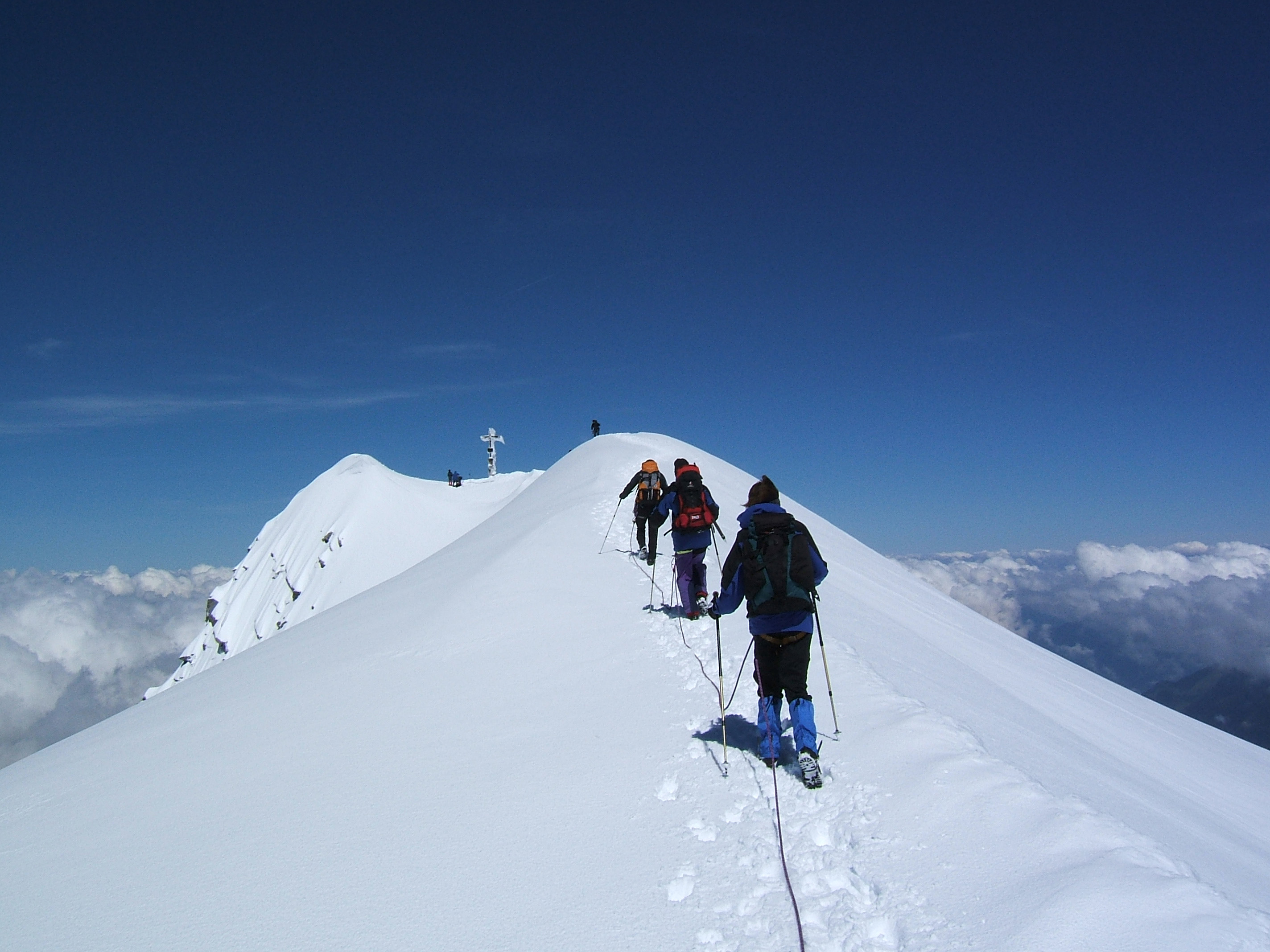
Figure 1: Rope team at a ridge nearing a summit. (Source: Wikimedia Commons)

In recent years, a variety of techniques have been developed to plan motions for a tethered mobile robot (Igarashi and Stilman, 2010; Teshnizi and Shell, 2014; Kim et al., 2014). A tether can be useful as a conduit for power or communication but the main motivating application for robotic tethers is in navigation of rovers in extreme terrain, where the tether can help provide physical security. Examples of robotic rovers equipped in this way include TRESSA (Huntsberger et al., 2007), Axel and DuAxel (Nesnas et al., 2012), vScout (Stenning et al., 2015), and TReX (McGarey et al., 2018), among others. Humans deal with extreme terrain too. A common practice among mountaineers, as a measure of protection against falling, is to form a group that can move together while the members are roped to one another. This forms what is referred to as a rope team (Gooding and Martin, 2014) (Fig. 1). From the perspective of motion planning, one might interpret a rope team as a practical scenario in which a tethered robot’s base is itself subject to motion. A prominent robotic example of comparable operation is DuAxel, where two Axel rovers are connected to a central module. DuAxel is designed to work as a mother-daughter ship, having one Axel remain stationary with the central module while the other explores the terrain. Indeed, enabling both rovers to be deployed simultaneously may benefit both agents and improve the versatility of the design.

One key to efficient solution of planning problems in finding a suitable representation, ideally one that expresses constraints and is amenable to adaptation and generalization to various requirements. Much like our earlier work (Teshnizi and Shell, 2014), we take advantage of the properties of reduced visibility graph (Latombe, 1991). Namely, we show certain characteristics of straight line motions enable us to find solutions to tethered pair problem with minimal book keeping. Unlike that work, however, the proofs proceed without needing to supply geometric or topological insight from the structure of configuration space (c-space). We do discuss, in Section 8, some of our understanding of the c-space of this problem.

The theory established in this work shows that we shall not be concerned with the intermediate state of the cable: as long as we can achieve a goal configuration that is permitted by the length of the available cable, one can provide a planner to execute the motions that will transform the initial cable configuration to its final configuration. This would be trivial if the constraints involved were purely topological or we considered only a single robot. But with a finite cable, what one robot uses is unavailable to the other, coupling their motions in space and time. On the basis of this theory, we introduce a tree data structure that represent different cable configurations up to homotopy. Each branch in the tree down to a certain node is a representation of the shortest path required for the tethered pair to arrive at that node’s cable configuration. We have implemented A^⋆ search to expand the search tree and find an optimal solution while keeping track of the cable’s configuration up to homotopy. Lastly, we detail how to turn paths produced by the planner into trajectories for the motions that also minimize a time cost.

2 Related Work

We are interested in what is perhaps the most natural motion planning question for a tethered pair of robots, namely finding paths to take a pair of tethered robots from some initial configuration to a goal one, never violating a bound on the tether’s length throughout the motion. Although motion planning for a single tethered robot has been extensively studied (Shnaps and Rimon, 2013; Teshnizi and Shell, 2014; Kim et al., 2014; Teshnizi and Shell, 2016a; McCammon and Hollinger, 2017; McGarey et al., 2017), the literature reports comparatively little work on motion planning problems involving pairs of robots tethered to one another.

A notable exception is that pairs of conjoined robots have been studied for purposes of object manipulation. Kim et al. (2013) studied object separation using a pair of robots connected by a cable. Though superficially similar to our problem, as it involves the motion of a mutually connected pair of robots, the separation problem imposes quite a different set of constraints to a shortest path planning problem. For object separation the solution is only required to satisfy a homotopy requirement, allowing the robots to choose any arbitrary goal in the workspace that can satisfy such constraint. Consequently, in that work, the two robots move to the boundaries of the workspace. (This assumption also helps distinguish between separating versus non-separating configurations elegantly and concisely.) As Kim et al. are addressing a problem where the goal is specified topologically and they are not concerned with a cable of finite length, several of the complications we tackle do not arise in their setting.

More recently, Kim and Shell (2018) demonstrated a physical multi-robot system in which robots can make or break tether connections dynamically; a planner exploits this capability to find ways in which a robot team can manipulate objects efficiently, either with single robots operating concurrently, or as coupled pairs, as called for by the particular problem instance. A part of that problem is combinatorial and the work uses a sampling-based method, the present work being distinguished from that work on both fronts.

Our own prior work on finding short paths for a pair of tethered robots (Teshnizi and Shell, 2016b), attempted to use the solution to a single robot problem as an algorithmic building block. That approach was devised primarily as a means to build intuition for the topology of the four dimensional configuration space; the algorithm outlined in that work is inadequate, being neither a solution to the complete problem nor one that always yields optimal paths. Toward the end of the paper, we will return to this matter of visualizing the c-space in light of the correct and complete algorithm that is in this paper.

3 Problem statement

Let $O=\{o_{1},o_{2},o_{3},\dots,o_{n}\}$ be a (possibly empty) set of pairwise disjoint polygonal obstacles with vertices (written $\operatorname{verts}(O)$) in $\mathbb{R}^{2}$, with boundary curves $\delta o_{1},\delta o_{2},$ $\dots,\delta o_{n}$, respectively. We will write $\mathscr{W}$ for the free space, so $\mathscr{W}=(\mathbb{R}^{2}\backslash\bigcup_{i=1}^{n}o_{i})\cup(\bigcup_{i=1}^{n}\delta o_{i})$. Further, let robots $a$ and $b$ be two unoriented points in $\mathscr{W}$ that are connected to one another via a cable of finite length. For conciseness, let $\mathbb{I}=[0,1]$ be the unit interval.

Definition 1 (trpmpp).

The tethered robot pair motion planning problem (trpmpp) is a tuple,
$(\mathscr{W},O,\mathbf{r_{a}},\mathbf{r_{b}},\mathbf{d_{a}},\mathbf{d_{b}},\ell,c_{0})$, wherein:

• $\mathscr{W}$ is the free space,

• $O$ is the set of obstacles,

• $\mathbf{r_{a}}\in\mathscr{W}$ is the initial position of $a$,

• $\mathbf{r_{b}}\in\mathscr{W}$ is the initial position of $b$,

• $\mathbf{d_{a}}\in\mathscr{W}$ is the goal or destination of $a$,

• $\mathbf{d_{b}}\in\mathscr{W}$ is the goal or destination of $b$,

• $\ell\in\mathbb{R}^{+}$ is the length of the tether,

• $c_{0}:\mathbb{I}\to\mathscr{W}$ is the initial arrangement of the cable in $\mathscr{W}$, where $c_{0}(0)=\mathbf{r_{a}}$, and $c_{0}(1)=\mathbf{r_{b}}$, and

  $$\mathfrak{L}\left[c_{0}(s)\right]\vcentcolon=\int_{\mathbb{I}}c_{0}(s)\mathop{ds}\leq\ell.$$

A solution to trpmpp $(\mathscr{W},O,\mathbf{r_{a}},\mathbf{r_{b}},\mathbf{d_{a}},\mathbf{d_{b}},\ell,c_{0})$ is a pair of paths $(\tau_{a},\tau_{b})$ in which:

• $\tau_{a}:\mathbb{I}\to\mathscr{W}$ where $\tau_{a}(0)=\mathbf{r_{a}}$ and $\tau_{a}(1)=\mathbf{d_{a}}$, and

• $\tau_{b}:\mathbb{I}\to\mathscr{W}$ where $\tau_{b}(0)=\mathbf{r_{b}}$ and $\tau_{b}(1)=\mathbf{d_{b}}$, and

• for $\tau_{a}$ and $\tau_{b}$, there exists a $\mathscr{W}$-feasible motion for an $\ell$-length cable, as formalized next.

Definition 2 ($\mathscr{W}$-feasible motion for an $\ell$-length cable).

In the closed subset of the plane $\mathscr{W}\subseteq\mathbb{R}^{2}$, for two paths $\tau_{a},\tau_{b}:\mathbb{I}\to\mathscr{W}$ and length $\ell\in\mathbb{R}^{+}$, a function $c:\mathbb{I}\times\mathbb{I}\to\mathscr{W}$ is called a $\mathscr{W}$-feasible motion for an $\ell$-length cable if and only if the following three conditions hold:

1. (The cable connects the robots)

   $$\forall s\in\mathbb{I}:c(s,0)=\tau_{a}(s)\textrm{ and }c(s,1)=\tau_{b}(s),$$

2. (Cable has bounded length)

   $$\forall s\in\mathbb{I}:\mathfrak{L}\left[c_{s}(x)\right]\leq\ell,\textrm{ where }c_{s}(x)\vcentcolon=c(s,x),$$

3. (Continuity) $c$ is continuous with respect to the induced topologies.

A visual example that serves as a quick summary of the preceding definitions appears in Fig. 2.

Definition 3 (Distance optimality).

A solution pair $(\tau^{\star}_{a},\tau^{\star}_{b})$ for trpmpp $(\mathscr{W},O,\mathbf{r_{a}},\mathbf{r_{b}},\mathbf{d_{a}},\mathbf{d_{b}},\ell,c_{0})$ is called distance optimal if all other solutions $(p,q)$ have

$$\max\left(\mathfrak{L}\left[\tau^{\star}_{a}\right],\mathfrak{L}\left[\tau^{\star}_{b}\right]\right)\leq\max\left(\mathfrak{L}\left[p\right],\mathfrak{L}\left[q\right]\right).$$

This particular optimality metric models minimum energy consumption between the two robots. We will present a method that finds a distance optimal solution to a trpmpp. In Section 6 we show that solutions under this distance metric can yield optimal solutions under a time-based criterion too.

4 The solution concept

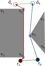
Figure 2: The green line segment is the initial cable configuration and the green dashed line segment is the final cable configuration. The arrows show the distance optimal path for each robot.

We prove, first, that it suffices to have robots $a$ and $b$ move on a straight line from one vertex to another in the reduced visibility graph (RVG). (Though our interest is in characterizing the solution set, this is potentially also good news in terms of the sensing technology needed for the robots to be able to execute optimal plans, cf. Tovar et al. (2007).) The following theorem and widely known corollary indicate that, for a single robot, the shortest path between two points in $\mathscr{W}$ is a concatenation of line segments that are edges of the RVG.

Theorem 4.1.

There exists a semi-free path between any two given points $\mathbf{p}$ and $\mathbf{q}$ if and only if there exists a simple polygonal line $T$ lying in $\mathscr{W}$ whose endpoints are $\mathbf{p}$ and $\mathbf{q}$, and such that $T$’s vertices are in $\operatorname{verts}(O)$. (Latombe, 1991; De Berg et al., 2008)

(a) The three paths used in the $\operatorname{cat}$ operator.

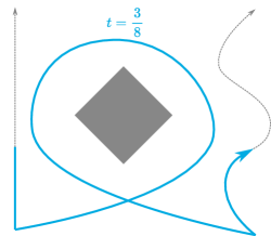
(b) Choosing a value for $t$ gives a curve.

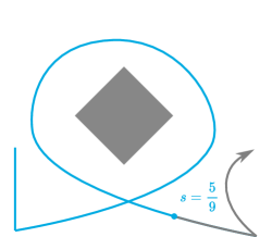
(c) Choosing a value for $s$ gives a point of the curve.

Figure 3: A visual explanation of how three paths are connected via the $\operatorname{cat}$ operator.

More useful for us the statement below which, though only stated informally by LaValle (1999), follows directly the previous result.

Corollary 1.

The shortest path for a robot from one point to another in a subset of $\mathbb{R}^{2}$ can be found by searching the shortest path roadmap or reduced visibility graph.

The list of RVG vertices $\pi_{a}=(v^{0}_{a},v^{1}_{a},\dots,v^{n-1}_{a},v^{n}_{a})$ connecting initial and destination positions, i.e., with $\mathbf{r_{a}}=v^{0}_{a}$ and $\mathbf{d_{a}}=v^{n}_{a}$ , is easily turned into a curve, $\tau_{a}(s)$, by joining line segments connecting $v^{i-1}_{a}$ to $v^{i}_{a}$ sequentially, head to tail, and parameterizing appropriately via $\mathbb{I}$. Hence, a pair of sequences of RVG vertices for the two robots, $(\pi_{a},\pi_{b})$, suffices to give a pair of paths $(\tau_{a},\tau_{b})$.

Although the preceding classical results hold for individual robots, when two robots are constrained such that the action of one limits the actions of the other (as in the case of a tether of finite length), then it is less clear that the discrete structure of the RVG encodes an optimal solution. One might conceive, in the two robot setting, one robot deviating from visibility edges in order to enable the other to move. A main result of the paper (Theorem 2), and the basis for the algorithm we present, establishes that no such deviations are necessary. Indeed, the RVG still suffices to find optimal solutions. More formally, let $\Pi_{a}$ be the set of all paths from $\mathbf{r_{a}}$ to $\mathbf{d_{a}}$ and let $\Pi_{b}$ be the set of all paths from $\mathbf{r_{b}}$ to $\mathbf{d_{b}}$ in the RVG. Proof of Theorem 2, the fact that $(\tau^{\star}_{a},\tau^{\star}_{b})\in\Pi_{a}\times\Pi_{b}$, is via several steps. The largest single intermediate step is in establishing Lemma 2, on the following page, but it requires a few definitions first.

To start, in what follows, we can think of an always taut tether. This is without loss of generality because: (1) tightening a tether is a continuous operation, so it preserves homotopy; (2) if the cable length constraint is satisfied for a taut tether, it must be for others as well. The reader should bear in mind that the taut tether is merely a special representative of the homotopy class of tethers. It is helpful to have an operator to give this representative:

Definition 4 (Tightening Operator).

Given a path $\alpha:\mathbb{I}\to\mathscr{W}$, we define the operator $\hat{\cdot}:(\mathbb{I}\to\mathscr{W})\to(\mathbb{I}\to\mathscr{W})$ such that $\hat{\alpha}$ is the (unique) shortest path in the homotopy class of $\alpha$.

Practically, the classical algorithm of Hershberger and Snoeyink (1994) is used to obtain the shortest path homotopic to a given path. The tightening operator will be used, in what follows, on paths and also on cable configurations. For the latter, the following definition helps.

Definition 5 (Connecting Paths via a Cable).

Given two paths $\tau_{1}:\mathbb{I}\to\mathscr{W}$ and $\tau_{2}:\mathbb{I}\to\mathscr{W}$, and a cable configuration $c:\mathbb{I}\to\mathscr{W}$, we define a function that concatenates $\tau_{1}$, $\tau_{2}$, and $c$. Let

$$\operatorname{cat}(s;t,\tau_{1},\tau_{2},c)\vcentcolon=\begin{cases}\tau_{1}(t-3st)&\quad 0\leq s\leq\frac{1}{3}\\ c(3(s-\frac{1}{3}))&\quad\frac{1}{3}<s<\frac{2}{3}\\ \tau_{2}(3(s-\frac{2}{3})t)&\quad\frac{2}{3}\leq s\\ \end{cases}\text{.}$$

Then, for any fixed $t\in\mathbb{I}$, argument $s\in\mathbb{I}$ parameterizes a new curve comprising those portions of $\tau_{1}$ and $\tau_{2}$ up to $t$ connected via $c$.

Since both $s$ and $t$ are curve parameters, the definition of $\operatorname{cat}$ can appear abstruse at first. Fig. 3 helps by illustrating how three given paths are joined via $\operatorname{cat}$ .

Definition 1, describing the planning problem, requires paths for which a feasible trajectory exists. The connection between paths and trajectories is, of course, a timing. Thus we need the following concept:

Definition 6 (Re-parameterization).

A re-parameterization is a monotonically increasing, continuous function $r:\mathbb{I}\to\mathbb{I}$ with $r(0)=0$ and $r(1)=1$. A pair $(r_{1},r_{2}$) is a re-parameterization pair if both functions, $r_{1}$ and $r_{2}$, are re-parameterizations.

With the preceding scaffolding, we can next give a definition that is valuable in helping to identify the existence of a feasible trajectory given paths. The notation $\circ$ is for function composition, i.e., $\tau_{1}\circ r_{1}(t)=\tau_{1}(r_{1}(t))$ and $\tau_{2}\circ r_{2}(t)=\tau_{2}(r_{2}(t))$.

Definition 7.

Given two paths $\tau_{1}:\mathbb{I}\to\mathscr{W}$ and $\tau_{2}:\mathbb{I}\to\mathscr{W}$, and a cable configuration $c:\mathbb{I}\to\mathscr{W}$, let

$$\mathbb{C}^{\star}(\tau_{1},\tau_{2},c)\vcentcolon=$$

$$\min_{\begin{subarray}{c}(r_{1},r_{2})~{}\text{over all}\\ \text{re-parameterization pairs}\end{subarray}}\left(\max_{t\in\mathbb{I}}\,\mathfrak{L}\left[{\widehat{\operatorname{cat}}(\cdot;t,\tau_{1}\circ r_{1},\tau_{2}\circ r_{2},c)}\right]\right).$$

Informally, $\mathbb{C}^{\star}$ gives the shortest cable that permits one to execute $\tau_{1}$ and $\tau_{2}$. The definition of $\mathbb{C}^{\star}$ resembles the Fréchet distance (Ewing, 1969). The key difference is that $\mathbb{C}^{\star}$ takes in a cable configuration $c$ and obtains the measure subject to the path connecting the two curves being constrained to a particular homotopy class. That homotopy class is prescribed via cable configuration $c$. (See also discussion in Section 8.)

The intuition which connects with the main result is that any solution $(\tau_{a},\tau_{b})$ to a given trpmpp must have a $\mathbb{C}^{\star}(\tau_{a},\tau_{b},c_{0})\leq\ell$. We would like to establish that any optimal solution to a given trpmpp can be related to some solution on the RVG (i.e., in $\Pi_{a}\times\Pi_{b}$) that, while being distance optimal, also abides by the conditions imposed by cable. Corollary 2 states this formally, but we need the following lemmas to get there.

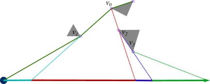
(a) A scenario illustrating the cable consumption function. Originally the cable is in contact with $v_{0}$ and $v_{1}$. As the robot travels towards its destination (to the right), it will release contact with $v_{1}$. It will then make contact with $v_{2}$ and $v_{3}$, respectively. The dotted lines represent places in which cable events occur.

(b) Length of consumed cabled as a function of curve parameter.

(c) Derivative of length of consumed cabled per change in curve parameter.

Figure 4: An illustrative example showing how, for a straight line motion, the cable consumption is a convex function. As the robot (in Fig. 4(a)) makes its way towards the destination, the cable will make or release contact with elements of $\operatorname{verts}(O)$. These events change the derivative of the consumed cable. Color coding of continuous motion helps show how the function’s pieces are separated by the occurrence of discrete cable events. Fig. 4(b) and 4(c) show the function and its derivative, respectively.

Lemma 1.

Path pair $(\tau_{a},\tau_{b})$ is a solution to a given trpmpp, iff $\mathbb{C}^{\star}(\tau_{a},\tau_{b},c_{0})\leq\ell$.

Proof.

For a contradiction assume $\mathbb{C}^{\star}(\tau_{a},\tau_{b},c_{0})>\ell$ and reach a contradiction with c-ii in Definition 2. ∎

The following lemma establishes an important fact about consumption of cable as the robots move on short paths. The result states that the consumption is a convex function, which leads to a practical way to verify that a pair of paths do not violate the limits imposed by the bounded cable, i.e., it suffices to check the lengths at the two end points.

Lemma 2.

Let $\widehat{\tau}_{a}$ and $\widehat{\tau}_{b}$, being the shortest paths in their respective homotopy classes, be the prescribed paths for robots $a$ and $b$. Then the length of the consumed cable is a convex function, if $\widehat{\tau}_{a}$ and $\widehat{\tau}_{b}$ use the same curve parameter.

Proof.

Because both $\widehat{\tau}_{a}$ and $\widehat{\tau}_{b}$ are the shortest paths in their respective homotopy classes, we can assert that they comprise sequences of pairwise connected straight line motions which lie on the RVG edges (following Corollary 1). Moreover, each straight line motion is of one of the following type:

• the motion is on the same edge as the cable and is [F]ollowing the cable, or

• the motion is on the same edge as the cable and is [L]eading the cable, or

• is any [O]ther straight line motion.

We will argue that the length of cable consumed as a robot moves along such trajectories is a convex function by showing that the gradient of the function is monotonically increasing. A technical difficulty with cable consumption is that it is a continuous but only piece-wise differentiable function. In circumstances where the derivative is undefined, we take the value of the derivative from the right. These circumstances arise when contacts between the cable and obstacles are made or broken. The cable consumption is a function of two curve parameters: so by derivative we are referring to the partials with respect to each parameter—one for each robot.

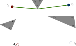
(a) The original configuration of the cable.

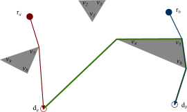
(b) The optimal solution to the given trpmpp which is found by searching the search tree.

Figure 5: An example scenario for which we illustrate part of the search tree in Fig. 6

When the robot is moving on an F (or L) segment the derivative is $-1$ (or $1$, respectively). For individual O segments the function might have multiple pieces. For each piece of each such segment, the pieces are regions where the points that the cable contacts are unchanged. Then, with a single robot moving, only the cable between the robot and the closest contact point contributes to the change in cable consumption. Writing the consumption as a function of the curve parameter and simply taking its derivative results in a monotonically increasing function whose value is in the $(-1,1)$ interval. When unwinding around an object the derivative is negative but increasing; when breaking contact, the radius to the closest object increases, and so does the derivative. When making or maintaining contact, the derivative is positive, but still increasing. It is, thus, always increasing. (Fig. 4 illustrates this fact using an example.)

Next, we argue that $\widehat{\tau}_{a}$ and $\widehat{\tau}_{b}$ have a specific structure: each trajectory is of the form $\textbf{F}^{*}\textbf{O}^{*}\textbf{L}^{*}$ (where we have used regular expression notation with Kleene stars). Showing the following suffices:

1. no O segment is followed by an F segment, and

2. no L segment is followed by an O segment, and

3. no L segment is followed by an F segment.

For proof of (a): Assume there exists a motion, $\widehat{\tau}_{1}$, in which segment $A$ of type O ending at vertex $v$ is followed by an F segment, starting at $v$. As we may assume the cable is always taut, we can assert that it lies on the shortest path to $v$. Thus, replacing $A$ with a segment/segments in which the robot follows the cable to arrive at $v$ yields a shorter path than $\widehat{\tau}_{1}$. This is a contradiction as $\widehat{\tau}_{1}$ is the shortest path in its homotopy class.

Similarly, proof of (b): Suppose there exists a motion, $\widehat{\tau}_{2}$, in which an L segment ending at vertex $v$ is followed by segment $B$ of type O starting at $v$ and ending at $v^{\prime}$. Given that the robot is leading the cable and that we may assume the cable is always taut, the cable lies on the shortest path from $v$ to $v^{\prime}$. Again, replacing $B$ with a segment/segments in which the robot follows the path of a taut cable to arrive at $v^{\prime}$ will be shorter than $\widehat{\tau}_{2}$. But then $\widehat{\tau}_{2}$ can’t have minimal length within its homotopy class.

The proof for the impossibility of (c) is as follows: Tautening such a cable leads to a shorter, pure F segment. The L segment provided excess length; and its removal reduces the distance along which the robots need to move. But this contradicts the fact that the paths are the shortest in their respective homotopy classes.

Taken together, this proves that $\widehat{\tau}_{a}$ and $\widehat{\tau}_{b}$ are of the form $\textbf{F}^{*}\textbf{O}^{*}\textbf{L}^{*}$. Hence, global monotonicity of the partial derivative of the cable consumption function holds if we can show that monotonicity is preserved between two consecutive O segments. To show no violation occurs at the transition between segments, monotonicity in a small open interval around the transition is sufficient. If the two O-segments, $g_{1}$ and $g_{2}$, are collinear, then they could be treated as a single segment and the prior argument for a single O-segment holds. Hence, there must be a ‘turn’ from segment $g_{1}$ to $g_{2}$. Both segments are on the RVG so that turn occurs at a vertex $v_{o}$ of some obstacle. Presume that we extend and continue along $g_{1}$ an extra $\epsilon>0$; then the derivative of the cable consumption continues to increase (as the single segment argument holds). Since $g_{2}$ is not along this little extension, it falls to one side. If that side is away from the cable-obstacle contact, then the additional motion away consumes extra cable, so the derivative only increases faster. Otherwise, when turning towards the contact, monotonicity may indeed fail. However, such a turn leads to a contradiction; two cases are possible: the obstacle to which $v_{o}$ belongs is on the inside of the turn, or it is on the outside. If it is on the inside, then the cable itself wraps around $v_{o}$, in which case $g_{2}$ is not an O segment (but an L one). If the obstacle is on the outside, then simply shaving off a small corner at the turn is feasible. But that is shorter, contradicting the supposition that $g_{1}$ and $g_{2}$ result from shortest motions in their homotopy class.

Hence monotonicity of the partial derivative of the cable consumption holds across the entire $\mathbb{I}$. Now consider the concurrent motion of both robots: we feed them the same curve parameter and the derivative of the cable consumption simply becomes the total derivative. Being the sum of two partials, each of which is monotone, gives a monotone function. Thus, the total cable consumption is a convex upward function of the curve parameter. ∎

The preceding does the heavy lifting for the proof of our theorem.

Theorem 4.2.

If $(\tau_{a},\tau_{b})$ is a solution for a given trpmpp, then $\exists(\tau^{VG}_{a},\tau^{VG}_{b})\in\Pi_{a}\times\Pi_{b}:\mathbb{C}^{\star}(\tau^{VG}_{a},\tau^{VG}_{b},c_{0})\leq\ell$.

Proof.

Let $\widehat{\tau}_{a}$ and $\widehat{\tau}_{b}$ be the shortest paths homotopic to $\tau_{a}$ and $\tau_{b}$, respectively. Hence, $(\widehat{\tau}_{a},\widehat{\tau}_{b})\in\Pi_{a}\times\Pi_{b}$ from Corollary 1. Then to prove this theorem it suffices to show that the following inequality holds:

$$\mathbb{C}^{\star}(\widehat{\tau}_{a},\widehat{\tau}_{b},c_{0})\leq\ell\text{.}$$

Since  $\hat{\cdot}$  is homotopy preserving, the following conditions hold:

$$\mathfrak{L}\left[{\widehat{\operatorname{cat}}(\cdot;0,\widehat{\tau}_{a},\widehat{\tau}_{b},c_{0})}\right]=\mathfrak{L}\left[{\widehat{\operatorname{cat}}(\cdot;0,\tau_{a},\tau_{b},c_{0})}\right]=\mathfrak{L}\left[\widehat{c}_{0}\right]\text{,}$$

$$\mathfrak{L}\left[{\widehat{\operatorname{cat}}(\cdot;1,\widehat{\tau}_{a},\widehat{\tau}_{b},c_{0})}\right]=\mathfrak{L}\left[{\widehat{\operatorname{cat}}(\cdot;1,\tau_{a},\tau_{b},c_{0})}\right]\text{.}$$

Moreover, because $(\tau_{a},\tau_{b})$ is a solution we have
$\mathfrak{L}\left[{\widehat{\operatorname{cat}}(\cdot;0,\widehat{\tau}_{a},\widehat{\tau}_{b},c_{0})}\right]\leq\ell$, and
$\mathfrak{L}\left[{\widehat{\operatorname{cat}}(\cdot;1,\widehat{\tau}_{a},\widehat{\tau}_{b},c_{0})}\right]\leq\ell$.

Following Lemma 2, feeding the same curve parameter to both $\widehat{\tau}_{a}$ and $\widehat{\tau}_{b}$, gives a convex upward cable consumption. Therefore,

$$\max_{t\in\mathbb{I}}\, \mathfrak{L}\left[{\widehat{\operatorname{cat}}(\cdot;t,\widehat{\tau}_{a},\widehat{\tau}_{b},c)}\right]=$$

$$\max_{t\in\{0,1\}}\,\mathfrak{L}\left[{\widehat{\operatorname{cat}}(\cdot;t,\widehat{\tau}_{a},\widehat{\tau}_{b},c)}\right]\leq\ell\text{.}$$

Because the above holds for the trivial identity re-parameterization, the minimum over the set of all re-parameterization pairs must be less than or equal to the above. This fact, when combined with Lemma 1, completes the proof. ∎

Corollary 2 (Distance Optimality).

Let $(\tau^{\star}_{a},\tau^{\star}_{b})$ be a distance optimal solution to a given trpmpp. Then the RVG also contains a distance optimal solution,
$(\tau^{\star VG}_{a},\tau^{\star VG}_{b})$.

Proof.

A pair $(\tau^{\star VG}_{a},\tau^{\star VG}_{b})\in\Pi_{a}\times\Pi_{b}$ is constructed from $(\tau^{\star}_{a},\tau^{\star}_{b})$. Simply take $(\tau^{\star VG}_{a},\tau^{\star VG}_{b})=(\widehat{\tau^{\star}_{a}},\widehat{\tau^{\star}_{b}})$ and observe the three following facts:

• $\widehat{\tau^{\star}_{a}}$ and $\widehat{\tau^{\star}_{b}}$ is on the RVG,

• the distance traveled along $\widehat{\tau^{\star}_{a}}$ and $\widehat{\tau^{\star}_{b}}$ for each robot is no worse following Corollary 1,

• $\mathbb{C}^{\star}(\widehat{\tau^{\star}_{a}},\widehat{\tau^{\star}_{b}},c_{0})\leq\ell$ following Theorem 4.2.

∎

5 The Efficient Planning Algorithm

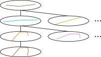
(a) A visual representation of the search tree, with vertices bearing labels that are iconic depictions of the cable configurations; see (b)–(d).

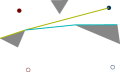
(b) Two of the configurations that can be achieved from the configuration stored in the root node.

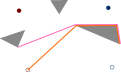
(c) Both cables shown here can be achieved from the cyan one in the previous snapshot. Orange is preferred as it reduces the distance traveled by robot $a$.

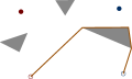
(d) The final configuration to arrive at the destination node.

Figure 6: A small portion of the search tree for the trpmpp in Fig. 5. The optimal solution to the given trpmpp in this figure can be obtained by traversing the node containing the brown cable configuration up to the root.

In this section we present an implementation of A^⋆ (Hart et al., 1968) to construct and explore the search tree for the solution to this problem. Consider a trpmpp with $(\mathscr{W},O,\mathbf{r_{a}},\mathbf{r_{b}},\mathbf{d_{a}},\mathbf{d_{b}},\ell,c_{0})$. The search tree’s nodes represent cable configurations. An edge between two nodes represents a motion for each robot along an RVG edge that abides by the cable requirements. To do so, we define a data-structure with the following fields:

• taut cable: a list of RVG vertices each of which is visible from the previous ones describing a valid cable configuration,

• cost: a pair of costs indicating the distance traveled by each robot to arrive at this cable configuration from their initial poses,

• a reference to a parent node.

Fig. 5 provides an example scenario, and Fig. 6 gives the structure of the search tree for this scenario. Using A^⋆ search, Algorithm 1 explores the search tree —which gives a structured representation to the set $\Pi_{a}\times\Pi_{b}$— for an optimal solution to a given trpmpp. Being a type of informed search, A^⋆ uses an estimated cost computed as the sum of a cost function and an heuristic function. The cost is calculated cumulatively with a constant time operation when creating/updating a node. When using an admissible heuristic function, we can safely terminate the search in a branch whose estimated cost is higher than the best solution found (Russell and Norvig, 2010). In Sec. 7.3 we examine the effect of different admissible heuristics on the efficiency of the algorithm.

1:  Search$(\mathscr{W},O,\mathbf{r_{a}},\mathbf{r_{b}},\mathbf{d_{a}},\mathbf{d_{b}},\ell,c_{0})$

2:  Build RVG, $g$, with vertices $\{\operatorname{verts}(O),\mathbf{r_{a}},\mathbf{r_{b}},\mathbf{d_{a}},\mathbf{d_{b}}\}$

3:  root $=$ Node($\widehat{c}_{0}$, $\varnothing$)

4:  priorityQ $=\{$ root $\}$

5:  while priorityQ is not empty do

6:     n = priorityQ.dequeue()

7:     if n.cable.first $=\mathbf{d_{a}}$ and n.cable.last $=\mathbf{d_{b}}$ then

8:        if $\mathfrak{L}\left[\text{n.cable}\right]\leq\ell$ then

9:           return  constructed path by following parent references from n up to the root

10:        else

11:           continue

12:        end if

13:     end if

14:     $V_{a}=g.$visibleVerts$($n.cable.first$)$

15:     $V_{b}=g.$visibleVerts$($n.cable.last$)$

16:     for all $(v_{a},v_{b})\in V_{a}\times V_{b}$ do

17:        $c_{1}=[v_{a}]+$ n.cable $+[v_{b}]$

18:        child $=$ Node($\widehat{c}_{1}$, n)

19:        priorityQ.enqueue(child)

20:     end for

21:  end while

Algorithm 1 A^⋆ over Cable Configurations

Given any node in the tree, we can obtain a pair of paths —one for each robot— that continuously transforms the original cable configuration to the configuration stored in the node. To do so, we can traverse the tree from the root down to the node. Start with $\pi_{a}$ and $\pi_{b}$ as two empty sequences. While traversing the tree down to the node, for each node we take the first and last element of the taut tether and append it to the end of $\pi_{a}$ and $\pi_{b}$, respectively. Notice that the sequences $\pi_{a}$ and $\pi_{b}$ will have equal cardinality. In fact, we see that the taut cable list at each vertex operates like a deque. Each robot, by making continuous motions in the plane, can modify the cable. The important qualitative changes to the cable are cable events: wherein an obstacle vertex is added or deleted. The physical property of the cable means that each robot’s motion can only push or pop at its respective end of the cable.

Theorem 5.1 (Soundness).

A pair of paths, $(\tau_{a},\tau_{b})$, generated by traversing the above mentioned search tree from the root to a leaf is a solution to the corresponding trpmpp, if the leaf contains a taut tether configuration whose end points are $\mathbf{d_{a}}$ and $\mathbf{d_{b}}$.

Proof.

The root contains the taut tether $\hat{c}_{0}$, which by definition has end points $\mathbf{r_{a}}$ and $\mathbf{r_{b}}$. Because the algorithm checks whether a leaf contains a taut tether configuration whose end points are $\mathbf{d_{a}}$ and $\mathbf{d_{b}}$ on line 7, the requirements $\tau_{a}(0)=\mathbf{r_{a}}$, $\tau_{a}(1)=\mathbf{d_{a}}$, $\tau_{a}(0)=\mathbf{r_{a}}$, and $\tau_{a}(1)=\mathbf{d_{a}}$ is satisfied. Using the result of Theorem 4.2, the check on line 8 ensures $(\tau_{a},\tau_{b})$ satisfies the final requirement for a solution. ∎

Theorem 5.2.

Algorithm 1 is complete.

Proof.

Completeness is shown by considering completeness of A^⋆ search, and Corollary 2 that indicates that the appropriate structure generated from the RVG is the solution space. ∎

6 From Paths to Trajectories

In Section 3 we defined a distance optimal solution. Solving a trpmpp only requires the existence of a $\mathscr{W}$-feasible motion for an $\ell$-length cable. This abstracts away details of time and allows us to consider a geometric problem, i.e., one on paths. But actually moving the robots requires trajectories. This last step is important to solve the problem we have laid out: we have proven the existence of some timing for the paths returned by the algorithm, but some timings (indeed many of them!) can violate the cable constraint during execution. Thus, next, we prescribe a suitable timing.

Informally, an execution for a tethered pair of robots is a function that maps a trpmpp solution (i.e., a pair of paths) to a pair of trajectories (as defined by Latombe (1991)), one for each robot. We assume robots $a$ and $b$ both have maximum speeds of $mv$ and that turning is instantaneous. For simplicity, we further assume that the robots can achieve speed $mv$ immediately.

For a given a pair of paths $(\tau_{a},\tau_{b})$, define

$$\qquad T=\max\left\{\frac{\mathfrak{L}\left[\tau_{a}\right]}{mv},\frac{\mathfrak{L}\left[\tau_{b}\right]}{mv}\right\}, \dagger$$ ()

that is, $T$ is the time which it takes for the robot that, moving at maximum speed throughout, arrives at its destination second. Then we construct trajectories $\Upsilon_{a}:[0,T]\to\mathscr{W}$ and $\Upsilon_{b}:[0,T]\to\mathscr{W}$ as follows

$$\quad\Upsilon_{a}(\lambda)=\tau_{a}\left(\frac{\lambda}{T}\right)\quad\text{ and }\quad\Upsilon_{b}(\lambda)=\tau_{b}\left(\frac{\lambda}{T}\right). \ddagger$$ ()

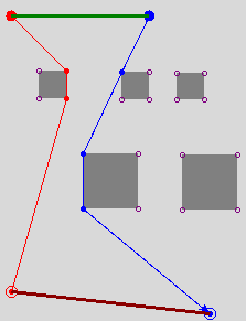
(a) $\ell=200$ and $\ell=300$

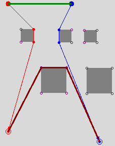
(b) $\ell=400$

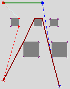
(c) $\ell=500$

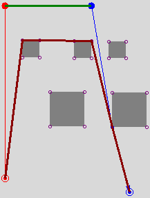
(d) $\ell=700$

Figure 7: Solving the same scenario with different cable length.

Note that by construction neither robot exceeds the maximum velocity.

Now, with notation for trajectories, the time index means we can define a temporal notion of optimality.

Definition 8 (Time optimality).

A pair of trajectories $(\Upsilon^{\star}_{a},\Upsilon^{\star}_{b})$ that are executions for a trpmpp solution is called time optimal if no other trajectories have both $a$ and $b$ arriving at $\mathbf{d_{a}}$ and $\mathbf{d_{b}}$ sooner than the later of the two under $\Upsilon^{\star}_{a}$ and $\Upsilon^{\star}_{b}$.

Leading to the following final claim:

Theorem 6.1.

Given a distance optimal solution $(\tau_{a},\tau_{b})$ returned by Algorithm 1, the pair of trajectories constructed by ($\dagger$ ‣ 6) and ($\ddagger$ ‣ 6) constitutes a time optimal execution.

Proof.

Algorithm 1 produces distance optimal solutions such that $(\tau_{a},\tau_{b})=(\widehat{\tau}_{a},\widehat{\tau}_{a})$. Then Lemma 2 provides that the trajectories $(t_{a},t_{b})$ abide by the cable constraints. The distance metric searches for minimum of the maximum distance traveled by either robots and the total time taken, given by ($\dagger$ ‣ 6), is the fastest the robots could travel that distance. ∎

7 Discussion of the Method

To demonstrate this algorithm, we implemented it in Python (v3). Our implementation makes heavy use of The CGAL Project (2020) for computational geometry algorithms, namely convex hull and triangulation methods. Fig. 8 shows a screenshot of the user interface.

7.1 Empirical Assessment of the Method: a Comparison

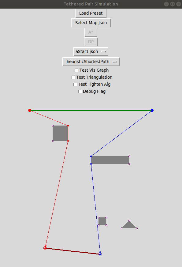
Figure 8: A screenshot of user interface of our implementation. The red and blue circle filled circles represent the robots. Obstacles are in grey. The initial and final configuration of the cable are shown in green and dark red. The prescribed path for each robot is shown with lines of the same color. The RVG vertices where for each robot is shown with small dots along the path.

Figure 9: The scenario used for comparison between Dynamic Programming and A^⋆ formulations.

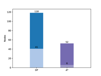
Figure 10: A comparison between the performance of Dynamic Programming vs. the A^⋆ formulation. In each bar, the light and dark color represent the number of expanded and generated search nodes for each algorithm. The bars are stacked as expanded nodes are a subset of the generated ones.

Our earlier workshop paper (Teshnizi and Shell, 2014) proposed a dynamic programming (DP) approach for motion planning for a tethered pair. The approach uses, as a sub-procedure, a planner for the motion of a single robot connected to a fixed base with a bounded tether. The method in that work does not rely on any specific single robot planner, as long as it can return as output the cost and the length of the tightened cable. As stated in that paper, the DP technique only solves instances of trpmpp of a particular form: it will only return motions of the robots that retain at least one contact point on the cable throughout the execution.  Hence, it is not a complete algorithm.

Meaningful comparison of Algorithm 1 and the DP approach requires that we select a problem for which the latter will return a solution. The scenario shown in Fig. 9 meets this criterion and it was the setting used for our empirical assessment. To remove the impact of implementation details on performance, we implemented the DP technique in Python using a specialized trpmpp planner setup to solve for a single robot.

Here, for a heuristic function, we use the straight line (Euclidean) distance (which we denote SLD) between the robots and their destinations. This can be computed in constant time. We measured the performance in terms of the number of search tree nodes expanded and generated as well as wall time. Table 1 and Fig. 10 present these metrics. It is obvious that A^⋆ formulation outperforms DP.

Table 1: Comparison of the performance between DP versus A^⋆ formulations on the scenario in Fig. 9.

Algorithm	Expanded	Generated	Wall Time ($\mathrm{s}$)
DP	41	118	4.52
A⋆	6	52	1.26

7.2 The Impact of Cable Length

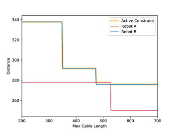
Figure 11: The distance traveled by each robot in optimal solution for different maximum cable lengths for scenario shown in Fig. 7. The constraint that the planner attempts to optimize is highlight for each cable length.

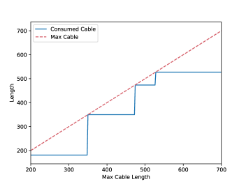
Figure 12: The length of the consumed cable in optimal solution for different maximum cable lengths for scenario shown in Fig. 7

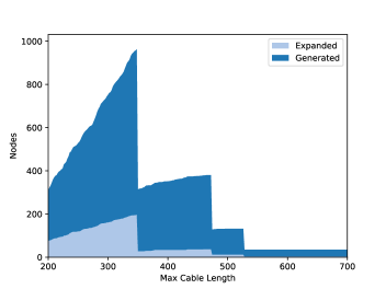
Figure 13: The number of expanded vs. generated nodes for different maximum cable lengths for scenario shown in Fig. 7.

The amount of the cable influences the search in two ways. To gain an understanding of the impact of cable length on the problem, we solved the sequence of planning instances depicted in Fig. 7. For each of these the environment is kept the same, so geometrical complexity is constant, only the maximum cable length is modified. Naturally, the objective values of the solutions decrease monotonically with increasing cable length. This can be seen in Fig. 11: as the length of the cable is increased, the planner minimizes the active constraint, which can be seen to switch from one robot to the other around $\ell=470$ and again at $\ell=525$. The steps are qualitative changes in solutions occurring as the tether becomes long enough to permit a new homotopy class of solutions. Observing Fig. 12 one sees that the steps happen as the length of the consumed cable in the optimal solution equals $\ell$ exactly.

Every solution for a cable of length $\ell$ is a solution for longer cables too. But if longer cables mean larger solutions spaces, they also mean larger search spaces. One might expect, therefore, that solving problems with longer cables would take more time. Fig. 13 shows the number of search nodes for cables ranging in length from $200$ to $700$. Observe that there is a steady increase with the algorithm exploring a subset of a search space which is growing, from $200$–$350$. But then the cable becomes long enough for the search to terminate much sooner. The pattern is repeated a few times. What happens is that the heuristic pulls the search towards parts of that space which, though promising, are not fruitful because the topological constraint will ultimately make them dead-ends. With a longer cable, branches that moved in the right direction but then turned out to be infeasible, now become feasible.

7.3 The Effect of Informed Search

The topology of the environment as well as the cable length affects both the number of expanded and generated nodes in the search. Making an appropriate choice of heuristic function for A^⋆ can help. In the previous sections, we reported results from the simple SLD heuristic. This heuristic is naïve, completely discarding topological and obstacle constraints, but still improves the efficiency of the search substantially. We established this fact via a comparison to a base-line. We implemented Uniform Cost Search (UCS) which yields an optimal output but without any forward estimates. Fig. 14 shows the impact of the heuristic information is significant.

More sophisticated heuristics, that consider more than simple Euclidean distance, can help reduce the search time further. Specifically, we considered two other heuristic functions, each being lesser relaxations of the problem:

• Shortest Path Distance (SPD) respects obstacles: it is the length of the shortest path from a robot’s position vertex to its destination. We compute this by running A^⋆ on the single (untethered) robot problem, itself using SLD.

• trpmpp Jr. respects obstacles and some topological constraints. It is computed by running a version of the problem instance at hand by but with a longer maximum cable, with SPD. (It is so named because it considers a diminished version of trpmpp.)

For trpmpp Jr., we sought to develop a heuristic that considers some aspects of the cable’s configuration. The results described in previous section show that searches with longer cables tend to be faster, so it is plausible that trpmpp Jr. could be computed quickly and provide high-quality information to guide the search for the original trpmpp. Based on those results, it uses a cable length multiplier, as a function of the number of vertices on the taut tether, to allow faster computation for more complex cable configurations. Notice, also, that SPD can be thought of as trpmpp Jr. but with $\ell=\infty$. Hence, trpmpp Jr. dominates SPD, which in turn dominates SLD.

As is apparent from Fig. 15, these heuristics do reduce the number of nodes expanded and generated by the search, but the improvements—at least in this scenario—are minuscule. Another important consideration is that, while SLD is a constant time operation, SPD and trpmpp Jr. usually require substantial computation. When we compare wall times, in Fig. 16, SPD offers some small improvement, whereas trpmpp Jr. has no discernible value. Both SPD and trpmpp Jr. involve searching relaxed problems and, in light of Valtorta’s Theorem (Valtorta, 1984), it is perhaps unsurprising that the total number of nodes are so similar (visible in Fig. 15).

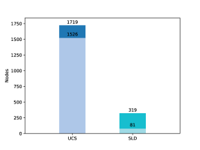
Figure 14: A comparison of number expanded and generated nodes between a Uniform Cost Search (UCS) vs. A^⋆ with Straight Line Distance (SLD) heuristic. The light and dark colors are stacked bars, representing expanded and generated nodes respectively.

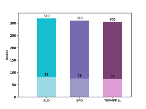
Figure 15: A comparison of number expanded and generated nodes between A^⋆ with three different heuristic functions: Straight Line Distance (SLD), Shortest Path Distance (SPD), and trpmpp Jr. The light and dark colors represent expanded and generated nodes.

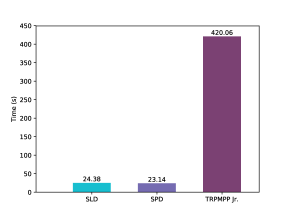
Figure 16: A comparison of computation wall time between A^⋆ with three different heuristic functions: Straight Line Distance (SLD), Shortest Path Distance (SPD), and trpmpp Jr.

8 Why is the tethered robot pair problem difficult?

Next we further consider the relationship of the present paper with respect to Teshnizi and Shell (2014); that paper defined and examined a useful way of decomposing the c-space of a single tethered robot. It constructed a tree structure that formed a skeleton that was related to an atlas representation of the c-space manifold.

Given the inputs to the single robot problem, one visualizes its c-space most easily by sketching the charts and showing where they touch (see Fig. 17). For the single tethered robot, this is (locally) a 2 dimensional object, and consequently easy to see. This structure allows for the convenient and simultaneous representation of two different pieces of data: the motion of the robot through space, and the homotopy class of the cable.

The single tethered robot problem is a special case of tethered pairs where one robot remains stationary: requiring only 2 degrees of freedom. For a general tethered pair, a comparable figure would require four dimensions, impeding easy visualization. In Fig. 18 we have moved the base of the tether slightly to the right to show the changes in the charts. The boundaries of these charts are 2D surfaces in a 4D space.

When there is some vertex where the cable makes contact, it is helpful to imagine two trees rooted at that point. Fig. 19 provides a view of this. From the perspective of our search tree, cable-obstacle contact that forms the common root is an element within the deque. (Recall the nodes of the search tree have cable configurations expressed as lists of vertices, which operate like a deque.) The subtrees on either side are represented by lists, via pushing and/or popping, that retain that element.

The robots share a total amount of cable, so as one either consumes or gives up cable, the depth of the tree or the circular regions circumscribing the outer limits of the other robot reduce or increase, respectively. One attractive aspect of this mental picture is how the cable describes a tree quite obviously: each time the cable wraps around an obstacle, some cable is consumed and it is as if it is anchored at that wrapping point. The recursive nature is clear because one obtains a new problem, similar to the previous one, but ‘smaller’ in the sense of available cable. This point of view was the main idea presented by Teshnizi and Shell (2016b).

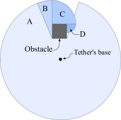
Figure 17: Some of the charts of the atlas representing the c-space of a tethered robot. $A$, $B$, $C$, and $D$ are four charts in the atlas. In the illustration, gray lines mark the chart boundaries.

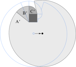
Figure 18: Moving the base of the tether leads to a changes in the boundaries of the charts. Here $A^{\prime}$, $B^{\prime}$, $C^{\prime}$ are the new charts. The charts prior to moving the base are illustrated in light blue for comparison.

If the robots start popping cable contacts out of the deque, moving up the tree (e.g., by following F segment after F segment) eventually the cable-obstacle contact that forms the common root is popped. At this point the node deque contains only the two robots and physically the robots must be directly visible to one another. They can then move and, stringing the tether between them, make a contact with another obstacle vertex. Doing so, leads back to a Fig. 19-like scenario. Hence, we can see that this top-level portion of c-space has many trees hanging like tendrils off of it. The top-level portion of c-space unlike the sort of charts made of pieces of spirals as depicted above, is truly 4D and comprises sub-regions where the pair of robots maintain line-of-sight. Consider that the reduced visibility graph, as a discrete structure, describes where tendrils can be found. But, further, the reduced visibility graph, as embedded in the plane, gives a way to think about the 4D chart if we restrict motions to the graph edges: within this space, the robots are either on the same vertex, or one edge away from each other. When restricted to paths on the visibility graph, within the 4D chart the robots must move on a sort of abstract boundary as they leapfrog and never get too far from one another, any deviation therefrom forming a tendril.

Previously, we said that our definition of $\mathbb{C}^{\star}$ resembles the classic Fréchet distance, but pointed out that it differs because $\mathbb{C}^{\star}$ respects the homotopy class of the paths being considered. Adopting the perspective of the c-space manifold, if $\tau_{1}$ and $\tau_{2}$ are curves not in $\mathscr{W}$, but instead in the 4D c-space, then $\mathbb{C}^{\star}$ becomes the Fréchet distance. Our algorithm operates on paths in the workspace $\mathscr{W}$, which one might think of as projections from the 4D configuration space. Hence, to recover enough information to compute the distance requires the cable configuration in addition to $\tau_{1}$ and $\tau_{2}$.

Prior work (such as our own (Teshnizi and Shell, 2014) and also others) has recognized the structure of the tree-like discrete skeletons that describe the atlas for a fixed tether point. Most would recognize that pushing and popping (via physical motions over critical events in terms of visibility) only occurs at the free end of the cable, so the data-structure is essentially a stack. So in summary: a 2D c-space gives a stack, a 4D c-space gives two stacks joined end-to-end, a deque. We are not aware of a more general realization that two robots give rise to a discrete structure mirroring a deque, nor that the case of the empty structure has special significance. One observation that is plain from this discrete data-structure point of view is that there can be multiple ways to arrive at the same deque contents. Indeed, this underscores the fact that the tethered pair case occurs on a manifold with cycles within it; cycles that are absent for an anchored tether. Hence, the tendrils are woven together and one can ‘pick them up’ to re-root from several places.

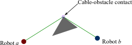
(a) The configuration of the robots and their cable.

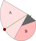
(b) The visibility charts for robot $a$.

(c) The visibility charts for robot $b$.

Figure 19: A snapshot of the conjoined atlases for a tethered robot pair after the first contact is made between the cable and an obstacle.

9 Conclusion

This work presents, to the best of our knowledge, a first algorithm for planning distance optimal motions for a pair of tethered robots. The finite cable length makes this problem different compared to work in the literature on tether pairs: prior work focuses on planning motions for a robot pair that need only consider topological constraints. In such cases, challenge becomes one of representing topological properties, via signatures or other techniques. In our case, it has turned out that the challenge was not the topological element of the problem, but rather the metric one that arises when considering a cable of bounded length. That is, determining if a path pair is a solution to a given trpmpp requires ensuring existence of a feasible trajectory for the cable of bounded length. The very question of whether solutions can be found in $\Pi_{a}\times\Pi_{b}$ (i.e., the RVG) is far more obvious when one robot’s motion only constrains the other’s topologically. It is not hard to see that timing (i.e., the robot’s motions relative to one another) becomes coupled and the problem involves dealing with some sort of coordination. Even glancing at the paper it is clear that greater care than is typical was needed to define what constituted a solution to a tethered pair motion planning problem so as to encode the finiteness of the cable.

Fortunately, shortest paths on an RVG help us avoid consideration of curve parameterizations: they have monotonically increasing derivative of cable consumption. Through this property, we can consider a much reduced set of solutions without losing completeness or optimality. Further, this provides an elegant representation of the search tree; one containing different cable configurations up to homotopy. We start by adding the initial configuration to the root node and iteratively create the configurations. Once we find a cable configuration that has the two robots’ destinations at its ends, only then we need to check whether that configuration is permitted but the length of the cable. Finally, using the properties of the solutions that our algorithm gives we are able to give an optimal execution. One that also minimizes the arrival time for the two robots.

The algorithm provided in this work enumerates all cable configurations that take the robots to their respective destination from least cost to most cost. We investigated the possibility of early termination in some branches in the search tree. However, our results have not yet provided adequate evidence that this added complexity improves performance consistently. Our immediate future work will explore the different ways to terminate the search in a branch of the search tree.

Acknowledgements

This work was supported, in part, by the National Science Foundation through awards IIS-1453652 and IIS-1849249. Fig. 1, whose author is Cactus26, is used without any further edits under Creative Commons Attribution-Share Alike 3.0 Unported license.

References

- De Berg et al. (2008) De Berg M, Cheong O, Van Kreveld M, Overmars M (2008) Computational geometry: Algorithms and applications, 3rd edn. Springer Berlin Heidelberg, Berlin, Heidelberg, DOI 10.1007/978-3-540-77974-2, arXiv:1011.1669v3
- Ewing (1969) Ewing G (1969) Calculus of Variations with Applications. W. W. Norton, URL https://books.google.com/books?id=oiUiAAAAMAAJ
- Gooding and Martin (2014) Gooding D, Martin JD (2014) Know The Ropes: Snow Climbing. Am Alp J URL http://publications.americanalpineclub.org/articles/13201212891/Know-The-Ropes-Snow-Climbing
- Hart et al. (1968) Hart PE, Nilsson NJ, Raphael B (1968) A Formal Basis for the Heuristic Determination of Minimum Cost Paths. IEEE Trans Syst Sci Cybern 4(2):100–107, DOI 10.1109/TSSC.1968.300136
- Hershberger and Snoeyink (1994) Hershberger J, Snoeyink J (1994) Computing minimum length paths of a given homotopy class. Comput Geom 4(2):63–97, DOI 10.1016/0925-7721(94)90010-8
- Huntsberger et al. (2007) Huntsberger T, Stroupe A, Aghazarian H, Garrett M, Younse P, Powell M (2007) TRESSA: Teamed robots for exploration and science on steep areas. J F Robot 24(11-12):1015–1031, DOI 10.1002/rob.20219
- Igarashi and Stilman (2010) Igarashi T, Stilman M (2010) Homotopic Path Planning on Manifolds for Cabled Mobile Robots. In: Algorithmic Found. Robot. IX, Springer, Berlin, Heidelberg, pp 1–18, DOI 10.1007/978-3-642-17452-0˙1
- Kim et al. (2013) Kim S, Bhattacharya S, Heidarsson HK, Sukhatme G, Kumar V (2013) A Topological Approach to Using Cables to Separate and Manipulate Sets of Objects. In: Robot. Sci. Syst.
- Kim et al. (2014) Kim S, Bhattacharya S, Kumar V (2014) Path planning for a tethered mobile robot. In: Proc. - IEEE Int. Conf. Robot. Autom., IEEE, pp 1132–1139, DOI 10.1109/ICRA.2014.6906996
- Kim and Shell (2018) Kim YH, Shell D (2018) Bound to help: cooperative manipulation of objects via compliant, unactuated tails. Autonomous Robots—Special Issue on Distributed Robotics: From Fundamentals to Applications 42:1563–1582
- Latombe (1991) Latombe JC (1991) Robot Motion Planning. Springer US, Boston, MA, DOI 10.1007/978-1-4615-4022-9
- LaValle (1999) LaValle SM (1999) Planning Algorithms. Cambridge University Press
- McCammon and Hollinger (2017) McCammon S, Hollinger GA (2017) Planning and executing optimal non-entangling paths for tethered underwater vehicles. In: 2017 IEEE Int. Conf. Robot. Autom., IEEE, pp 3040–3046, DOI 10.1109/ICRA.2017.7989349
- McGarey et al. (2017) McGarey P, MacTavish K, Pomerleau F, Barfoot TD (2017) TSLAM: Tethered simultaneous localization and mapping for mobile robots. Int J Rob Res 36(12):1363–1386, DOI 10.1177/0278364917732639
- McGarey et al. (2018) McGarey P, Yoon D, Tang T, Pomerleau F, Barfoot TD (2018) Developing and deploying a tethered robot to map extremely steep terrain. J F Robot 35(8):1327–1341, DOI 10.1002/rob.21813
- Nesnas et al. (2012) Nesnas IA, Matthews JB, Abad-Manterola P, Burdick JW, Edlund JA, Morrison JC, Peters RD, Tanner MM, Miyake RN, Solish BS, Anderson RC (2012) Axel and DuAxel rovers for the sustainable exploration of extreme terrains. J F Robot 29(4):663–685, DOI 10.1002/rob.21407
- Russell and Norvig (2010) Russell SJ, Norvig P (2010) Artificial intelligence : a modern approach, 3rd edn. Prentice Hall, DOI 10.1017/S0269888900007724
- Shnaps and Rimon (2013) Shnaps I, Rimon E (2013) Online Coverage by a Tethered Autonomous Mobile Robot in Planar Unknown Environments. In: Proc. Robot. Sci. Syst., Berlin, Germany
- Stenning et al. (2015) Stenning B, Bajin L, Robson C, Peretroukhin V, Osinski GR, Barfoot TD (2015) Towards Autonomous Mobile Robots for the Exploration of Steep Terrain. In: F. Serv. Robot. Results 9th Int. Conf., Springer, Cham, pp 33–47, DOI 10.1007/978-3-319-07488-7˙3
- Teshnizi and Shell (2014) Teshnizi RH, Shell DA (2014) Computing cell-based decompositions dynamically for planning motions of tethered robots. In: 2014 IEEE Int. Conf. Robot. Autom., IEEE, Hong Kong, China, pp 6130–6135, DOI 10.1109/ICRA.2014.6907762
- Teshnizi and Shell (2016a) Teshnizi RH, Shell DA (2016a) Planning motions for a planar robot attached to a stiff tether. In: 2016 IEEE Int. Conf. Robot. Autom., IEEE, vol 2016-June, pp 2759–2766, DOI 10.1109/ICRA.2016.7487438
- Teshnizi and Shell (2016b) Teshnizi RH, Shell DA (2016b) Some Progress Toward Tethered Pairs. In: ICRA Work. Emerg. Topol. Tech. Robot., Stockholm, Sweden
- The CGAL Project (2020) The CGAL Project (2020) CGAL User and Reference Manual, 5th edn. CGAL Editorial Board
- Tovar et al. (2007) Tovar B, Murrieta-Cid R, LaValle SM (2007) Distance-Optimal Navigation in an Unknown Environment Without Sensing Distances. IEEE Trans Robot 23(3):506–518, DOI 10.1109/TRO.2007.898962
- Valtorta (1984) Valtorta M (1984) A result on the computational complexity of heuristic estimates for the A algorithm. Information Sciences 34(1):47–59, DOI 10.1016/0020-0255(84)90009-4