Combination anti-coronavirus therapies based on nonlinear mathematical models

Abstract

Using nonlinear mathematical models and experimental data from laboratory and clinical studies, we have designed new combination therapies against COVID-19.

Currently there are no approved treatments for the SARS-CoV-2 infection. Moreover, scientists do not know any treatment that would consistently cure COVID-19 patients. This paper is an argument for combination therapies against COVID-19. We investigate a nonlinear dynamical system that describes the SARS-CoV-2 dynamics under the influence of immunological activity and therapy. Using the nonlinear mathematical model and experimental data from laboratory and clinical studies, we have designed new combination therapies against COVID-19. The therapies are based on antivirals in combination with other therapeutic approaches. The general therapeutic plan is the following: Gene therapy and/or Antivirals plus Immunotherapy and Anti-inflammatory drugs and/or drugs that control Cytokine Storms plus Cytotoxic therapies. We believe that these new therapies can improve patient outcomes.

I Introduction

Emerging viral diseases have caused significant global devastating pandemics, epidemics, and outbreaks (Smallpox, HIV, Polio, 1918 influenza, SARS-CoV, MERS-CoV, Ebola, and SARS-CoV-2).
Currently there are no approved treatments for any human coronavirus infection. Moreover, scientists do not know any treatment that would consistently cure COVID-19 patients. The world is facing a general catastrophe as people see the reality of alarming rises in infections, a building economic crisis, a shortage of ventilators, the lack of coronavirus testing, and many other disasters. The governments are desperate to find a solution. In some cases, they are even promoting unproven “remedies”. The novel coronavirus presents an unprecedented challenge for everybody, including the scientist: the speed at which the virus spreads means they must accelerate their research. We need a treatment that is 95$\%$ effective in order to safely open the countries and save the world from an economic catastrophe.
There is a wealth of literature dedicated to mathematical modeling of the virus-immune-system interaction. See, for example Ref1. There are many treatments in development. However, most of them have drawbacks Ref2.
This paper is an argument for combination therapies against COVID-19. We have shown before that combination therapies can be better than monotherapies. For instance, for some cancer tumors, the immunotherapies do not work at all Ref3; Ref4; Ref5. We have proposed to use a combination of therapies that could eradicate the cancer completely Ref3; Ref4; Ref5. In the present paper we will design new therapies based on antiviral agents in combination with other therapeutic approaches. These new therapies should improve patient outcomes.

II Growth models

There are several famous equations that have been used to describe cell population growth: exponential, Gompertz, logistic, and power-law equations Ref6.

In reference Ref7, a biophysical justification for the Gompertz’s equation was presented.

The deduction is based on the concept of entropy. The entropy definition used in Ref Ref7 is the well-known Boltzmann-Gibbs extensive entropy. Gonzalez et al. have used the new non-extensive entropy Ref8; Ref9; Ref10 in the derivation of a new very general growth model Ref6.

The exponential, logistic, Gompertz, and power laws are particular cases of the new equation. The new model has the potential to describe all the known and future experimental data Ref6.
The non-extensive parameter $\bm{q}$ Ref8; Ref9; Ref10; Ref11 plays an important role in the new model. Suppose we are studying virus population dynamics.

Different types of viral infections can possess different values of the non-extensive parameter $\bm{q}$.
Boltzmann-Gibbs statistics satisfactorily describes nature if the microscopic interactions are short-range and the effective microscopic memory is short-ranged, and the boundary conditions are nonfractal.
There is a large series of recently found natural systems that present anomalies that violate the standard Boltzmann-Gibbs method.
A non-extensive thermostatistics, which contains the Boltzmann-Gibbs as a particle case, was proposed in a series of papers Ref8; Ref9; Ref10; Ref11.
Nowadays, scientists have produced a large amount of successful applications of the new theory . These are mostly phenomena in complex systems.
The mentioned thermodynamic theory contains the non-extensive entropy:

$$S_{q}=k\frac{1-\sum_{i=1}^{w}p_{i}^{q}}{q-1},$$ (1)

where $\bm{k}$ is a positive constant, $\bm{w}$ is the total number of possibilities of the system,

$$\sum_{i=1}^{w}p_{i}=1,\hskip 14.22636ptq\in\mathbb{R},$$ (2)

This expression recovers the Boltzmann-Gibbs entropy, $\bm{S_{1}=-k\sum_{i=1}^{w}p_{i}\ln p_{i}}$, in the limit $\bm{q}\rightarrow 1$. Parameter $\bm{q}$ characterizes the degree of non-extensivity of the system.
This can be seen in the following rule:

$$S_{q}(A+B)/k=\left[S_{q}(A)/k\right]+\left[S_{q}(B)/k\right]+(1-q)\left[S_{q}(A)/k\right]\left[S_{q}(B)/k\right],$$ (3)

where $\bm{A}$ and $\bm{B}$ are two independent systems in the sense that $\bm{P_{i,j}(A+B)=P_{i}(A)P_{j}(B)}$. We could say that parameter $\bm{(1–q)}$ characterizes the complexity of the system.
The case $\bm{1-q\geq 0}$ implies that the system is resilient.
For example, this condition indicates that the virus infection will lead to a drug-resistant disease. In particular, this disease can become resistant to the attack of the immune system and conventional therapy.

The new generalized equation for population growth is the following

$$\frac{dX}{dt}=\frac{kX_{\infty}}{q-1}\left[1-\left(\frac{X}{X_{\infty}}\right)^{q}-\left(1-\frac{X}{X_{\infty}}\right)^{q}\right],$$ (4)

where $\bm{X(t)}$ is the growing population, $k$ is certain free parameter, and $\bm{X_{\infty}}$ is the asymptotic value of $\bm{X(t)}$ when $\bm{t\rightarrow\infty}$.
We have already remarked that this is a very general model that contains most known growth models Ref6.

Now, we will show that this model is universal in the sense discussed in Ref. Ref12; Ref13 and includes many others classes of models as particulars cases. Ref13_1
For early stages of the infection, (4) can be written in the following form Ref13_1

$$\frac{dX}{dt}=\alpha_{q}\left(\frac{X}{X_{\infty}(q)}\right)^{q}\left[1-\left(\frac{X}{X_{\infty}(q)}\right)^{1-q}\right],$$ (4a)

where $$\bm{\alpha_{q}=\frac{kqX_{\infty}(q)}{1-q}} \bm{X_{\infty}(q)=q^{\frac{1}{q-1}}X_{\infty}}$$, .
An analytical solution to equation (4a) can be expressed as

$$\left(\frac{X}{X_{\infty}(q)}\right)^{1-q}=1-\left[1-\left(\frac{X_{0}}{X_{\infty}(q)}\right)^{1-q}\right]e^{-qkt}$$ (4b)

where $$\bm{X_{0}} \bm{X(t=0)=X_{0}}$$ is the initial condition so that .
We can re-write solution (4b) as

$$r(\tau)=1-e^{-q\tau}$$ (4c)

where $$\bm{r=\left(\frac{X}{X_{\infty}(q)}\right)^{1-q}} \bm{\tau=kt-\ln(1-r_{0})^{1/q}}$$ and .
This calculation shows that our model represents a universal growth law Ref12; Ref13; Ref13_1.
So even this general class of growth laws are a particular case of equation (4).

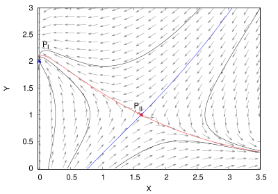
Figure 1: Phase space representation of the dynamics of the dynamical system (5) , (6). In this case, the fixed point $\mathbf{P_{I}}$ is a stable node, the point $\mathbf{P_{II}}$ is a saddle, and the point where $\mathbf{X\approx X_{\infty}}$ is a stable node (not shown). The blue line is the stable manifold of the saddle point $\mathbf{P_{II}}$. And the red line is the unstable manifold of the mentioned saddle point. The blue line is a global separatrix of the dynamics. All initial conditions that are on the “left” of the blue line will lead to a phase trajectory that tends to a point where $\mathbf{X=0}$. All initial conditions that are on the “right” of the separatrix will lead to a phase trajectory that tends to the point where $\mathbf{X\approx X_{\infty}}$. This picture occurs when $\mathbf{q>1}$ , $\mathbf{bV>af}$.

III The model

In the present paper, we will investigate the following dynamical system

$$\frac{dX}{dt} =\frac{kX_{\infty}}{q-1}\left[1-\left(\frac{X}{X_{\infty}}\right)^{q}-\left(1-\frac{X}{X_{\infty}}\right)^{q}\right]-bXY-c_{1}(t)X,$$ (5)

$$\frac{dY}{dt} =d(X-eX^{2})Y-fY+V-c_{2}(t)Y,$$ (6)

where $\bm{X}$ denotes the virus population and $\bm{Y}$ denotes the population of lymphocytes. Equation (5) describes the reproduction of the virus. The virus is killed when it meets agents of the immune system (term $\bm{-bXY}$).

The reproduction of the agents of the immune system is described by the term $\bm{d(X-eX^{2})}$, where initially the presence of the virus stimulates the reproduction of $\bm{Y(t)}$. When virus load is very large, the person is so sick that the reproduction of $\bm{Y(t)}$ is inhibited. The term $\bm{-fY}$ corresponds to the natural death of lymphocytes. The term $\bm{V}$ represents an external flow of lymphocytes.

The term $\bm{-c_{1}(t)X}$ stands for virus-killing process due to different therapies. The term $\bm{-c_{2}(t)Y}$ shows that therapies can also affect other normal cells (including the immune system).

The system (5) and (6) is inspired by models of the immune system developed in references Ref14 and Ref15. However, instead of the exponential growth assumed in Ref14; Ref15, we are using our growth model given by Eq. (4).

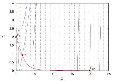
Figure 2: This situation is topologically equivalent to that shown in Fig. (1) However, now we can see the fixed point where $\mathbf{X\approx X_{\infty}}$. (Far right).

IV Investigation of the model

First, we will consider the case where $\bm{q>1}$, $\bm{X_{\infty}e>>1}$, $\bm{c_{1}(t)=0}$,$\bm{c_{2}(t)=0}$ .
Let us define $\bm{a=\frac{qk}{q-1}}$. The dynamical system (5)-(6) can have, in principle, four fixed points

$$P_{I}=(X_{1},Y_{1})=(0,\frac{V}{f})$$ (7)

$$P_{II}=(X_{2},Y_{2}),$$ (8)

where $\bm{\frac{1}{2e}<X_{2}<X_{\infty}}$, $Y_{2}=\frac{a}{b}$,

$$P_{III}=(X_{3},Y_{3}),$$ (9)

where $\bm{0<X_{3}<\frac{1}{2e}}$, $\bm{Y_{3}=\frac{a}{b}}$,

$$P_{IV}=(X_{4},Y_{4}),$$ (10)

where $\bm{X_{4}=X_{\infty}}$,
The conditions for the existence of points $\bm{P_{II}}$ and $\bm{P_{III}}$ are the following inequalities

$$\frac{1}{4e^{2}}-h >0,$$ (11)

$$h>0,$$ (12)

where $\bm{h=\left(f\frac{a}{b}-V\right)\frac{b}{ead}}$
The eigenvalues of the Jacobian matrix corresponding to the fixed point $\bm{P_{I}}$ are

$$\lambda_{1}^{(I)} =a-\frac{bV}{f},$$ (13)

$$\lambda_{2}^{(I)} =-f.$$ (14)

If $\bm{af<Vb}$, the fixed point $\bm{P_{I}}$ is a stable node and the fixed point $\bm{P_{II}}$ is a saddle (See figures (1) -(2)) . If $\bm{af>Vb}$, and $\bm{h-\frac{1}{4e^{2}}<0}$, then the four fixed points exist and are non-negative. Both fixed points $\bm{P_{I}}$ and $\bm{P_{II}}$ are now saddles. Between these two points, there is the point $\bm{P_{III}}$, which is stable (See Fig. (3) and Fig.(4))).

If $\bm{af>Vb}$, and $\bm{h-\frac{1}{4e^{2}}>0}$, then there are only two fixed points: point $\bm{P_{I}}$ which is now unstable and point $\bm{P_{IV}}$, which is stable. As a result, most trajectories tend to point $\bm{P_{IV}}$ (with maximum virus population) . This is not a very favorable situation for the patient. (See Fig. (5))

In the neighborhood of point $\bm{P_{II}}$, the separatrix of the saddle can be approximated by the straight line

$$Y=-\left(\frac{\lambda_{2}^{(II)}}{bX_{2}}\right)X+\frac{a+\lambda_{2}^{II}}{b}$$ (15)

Any point corresponding to initial conditions of the Cauchy problem on the right of the separatrix leads to a dynamics where the trajectory approaches the point of maximum virus load (point $\bm{P_{IV}}$).
On the other hand, if the initial conditions correspond to a point located on the left of the separatrix, the system will evolve to a stable fixed point.
Using (15), we can calculate the threshold or critical virus population that would lead to a dynamics approaching point $\bm{P_{IV}}$:

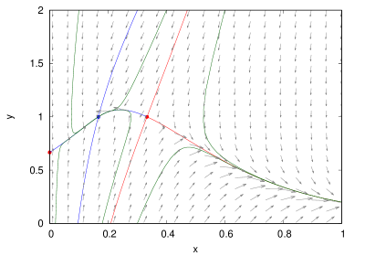
Figure 3: Phase space representation of the dynamics of system (5) ,(6) . In this case, the fixed point $\mathbf{P_{I}}$ is unstable, the fixed point $\mathbf{P_{II}}$ is still a saddle. Now there is a new fixed point $\mathbf{P_{III}}$ that is a stable node (for which $\mathbf{X>0}$). Now the separatrix is represented with a red line. All the phase trajectories that are on the “left” of the separatrix are approaching the point $\mathbf{P_{III}}$ (where $\mathbf{X>0}$). All the phase trajectories that are on the “right” of the separatrix are approaching the fixed point where $\mathbf{X\approx X_{\infty}}$. Note that there are trajectories for which $\mathbf{X(t)}$ is monotonically increasing from a small value until it reaches its maximum (Point $\mathbf{P_{III}}$ ). There are other trajectories for which $\mathbf{X(t)}$ reaches a maximum, and, later, it decreases until it enters the point $\mathbf{P_{III}}$ . Conditions $\mathbf{bV<af}$ and $\mathbf{h-\frac{1}{4e^{2}}<0}$ are satisfied.

$$X_{crit}=\left(1+\frac{a}{\lambda_{2}^{(II)}}\right)X_{2}.$$ (16)

When $\bm{X_{\infty}}$ is small, the outcome can be very favorable.
For instance, when

$$X_{\infty}<\frac{11}{6e}+\frac{2f}{3d},$$ (17)

all the phase trajectories tend to the fixed point $\bm{P_{I}(X=0)}$.
We can also apply the isocline method in order to further investigate the system. A careful analysis of the behavior of the phase trajectories allows us to conclude that the condition

$$d>4ef,$$ (18)

is favorable for the patient. This is a sufficient condition to avoid an uncontrollable rise of the virus population leading to the point $\bm{P_{IV}}$.
In many cases, it is convenient to re-write the system (5) -(6) as one equation where the only unknown is $\bm{X(t)}$,

$$\frac{d^{2}X}{dt^{2}}+\left[f-d(X-eX^{2})\right]\frac{dX}{dt}-\frac{1}{X}\left(\frac{dX}{dt}\right)^{2}=-\frac{dU(X)}{dX}$$ (19)

In general, it is useful to discuss the dynamics of virus population as a general equation of the following type

$$\frac{d^{2}X}{dt^{2}}+F_{dis}\left(X,\frac{dX}{dt}\right)=-\frac{dU}{dX}$$ (20)

See Refs Ref16 for a simple explanation. Equation (20) is equivalent to a Newton’s equation for a “fictitious” particle moving in the potential $\bm{U(X)}$ under the action of nonlinear damping.

The potential $\bm{U(X)}$ can have minima and maxima. So we can conceive the situation where the “fictitious” particle is trapped inside a potential well. The particle needs to jump over a barrier for the virus population to continue increasing. Studying the relative heights of the barriers, we get the condition

$$9e(Vb-af)+2ad>0,$$ (21)

when this condition is satisfied, the “right” barrier of the potential well is higher than the “left” barrier. This case is more favorable for the patient.
A careful analysis shows that the condition

$$2d>9ef,$$ (22)

is very favorable for the patient.
The general meaning of conditions (18), (21) and (22) is that the comparison between the values of $\bm{d}$ and the product $\bm{ef}$ can decide the outcome.
Let us analyze now the case $\bm{q\leq 1}$. When

$$q\leq 1,$$ (23a)

the point $$\bm{P_{I}}$$ will be always unstable. This means that it is almost impossible to reduce the virus population to zero. This finding will play a very important part in the design of new therapies.

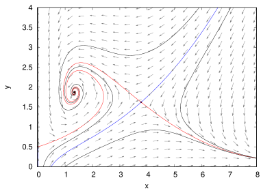
Figure 4: This dynamics is similar to that shown in Fig. (3). However, here the fixed point $\mathbf{P_{III}}$ is a stable focus.

Let us discuss time-dependent therapy against COVID-19.
Let us consider the dynamical system (5)-(6) with time-dependent therapy
$\mathbf{c_{1}(t)}$ and $\mathbf{c_{2}(t)}=\epsilon\,\mathbf{c_{1}(t)}$ where $\mathbf{\epsilon<1}$.
Using ideas from Ref6, we can obtain the following result. If $\mathbf{q<1}$, it is very difficult to cure the virus disease. If we have a target decay for the virus population $\mathbf{X(t)}$ , then $\mathbf{c_{1}(t)}$ must behave as

$$c_{1}(t)=\left[\frac{kX_{\infty}^{1-q}}{1-q}\right]\left(\frac{1}{X(t)^{1-q}}\right)$$ (23b)

For instance, if we require the virus population to be reduced following a power law, say $\mathbf{X(t)\approx\alpha/t^{\gamma}}$ , then the therapy must behave as $\mathbf{c_{1}(t)}=t^{\gamma(1-q)}$. The exponent gamma represents the rate of decay of the virus population.
We have designed therapies using the following late-intensification schedules:

$$c_{1}(t)=c_{0}\ln(e+\delta t)\,\,\text{ and}$$ (23c)

$$\,\,\,c_{1}(t)=c_{0}\left[1+\delta t\right]^{\gamma(1-q)}$$ (23d)

where $\mathbf{c(t)=c_{0}}$ is a well-known constant-dose treatment taken by a patient for several days. (See Ref. Ref4). Our logarithmic late-intensification schedule has been very successful (See Ref5 and references quoted there in). The traditional therapy is changed only slightly.
However, the results are spectacular.

V Monotherapies

When $\bm{q>1}$, the parameters of the system and the initial conditions play an important role in the outcome. The virus-host interaction is decisive. There are situations where the immune system by itself can reduce the virus population to zero. Under other circumstances, the virus population will increase to numbers that can threaten the patients survival. If we apply conventional antiviral therapies with $\bm{c(t)=c_{0}}$ in the system (5) and (6) (where $\bm{c_{0}}$ is a constant), for $\bm{q>1}$, the cure can be accelerated Ref6.
If $\bm{q\leq 1}$, then for any value of $\bm{c_{0}}$, the virus population is never reduced to zero. The fixed point $\bm{P_{I}}$ is always unstable.
The medical significance of this result can be expressed employing this statement: when $\mathbf{q\leq 1}$ the disease is resistant to the immune response and the action of conventional therapy.

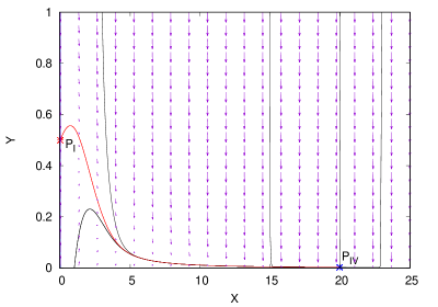
Figure 5: In this case, the fixed points $\mathbf{P_{II}}$ and $\mathbf{P_{III}}$ disappear. Point $\mathbf{P_{I}}$ is unstable. All the phase trajectories tend to the point $\mathbf{P_{IV}}$ , where $\mathbf{X\approx X_{\infty}}$. Conditions $\mathbf{af>Vb}$ and $\mathbf{h-\frac{1}{4e^{2}}>0}$ are satisfied.

VI Combination therapies

Our analysis shows that for $\bm{q\leq 1}$, the virus can develop resistance both against the attack of the immune system and all conventional monotherapies with constant doses of the medication. All this investigation leads to combination therapies.
First, we have to use therapies that change the parameters in such a way that fixed point $\bm{P_{I}}$ becomes asymptotically stable (a stable node). Then we need to apply therapies that will help the phase trajectory to go to the point $\bm{P_{I}}$. The condition $\bm{q>1}$ should be completed with the stability of fixed point $\bm{P_{I}}$:

$$bV>\frac{qkf}{q-1},$$ (23e)

and complemented with condition (18).
This means that immuno-therapy is also very important for the development of antiviral therapies.
This work can guide physicians to rationally design new drugs or a combination of already existing drugs for the development of antiviral therapies.

Condition (23e) shows that the killing ability of the immune system and the external flow of lymphocytes should be stronger than the virus replication and the natural death of immune system agents.

Additionally, condition (18) says that the reproduction of the lymphocytes should be stronger than the inhibition of the immune system due to the general health weaknesses created by the disease.

The perfect strategy is to use a therapy that can change $\bm{q}$ so that the fixed $\bm{P_{I}}$ can be, in principle, stable. Of course, this does not guarantee that the point $\bm{P_{I}}$ is stable.

The condition $\bm{q>1}$ is a necessary condition for the stability of point $\bm{P_{I}}$. However, it is not a sufficient condition.

Later we need another therapy that will change the other parameters (see section 3) so that the fixed point $\bm{P_{I}}$ is actually asymptotically stable. This step is probably satisfied with an immuno-therapy.

Finally, we need a treatment $\bm{c(t)}$ that definitely kills the virus, leading the phase trajectory to the fixed point. The ideal candidate for the first task could be a gene-targeted therapy. On the other hand, we believe there are antivirals that can be utilized in order to accomplish this goal.

VII Some biophysical analysis

Drug repurposing for SARS-CoV-2 is very important for our world. It can represent an effective drug discovery strategy from existing drugs. It could shorten the time and reduce the cost compared to de novo drug discovery Ref43.

Phylogenetic analysis of 15 HCoV whole genomes reveal that SARS-CoV-2 shares the highest nucleotide sequence identity with SARS-CoV Ref43.

A molecular docking study has been published by Abdo Elfiky Ref44.

The results show the effectiveness of Ribavirin, Remdesivir, Sofobuvir, Galidesivir, and Tenofovir as potent drugs against SARS-CoV-2 since they tightly bind to its RdRp. Additional findings suggest guanosine derivative (IDX-184), Sefosbuvir, and YAK as top seeds for antiviral treatments with high potential to fight SARS-CoV-2 strain specifically.

VIII Real experiments and clinical studies

We have reviewed the medical literature on COVID-19 treatments. There is experimental evidence supporting combination therapies Ref17; Ref18; Ref19; Ref20; Ref21; Ref22; Ref23; Ref24; Ref25; Ref26; Ref27; Ref28; Ref29; Ref30; Ref31; Ref32; Ref33; Ref34; Ref35; Ref36; Ref37; Ref38; Ref39; Ref40; Ref41; Ref42; Ref43; Ref44; Ref44; Ref45; Ref46; Ref47; Ref48; Ref49; Ref50; Ref51; Ref52; Ref53 However, medical practice has been concentrated mostly on monotherapies. Ref17; Ref18; Ref19; Ref20; Ref21; Ref22; Ref23; Ref24; Ref25; Ref26; Ref27; Ref28; Ref29; Ref30; Ref31; Ref32; Ref33; Ref34; Ref35; Ref36; Ref37; Ref38; Ref39; Ref40; Ref41; Ref42; Ref43; Ref44; Ref44; Ref45; Ref46; Ref47; Ref48; Ref49; Ref50; Ref51; Ref52; Ref53
Even when combination therapies have been used, in many cases, the combinations have not been optimized. We believe we can improve the treatment outcomes using our results.
Combination of antivirals is the most common therapeutic set. Ref17; Ref18; Ref19; Ref20; Ref21; Ref22; Ref23; Ref24; Ref25; Ref26; Ref27; Ref28; Ref29; Ref30; Ref31; Ref32; Ref33; Ref34; Ref35; Ref36; Ref37; Ref38; Ref39; Ref40; Ref41; Ref42; Ref43; Ref44; Ref44; Ref45; Ref46; Ref47; Ref48; Ref49; Ref50; Ref51; Ref52; Ref53 In many cases, the used antivirals were previously developed for other viruses (e.g. SARS, MERS, Ebola, Flu, and HIV). Ref17; Ref18; Ref19; Ref20; Ref21; Ref22; Ref23; Ref24; Ref25; Ref26; Ref27; Ref28; Ref29; Ref30; Ref31; Ref32; Ref33; Ref34; Ref35; Ref36; Ref37; Ref38; Ref39; Ref40; Ref41; Ref42; Ref43; Ref44; Ref44; Ref45; Ref46; Ref47; Ref48; Ref49; Ref50; Ref51; Ref52; Ref53
We present a summary of the studies about COVID-19 treatments.
Therapy 1: Lopinavir + Ritonavir (Antivirals against HIV) + Oseltamivir (Flu) Lopinavir/Vitanovir are approved protease inhibitors for HIV.
Results: There is some scientific evidence that this combination can work Ref17; Ref51; Ref52
Inconsistent results in some completed clinical trials.

Therapy 2: Antiflu Arbidol + Anti-HIV antiviral Darunavir.
Results: There is some scientific evidence that this combinations can help. Ref17; Ref51

Therapy 3: Lopinavir/Ritonavir + Ribavirin.
This is an anti-HIV therapy used in SARS.
Results: There is some scientific evidence that this combination could work Ref18.

Therapy 4: Remdesivir + Lopinavir/Ritonavir + Interferon beta.
Remdesivir interferes with virus RNA polymerases to inhibit virus replication, and was used for Ebola virus outbreak.
Results: The combination is being tested for MERS. There is some scientific evidence that this combination could work for other coronaviruses Ref18

Therapy 5: Cloroquine, Hydroxycloroquine.
This is an antimalarial drug.
Results: Inconsistent results in completed clinical trials Ref2; Ref20; Ref21; Ref25; Ref26; Ref35, and Ref38.

Therapy 6: Hydrocloroquine + antibiotic azithromycin.
Results: Dedier Raoolt and coworkers published results of a completed clinical trial that “proved” efficacy Ref20. However, nowadays, this therapy is considered controversial.

Therapy 7: Convalescent plasma.
Convalescent plasma from cured patients provides protective antibodies against
SARS-CoV-2.
Results: Proven efficacy Ref23; Ref27; Ref28; Ref29; Ref30; Ref31; Ref32; Ref52

Therapy 8: “Natural killer” cell therapy.
Natural killer cell therapy can elicit rapid and robust effects against viral infections through direct cytotoxicity and immunomodulatory capability.Ref52
Results: Being tested in clinical trials Ref52; Ref30, and Ref37.

Therapy 9: EIDD-2801.
This is an antiviral.
EIDD-2801 is incorporated during RNA synthesis and then drives mutagenesis, thus inhibi-ting viral replication Ref52.
Results: Being tested in clinical trials Ref36; Ref37; Ref52.

Therapy 10: Remdesivir.
This is an antiviral that interferes with virus RNA polymerases to inhibit virus replication.
Results: Approved by FDA Inconsistent and conflicting results in completed clinical trials. Ref39; Ref45; Ref46; Ref47; Ref52; Ref53. This is a promising drug.

Therapy 11: Ivermectin.
Results: Leon Caly et al Ref48 have observed that the FDA-approved drug Ivermectin inhibits the replication of SARS-CoV-2 in vitro. The authors have shown that this dug actually “kills” the virus within $48$ hours. This drug is being used extensively and massively in some countries (e.g. South America), in some cases, as a national policy. However there are no completed clinical trials.

Therapy 12: Human monoclonal antibodies.
Results: Chuyan Wang et al have found a human monoclonal antibody $(47D11)$ that neutralizes SARS-CoV-2 Ref49 Being tested in clinical trials.

Therapy 13: Mesenchymal Stem Cells. This is a cell therapy. MSCs have regenerative and immunomodulatory properties and protect lungs against ARDS.
MSC therapy can inhibit the over activation of the immune system and promote repair improving the microenvironment. They regulate inflammatory response and promote tissue repair and regeneration Ref50. Results: Proven efficacy in completed clinical trials Ref52.

Therapy 14: Lopinavir/Ritonavir + Ribavirin + Interferon beta-1b1.
Results: Fan-Ngai Hung et al have published positive and promising results of a clinical trial Ref47.

IX New combination therapies

We have estimated the parameters of the model (equations (5) and (6)) using published data from the dynamics of different kinds of biological populations Ref17; Ref18; Ref19; Ref20; Ref21; Ref22; Ref23; Ref24; Ref25; Ref26; Ref27; Ref28; Ref29; Ref30; Ref31; Ref32; Ref33; Ref34; Ref35; Ref36; Ref37; Ref38; Ref39; Ref40; Ref41; Ref42; Ref43; Ref44; Ref45; Ref46; Ref47; Ref48; Ref49; Ref50; Ref51; Ref52; Ref53; Ref54; Wolfel; Pan; Munster; Bommer; Kim; To; Zheng; Lee; Zhou; Lescure; Zou; Corman; Vetter; LitingChen
These data include sets virus population and cell populations.
In all the cases, the growth of the studied populations represents the most relevant behavior of the disease.
Some examples are the virus population and the neoplastic cell population. Normally, these are the only published data.
The value of the virus population density is provided by the viral load = number-of-copies/mL.
Actually, what we usually know is $\bm{log_{10}}$ [number-of-copies/$\bm{mL}$, or $\bm{log_{10}}$ [number-of-copies/$\bm{1000}$ cells].
Sometimes the parameters are estimated using best-fit solution functions.
In other cases, approximate values of the parameters are obtained from some characteristics of the dynamics like the slope of the tangent line to the graphed function, the fixed points, the stability conditions, and the eigenvalues of the Jacobian matrix.

Often, data about the immune behavior is not explicitly available. So, we use a version of the model that consists of one nonlinear differential equation only for $\bm{X(t)}$.
However, that equation contains the parameters that characterize the immune system. Thus, these parameters can be estimated, too.
We have observed several patterns in the virus dynamicsRef17; Ref18; Ref19; Ref20; Ref21; Ref22; Ref23; Ref24; Ref25; Ref26; Ref27; Ref28; Ref29; Ref30; Ref31; Ref32; Ref33; Ref34; Ref35; Ref36; Ref37; Ref38; Ref39; Ref40; Ref41; Ref42; Ref43; Ref44; Ref45; Ref46; Ref47; Ref48; Ref49; Ref50; Ref51; Ref52; Ref53; Ref54; Wolfel; Pan; Munster; Bommer; Kim; To; Zheng; Lee; Zhou; Lescure; Zou; Corman; Vetter; LitingChen

First pattern: the viral load increases rapidly and reaches a peak. Then the viral load declines due to the action of a strong immune system. The final viral load cannot be detected. We assume it is zero. (See Fig. (1)).

Second pattern: the viral load increases rapidly and reaches the peak, followed by a plateau. The plateau can be short or long. After the plateau, the viral load declines to zero. (In this case, the dynamics reaches a fixed point. Then, the parameters of the immune system change (e.g. $\mathbf{b,V}$)). Then the fixed point $\bm{P_{I}}$ is stable again.

Third pattern: the viral load increases rapidly and reaches a peak, followed by a plateau with a large value of the virus load. The plateau never ends. The patient dies. The viral load never declines. Fig. (5).

Fourth pattern: the viral load increases rapidly and reaches a peak. Then the viral load declines. The decline is followed by a long plateau. The value of the virus load is much smaller than the peak. However it is far from zero. (See Fig. (3))
These behaviors can also occur under the action of therapy Ref17; Ref18; Ref19; Ref20; Ref21; Ref22; Ref23; Ref24; Ref25; Ref26; Ref27; Ref28; Ref29; Ref30; Ref31; Ref32; Ref33; Ref34; Ref35; Ref36; Ref37; Ref38; Ref39; Ref40; Ref41; Ref42; Ref43; Ref44; Ref45; Ref46; Ref47; Ref48; Ref49; Ref50; Ref51; Ref52; Ref53; Ref54; Wolfel; Pan; Munster; Bommer; Kim; To; Zheng; Lee; Zhou; Lescure; Zou; Corman; Vetter; LitingChen

Let us introduce the units of the variables and parameters
Define the variable $\bm{X(t)}=\bm{log_{10}}\left[\text{ number of copies / mL }\right]$.
$\left[\bm{X}(t)\right]=\bm{uv}$. Thus $\bm{X}=1\,\bm{uv}$ if $(\text{the number of copies)}/mL=10$. Here $\bm{uv}$ stands for unit of viral load where $\bm{X}$ given in units of $\bm{log_{10}}$ [number-of-copies/mL].
$\bm{Y}(t)$ is the number of lymphocytes/$mL$, $\bm{\left missing}[\bm{Y}(t)\right]=1\,\bm{nc}$, where $1\,\bm{nc}=1\,\text{lymphocyte}/mL$, $\left[\bm{a}\right]=1/day$, $\left[\bm{f}\right]=1/day$, $\left[\bm{b}\right]=1/(nc)day$, $\left[\bm{V}\right]=nc/day$, $\left[\bm{d}\right]=1/(uv)day$, $\left[\bm{a}\right]=1/uv$, $\bm{q}$ is dimensionless.
Let us discuss some particular examples of real virus population growth.
Example 1 (Patient 14 in Ref. Wolfel)
$\bm{X_{\infty}}=8$ uv, $\bm{k}=0.04$ (1/day), $\bm{q}=2$, $\bm{(a-Vb/f)}=-0.71$ (1/day),
$\bm{(d-4ef)}=0.6$ (1/(uv)day).
In this case, the immune system is so strong that it is able to eradicate the virus by itself. Virus load is approaching zero after $10$ days.

Example 2 (patient 7 in Ref. Wolfel)
$\bm{X_{\infty}}=8.5$ uv, $\bm{q}=2$, $\bm{k}=0.05$ (1/day), $\bm{e}=0.1$ (1/uv), $\bm{b}=0.028$ (1/(nc) day),
$\bm{f}=0.251$ (1/day), $\bf{V}=0.002$ ((nc)/day), $\bm{a}=0.1$ (1/day), $\bm{d}=0.119$ (1/(uv) day).
In this case, the viral load will reach the maximum. Then the virus load will decline. But it will not approach zero. The value of $\bm{X(t)}$ will be approximately constant for a long time.
In the dynamical system this is a stable fixed point. The real data shows a long plateau where $\bm{2uv<X<3uv}$. The known data does not show an end to this plateau.

Example 3 (patient 1 in Ref. Lescure)
$\bm{X_{\infty}}=7.9$ here $\bm{X}$ is given in units of $\bm{log_{10}}$ $[\text{number-of-copies}/1000$ cells]), $\bm{q}=0.9$,
$\bm{k}=0.1$ (1/day), $\bm{f-Vb/a}=0.25$ (1/day), $\bm{d-4ef}=0.2$ (1/(uv) day),
$(1/2e)-\sqrt{(1/4e^{2})-h}=4.2$ uv^∗. Initially, the viral load increases and reaches the maximum, followed by a plateau. Both the model and the real data agree with this.

Later this patient was treated with Remdesivir. Now we re-estimate the parameters
$\bm{X_{\infty}}=7.3$ uv^∗, here $\bm{X}$ is given in units of $\bm{log_{10}}[\text{number-of-copies}/1000$ cells]), $\bm{q}=2$,
$\bm{k}=0.01$ (1/day), $\bm{a-Vb/f}=-4.2$ (1/day), $\bm{d-4ef}=0.3$ (1/(uv) day).
Now both the model and the real data show that the viral load will approach zero!
The antiviral changed parameters $q$ and $(a-Vb/f)$.
The cases of patients $2,4$ and $5$ from Ref. Lescure are very similar to Example 1.
The immune system is able to eradicate the virus without external therapy.

Example 4 (patient 3 from Ref. Lescure)
$\bm{X_{\infty}}=7.8$ uv^∗, $\bm{q}=0.82$, $\bm{k}=0.04$ (1/day), $\bm{f-Vb/a}=0.46$ (1/day),
$\bm{d-4ef}=-0.46$ (1/(uv) day).
The viral load reaches a maximum, followed by a plateau. This is an $80$ years old man with a very depressed immune system (he had had thyroid cancer).
This patient was sick with COVID-19 for $24$ days. He was medicated with Remdesivir starting on day $16$.
The viral load decreased slightly. However, the immune system was too weak.
The viral load never reduced to zero. The patient died on day $24$. This patient probably needed a combination therapy containing antivirals, immunotherapy and a virus-killing medication.

Example 5 (patient DF from Ref. LitingChen)
$\bm{X_{\infty}}=8.4$ uv, $\bm{q}=0.6$, $\bm{k}=0.02$ (1/day), $\bm{b}=0.024$ (1/(nc)day), $\bm{d}=0.0001$ (1/(uv)day), $\bm{f}=0.2$ (1/day), $\bm{e}=0.02$ (1/(uv)), $\bm{V}=0.0002$ ((nc)/day).
The viral load increases until it reaches the maximum. The immune system is so weak that we can consider that it is not working at all.
The viral load will never decrease. The patient died on day $18$.

Example 6 (the case of the patient reported in Ref.Kim )
$\bm{X_{\infty}}=9.5$ uv, $\bm{q}=1.8$, $\bm{k}=0.01$ (1/day), $\bm{a-Vb/f}=-0.35$ (1/day),
$\bm{d-4ef}=0.5$ (1/(uv)day).
The viral load increases very fast and the peak is very high. Common sense would have led physicians to consider this case as critical.

However, this patient was treated with a combination therapy.
According to the estimated parameters, we believe the treatment changed parameter $q$.

The immune system was working well. The viral load is eradicated. This is seen in the dynamics of the model and in the real clinical data.
We have investigated all the data published in Refs Ref17; Ref18; Ref19; Ref20; Ref21; Ref22; Ref23; Ref24; Ref25; Ref26; Ref27; Ref28; Ref29; Ref30; Ref31; Ref32; Ref33; Ref34; Ref35; Ref36; Ref37; Ref38; Ref39; Ref40; Ref41; Ref42; Ref43; Ref44; Ref45; Ref46; Ref47; Ref48; Ref49; Ref50; Ref51; Ref52; Ref53; Ref54; Wolfel; Pan; Munster; Bommer; Kim; To; Zheng; Lee; Zhou; Lescure; Zou; Corman; Vetter; LitingChen.
For instance, in Ref. LitingChen, the authors studied 52 patients. The cases are very similar to the examples and patterns that we have described here. They found mild, severe, critical, and deadly cases.

In general, considering all the literature Ref17; Ref18; Ref19; Ref20; Ref21; Ref22; Ref23; Ref24; Ref25; Ref26; Ref27; Ref28; Ref29; Ref30; Ref31; Ref32; Ref33; Ref34; Ref35; Ref36; Ref37; Ref38; Ref39; Ref40; Ref41; Ref42; Ref43; Ref44; Ref45; Ref46; Ref47; Ref48; Ref49; Ref50; Ref51; Ref52; Ref53; Ref54; Wolfel; Pan; Munster; Bommer; Kim; To; Zheng; Lee; Zhou; Lescure; Zou; Corman; Vetter; LitingChen here are interesting points that must be remarked.

Some older patients with rapid evolution towards critical disease with multiple organ failure presented a long sustained persistence of SARS-CoV-2.
This persistent high viral load is explained by the ability of the SARS-CoV-2 to evade the immune response Lescure.

SARS-CoV-2 might be able to inhibit immune system signaling pathways, resulting in a malfunctioning of the immune system.
In most critical patients, the blood viral load was never eliminated LitingChen.

This can be explained with the stable fixed points of our model.
The results of our investigation of the model, the virus kinetics research, and the data from lab experiments and clinical studies Ref17; Ref18; Ref19; Ref20; Ref21; Ref22; Ref23; Ref24; Ref25; Ref26; Ref27; Ref28; Ref29; Ref30; Ref31; Ref32; Ref33; Ref34; Ref35; Ref36; Ref37; Ref38; Ref39; Ref40; Ref41; Ref42; Ref43; Ref44; Ref45; Ref46; Ref47; Ref48; Ref49; Ref50; Ref51; Ref52; Ref53; Ref54; Wolfel; Pan; Munster; Bommer; Kim; To; Zheng; Lee; Zhou; Lescure; Zou; Corman; Vetter; LitingChen lead us to the following strategy to cure COVID-19:

A combination of antivirals can change the virus reproduction capabilities (parameter $\bm{k}$) and drug resistance (parameter $\bm{q}$). This can make the fixed point $\bm{P}_{I}$ stable.

A combination of immunotherapies can boost the immune system (parameters $(\bm{b,d,V})$.
The agents of the immune system can reduce the virus load. (See Figs. (1) -(4)).
A virus-killing therapy.
Even if the point $\bm{P}_{I}$ is stable and the immune system is working, it is possible that the virus dynamics is not riding a phase trajectory that is approaching the fixed point $\bm{P}_{I}$ , where $\bm{X}=0$. For instance, if the initial condition is on the “right” of the separatrix of the saddle point $\bm{P}_{II}$, then $\bm{X(t)}$ is not approaching the point $\bm{X}=0$.
A virus-killing therapy can change the position of the initial point $\bm{(X_{0},Y_{0})}$, in such a way that this point will be on the “left” of the separatrix (See Fig. (1) ).
Now there is always a phase trajectory that will drive the viral load, $\bm{X(t)}$, to the point where $\bm{X(t)}=0$. The particular medications that will be used in every combination are selected from the set of drugs already tested in clinical trials.

The ideas discussed in the first $6$ sections of the paper lead to the conclusion that we need a combination therapy that contains at least some the following features:

1. A combination of drugs that impair somehow the biophysics of the virus replication, infection and/or treatment resistance.

2. A combination of drugs that enhance the immune system ability to provide enough agents and their capability to fight the virus + anti-inflammatory drugs.

3. A cell-killing therapy.

Our paper is not only about mathematical models. We have critically reviewed all the published data about possible medical treatments against COVID-19.

We have used a method that we have developed called Complex Systems Investigation to analyze the data.

Complex Systems Investigation contains ideas from Nonlinear Dynamical Systems, Inverse Problems, and Experimental Design Mathematics. Our results show that a successful treatment should be a combination of therapies as that shown in Fig. (6)

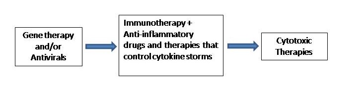
Figure 6: General Therapeutic Plan

This is just a useful therapeutic plan. We will see later that the role of a cytotoxic therapy sometimes can be played by an immunotherapy or an antiviral. Fig. (6) shows a very general plan.

Now we will present several concrete combination therapies. There are certain observations Ref17 that support the existence of synergism between Remdesivir and monoclonal antibodies. Considering the fact that our investigation leads to a combination of antivirals, immunotherapy, and virus – killing medications, the mentioned synergism help us build the treatment shown in Fig. (LABEL:Figure7).

The simplest of our designed therapies is shown in Fig. (7) and Figures (8)-(LABEL:Figure10) show different alternative treatments.

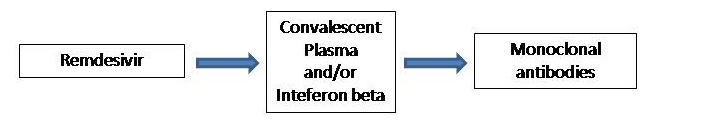
Figure 7: One of the simplest therapies: Remdesivir plus Immunotherapy plus Monoclonal antibodies

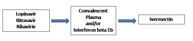
Figure 8: Anti-HIV cocktail plus Immunotherapy plus Ivermectin