Quantifying uncertainty about global and regional economic impacts of climate change
Abstract
The economic impacts of climate change are highly uncertain. Two of the most important uncertainties are the sensitivity of the climate system and the so-called damage functions, which relate climate change to economic damages and benefits. Despite broad awareness of these uncertainties, it is unclear which of them is most important, both on the global as well as the regional level. Here we apply different damage functions to data from climate models with vastly different climate sensitivities, and find that uncertainty in both climate sensitivity and economic damage per degree of warming are of similar importance for the global economic impact. Increasing the climate sensitivity or the sensitivity of the damage function both increases the economic damages globally. Yet, at the country-level the effect varies depending on the initial temperature as well as how much the country warms. Our findings emphasise the importance of including these uncertainties in estimates of future economic impacts, as they both are vital for the resulting impacts and thus policy implications.
1 Introduction
Future projections of the economic impacts of climate change are highly uncertain. On the climate side, the most important uncertainty is how sensitive the climate system is to increasing amounts of greenhouse gases. On the economic side, the most important uncertainty is the relationship between climate change and economic impacts, often expressed in models by so-called damage functions. But which of these uncertainties is most important when assessing the economics impacts of future climate change?
A standard measure of how sensitive the climate is to greenhouse gas emissions is the equilibrium climate sensitivity (ECS) (IPCC, 2013). This is how much the global mean surface air temperature will eventually increase when the amount of atmospheric CO2 is doubled. For decades the estimated range for ECS has been 1.5-4.5C (IPCC, 2013; Charney et al., 1979). However, among the newest generation of climate models, there are several models with ECS above 5C (e.g. Zelinka et al., 2020). Since economic impacts of climate change are currently mostly calculated from temperature (van Vuuren et al., 2012), it is important to understand the implications of this uncertainty.
In economics, integrated assessment models (IAMs) for climate and economy are essential tools for simulating the economic impacts of climate change (see e.g. Nordhaus, 1992; Ackerman et al., 2009; Weyant, 2017). These models link climate and the economy by expressing changes in economic productivity (also called economic damages or benefits) as a function of the climate state, often represented by surface air temperature. So far, most damage functions have been applied to the global mean temperature (Nordhaus, 2018; Weitzman, 2012) or to the temperature of large regions (Nordhaus and Yang, 1996; Hope, 2011; Anthoff and Tol, 2014), and therefore cannot tell us how individual countries or smaller regions will be impacted. The damage function is also an aspect of IAMs that has been criticised for being particularly uncertain (see e.g. Ackerman et al., 2009; Weitzman, 2010; Howard and Sterner, 2017; Diaz and Moore, 2017), yet it is a crucial part of assessing the impacts of climate change.
Hassler et al. (2018) have previously found, using an IAM, that the importance of uncertainty in climate sensitivity and sensitivity in damage functions are of similar magnitude globally. Here, we aim to compare these two uncertainties using a different method, which also allows us to investigating their importance at the regional and country level.
We investigate the global and regional economic impacts of climate change by constructing regional damage functions that aggregate up to the global damages from already existing global damage functions. Our approach builds on the method used by Zheng et al. (2020), by applying a damage function to climate model data, but our focus is on future projections dominated by greenhouse gas emissions, rather than aerosols. Additionally, we span the range of ECS and damage function uncertainties by using a low and a high climate sensitivity model, as well as a relatively insensitive and a relatively sensitive damage function.
2 Method
2.1 Climate model data and scenarios
We used data from a high-sensitivity model, the Community Earth System Model version 2 (CESM2, ECS=5.3C)(Danabasoglu et al., 2020), and a low sensitivity model, the Norwegian Earth System Model (NorESM2, ECS=2.5C)(Seland et al., 2020). Both participate in the 6th phase of the Coupled Model Intercomparison Project (CMIP6) (Eyring et al., 2015), and together the two models span most of the ECS interval of 1.8–5.6 K found in CMIP6 (Zelinka et al., 2020).
Specifically, the climate model data used were the surface air temperatures from the four future emission scenarios used in CMIP6 (Riahi et al., 2017; O'Neill et al., 2016), called shared socioeconomic pathways (SSPs). Since the scenarios go from 2015 to 2100, we also used the last years from runs with historical emission, because our base year here is year 2000. The scenarios are named using two numbers, where the first refers to the narrative (evolution of society and natural systems) (O’Neill et al., 2014), and the second refer to the radiative forcing at the end of the century (Moss et al., 2010). Generally, lower (higher) numbers refer to lower (higher) emissions, and thus a lower (higher) temperature increase. A short summary of the scenarios are given in table 1.
| Scenario | Narrative | 2100 Forcing | Pathway of |
|---|---|---|---|
| name | (W/m2) | forcing | |
| SSP1-2.6 | Sustainability | 2.6 | Peak and decline |
| (Low challenges to | |||
| mitigation and adaptation) | |||
| SSP2-4.5 | Middle of the Road | 4.5 | Stabilising |
| (Medium challenges to | |||
| mitigation and adaptation) | |||
| SSP3-7.0 | Regional Rivalry | 7.0 | Rising |
| (High challenges to | |||
| mitigation and adaptation) | |||
| SSP5-8.5 | Fossil-fueled Development | 8.5 | Rising |
| (High challenges to mitigation, | |||
| low challenges to adaptation) |
2.2 Damage functions and economic impacts
2.2.1 Global damage functions
Integrated assessment models typically incorporate global (or aggregate) economic damages from global warming as a reduction in global total factor productivity (TFP), a measure of the productivity of a set of factors of production (such as physical capital and labour) taken as a whole. These damages can therefore be expressed as a fraction of global GDP, holding fixed productive inputs such as capital and labour, that varies with , the change in the global surface air temperature in year from the pre-industrial temperature.
That fraction, , is typically represented by an increasing convex function with the following functional form (see e.g. Dietz and Stern, 2015):
| (1) |
where is a coefficient chosen to match estimates of aggregate damages from global warming. A change in the global temperature from to would therefore lead to a percentage change in global TFP (and hence global GDP, holding inputs fixed) given by
| (2) |
where , and is the global mean surface air temperature in years 2000, 1850 (pre-industrial), and year , respectively.
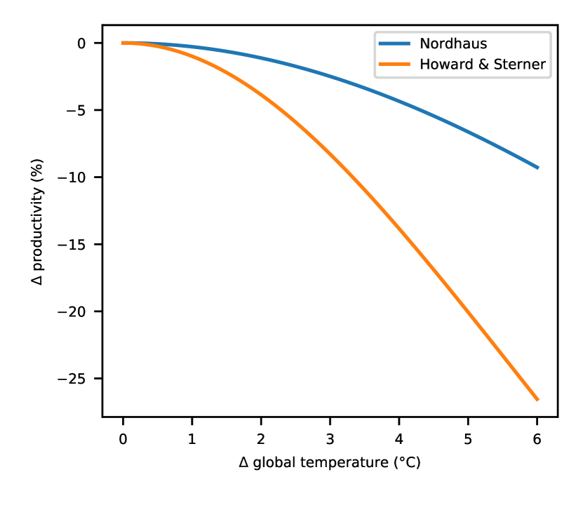
The damage function developed by Nordhaus (Nordhaus, 1992, 2018) is one of the most commonly used damage functions and sets (with unit 1/C2) (see blue line in figure 1). Like many other damage functions, the Nordhaus damage function is only based on estimates of damages up to 3C (Tol, 2011; Stern, 2013), and is strictly speaking not valid for temperature increases beyond that. However, it is often extrapolated to higher temperature changes, and it is also criticised for being too optimistic, in that it may underestimate damages at large temperature increases (Stern, 2013; Revesz et al., 2014). We therefore use this as our low sensitivity damage function.
Another, more sensitive damage function, is the one estimated by Howard and Sterner (2017), which sets (see orange line in figure 1). We use this as our high sensitivity damage function. At 1C warming, the difference in productivity between the two functions is less than 1%, but as we approach 6C warming the difference is more than 17%, ranging from -9.3% with the Nordhaus function to -26.5% with the Howard & Sterner function.
2.2.2 Constructing regional damage functions
In order to study how global warming affects regional economies, we constructed functions that capture how regional productivity varies with regional, rather than the global, surface air temperature. These functions are chosen so that the sum of regional variations across the globe matches estimates of global damages stemming from global warming. The full details on the calculations of the regional damage function is given in the appendix.
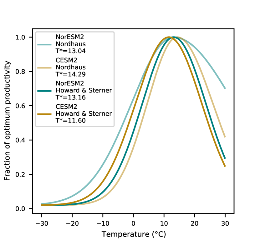
To operationalize the regional productivity function , we used an inverse -shaped function that depends on four parameters:
| (3) |
where is the temperature in region at time , is the optimal temperature (given in C) at which attains its maximum of 1, and and determine the steepness of the decline on either side of the optimal temperature. The lower bound is set to 0.02. The remaining three parameters of the function H are chosen so that the aggregate damages from global warming implied by it match those delivered by the aggregate damage function D in equation 2 at three different global temperature changes ranging from 1 to 5C, noting that the temperature in any particular region depends on the global temperature via a statistical downscaling model derived from runs of CESM2 and NorESM2 (see the appendix for details). We used the downhill simplex equation to solve these three nonlinear equations in the three unknowns , , and . The resulting functions are shown in figure 2 (and the parameters can be found in supplementary table 1). Note that the three parameters are unique for each climate model–damage function combination. And the resulting regional damages compared to the global damages are shown in supplementary figures 7 and 8. As seen in the figures, the regional damage functions are not prefect fits for the global damage functions. But considering the large uncertainties for these functions, the resulting regional damage functions seem reasonable enough for our purpose.
2.3 Application of the damage function on the climate data
After constructing the regional damage functions, we applied them to the climate model data. First, we calculated the annual spatial temperatures and re-gridded it to fit our 11 population and GDP data grid. Then we calculated the fraction of optimum productivity for each year with the regional damage function.
The 2000 temperature was calculated from a historical run, using the years 1996-2004. We used this to calculate the relative change in optimum productivity from 2000. Which was finally used to calculate the relative change in productivity.
3 Results
3.1 Global economic impacts
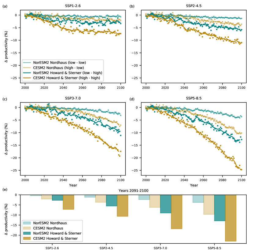
Our results show that global warming decreases the global economic productivity, but the size of these economic damages is highly dependent on the sensitivity of both the climate and the damage function (see fig. 3). Both changing to a more sensitive climate model and a more sensitive damage function increases the damages. Also, the differences between models and damage functions grow as we reach higher temperatures, as seen from both the increasing distance between the lines with time in each SSP scenario, and the larger distance between lines in the higher emissions scenarios. While the range in productivity due to the two damage functions shown here is slightly larger than that of the two climate models, the results indicate that the span of damages due to uncertainty in climate sensitivity and uncertainty associated with damage functions are of a similar magnitude globally, supporting previous work (Hassler et al., 2018).
3.2 Regional economic impacts
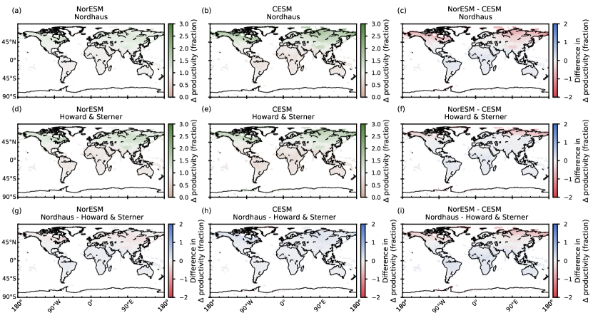
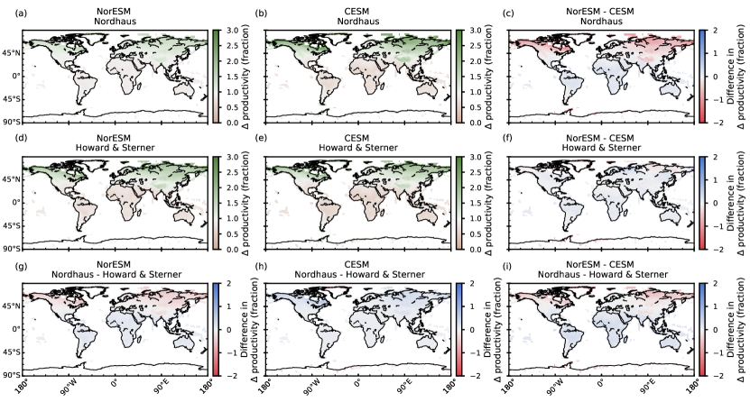
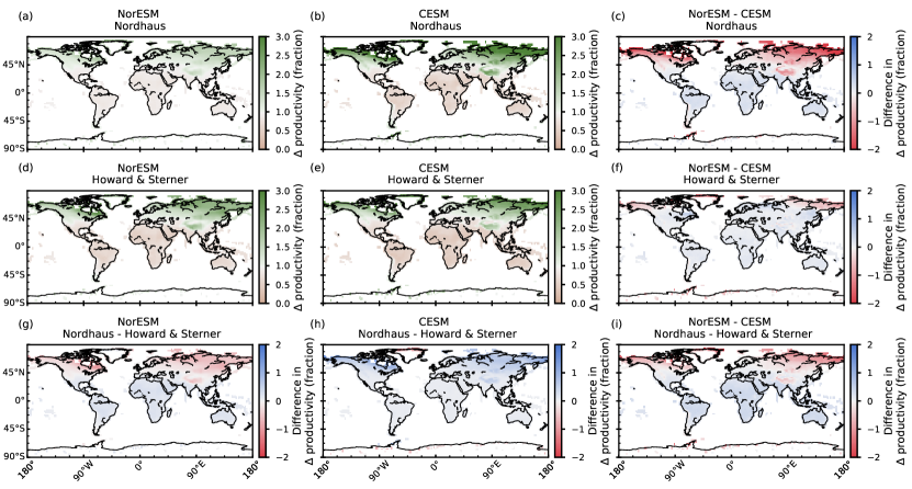
However, the global estimates of economic impacts of climate change hide a lot of heterogeneity at the regional level. Regionally, our calculations predict decreasing productivity for most of the globe, except in the northern high latitudes and the Tibetan Plateau (fig. 4). Figure 4 a,b,d,e shows how the fraction of the optimum productivity has changed from year 2000 to the end of the century in the SSP5-8.5 scenario for the four climate model–damage function combinations. The other scenarios have the same main patterns but of smaller magnitude (see supplementary figures 1-3). While the area with increased productivity (green) might seem vast, much of the area has a small population and economy, and thus does not contribute much to the global productivity.
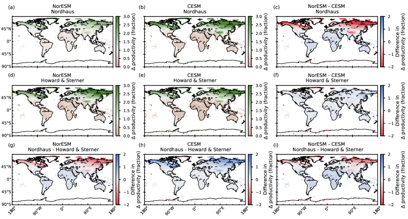
Also, changing between climate models and/or damage functions has different effects in different areas. If we start with the low–low combination (low climate sensitivity - low sensitivity damage function), going to a high sensitivity in either climate model (high–low, fig. 4 c) or damage function (low–high, fig. 4 g) increases the productivity in cold areas, and decreases the productivity in warm areas. But if we start with either the high sensitivity climate model (high–low) or damage function (low–high), and move to the high–high combination (fig. 4 f and h, respectively) the productivity decreases almost everywhere.
This can be understood from the different temperature increases between models, and the different optimum temperatures and slopes of the regional damage functions (see figure 2 and supplementary table 1 for details). When going from the low–low to the low–high combination we have the same warming and approximately the same optimum temperature. The larger increase in productivity in the cold regions and decrease in the warm regions is thus due to the steeper slopes of the damage function, making the regions move faster toward or away from the optimum temperature. If we instead move from the low–low to the high–low combination we still have a similar optimum temperature and steeper slopes. Additionally, this effect is strengthened by the higher temperature increase. In the other case, starting from the low–high or the high–low combination and going to the high–high combination, we have a different situation. Now the slopes are not changing much, but the optimum temperature is lower for the high–high combination. This means that fewer regions have the potential to increase their productivity, and more regions will cross over the optimum temperature and start decreasing their productivity. Additionally, the baseline temperature difference between the models plays a part when changing model.
3.3 Large variation between countries
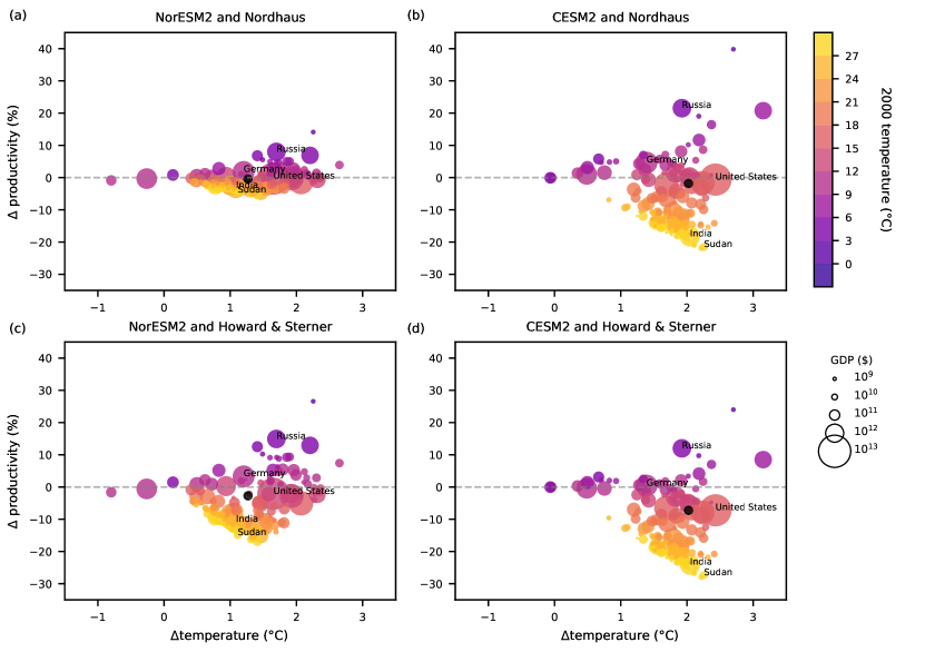
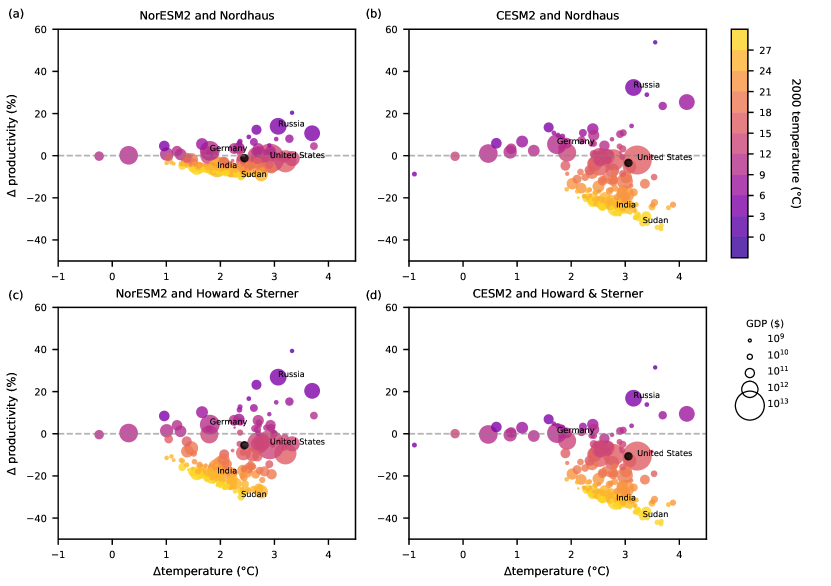
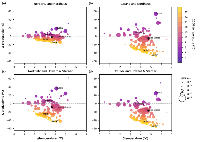
On the country level, as indicated by figure 4, it is the countries with a cool climate that benefit, while the warm countries suffer damages. Figure 5 shows how the temperature and productivity change from 2000 to the end of the century for each country in each climate model–damage function combination for SSP5-8.5 (for the other SSPs see supplementary figures 4-6). Like the global average, the country-level average takes into account each country’s economic activity, measured in gross domestic product (GDP) (indicated by size of circle), and population in year 2000. The colour of the circles show the population-weighted temperature in year 2000. Again, the same three factors that explain figure 4 are important for each country’s change in productivity, as well as the countries’ distribution of population and economic activity. We see that most countries will experience economic impacts that are very different from the global average (black dot).
Some examples of how countries may be impacted in each scenario and climate model–damage function combination are shown in fig. 6. The United States, the biggest country-level economy, nicely follows what we saw for the global productivity (fig. 3 e), while other countries show very different responses. Russia is one of the countries that benefit from climate change independent of scenario and combination, while India and Sudan clearly see economic damages under all circumstances. However, these countries do not follow the same increase in effect with increasing sensitivity as seen globally and for the United States. On the regional level it is not clear that increasing the climate sensitivity and/or sensitivity of the damage function increases the economic impacts.
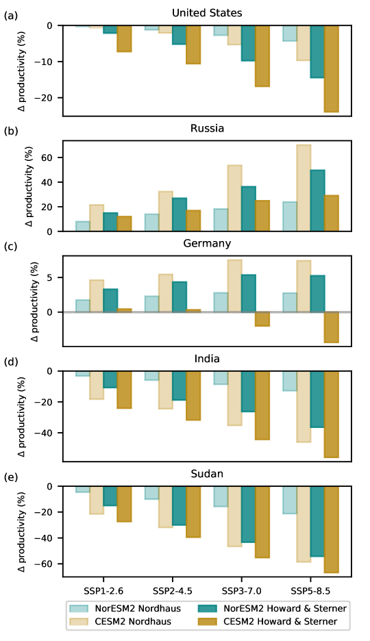
Another interesting group of countries is the one with relatively small impacts that lie close to the zero line in figure 5. Germany (fig. 6 c) is a nice example of these, and we see that whether the country will see benefits or damages due to climate change depends on both the scenario and the climate model–damage function combination. This is because Germany has a temperature lower than, yet close to, the optimal temperature (10.0C in NorESM2, 10.4C in CESM2) in year 2000. As the climate warms, as decided by both the scenario and the climate model, Germany might cross the optimum temperature. When crossing the optimum temperature, the productivity starts to decrease, and if moving too far away from the optimum temperature the end productivity could be lower than at the start point in year 2000, depending on the slopes of the damage function.
4 Discussion
Our results show how the large uncertainties in climate sensitivity and damage functions result in large uncertainties in economic impacts. This points out how important it is to include uncertainty estimates when calculating economic impacts of climate change. Particularly, this is important when using estimates of economic impacts for policy purposes, like for example the US government does (Auffhammer, 2018). The study also points out how different the economic impacts of climate change can be between regions. Especially, we see how the regional uncertainty in economic impacts can be very different from the global.
In a full economic model, the economic impacts will feed back on the emissions. With economic damages, consumption will decrease, and consequently the emissions (and thus the warming) will be lower (and visa versa for economic benefits). In our work, future emissions are already set by the SSP scenarios, and this climate-economy feedback is therefore not included. However, the study still gives important insights into the relative importance of the climate sensitivity and sensitivity of the damage function. Both of these are important for the size of the climate-economy feedback, and this could be a step towards assessing the feedback’s uncertainty.
Our calculations are based on the assumption that the population growth is constant in time and space, and the actual future population growth and migration could therefore result in a different future global productivity. If, for example, people living in less productive areas move northward into more productive areas, the global productivity would decrease less with warming. Such migration to more productive areas are indeed expected, and even simulated in some models (Conte et al., 2020).
An important remaining question is how good of a proxy temperature is for climate change. In the damage functions employed here, it is assumed that the global temperature represents global climate change well. This is probably a reasonable assumption, but it might not hold as well when we construct regional damage functions that look at regional temperature. Changes in other climate variables, like rainfall, sea level rise or extreme events, do not necessarily have the same distribution patterns as temperature change (IPCC, 2013). Sea-level rise, for example, should only affect regions with a coast line, but when temperature is the only input to the damage function, the inherent damages from sea-level rise in the global damage function will be distributed depending on temperature in the regional function. Thus the impacts of climate change that do not follow the temperature distribution could be wrongly distributed.
In our study, we have used damage functions that calculate the impact of climate change on the economic output rather than on the economic growth rate. Yet, this is an area of some debate (see e.g. Moore and Diaz, 2015; Burke et al., 2015). Since even a small change in the growth rate could lead to large economic impacts in the long run, such damage functions could be even more sensitive than the high sensitivity damage function employed here.
5 Conclusion
We have found that the uncertainties in climate sensitivity and damage functions are of similar magnitude globally, but differ a lot regionally. What is clear from this study is that progress toward reliable assessments of economic damages due to climate change will require both more constrained estimates of the climate sensitivity and improved damage functions. Especially, this is important when economic models are used for policy purposes (see e.g. Burke et al., 2016; Hassler et al., 2018). We see that the global productivity tells us little about what will happen regionally or in a given country. The regional productivity could also be more impacted by changes that are not as well represented by the annual mean surface air temperature, such as rainfall or extreme events. A focus on constructing regional damage functions will therefore be important.
Acknowledgements
This work was supported by the Norwegian Research Council through grant 281071. We acknowledge the World Climate Research Programme, which, through its Working Group on Coupled Modelling, coordinated and promoted CMIP6. We thank the climate modelling groups for producing and making available their model output, the Earth System Grid Federation (ESGF) for archiving the data and providing access, and the multiple funding agencies who support CMIP6 and ESGF.
Competing Interests statement
The authors declare no competing interests.
Data availability
All NorESM2 and CESM2 simulation output is available through the Earth System Grid Federation’s (ESGF) CMIP6 search interface (https://esgf-node.llnl.gov/search/cmip6/) under ‘source ID’ NorESM2-LM and CESM2, respectively, and ‘experiment ID’ historical, ssp126, ssp245, ssp370 and ssp585.
Population and GDP data from the Geographically based Economic data (G-Econ) site, version 2.11 (Nordhaus et al., 2006), is no longer available on the web site, but is available from the authors on request.
References
- (1)
- Ackerman et al. (2009) Ackerman, F., DeCanio, S. J., Howarth, R. B. and Sheeran, K. (2009), ‘Limitations of integrated assessment models of climate change’, Climatic change 95(3-4), 297–315. doi:https://doi.org/10.1007/s10584-009-9570-x.
-
Anthoff and Tol (2014)
Anthoff, D. and Tol, R. S. J. (2014), ‘The climate Framework for Uncertainty, Negotiation and Distribution
(FUND), technical description, version 3.9’.
http://www.fund-model.org/files/documentation/Fund-3-9-Scientific-Documentation.pdf - Auffhammer (2018) Auffhammer, M. (2018), ‘Quantifying economic damages from climate change’, Journal of Economic Perspectives 32(4), 33–52. doi:.1257/jep.32.4.33.
- Burke et al. (2016) Burke, M., Craxton, M., Kolstad, C. D., Onda, C., Allcott, H., Baker, E., Barrage, L., Carson, R., Gillingham, K., Graff-Zivin, J., Greenstone, M., Hallegatte, S., Hanemann, W. M., Heal, G., Hsiang, S., Jones, B., Kelly, D. L., Kopp, R., Kotchen, M., Mendelsohn, R., Meng, K., Metcalf, G., Moreno-Cruz, J., Pindyck, R., Rose, S., Rudik, I., Stock, J. and Tol, R. S. J. (2016), ‘Opportunities for advances in climate change economics’, Science 352(6283), 292–293. doi:10.1126/science.aad9634.
- Burke et al. (2015) Burke, M., Hsiang, S. M. and Miguel, E. (2015), ‘Global non-linear effect of temperature on economic production’, Nature 527(7577), 235. doi:10.1038/nature15725.
- Charney et al. (1979) Charney, J. G., Arakawa, A., Baker, D. J., Bolin, B., Dickinson, R. E., Goody, R. M., Leith, C. E., Stommel, H. M. and Wunsch, C. I. (1979), Carbon dioxide and climate: a scientific assessment, National Academy of Sciences, Washington, DC.
- Conte et al. (2020) Conte, B., Desmet, K., Nagy, D. K. and Rossi-Hansberg, E. (2020), ‘Local sectoral specialization in a warming world’, NBER working paper (w28163). doi:10.3386/w28163.
- Danabasoglu et al. (2020) Danabasoglu, G., Lamarque, J.-F., Bacmeister, J., Bailey, D. A., DuVivier, A. K., Edwards, J., Emmons, L. K., Fasullo, J., Garcia, R., Gettelman, A., Hannay, C., Holland, M. M., Large, W. G., Lauritzen, P. H., Lawrence, D. M., Lenaerts, J. T. M., Lindsay, K., Lipscomb, W. H., Mills, M. J., Neale, R., Oleson, K. W., Otto-Bliesner, B., Phillips, A. S., Sacks, W., Tilmes, S., Kampenhout, L., Vertenstein, M., Bertini, A., Dennis, J., Deser, C., Fischer, C., Fox-Kemper, B., Kay, J. E., Kinnison, D., Kushner, P. J., Larson, V. E., Long, M. C., Mickelson, S., Moore, J. K., Nienhouse, E., Polvani, L., Rasch, P. J. and Strand, W. G. (2020), ‘The Community Earth System Model Version 2 (CESM2)’, Journal of Advances in Modeling Earth Systems 12(2). doi:10.1029/2019ms001916.
- Diaz and Moore (2017) Diaz, D. and Moore, F. (2017), ‘Quantifying the economic risks of climate change’, Nature Climate Change 7(11), 774–782. doi:10.1038/nclimate3411.
- Dietz and Stern (2015) Dietz, S. and Stern, N. (2015), ‘Endogenous growth, convexity of damage and climate risk: how Nordhaus’ framework supports deep cuts in carbon emissions’, The Economic Journal 125(583), 574–620. doi:10.1111/ecoj.12188.
- Eyring et al. (2015) Eyring, V., Bony, S., Meehl, G. A., Senior, C., Stevens, B., Stouffer, R. J. and Taylor, K. E. (2015), ‘Overview of the Coupled Model Intercomparison Project Phase 6 (CMIP6) experimental design and organisation’, Geoscientific Model Development Discussions 8(12), 10539–10583. doi:10.5194/gmdd-8-10539-2015.
- Hassler et al. (2018) Hassler, J., Krusell, P. and Olovsson, C. (2018), ‘The Consequences of Uncertainty: Climate Sensitivity and Economic Sensitivity to the Climate’, Annual Review of Economics 10(1), 189–205. doi:10.1146/annurev-economics-080217-053229.
- Hope (2011) Hope, C. (2011), ‘The social cost of CO2 from the PAGE09 model’, Economics discussion paper (2011-39). doi:10.2139/ssrn.1973863.
- Howard and Sterner (2017) Howard, P. H. and Sterner, T. (2017), ‘Few and Not So Far Between: A Meta-analysis of Climate Damage Estimates’, Environmental and Resource Economics 68(1), 197–225. doi:10.1007/s10640-017-0166-z.
-
IPCC (2013)
IPCC (2013), Climate Change 2013:
The Physical Science Basis. Contribution of Working Group I
to the Fifth Assessment Report of the Intergovernmental Panel on
Climate Change, Cambridge University Press, Cambridge, United Kingdom
and New York, NY, USA.
https://www.ipcc.ch/report/ar5/wg1/ -
Krusell and Smith, Jr. (2020)
Krusell, P. and Smith, Jr., A. A. (2020), ‘Climate Change Around the World’, Slide
presentation.
http://www.econ.yale.edu/smith/bu2.pdf - Moore and Diaz (2015) Moore, F. C. and Diaz, D. B. (2015), ‘Temperature impacts on economic growth warrant stringent mitigation policy’, Nature Climate Change 5(2), 127–131. doi:10.1038/nclimate2481.
- Moss et al. (2010) Moss, R. H., Edmonds, J. A., Hibbard, K. A., Manning, M. R., Rose, S. K., Van Vuuren, D. P., Carter, T. R., Emori, S., Kainuma, M., Kram, T. and others (2010), ‘The next generation of scenarios for climate change research and assessment’, Nature 463(7282), 747. doi:10.1038/nature08823.
- Nordhaus (2018) Nordhaus, W. (2018), ‘Evolution of modeling of the economics of global warming: changes in the DICE model, 1992–2017’, Climatic Change 148(4), 623–640. doi:https://doi.org/10.1007/s10584-018-2218-y.
- Nordhaus et al. (2006) Nordhaus, W., Azam, Q., Corderi, D., Hood, K., Victor, N. M., Mohammed, M., Miltner, A. and Weiss, J. (2006), ‘The G-Econ database on gridded output: methods and data’, Yale University, New Haven 6.
- Nordhaus (1992) Nordhaus, W. D. (1992), ‘An optimal transition path for controlling greenhouse gases’, Science 258(5086), 1315–1319. doi:10.1126/science.258.5086.1315.
- Nordhaus and Yang (1996) Nordhaus, W. D. and Yang, Z. (1996), ‘A regional dynamic general-equilibrium model of alternative climate-change strategies’, The American Economic Review pp. 741–765.
- O'Neill et al. (2016) O'Neill, B. C., Tebaldi, C., van Vuuren, D. P., Eyring, V., Friedlingstein, P., Hurtt, G., Knutti, R., Kriegler, E., Lamarque, J.-F., Lowe, J., Meehl, G. A., Moss, R., Riahi, K. and Sanderson, B. M. (2016), ‘The Scenario Model Intercomparison Project (ScenarioMIP) for CMIP6’, Geoscientific Model Development 9(9), 3461–3482. doi:10.5194/gmd-9-3461-2016.
- O’Neill et al. (2014) O’Neill, B. C., Kriegler, E., Riahi, K., Ebi, K. L., Hallegatte, S., Carter, T. R., Mathur, R. and van Vuuren, D. P. (2014), ‘A new scenario framework for climate change research: the concept of shared socioeconomic pathways’, Climatic change 122(3), 387–400. doi:10.1007/s10584-013-0905-2.
- Revesz et al. (2014) Revesz, R. L., Arrow, K. J., Goulder, L. H., Howard, P., Kopp, R. E., Livermore, M. A., Oppenheimer, M. and Sterner, T. (2014), ‘Improve economic models of climate change’, Nature 508, 173–175. doi:10.1038/508173a.
- Riahi et al. (2017) Riahi, K., Van Vuuren, D. P., Kriegler, E., Edmonds, J., O’neill, B. C., Fujimori, S., Bauer, N., Calvin, K., Dellink, R., Fricko, O. et al. (2017), ‘The shared socioeconomic pathways and their energy, land use, and greenhouse gas emissions implications: an overview’, Global Environmental Change 42, 153–168. doi:10.1016/j.gloenvcha.2016.05.009.
- Seland et al. (2020) Seland, Ø., Bentsen, M., Graff, L. S., Olivié, D., Toniazzo, T., Gjermundsen, A., Debernard, J. B., Gupta, A. K., He, Y., Kirkevåg, A., Schwinger, J., Tjiputra, J., Aas, K. S., Bethke, I., Fan, Y., Griesfeller, J., Grini, A., Guo, C., Ilicak, M., Karset, I. H. H., Landgren, O., Liakka, J., Moseid, K. O., Nummelin, A., Spensberger, C., Tang, H., Zhang, Z., Heinze, C., Iverson, T. and Schulz, M. (2020), ‘The Norwegian Earth System Model, NorESM2 – Evaluation of theCMIP6 DECK and historical simulations’, Geoscientific Model Development . doi:10.5194/gmd-2019-378.
- Stern (2013) Stern, N. (2013), ‘The Structure of Economic Modeling of the Potential Impacts of Climate Change: Grafting Gross Underestimation of Risk onto Already Narrow Science Models’, Journal of Economic Literature 51(3), 838–859. doi:10.1257/jel.51.3.838.
- Tol (2011) Tol, R. S. J. (2011), ‘The Social Cost of Carbon’, Annual Review of Resource Economics 3(1), 419–443. doi:10.1146/annurev-resource-083110-120028.
- van Vuuren et al. (2012) van Vuuren, D. P., Bayer, L. B., Chuwah, C., Ganzeveld, L., Hazeleger, W., van den Hurk, B., Van Noije, T., O’Neill, B. and Strengers, B. J. (2012), ‘A comprehensive view on climate change: coupling of earth system and integrated assessment models’, Environmental Research Letters 7(2), 024012. doi:10.1088/1748-9326/7/2/024012.
- Weitzman (2010) Weitzman, M. L. (2010), ‘What is the ”damage function” for global warming — and what difference might it make?’, Climate Change Economics 01(01), 57–69. doi:10.1142/s2010007810000042.
- Weitzman (2012) Weitzman, M. L. (2012), ‘GHG Targets as Insurance Against Catastrophic Climate Damages’, Journal of Public Economic Theory 14(2), 221–244. doi:10.1111/j.1467-9779.2011.01539.x.
- Weyant (2017) Weyant, J. (2017), ‘Some Contributions of Integrated Assessment Models of Global Climate Change’, Review of Environmental Economics and Policy 11(1), 115–137. doi:10.1093/reep/rew018.
- Zelinka et al. (2020) Zelinka, M. D., Myers, T. A., McCoy, D. T., Po-Chedley, S., Caldwell, P. M., Ceppi, P., Klein, S. A. and Taylor, K. E. (2020), ‘Causes of higher climate sensitivity in CMIP6 models’, Geophysical Research Letters . doi:10.1029/2019GL085782.
- Zheng et al. (2020) Zheng, Y., Davis, S. J., Persad, G. G. and Caldeira, K. (2020), ‘Climate effects of aerosols reduce economic inequality’, Nature Climate Change 10(3), 220–224. doi:10.1038/s41558-020-0699-y.
Supplementary Material
Appendix
To look at regional differences in productivity stemming from global warming, we needed a regional function mapping regional surface air temperatures into regional productivity. Following Krusell and Smith, Jr. (2020), we constructed such a function so that regional variations in productivity, when summed across all regions, match the global changes in productivity delivered by the aggregate damage function (equation 2).
To do this, we used a simple economic model of regional GDP:
| (4) |
where, in region (or grid-cell) in year , is GDP, is the physical capital stock, and is the effective supply of labour, measured in so-called “efficiency units” which capture how productive workers are. The coefficients and are the shares of income (GDP) going to capital and labour, respectively. We assume further that the effective supply of labour evolves according to:
| (5) |
where, in region in year , is the population and is the number of efficiency units per person. Population is assumed to grow at rate . The first component of the number of efficiency units, , does not depend on regional temperature and is assumed to grow at rate . The second component of the number of efficiency units, , does depend on regional temperature: it captures on how changes in regional temperature, , affect the regional productivity of labour. The function governing this component of regional productivity has an inverse -shape and is bounded between 0 and 1.
Finally, we assume that at any point in time capital is freely mobile across regions so that the marginal product of capital (i.e., the extra amount of GDP generated by an incremental amount of additional capital) is equated across regions. Consequently, regional capital-to-labour ratios, , are also equalised, implying in turn that global GDP in year , , where is the number of regions, has a simple expression:
| (6) |
where is the global capital stock.111Krusell and Smith, Jr. (2020) show that even when capital markets are closed completely optimal accumulation of capital in each region leads the marginal product of capital to be approximately equalised across regions. Thus the assumption of free capital mobility underlying the formulas in this paper appears to be an innocuous one. Substituting equation (5) into equation (6) yields an expression for global GDP in year depends explicitly on the set of regional temperatures:
| (7) |
To derive an analogous expression for global GDP that depends only on the global temperature, we used a statistical downscaling model that relates regional temperature to global temperature:
| (8) |
To obtain the region-specific responsiveness coefficients , we proceeded in three steps. First, we calculated the global temperature change from pre-industrial to year 2000, which is our reference year. Second, we calculated the temperatures in year 2000 for each grid cell (). Here we used surface air temperature from three historical runs by the climate model, and calculated the average of these three runs using the nine years around 2000 (1996-2004). Finally, we calculated how each grid cell’s temperature changes relative to the global temperature, the responsiveness coefficients (). These we calculated by using five different model runs: historical, SSP1-2.6, SSP2-4.5, SSP3-7.0 and SSP5-8.5. For each run, the difference between the first and the last five years was calculated, and each grid cell’s change was divided by the global temperature change. The average of these five coefficients was then used as the final set of responsiveness coefficients for each of the two models (e.i. NorESM2 and CESM2).
Armed with the statistical downscaling model in equation (8), equation (7) can now be rewritten:
| (9) |
where , , and is efficiency units per person in region in 2000. Given a regional productivity function (in our case equation 3), a change in the global temperature from to would lead to a percentage change in global GDP (again holding inputs fixed) equal to:
| (10) |
The goal now is to choose (equation 3) so that the two “damage functions”, and , the first taken from existing estimates of global damages from climate change and the second derived from the simple economic model of regional damages from climate change outlined here, agree for different values of the global temperature .
Regional population and GDP data for the year 2000 are taken from the G-Econ database, version 2.11 (Nordhaus et al., 2006). The are chosen by solving the following two equations for and in each region:
The first of these equations ensures that regional GDP in year 2000 equals its value in the data and the second of these equations imposes that the marginal product of capital in each region is equated to a common rate of return (net of depreciation), here set to 2.53%. Capital’s share of income, , is set to 0.36.
| Damage function | Model | T∗ | ||
|---|---|---|---|---|
| Nordhaus | NorESM2 | 13.0 | 0.00267 | 0.00127 |
| Nordhaus | CESM2 | 14.3 | 0.00522 | 0.00367 |
| Howard & Sterner | NorESM2 | 13.2 | 0.00476 | 0.00453 |
| Howard & Sterner | CESM2 | 11.6 | 0.00420 | 0.00434 |
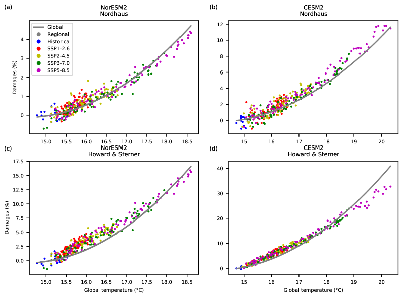
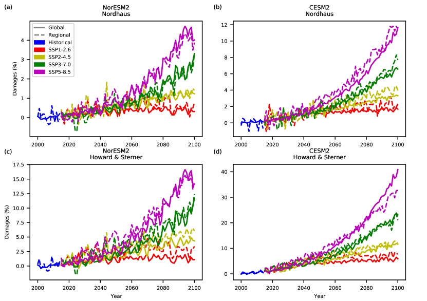
Each year from historical run and the SSP scenarios are plotted for both the global (line) and the regional (dashed), for the four climate model damage function combinations.