11institutetext: Ryan G. McClarren22institutetext: University of Notre Dame
Department of Aerospace and Mechanical Engineering
Notre Dame, IN 46556, USA
22email: rmcclarr@nd.edu
33institutetext: James A. Rossmanith44institutetext: Iowa State University
Department of Mathematics
Ames, IA 50011-2104, USA
44email: rossmani@iastate.edu
55institutetext: Minwoo Shin66institutetext: University of Notre Dame
Department of Aerospace and Mechanical Engineering
Notre Dame, IN 46556, USA
66email: mshin@nd.edu

Semi-implicit Hybrid Discrete (HNT)subscriptsuperscriptH𝑇𝑁\left(\text{H}^{T}_{N}\right) Approximation of Thermal Radiative Transfer

Ryan G. McClarren    James A. Rossmanith    Minwoo Shin111Corresponding Author
(Received: date / Accepted: date)
Abstract

The thermal radiative transfer (TRT) equations form an integro-differential system that describes the propagation and collisional interactions of photons. Computing accurate and efficient numerical solutions TRT are challenging for several reasons, the first of which is that TRT is defined on a high-dimensional phase space that includes the independent variables of time, space, and velocity. In order to reduce the dimensionality of the phase space, classical approaches such as the PN (spherical harmonics) or the SN (discrete ordinates) ansatz are often used in the literature. In this work, we introduce a novel approach: the hybrid discrete (HNTsubscriptsuperscriptabsent𝑇𝑁{}^{T}_{N}) approximation to the radiative thermal transfer equations. This approach acquires desirable properties of both PN and SN, and indeed reduces to each of these approximations in various limits: HN1subscriptsuperscriptabsent1𝑁{}^{1}_{N} \equiv PN and H0Tsubscriptsuperscriptabsent𝑇0{}^{T}_{0} \equiv ST. We prove that HNTsubscriptsuperscriptabsent𝑇𝑁{}^{T}_{N} results in a system of hyperbolic partial differential equations for all T1𝑇1T\geq 1 and N0𝑁0N\geq 0. Another challenge in solving the TRT system is the inherent stiffness due to the large timescale separation between propagation and collisions, especially in the diffusive (i.e., highly collisional) regime. This stiffness challenge can be partially overcome via implicit time integration, although fully implicit methods may become computationally expensive due to the strong nonlinearity and system size. On the other hand, explicit time-stepping schemes that are not also asymptotic-preserving in the highly collisional limit require resolving the mean-free path between collisions, making such schemes prohibitively expensive. In this work we develop a numerical method that is based on a nodal discontinuous Galerkin discretization in space, coupled with a semi-implicit discretization in time. In particular, we make use of a second order explicit Runge-Kutta scheme for the streaming term and an implicit Euler scheme for the material coupling term. Furthermore, in order to solve the material energy equation implicitly after each predictor and corrector step, we linearize the temperature term using a Taylor expansion; this avoids the need for an iterative procedure, and therefore improves efficiency. In order to reduce unphysical oscillation, we apply a slope limiter after each time step. Finally, we conduct several numerical experiments to verify the accuracy, efficiency, and robustness of the HNTsubscriptsuperscriptabsent𝑇𝑁{}^{T}_{N} ansatz and the numerical discretizations.

Keywords:
thermal radiative transfer discontinuous Galerkin discrete hybrid approximation semi-implicit time integration asymptotic-preserving
MSC:
85A25 65M60
journal:

1 Introduction

The thermal radiative transfer (TRT) equations describe the interaction of matter and thermal radiation, and are used in a wide range of applications including remote sensing, glass manufacturing, and combustion siegel . The TRT equations model the propagation, absorption, and emission of photons, as well as the coupling of these dynamics to background media via a material-energy equation. Accurate and efficient numerical solutions of the TRT equations are challenging for several reasons:

  1. 1.

    The TRT equations form an integro-differential system that is posed on a high-dimensional phase space: the time dimension, up to three spatial dimensions, two velocity direction dimensions, and a frequency dimension;

  2. 2.

    Optically thick media introduces stiffness due to the large timescale separation between propagation and collisions;

  3. 3.

    The material-energy coupling equation introduces strong non-linearity.

1.1 Discretization of the phase space

Two broad classes of solution approaches have been used to tackle the TRT equation (1) stochastic methods and (2) deterministic methods; each approach offers their own advantages and disadvantages. The main workhorse of the stochastic approach is the Monte Carlo (MC) method, which is considered one of the most reliable methods in the radiation community fleck ; mcclarren2009modified ; wollaber2016four . Monte Carlo methods produce statistical noise due to under-sampling of the phase space; and therefore, to compensate for this under-sampling, many MC histories are required, which in turns makes the MC calculation expensive. As a result, high performance computing approaches are needed. In the realm of deterministic approaches for the angular dependence, the most popular methods are the discrete ordinates (SN) method carlson ; koch ; lathrop3 ; lathrop2 ; lathrop1 ; pomraning1 and the spherical harmonics (PN) method with various closures lewis ; mcclarren1 ; olson1 ; olson ; pomraning . The advantages of these approaches are that, relative to Monte Carlo, they are less computationally expensive. On the other hand they each suffer from their own specific disadvantages.

The SN approximation scheme creates a system of equations along a discrete set of angular directions that are taken from a specific quadrature set carlson1 ; jarrell ; lau ; thurgood , and angular integrals are calculated via the given quadrature set. The SN method has been the subject of intense research, and many large-scale efficient solution techniques have been developed, including approaches that have been shown to scale on leadership-class computers adams2020provably . The SN method’s main drawback is the phenomenon known as ray effects lathrop3 ; lathrop2 , which arises due to the fact that particles move only along certain directions in the quadrature set. These effects are conspicuously observed in optically thin materials with localized sources or sharp material discontinuities.

On the other hand, the PN method approximates the solution with a spherical harmonics expansion that by construction is rotationally invariant and converges in the L2superscript𝐿2L^{2} sense hauck . The main disadvantage of the PN approach is that it is plagued by Gibbs phenomena (i.e., unphysical oscillations) due to the fact that it is a truncated spectral method and can thereby produce the negative particle concentrations hauck ; mcclarren2008solutions , which is physically undesirable. Additionally, in the PN method, when N𝑁N is small, the wave speeds are reduced because the system eigenvalues can be far from unity. Closures have been developed to deal some of the shortcomings of the PN method, such as the MN method dubroca1999etude ; hauck2011high and other techniques laiu ; zheng2016moment ; hauck2010positive .

1.2 Stiffness

Another challenging aspect in accurately and efficiently solving the thermal radiative transfer (TRT) equations is that the system is inherently stiff. This stiffness is especially pervasive in the diffusive regime (i.e., highly collisional), where there is a large timescale separation between propagation and collisions. The reduction of the kinetic TRT system to a lower dimensional system of partial differential equations (PDEs) via an ansatz such as discrete ordinate (SN) or spherical harmonics (PN) does not alleviate this problem.

From the perspective of numerical methods, the stiffness challenge can be partially overcome via implicit time integration, although fully implicit methods may become computationally expensive due to the strong nonlinearity and system size. On the other hand, explicit time-stepping schemes that are not also asymptotic-preserving in the highly collisional limit require resolving the mean-free path between collisions, making such schemes prohibitively expensive.

An efficient alternative to both fully implicit and fully explicit schemes are semi-implicit schemes, where, at least roughly-speaking, the transport is handled explicitly, while the material coupling term (i.e., collisions) are handled implicitly. For example, Klar et al. klar ; klar1 developed and analyzed an operator splitting approach that was shown to be asymptotically-preserving while at the same time relatively efficient in all regimes. A different semi-implicit approach for TRT was subsequently developed by McClarren et al. mcclarren1 , in which a two-stage second-order Runge-Kutta (RK) scheme was used for the streaming term and the backward Euler scheme was used for the material coupling term. This scheme was also shown to be asymptotic-preserving in the diffusive limit.

1.3 Strong nonlinearity in the material coupling term

In the absence of material coupling, the thermal radiative transfer equations and its various reductions (e.g., PN or SN) represent a system of linear constant-coefficient partial differential equations. The presence of the material coupling term introduces strong nonlinearity. For explicit time-stepping methods this nonlinearity does not pose a direct challenge, although, as mentioned above, explicit methods will then suffer from small time-steps. For fully implicit time-stepping methods the nonlinearity results in large nonlinear algebraic equations that must be inverted in time-step, resulting in significant computational expense. For semi-implicit time-stepping approaches, a nonlinear material coupling term only introduces a local nonlinear algebraic equation (i.e., local on each element), although even this can add computational expense. Fortunately, McClarren, Evans, and Lowrie mcclarren1 showed that the local nonlinear problems presented by a semi-implicit approach can be linearized via a simple Taylor series argument. It was shown that this linearization reduces the computational complexity and does not adversely affect overall accuracy of the method.

1.4 Scope of this work

In order to address some of the shortcomings of classical deterministic methods, we introduce in this work the hybrid discrete (HNTsubscriptsuperscriptabsent𝑇𝑁{}^{T}_{N}) approximation, which hybridizes aspects of the PN and SN methods. The HNTsubscriptsuperscriptabsent𝑇𝑁{}^{T}_{N} approximation is equivalent to spherical harmonics (PN) approximation when the number of the discretized velocity space (T𝑇T) is one and only depends on the order of spherical harmonics basis functions (N𝑁N). Also, it is equivalent to the discrete ordinate (SN) method for a certain quadrature set. By hybridizing PN and SN, the HNTsubscriptsuperscriptabsent𝑇𝑁{}^{T}_{N} approximation is able to acquire beneficial properties of both of these classical approaches. We prove that HNTsubscriptsuperscriptabsent𝑇𝑁{}^{T}_{N} results in a system of hyperbolic partial differential equations for all T1𝑇1T\geq 1 and N0𝑁0N\geq 0.

Once we have shown how to reduce the TRT equations into their HNTsubscriptsuperscriptabsent𝑇𝑁{}^{T}_{N} approximate form, we will discretize the resulting PDE system via the same semi-implicit time integration scheme introduced by McClarren et al. mcclarren1 . In particular, this approach uses a second order Runge-Kutta explicit time discretization schemes for the streaming term and a backward Euler scheme for the material energy term; this allows us to resolve the stiffness of the TRT systems and to preserve the asymptotic diffusion limit. Furthermore, in order to solve the material energy equation implicitly after each predictor and corrector step, we linearize the temperature term using a Taylor expansion; this avoids the need for an iterative procedure, and therefore improves efficiency. In order to reduce unphysical oscillation, we apply a slope limiter after each time step.

In the present work we will consider only grey, i.e., frequency-averaged, radiation transport equations in slab geometry. Non-grey and multi-dimensional radiative transfer will be studied in future work. For the grey TRT system in slab geometry we consider several standard test cases in order to validate the accuracy, efficiency, and robustness of scheme, as well as to highlight benefits over PN and SN solutions.

The remainder of this paper is organized as follows. In section 2 the novel hybrid discrete (HNTsubscriptsuperscriptabsent𝑇𝑁{}^{T}_{N}) approximations in slab geometry are derived ands discussed. In section 3 we develop a semi-implicit nodal discontinuous Galerkin finite element scheme for the resulting HNTsubscriptsuperscriptabsent𝑇𝑁{}^{T}_{N} systems. In section 4 we provide numerical results of HNTsubscriptsuperscriptabsent𝑇𝑁{}^{T}_{N} approximations on various benchmark problems to show its robustness and asymptotic preserving property. Conclusions are presented in section 5.

2 Hybrid discrete approximation

In this section, we formulate HNTsubscriptsuperscriptabsent𝑇𝑁{}^{T}_{N} approximations to the radiative transfer in one-dimension. We begin with the thermal radiative transfer in slab geometry, and then derive the hybrid discrete approximation. We prove that the HNTsubscriptsuperscriptabsent𝑇𝑁{}^{T}_{N} system is always hyperbolic.

2.1 Frequency-independent grey thermal transfer

Consider the 1D scattering-free thermal radiative transfer equation (e.g., see mcclarren1 ):

1c\uppartialI^\uppartialt+μ\uppartialI^\uppartialz+σ^I^=σ^B^+s^2,1𝑐\uppartial^𝐼\uppartial𝑡𝜇\uppartial^𝐼\uppartial𝑧^𝜎^𝐼^𝜎^𝐵^𝑠2\frac{1}{c}\frac{\uppartial\widehat{I}}{\uppartial t}+\mu\frac{\uppartial\widehat{I}}{\uppartial z}+\widehat{\sigma}\widehat{I}=\widehat{\sigma}\widehat{B}+\frac{\widehat{s}}{2}, (1)

where I^(t,z,μ,ν):0××[1,1]×:^𝐼𝑡𝑧𝜇𝜈maps-tosubscriptabsent011\widehat{I}(t,z,\mu,\nu):\mathbb{R}_{\geq 0}\times\mathbb{R}\times[-1,1]\times\mathbb{R}\mapsto\mathbb{R} is the specific intensity, t0𝑡subscriptabsent0t\in\mathbb{R}_{\geq 0} is time, z𝑧z\in\mathbb{R} is the spatial variable, μ[1,1]𝜇11\mu\in[-1,1] is the angular variable, i.e., μ=cosφ𝜇𝜑\mu=\cos{\varphi} with polar angle φ[0,π]𝜑0𝜋\varphi\in[0,\pi], ν𝜈\nu\in\mathbb{R} is the frequency of the photon, s^(t,z,ν):0××:^𝑠𝑡𝑧𝜈maps-tosubscriptabsent0\widehat{s}(t,z,\nu):\mathbb{R}_{\geq 0}\times\mathbb{R}\times\mathbb{R}\mapsto\mathbb{R} is an external source term, σ^(z,ν):×0:^𝜎𝑧𝜈maps-tosubscriptabsent0\widehat{\sigma}(z,\nu):\mathbb{R}\times\mathbb{R}\mapsto\mathbb{R}_{\geq 0} is the opacity, B^(ν,θ):×00:^𝐵𝜈𝜃maps-tosubscriptabsent0subscriptabsent0\widehat{B}(\nu,\theta):\mathbb{R}\times\mathbb{R}_{\geq 0}\mapsto\mathbb{R}_{\geq 0} is the Planck function that satisfies:

B(θ):=νB^(ν,θ)dν=acθ42,assign𝐵𝜃subscript𝜈^𝐵𝜈𝜃differential-d𝜈𝑎𝑐superscript𝜃42B(\theta):=\int_{\nu}\widehat{B}(\nu,\theta)\mathop{}\!\mathrm{d}\nu=\frac{ac\theta^{4}}{2}, (2)

where θ(t,z):0×0:𝜃𝑡𝑧maps-tosubscriptabsent0subscriptabsent0\theta(t,z):\mathbb{R}_{\geq 0}\times\mathbb{R}\mapsto\mathbb{R}_{\geq 0} is the material temperature in keV, c=3×10¹⁰𝑐3superscript1010c=3\times 10^{10}cm s-1 is the speed of light, and a=1.372×10¹⁴𝑎1.372superscript1014a=1.372\times 10^{14} ergs cm-3 keV-4 is the radiation constant. The notation ^^\widehat{\cdot} is used to signify quantities that depend explicitly on the frequency ν𝜈\nu. Equation (1) couples to the material-energy equation:

\uppartiale\uppartialt=μνσ^(z,ν)(I^(t,z,μ,ν)B^(ν,θ))dνdμ,\uppartial𝑒\uppartial𝑡subscript𝜇subscript𝜈^𝜎𝑧𝜈^𝐼𝑡𝑧𝜇𝜈^𝐵𝜈𝜃differential-d𝜈differential-d𝜇\frac{\uppartial e}{\uppartial t}=\int_{\mu}\int_{\nu}{\widehat{\sigma}(z,\nu)\left(\widehat{I}(t,z,\mu,\nu)-\widehat{B}(\nu,\theta)\right)}\mathop{}\!\mathrm{d}\nu\mathop{}\!\mathrm{d}\mu, (3)

where e(ρ,θ):0×00:𝑒𝜌𝜃maps-tosubscriptabsent0subscriptabsent0subscriptabsent0e(\rho,\theta):\mathbb{R}_{\geq 0}\times\mathbb{R}_{\geq 0}\mapsto\mathbb{R}_{\geq 0} is the material energy per volume and ρ(t,z):0×0:𝜌𝑡𝑧maps-tosubscriptabsent0subscriptabsent0\rho(t,z):\mathbb{R}_{\geq 0}\times\mathbb{R}\mapsto\mathbb{R}_{\geq 0} is the material density.

For the remainder of this paper we consider only the case where the opacity is frequency independent: σ^(z,ν)σ(z)^𝜎𝑧𝜈𝜎𝑧\widehat{\sigma}(z,\nu)\rightarrow\sigma(z). In this approximation, we define the following frequency-integrated quantities (which now removes the ^^\widehat{\cdot} notation):

I(t,z,μ):=νI^(t,z,μ,ν)dν,s(t,z):=νs^(t,z,ν)dν,formulae-sequenceassign𝐼𝑡𝑧𝜇subscript𝜈^𝐼𝑡𝑧𝜇𝜈differential-d𝜈assign𝑠𝑡𝑧subscript𝜈^𝑠𝑡𝑧𝜈differential-d𝜈I(t,z,\mu):=\int_{\nu}\widehat{I}(t,z,\mu,\nu)\,\mathop{}\!\mathrm{d}\nu,\quad s(t,z):=\int_{\nu}\widehat{s}(t,z,\nu)\,\mathop{}\!\mathrm{d}\nu, (4)

and equation (2). We also define the angular moment of the radiation intensity I^^𝐼\widehat{I} as follows:

E(t,z):=1cμνI^(t,z,μ,ν)dνdμ=1cμI(t,z,μ)dμ.assign𝐸𝑡𝑧1𝑐subscript𝜇subscript𝜈^𝐼𝑡𝑧𝜇𝜈differential-d𝜈differential-d𝜇1𝑐subscript𝜇𝐼𝑡𝑧𝜇differential-d𝜇\displaystyle E(t,z):=\frac{1}{c}\int_{\mu}\int_{\nu}\widehat{I}(t,z,\mu,\nu)\mathop{}\!\mathrm{d}\nu\mathop{}\!\mathrm{d}\mu=\frac{1}{c}\int_{\mu}I(t,z,\mu)\,\mathop{}\!\mathrm{d}\mu. (5)

Furthermore, we will assume throughout this work that the material density, ρ𝜌\rho, is constant, which results in the following:

\uppartiale\uppartialt=\uppartiale\uppartialθ\uppartialθ\uppartialt+\uppartiale\uppartialρ\uppartialρ\uppartialt=Cv\uppartialθ\uppartialt,\uppartial𝑒\uppartial𝑡\uppartial𝑒\uppartial𝜃\uppartial𝜃\uppartial𝑡\uppartial𝑒\uppartial𝜌\uppartial𝜌\uppartial𝑡subscript𝐶𝑣\uppartial𝜃\uppartial𝑡\frac{\uppartial e}{\uppartial t}=\frac{\uppartial{e}}{\uppartial{\theta}}\frac{\uppartial{\theta}}{\uppartial{t}}+\frac{\uppartial{e}}{\uppartial{\rho}}\frac{\uppartial{\rho}}{\uppartial{t}}=C_{v}\frac{\uppartial{\theta}}{\uppartial{t}}, (6)

where Cv=0.3×10¹⁶erg/cm3/keVsubscript𝐶𝑣0.3superscript1016ergsuperscriptcm3keVC_{v}=0.3\times 10^{16}\text{erg}/\text{cm}^{3}/\text{keV} is the heat capacity at constant volume.

Under the assumption of a frequency independent opacity and a constant material density, we can integrate (1) over the frequency ν𝜈\nu and arrive at the following grey transport equation and material-energy equation:

1c\uppartialI\uppartialt+μ\uppartialI\uppartialz+σI=12σacθ4+s2,1𝑐\uppartial𝐼\uppartial𝑡𝜇\uppartial𝐼\uppartial𝑧𝜎𝐼12𝜎𝑎𝑐superscript𝜃4𝑠2\displaystyle\frac{1}{c}\frac{\uppartial I}{\uppartial t}+\mu\frac{\uppartial I}{\uppartial z}+\sigma I=\frac{1}{2}\sigma{ac{\theta}^{4}}+\frac{s}{2}, (7)
Cv\uppartialθ\uppartialt=σ(11I(t,z,μ)dμacθ4).subscript𝐶𝑣\uppartial𝜃\uppartial𝑡𝜎superscriptsubscript11𝐼𝑡𝑧𝜇differential-d𝜇𝑎𝑐superscript𝜃4\displaystyle C_{v}\frac{\uppartial\theta}{\uppartial t}=\sigma\left(\int_{-1}^{1}I(t,z,\mu)\,\mathop{}\!\mathrm{d}\mu-ac{\theta}^{4}\right). (8)

respectively. These equations are defined on t>0𝑡0t>0, z(zL,zR)𝑧subscript𝑧𝐿subscript𝑧𝑅z\in\left(z_{L},z_{R}\right), and μ[1,1]𝜇11\mu\in[-1,1], and must be equipped with initial conditions at t=0𝑡0t=0 and appropriate boundary conditions at z=zL𝑧subscript𝑧𝐿z=z_{L} and z=zR𝑧subscript𝑧𝑅z=z_{R}.

2.2 Formulation of the 1D HNTsubscriptsuperscriptabsent𝑇𝑁{}^{T}_{N} approximation

Equations (7)–(8) represent an integro-differential equation for the intensity, I(t,z,μ)𝐼𝑡𝑧𝜇I(t,z,\mu), and the material temperature, θ(t,z)𝜃𝑡𝑧\theta(t,z). One class of techniques for approximating such systems is the dimension reduction via ansatz in μ𝜇\mu. Standard techniques for reducing the dimensionality of these equations to a system defined only over (t,z)𝑡𝑧(t,z) include the PN (i.e., spherical harmonics) (e.g., see brunner1 ) and SN (i.e., discrete ordinates) carlson methods. Spherical harmonics (PN) suffer from producing negative (and therefore unphysical) intensities, while discrete ordinates (SN) suffer from ray effects. In this work we consider an alternative approach that was first developed in Shin shin , namely the HNTsubscriptsuperscriptabsent𝑇𝑁{}^{T}_{N} (i.e., hybrid discrete) approach. The main advantage of HNTsubscriptsuperscriptabsent𝑇𝑁{}^{T}_{N} is that it allows us to work with an approximation that combines desirable aspects of both PN and SN. In particular HNTsubscriptsuperscriptabsent𝑇𝑁{}^{T}_{N} reduces to each of these approximations in various limits: HN1subscriptsuperscriptabsent1𝑁{}^{1}_{N} \equiv PN and H0Tsubscriptsuperscriptabsent𝑇0{}^{T}_{0} \equiv ST.

(a) zLsubscript𝑧𝐿z_{L}zRsubscript𝑧𝑅z_{R}z𝑧zμ𝜇\mu11-1μ1subscript𝜇1\mu_{1}μ2subscript𝜇2\mu_{2}μ3subscript𝜇3\mu_{3}μT2subscript𝜇𝑇2\mu_{T-2}μT1subscript𝜇𝑇1\mu_{T-1}μTsubscript𝜇𝑇\mu_{T}111 (b) zLsubscript𝑧𝐿z_{L}zRsubscript𝑧𝑅z_{R}z𝑧zμ𝜇\mu11-1μ1subscript𝜇1\mu_{1}μ2subscript𝜇2\mu_{2}μ3subscript𝜇3\mu_{3}μT2subscript𝜇𝑇2\mu_{T-2}μT1subscript𝜇𝑇1\mu_{T-1}μTsubscript𝜇𝑇\mu_{T}111z1subscript𝑧1z_{1}z2subscript𝑧2z_{2}zM1subscript𝑧𝑀1z_{M-1}zMsubscript𝑧𝑀z_{M}
Figure 1: The HNTsubscriptsuperscriptabsent𝑇𝑁{}^{T}_{N} approximation. Panel (a) shows the discrete velocity bands, each of which is centered at μj(1,1)subscript𝜇𝑗11\mu_{j}\in(-1,1) for j=1,2,,m𝑗12𝑚j=1,2,\ldots,m. Panel (b) shows the discrete velocity bands with the physical z𝑧z-mesh superimposed.

The HNTsubscriptsuperscriptabsent𝑇𝑁{}^{T}_{N} approximation of Shin shin begins by constructing a mesh in velocity space. In 1D this means a mesh in the angular variables μ[1,1]𝜇11\mu\in[-1,1]:

j=1T[μjΔμ2,μj+Δμ2],μj=1+(j12)Δμ,andΔμ=2T,formulae-sequencesuperscriptsubscript𝑗1𝑇subscript𝜇𝑗Δ𝜇2subscript𝜇𝑗Δ𝜇2subscript𝜇𝑗1𝑗12Δ𝜇andΔ𝜇2𝑇\bigcup_{j=1}^{T}\left[\mu_{j}-\frac{\Delta\mu}{2},\mu_{j}+\frac{\Delta\mu}{2}\right],\quad\mu_{j}=-1+\left(j-\frac{1}{2}\right)\Delta\mu,\quad\text{and}\quad\Delta\mu=\frac{2}{T}, (9)

which we depict in Figure 1(a). With this velocity mesh, the HNTsubscriptsuperscriptabsent𝑇𝑁{}^{T}_{N} approach defines on the velocity band centered at μjsubscript𝜇𝑗\mu_{j} the following band-localized intensity:

I(t,z,μ(α))|μ[μjΔμ2,μj+Δμ2]I(j)(t,z,α):=k=0N(2k+12)uk(j)(t,z)pk(α),evaluated-at𝐼𝑡𝑧𝜇𝛼𝜇subscript𝜇𝑗Δ𝜇2subscript𝜇𝑗Δ𝜇2superscript𝐼𝑗𝑡𝑧𝛼assignsuperscriptsubscript𝑘0𝑁2𝑘12superscriptsubscript𝑢𝑘𝑗𝑡𝑧subscript𝑝𝑘𝛼{I}(t,z,\mu(\alpha))\bigg{|}_{\mu\in\left[\mu_{j}-\frac{\Delta\mu}{2},\mu_{j}+\frac{\Delta\mu}{2}\right]}\approx{I}^{(j)}(t,z,\alpha):=\sum_{k=0}^{N}\left(\frac{2k+1}{2}\right)u_{k}^{(j)}(t,z)p_{k}(\alpha), (10)

for j=1,2,,T𝑗12𝑇j=1,2,\ldots,T, where α[1,1]𝛼11\alpha\in[-1,1] is a local variable in each velocity band centered at μjsubscript𝜇𝑗\mu_{j} with thickness ΔμΔ𝜇\Delta\mu:

μ(α)=μj+α(Δμ2),𝜇𝛼subscript𝜇𝑗𝛼Δ𝜇2\mu(\alpha)=\mu_{j}+\alpha\left(\frac{\Delta\mu}{2}\right), (11)

and pk(α)subscript𝑝𝑘𝛼p_{k}(\alpha) is the kthsuperscript𝑘thk^{\text{th}} order Legendre polynomial:

pk(α)=(2k1k)αpk1(α)(k1k)pk2(α),p0(α)=1,p1(α)=α,and11pk(α)pm(α)dα=(22k+1)δkm.\begin{split}p_{k}(\alpha)=\left(\frac{2k-1}{k}\right)\alpha&p_{k-1}(\alpha)-\left(\frac{k-1}{k}\right)p_{k-2}(\alpha),\quad p_{0}(\alpha)=1,\quad p_{1}(\alpha)=\alpha,\\ &\text{and}\quad\int_{-1}^{1}p_{k}(\alpha)\,p_{m}(\alpha)\,\mathop{}\!\mathrm{d}\alpha=\left(\frac{2}{2k+1}\right)\delta_{km}.\end{split} (12)

The moments in (10) are defined as

uk(j)(t,z)=11I(j)(t,z,α)pk(α)dα,subscriptsuperscript𝑢𝑗𝑘𝑡𝑧superscriptsubscript11superscript𝐼𝑗𝑡𝑧𝛼subscript𝑝𝑘𝛼differential-d𝛼u^{(j)}_{k}(t,z)=\int_{-1}^{1}{{I}^{(j)}(t,z,\alpha)\,p_{k}(\alpha)}\,\mathop{}\!\mathrm{d}\alpha, (13)

for j=1,2,,T𝑗12𝑇j=1,2,\cdots,T. Note that in the HNTsubscriptsuperscriptabsent𝑇𝑁{}^{T}_{N} approximation T𝑇T is the number of μ𝜇\mu-cells, while N𝑁N is the number of basis functions used in ansatz (10).

Using the HNTsubscriptsuperscriptabsent𝑇𝑁{}^{T}_{N} approximation, on each interval μ[μjΔμ2,μj+Δμ2]𝜇subscript𝜇𝑗Δ𝜇2subscript𝜇𝑗Δ𝜇2\mu\in\left[\mu_{j}-\frac{\Delta\mu}{2},\mu_{j}+\frac{\Delta\mu}{2}\right], equation (7) can be written as follows (where we have also temporarily assumed that s0𝑠0s\equiv 0):

1c\uppartialI(j)\uppartialt+(μj+αΔμ2)\uppartialI(j)\uppartialz+σI(j)=12σacθ4,1𝑐\uppartialsuperscript𝐼𝑗\uppartial𝑡subscript𝜇𝑗𝛼Δ𝜇2\uppartialsuperscript𝐼𝑗\uppartial𝑧𝜎superscript𝐼𝑗12𝜎𝑎𝑐superscript𝜃4\frac{1}{c}\frac{\uppartial{I}^{(j)}}{\uppartial t}+\Big{(}\mu_{j}+\alpha\frac{\Delta{\mu}}{2}\Big{)}\frac{\uppartial{I}^{(j)}}{\uppartial z}+\sigma{I}^{(j)}=\frac{1}{2}{\sigma ac{\theta}^{4}}, (14)

for j=1,2,,T𝑗12𝑇j=1,2,\cdots,T and α[1,1]𝛼11\alpha\in[-1,1]. Plugging ansatz (10) into (14), multiplying the equation by the Legendre polynomial psubscript𝑝p_{\ell}, integrating over [1,1]11[-1,1], and using the orthogonality of Legendre polynomials (12), gives the following equations:

1c\uppartialu(j)\uppartialt+μj\uppartialu(j)\uppartialz+k=0NΔμ2Pk\uppartialuk(j)\uppartialz+σu(j)=σacθ4δ0,1𝑐\uppartialsubscriptsuperscript𝑢𝑗\uppartial𝑡subscript𝜇𝑗\uppartialsubscriptsuperscript𝑢𝑗\uppartial𝑧superscriptsubscript𝑘0𝑁Δ𝜇2subscript𝑃𝑘\uppartialsubscriptsuperscript𝑢𝑗𝑘\uppartial𝑧𝜎subscriptsuperscript𝑢𝑗𝜎𝑎𝑐superscript𝜃4subscript𝛿0\frac{1}{c}\frac{\uppartial{u}^{(j)}_{\ell}}{\uppartial t}+\mu_{j}\frac{\uppartial{u}^{(j)}_{\ell}}{\uppartial z}+\sum_{k=0}^{N}{\color[rgb]{0,0,0}\definecolor[named]{pgfstrokecolor}{rgb}{0,0,0}\pgfsys@color@gray@stroke{0}\pgfsys@color@gray@fill{0}\frac{\Delta{\mu}}{2}}P_{\ell k}\frac{\uppartial{u}^{(j)}_{k}}{\uppartial z}+\sigma{u}^{(j)}_{\ell}=\sigma ac{\theta}^{4}\delta_{\ell 0}, (15)

for =0,1,,N01𝑁\ell=0,1,\cdots,N, where via the three-term recurrence relationship and orthogonality from (12):

Pk=(2k+12)11αpk(α)p(α)dα=(k2)11pk1(α)p(α)dα+(k+12)11pk+1(α)p(α)dα={k2k1,if=k1,k+12k+3,if=k+1,0,otherwise.subscript𝑃𝑘2𝑘12superscriptsubscript11𝛼subscript𝑝𝑘𝛼subscript𝑝𝛼differential-d𝛼𝑘2superscriptsubscript11subscript𝑝𝑘1𝛼subscript𝑝𝛼differential-d𝛼𝑘12superscriptsubscript11subscript𝑝𝑘1𝛼subscript𝑝𝛼differential-d𝛼cases𝑘2𝑘1if𝑘1𝑘12𝑘3if𝑘10otherwise\begin{split}P_{\ell k}=&\left(\frac{2k+1}{2}\right)\int_{-1}^{1}{\alpha p_{k}(\alpha)p_{\ell}(\alpha)}\mathop{}\!\mathrm{d}\alpha=\left(\frac{k}{2}\right)\int_{-1}^{1}{p_{k-1}(\alpha)p_{\ell}(\alpha)}\mathop{}\!\mathrm{d}\alpha\\ +&\left(\frac{k+1}{2}\right)\int_{-1}^{1}{p_{k+1}(\alpha)p_{\ell}(\alpha)}\mathop{}\!\mathrm{d}\alpha=\begin{cases}\frac{k}{2k-1},&\text{if}\ \ell=k-1,\\ \frac{k+1}{2k+3},&\text{if}\ \ell=k+1,\\ 0,&\text{otherwise}.\end{cases}\end{split} (16)

We can write the resulting system of equations as follows:

1c\uppartial𝐮(j)\uppartialt+𝐀(j)\uppartial𝐮(j)\uppartialz=𝐪(𝐮(j),θ),1𝑐\uppartialsuperscript𝐮𝑗\uppartial𝑡superscript𝐀𝑗\uppartialsuperscript𝐮𝑗\uppartial𝑧𝐪superscript𝐮𝑗𝜃\frac{1}{c}\,\frac{\uppartial\bm{\mathrm{u}}^{(j)}}{\uppartial t}+\bm{\mathrm{A}}^{(j)}\,\frac{\uppartial\bm{\mathrm{u}}^{(j)}}{\uppartial z}=\bm{\mathrm{q}}\left(\bm{\mathrm{u}}^{(j)},\theta\right), (17)

for j=1,2,,T𝑗12𝑇j=1,2,\cdots,T, where 𝐮(j)=(u0(j)u1(j)uN(j))TN+1superscript𝐮𝑗superscriptmatrixsuperscriptsubscript𝑢0𝑗superscriptsubscript𝑢1𝑗superscriptsubscript𝑢𝑁𝑗𝑇superscript𝑁1\displaystyle\bm{\mathrm{u}}^{(j)}=\begin{pmatrix}u_{0}^{(j)}&u_{1}^{(j)}&\dots&u_{N}^{(j)}\end{pmatrix}^{T}\in\mathbb{R}^{N+1},

𝐀(j)superscript𝐀𝑗\displaystyle\bm{\mathrm{A}}^{(j)} =μj𝐈+Δμ2([1.1] 0 113 02325 0N12N3N12N1 0N2N1N2N+1 0),absentsubscript𝜇𝑗𝐈Δ𝜇2matrixdelimited-[]1.1 01missing-subexpressionmissing-subexpressionmissing-subexpressionmissing-subexpression13 023missing-subexpressionmissing-subexpressionmissing-subexpressionmissing-subexpression25 0missing-subexpressionmissing-subexpressionmissing-subexpressionmissing-subexpressionmissing-subexpression𝑁12𝑁3missing-subexpressionmissing-subexpressionmissing-subexpressionmissing-subexpression𝑁12𝑁1 0𝑁2𝑁1missing-subexpressionmissing-subexpressionmissing-subexpressionmissing-subexpression𝑁2𝑁1 0\displaystyle=\mu_{j}\bm{\mathrm{I}}+\frac{\Delta\mu}{2}\begin{pmatrix}[1.1]\ 0\ &\ 1&\ &\ &\ &\ \\ \ \frac{1}{3}\ &\ 0&\ \frac{2}{3}&\ &\ &\ \\ \ \ &\ \frac{2}{5}&\ 0&\ \ddots&\ &\ &\ \\ \ &\ &\ \ddots&\ \ddots&\ \frac{N-1}{2N-3}&\ \\ \ \ &\ &\ &\ \frac{N-1}{2N-1}&\ 0&\ \frac{N}{2N-1}\\ \ \ &\ &\ &\ &\ \frac{N}{2N+1}&\ 0\end{pmatrix}, (18)
𝐪(𝐮(j),θ)𝐪superscript𝐮𝑗𝜃\displaystyle\bm{\mathrm{q}}\left(\bm{\mathrm{u}}^{(j)},\theta\right) =σ𝐮(j)+σacθ4𝐞1,absent𝜎superscript𝐮𝑗𝜎𝑎𝑐superscript𝜃4subscript𝐞1\displaystyle=-\sigma\bm{\mathrm{u}}^{(j)}+\sigma ac{\theta}^{4}\bm{\mathrm{e}}_{1}, (19)

where 𝐞1=(1,0,,0)T(N+1)subscript𝐞1superscript100𝑇superscript𝑁1\bm{\mathrm{e}}_{1}=(1,0,\ldots,0)^{T}\in\mathbb{R}^{(N+1)}, 𝐈,𝐀(j)(N+1)×(N+1)𝐈superscript𝐀𝑗superscript𝑁1𝑁1\bm{\mathrm{I}},\bm{\mathrm{A}}^{(j)}\in\mathbb{R}^{(N+1)\times(N+1)}, and 𝐪(𝐮(j),θ):(N+1)×0(N+1):𝐪superscript𝐮𝑗𝜃maps-tosuperscript𝑁1subscriptabsent0superscript𝑁1\bm{\mathrm{q}}\left(\bm{\mathrm{u}}^{(j)},\theta\right):\mathbb{R}^{(N+1)}\times\mathbb{R}_{\geq 0}\mapsto\mathbb{R}^{(N+1)}. Finally, we obtain the linear system:

1c\uppartial𝐮\uppartialt+𝐀\uppartial𝐮\uppartialz=𝐐(𝐮,θ),1𝑐\uppartial𝐮\uppartial𝑡𝐀\uppartial𝐮\uppartial𝑧𝐐𝐮𝜃\frac{1}{c}\,\frac{\uppartial\bm{\mathrm{u}}}{\uppartial t}+\bm{\mathrm{A}}\ \frac{\uppartial\bm{\mathrm{u}}}{\uppartial z}=\bm{\mathrm{Q}}\left(\bm{\mathrm{u}},\theta\right), (20)

where

𝐀=([1.1]𝐀(1)𝐀(T)),𝐐(𝐮,θ)=([1.1]𝐪(𝐮(1),θ)𝐪(𝐮(T),θ)),and𝐮=([1.1]𝐮(1)𝐮(T)),formulae-sequence𝐀matrixdelimited-[]1.1superscript𝐀1missing-subexpressionmissing-subexpressionmissing-subexpressionmissing-subexpressionsuperscript𝐀𝑇formulae-sequence𝐐𝐮𝜃matrixdelimited-[]1.1𝐪superscript𝐮1𝜃𝐪superscript𝐮𝑇𝜃and𝐮matrixdelimited-[]1.1superscript𝐮1superscript𝐮𝑇\bm{\mathrm{A}}=\begin{pmatrix}[1.1]\bm{\mathrm{A}}^{(1)}&\\ &\ddots\\ &&\bm{\mathrm{A}}^{(T)}\end{pmatrix},\quad\bm{\mathrm{Q}}\left(\bm{\mathrm{u}},\theta\right)=\begin{pmatrix}[1.1]\ \bm{\mathrm{q}}\left(\bm{\mathrm{u}}^{(1)},\theta\right)\\ \ \vdots\\ \ \bm{\mathrm{q}}\left(\bm{\mathrm{u}}^{(T)},\theta\right)\end{pmatrix},\quad\text{and}\quad\bm{\mathrm{u}}=\begin{pmatrix}[1.1]\ \bm{\mathrm{u}}^{(1)}\\ \ \vdots\\ \ \bm{\mathrm{u}}^{(T)}\end{pmatrix}, (21)

where 𝐀(N+1)T×(N+1)T𝐀superscript𝑁1𝑇𝑁1𝑇\bm{\mathrm{A}}\in\mathbb{R}^{(N+1)T\times(N+1)T}, 𝐐(𝐮,θ):(N+1)T×0(N+1)T:𝐐𝐮𝜃maps-tosuperscript𝑁1𝑇subscriptabsent0superscript𝑁1𝑇\bm{\mathrm{Q}}\left(\bm{\mathrm{u}},\theta\right):\mathbb{R}^{(N+1)T}\times\mathbb{R}_{\geq 0}\mapsto\mathbb{R}^{(N+1)T}, and 𝐮(N+1)T𝐮superscript𝑁1𝑇\bm{\mathrm{u}}\in\mathbb{R}^{(N+1)T}.

Proposition 1

Equation (20)–(21) is a system of strictly hyperbolic partial differential equation.

Proof

To prove hyperbolicity we must show that the matrix 𝐀(N+1)T×(N+1)T𝐀superscript𝑁1𝑇𝑁1𝑇\bm{\mathrm{A}}\in\mathbb{R}^{(N+1)T\times(N+1)T} in (20)–(21) is diagonalizable with only real eigenvalues. Showing this is equivalent to showing that each block matrix 𝐀(j)(N+1)×(N+1)superscript𝐀𝑗superscript𝑁1𝑁1\bm{\mathrm{A}}^{(j)}\in\mathbb{R}^{(N+1)\times(N+1)} is diagonalizable with only real eigenvalues, since 𝐀𝐀\bm{\mathrm{A}} is simply a block diagonal matrix with blocks 𝐀(j)superscript𝐀𝑗\bm{\mathrm{A}}^{(j)} for j=1,2,,T𝑗12𝑇j=1,2,\ldots,T.

To show that 𝐀(j)superscript𝐀𝑗\bm{\mathrm{A}}^{(j)} is diagonalizable with only real eigenvalues, we write the tridiagonal matrix 𝐀(j)superscript𝐀𝑗\bm{\mathrm{A}}^{(j)} as follows and define a diagonal matrix 𝐃𝐃\bm{\mathrm{D}}:

𝐀(j)=(ab1c1ab2c2abN1cN1abNcNa),𝐃=(1c1b1c2b2cNbN),formulae-sequencesuperscript𝐀𝑗matrix𝑎subscript𝑏1subscript𝑐1𝑎subscript𝑏2missing-subexpressionsubscript𝑐2𝑎missing-subexpressionmissing-subexpressionsubscript𝑏𝑁1missing-subexpressionmissing-subexpressionmissing-subexpressionsubscript𝑐𝑁1𝑎subscript𝑏𝑁missing-subexpressionmissing-subexpressionmissing-subexpressionmissing-subexpressionsubscript𝑐𝑁𝑎𝐃matrix1missing-subexpressionmissing-subexpressionsubscript𝑐1subscript𝑏1missing-subexpressionmissing-subexpressionmissing-subexpressionsubscript𝑐2subscript𝑏2missing-subexpressionmissing-subexpressionmissing-subexpressionmissing-subexpressionmissing-subexpressionmissing-subexpressionmissing-subexpressionmissing-subexpressionmissing-subexpressionsubscript𝑐𝑁subscript𝑏𝑁\bm{\mathrm{A}}^{(j)}=\begin{pmatrix}a&b_{1}\\ c_{1}&a&b_{2}\\ &c_{2}&a&\ddots\\ &&\ddots&\ddots&b_{N-1}\\ &&&c_{N-1}&a&b_{N}\\ &&&&c_{N}&a\end{pmatrix},\qquad\bm{\mathrm{D}}=\begin{pmatrix}1&\\ &\sqrt{\frac{c_{1}}{b_{1}}}&\\ &&\sqrt{\frac{c_{2}}{b_{2}}}&\\ &&&\ddots&\\ &&&&\sqrt{\frac{c_{N}}{b_{N}}}\end{pmatrix}, (22)

where a=μj𝑎subscript𝜇𝑗a=\mu_{j} and for all k=1,2,,N𝑘12𝑁k=1,2,\cdots,N: bk=k/(2k1)0subscript𝑏𝑘𝑘2𝑘10b_{k}=k/(2k-1)\neq 0 and ck=(k+1)/(2k+3)0subscript𝑐𝑘𝑘12𝑘30c_{k}=(k+1)/(2k+3)\neq 0. It can then easily be shown that 𝐏(j)=𝐃1𝐀(j)𝐃superscript𝐏𝑗superscript𝐃1superscript𝐀𝑗𝐃\bm{\mathrm{P}}^{(j)}={\bm{\mathrm{D}}}^{-1}\,\bm{\mathrm{A}}^{(j)}\,\bm{\mathrm{D}}, where

𝐏(j)=(ab1c1b1c1ab2c2b2c2abN1cN1bN1cN1abNcNbNcNa).superscript𝐏𝑗matrix𝑎subscript𝑏1subscript𝑐1missing-subexpressionmissing-subexpressionmissing-subexpressionmissing-subexpressionsubscript𝑏1subscript𝑐1𝑎subscript𝑏2subscript𝑐2missing-subexpressionmissing-subexpressionmissing-subexpressionmissing-subexpressionsubscript𝑏2subscript𝑐2𝑎missing-subexpressionmissing-subexpressionmissing-subexpressionmissing-subexpressionsubscript𝑏𝑁1subscript𝑐𝑁1missing-subexpressionmissing-subexpressionmissing-subexpressionmissing-subexpressionsubscript𝑏𝑁1subscript𝑐𝑁1𝑎subscript𝑏𝑁subscript𝑐𝑁missing-subexpressionmissing-subexpressionmissing-subexpressionmissing-subexpressionsubscript𝑏𝑁subscript𝑐𝑁𝑎\bm{\mathrm{P}}^{(j)}=\begin{pmatrix}a&\sqrt{b_{1}c_{1}}&&&&\\ \sqrt{b_{1}c_{1}}&a&\sqrt{b_{2}c_{2}}&&&\\ &\sqrt{b_{2}c_{2}}&a&\ddots&&\\ &&\ddots&\ddots&\sqrt{b_{N-1}c_{N-1}}&\\ &&&\sqrt{b_{N-1}c_{N-1}}&a&\sqrt{b_{N}c_{N}}\\ &&&&\sqrt{b_{N}c_{N}}&a\end{pmatrix}. (23)

Now since the matrix 𝐏(j)superscript𝐏𝑗\bm{\mathrm{P}}^{(j)} is real and symmetric, it has only real eigenvalues. Also, all the eigenvalues of 𝐏(j)superscript𝐏𝑗\bm{\mathrm{P}}^{(j)} are distinct since all off-diagonal elements are nonzero parlett . Hence, 𝐀(j)superscript𝐀𝑗\bm{\mathrm{A}}^{(j)} has only real eigenvalues and all the eigenvalues are distinct by similarity to 𝐏(j)superscript𝐏𝑗\bm{\mathrm{P}}^{(j)}. ∎

Proposition 2

The eigenvalues of the matrix 𝐀(N+1)T×(N+1)T𝐀superscript𝑁1𝑇𝑁1𝑇\bm{\mathrm{A}}\in\mathbb{R}^{(N+1)T\times(N+1)T} in (20)–(21) are real, distinct, and given by

λk+(j1)(N1)=μj+(Δμ2)skfork=1,,N+1,j=1,,T,formulae-sequencesubscript𝜆𝑘𝑗1𝑁1subscript𝜇𝑗Δ𝜇2subscript𝑠𝑘forformulae-sequence𝑘1𝑁1𝑗1𝑇\lambda_{k+(j-1)(N-1)}=\mu_{j}+\left(\frac{\Delta\mu}{2}\right)s_{k}\quad\text{for}\quad k=1,\ldots,N+1,\quad j=1,\ldots,T, (24)

where sk(1,1)subscript𝑠𝑘11s_{k}\in(-1,1) for k=1,2,,N+1𝑘12𝑁1k=1,2,\ldots,N+1 are the real distinct roots of the degree (N+1)𝑁1(N+1) Legendre polynomial. If we assume that the N+1𝑁1N+1 Legendre roots are ordered so that sN+1subscript𝑠𝑁1s_{N+1} is the largest root (i.e., closest to +1), then the largest eigenvalue (in absolute value) of 𝐀𝐀\bm{\mathrm{A}} is given by

ρ(𝐀)=λ1=λ(N+1)T=μT+(Δμ2)sN+1.𝜌𝐀subscript𝜆1subscript𝜆𝑁1𝑇subscript𝜇𝑇Δ𝜇2subscript𝑠𝑁1\rho{(\bm{\mathrm{A}})}=-\lambda_{1}=\lambda_{(N+1)T}=\mu_{T}+\left(\frac{\Delta{\mu}}{2}\right)s_{N+1}. (25)
Proof

It can be shown that the eigenvalues of 𝐀(j)(N+1)×(N+1)superscript𝐀𝑗superscript𝑁1𝑁1\bm{\mathrm{A}}^{(j)}\in\mathbb{R}^{(N+1)\times(N+1)} from (17) are given by the following formula (e.g., see Cohen article:Cohen1996 ):

λk(j)=μj+(Δμ2)sk,fork=1,2,,N+1,formulae-sequencesubscriptsuperscript𝜆𝑗𝑘subscript𝜇𝑗Δ𝜇2subscript𝑠𝑘for𝑘12𝑁1\lambda^{(j)}_{k}=\mu_{j}+\left(\frac{\Delta\mu}{2}\right)s_{k},\quad\text{for}\quad k=1,2,\ldots,N+1, (26)

where sk(1,1)subscript𝑠𝑘11s_{k}\in(-1,1) for k=1,2,,N+1𝑘12𝑁1k=1,2,\ldots,N+1 are the roots of the degree (N+1)𝑁1(N+1) Legendre polynomial. Since 𝐀𝐀\bm{\mathrm{A}} is just a block diagonal matrix with 𝐀(j)(N+1)×(N+1)superscript𝐀𝑗superscript𝑁1𝑁1\bm{\mathrm{A}}^{(j)}\in\mathbb{R}^{(N+1)\times(N+1)} as the blocks for j=1,2,,T𝑗12𝑇j=1,2,\ldots,T (as shown in (21)), it follows that the eigenvalues of 𝐀𝐀\bm{\mathrm{A}} are of the form:

λk+(j1)(N+1)=μj+(Δμ2)skfork=1,,N+1,j=1,,T.formulae-sequencesubscript𝜆𝑘𝑗1𝑁1subscript𝜇𝑗Δ𝜇2subscript𝑠𝑘forformulae-sequence𝑘1𝑁1𝑗1𝑇\lambda_{k+(j-1)(N+1)}=\mu_{j}+\left(\frac{\Delta\mu}{2}\right)s_{k}\quad\text{for}\quad k=1,\ldots,N+1,\quad j=1,\ldots,T. (27)

The most negative and most positive eigenvalues in (27) are λ1subscript𝜆1\lambda_{1} (k=1𝑘1k=1, j=1𝑗1j=1) and λ(N+1)Tsubscript𝜆𝑁1𝑇\lambda_{(N+1)T} (k=N+1𝑘𝑁1k=N+1, j=T𝑗𝑇j=T), respectively. This follows directly from the assumed ordering of sksubscript𝑠𝑘s_{k}, as well as the ordering assumed in the definition of μjsubscript𝜇𝑗\mu_{j} (see equation (9)). In fact, these two eigenvalues have the same magnitude, since by definition: s1=sN+1subscript𝑠1subscript𝑠𝑁1s_{1}=-s_{N+1} and μ1=μTsubscript𝜇1subscript𝜇𝑇\mu_{1}=-\mu_{T}. This gives the desired result: equation (25). ∎

Remark 1

The importance of the formulation of the hyperbolic system in numerical simulations can be explained by two factors, stability and well-posedness. For example, the stability of the initial value problem for strongly hyperbolic systems is shown in Chapter 5 of gustaffson and stiff well-posedness of the Cauchy problem for strongly hyperbolic system has been proved in lorenz .

Proposition 3

ρ(𝐀)<1𝜌𝐀1\rho{(\bm{\mathrm{A}})}<1 for any T𝑇T and N𝑁N of HNTsubscriptsuperscriptabsent𝑇𝑁{}^{T}_{N}.

Proof

A simple calculation, using the fact that sN+1<1subscript𝑠𝑁11s_{N+1}<1, shows that

ρ(𝐀)=μT+(Δμ2)sN+1=1(Δμ2)+(Δμ2)sN+1<1(Δμ2)+(Δμ2)=1,𝜌𝐀subscript𝜇𝑇Δ𝜇2subscript𝑠𝑁11Δ𝜇2Δ𝜇2subscript𝑠𝑁11Δ𝜇2Δ𝜇21\displaystyle\rho{(\bm{\mathrm{A}})}=\mu_{T}+\left(\frac{\Delta\mu}{2}\right)s_{N+1}=1-\left(\frac{\Delta\mu}{2}\right)+\left(\frac{\Delta\mu}{2}\right)s_{N+1}<1-\left(\frac{\Delta\mu}{2}\right)+\left(\frac{\Delta\mu}{2}\right)=1,
ρ(𝐀)<1.𝜌𝐀1\displaystyle\Longrightarrow\quad\rho{(\bm{\mathrm{A}})}<1.

Furthermore, we note that ρ(𝐀)=1𝒪(Δμ)𝜌𝐀1𝒪Δ𝜇\rho{(\bm{\mathrm{A}})}=1-{\mathcal{O}}(\Delta\mu) as Δμ0Δ𝜇0\Delta\mu\rightarrow 0. ∎

Remark 2

The HNTsubscriptsuperscriptabsent𝑇𝑁{}^{T}_{N} model possesses the correct physical property that the propagation rate cannot exceed the speed of light, i.e., the characteristic speed is less than the speed of light.

Remark 3

We have shown via the above propositions that all of the eigenvalues of 𝐀𝐀\bm{\mathrm{A}} are real, distinct, and strictly between 11-1 and 111. In practice, we would also like to impose the condition that 𝐀𝐀\bm{\mathrm{A}} not have a zero eigenvalue; this additional requirement is useful especially in the computation of steady-state solutions and in the imposition of inflow/outflow boundary conditions. We can always ensure that 𝐀𝐀\bm{\mathrm{A}} does not have a zero eigenvalue if either of the following conditions are satisfied:

  1. 1.

    T𝑇T is even; or

  2. 2.

    T𝑇T is odd and N𝑁N is odd.

These assertions follow directly from definition (27).

2.3 The radiation energy density

Using the HNTsubscriptsuperscriptabsent𝑇𝑁{}^{T}_{N} asantz (10), the angular moment of the radiation density (5) can be written as follows:

E(t,z):=1c11I(t,z,μ)dμ=1cj=1TΔμ211I(j)(t,z,α)dα=1cj=1TΔμ211k=0N(2k+12)uk(j)(t,z)pk(α)dα=1cj=1TΔμ2u0(j)(t,z).assign𝐸𝑡𝑧1𝑐superscriptsubscript11𝐼𝑡𝑧𝜇differential-d𝜇1𝑐superscriptsubscript𝑗1𝑇Δ𝜇2superscriptsubscript11superscript𝐼𝑗𝑡𝑧𝛼differential-d𝛼1𝑐superscriptsubscript𝑗1𝑇Δ𝜇2superscriptsubscript11superscriptsubscript𝑘0𝑁2𝑘12superscriptsubscript𝑢𝑘𝑗𝑡𝑧subscript𝑝𝑘𝛼d𝛼1𝑐superscriptsubscript𝑗1𝑇Δ𝜇2subscriptsuperscript𝑢𝑗0𝑡𝑧\begin{split}E(t,z)&:=\frac{1}{c}\int_{-1}^{1}{I(t,z,\mu)}\mathop{}\!\mathrm{d}\mu=\frac{1}{c}\sum_{j=1}^{T}{\color[rgb]{0,0,0}\definecolor[named]{pgfstrokecolor}{rgb}{0,0,0}\pgfsys@color@gray@stroke{0}\pgfsys@color@gray@fill{0}\frac{\Delta{\mu}}{2}}{\int_{-1}^{1}{I^{(j)}(t,z,\alpha)}\mathop{}\!\mathrm{d}\alpha}\\ &={\color[rgb]{0,0,0}\definecolor[named]{pgfstrokecolor}{rgb}{0,0,0}\pgfsys@color@gray@stroke{0}\pgfsys@color@gray@fill{0}\frac{1}{c}}\sum_{j=1}^{T}{\color[rgb]{0,0,0}\definecolor[named]{pgfstrokecolor}{rgb}{0,0,0}\pgfsys@color@gray@stroke{0}\pgfsys@color@gray@fill{0}\frac{\Delta{\mu}}{2}}{\int_{-1}^{1}{\sum_{k=0}^{N}\left(\frac{2k+1}{2}\right)u_{k}^{(j)}(t,z)p_{k}(\alpha)}}\mathop{}\!\mathrm{d}\alpha={\color[rgb]{0,0,0}\definecolor[named]{pgfstrokecolor}{rgb}{0,0,0}\pgfsys@color@gray@stroke{0}\pgfsys@color@gray@fill{0}\frac{1}{c}}\sum_{j=1}^{T}{\color[rgb]{0,0,0}\definecolor[named]{pgfstrokecolor}{rgb}{0,0,0}\pgfsys@color@gray@stroke{0}\pgfsys@color@gray@fill{0}\frac{\Delta{\mu}}{2}}{u^{(j)}_{0}(t,z)}.\end{split} (28)

Using this result, we can rewrite material-energy equation (8) as follows:

Cv\uppartialθ\uppartialt=σj=1TΔμ2u0(j)(t,z)σacθ4.subscript𝐶𝑣\uppartial𝜃\uppartial𝑡𝜎superscriptsubscript𝑗1𝑇Δ𝜇2subscriptsuperscript𝑢𝑗0𝑡𝑧𝜎𝑎𝑐superscript𝜃4{C_{v}}\frac{\uppartial\theta}{\uppartial t}={\color[rgb]{0,0,0}\definecolor[named]{pgfstrokecolor}{rgb}{0,0,0}\pgfsys@color@gray@stroke{0}\pgfsys@color@gray@fill{0}{\sigma}}\sum_{j=1}^{T}{\color[rgb]{0,0,0}\definecolor[named]{pgfstrokecolor}{rgb}{0,0,0}\pgfsys@color@gray@stroke{0}\pgfsys@color@gray@fill{0}\frac{\Delta{\mu}}{2}}{u^{(j)}_{0}(t,z)}-\sigma ac{\theta}^{4}. (29)

3 Semi-implicit discontinuous Galerkin (DG) method

In this section we develop a discontinuous Galerkin (DG) finite element method with a semi-implicit time discretization for solving the 1D HNTsubscriptsuperscriptabsent𝑇𝑁{}^{T}_{N} system (20)–(21) along with the material-energy equation (29). The strategy that we employ is similar to the method developed by McClarren et al. mcclarren1 for the PN equations, but here we extend that work to the HNTsubscriptsuperscriptabsent𝑇𝑁{}^{T}_{N} approximation as described above.

3.1 Discontinuous Galerkin spatial discretization

The HNTsubscriptsuperscriptabsent𝑇𝑁{}^{T}_{N} approximation as described in the previous sections divides the phase space into discrete velocity bands, inside of which we approximate the specific intensity, I(t,x,μ)𝐼𝑡𝑥𝜇I(t,x,\mu), by a finite polynomial ansatz; this is illustrated in Figure 1(a). In order to spatially discretize the resulting HNTsubscriptsuperscriptabsent𝑇𝑁{}^{T}_{N} equations: (20)–(21) and (29), we additionally introduce a mesh in the z𝑧z-coordinate:

[zL,zR]=i=1Nz𝒯i,where𝒯i=[ziΔz2,zi+Δz2],formulae-sequencesubscript𝑧𝐿subscript𝑧𝑅superscriptsubscript𝑖1subscript𝑁𝑧subscript𝒯𝑖wheresubscript𝒯𝑖subscript𝑧𝑖Δ𝑧2subscript𝑧𝑖Δ𝑧2\displaystyle\left[z_{L},z_{R}\right]=\bigcup_{i=1}^{N_{z}}{\mathcal{T}}_{i},\quad\text{where}\quad{\mathcal{T}}_{i}=\left[z_{i}-\frac{\Delta z}{2},z_{i}+\frac{\Delta z}{2}\right], (30)
zi=zL+(i12)Δz,andΔz=zRzLNz.formulae-sequencesubscript𝑧𝑖subscript𝑧𝐿𝑖12Δ𝑧andΔ𝑧subscript𝑧𝑅subscript𝑧𝐿subscript𝑁𝑧\displaystyle z_{i}=z_{L}+\left(i-\frac{1}{2}\right)\Delta z,\quad\text{and}\quad\Delta z=\frac{z_{R}-z_{L}}{N_{z}}. (31)

The full zμ𝑧𝜇z-\mu phase space mesh is illustrated in Figure 1(b). On each mesh element we define a local coordinate as follows:

z|𝒯i=zi+(Δz2)ξ,whereξ[1,1].z\Bigl{|}_{\mathcal{T}_{i}}=z_{i}+\left(\frac{\Delta z}{2}\right)\xi,\qquad\text{where}\quad\xi\in\left[-1,1\right]. (32)

The test and trial functions for the discontinuous Galerkin scheme will come from following broken finite element spaces:

𝒲MeqnΔz:={𝐰Δz[L[zL,zR]]Meqn:𝐰Δz|𝒯i[(Mdeg)]Meqn𝒯i},\mathcal{W}^{\Delta z}_{M_{\text{eqn}}}:=\left\{\bm{\mathrm{w}}^{\Delta z}\in\Bigl{[}L^{\infty}\left[z_{L},z_{R}\right]\Bigr{]}^{M_{\text{eqn}}}:\,\bm{\mathrm{w}}^{\Delta z}\Bigl{|}_{\mathcal{T}_{i}}\in\left[{\mathbb{P}}\left(M_{\text{deg}}\right)\right]^{M_{\text{eqn}}}\,\,\forall\mathcal{T}_{i}\right\}, (33)

where Meqnsubscript𝑀eqnM_{\text{eqn}} is the number of equations and (Mdeg)subscript𝑀deg{\mathbb{P}}\left(M_{\text{deg}}\right) is the set of all polynomials with maximum polynomial order Mdegsubscript𝑀degM_{\text{deg}}. On each mesh element we define the Mdeg+1subscript𝑀deg1M_{\text{deg}}+1 Gauss-Lobatto points: ξj[1,1]subscript𝜉𝑗11\xi_{j}\in\left[-1,1\right] for j=1,,Mdeg+1𝑗1subscript𝑀deg1j=1,\ldots,M_{\text{deg}}+1 (e.g., see web:wikipedia_GL ). For each Gauss-Lobatto point we define the associated Lagrange interpolating polynomial:

Φj(ξ)=k=1kjMdeg+1(ξξk)(ξjξk),s.t.Φj(ξ)=δjforj,=1,,Mdeg+1.formulae-sequencesubscriptΦ𝑗𝜉superscriptsubscriptproduct𝑘𝑗𝑘1subscript𝑀deg1𝜉subscript𝜉𝑘subscript𝜉𝑗subscript𝜉𝑘s.t.formulae-sequencesubscriptΦ𝑗subscript𝜉subscript𝛿𝑗for𝑗1subscript𝑀deg1\Phi_{j}\left(\xi\right)=\prod_{\underset{k\neq j}{k=1}}^{M_{\text{deg}}+1}\frac{\left(\xi-\xi_{k}\right)}{\left(\xi_{j}-\xi_{k}\right)},\quad\text{s.t.}\quad\Phi_{j}\left(\xi_{\ell}\right)=\delta_{j\ell}\quad\text{for}\quad j,\ell=1,\ldots,M_{\text{deg}}+1. (34)

The approximate solution on each element can then be written as

{𝐮Δz(t,z(ξ)),θΔz(t,z(ξ))}|𝒯i=j=1Mdeg+1{𝐔ij(t),Θij(t)}Φj(ξ),\displaystyle\Bigl{\{}\bm{\mathrm{u}}^{\Delta z}\left(t,z\left(\xi\right)\right),\,{\theta}^{\Delta z}\left(t,z\left(\xi\right)\right)\Bigr{\}}\Biggl{|}_{\mathcal{T}_{i}}=\sum_{j=1}^{M_{\text{deg}}+1}\Bigl{\{}\bm{\mathrm{U}}_{ij}\left(t\right),\,\Theta_{ij}\left(t\right)\Bigr{\}}\,\Phi_{j}\left(\xi\right), (35)

where 𝐮Δz(t,z):0×𝒲(N+1)TΔz:superscript𝐮Δ𝑧𝑡𝑧maps-tosubscriptabsent0subscriptsuperscript𝒲Δ𝑧𝑁1𝑇\bm{\mathrm{u}}^{\Delta z}(t,z):\mathbb{R}_{\geq 0}\times\mathbb{R}\mapsto\mathcal{W}^{\Delta z}_{(N+1)T}, θΔz(t,z):0×𝒲1Δz:superscript𝜃Δ𝑧𝑡𝑧maps-tosubscriptabsent0subscriptsuperscript𝒲Δ𝑧1\theta^{\Delta z}(t,z):\mathbb{R}_{\geq 0}\times\mathbb{R}\mapsto\mathcal{W}^{\Delta z}_{1}, Φj(ξ):[1,1]:subscriptΦ𝑗𝜉maps-to11\Phi_{j}\left(\xi\right):[-1,1]\mapsto\mathbb{R}, and 𝐔j(t):0(N+1)T:subscript𝐔𝑗𝑡maps-tosubscriptabsent0superscript𝑁1𝑇\bm{\mathrm{U}}_{j}(t):\mathbb{R}_{\geq 0}\mapsto\mathbb{R}^{(N+1)T}. Similarly, we write the approximate source as

𝐐Δz(𝐮Δz,θΔz)|𝒯i=j=1Mdeg+1𝐐(𝐔ij(t),Θij(t))Φj(ξ).\bm{\mathrm{Q}}^{\Delta z}\left(\bm{\mathrm{u}}^{\Delta z},\theta^{\Delta z}\right)\Biggl{|}_{\mathcal{T}_{i}}=\sum_{j=1}^{M_{\text{deg}}+1}\bm{\mathrm{Q}}\left(\bm{\mathrm{U}}_{ij}\left(t\right),\Theta_{ij}(t)\right)\,\Phi_{j}\left(\xi\right). (36)

To obtain the spatially discretized version of HNTsubscriptsuperscriptabsent𝑇𝑁{}^{T}_{N} system (20) on each element 𝒯isubscript𝒯𝑖\mathcal{T}_{i}, we replace the exact solution by (35), the exact source by (36), multiply (20) by a test function Φk(ξ)subscriptΦ𝑘𝜉\Phi_{k}(\xi), integrate over the element, and apply integration-by-parts in ξ𝜉\xi:

1cj=1Mdeg+1d𝐔ij(t)dtMkj+(2Δz)[Φk(1)i+12(t)Φk(1)i12(t)](2Δz)𝐀j=1Mdeg+1𝐔ij(t)Nkj=j=1Mdeg+1𝐐(𝐔ij(t),Θij(t))Mkj,1𝑐superscriptsubscript𝑗1subscript𝑀deg1dsubscript𝐔𝑖𝑗𝑡d𝑡subscript𝑀𝑘𝑗2Δ𝑧delimited-[]subscriptΦ𝑘1subscript𝑖12𝑡subscriptΦ𝑘1subscript𝑖12𝑡2Δ𝑧𝐀superscriptsubscript𝑗1subscript𝑀deg1subscript𝐔𝑖𝑗𝑡subscript𝑁𝑘𝑗superscriptsubscript𝑗1subscript𝑀deg1𝐐subscript𝐔𝑖𝑗𝑡subscriptΘ𝑖𝑗𝑡subscript𝑀𝑘𝑗\begin{split}\frac{1}{c}\,\sum_{j=1}^{M_{\text{deg}}+1}\frac{\mathop{}\!\mathrm{d}\bm{\mathrm{U}}_{ij}(t)}{\mathop{}\!\mathrm{d}t}M_{kj}\,+\,\left(\frac{2}{\Delta z}\right)\left[\Phi_{k}(1)\,{\mathcal{F}}_{i+\frac{1}{2}}(t)\,-\,\Phi_{k}(-1)\,{\mathcal{F}}_{i-\frac{1}{2}}(t)\right]\\ -\left(\frac{2}{\Delta z}\right)\bm{\mathrm{A}}\sum_{j=1}^{M_{\text{deg}}+1}\bm{\mathrm{U}}_{ij}(t)N_{kj}=\sum_{j=1}^{M_{\text{deg}}+1}\bm{\mathrm{Q}}\left(\bm{\mathrm{U}}_{ij}(t),\Theta_{ij}(t)\right)M_{kj},\end{split} (37)

for each k=1,,Mdeg𝑘1subscript𝑀degk=1,\ldots,M_{\text{deg}}, where we used the fact that \uppartialz=(2/Δz)\uppartialξsubscript\uppartial𝑧2Δ𝑧subscript\uppartial𝜉\uppartial_{z}=\left(2/\Delta z\right)\,\uppartial_{\xi}, and where

Mkj=11Φk(ξ)Φj(ξ)dξandNkj=11Φj(ξ)Φk(ξ)dξ.formulae-sequencesubscript𝑀𝑘𝑗superscriptsubscript11subscriptΦ𝑘𝜉subscriptΦ𝑗𝜉differential-d𝜉andsubscript𝑁𝑘𝑗superscriptsubscript11subscriptΦ𝑗𝜉subscriptsuperscriptΦ𝑘𝜉differential-d𝜉\displaystyle M_{kj}=\int_{-1}^{1}\Phi_{k}(\xi)\,\Phi_{j}(\xi)\,\mathop{}\!\mathrm{d}\xi\qquad\text{and}\qquad N_{kj}=\int_{-1}^{1}\Phi_{j}(\xi)\,\Phi^{\prime}_{k}(\xi)\,\mathop{}\!\mathrm{d}\xi. (38)

The numerical flux on each element face is defined as follows:

i12(t)=12𝐀j=1Mdeg+1(𝐔i1j(t)Φj(1)+𝐔ij(t)Φj(1))+12|𝐀|j=1Mdeg+1(𝐔i1j(t)Φj(1)𝐔ij(t)Φj(1)),subscript𝑖12𝑡12𝐀superscriptsubscript𝑗1subscript𝑀deg1subscript𝐔𝑖1𝑗𝑡subscriptΦ𝑗1subscript𝐔𝑖𝑗𝑡subscriptΦ𝑗112𝐀superscriptsubscript𝑗1subscript𝑀deg1subscript𝐔𝑖1𝑗𝑡subscriptΦ𝑗1subscript𝐔𝑖𝑗𝑡subscriptΦ𝑗1\begin{split}{\mathcal{F}}_{i-\frac{1}{2}}(t)&=\frac{1}{2}\bm{\mathrm{A}}\sum_{j=1}^{M_{\text{deg}}+1}\Bigl{(}\bm{\mathrm{U}}_{i-1\,j}(t)\,\Phi_{j}(1)+\bm{\mathrm{U}}_{ij}(t)\,\Phi_{j}(-1)\Bigr{)}\\ &+\frac{1}{2}\left|\bm{\mathrm{A}}\right|\sum_{j=1}^{M_{\text{deg}}+1}\Bigl{(}\bm{\mathrm{U}}_{i-1\,j}(t)\,\Phi_{j}(1)-\bm{\mathrm{U}}_{ij}(t)\,\Phi_{j}(-1)\Bigr{)},\end{split} (39)

for i=1,,Nz+1𝑖1subscript𝑁𝑧1i=1,\ldots,N_{z}+1. In the above expression, |𝐀|𝐀|\bm{\mathrm{A}}| is defined through the eigenvalues of 𝐀𝐀\bm{\mathrm{A}}:

𝐀=𝐕𝚲𝐕1|𝐀|=𝐕|𝚲|𝐕1,formulae-sequence𝐀𝐕𝚲superscript𝐕1𝐀𝐕𝚲superscript𝐕1\bm{\mathrm{A}}=\bm{\mathrm{V}}\bm{\mathrm{\Lambda}}\bm{\mathrm{V}}^{-1}\quad\Longrightarrow\quad\left|\bm{\mathrm{A}}\right|=\bm{\mathrm{V}}\left|\bm{\mathrm{\Lambda}}\right|\bm{\mathrm{V}}^{-1}, (40)

where 𝐕𝐕\bm{\mathrm{V}} is the matrix of right eigenvectors of 𝐀𝐀\bm{\mathrm{A}}, 𝚲=diag(λ1,,λ(N+1)T)𝚲diagsubscript𝜆1subscript𝜆𝑁1𝑇\bm{\mathrm{\Lambda}}=\text{diag}\left(\lambda_{1},\ldots,\lambda_{(N+1)T}\right) is the diagonal matrix of eigenvalues of 𝐀𝐀\bm{\mathrm{A}}, and |𝚲|=diag(|λ1|,,|λ(N+1)T|)𝚲diagsubscript𝜆1subscript𝜆𝑁1𝑇\left|\bm{\mathrm{\Lambda}}\right|=\text{diag}\left(|\lambda_{1}|,\ldots,|\lambda_{(N+1)T}|\right).

In order to close this semi-discrete system, we also need to semi-discretize material-energy equation (29). Following all of the above outlined procedures, this results in the following equation:

Cvj=1Mdeg+1dΘij(t)dtMkj=j=1Mdeg+1(σ=1TΔμ2Uij(1)()(t)σac(Θij(t))4)Mkj,subscript𝐶𝑣superscriptsubscript𝑗1subscript𝑀deg1dsubscriptΘ𝑖𝑗𝑡d𝑡subscript𝑀𝑘𝑗superscriptsubscript𝑗1subscript𝑀deg1𝜎superscriptsubscript1𝑇Δ𝜇2subscriptsuperscript𝑈𝑖𝑗1𝑡𝜎𝑎𝑐superscriptsubscriptΘ𝑖𝑗𝑡4subscript𝑀𝑘𝑗{C_{v}}\sum_{j=1}^{M_{\text{deg}}+1}\frac{\mathop{}\!\mathrm{d}\Theta_{ij}(t)}{\mathop{}\!\mathrm{d}t}M_{kj}=\sum_{j=1}^{M_{\text{deg}}+1}\Bigg{(}\sigma\sum_{\ell=1}^{T}{\color[rgb]{0,0,0}\definecolor[named]{pgfstrokecolor}{rgb}{0,0,0}\pgfsys@color@gray@stroke{0}\pgfsys@color@gray@fill{0}\frac{\Delta{\mu}}{2}}{U^{(\ell)}_{ij(1)}(t)}-\sigma ac\left(\Theta_{ij}(t)\right)^{4}\Bigg{)}M_{kj}, (41)

where Uij(1)()subscriptsuperscript𝑈𝑖𝑗1U^{(\ell)}_{ij(1)} refers to the (1+(1)(N+1))thsuperscript11𝑁1th(1+(\ell-1)(N+1))^{\text{th}} component of 𝐔ijsubscript𝐔𝑖𝑗\bm{\mathrm{U}}_{ij} (i.e., the first component of 𝐔ijsubscript𝐔𝑖𝑗\bm{\mathrm{U}}_{ij} in the thsuperscriptth\ell^{\text{th}} velocity band).

For the remainder of this paper we consider the case Mdeg=1subscript𝑀deg1M_{\text{deg}}=1 (i.e., the piecewise linear DG approximation), which yields a second-order accurate spatial approximation. The basis functions in this case are

Φ1(ξ)=12(1ξ)andΦ2(ξ)=12(1+ξ).formulae-sequencesubscriptΦ1𝜉121𝜉andsubscriptΦ2𝜉121𝜉\Phi_{1}(\xi)=\frac{1}{2}\left(1-\xi\right)\qquad\text{and}\qquad\Phi_{2}(\xi)=\frac{1}{2}\left(1+\xi\right). (42)

In this case, all of the above expressions simplify greatly. For example, the values defined in (37) reduce to the following:

𝐌=13[[1.1]2112]and𝐍=12[[1.1]11     1     1].formulae-sequence𝐌13matrixdelimited-[]1.12112and𝐍12matrixdelimited-[]1.11111\bm{\mathrm{M}}=\frac{1}{3}\begin{bmatrix}[1.1]2&1\\ 1&2\end{bmatrix}\qquad\text{and}\qquad\bm{\mathrm{N}}=\frac{1}{2}\begin{bmatrix}[1.1]-1&-1\\ \,\,\,\,\,1&\,\,\,\,\,1\end{bmatrix}. (43)

After some simple algebra, we arrive at the following semi-discrete system:

1cd𝐔i1dt1𝑐dsubscript𝐔𝑖1d𝑡\displaystyle\frac{1}{c}\frac{\mathop{}\!\mathrm{d}\bm{\mathrm{U}}_{i1}}{\mathop{}\!\mathrm{d}t} 2i+12+4i123𝐀(𝐔i1+𝐔i2)Δz=𝐐(𝐔i1,Θi1),2subscript𝑖124subscript𝑖123𝐀subscript𝐔𝑖1subscript𝐔𝑖2Δ𝑧𝐐subscript𝐔𝑖1subscriptΘ𝑖1\displaystyle-\frac{2{\mathcal{F}}_{i+\frac{1}{2}}+4{\mathcal{F}}_{i-\frac{1}{2}}-3\bm{\mathrm{A}}\bigl{(}\bm{\mathrm{U}}_{i1}+\bm{\mathrm{U}}_{i2}\bigr{)}}{\Delta z}=\bm{\mathrm{Q}}\Bigl{(}\bm{\mathrm{U}}_{i1},\Theta_{i1}\Bigr{)}, (44)
1cd𝐔i2dt1𝑐dsubscript𝐔𝑖2d𝑡\displaystyle\frac{1}{c}\frac{\mathop{}\!\mathrm{d}\bm{\mathrm{U}}_{i2}}{\mathop{}\!\mathrm{d}t} +4i+12+2i123𝐀(𝐔i1+𝐔i2)Δz=𝐐(𝐔i2,Θi2),4subscript𝑖122subscript𝑖123𝐀subscript𝐔𝑖1subscript𝐔𝑖2Δ𝑧𝐐subscript𝐔𝑖2subscriptΘ𝑖2\displaystyle+\frac{4{\mathcal{F}}_{i+\frac{1}{2}}+2{\mathcal{F}}_{i-\frac{1}{2}}-3\bm{\mathrm{A}}\bigl{(}\bm{\mathrm{U}}_{i1}+\bm{\mathrm{U}}_{i2}\bigr{)}}{\Delta z}=\bm{\mathrm{Q}}\Bigl{(}\bm{\mathrm{U}}_{i2},\Theta_{i2}\Bigr{)}, (45)
CvdΘijdtsubscript𝐶𝑣dsubscriptΘ𝑖𝑗d𝑡\displaystyle{C_{v}}\frac{\mathop{}\!\mathrm{d}\Theta_{ij}}{\mathop{}\!\mathrm{d}t} =σ=1TΔμ2Uij(1)()σacΘij4,forj=1,2,formulae-sequenceabsent𝜎superscriptsubscript1𝑇Δ𝜇2subscriptsuperscript𝑈𝑖𝑗1𝜎𝑎𝑐superscriptsubscriptΘ𝑖𝑗4for𝑗12\displaystyle=\sigma\sum_{\ell=1}^{T}{\color[rgb]{0,0,0}\definecolor[named]{pgfstrokecolor}{rgb}{0,0,0}\pgfsys@color@gray@stroke{0}\pgfsys@color@gray@fill{0}\frac{\Delta{\mu}}{2}}{U^{(\ell)}_{ij(1)}}-\sigma ac\Theta_{ij}^{4},\quad\text{for}\,\,j=1,2, (46)

for i=1,,(N+1)T𝑖1𝑁1𝑇i=1,\ldots,(N+1)T. The numerical fluxes in the Mdeg=1subscript𝑀deg1M_{\text{deg}}=1 reduces to the following:

i12(t)=12𝐀(𝐔i 1(t)+𝐔i1 2(t))12|𝐀|(𝐔i 1(t)𝐔i1 2(t)),subscript𝑖12𝑡12𝐀subscript𝐔𝑖1𝑡subscript𝐔𝑖12𝑡12𝐀subscript𝐔𝑖1𝑡subscript𝐔𝑖12𝑡\begin{split}{\mathcal{F}}_{i-\frac{1}{2}}(t)&=\frac{1}{2}\bm{\mathrm{A}}\bigl{(}\bm{\mathrm{U}}_{i\,1}(t)+\bm{\mathrm{U}}_{i-1\,2}(t)\bigr{)}-\frac{1}{2}\left|\bm{\mathrm{A}}\right|\bigl{(}\bm{\mathrm{U}}_{i\,1}(t)-\bm{\mathrm{U}}_{i-1\,2}(t)\bigr{)},\end{split} (47)

for i=1,,Nz+1𝑖1subscript𝑁𝑧1i=1,\ldots,N_{z}+1.

3.2 Semi-implicit time scheme: nonlinear version

For the time integration we adopt the semi-implicit scheme by McClarren et al. mcclarren1 , which is a two-stage Runge-Kutta method. The first stage (i.e., the predictor step) can be written as follows:

1c𝐔i1n+12𝐔i1nΔt/21𝑐subscriptsuperscript𝐔𝑛12𝑖1subscriptsuperscript𝐔𝑛𝑖1Δ𝑡2\displaystyle\frac{1}{c}\frac{\bm{\mathrm{U}}^{n+\frac{1}{2}}_{i1}-\bm{\mathrm{U}}^{n}_{i1}}{\Delta t/2} =+2i+12n+4i12n3𝐀(𝐔i1n+𝐔i2n)Δz+𝐐(𝐔i1n+12,Θi1n+12),absent2superscriptsubscript𝑖12𝑛4superscriptsubscript𝑖12𝑛3𝐀superscriptsubscript𝐔𝑖1𝑛superscriptsubscript𝐔𝑖2𝑛Δ𝑧𝐐subscriptsuperscript𝐔𝑛12𝑖1superscriptsubscriptΘ𝑖1𝑛12\displaystyle=+\frac{2{\mathcal{F}}_{i+\frac{1}{2}}^{n}+4{\mathcal{F}}_{i-\frac{1}{2}}^{n}-3\bm{\mathrm{A}}\bigl{(}\bm{\mathrm{U}}_{i1}^{n}+\bm{\mathrm{U}}_{i2}^{n}\bigr{)}}{\Delta z}+\bm{\mathrm{Q}}\Bigl{(}\bm{\mathrm{U}}^{n+\frac{1}{2}}_{i1},\Theta_{i1}^{n+\frac{1}{2}}\Bigr{)}, (48)
1c𝐔i2n+12𝐔i2nΔt/21𝑐subscriptsuperscript𝐔𝑛12𝑖2subscriptsuperscript𝐔𝑛𝑖2Δ𝑡2\displaystyle\frac{1}{c}\frac{\bm{\mathrm{U}}^{n+\frac{1}{2}}_{i2}-\bm{\mathrm{U}}^{n}_{i2}}{\Delta t/2} =4i+12n+2i12n3𝐀(𝐔i1n+𝐔i2n)Δz+𝐐(𝐔i2n+12,Θi2n+12),absent4subscriptsuperscript𝑛𝑖122subscriptsuperscript𝑛𝑖123𝐀subscriptsuperscript𝐔𝑛𝑖1subscriptsuperscript𝐔𝑛𝑖2Δ𝑧𝐐superscriptsubscript𝐔𝑖2𝑛12superscriptsubscriptΘ𝑖2𝑛12\displaystyle=-\frac{4{\mathcal{F}}^{n}_{i+\frac{1}{2}}+2{\mathcal{F}}^{n}_{i-\frac{1}{2}}-3\bm{\mathrm{A}}\bigl{(}\bm{\mathrm{U}}^{n}_{i1}+\bm{\mathrm{U}}^{n}_{i2}\bigr{)}}{\Delta z}+\bm{\mathrm{Q}}\Bigl{(}\bm{\mathrm{U}}_{i2}^{n+\frac{1}{2}},\Theta_{i2}^{n+\frac{1}{2}}\Bigr{)}, (49)
CvΘijn+12ΘijnΔt/2subscript𝐶𝑣subscriptsuperscriptΘ𝑛12𝑖𝑗subscriptsuperscriptΘ𝑛𝑖𝑗Δ𝑡2\displaystyle{C_{v}}\frac{\Theta^{n+\frac{1}{2}}_{ij}-\Theta^{n}_{ij}}{\Delta t/2} =σ=1TΔμ2Uij(1)()n+12σac(Θijn+12)4,forj=1,2.formulae-sequenceabsent𝜎superscriptsubscript1𝑇Δ𝜇2subscriptsuperscript𝑈𝑛12𝑖𝑗1𝜎𝑎𝑐superscriptsuperscriptsubscriptΘ𝑖𝑗𝑛124for𝑗12\displaystyle=\sigma\sum_{\ell=1}^{T}{\color[rgb]{0,0,0}\definecolor[named]{pgfstrokecolor}{rgb}{0,0,0}\pgfsys@color@gray@stroke{0}\pgfsys@color@gray@fill{0}\frac{\Delta{\mu}}{2}}{U^{(\ell)\,n+\frac{1}{2}}_{ij(1)}}-\sigma ac\left(\Theta_{ij}^{n+\frac{1}{2}}\right)^{4},\quad\text{for}\,\,j=1,2. (50)

Similarly, the second stage (i.e., the correction step) can be written as follows:

1c𝐔i1n+1𝐔i1nΔt1𝑐subscriptsuperscript𝐔𝑛1𝑖1subscriptsuperscript𝐔𝑛𝑖1Δ𝑡\displaystyle\frac{1}{c}\frac{\bm{\mathrm{U}}^{n+1}_{i1}-\bm{\mathrm{U}}^{n}_{i1}}{\Delta t} =+2i+12n+12+4i12n+123𝐀(𝐔i1n+12+𝐔i2n+12)Δz+𝐐(𝐔i1n+1,Θi1n+1),absent2superscriptsubscript𝑖12𝑛124superscriptsubscript𝑖12𝑛123𝐀superscriptsubscript𝐔𝑖1𝑛12superscriptsubscript𝐔𝑖2𝑛12Δ𝑧𝐐subscriptsuperscript𝐔𝑛1𝑖1superscriptsubscriptΘ𝑖1𝑛1\displaystyle=+\frac{2{\mathcal{F}}_{i+\frac{1}{2}}^{n+\frac{1}{2}}+4{\mathcal{F}}_{i-\frac{1}{2}}^{n+\frac{1}{2}}-3\bm{\mathrm{A}}\left(\bm{\mathrm{U}}_{i1}^{n+\frac{1}{2}}+\bm{\mathrm{U}}_{i2}^{n+\frac{1}{2}}\right)}{\Delta z}+\bm{\mathrm{Q}}\Bigl{(}\bm{\mathrm{U}}^{n+1}_{i1},\Theta_{i1}^{n+1}\Bigr{)}, (51)
1c𝐔i2n+1𝐔i2nΔt1𝑐subscriptsuperscript𝐔𝑛1𝑖2subscriptsuperscript𝐔𝑛𝑖2Δ𝑡\displaystyle\frac{1}{c}\frac{\bm{\mathrm{U}}^{n+1}_{i2}-\bm{\mathrm{U}}^{n}_{i2}}{\Delta t} =4i+12n+12+2i12n+123𝐀(𝐔i1n+12+𝐔i2n+12)Δz+𝐐(𝐔i2n+1,Θi2n+1),absent4subscriptsuperscript𝑛12𝑖122subscriptsuperscript𝑛12𝑖123𝐀subscriptsuperscript𝐔𝑛12𝑖1subscriptsuperscript𝐔𝑛12𝑖2Δ𝑧𝐐superscriptsubscript𝐔𝑖2𝑛1superscriptsubscriptΘ𝑖2𝑛1\displaystyle=-\frac{4{\mathcal{F}}^{n+\frac{1}{2}}_{i+\frac{1}{2}}+2{\mathcal{F}}^{n+\frac{1}{2}}_{i-\frac{1}{2}}-3\bm{\mathrm{A}}\left(\bm{\mathrm{U}}^{n+\frac{1}{2}}_{i1}+\bm{\mathrm{U}}^{n+\frac{1}{2}}_{i2}\right)}{\Delta z}+\bm{\mathrm{Q}}\Bigl{(}\bm{\mathrm{U}}_{i2}^{n+1},\Theta_{i2}^{n+1}\Bigr{)}, (52)
CvΘijn+1ΘijnΔtsubscript𝐶𝑣subscriptsuperscriptΘ𝑛1𝑖𝑗subscriptsuperscriptΘ𝑛𝑖𝑗Δ𝑡\displaystyle{C_{v}}\frac{\Theta^{n+1}_{ij}-\Theta^{n}_{ij}}{\Delta t} =σ=1TΔμ2Uij(1)()n+1σac(Θijn+1)4,forj=1,2.formulae-sequenceabsent𝜎superscriptsubscript1𝑇Δ𝜇2subscriptsuperscript𝑈𝑛1𝑖𝑗1𝜎𝑎𝑐superscriptsuperscriptsubscriptΘ𝑖𝑗𝑛14for𝑗12\displaystyle=\sigma\sum_{\ell=1}^{T}{\color[rgb]{0,0,0}\definecolor[named]{pgfstrokecolor}{rgb}{0,0,0}\pgfsys@color@gray@stroke{0}\pgfsys@color@gray@fill{0}\frac{\Delta{\mu}}{2}}{U^{(\ell)\,n+1}_{ij(1)}}-\sigma ac\left(\Theta_{ij}^{n+1}\right)^{4},\quad\text{for}\,\,j=1,2. (53)

The numerical flux in both the first and second stages is of the following form:

i12=12𝐀(𝐔i 1+𝐔i1 2)12|𝐀|(𝐔i 1𝐔i1 2),superscriptsubscript𝑖1212𝐀subscriptsuperscript𝐔𝑖1superscriptsubscript𝐔𝑖1212𝐀superscriptsubscript𝐔𝑖1superscriptsubscript𝐔𝑖12{\mathcal{F}}_{i-\frac{1}{2}}^{\star}=\frac{1}{2}\bm{\mathrm{A}}\bigl{(}\bm{\mathrm{U}}^{\star}_{i\,1}+\bm{\mathrm{U}}_{i-1\,2}^{\star}\bigr{)}-\frac{1}{2}\left|\bm{\mathrm{A}}\right|\bigl{(}\bm{\mathrm{U}}_{i\,1}^{\star}-\bm{\mathrm{U}}_{i-1\,2}^{\star}\bigr{)}, (54)

where {n,n+12}\star\in\left\{n,n+\frac{1}{2}\right\}.

The time-stepping scheme described above is semi-implicit in that it is explicit on the wave propagation terms and implicit on the collision terms. Since in the TRT system the collision source is a nonlinear function of the temperature, the result is that in each stage a nonlinear algebraic equation must be solved. In order to avoid this, we show in the next section how to linearize the source.

3.3 Semi-implicit time scheme: linearized version

The scheme we propose in this work for solving the 1D HNTsubscriptsuperscriptabsent𝑇𝑁{}^{T}_{N} system (20)–(21) along with the material-energy equation (29) is a variant of the semi-implicit scheme described by (48)–(53), but with the additional feature that the source is linearized. The proposed scheme is a HNTsubscriptsuperscriptabsent𝑇𝑁{}^{T}_{N} extension of the scheme developed for the PN system in mcclarren1 . The details of this scheme are provided in this section.

We begin this discussion by recalling that source, 𝐐𝐐\bm{\mathrm{Q}}, in (48)–(49) and (51)–(52) can be written as follows:

𝐐(𝐔ij,Θij)=σ𝐔ij+σac(Θij)4𝐞~,𝐐subscriptsuperscript𝐔𝑖𝑗subscriptsuperscriptΘ𝑖𝑗𝜎subscriptsuperscript𝐔𝑖𝑗𝜎𝑎𝑐superscriptsuperscriptsubscriptΘ𝑖𝑗4bold-~𝐞\displaystyle\bm{\mathrm{Q}}\left(\bm{\mathrm{U}}^{\star}_{ij},\Theta^{\star}_{ij}\right)=-\sigma\bm{\mathrm{U}}^{\star}_{ij}+\sigma ac\left(\Theta_{ij}^{\star}\right)^{4}\bm{\mathrm{\tilde{e}}}, (55)

where {n+12,n+1}\star\in\left\{n+\frac{1}{2},n+1\right\} and 𝐞~(N+1)Tbold-~𝐞superscript𝑁1𝑇\bm{\mathrm{\tilde{e}}}\in\mathbb{R}^{(N+1)T} is a vector with the following components:

e~m={1ifm=1+(k1)(N+1)fork=1,2,,T,0otherwise.subscript~𝑒𝑚cases1formulae-sequenceif𝑚1𝑘1𝑁1for𝑘12𝑇0otherwise{\tilde{e}}_{m}=\begin{cases}1&\text{if}\quad m=1+(k-1)(N+1)\quad\text{for}\quad k=1,2,\ldots,T,\\ 0&\text{otherwise}.\end{cases} (56)

These sources are clearly nonlinear in the temperature ΘΘ\Theta. In order to linearize 𝐐𝐐\bm{\mathrm{Q}} we invoke the following two Taylor expansions in temperature:

(Θijn+12)4superscriptsubscriptsuperscriptΘ𝑛12𝑖𝑗4\displaystyle\left(\Theta^{n+\frac{1}{2}}_{ij}\right)^{4} =(Θijn)4+4(Θijn)3(Θijn+12Θijn)+𝒪((Θijn+12Θijn)2),absentsuperscriptsubscriptsuperscriptΘ𝑛𝑖𝑗44superscriptsubscriptsuperscriptΘ𝑛𝑖𝑗3subscriptsuperscriptΘ𝑛12𝑖𝑗subscriptsuperscriptΘ𝑛𝑖𝑗𝒪superscriptsubscriptsuperscriptΘ𝑛12𝑖𝑗subscriptsuperscriptΘ𝑛𝑖𝑗2\displaystyle=\left(\Theta^{n}_{ij}\right)^{4}+4\left(\Theta^{n}_{ij}\right)^{3}\left(\Theta^{n+\frac{1}{2}}_{ij}-\Theta^{n}_{ij}\right)+{\mathcal{O}}\left(\left(\Theta^{n+\frac{1}{2}}_{ij}-\Theta^{n}_{ij}\right)^{2}\right), (57)
(Θijn+1)4superscriptsubscriptsuperscriptΘ𝑛1𝑖𝑗4\displaystyle\left(\Theta^{n+1}_{ij}\right)^{4} =(Θijn)4+4(Θijn)3(Θijn+1Θijn)+𝒪((Θijn+1Θijn)2).absentsuperscriptsubscriptsuperscriptΘ𝑛𝑖𝑗44superscriptsubscriptsuperscriptΘ𝑛𝑖𝑗3subscriptsuperscriptΘ𝑛1𝑖𝑗subscriptsuperscriptΘ𝑛𝑖𝑗𝒪superscriptsubscriptsuperscriptΘ𝑛1𝑖𝑗subscriptsuperscriptΘ𝑛𝑖𝑗2\displaystyle=\left(\Theta^{n}_{ij}\right)^{4}+4\left(\Theta^{n}_{ij}\right)^{3}\left(\Theta^{n+1}_{ij}-\Theta^{n}_{ij}\right)+{\mathcal{O}}\left(\left(\Theta^{n+1}_{ij}-\Theta^{n}_{ij}\right)^{2}\right). (58)

Since our overall method is only accurate to second order, we can safely disregard the second order corrections in the above expressions. Furthermore, the linear differences in the Taylor expansions can be replaced via the update formulas (50) and (53), respectively, yielding:

(Θijn+12)4superscriptsubscriptsuperscriptΘ𝑛12𝑖𝑗4\displaystyle\left(\Theta^{n+\frac{1}{2}}_{ij}\right)^{4} (Θijn)4+4(Θijn)3Δt2Cv(σ=1TΔμ2Uij(1)()n+12σac(Θijn+12)4),absentsuperscriptsubscriptsuperscriptΘ𝑛𝑖𝑗44superscriptsubscriptsuperscriptΘ𝑛𝑖𝑗3Δ𝑡2subscript𝐶𝑣𝜎superscriptsubscript1𝑇Δ𝜇2subscriptsuperscript𝑈𝑛12𝑖𝑗1𝜎𝑎𝑐superscriptsuperscriptsubscriptΘ𝑖𝑗𝑛124\displaystyle\approx\left(\Theta^{n}_{ij}\right)^{4}+4\left(\Theta^{n}_{ij}\right)^{3}\frac{\Delta t}{2C_{v}}\left(\sigma\sum_{\ell=1}^{T}{\color[rgb]{0,0,0}\definecolor[named]{pgfstrokecolor}{rgb}{0,0,0}\pgfsys@color@gray@stroke{0}\pgfsys@color@gray@fill{0}\frac{\Delta{\mu}}{2}}{U^{(\ell)\,n+\frac{1}{2}}_{ij(1)}}-\sigma ac\left(\Theta_{ij}^{n+\frac{1}{2}}\right)^{4}\right), (59)
(Θijn+1)4superscriptsubscriptsuperscriptΘ𝑛1𝑖𝑗4\displaystyle\left(\Theta^{n+1}_{ij}\right)^{4} (Θijn)4+4(Θijn)3ΔtCv(σ=1TΔμ2Uij(1)()n+1σac(Θijn+1)4).absentsuperscriptsubscriptsuperscriptΘ𝑛𝑖𝑗44superscriptsubscriptsuperscriptΘ𝑛𝑖𝑗3Δ𝑡subscript𝐶𝑣𝜎superscriptsubscript1𝑇Δ𝜇2subscriptsuperscript𝑈𝑛1𝑖𝑗1𝜎𝑎𝑐superscriptsuperscriptsubscriptΘ𝑖𝑗𝑛14\displaystyle\approx\left(\Theta^{n}_{ij}\right)^{4}+4\left(\Theta^{n}_{ij}\right)^{3}\frac{\Delta t}{C_{v}}\left(\sigma\sum_{\ell=1}^{T}{\color[rgb]{0,0,0}\definecolor[named]{pgfstrokecolor}{rgb}{0,0,0}\pgfsys@color@gray@stroke{0}\pgfsys@color@gray@fill{0}\frac{\Delta{\mu}}{2}}{U^{(\ell)\,n+1}_{ij(1)}}-\sigma ac\left(\Theta_{ij}^{n+1}\right)^{4}\right). (60)

Treating the above approximations as equalities and solving (59) and (60) for the fourth power of Θijn+12subscriptsuperscriptΘ𝑛12𝑖𝑗\Theta^{n+\frac{1}{2}}_{ij} and Θijn+1subscriptsuperscriptΘ𝑛1𝑖𝑗\Theta^{n+1}_{ij}, respectively, yields:

(Θ~ijn+12)4:=assignsuperscriptsubscriptsuperscript~Θ𝑛12𝑖𝑗4absent\displaystyle\left(\widetilde{\Theta}^{n+\frac{1}{2}}_{ij}\right)^{4}:= (Θijn)3(CvσΘijn+2Δt=1TΔμ2Uij(1)()n+12)Cvσ+2Δtac(Θijn)3,superscriptsuperscriptsubscriptΘ𝑖𝑗𝑛3subscript𝐶𝑣𝜎superscriptsubscriptΘ𝑖𝑗𝑛2Δ𝑡superscriptsubscript1𝑇Δ𝜇2subscriptsuperscript𝑈𝑛12𝑖𝑗1subscript𝐶𝑣𝜎2Δ𝑡𝑎𝑐superscriptsuperscriptsubscriptΘ𝑖𝑗𝑛3\displaystyle\frac{\left(\Theta_{ij}^{n}\right)^{3}\left(\frac{C_{v}}{\sigma}\Theta_{ij}^{n}+{\color[rgb]{0,0,0}\definecolor[named]{pgfstrokecolor}{rgb}{0,0,0}\pgfsys@color@gray@stroke{0}\pgfsys@color@gray@fill{0}2}\Delta t\displaystyle\sum_{\ell=1}^{T}{\color[rgb]{0,0,0}\definecolor[named]{pgfstrokecolor}{rgb}{0,0,0}\pgfsys@color@gray@stroke{0}\pgfsys@color@gray@fill{0}\frac{\Delta{\mu}}{2}}{U^{(\ell)\,n+\frac{1}{2}}_{ij(1)}}\right)}{\frac{C_{v}}{\sigma}+2\Delta tac\left(\Theta_{ij}^{n}\right)^{3}}, (61)
(Θ~ijn+1)4:=assignsuperscriptsubscriptsuperscript~Θ𝑛1𝑖𝑗4absent\displaystyle\left(\widetilde{\Theta}^{n+1}_{ij}\right)^{4}:= (Θijn)3(CvσΘijn+4Δt=1TΔμ2Uij(1)()n+1)Cvσ+4Δtac(Θijn)3.superscriptsuperscriptsubscriptΘ𝑖𝑗𝑛3subscript𝐶𝑣𝜎superscriptsubscriptΘ𝑖𝑗𝑛4Δ𝑡superscriptsubscript1𝑇Δ𝜇2subscriptsuperscript𝑈𝑛1𝑖𝑗1subscript𝐶𝑣𝜎4Δ𝑡𝑎𝑐superscriptsuperscriptsubscriptΘ𝑖𝑗𝑛3\displaystyle\frac{\left(\Theta_{ij}^{n}\right)^{3}\left(\frac{C_{v}}{\sigma}\Theta_{ij}^{n}+{\color[rgb]{0,0,0}\definecolor[named]{pgfstrokecolor}{rgb}{0,0,0}\pgfsys@color@gray@stroke{0}\pgfsys@color@gray@fill{0}4}\Delta t\displaystyle\sum_{\ell=1}^{T}{\color[rgb]{0,0,0}\definecolor[named]{pgfstrokecolor}{rgb}{0,0,0}\pgfsys@color@gray@stroke{0}\pgfsys@color@gray@fill{0}\frac{\Delta{\mu}}{2}}{U^{(\ell)\,n+1}_{ij(1)}}\right)}{\frac{C_{v}}{\sigma}+4\Delta tac\left(\Theta_{ij}^{n}\right)^{3}}. (62)

Using these versions of the fourth power of the temperature successfully linearizes the source terms in (48)-(49) and (51)-(52).

In order to complete the linearization of the source terms, we now turn our attention to (53). In particular, we replace the fourth power of Θijn+1superscriptsubscriptΘ𝑖𝑗𝑛1\Theta_{ij}^{n+1} in (53) by (62). After some simple algebra, we now arrive at the final semi-implicit discontinuous Galerkin scheme that is advocated in this work. The first stage is

𝐔i1n+12𝐔i1nσc(Δt/2)subscriptsuperscript𝐔𝑛12𝑖1subscriptsuperscript𝐔𝑛𝑖1𝜎𝑐Δ𝑡2\displaystyle\frac{\bm{\mathrm{U}}^{n+\frac{1}{2}}_{i1}-\bm{\mathrm{U}}^{n}_{i1}}{\sigma c\left({\Delta t}/{2}\right)} =+2i+12n+4i12n3𝐀(𝐔i1n+𝐔i2n)σΔz𝐔i1n+12+ac(Θ~i1n+12)4𝐞~,absent2superscriptsubscript𝑖12𝑛4superscriptsubscript𝑖12𝑛3𝐀superscriptsubscript𝐔𝑖1𝑛superscriptsubscript𝐔𝑖2𝑛𝜎Δ𝑧subscriptsuperscript𝐔𝑛12𝑖1𝑎𝑐superscriptsuperscriptsubscript~Θ𝑖1𝑛124bold-~𝐞\displaystyle=+\frac{2{\mathcal{F}}_{i+\frac{1}{2}}^{n}+4{\mathcal{F}}_{i-\frac{1}{2}}^{n}-3\bm{\mathrm{A}}\bigl{(}\bm{\mathrm{U}}_{i1}^{n}+\bm{\mathrm{U}}_{i2}^{n}\bigr{)}}{\sigma\Delta z}-\bm{\mathrm{U}}^{n+\frac{1}{2}}_{i1}+ac\left(\widetilde{\Theta}_{i1}^{n+\frac{1}{2}}\right)^{4}\bm{\mathrm{\tilde{e}}}, (63)
𝐔i2n+12𝐔i2nσc(Δt/2)subscriptsuperscript𝐔𝑛12𝑖2subscriptsuperscript𝐔𝑛𝑖2𝜎𝑐Δ𝑡2\displaystyle\frac{\bm{\mathrm{U}}^{n+\frac{1}{2}}_{i2}-\bm{\mathrm{U}}^{n}_{i2}}{\sigma c\left({\Delta t}/{2}\right)} =4i+12n+2i12n3𝐀(𝐔i1n+𝐔i2n)σΔz𝐔i2n+12+ac(Θ~i2n+12)4𝐞~,absent4subscriptsuperscript𝑛𝑖122subscriptsuperscript𝑛𝑖123𝐀subscriptsuperscript𝐔𝑛𝑖1subscriptsuperscript𝐔𝑛𝑖2𝜎Δ𝑧subscriptsuperscript𝐔𝑛12𝑖2𝑎𝑐superscriptsuperscriptsubscript~Θ𝑖2𝑛124bold-~𝐞\displaystyle=-\frac{4{\mathcal{F}}^{n}_{i+\frac{1}{2}}+2{\mathcal{F}}^{n}_{i-\frac{1}{2}}-3\bm{\mathrm{A}}\bigl{(}\bm{\mathrm{U}}^{n}_{i1}+\bm{\mathrm{U}}^{n}_{i2}\bigr{)}}{\sigma\Delta z}-\bm{\mathrm{U}}^{n+\frac{1}{2}}_{i2}+ac\left(\widetilde{\Theta}_{i2}^{n+\frac{1}{2}}\right)^{4}\bm{\mathrm{\tilde{e}}}, (64)

where Θ~ijn+12subscriptsuperscript~Θ𝑛12𝑖𝑗\widetilde{\Theta}^{n+\frac{1}{2}}_{ij} is defined by (61) and 𝐞~bold-~𝐞\bm{\mathrm{\tilde{e}}} is defined by (56). The second stage is

𝐔i1n+1𝐔i1nσcΔt=+2i+12n+12+4i12n+123𝐀(𝐔i1n+12+𝐔i2n+12)σΔz𝐔i1n+1+ac(Θ~i1n+1)4𝐞~,subscriptsuperscript𝐔𝑛1𝑖1subscriptsuperscript𝐔𝑛𝑖1𝜎𝑐Δ𝑡2superscriptsubscript𝑖12𝑛124superscriptsubscript𝑖12𝑛123𝐀superscriptsubscript𝐔𝑖1𝑛12superscriptsubscript𝐔𝑖2𝑛12𝜎Δ𝑧subscriptsuperscript𝐔𝑛1𝑖1𝑎𝑐superscriptsuperscriptsubscript~Θ𝑖1𝑛14bold-~𝐞\displaystyle\begin{split}\frac{\bm{\mathrm{U}}^{n+1}_{i1}-\bm{\mathrm{U}}^{n}_{i1}}{\sigma c\Delta t}&=+\frac{2{\mathcal{F}}_{i+\frac{1}{2}}^{n+\frac{1}{2}}+4{\mathcal{F}}_{i-\frac{1}{2}}^{n+\frac{1}{2}}-3\bm{\mathrm{A}}\left(\bm{\mathrm{U}}_{i1}^{n+\frac{1}{2}}+\bm{\mathrm{U}}_{i2}^{n+\frac{1}{2}}\right)}{\sigma\Delta z}-\bm{\mathrm{U}}^{n+1}_{i1}+ac\left(\widetilde{\Theta}_{i1}^{n+1}\right)^{4}\bm{\mathrm{\tilde{e}}},\end{split} (65)
𝐔i2n+1𝐔i2nσcΔt=4i+12n+12+2i12n+123𝐀(𝐔i1n+12+𝐔i2n+12)σΔz𝐔i2n+1+ac(Θ~i2n+1)4𝐞~,subscriptsuperscript𝐔𝑛1𝑖2subscriptsuperscript𝐔𝑛𝑖2𝜎𝑐Δ𝑡4subscriptsuperscript𝑛12𝑖122subscriptsuperscript𝑛12𝑖123𝐀subscriptsuperscript𝐔𝑛12𝑖1subscriptsuperscript𝐔𝑛12𝑖2𝜎Δ𝑧subscriptsuperscript𝐔𝑛1𝑖2𝑎𝑐superscriptsuperscriptsubscript~Θ𝑖2𝑛14bold-~𝐞\displaystyle\begin{split}\frac{\bm{\mathrm{U}}^{n+1}_{i2}-\bm{\mathrm{U}}^{n}_{i2}}{\sigma c\Delta t}&=-\frac{4{\mathcal{F}}^{n+\frac{1}{2}}_{i+\frac{1}{2}}+2{\mathcal{F}}^{n+\frac{1}{2}}_{i-\frac{1}{2}}-3\bm{\mathrm{A}}\left(\bm{\mathrm{U}}^{n+\frac{1}{2}}_{i1}+\bm{\mathrm{U}}^{n+\frac{1}{2}}_{i2}\right)}{\sigma\Delta z}-\bm{\mathrm{U}}^{n+1}_{i2}+ac\left(\widetilde{\Theta}_{i2}^{n+1}\right)^{4}\bm{\mathrm{\tilde{e}}},\end{split} (66)
Θijn+1superscriptsubscriptΘ𝑖𝑗𝑛1\displaystyle\Theta_{ij}^{n+1} =Θijn+Δt[=1TΔμ2Uij(1)()n+1ac(Θijn)4]Cvσ+4Δtac(Θijn)3,forj=1,2,formulae-sequenceabsentsuperscriptsubscriptΘ𝑖𝑗𝑛Δ𝑡delimited-[]superscriptsubscript1𝑇Δ𝜇2superscriptsubscript𝑈𝑖𝑗1𝑛1𝑎𝑐superscriptsuperscriptsubscriptΘ𝑖𝑗𝑛4subscript𝐶𝑣𝜎4Δ𝑡𝑎𝑐superscriptsuperscriptsubscriptΘ𝑖𝑗𝑛3for𝑗12\displaystyle=\Theta_{ij}^{n}+\frac{\Delta{t}\left[\displaystyle\sum_{\ell=1}^{T}{\color[rgb]{0,0,0}\definecolor[named]{pgfstrokecolor}{rgb}{0,0,0}\pgfsys@color@gray@stroke{0}\pgfsys@color@gray@fill{0}\frac{\Delta{\mu}}{2}}{U_{ij(1)}^{(\ell)n+1}-ac\left(\Theta_{ij}^{n}\right)^{4}}\right]}{\frac{C_{v}}{\sigma}+4\Delta{t}ac\left(\Theta_{ij}^{n}\right)^{3}},\quad\text{for}\,\,j=1,2, (67)

where Θ~ijn+1subscriptsuperscript~Θ𝑛1𝑖𝑗\widetilde{\Theta}^{n+1}_{ij} is defined by (62) and 𝐞~bold-~𝐞\bm{\mathrm{\tilde{e}}} is defined by (56). Note that by the time we reach (67), 𝐔ijn+1subscriptsuperscript𝐔𝑛1𝑖𝑗\bm{\mathrm{U}}^{n+1}_{ij} is already known, meaning that this step has the computational complexity of an explicit update. Again, the numerical fluxes in both the first and second stages are of the form (54).

3.4 Slope limiter

In order to remove unphysical oscillations from the numerical method described above, we include a slope limiter. McClarren and Lowrie mcclarren2 pointed out that the double minmod slope limiter, also known as the monotonized central slope limiter, is asymptotic-preserving for hyperbolic systems with stiff relaxation terms while the minmod limiter does not preserve the asymptotic limit due to discontinuities at the cell edge. Therefore, in this work we use the same double minmod limiter to preserve asymptotic limit. In particular, after each predictor and corrector step we compute the cell average:

𝐔¯i=𝐔i1+𝐔i22,subscript¯𝐔𝑖subscript𝐔𝑖1subscript𝐔𝑖22\overline{\bm{\mathrm{U}}}_{i}=\frac{\bm{\mathrm{U}}_{i1}+\bm{\mathrm{U}}_{i2}}{2}, (68)

and then modify the original nodal values as

𝐔i1:=𝐔¯i𝐬i2and𝐔i2:=𝐔¯i+𝐬i2,formulae-sequenceassignsubscript𝐔𝑖1subscript¯𝐔𝑖subscript𝐬𝑖2andassignsubscript𝐔𝑖2subscript¯𝐔𝑖subscript𝐬𝑖2\bm{\mathrm{U}}_{i1}:=\overline{\bm{\mathrm{U}}}_{i}-\frac{\bm{\mathrm{s}}_{i}}{2}\qquad\text{and}\qquad\bm{\mathrm{U}}_{i2}:=\overline{\bm{\mathrm{U}}}_{i}+\frac{\bm{\mathrm{s}}_{i}}{2}, (69)

where

si()=mm(Ui2()Ui1(),α(U¯i()U¯i1()),α(U¯i+1()U¯i())),subscript𝑠𝑖mmsubscript𝑈𝑖2subscript𝑈𝑖1𝛼subscript¯𝑈𝑖subscript¯𝑈𝑖1𝛼subscript¯𝑈𝑖1subscript¯𝑈𝑖s_{i(\ell)}=\text{mm}\Bigl{(}\,U_{i2(\ell)}-U_{i1(\ell)},\,\,\alpha\left(\overline{{U}}_{i(\ell)}-\overline{U}_{i-1(\ell)}\right),\,\,\alpha\left(\overline{U}_{i+1(\ell)}-\overline{{U}}_{i(\ell)}\right)\Bigr{)}, (70)

where α[0,2]𝛼02\alpha\in[0,2], i=1,,Nz𝑖1subscript𝑁𝑧i=1,\cdots,N_{z}, l=1,,T(N+1)𝑙1𝑇𝑁1l=1,\cdots,T(N+1), and the minmod function is defined as follows:

mm(a,b,c):={sign(a)min(|a|,|b|,|c|),if sign(a)=sign(b)=sign(c),0,otherwise.assignmm𝑎𝑏𝑐casessign𝑎min𝑎𝑏𝑐if sign𝑎sign𝑏sign𝑐0otherwise\text{mm}(a,b,c):=\begin{cases}\text{sign}(a)\,\text{min}\left(|a|,|b|,|c|\right),&\text{if }\text{sign}(a)=\text{sign}(b)=\text{sign}(c),\\ 0,&\text{otherwise}.\end{cases} (71)

As explained in mcclarren1 , α=0𝛼0\alpha=0 is the first-order upwind or Godunov scheme, α=1𝛼1\alpha=1 is the minmod limiter, and α=2𝛼2\alpha=2 is the monotonized central (MC) or double minmod limiter. We use α=2𝛼2\alpha=2 in all our numerical tests.

3.5 Boundary conditions

To complete the numerical methods section, we briefly explain how boundary conditions are implemented. The three types of boundary conditions considered in this work in various examples are reflective, Dirichlet, and vaccuum conditions. In all cases we prescribe the intensities on the left and right boundaries via the following expressions:

IL(t,μ)={Iout(t,zL,μ)if μ>0,I(t,zL,μ)if μ<0,IR(t,μ)={I(t,zR,μ)if μ>0,Iout(t,zR,μ)if μ<0,formulae-sequencesuperscript𝐼𝐿𝑡𝜇casessubscript𝐼out𝑡subscript𝑧𝐿𝜇if 𝜇0𝐼𝑡subscript𝑧𝐿𝜇if 𝜇0superscript𝐼𝑅𝑡𝜇cases𝐼𝑡subscript𝑧𝑅𝜇if 𝜇0subscript𝐼out𝑡subscript𝑧𝑅𝜇if 𝜇0I^{L}(t,\mu)=\begin{cases}I_{\text{out}}(t,z_{L},\mu)&\text{if }\mu>0,\\ I(t,z_{L},\mu)&\text{if }\mu<0,\end{cases}\quad I^{R}(t,\mu)=\begin{cases}I(t,z_{R},\mu)&\text{if }\mu>0,\\ I_{\text{out}}(t,z_{R},\mu)&\text{if }\mu<0,\end{cases} (72)

respectively, where

Iout(t,z,μ)={I(t,z,μ)if reflective BC,I(t,z,μ)if Dirichlet BC,0if vacuum BC.subscript𝐼out𝑡𝑧𝜇cases𝐼𝑡𝑧𝜇if reflective BC𝐼𝑡𝑧𝜇if Dirichlet BC0if vacuum BCI_{\text{out}}(t,z,\mu)=\begin{cases}I(t,z,-\mu)&\text{if reflective BC},\\ I(t,z,\mu)&\text{if Dirichlet BC},\\ 0&\text{if vacuum BC}.\end{cases} (73)

Note that zLsubscript𝑧𝐿z_{L} and zRsubscript𝑧𝑅z_{R} denote the left and right boundaries, respectively.

3.6 Asymptotic analysis

The grey transport equation (7) and material-energy equation (8) reduce to the so-called equilibrium diffusion limit under a certain rescaling of the underlying parameters. The rescaled parameters are as follows:

σσε,ccε,CvεCv,aεa,formulae-sequence𝜎𝜎𝜀formulae-sequence𝑐𝑐𝜀formulae-sequencesubscript𝐶𝑣𝜀subscript𝐶𝑣𝑎𝜀𝑎\sigma\rightarrow\frac{\sigma}{\varepsilon},\quad c\rightarrow\frac{c}{\varepsilon},\quad C_{v}\rightarrow\varepsilon\,C_{v},\quad a\rightarrow\varepsilon\,a, (74)

where ε>0𝜀0\varepsilon>0, which results in the following rescaled transport and material-energy equation (where we have set s0𝑠0s\equiv 0):

ε2c\uppartialI\uppartialt+εμ\uppartialI\uppartialz+σI=12σacθ4,superscript𝜀2𝑐\uppartial𝐼\uppartial𝑡𝜀𝜇\uppartial𝐼\uppartial𝑧𝜎𝐼12𝜎𝑎𝑐superscript𝜃4\displaystyle\frac{\varepsilon^{2}}{c}\frac{\uppartial I}{\uppartial t}+\varepsilon\,\mu\frac{\uppartial I}{\uppartial z}+\sigma I=\frac{1}{2}\sigma{ac{\theta}^{4}}, (75)
ε2Cv\uppartialθ\uppartialt=σ(11I(t,z,μ)dμacθ4).superscript𝜀2subscript𝐶𝑣\uppartial𝜃\uppartial𝑡𝜎superscriptsubscript11𝐼𝑡𝑧𝜇differential-d𝜇𝑎𝑐superscript𝜃4\displaystyle\varepsilon^{2}C_{v}\frac{\uppartial\theta}{\uppartial t}=\sigma\left(\int_{-1}^{1}I(t,z,\mu)\,\mathop{}\!\mathrm{d}\mu-ac{\theta}^{4}\right). (76)

As shown in Larsen et al. article:Larsen1983 , the highly collisional limit, ε0+𝜀superscript0\varepsilon\rightarrow 0^{+}, results in the following nonlinear diffusion equation:

\uppartial\uppartialt[Cvθ(0)+a(θ(0))4]=\uppartial\uppartialz[ac3σ\uppartial\uppartialz(θ(0))4],\uppartial\uppartial𝑡delimited-[]subscript𝐶𝑣superscript𝜃0𝑎superscriptsuperscript𝜃04\uppartial\uppartial𝑧delimited-[]𝑎𝑐3𝜎\uppartial\uppartial𝑧superscriptsuperscript𝜃04\frac{\uppartial}{\uppartial t}\left[C_{v}\theta^{(0)}+a\left(\theta^{(0)}\right)^{4}\right]=\frac{\uppartial}{\uppartial z}\left[\frac{ac}{3\sigma}\frac{\uppartial}{\uppartial z}\left(\theta^{(0)}\right)^{4}\right], (77)

where θ(0)superscript𝜃0\theta^{(0)} refers to the leading order term in a power series expansion of the temperature θ𝜃\theta in ε𝜀\varepsilon.

A numerical method for system (75)–(76) is called asymptotic-preserving if for fixed discretization parameters (ΔtΔ𝑡\Delta t, ΔzΔ𝑧\Delta z, and ΔμΔ𝜇\Delta\mu), the numerical method in the limit ε0+𝜀superscript0\varepsilon\rightarrow 0^{+} reduces to a consistent and stable discretization of (77).

Proposition 1 (Asymptotic preserving (AP) property in the equilibrium diffusion limit)

The numerical method given by (63)–(67) with (54), (56), (61), and (62), after rescaling (74), produces the following consistent and stable discretization of (77) in the limit as ε0+𝜀superscript0\varepsilon\rightarrow 0^{+} when the discretization parameters (ΔtΔ𝑡\Delta t, ΔzΔ𝑧\Delta z, and ΔμΔ𝜇\Delta\mu) are held constant:

CvΘˇi2[0]n+1+a(Θˇi2[0]n+1)4CvΘˇi2[0]na(Θˇi2[0]n)4Δt=ac(Θi+1 2[0]n)42(Θi2[0]n)4+(Θi1[0]n)43σΔz2,subscript𝐶𝑣subscriptsuperscriptˇΘdelimited-[]0𝑛1𝑖2𝑎superscriptsubscriptsuperscriptˇΘdelimited-[]0𝑛1𝑖24subscript𝐶𝑣subscriptsuperscriptˇΘdelimited-[]0𝑛𝑖2𝑎superscriptsubscriptsuperscriptˇΘdelimited-[]0𝑛𝑖24Δ𝑡𝑎𝑐superscriptsubscriptsuperscriptΘdelimited-[]0𝑛𝑖1242superscriptsubscriptsuperscriptΘdelimited-[]0𝑛𝑖24superscriptsubscriptsuperscriptΘdelimited-[]0𝑛𝑖143𝜎Δsuperscript𝑧2\begin{gathered}\frac{C_{v}\check{\Theta}^{[0]n+1}_{i2}+a\left(\check{\Theta}^{[0]n+1}_{i2}\right)^{4}-C_{v}\check{\Theta}^{[0]n}_{i2}-a\left(\check{\Theta}^{[0]n}_{i2}\right)^{4}}{\Delta{t}}\\ =ac\frac{\left(\Theta^{[0]n}_{i+1\,2}\right)^{4}-2\left(\Theta^{[0]n}_{i2}\right)^{4}+\left(\Theta^{[0]n}_{i1}\right)^{4}}{3\sigma\Delta{z}^{2}},\end{gathered} (78)

where the superscript [s]delimited-[]𝑠[s] represents the sthsuperscript𝑠ths^{\text{th}} term of the expansion in ε𝜀\varepsilon and the weighted average ()ˇˇ\check{(\cdot)} is defined as follows:

()ˇi2:=12[(()¯i+1(1)13()^i+1(1))+(()¯i(1)+13()^i(1))],()¯i:=12[()i1+()i2],()^i:=12[()i2()i1].\begin{gathered}\check{(\cdot)}_{i2}:=\frac{1}{2}\left[\left(\bar{(\cdot)}_{i+1(1)}-\frac{1}{3}\hat{(\cdot)}_{i+1(1)}\right)+\left(\bar{(\cdot)}_{i(1)}+\frac{1}{3}\hat{(\cdot)}_{i(1)}\right)\right],\\ \bar{(\cdot)}_{i}:=\frac{1}{2}\left[(\cdot)_{i1}+(\cdot)_{i2}\right],\quad\hat{(\cdot)}_{i}:=\frac{1}{2}\left[(\cdot)_{i2}-(\cdot)_{i1}\right].\end{gathered} (79)

We note that one obtains the same limiting numerical scheme independent of the number of velocity bands, T𝑇T, and that this limiting numerical scheme is the same as the one achieved by the PN approximation mcclarren1 .

Proof

The proof of the above claim follows exactly the same steps as the one given in McClarren et al. mcclarren1 for the PN system with only one minor modification: for the proposed method considered in this work, we need to sum update equations (63)–(66) over all velocity bands (Δμ2=1TΔ𝜇2superscriptsubscript1𝑇\frac{\Delta\mu}{2}\sum_{\ell=1}^{T}) before applying the perturbation series analysis. ∎

.pdf

4 Numerical results

In this section, numerical results for six standard benchmark problems for the TRT system are provided, including examples in the optically thin and thick regimes: (1) bilateral inflow (§4.1), (2) streaming in a vaccuum (§4.2), (3) Su-Olson problem (§4.3), (4) diffusive Marshak wave (§4.4), (5) Marshak wave in thin medium (§4.5), and (6) smooth Marshak wave problem (§4.6). Note that the problems (1) and (2) are free streaming. The material-energy coupling equation (29) is only required for in the examples described in §4.3–§4.6.

Unless otherwise stated, we choose a CFL condition for all simulations as follows:

CFL:=cρ(𝐀)ΔtΔx0.3,assignCFL𝑐𝜌𝐀Δ𝑡Δ𝑥0.3\text{CFL}:=\frac{c\,\rho({\bm{\mathrm{A}}})\,\Delta{t}}{\Delta{x}}\leq 0.3, (80)

where ρ(𝐀)1𝜌𝐀1\rho({\bm{\mathrm{A}}})\approx 1 is the spectral radius of a matrix 𝐀𝐀\bm{\mathrm{A}} as defined in equation (25). For numerical examples in which the diffusion dominates, for example problems like the diffusive Marshak wave problem, we are able to achieve very relaxed CFL number between 2 and 3.

4.1 Bilateral inflow

This problem is used to test the HNTsubscriptsuperscriptabsent𝑇𝑁{}^{T}_{N} scheme without the opacity σ𝜎\sigma and the external source s𝑠s; this shows how well the hybrid discrete approximation of the free-streaming kinetic operator and its corresponding numerical discretization captures the correct wave speeds and resolves discontinuities. In this setting, equation (7) reduces to the following:

1c\uppartialI\uppartialt+μ\uppartialI\uppartialz=0,1𝑐\uppartial𝐼\uppartial𝑡𝜇\uppartial𝐼\uppartial𝑧0\frac{1}{c}\,\frac{\uppartial I}{\uppartial t}+\mu\,\frac{\uppartial I}{\uppartial z}=0, (81)

for which the analytic solution can easily be computed from the method of characteristics (e.g., see fan ):

I(t,z,μ)=I0(zcμt,μ).𝐼𝑡𝑧𝜇superscript𝐼0𝑧𝑐𝜇𝑡𝜇I(t,z,\mu)=I^{0}(z-c\mu t,\mu). (82)

We choose the initial condition as

I0(z,μ)={acδ(μ1)if z0.2,0if 0.2<z<0.8,0.5acif z>0.8,superscript𝐼0𝑧𝜇cases𝑎𝑐𝛿𝜇1if 𝑧0.20if 0.2𝑧0.80.5𝑎𝑐if 𝑧0.8I^{0}(z,\mu)=\begin{cases}ac\delta(\mu-1)&\text{if }\quad z\leq 0.2,\\ 0&\text{if }\quad 0.2<z<0.8,\\ 0.5ac&\text{if }\quad z>0.8,\end{cases} (83)

where δ(μ1)𝛿𝜇1\delta(\mu-1) is a Dirac delta centered at μ=1𝜇1\mu=1, c=3×10¹⁰𝑐3superscript1010c=3\times 10^{10} cm s-1 is the speed of light, and a=1.372×10¹⁴𝑎1.372superscript1014a=1.372\times 10^{14} ergs cm-3 keV-4 is the radiation constant. The exact angular moment of the radiation intensity, E(t,z)𝐸𝑡𝑧E(t,z), is given by the following if 0<ct<0.30𝑐𝑡0.30<ct<0.3:

a1E(t,z)={1if z0.2+ct,0if 0.2+ct<z0.8ct,(z0.8+ct)/(2ct)if 0.8ctz0.8+ct,1if z0.8+ct.superscript𝑎1𝐸𝑡𝑧cases1if 𝑧0.2𝑐𝑡0if 0.2𝑐𝑡𝑧0.8𝑐𝑡𝑧0.8𝑐𝑡2𝑐𝑡if 0.8𝑐𝑡𝑧0.8𝑐𝑡1if 𝑧0.8𝑐𝑡a^{-1}E(t,z)=\begin{cases}1&\text{if }\quad z\leq 0.2+ct,\\ 0&\text{if }\quad 0.2+ct<z\leq 0.8-ct,\\ \left({z-0.8+ct}\right)/\left({2ct}\right)&\text{if }\quad 0.8-ct\leq z\leq 0.8+ct,\\ 1&\text{if }\quad z\geq 0.8+ct.\end{cases} (84)

We run the code until ctend=0.1𝑐subscript𝑡end0.1ct_{\text{end}}=0.1, in the physical domain z[0,1]𝑧01z\in[0,1] with inflow/outflow boundary conditions based on the exact solution (82)–(83) . This example is challenging for moment closure methods such as PN and HNTsubscriptsuperscriptabsent𝑇𝑁{}^{T}_{N} due to the fact that there is a delta function in velocity, as well as discontinuities in both z𝑧z and μ𝜇\mu. Furthermore, in this example there are no collisions to help smooth out the solution.

The scaled angular moment of the radiation intensity, E(t,z)/a𝐸𝑡𝑧𝑎E(t,z)/a, for various PN and HNTsubscriptsuperscriptabsent𝑇𝑁{}^{T}_{N} approximations are shown in Figure 2. Each panel in Figure 2 shows solutions with models that have the same DOFs: (a) 4 moments: P3 and H12subscriptsuperscriptabsent21{}^{2}_{1}, (b) 6 moments: P5, H13subscriptsuperscriptabsent31{}^{3}_{1}, and H22subscriptsuperscriptabsent22{}^{2}_{2}, (c) 8 moments: P7, H14subscriptsuperscriptabsent41{}^{4}_{1}, and H32subscriptsuperscriptabsent23{}^{2}_{3}, and (d) 24 moments: P23, H112subscriptsuperscriptabsent121{}^{12}_{1}, and H54subscriptsuperscriptabsent45{}^{4}_{5}. In each case, the HNTsubscriptsuperscriptabsent𝑇𝑁{}^{T}_{N} model with T>1𝑇1T>1 gives less oscillation than the PN model with the same DOFs.

In all the simulations shown in Figure 2 we have used the double minmod limiter to control unphysical oscillations and to remove negative density values; without the double minmod limiters active, both PN and HNTsubscriptsuperscriptabsent𝑇𝑁{}^{T}_{N} solutions suffer from negative densities near the discontinuity. In order to show how the double minmod limiter affects the solution we also provide Figure 3, in which we show a direct comparison of the unlimited and limited H34subscriptsuperscriptabsent43{}^{4}_{3} solutions.

Refer to caption
(a) Bilateral inflow: P3 vs HNTsubscriptsuperscriptabsent𝑇𝑁{}^{T}_{N}
Refer to caption
(b) Bilateral inflow: P5 vs HNTsubscriptsuperscriptabsent𝑇𝑁{}^{T}_{N}
Refer to caption
(c) Bilateral inflow: P7 vs HNTsubscriptsuperscriptabsent𝑇𝑁{}^{T}_{N}
Refer to caption
(d) Bilateral inflow: P23 vs HNTsubscriptsuperscriptabsent𝑇𝑁{}^{T}_{N}
Figure 2: 4.1: Bilateral inflow) Comparisons of PN and HNTsubscriptsuperscriptabsent𝑇𝑁{}^{T}_{N} solutions for the bilateral inflow problem at ct=0.1𝑐𝑡0.1ct=0.1, Nz=500subscript𝑁𝑧500N_{z}=500, with CFL=0.3CFL0.3\text{CFL}=0.3.
Refer to caption
Figure 3: 4.1: Bilateral inflow) H34subscriptsuperscriptabsent43{}^{4}_{3} solution with and without the double minmod limiter for the bilateral inflow problem at ct=0.1𝑐𝑡0.1ct=0.1, Nz=500subscript𝑁𝑧500N_{z}=500, with CFL=0.1CFL0.1\text{CFL}=0.1.

4.2 Free streaming in a vacuum

In this section, we test our scheme on the propagation of photons in a vacuum. We choose a zero initial condition, I0(z,μ)=0superscript𝐼0𝑧𝜇0I^{0}(z,\mu)=0, on the computational domain z[0,1]𝑧01z\in[0,1] with the following Dirichlet boundary conditions:

I(t,z=0,μ)=acandI(t,z=1,μ)=0.I\left(t,z=0,\mu\right)=ac\qquad\text{and}\qquad I\left(t,z=1,\mu\right)=0. (85)

The analytic solution for t>0𝑡0t>0 with the given initial and boundary conditions can be obtained by the method of characteristics as in the previous bilateral problem:

I(t,z,μ)={acifz/(ct)<μ1,0if1μz/(ct).𝐼𝑡𝑧𝜇cases𝑎𝑐if𝑧𝑐𝑡𝜇10if1𝜇𝑧𝑐𝑡I\left(t,z,\mu\right)=\begin{cases}ac&\text{if}\quad z/(ct)<\mu\leq 1,\\ 0&\text{if}\quad-1\leq\mu\leq z/(ct).\end{cases} (86)

The exact solution for the angular moment for t>0𝑡0t>0 in this case is

a1E(t,z)=z/(ct)1dμ=1z/(ct).superscript𝑎1𝐸𝑡𝑧superscriptsubscript𝑧𝑐𝑡1differential-d𝜇1𝑧𝑐𝑡a^{-1}E(t,z)=\int_{z/(ct)}^{1}\mathop{}\!\mathrm{d}\mu=1-z/(ct). (87)

In Figure 4 and Table 1 we compute the absolute L2subscript𝐿2L_{2} error in the scaled angular moments, E(t,z)/a𝐸𝑡𝑧𝑎E(t,z)/a, for various HTNsuperscriptsubscriptabsent𝑁𝑇{}_{N}^{T} approximations:

L2 error:=assignsubscript𝐿2 errorabsent\displaystyle L_{2}\text{ error}\,:= [1aNzi=1Nz(ENT(tend,zi)Eexact(tend,zi))2]1/2,superscriptdelimited-[]1𝑎subscript𝑁𝑧superscriptsubscript𝑖1subscript𝑁𝑧superscriptsubscriptsuperscript𝐸𝑇𝑁subscript𝑡endsubscript𝑧𝑖subscript𝐸exactsubscript𝑡endsubscript𝑧𝑖212\displaystyle\,\left[\frac{1}{aN_{z}}\sum_{i=1}^{N_{z}}\Bigl{(}E^{T}_{N}\left(t_{\text{end}},z_{i}\right)-E_{\text{exact}}\left(t_{\text{end}},z_{i}\right)\Bigr{)}^{2}\right]^{1/2}, (88)
L error:=assignsubscript𝐿 errorabsent\displaystyle L_{\infty}\text{ error}\,:= max1iNz|1a(ENT(tend,zi)Eexact(tend,zi))|,subscript1𝑖subscript𝑁𝑧1𝑎subscriptsuperscript𝐸𝑇𝑁subscript𝑡endsubscript𝑧𝑖subscript𝐸exactsubscript𝑡endsubscript𝑧𝑖\displaystyle\,\max_{1\leq i\leq N_{z}}\,\biggl{|}\frac{1}{a}\Bigl{(}E^{T}_{N}\left(t_{\text{end}},z_{i}\right)-E_{\text{exact}}\left(t_{\text{end}},z_{i}\right)\Bigr{)}\biggr{|}, (89)

where ENTsubscriptsuperscript𝐸𝑇𝑁E^{T}_{N} is the angular moment solution calculated using the HNTsubscriptsuperscriptabsent𝑇𝑁{}^{T}_{N} approximation. In particular, we show in Figure 4(a) the L2subscript𝐿2L_{2} convergence of HTNsuperscriptsubscriptabsent𝑁𝑇{}_{N}^{T} with increasing N𝑁N and in Figure 4(b) the L2subscript𝐿2L_{2} convergence of HTNsuperscriptsubscriptabsent𝑁𝑇{}_{N}^{T} with increasing T𝑇T. Figure 4(a) shows rapid convergence in terms of N𝑁N for the HN2subscriptsuperscriptabsent2𝑁{}^{2}_{N} and HN3subscriptsuperscriptabsent3𝑁{}^{3}_{N} solutions, however PN=(HN1subscriptsuperscriptabsent1𝑁{}^{1}_{N}) shows a much slower convergence rate. Meanwhile, Figure 4(b) shows rapid convergence with a much steeper slope than Figure 4(a), which suggests that increasing T𝑇T is a better way to achieve the desired accuracy than increasing N𝑁N when a discontinuity exists in the underlying intensity I(t,z,μ)𝐼𝑡𝑧𝜇I(t,z,\mu). This observation agrees with the numerical values shown in Table 1, where the L2subscript𝐿2L_{2} and Lsubscript𝐿L_{\infty} errors are shown for various methods that all have the same degrees of freedom (DOF=16DOF16\text{DOF}=16).

Additionally, we study the profile of E(t,z)𝐸𝑡𝑧E(t,z) for various methods in Figure 5. Each HNTsubscriptsuperscriptabsent𝑇𝑁{}^{T}_{N} solution in Figure 5 shows the propagation of multiple waves depending on the number of distinct eigenvalues of the matrix 𝐀𝐀\bm{\mathrm{A}} defined in (18) and (21). In particular, in Figure 5(a) and Figure 5(b) we compare HN1subscriptsuperscriptabsent1𝑁{}^{1}_{N} and HN2subscriptsuperscriptabsent2𝑁{}^{2}_{N} solutions with various N𝑁N, respectively. Analogously, in Figure 5(c) and 5(d) we compare various H1Tsubscriptsuperscriptabsent𝑇1{}^{T}_{1} and H2Tsubscriptsuperscriptabsent𝑇2{}^{T}_{2} solutions with different T𝑇T, respectively. Finally, in Figure 5(e) through 5(h) we plot in each panel a different HNTsubscriptsuperscriptabsent𝑇𝑁{}^{T}_{N} method with DOF=16DOF16\text{DOF}=16: (e) H115superscriptsubscriptabsent151{}_{15}^{1}, (f) H27superscriptsubscriptabsent72{}_{7}^{2}, (f) H43superscriptsubscriptabsent34{}_{3}^{4}, and (g) H81superscriptsubscriptabsent18{}_{1}^{8}. Again, we conclude from these simulations that in the case when the intensity is discontinuous, increasing T𝑇T is more effective than increasing N𝑁N. We also demonstrate in these panels that when T𝑇T is odd and N𝑁N is even (i.e., 𝐀𝐀\bm{\mathrm{A}} has a zero eigenvalue – see Remark 3), the solutions show incorrect boundary values: Figure 5(a) (H21subscriptsuperscriptabsent12{}^{1}_{2} and H41subscriptsuperscriptabsent14{}^{1}_{4}) and in Figure 5(d) (H21subscriptsuperscriptabsent12{}^{1}_{2} and H23subscriptsuperscriptabsent32{}^{3}_{2}).

Refer to caption
(a) HN1subscriptsuperscriptabsent1𝑁{}^{1}_{N}(=PN) vs HN2subscriptsuperscriptabsent2𝑁{}^{2}_{N} vs HN3subscriptsuperscriptabsent3𝑁{}^{3}_{N}
Refer to caption
(b) H1Tsubscriptsuperscriptabsent𝑇1{}^{T}_{1} vs H3Tsubscriptsuperscriptabsent𝑇3{}^{T}_{3} vs H5Tsubscriptsuperscriptabsent𝑇5{}^{T}_{5}
Figure 4: 4.2: Streaming in a vacuum) Convergence study of HNTsubscriptsuperscriptabsent𝑇𝑁{}^{T}_{N} solutions for the vacuum propagation problem at t=2.5×10¹¹𝑡2.5superscript1011t=2.5\times 10^{-11}s with Nz=100subscript𝑁𝑧100N_{z}=100 and CFL=0.3CFL0.3\text{CFL}=0.3 with respect to (a) N𝑁N and (b) T𝑇T.
Refer to caption
(a) Vacuum propagation: HN1subscriptsuperscriptabsent1𝑁{}^{1}_{N}
Refer to caption
(b) Vacuum propagation: HN2subscriptsuperscriptabsent2𝑁{}^{2}_{N}
Refer to caption
(c) Vacuum propagation: H1Tsubscriptsuperscriptabsent𝑇1{}^{T}_{1}
Refer to caption
(d) Vacuum propagation: H2Tsubscriptsuperscriptabsent𝑇2{}^{T}_{2}
Refer to caption
(e) Vacuum propagation: H151subscriptsuperscriptabsent115{}^{1}_{15}
Refer to caption
(f) Vacuum propagation: H72subscriptsuperscriptabsent27{}^{2}_{7}
Refer to caption
(g) Vacuum propagation: H34subscriptsuperscriptabsent43{}^{4}_{3}
Refer to caption
(h) Vacuum propagation: H18subscriptsuperscriptabsent81{}^{8}_{1}
Figure 5: 4.2: Streaming in a vacuum) The HNTsubscriptsuperscriptabsent𝑇𝑁{}^{T}_{N} solutions for the vacuum propagation problem at t=2.5×10¹¹𝑡2.5superscript1011t=2.5\times 10^{-11} with Nz=100subscript𝑁𝑧100N_{z}=100 and CFL=0.3CFL0.3\text{CFL}=0.3.
error H18subscriptsuperscriptabsent81{}^{8}_{1} H34subscriptsuperscriptabsent43{}^{4}_{3} H72subscriptsuperscriptabsent27{}^{2}_{7} H151(=P15)annotatedsubscriptsuperscriptH115absentsubscriptP15\text{H}^{1}_{15}\left(=\text{P}_{15}\right)
L2subscript𝐿2L_{2} 2.1623×10²absentsuperscript102\times 10^{-2} 2.4764×10²absentsuperscript102\times 10^{-2} 2.7112×10²absentsuperscript102\times 10^{-2} 2.7934×10²absentsuperscript102\times 10^{-2}
Lsubscript𝐿L_{\infty} 5.6687×10²absentsuperscript102\times 10^{-2} 6.2532×10²absentsuperscript102\times 10^{-2} 6.3653×10²absentsuperscript102\times 10^{-2} 7.3359×10²absentsuperscript102\times 10^{-2}
Table 1: 4.2: Streaming in a vacuum) L2subscript𝐿2L_{2} and Lsubscript𝐿L_{\infty} errors for the vacuum propagation problem for various methods that all have the same degrees of freedom (DOF=16DOF16\text{DOF}=16).

4.3 Su-Olson problem

The next benchmark problem we solve is the non-equilibrium Su-Olson problem with material coupling su-olson . In order to compare the numerical solutions to the semi-analytic solution, we follow the conditions used in su-olson , i.e., σ=1𝜎1\sigma=1, and the external source term is given by

S(t,z)={acif 0.5z0.5,0otherwise.𝑆𝑡𝑧cases𝑎𝑐if 0.5𝑧0.50otherwise.S(t,z)=\begin{cases}ac&\text{if }\quad-0.5\leq{z}\leq 0.5,\\ 0&\text{otherwise.}\end{cases} (90)

We use the computational domain z[ctend1,ctend+1]𝑧𝑐subscript𝑡end1𝑐subscript𝑡end1z\in\bigl{[}-ct_{\text{end}}-1,\,ct_{\text{end}}+1\bigr{]} with periodic boundary conditions. For this problem, both PN=HN1subscriptP𝑁subscriptsuperscriptH1𝑁\text{P}_{N}=\text{H}^{1}_{N} and HNTsubscriptsuperscriptabsent𝑇𝑁{}^{T}_{N} perform very well even with small N𝑁N.

Figure 6 shows the results from three different simulations with ctend𝑐subscript𝑡endct_{\text{end}}=1.0, 3.16, and 10.0, respectively. The solutions to these three cases are shown on a linear scale in Figure 6(a) (P3 and H21superscriptsubscriptabsent12{}_{1}^{2}) and 6(b) (P5 and H22superscriptsubscriptabsent22{}_{2}^{2}), and on a log-log scale in Figure 6(c) (P3 and H21superscriptsubscriptabsent12{}_{1}^{2}) and 6(d) (P5 and H22superscriptsubscriptabsent22{}_{2}^{2}). The reference solutions are obtained from su-olson .
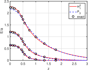

Refer to caption
(a) Su-Olson: P3 vs H12subscriptsuperscriptabsent21{}^{2}_{1}
Refer to caption
(b) Su-Olson: P5 vs H22subscriptsuperscriptabsent22{}^{2}_{2}
Refer to caption
(c) Su-Olson: P3 vs H12subscriptsuperscriptabsent21{}^{2}_{1} (log-log)
Refer to caption
(d) Su-Olson: P5 vs H22subscriptsuperscriptabsent22{}^{2}_{2} (log-log)
Figure 6: 4.3: Su-Olson problem) Three different simulations using HNTsubscriptsuperscriptabsent𝑇𝑁{}^{T}_{N} for the Su-Olson problem with Nz=100subscript𝑁𝑧100N_{z}=100, CFL=0.3CFL0.3\text{CFL}=0.3, and ctend=1.0, 3.16, 10𝑐subscript𝑡end1.03.1610ct_{\text{end}}=1.0,\,3.16,\,10, respectively. Panels (a) and (b) show P3, H21superscriptsubscriptabsent12{}_{1}^{2}, P5, and H22superscriptsubscriptabsent22{}_{2}^{2} on a linear scale, while panels (c) and (d) show those same solutions on a log-log scale.

4.4 Diffusive Marshak-wave problem

In this section, a diffusive Marshak-wave problem is investigated; this problem is a standard test case in the literature evans ; li ; mcclarren1 ; vikas . This problem consists of a semi-infinite medium of material with the opacity

σ=300/θ3.𝜎300superscript𝜃3\sigma=300/{\theta}^{3}. (91)

The computational domain is z[0.0,0.6]𝑧0.00.6z\in[0.0,0.6] and the initial conditions are given by the following with θ0=104subscript𝜃0superscript104{\theta}_{0}=10^{-4} keV:

I(t=0,z,μ)=12acθ04andθ(t=0,z)=θ0.formulae-sequence𝐼𝑡0𝑧𝜇12𝑎𝑐superscriptsubscript𝜃04and𝜃𝑡0𝑧subscript𝜃0I\left(t=0,z,\mu\right)=\frac{1}{2}ac{{\theta}_{0}}^{4}\qquad\text{and}\qquad{\theta}\left(t=0,z\right)={\theta}_{0}. (92)

We use the isotropic incoming boundary condition corresponding to a 1 keV temperature source on the left boundary zL=0subscript𝑧𝐿0z_{L}=0, and no incoming radiation on the right boundary at zR=0.6subscript𝑧𝑅0.6z_{R}=0.6:

I(t,zL,μ>0)=12acandI(t,zR,μ<0)=0.formulae-sequence𝐼𝑡subscript𝑧𝐿𝜇012𝑎𝑐and𝐼𝑡subscript𝑧𝑅𝜇00I\left(t,z_{L},\mu>0\right)=\frac{1}{2}ac\qquad\text{and}\qquad I\left(t,z_{R},\mu<0\right)=0. (93)

We compute the material temperature, θ(t,z)𝜃𝑡𝑧\theta(t,z) at various times: t=108𝑡superscript108t=10^{-8}s, 5×1085superscript1085\times 10^{-8}s, and 107superscript10710^{-7}s. In our numerical tests for this problem all HNTsubscriptsuperscriptabsent𝑇𝑁{}^{T}_{N} solutions look similar, thus, we only present H22subscriptsuperscriptabsent22{}^{2}_{2} solutions in Figure 7. In this test, we use Nz=16subscript𝑁𝑧16N_{z}=16 with the mesh size Δz=0.0375Δ𝑧0.0375\Delta{z}=0.0375. Despite the fact that we use a coarse mesh, the HNTsubscriptsuperscriptabsent𝑇𝑁{}^{T}_{N} solution is able to adequately capture the wave propagation front. Due to the fact that diffusion dominates, we are able to achieve stable results with a relaxed Courant number: CFL=1.7CFL1.7\text{CFL}=1.7. The reference solution shown in this plot is the semi-analytic equilibrium-diffusion solution (e.g., see mcclarren1 ).
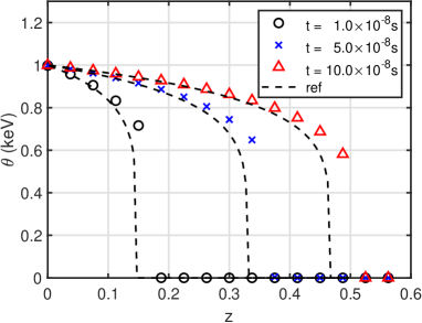
Refer to caption
Figure 7: 4.4: Diffusive Marshak-wave problem) The H22subscriptsuperscriptabsent22{}^{2}_{2} solutions for the material temperature, θ(t,z)𝜃𝑡𝑧\theta(t,z), for the diffusive Marshak-wave problem at various times: t=108𝑡superscript108t=10^{-8}s, 5×1085superscript1085\times 10^{-8}s, and 107superscript10710^{-7}s, respectively, with Nz=16subscript𝑁𝑧16N_{z}=16, σ=300/θ3𝜎300superscript𝜃3\sigma=300/{\theta}^{3}, θ0=104subscript𝜃0superscript104{\theta}_{0}=10^{-4} keV, and CFL=1.7CFL1.7\text{CFL}=1.7. The reference solution is the semi-analytic equilibrium-diffusion solution.

4.5 Marshak-wave in thin medium

Here we apply our scheme to a Marshak-wave problem in an optically thin medium with an opacity given by

σ=3/θ3.𝜎3superscript𝜃3\sigma=3/\theta^{3}. (94)

The radiation temperature is given by

θrad(t,z):=E(t,z)a4,assignsubscript𝜃rad𝑡𝑧4𝐸𝑡𝑧𝑎{\theta}_{\text{rad}}(t,z):=\sqrt[4]{\frac{E(t,z)}{a}}, (95)

and the computational domain is z[0,0.35]𝑧00.35z\in[0,0.35]. We use the isotropic incoming boundary condition corresponding to a 1 keV temperature source on the left boundary zL=0subscript𝑧𝐿0z_{L}=0, and no incoming radiation on the right boundary at zR=0.35subscript𝑧𝑅0.35z_{R}=0.35:

I(t,zL,μ>0)=12acandI(t,zR,μ<0)=0.formulae-sequence𝐼𝑡subscript𝑧𝐿𝜇012𝑎𝑐and𝐼𝑡subscript𝑧𝑅𝜇00I\left(t,z_{L},\mu>0\right)=\frac{1}{2}ac\qquad\text{and}\qquad I\left(t,z_{R},\mu<0\right)=0. (96)

The initial conditions are given by the following with θ0=105subscript𝜃0superscript105{\theta}_{0}=10^{-5} keV:

I(t=0,z,μ)=12acθ04andθ(t=0,z)=θ0.formulae-sequence𝐼𝑡0𝑧𝜇12𝑎𝑐superscriptsubscript𝜃04and𝜃𝑡0𝑧subscript𝜃0I\left(t=0,z,\mu\right)=\frac{1}{2}ac{{\theta}_{0}}^{4}\qquad\text{and}\qquad{\theta}\left(t=0,z\right)={\theta}_{0}. (97)

In Figure 8(a) we show the H22subscriptsuperscriptabsent22{}^{2}_{2} solution with Nz=400subscript𝑁𝑧400N_{z}=400 for the material temperature, θ𝜃\theta, and the radiation temperature, θradsubscript𝜃rad\theta_{\text{rad}} (95). In Figure 8(b) we show the material temperature error for H22subscriptsuperscriptabsent22{}^{2}_{2} for various Nzsubscript𝑁𝑧N_{z}. The error is computed by comparing the H22subscriptsuperscriptabsent22{}^{2}_{2} solutions with various Nzsubscript𝑁𝑧N_{z} to the P5 solution with Nz=2048subscript𝑁𝑧2048N_{z}=2048. This figure shows the expected degradation of the order of accuracy to first order in space for this problem due to the discontinuity of the solution.

Furthermore, in Figure 9 we investigate the various convergence rates of HN1,subscriptsuperscriptabsent1𝑁{}^{1}_{N},HN2subscriptsuperscriptabsent2𝑁{}^{2}_{N}, HN4subscriptsuperscriptabsent4𝑁{}^{4}_{N} and HN8subscriptsuperscriptabsent8𝑁{}^{8}_{N} with Nz=512subscript𝑁𝑧512N_{z}=512 as a function of N𝑁N. In particular, we compute the following approximate L2subscript𝐿2L_{2} error:

L2 error:=[0.35Nzi=1Nz(θ2j1T(tend,zi)θ99T(tend,zi))2]1/2,assignsubscript𝐿2 errorsuperscriptdelimited-[]0.35subscript𝑁𝑧superscriptsubscript𝑖1subscript𝑁𝑧superscriptsubscriptsuperscript𝜃𝑇2𝑗1subscript𝑡endsubscript𝑧𝑖subscriptsuperscript𝜃𝑇99subscript𝑡endsubscript𝑧𝑖212L_{2}\text{ error}\,:=\,\left[\frac{0.35}{N_{z}}\sum_{i=1}^{N_{z}}\Bigl{(}\theta^{T}_{2j-1}\left(t_{\text{end}},z_{i}\right)-\theta^{T}_{99}\left(t_{\text{end}},z_{i}\right)\Bigr{)}^{2}\right]^{1/2}, (98)

for j=1,2,,9𝑗129j=1,2,\ldots,9, where θNTsubscriptsuperscript𝜃𝑇𝑁\theta^{T}_{N} represents the material temperature as calculated with the HNTsubscriptsuperscriptabsent𝑇𝑁{}^{T}_{N} model. Due to the non-smoothness of the solution we note a fairly rapid convergence as a function of T𝑇T with fixed N𝑁N, and slower convergence as a function of N𝑁N with fixed T𝑇T.

Refer to caption
(a) The H22subscriptsuperscriptabsent22{}^{2}_{2} solutions with Nz=400subscript𝑁𝑧400N_{z}=400
Refer to caption
(b) H22subscriptsuperscriptabsent22{}^{2}_{2} convergence rate in position space
Figure 8: 4.5: Marshak-wave in thin medium) The H22subscriptsuperscriptabsent22{}^{2}_{2} solutions and convergence rate for the thin Marshak-wave problem at t=109𝑡superscript109t=10^{-9}s with σ=3/θ3𝜎3superscript𝜃3\sigma=3/{\theta}^{3}, θ0=105subscript𝜃0superscript105{\theta}_{0}=10^{-5} keV, and CFL=0.3CFL0.3\text{CFL}=0.3.
Refer to caption
Figure 9: 4.5: Marshak-wave in thin medium) Error in various HNTsubscriptsuperscriptabsent𝑇𝑁{}^{T}_{N} approximations with Nz=512subscript𝑁𝑧512N_{z}=512 and CFL=0.3CFL0.3\text{CFL}=0.3.

4.6 Smooth Marshak-wave

Finally, a smooth Marshak-wave problem is considered in this section to observe the convergence rate of our numerical scheme on a smooth solution in an optically thin medium. The opacity and radiation temperatures are again given by (94) and (95), respectively. Following lowrie ; mcclarren1 , the computational domain is z[0,0.8]𝑧00.8z\in[0,0.8] and the smooth initial conditions are given by:

I(t=0,z,μ)𝐼𝑡0𝑧𝜇\displaystyle I(t=0,z,\mu) =ac2[10.498(1+tanh[50(z0.25)])],absent𝑎𝑐2delimited-[]10.498150𝑧0.25\displaystyle=\frac{ac}{2}\biggl{[}1-0.498{\Bigl{(}1+\tanh{\bigl{[}50(z-0.25)\bigr{]}}\Bigr{)}}\biggr{]}, (99)
θ(t=0,z)𝜃𝑡0𝑧\displaystyle{\theta}(t=0,z) =(E(t=0,z)a)14.absentsuperscript𝐸𝑡0𝑧𝑎14\displaystyle=\left(\frac{E(t=0,z)}{a}\right)^{\frac{1}{4}}. (100)

The boundary conditions are given by

I(t,zL,μ>0)=I(t=0,zL,μ)andI(t,zR,μ<0)=0,formulae-sequence𝐼𝑡subscript𝑧𝐿𝜇0𝐼𝑡0subscript𝑧𝐿𝜇and𝐼𝑡subscript𝑧𝑅𝜇00I\left(t,z_{L},\mu>0\right)=I(t=0,z_{L},\mu)\qquad\text{and}\qquad I\left(t,z_{R},\mu<0\right)=0, (101)

where zL=0subscript𝑧𝐿0z_{L}=0 and zR=0.8subscript𝑧𝑅0.8z_{R}=0.8.

In Figure 10 we show the solution for the material temperature, θ(t,z)𝜃𝑡𝑧\theta(t,z), at various times: (a)

The initial condition for the material temperature, θ(t,z)𝜃𝑡𝑧\theta(t,z), is shown in Panel (a) of Figure 10. In Figure 10(b) we show a direct comparison of the material temperature as computed with P5subscript𝑃5P_{5} and H22subscriptsuperscript𝐻22H^{2}_{2}, both methods have DOF=6DOF6\text{DOF}=6, for Nz=128subscript𝑁𝑧128N_{z}=128. In Figure 10(c) and Figure 10(d) we show the material temperature as computed by P5subscript𝑃5P_{5} and H22subscriptsuperscript𝐻22H^{2}_{2} with various Nzsubscript𝑁𝑧N_{z}, respectively.

Refer to caption
(a) The initial condition
Refer to caption
(b) P5 vs H22subscriptsuperscriptabsent22{}^{2}_{2} with Nz=128subscript𝑁𝑧128N_{z}=128
Refer to caption
(c) P5 solutions with various Nzsubscript𝑁𝑧N_{z}
Refer to caption
(d) H22subscriptsuperscriptabsent22{}^{2}_{2} solutions with various Nzsubscript𝑁𝑧N_{z}
Figure 10: 4.6: Smooth Marshak-wave) Comparison of the P5 and HN2subscriptsuperscriptabsent2𝑁{}^{2}_{N} solutions for the material temperature for the smooth Marshak wave problem with CFL=0.3CFL0.3\text{CFL}=0.3.

Finally, in Figure 11 we demonstrate second-order convergence of the H22subscriptsuperscript𝐻22H^{2}_{2} with increasing mesh resolution Nzsubscript𝑁𝑧N_{z}. In this figure, the dashed-line indicates a slope of two on a log-log scale. In these convergence experiments the approximate L2subscript𝐿2L_{2} error is calculated via the formula:

L2(θθ2048):=0.8Nzk=1Nz(θkθk2048/(2m))2,assignsubscript𝐿2𝜃superscript𝜃20480.8subscript𝑁𝑧superscriptsubscript𝑘1subscript𝑁𝑧superscriptsubscript𝜃𝑘subscriptsuperscript𝜃2048superscript2𝑚𝑘2L_{2}({\theta}-{{\theta}}^{2048}):=\sqrt{\frac{0.8}{N_{z}}\sum_{k=1}^{N_{z}}{\left({\theta}_{k}-{{\theta}}^{2048/(2^{m})}_{k}\right)^{2}}}, (102)

where

θk2048/(2m+1)=12(θ2(k1)+12048/(2m)+θ2(k1)+22048/(2m)),subscriptsuperscript𝜃2048superscript2𝑚1𝑘12superscriptsubscript𝜃2𝑘112048superscript2𝑚superscriptsubscript𝜃2𝑘122048superscript2𝑚{{\theta}}^{2048/(2^{m+1})}_{k}=\frac{1}{2}\left({{\theta}}_{2(k-1)+1}^{2048/(2^{m})}+{{\theta}}_{2(k-1)+2}^{2048/(2^{m})}\right), (103)

for m=0,1,,7𝑚017m=0,1,\cdots,7. Here θ2048superscript𝜃2048{{\theta}}^{2048} represents the reference temperature solution on mesh with Nz=2048subscript𝑁𝑧2048N_{z}=2048 cells, and the superscript k𝑘k stands for the kthsuperscript𝑘thk^{\text{th}} grid cell. The idea encapsulated in formulas (102) and (103) is that we project the reference solution θ2048superscript𝜃2048{\theta}^{2048} onto coarser mesh, i.e., Nz=2048/(2m)subscript𝑁𝑧2048superscript2𝑚N_{z}=2048/(2^{m}), for m=1,2,,8𝑚128m=1,2,\cdots,8 by taking the average of left and right cell on finer mesh, to obtain θ1024,θ512,,θ8superscript𝜃1024superscript𝜃512superscript𝜃8{\theta}^{1024},{\theta}^{512},\cdots,{\theta}^{8}; once we have projected this solution down to the mesh on which θ𝜃\theta is defined, we can directly compute the L2subscript𝐿2L_{2} distance. In Figure 11 we have used this strategy with Nz=8subscript𝑁𝑧8N_{z}=8, 16, 32, 64, 128, 256, 512, and 1024 to show the convergence rate.
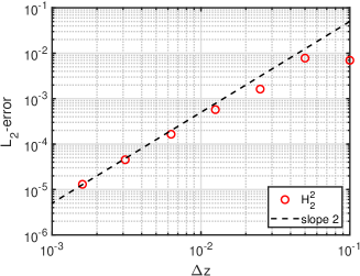
Refer to caption
Figure 11: 4.6: Smooth Marshak-wave) Convergence rate of the material temperature θ𝜃{\theta} for the smooth Marshak wave problem.

5 Conclusion

In this work we have developed the hybrid discrete (HNTsubscriptsuperscriptabsent𝑇𝑁{}^{T}_{N}) approximation method for the thermal radiative transfer (TRT) equations, and implemented a numerical discretization of these equations using a second order discontinuous Galerkin finite element method in conjunction with a semi-implicit time-stepping scheme. The HNTsubscriptsuperscriptabsent𝑇𝑁{}^{T}_{N} approach acquires desirable properties of two classical methods for the TRT equations, namely PN (spherical harmonics) and SN (discrete ordinates), and indeed reduces to each of these approximations in various limits: HN1subscriptsuperscriptabsent1𝑁{}^{1}_{N} \equiv PN and H0Tsubscriptsuperscriptabsent𝑇0{}^{T}_{0} \equiv ST. We proved that the HNTsubscriptsuperscriptabsent𝑇𝑁{}^{T}_{N} approximation results in a system of hyperbolic partial differential equations for all T1𝑇1T\geq 1 and N0𝑁0N\geq 0. In particular, in one spatial dimension, the HNTsubscriptsuperscriptabsent𝑇𝑁{}^{T}_{N} scheme is essentially a collection of PN approximations localized in each velocity band. Because of this structure, HNTsubscriptsuperscriptabsent𝑇𝑁{}^{T}_{N}, just like PN, can exhibit negative densities. However, because HNTsubscriptsuperscriptabsent𝑇𝑁{}^{T}_{N} has band-localized structure, we are able to control unphysical numerical oscillations by increasing the number of discrete regions in velocity space, thereby blending properties of PN and SN.

Once the HNTsubscriptsuperscriptabsent𝑇𝑁{}^{T}_{N} approximation was developed for TRT, we introduced a semi-implicit numerical method that is based on a second order explicit Runge-Kutta scheme for the the streaming term and an implicit Euler scheme for the material coupling term. Furthermore, in order to solve the material energy equation implicitly after each predictor and corrector step, we linearized the temperature term using a Taylor expansion; this avoided the need for an iterative procedure, and therefore improved efficiency. In order to reduce unphysical oscillation, we applied a slope limiter after each time step.

In the numerical results section we compared the solutions of the HNTsubscriptsuperscriptabsent𝑇𝑁{}^{T}_{N} and PN schemes for the various benchmark problems. We demonstrated for a variety of problems that for a fixed total number of moments, we are able to achieve accuracy gains over the PNHN1subscriptP𝑁subscriptsuperscriptH1𝑁\text{P}_{N}\equiv\text{H}^{1}_{N} approximation by balancing T𝑇T and N𝑁N. With a more balanced choice of T𝑇T and N𝑁N, HNTsubscriptsuperscriptabsent𝑇𝑁{}^{T}_{N} shows less oscillation than PN, especially in the presence of discontinuities. One may use the large T𝑇T when the problems include strong shocks or the solutions are non-smooth. Otherwise, one can use high N𝑁N instead. The control of the variables T𝑇T and N𝑁N can compensate for the shortcomings of PN and SN schemes.

In future work, we will develop extensions of the HTNsuperscriptsubscriptabsent𝑁𝑇{}_{N}^{T} method for multi-energy group models or frequency-dependent equations in multiple dimensions. In particular, just as we have done in this work, we will investigate various choices of N𝑁N and T𝑇T to achieve accurate and efficient moment closure in the multidimensional setting. We will also investigate adaptive strategies for selecting T𝑇T and N𝑁N in the presence of some appropriate error indicator.

Acknowledgements.
JAR was supported in part by NSF Grants DMS–1620128 and DMS–2012699.

References

  • (1) Adams, M.P., Adams, M.L., Hawkins, W.D., Smith, T., Rauchwerger, L., Amato, N.M., Bailey, T.S., Falgout, R.D., Kunen, A., Brown, P.: Provably optimal parallel transport sweeps on semi-structured grids. J. Comput. Phys. 407, 109–234 (2020)
  • (2) Brunner, T.A., Holloway, J.P.: Two-dimensional time-dependent Riemann solvers for neutron transport. J. Comput. Phys. 210(1), 386–399 (2005)
  • (3) Carlson, B.: Solution of the transport equation by the SN method. Los Alamos National Laboratory (1955)
  • (4) Carlson, B.: Tables of symmetric equal weight quadrature EQn over the unit sphere. Los Alamos National Laboratory (1971)
  • (5) Cohen, A.: An algebraic approach to certain differential eigenvalue problems. Linear Algebra Appl. 240, 183–198 (1996)
  • (6) Dubroca, B., Feugeas, J.L.: Etude théorique et numérique d’une hiérarchie de modèles aux moments pour le transfert radiatif. Comptes Rendus de l’Académie des Sciences-Series I-Mathematics 329(10), 915–920 (1999)
  • (7) Evans, T.M., Urbatsch, T.J., Lichtenstein, H., Morel, J.E.: A residual Monte Carlo method for discrete thermal radiative diffusion. J. Comput. Phys. 189(2), 539–556 (2003)
  • (8) Fan, Y.W., Li, R., Zheng, L.C.: A Nonlinear Moment Model for Radiative Transfer Equation in Slab Geometry. J. Comput. Phys. 404, 109–128 (2020)
  • (9) Fleck, J.A., Jr., Cummings, J.D.: An implicit Monte Carlo scheme for calculating time and frequency dependent nonlinear radiation transport. J. Comput. Phys. 8(3), 313–342 (1971)
  • (10) Gustafsson, B., Kreiss, H.O., Oliger, J.: Time-Dependent Problems and Difference Methods, 2nd Edition. Wiley, New York, United States (2013)
  • (11) Hauck, C., McClarren, R.: Positive p_n closures. SIAM Journal on Scientific Computing 32(5), 2603–2626 (2010)
  • (12) Hauck, C.D.: High-order entropy-based closures for linear transport in slab geometry. Communications in Mathematical Sciences 9(1), 187–205 (2011)
  • (13) Hauck, C.D., McClarren, R.G.: Positive PN closures. SIAM J. Sci. Comput. 32(5), 2603–2626 (2010)
  • (14) J. Lorenz, H.J.S.: Stiff well-posedness for hyperbolic systems with large relaxation terms (linear constant-coefficient problems). Adv. Differ. Equ. 2(4), 643–666 (1997)
  • (15) Jarrell, J., Adams, M.: Discrete-ordinates quadrature sets based on linear discontinuous finite elements. In: Proc. International Conference on Mathematics and Computational Methods applied to Nuclear Science and Engineering, Rio de Janeiro, Brazil (2011)
  • (16) Klar, A.: An asymptotic-induced scheme for nonstationary transport equations in the diffusive limit. SIAM J. Numer. Anal. 35(3), 1073–1094 (1998)
  • (17) Klar, A., Unterreiter, A.: Uniform stability of a finite difference scheme for transport equations in diffusive regimes. SIAM J. Numer. Anal. 40(3), 891–913 (2002)
  • (18) Koch, R., Krebs, W., Wittig, S., Viskanta, R.: The discrete ordinate quadrature schemes for multidimensional radiative transfer. J. Quant. Spectrosc. Ra. 53(4), 353–372 (1995)
  • (19) Laiu, M.P., Hauck, C.D., McClarren, R.G., O’Leary, D.P., Tits, A.L.: Positive filtered PN moment closures for linear kinetic equations. SIAM J. Numer. Anal. 54(6), 3214–3238 (2016)
  • (20) Larsen, E., Pomraning, G., Badham, V.: Asymptotic analysis of radiative transfer equations. J. Quant. Spectros. Radiat. Transf. 29(4), 285–310 (1983)
  • (21) Lathrop, K.D.: Ray effects in discrete ordinates equations. Nucl. Sci. Eng. 32(3), 357–369 (1968)
  • (22) Lathrop, K.D.: Remedies for ray effects. Nucl. Sci. Eng. 45(3), 255–268 (1971)
  • (23) Lathrop, K.D., Carlson, B.G.: Discrete ordinates angular quadrature of the neutron transport equation. Los Alamos Scientific Laboratory Report 3186 (1965)
  • (24) Lau, C., Adams, M.: Discrete Ordinates Quadratures Based on Linear and Quadratic Discontinuous Finite Elements over Spherical Quadrilaterals. Nucl. Sci. Eng. 185(1), 36–52 (2017)
  • (25) Lewis, E.E., Miller, W.F.: Computational Methods of Neutron Transport. John Wiley & Sons, DeKalb (1994)
  • (26) Li, W., Liu, C., Zhu, Y., Zhang, J., Xu, K.: Unified gas-kinetic wave-particle methods III: Multiscale photon transport. J. Comput. Phys. 408, 109–280 (2020)
  • (27) Lowrie, R.B.: A Comparison of Implicit Time Integration Methods for Nonlinear Relaxation and Diffusion. J. Comput. Phys. 196(2), 566–590 (2004)
  • (28) McClarren, R.G., Evans, T.M., Lowrie, R.B., Densmore, J.D.: Semi-implicit time integration for PN thermal radiative transfer. J. Comput. Phys. 227(16), 7561–7586 (2008)
  • (29) McClarren, R.G., Holloway, J.P., Brunner, T.A.: On solutions to the pn equations for thermal radiative transfer. Journal of Computational Physics 227(5), 2864–2885 (2008)
  • (30) Mcclarren, R.G., Lowrie, R.B.: The effects of slope limiting on asymptotic-preserving numerical methods for hyperbolic conservation laws. J. Comput. Phys. 227(23), 9711–9726 (2008)
  • (31) McClarren, R.G., Urbatsch, T.J.: A modified implicit monte carlo method for time-dependent radiative transfer with adaptive material coupling. Journal of Computational Physics 228(16), 5669–5686 (2009)
  • (32) Olson, G.: Second-order time evolution of P N equations for radiation transport. J. Comput. Phys. 228(8), 3072–3083 (2009)
  • (33) Olson, G.L., Auer, L.H., Hall, M.L.: Diffusion, p1, and other approximate forms of radiation transport. J. Quant. Spectrosc. Ra. 64(6), 619–634 (2000)
  • (34) Parlett, B.N.: The Symmetric Eigenvalue Problem. Prentice-Hall Series in Comput. Math. 61(7), 277–348 (1981)
  • (35) Pomraning, G.C.: Variational boundary conditions for the spherical harmonics approximation to the neutron transport equation. Ann. Phys. 27, 193–215 (1964)
  • (36) Pomraning, G.C.: The Equations of Radiation Hydrodynamics. Pergamon Press, Oxford, U.K. (1973)
  • (37) Shin, M.: Hybrid discrete (HNTsubscriptsuperscriptabsent𝑇𝑁{}^{T}_{N}) approximations to the equation of radiative transfer. Ph.D. thesis, Iowa State University, Ames, IA (2019)
  • (38) Siegel, R., Howell, J.R.: Thermal radiation heat transfer, vol. 3. Hemisphere Publishing Corp., Washington, United States (1972)
  • (39) Su, B., Olson, G.L.: An analytical benchmark for non-equilibrium radiative transfer in an isotropically scattering medium. Ann. Nucl. Energy 24(13), 1035–1055 (1997)
  • (40) Thurgood, C.P., Pollard, A., Becker, H.A.: The TN Quadrature Set for the Discrete Ordinates Method. J. Heat Transfer 117(4), 1068–1070 (1995)
  • (41) Vikas, V., Hauck, C., Wang, Z., Fox, R.: Radiation transport modeling using extended quadrature method of moments. J. Comput. Phys. 246(1), 221–241 (2013)
  • (42) Wikipedia: Gaussian quadrature (2021). URL https://en.wikipedia.org/wiki/Gaussian_quadrature
  • (43) Wollaber, A.B.: Four decades of implicit monte carlo. Journal of Computational and Theoretical Transport 45(1-2), 1–70 (2016)
  • (44) Zheng, W., McClarren, R.G.: Moment closures based on minimizing the residual of the pn angular expansion in radiation transport. Journal of Computational Physics 314, 682–699 (2016)