Deep NMF Topic Modeling

Abstract

Nonnegative matrix factorization (NMF) based topic modeling methods do not rely on model- or data-assumptions much. However, they are usually formulated as difficult optimization problems, which may suffer from bad local minima and high computational complexity. In this paper, we propose a deep NMF (DNMF) topic modeling framework to alleviate the aforementioned problems. It first applies an unsupervised deep learning method to learn latent hierarchical structures of documents, under the assumption that if we could learn a good representation of documents by, e.g. a deep model, then the topic word discovery problem can be boosted. Then, it takes the output of the deep model to constrain a topic-document distribution for the discovery of the discriminant topic words, which not only improves the efficacy but also reduces the computational complexity over conventional unsupervised NMF methods. We constrain the topic-document distribution in three ways, which takes the advantages of the three major sub-categories of NMF—basic NMF, structured NMF, and constrained NMF respectively. To overcome the weaknesses of deep neural networks in unsupervised topic modeling, we adopt a non-neural-network deep model—multilayer bootstrap network. To our knowledge, this is the first time that a deep NMF model is used for unsupervised topic modeling. We have compared the proposed method with a number of representative references covering major branches of topic modeling on a variety of real-world text corpora. Experimental results illustrate the effectiveness of the proposed method under various evaluation metrics.

1 Introduction

Topic modeling extracts salient features and discovers structural information from a large collection of documents [1]. This paper focuses on discussing the nonnative matrix factorization (NMF) based topic modeling [2, 3, 4, 5, 6, 7, 8]. NMF topic modeling usually decomposes the document-word representation of documents into a topic-document matrix and a word-topic matrix. Existing decomposition methods usually have the following two major problems. First, it is challenging to discover common patterns or topics in the documents and organize them into hierarchy [9, 10]. Second, the topic-word distribution do not meet human interpretation of documents [11, 12]. For example, traditional topic modeling may lose smaller subject codes, i.e. sub-topics, in the tails of large topics, which leads to the inability of describing topic dimensions in terms of the human interpretable objects of topics, and simultaneously loses all latent sub-structure within each topic [11]. Deep learning, which learns hierarchical data representations, provide one solution to the aforementioned problems. However, existing deep learning methods for topic modeling are mostly supervised, and fall into the category of probabilistic topic models [13, 14]. To our knowledge, unsupervised deep NMF topic modeling seems unexplored yet, due to maybe the high computational complexity of deep unsupervised NMF [15, 16] as well as the lack of supervised information of data.

1.1 Contributions

In this paper, we aim to explore an unsupervised deep NMF (DNMF) framework to address the above challenges. Because modeling topic hierarchies of documents and discovering topic words simultaneously is a complicated optimization problem, we propose to solve the two problems in sequence, under the assumption that, if the representation of documents is good enough, then the overall performance can be boosted [17]. The proposed method contains the following novelties:

• An unsupervised deep NMF framework is proposed. It first learns the topic hierarchies of documents by an unsupervised deep model, whose output is used to constrain the topic-document matrix. Then, it produces a good solution to the topic-document matrix and word-topic matrix by NMF under the constraint. It can have many implementations by incorporating different NMF methods and deep models. Unlike conventional NMF topic modeling methods that make predefined assumptions, DNMF alleviates the weaknesses of NMF, e.g. non-unique factorization, by deep learning. To our knowledge, this is the first work of unsupervised deep NMF for topic modeling.

• Three implementations of DNMF that reach the state-of-the-art performance are proposed. The three algorithms fall into the three major subclasses of NMF technologies [18], denoted as basic DNMF (bDNMF), strutured DNMF (sDNMF), and constrained DNMF (cDNMF) respectively. Specifically, bDNMF takes the output of the deep model as the topic-document matrix directly to generate the word-topic distribution. sDNMF takes the output of the deep model as the intrinsic geometry of the topic-document distribution, which is used to mask the topic-document matrix. cDNMF takes the output of the deep model as a regularization of the topic-document distribution. The convergence of the proposed algorithms is theoretically proved.

• Because the representation of documents in topic modeling is usually sparse and high-dimensional, existing deep neural networks can easily overfit to the documents. Although some methods reduce the dimension of the documents by discarding low-frequency words, their performance suffers from the compromise [19]. To address the problem, this paper applies multilayer bootstrap networks (MBN) to learn the topic hierarchies of documents. MBN contains three simple operators—random resampling, stacking, and one-nearest-neighbor optimization. To our knowledge, this is the first time that a non-neural-network unsupervised deep model is applied to topic modeling, which outperforms conventional shallow topic modeling methods significantly.

We have compared the proposed DNMF variants with 9 representative topic modeling methods [20, 1, 21, 22, 3, 5, 4, 23, 24] covering probabilistic topic models [20, 1, 21, 22], NMF methods [3, 5, 4, 23], and deep topic models [24]. Empirical results on the 20-newsgroups, topic detection and tracking database version 2 (TDT2), and Reuters-21578 corpora illustrate the effectiveness of DNMF in terms of three evaluation metrics. Moreover, the hyperparameters of the DNMF variants have stable working ranges across all situations, which facilitates their practical use.

In this paper, we first introduce some related work and preliminaries in the following two subsections, then present the proposed DNMF framework and its three implementations in Section 2. Section 3 presents the experimental results. Finally, Section 4 concludes our findings.

1.2 Related work

Probabilistic topic modeling: Topic models were originally formulated as unsupervised probabilistic models [1, 25, 26, 21]. A seminal work of probabilistic topic models is latent Dirichlet allocation (LDA) [1]. It models a document as a multinomial distribution over latent semantic topics, and models a topic itself as a multinomial distribution over words. The document-dependent topic embedding, governed by a Dirichlet prior, is estimated in an unsupervised way and then adopted as the low-dimensional feature for document classification and indexing. Later on, hierarchical tree-structured priors such as nested Dirichlet processing [25, 27] or nested Chinese restaurant process [28, 27] were applied to discover the hierarchy of topics and capture the nonlinearity of documents. However, the hierarchical probabilistic models suffer from conceptual and practical problems. For example, their optimization problem is NP-hard in the worst case due to the intractability of the posterior inference [29]. Existing methods have to resort to approximate inference methods, such as variational Bayes and Gibbs sampling which is also difficult to carry out [30]. Besides, because the exact inference is intractable, the models can never make predictions for words that are sharper than the distributions predicted by any of the individual topics. As a result, the hypothesis of probability distributions are unable to be applied to all text corpora [31]. Moreover, there is a lack of justification of the Bayesian priors as well [32]. Recently, a geometric Dirichlet means algorithm [33], which builds upon a weighted $k$-means clustering procedure and is augmented with a geometric correction, overcomes the computational and statistical inefficiencies encountered by probabilistic topic models based on Gibbs sampling and variational inference. However, the learned topic polytope is largely influenced by the performance of the clustering algorithm.

Deep probabilistic topic modeling: Another solution to the optimization difficulty of the hierarchical probabilistic models is to integrate the perspectives of the probabilistic models and deep neural networks. The integrated methods, named deep neural topic models, introduce neural network based priors as alternatives to Dirichlet process based priors [34, 35, 36, 37]. This integrates the powerfulness of neural network architecture into the inference of the probabilistic graph models, which makes the models not only interpretable but also powerful and easily extendable. However, they still fail to consider the veracity of the Bayesian hypothesis. The problem of component collapsing may also lead to bad local optima of the inference network in which all topics are identical.

NMF topic modeling: To deal with the optimization difficulty of the hierarchical probabilistic models, a large effort has been paid on polynomial time solvable topic modeling algorithms, many of which are formulated as separable nonnegative matrix factorization (NMF) methods [2, 3, 4, 5, 6, 7, 8]. They find the underlying parameters of topic models by decomposing the document-word data matrix into a weighted combination of a set of topic distributions [38]. A key problem in the context of NMF research is the separability issue, i.e., whether the matrix factors are unique [39]. When one applies NMF to topic modeling, the separability assumption is equivalent to an anchor-word assumption which assumes that every topic has a characteristic anchor word that does not appear in the other topics [3, 4, 5, 6]. However, because words and terms have multiple uses, the anchor word assumption may not always hold. How to avoid the unrealistic assumption is a key research topic. One solution explores tensor factorization models with three- or higher-order word co-occurence statistics. However, such statistics need many more samples than lower-order statistics to obtain reliable estimates, and separability still relies on additional assumptions [23], such as consecutive words being persistently drawn from the same topic. Another recent solution is anchor-free correlated topic modeling (AnchorFree) with second-order co-occurrence statistics. However, an assumption called sufficiently scattered condition is still needed to be made, though the assumption is much milder than the anchor-word assumption. Besides the problem of making additional assumptions to the data, NMF is also formulated as a shallow learning method with no more than one nonlinear layer, which may not capture the nonlinearity of documents and the hierarchy of topics well.

Deep NMF methods: The aforementioned NMF topic models are all shallow models, which is not powerful enough to grasp the nonlinearity of documents. In the NMF research community, a lot of efforts have been paid on the multilayered NMF algorithms with applications to image processing [40, 41], speech separation [42, 43], community detection [44], etc. The basic idea is to factorize a matrix into multiple factors, where the factorization can be either linear or nonlinear. If the factorization is nonlinear, then the method is called a deep NMF. For example, deep semi-NMF [15] factorizes the basis matrix into multiple factors with the optimization criterion of minimum reconstruction error, where it does not require the factorized weight matrix to be nonnegative anymore. Deep nonnegative basis matrix factorization [16] conducts deep factorization to the coefficient matrix with different regularization constraints on the basis matrix. However, because the bag-of-words representation of documents is high-dimensional and sparse, the application of the aforementioned idea to topic modeling is computationally high and may also suffer from overfitting. To our knowledge, no deep NMF topic modeling methods have been proposed yet.

Unsupervised deep learning for document clustering: Document clustering and topic modeling are two closely related tasks [17]. Unsupervised topic modeling projects documents into a topic embedding space, which promotes the development of document clustering. Recently, many works focused on learning the representations and topic assignments of documents simultaneously by deep neural networks [19, 45, 46, 47]. However, current deep learning methods for document clustering do not show advances over the shallow learning methods, such as NMF-based topic modeling. We conjecture that existing methods may not be good at dealing with sparse and high-dimensional representations of documents. As a compromise, they reduce the dimension of the sparse data by discarding the low-frequency words, which may significantly lose useful information. To deal with the aforementioned problems, here we develop deep models that are able to outperform conventional shallow models without discarding the low-frequency words. Note that, although some deep learning based topic models apply word embeddings to deep topic models [48, 49], it may not be unsuitable to compare them with the conventional topic modeling methods that work with the term frequency-inverse document frequency (TF-IDF) statistics.

1.3 Preliminaries

1.3.1 Notations

We first introduce some notations here. Regular letters, e.g. $\delta$, $M$, $t$, and $0$, indicate scalars. Bold lower-case letters, e.g. $\mathbf{d}$, indicate vectors. Bold capital letters, e.g. $\mathbf{D}$, $\mathbf{C}$, and $\mathbf{W}$, indicate matrices. The bold digit $\mathbf{0}$ indicates an all-zero vector or matrix. The operator ^T denotes the transpose. The notation $[\mathbf{C}]_{ij}$ indicates the elements of the matrix $\mathbf{C}$ at the $i$th column and $j$th row. The operator $\odot$ is the Hadamard multiplication. The operator $\mbox{Tr}(\cdot)$ denotes the trace of matrices.

1.3.2 Background

In topic modeling, given a corpus of $N$ documents with $K$ topics and a vocabulary of $V$ words, denoted as $\{\mathbf{d}_{n}\}_{n=1}^{N}$ where $\mathbf{d}_{n}=[d_{n,1},\ldots,d_{n,V}]^{T}$ with $d_{n,v}$ as the frequency of the $v$th word in the vocabulary that appears in the $n$th document. we aim to learn a topic-document matrix $\mathbf{W}=[w_{k,n}]\in\mathbb{R}_{+}^{K\times N}$ and a word-topic matrix $\mathbf{C}=[c_{v,k}]\in\mathbb{R}_{+}^{V\times K}$ from the document-word matrix $\mathbf{D}=[\mathbf{d}_{1},\ldots,\mathbf{d}_{N}]\in\mathbb{R}_{+}^{V\times N}$, where the notation $k\leq K$ is the topic index, $w_{k,n}$ is the topic label which describes the probability of the $n$th document belonging to the $k$th topic, and $c_{v,k}$ is the probability of the $v$th vocabulary that appears in the $k$th topic. The task of topic modeling is to find an approximate factorization:

$$\mathbf{D}\approx\mathbf{C}\mathbf{W}$$ (1)

NMF measures the distance between $\mathbf{D}$ and $\mathbf{C}\mathbf{W}$ by the squared Frobenius norm, and formulates the topic modeling problem as the following optimization problem:

$$(\mathbf{C},\mathbf{W})=\arg\min_{\mathbf{C}\geq\mathbf{0};\mathbf{W}\geq\mathbf{0}}\parallel{\mathbf{D}-\mathbf{C}\mathbf{W}}\parallel^{2}_{F}$$ (2)

where the nonnegative constraints make the solution interpretable. Under the anchor-word assumption, the word distribution $\mathbf{C}$ is enforced to be a block diagonal matrix, which guarantees a consistent solution [29, 50]. However, the anchor-word assumption is fragile in practice. Recently, many methods have been proposed to overcome this assumption [23, 51].

2 Deep NMF topic model

In this section, we first present the DNMF topic modeling framework in Section 2.1, then implements three DNMF topic modeling methods named bDNMF, cDNMF, and sDNMF respectively in Section 2.2, and finally introduce the unsupervised deep model in Section 2.3.

2.1 The framework of DNMF topic modeling

Traditional NMF topic modeling aims to learn a document representation by linear NMF essentially. In order to capture the manifold structure or topic hierarchies of documents, a natural way is to extend NMF into a deep NMF framework. Here we propose a DNMF framework which constrains the topic-document matrix by an unsupervised deep model with multiple layers of nonlinear transforms:

$$\begin{array}[]{c}\mathbf{D}\approx\mathbf{C}{\mathbf{W}}\\ \mbox{ subject to }\quad g({\mathbf{W}}|f(\mathbf{D}))\geq 0,\mbox{ }\mathbf{C}\geq 0,\mbox{ }{\mathbf{W}}\geq 0\end{array}$$ (3)

where $f(\cdot)$ is the unsupervised deep model and $g(\cdot)$ is a discriminator used to constrain ${\mathbf{W}}$ by $f(\cdot)$. $f(\cdot)$ performs like a prior that constrains the solution of ${\mathbf{W}}$ and $\mathbf{C}$ to be interpretable and discriminant, which is the fundamental difference between DNMF and conventional NMF topic models. The framework is illustrated in Fig. 1. It minimizes the reconstruction error between $\mathbf{D}$ and $\mathbf{C}\mathbf{W}$ in terms of the squared Frobenius norm.

A direct thought to solve problem (3) is to optimize $f({\mathbf{D}})$, $\mathbf{W}$, and $\mathbf{C}$ alternatively until convergence. However, it is too costly to train a deep model in a single iteration. In practice, we take the following optimization algorithm to solve problem (3):

• Pretrain $f({\mathbf{D}})$ first by an unsupervised deep model.

• Optimize ${\mathbf{W}}$ and $\mathbf{C}$ alternatively with $f(\mathbf{D})$ fixed until convergence.

The effectiveness of the above algorithm relies on the assumption that, if a high-quality $f(\mathbf{D})$ is obtained as a prior, then the solution of $\mathbf{C}$ and ${\mathbf{W}}$ is also boosted.

\begin{overpic}[width=184.9429pt]{DNMF1.pdf} \put(12.0,83.0){\normalsize${\color[rgb]{0,0,0}{\mathbf{W}}}$} \put(58.0,83.0){\normalsize${\color[rgb]{0,0,0}\mathbf{C}}$} \put(22.0,73.0){\small${\color[rgb]{0,0,0}\min\limits_{\mathbf{C}\geq 0}\frac{1}{2}\|\mathbf{D}-\mathbf{C}{\mathbf{W}}\|_{F}^{2}}$} \put(26.5,52.5){\normalsize${\color[rgb]{0,0,0}g({\mathbf{W}}|f(\mathbf{D}))}$} \put(40.0,45.0){\normalsize${\color[rgb]{0,0,0}f(\mathbf{D})}$} \put(40.0,-2.0){\normalsize${\color[rgb]{0,0,0}\mathbf{D}}$} \end{overpic}

Figure 1: The proposed DNMF framework.

The difference between the proposed topic modeling method and existing deep NMF methods [15, 16] is that the proposed method takes the deep model $f(\cdot)$ as an additional constraint of ${\mathbf{W}}$, while the methods in [15, 16] decomposes ${\mathbf{W}}$ directly into a hierarchical network. It is easy to see that the proposed framework can employ various unsupervised deep models to bring additional information into the matrix decomposition problem for specific applications. It is easy to constrain ${\mathbf{W}}$ flexibly as we will do in Section 2.2, which brings advanced NMF methods into the proposed framework. It also can either employ a pretrained deep model or conduct joint optimization of the deep model and the matrix decomposition. On the contrary, although [15, 16] can be applied to topic modeling, the computational complexity of their multilayered matrix decomposition is too high to be applied to topic modeling in practice. To our knowledge, they were not applied to topic modeling yet.

2.2 DNMF implementations

In this subsection, we first introduce three DNMF implementations that extend the three sub-categories of NMF [18] to their deep versions respectively, and then discuss the connection between the three implementations. Note that, besides the novelty of the DNMF framework, cDNMF and sDNMF are also fundamentally new even without the deep model $f({\mathbf{D}})$.

2.2.1 Basic DNMF topic modeling

Input :  Text corpus $\mathbf{D}$, the number of topics $T$, hyperparameters $\delta\geq 0$ and $M\geq 0$.

Output : $\mathbf{C}^{(t)}$, ${\mathbf{W}}$.

1 Initialize: topic-word distribution $\mathbf{C}^{0}$, $t\leftarrow 0$;

2 Construct a document-topic distribution $f(\mathbf{D})$ by deep unsupervised learning methods;

3 ${\mathbf{W}}\leftarrow f({\mathbf{D}})$;

4 repeat

5       Calculate $\mathbf{C}^{(t)}$ by (14);

6       $t\leftarrow t+1$;

7      

8until convergence;

Algorithm 1 bDNMF.

Many NMF topic modeling methods introduce polytope to interpret the geometry of documents [52, 53], i.e. $[\mathbf{D}]_{ij}=\sum_{k=1}^{K}[\mathbf{C}]_{ik}[\mathbf{W}]_{kj}$. A standard NMF topic modeling can always find an infinite solutions of ${\mathbf{C}}$ and ${\mathbf{W}}$ that satisfy ${\mathbf{D}}\approx{\mathbf{C}}{\mathbf{W}}$. To prevent such infinite solutions, various constraints have to be added. One of the simplest constraint is to provide one of the two factors beforehand, e.g. ${\mathbf{W}}$. However, it seems not easy to find a satisfied ${\mathbf{W}}$ beforehand in history. Fortunately, deep learning provides such an opportunity. We conjecture bravely that, if a good topic-document matrix ${\mathbf{W}}$ could be learned beforehand by deep learning, then the problem of finding the other factor ${\mathbf{C}}$ can be greatly simplified, which motivates bDNMF.

Given a latent document topic proportions $f(\mathbf{D})$ from a deep model, bDNMF interprets the documents by

$$[\mathbf{D}]_{ij}=\sum_{k=1}^{K}[\mathbf{C}]_{ik}[f(\mathbf{D})]_{kj}\mbox{ for }i=1,\dots,V;m=1,\dots,N.$$ (4)

It is a special case of the framework in Fig. 1 where $g(\cdot)$ is simply defined as $\mathbf{W}-f({\mathbf{D}})=\mathbf{0}$. Solving the factorization (4) in the NMF framework results in the following optimization problem:

$$\begin{split}\min\limits_{\mathbf{C}\geq\mathbf{0},f(\cdot)}D_{F}[\mathbf{D}||\mathbf{C}f(\mathbf{D})]\end{split}$$ (5)

where ${D}_{F}[\mathbf{D}||\mathbf{C}f(\mathbf{D})]$ denotes the Frobenius norm of NMF with $\mathbf{C}f(\mathbf{D})$ being an approximation of $\mathbf{D}$:

$$D_{{F}}[\mathbf{D}||\mathbf{C}f(\mathbf{D})]=\left\|\mathbf{D}-\mathbf{C}f(\mathbf{D})\right\|^{2}_{F}$$ (6)

We solve bDNMF in two steps. First, we generate the sparse representation of documents $f({\mathbf{D}})$ by a deep model. Then, problem (5) is formulated as a nonnegative least squares optimization problem, which can be solved by gradient descent algorithms or multiplicative update rules [54]. Here we prefer multiplicative update rules, since they do not have tunable hyperparameters. As we can see, when $f({\mathbf{D}})$ is given, problem (5) satisfies the following first-order Karush-Kuhn-Tucker (KKT) optimality conditions:

$$\left\{\begin{array}[]{ll}\mathbf{C}\geq\mathbf{0}\vspace{1ex}\\ \frac{\partial D_{F}(\mathbf{D}||\mathbf{C}f(\mathbf{D}))}{\partial\mathbf{C}}\geq\mathbf{0}\vspace{1ex}\\ \mathbf{C}\odot\frac{\partial D_{F}(\mathbf{D}||\mathbf{C}f(\mathbf{D}))}{\partial\mathbf{C}}=\mathbf{0}\end{array}\right.$$ (10)

which guarantees that the solution of (5) converges to a stationary point.

The multiplicative update rules are described as follows. Let $\Psi$ be the Lagrange multiplier of the constraint $\mathbf{C}\geq\mathbf{0}$, the Lagrangian $\mathcal{J}$ for (5) is

$$\begin{split}\mathcal{J}=&\mbox{Tr}(\mathbf{D}\mathbf{D}^{T})-2\mbox{Tr}(\mathbf{D}f(\mathbf{D})^{T}{\mathbf{C}}^{T})\\ &+\mbox{Tr}(\mathbf{C}f(\mathbf{D})f(\mathbf{D})^{T}{\mathbf{C}}^{T})+\mbox{Tr}(\mathbf{C}\mbox{\boldmath{$\Psi$}})\end{split}$$ (11)

The partial derivative of $\mathcal{J}$ with respect to $\mathbf{C}$ is

$$\begin{split}\frac{\partial\mathcal{J}}{\partial\mathbf{C}}=-2\mathbf{D}f(\mathbf{D})^{T}+2\mathbf{C}f(\mathbf{D})f(\mathbf{D})^{T}+\mbox{\boldmath{$\Psi$}}\end{split}$$ (12)

By the KKT condition $\mathbf{C}\odot\mbox{\boldmath{$\Psi$}}=\mathbf{0}$, we derive

$$2\mathbf{C}\odot(\mathbf{C}f(\mathbf{D})f(\mathbf{D})^{T})-2\mathbf{C}\odot(\mathbf{D}f(\mathbf{D})^{T})+\mathbf{C}\odot\mbox{\boldmath{$\Psi$}}=\mathbf{0}$$ (13)

Therefore, the multiplicative update rules for $\mathbf{C}$ can be inferred as follows:

$$\begin{split}[\mathbf{C}]^{(t+1)}_{ij}\leftarrow[\mathbf{C}]^{(t)}_{ij}\frac{[\mathbf{D}f(\mathbf{D})^{T}]_{ij}}{[\mathbf{C}f(\mathbf{D})f(\mathbf{D})^{T}]_{ij}}\end{split}$$ (14)

where the superscript ^(t) denotes the $t$th iteration of the multiplicative update rules.

bDNMF is summarized in Algorithm 1. It implements $g(\mathbf{W},f(\mathbf{D}))$ by simply setting $\mathbf{W}=f({\mathbf{D}})$. The main merit of bDNMF is that it can easily get the global optimum solution of ${\mathbf{C}}$ given ${\mathbf{W}}$ fixed, which avoids the non-unique solution of the NMF topic modeling in a simple way. Its effectiveness is largely affected by $f({\mathbf{D}})$. In practice, we implement $f(\mathbf{D})$ as semantic topic labels, which is obtained by the deep-learning-based document clustering.

2.2.2 Structured DNMF topic modeling

Although bDNMF is simple, it reduces NMF with only one variable when $f({\mathbf{D}})$ is given, which limits the flexibility of ${\mathbf{C}}$. To solve the problem, sDNMF modifies the regular factorization formulation (2) by a new discriminator ${\mathbf{W}}=f({\mathbf{D}})\odot\mathbf{T}$ instead of taking ${\mathbf{W}}=f({\mathbf{D}})$ where $\mathbf{T}$ is a new variable. Its objective function is formulated as follows:

$$\begin{split}\min\limits_{\mathbf{C}\geq\mathbf{0},\mathbf{T}\geq\mathbf{0},f(\cdot)}D_{F}(\mathbf{D}\|\mathbf{C}(f(\mathbf{D})\odot\mathbf{T}))\\ =\min\limits_{\mathbf{C}\geq\mathbf{0},\mathbf{T}\geq\mathbf{0},f(\cdot)}\|\mathbf{D}-\mathbf{C}(f(\mathbf{D})\odot\mathbf{T})\|_{F}^{2}\end{split}$$ (15)

Input :  Text corpus $\mathbf{D}$, the number of topics $T$, hyperparameters $\delta\geq 0$ and $M\geq 0$.

Output : $\mathbf{C}^{(t)}$, $f(\mathbf{D})$.

1 Initialize: topic-word distribution $\mathbf{C}^{0}$, document-topic distribution $\mathbf{T}^{0}$, weight matrix $\mathbf{T}^{0}$, $t\leftarrow 0$;

2 Construct a document-topic distribution $f(\mathbf{D})$ by deep unsupervised learning methods;

3 repeat

4       Calculate $\mathbf{T}^{(t)}$ by (25);

5       Calculate $\mathbf{C}^{(t)}$ by (26);

6       $t\leftarrow t+1$;

7      

8until convergence;

Algorithm 2 sDNMF.

Like bDNMF, we solve sDNMF by first generating $f({\mathbf{D}})$ by a deep model, which formulates problem (15) as an alternative least squares optimization problem. As we can see, when $f({\mathbf{D}})$ is given, problem (15) satisfies the following first-order KKT optimality conditions:

$$\left\{\begin{array}[]{ll}\mathbf{C}\geq\mathbf{0},\mathbf{T}\geq\mathbf{0}\vspace{1ex}\\ \frac{\partial{D_{F}(\mathbf{D}\|\mathbf{C}(f(\mathbf{D})\odot\mathbf{T}))}}{\partial\mathbf{C}}\geq\mathbf{0}\vspace{1ex}\\ \mathbf{C}\odot\frac{\partial{D_{F}(\mathbf{D}\|\mathbf{C}(f(\mathbf{D})\odot\mathbf{T}))}}{\partial\mathbf{C}}=\mathbf{0}\vspace{1ex}\\ \frac{\partial{D_{F}(\mathbf{D}\|\mathbf{C}(f(\mathbf{D})\odot\mathbf{T}))}}{\partial\mathbf{T}}\geq\mathbf{0}\vspace{1ex}\\ \mathbf{T}\odot\frac{\partial{D_{F}(\mathbf{D}\|\mathbf{C}(f(\mathbf{D})\odot\mathbf{T}))}}{\partial\mathbf{T}}=\mathbf{0}\vspace{1ex}\\ \end{array}\right.$$ (21)

which guarantees that the solution of (15) converges to a stationary point.

Let $\mathcal{\mathbf{U}}$ and $\mathcal{\mathbf{V}}$ denote the Lagrange multipliers of $\mathbf{C}$ and $\mathbf{T}$ respectively. Then, minimizing (15) is equivalent to minimizing the Lagrangian $\mathcal{J}$:

$$\begin{split}\mathcal{J}=D_{F}(\mathbf{D}\|\mathbf{C}\mathbf{T},f(\mathbf{D}))+\mbox{Tr}(\mathcal{\mathbf{U}}\mathbf{C}^{T})+\mbox{Tr}(\mathcal{\mathbf{V}}\mathbf{T}^{T})\end{split}$$ (22)

Taking partial derivatives in (22) derives

$$\begin{split}\frac{\partial\mathcal{J}}{\partial\mathbf{C}}=&2\mathbf{C}(f(\mathbf{D})\odot\mathbf{T})^{T}(f(\mathbf{D})\odot\mathbf{T})\\ &-2\mathbf{D}^{T}(f(\mathbf{D})\odot\mathbf{T})+\mathcal{\mathbf{U}}\end{split}$$ (23)

$$\begin{split}\frac{\partial\mathcal{J}}{\partial\mathbf{T}}=&2((f(\mathbf{D})\odot\mathbf{T})\mathbf{C}\mathbf{C}^{T})\odot f(\mathbf{D})\\ &-2(f(\mathbf{D})\odot\mathbf{D}\mathbf{C}^{T})+\mathcal{\mathbf{V}}\end{split}$$ (24)

Combining with the KKT conditions, we obtain the update rules:

$$\begin{split}[\mathbf{T}]^{(t+1)}_{ij}\leftarrow[\mathbf{T}]^{(t)}_{ij}\frac{[(\mathbf{D}\mathbf{C}^{T})\odot f(\mathbf{D})]_{ij}}{[((f(\mathbf{D})\odot\mathbf{T})\mathbf{C}\mathbf{C}^{T})\odot f(\mathbf{D})]_{ij}}\end{split}$$ (25)

$$\begin{split}[\mathbf{C}]^{(t+1)}_{ij}\leftarrow[\mathbf{C}]^{(t)}_{ij}\frac{[(f(\mathbf{D})\odot\mathbf{T})^{T}\mathbf{D}]_{ij}}{[(f(\mathbf{D})\odot\mathbf{T})^{T}(f(\mathbf{D})\odot\mathbf{T})\mathbf{C}]_{ij}}\end{split}$$ (26)

sDNMF is summarized in Algorithm 2. It promotes the effectiveness of ${\mathbf{C}}$ by introducing the internal variable $\mathbf{T}$ to bridge the gap between $f({\mathbf{D}})$ and ${\mathbf{C}}$.

2.2.3 Constrained DNMF topic modeling

Input :  Text corpus $\mathbf{D}$, number of topics $T$, hyperparameters $\delta\geq 0$, $M\geq 0$, $\lambda_{1}\geq 0$, and $\lambda_{2}\geq 0$.

Output : $\mathbf{C}^{(t)}$, $f(\mathbf{D})$.

1 Initialize: topic-word distribution $\mathbf{C}^{0}$, document-topic distribution ${\mathbf{W}}^{0}$, weight matrix $\mathbf{T}^{0}$, $t\leftarrow 0$;

2 Construct a document-topic distribution $f(\mathbf{D})$ by deep unsupervised learning methods;

3 repeat

4       Calculate $\mathbf{W}^{(t)}$ by (43);

5       Calculate $\mathbf{C}^{(t)}$ by (44);

6       Calculate $\mathbf{T}^{(t)}$ by (45);

7       $t\leftarrow t+1$;

8      

9until convergence;

Algorithm 3 cDNMF.

bDNMF and sDNMF intrinsically assumes that each document contains only one topic, which may not be true. To overcome the weakness of bDNMF and sDNMF, we propose cDNMF which introduces $f({\mathbf{D}})$ as a regularization on ${\mathbf{W}}$ instead of masking ${\mathbf{W}}$ by $f({\mathbf{D}})$ directly.

Specifically, we implement the discriminator $g({\mathbf{W}},f(\mathbf{D}))$ as a real-valued regression response of the semantic topic labels $f(\mathbf{D})$:

$$\begin{array}[]{c}\min\limits_{\mathbf{T}\in\mathbb{R}^{K\times K},{\mathbf{W}}\geq\mathbf{0}}\|f(\mathbf{D})-\mathbf{T}\mathbf{W}\|_{F}^{2}\end{array}$$ (27)

where $\mathbf{T}$ denotes a linear transform of ${\mathbf{W}}$. To further constrains the word-topic matrix $\mathbf{C}$ for highly meaningful topic words, we propose a word-word affinity regularization $\Omega(\mathbf{C})$:

$$\Omega(\mathbf{C})=\|\mathbf{C}\mathbf{C}^{T}-\mathbf{D}\mathbf{D}^{T}\|_{F}^{2}$$ (28)

which encodes the word-word semantics from the shared knowledge between the documents into $\mathbf{C}$. To our knowledge, this is the first time that such a regularization is introduced to the NMF topic modeling.

Substituting (27) and (28) into the DNMF framework derives the objective of cDNMF:

$$\min\limits_{\mathbf{T}\geq\mathbf{0},\mathbf{C}\geq\mathbf{0},\mathbf{W}\geq\mathbf{0},f(\cdot)}D_{F}(\mathbf{D}||\mathbf{C}{\mathbf{W}},\mathbf{T},f(\mathbf{D}))$$ (29)

where

$$\begin{array}[]{ll}D_{F}(\mathbf{D}||\mathbf{C}{\mathbf{W}},\mathbf{T},f(\mathbf{D}))\\ =\|\mathbf{D}-\mathbf{C}{\mathbf{W}}\|_{F}^{2}+\lambda_{1}\|f(\mathbf{D})-\mathbf{T}{\mathbf{W}}\|_{F}^{2}+\lambda_{2}\Omega(\mathbf{C})\\ \end{array}$$ (30)

with $\lambda_{1}$ and $\lambda_{2}$ as two hyperparameters.

Like bDNMF, we solve cDNMF by first obtaining $f({\mathbf{D}})$ from a deep model, and taking $f({\mathbf{D}})$ as a constant of (29). Then, we optimize (29) for $\mathbf{C}$, ${\mathbf{W}}$, and $\mathbf{T}$ by the alterative least squares optimization algorithm. When $f({\mathbf{D}})$ is given, problem (29) satisfies the following first-order KKT optimality conditions:

$$\left\{\begin{array}[]{ll}\mathbf{C}\geq\mathbf{0},\mathbf{W}\geq\mathbf{0},\mathbf{T}\geq\mathbf{0}\vspace{1ex}\\ \frac{\partial{D_{F}(\mathbf{D}||\mathbf{C}{\mathbf{W}},\mathbf{T},f(\mathbf{D}))}}{\partial\mathbf{C}}\geq\mathbf{0}\vspace{1ex}\\ \mathbf{C}\odot\frac{\partial{D_{F}(\mathbf{D}||\mathbf{C}{\mathbf{W}},\mathbf{T},f(\mathbf{D}))}}{\partial\mathbf{C}}=\mathbf{0}\vspace{1ex}\\ \frac{\partial{D_{F}(\mathbf{D}||\mathbf{C}{\mathbf{W}},\mathbf{T},f(\mathbf{D}))}}{\partial\mathbf{W}}\geq\mathbf{0}\vspace{1ex}\\ \mathbf{W}\odot\frac{\partial{D_{F}(\mathbf{D}||\mathbf{C}{\mathbf{W}},\mathbf{T},f(\mathbf{D}))}}{\partial\mathbf{W}}=\mathbf{0}\vspace{1ex}\\ \frac{\partial{D_{F}(\mathbf{D}||\mathbf{C}{\mathbf{W}},\mathbf{T},f(\mathbf{D}))}}{\partial\mathbf{T}}\geq\mathbf{0}\vspace{1ex}\\ \mathbf{T}\odot\frac{\partial{D_{F}(\mathbf{D}||\mathbf{C}{\mathbf{W}},\mathbf{T},f(\mathbf{D}))}}{\partial\mathbf{T}}=\mathbf{0}\vspace{1ex}\\ \end{array}\right.$$ (38)

which guarantees that the optimization of (29) converges to a stationary point. Let $\Psi$, ${\mathcal{\mathbf{Q}}}$, and $\mathcal{\mathbf{P}}$ be the Lagrange multipliers of the constraints $\mathbf{C}\geq\mathbf{0}$, $\mathbf{W}\geq\mathbf{0}$ and $\mathbf{T}\geq\mathbf{0}$, respectively. The Lagrangian $\mathcal{J}$ of (29) is

$$\begin{split}\mathcal{J}=&\mbox{Tr}(\mathbf{D}\mathbf{D}^{T})-2\mbox{Tr}(\mathbf{D}{\mathbf{W}}^{T}\mathbf{C}^{T})+\mbox{Tr}(\mathbf{C}{\mathbf{W}}{\mathbf{W}}^{T}\mathbf{C}^{T})\\ &+\lambda_{1}\mbox{Tr}(f(\mathbf{D})f^{T}(\mathbf{D}))-2\lambda_{1}\mbox{Tr}(f(\mathbf{D}){\mathbf{W}}^{T}\mathbf{T}^{T})\\ &+\lambda_{1}\mbox{Tr}(\mathbf{T}\mathbf{W}\mathbf{W}^{T}\mathbf{T}^{T})+\lambda_{2}\mbox{Tr}(\mathbf{D}\mathbf{D}^{T}\mathbf{D}\mathbf{D}^{T})\\ &-2\lambda_{2}\mbox{Tr}(\mathbf{D}\mathbf{D}^{T}\mathbf{C}\mathbf{C}^{T})+\lambda_{2}\mbox{Tr}(\mathbf{C}\mathbf{C}^{T}\mathbf{C}\mathbf{C}^{T})\\ &+\mbox{Tr}(\mathbf{C}\mbox{\boldmath{$\Psi$}})+\mbox{Tr}(\mathbf{W}\mathcal{\mathbf{Q}})+\mbox{Tr}(\mathbf{T}\mathcal{\mathbf{P}})\\ \end{split}$$ (39)

The partial derivatives of $\mathcal{J}$ with respect to $\mathbf{C}$, $\mathbf{W}$ and $\mathbf{T}$ are

$$\begin{split}\frac{\partial\mathcal{J}}{\partial\mathbf{C}}=&-2\mathbf{D}\mathbf{W}^{T}+2\mathbf{C}{\mathbf{W}}{\mathbf{W}}^{T}-4\lambda_{2}\mathbf{D}\mathbf{D}^{T}\mathbf{C}+\\ &4\lambda_{2}\mathbf{C}\mathbf{C}^{T}\mathbf{C}+\mbox{\boldmath{$\Psi$}}\end{split}$$ (40)

$$\begin{split}\frac{\partial\mathcal{J}}{\partial\mathbf{W}}=&-2\mathbf{C}^{T}\mathbf{D}+2\mathbf{C}^{T}\mathbf{C}{\mathbf{W}}-2\lambda_{1}\mathbf{T}^{T}f(\mathbf{D})+\\ &2\lambda_{1}\mathbf{T}^{T}\mathbf{T}{\mathbf{W}}+\mathcal{\mathbf{Q}}\end{split}$$ (41)

$$\begin{split}\frac{\partial\mathcal{J}}{\partial\mathbf{T}}=-2\lambda_{1}f(\mathbf{D})\mathbf{W}^{T}+2\lambda_{1}\mathbf{T}{\mathbf{W}}{\mathbf{W}}^{T}+\mathcal{\mathbf{P}}\end{split}$$ (42)

Using the KKT conditions $\mathbf{C}\odot\mbox{\boldmath{$\Psi$}}=\mathbf{0}$, $\mathbf{W}\odot\mathcal{\mathbf{Q}}=\mathbf{0}$ and $\mathbf{T}\odot\mathcal{\mathbf{P}}=\mathbf{0}$ we get the following update rule for $\mathbf{C}$:

$$\begin{split}[\mathbf{W}]^{(t+1)}_{ij}\leftarrow[\mathbf{W}]^{(t)}_{ij}\frac{[\mathbf{C}^{T}\mathbf{D}]_{ij}+\lambda_{1}[\mathbf{T}^{T}f(\mathbf{D})]_{ij}}{[\mathbf{C}^{T}\mathbf{C}{\mathbf{W}}]_{ij}+\lambda_{1}[\mathbf{T}^{T}\mathbf{T}\mathbf{W}]_{ij}}\end{split}$$ (43)

$$\begin{split}[\mathbf{C}]^{(t+1)}_{ij}\leftarrow[\mathbf{C}]^{(t)}_{ij}\frac{[\mathbf{D}\mathbf{W}^{T}]_{ij}+2\lambda_{2}[\mathbf{D}\mathbf{D}^{T}\mathbf{C}]_{ij}}{[\mathbf{C}{\mathbf{W}}{\mathbf{W}}^{T}]_{ij}+2\lambda_{2}[\mathbf{C}\mathbf{C}^{T}\mathbf{C}]_{ij}}\end{split}$$ (44)

$$\begin{split}[\mathbf{T}]^{(t+1)}_{ij}\leftarrow[\mathbf{T}]^{(t)}_{ij}\frac{[f(\mathbf{D})\mathbf{W}^{T}]_{ij}}{[\mathbf{T}{\mathbf{W}}{\mathbf{W}}^{T}]_{ij}}\end{split}$$ (45)

cDNMF is summarized in Algorithm 3. Its merit over bDNMF and sDNMF is that cDNMF avoids the assumption that each document contains only one topic. However, it has two tunable hyperparameters. As we know, there is no way to tune the hyperparameters in unsupervised topic modeling. To remedy this weakness, we take the document clustering result $f({\mathbf{D}})$ as the pseudo labels for tuning the hyperparameters.

2.3 Deep unsupervised document clustering

In Section 1.2, we have summarized the recent progress of unsupervised deep learning methods for document clustering. To our knowledge, the advantage of the deep learning based document clustering over conventional document clustering methods is not apparent in general. In this section, we propose a novel unsupervised deep learning based document clustering method, named MBN, to address this issue.

2.3.1 Algorithm description of MBN

MBN consists of $L$ gradually narrowed hidden layers from bottom-up. Each hidden layer consists of $M$ $k$-centroids clusterings ($M\gg 1$), where parameter $k$ at the $l$-th layer is denoted by $k_{l}$, $l=1,\ldots,L$. Each $k_{l}$-centroids clustering has $k_{l}$ output units, each of which indicates one cluster. The output layer is linear-kernel-based spectral clustering [55]. We take the output of the spectral clustering as $f({\mathbf{D}})$.

MBN is trained simply by stacking. To train the $l$-th layer, we simply train each $k_{l}$-centroids clustering as follows:

• Random sampling of input. The first step randomly selects $k_{l}$ documents from ${\mathbf{X}^{(l-1)}=[\mathbf{x}_{1}^{(l-1)},\ldots,\mathbf{x}_{N}^{(l-1)}]}$ as the $k_{l}$ centroids of the clustering. If $l=1$, then ${\mathbf{X}^{(l-1)}=\textbf{D}}$.

• One-nearest-neighbor learning. The second step assigns an input document $\mathbf{x}^{(l-1)}$ to one of the $k_{l}$ clusters by one-nearest-neighbor learning, and outputs a $k_{l}$-dimensional indicator vector ${\textbf{h}=[h_{1},\dots,h_{k_{l}}]^{T}}$, which is a one-hot sparse vector indicating the nearest centroid to $\mathbf{x}^{(l-1)}$.

The output units of all $k_{l}$-centroids clusterings are concatenated as the input of their upper layer, i.e. $\mathbf{x}^{(l)}=[\mathbf{h}_{1}^{T},\ldots,\mathbf{h}_{M}^{T}]^{T}$. We use cosine similarity to evaluate the similarity between the input and the centroids in all layers.

As described in [56], each layer of MBN is a histogram-based nonparametric density estimator, which does not make model assumptions on data; the hierarchical structure of MBN captures the nonlinearity of documents by building a vast number of hierarchical trees on the TF-IDF feature space implicitly.

2.3.2 Network structure of MBN

The network structure of MBN is important to its effectiveness. First of all, we should set the hyperparameter $M$ to a large number, which guarantees the high estimation accuracy of MBN at each layer. Then, to maintain the tree structure and discriminability of MBN, we should set $\{k_{l}\}_{l=1}^{L}$ carefully by the following criteria:

$$k_{1}=\left\lfloor N/2\right\rfloor,\quad k_{l}=\left\lfloor\delta k_{l-1}\right\rfloor$$ (46)

$$\begin{array}[]{l}k_{L}\mbox{ is set to guarantee that at least a document per}\\ \mbox{class is chosen by a random sample in probability}\end{array}$$ (47)

where $\delta\in[0,1)$ is a user defined hyperparameter with $0.5$ as the default.

As analyzed in [56], the hyperparameter $\delta$ controls how aggressively the nonlinearity of data is reduced. If the data is highly nonlinear, then we set $\delta$ to a large number, which results in a very deep architecture; otherwise, we set $\delta$ to a small number. MBN is relatively sensitive to the selection of $\delta$. As will be shown in the experiment, setting $\delta=0.5$ is safe, though tuning $\delta$ may lead to better performance.

The criterion (47) guarantees that each $k_{L}$-centroids clustering is a valid one in probability. Specifically, for any $k_{L}$-centroids clustering, if its centroids do not contain any document of a topic, then its output representation has no discriminability to the topic. To understand this point, we consider an extreme case: if $k_{L}=1$, then the top hidden layer of MBN outputs the same representation for all documents. In practice, we implement (47) by:

$$k_{L}\approx\left\{\begin{array}[]{ll}30\lceil\frac{N}{N_{z}}\rceil,&\mbox{if $\mathbf{D}$ is strongly class imbalanced}\\ 1.5K,&\mbox{otherwise}\\ \end{array}\right.$$ (50)

where $N_{z}$ is the size of the smallest topic. If $N_{z}$ is unknown, we simply set $k_{L}$ to a number that is significantly larger than the number of topics, e.g. 300 or so.

2.4 Discussions

The DNMF variants are new in the NMF study even without the deep model. First, the structured NMF component of sDNMF is different from existing structured NMF models. For example, nonsmooth NMF [57] incorporates a smooth factor to make the basis matrix and coefficient matrix (i.e. the topic-document matrix and word-topic matrix respectively in topic modeling) sparse, and reconciles the contradiction between approximation and sparseness. Some other structured NMF methods [58, 59] adopt a global centroid for each basis vector to capture the manifold structure. However, sDNMF takes the sparse representation of documents as a mask of the basis matrix. Second, although it is common to add regularization terms into the objective function of NMF, we did not observe the term (28) in the study of NMF. Although some similar form to (27) has been proposed in [60] for hyperspectral unmixing, they learn the representation of data by a shallow model. Therefore, the objective function of cDNMF is fundamentally new to our knowledge.

Because sDNMF and cDNMF are non-convex optimization problems, we take the alternative iterative optimization algorithm to solve them. The convergence of the algorithm is guaranteed by the following theorem:

Theorem 1.

The objective values of sDNMF and cDNMF decreases monotonically and converges to a stationary point.

Proof.

See Appendix A for the proof of Theorem 1 where we take cDNMF as an example. The proof can be applied to sDNMF too whose objective value is non-increasing under the update rules (26) and (25). ∎

3 Experiments

In this section, we compare the proposed DNMF with nine topic modeling methods on three benchmark text datasets.

3.1 Data sets

We conducted experiments on the 20-newsrgoups, top 30 largest topics of TDT2, and top 30 largest topics of Reuters-21578 document corpora. 20-Newsgroups consists of 18,846 documents with a vocabulary size of 26,214. This data set has 20 categories, each of which contains around 1,000 documents. The top 30 largest topics of TDT2 consists of 9,394 documents with a vocabulary size of 36,771 words. The top 30 largest topics of Reuters-21578 contains 8,293 documents in total with a vocabulary size of 18,933 words.

For TDT2 and Reuter-21578, we randomly selected 3 to 25 topics from the top 30 largest topics respectively for evaluation. For 20-newsgroups, we randomly selected 3 to 20 topics respectively for evaluation. For each comparison, we reported the average results over 50 Monte-Carlo runs. The indices of the topics of the 50 independent runs on TDT2 are the same as those at http://www.cad.zju.edu.cn/home/dengcai/Data/TextData.html. We extracted TF-IDF statistics from the bag-of-words model of the documents, and took cosine similarity to measure the similarity of two documents in the TF-IDF space.

3.2 Comparison algorithms

The hyperparameters of DNMF in all experiments were set as follows: $M=400$, $\delta=0.5$, $\lambda_{1}=1$, and $\lambda_{2}=1$, unless otherwise stated. We compared DNMF with four probabilistic models [20, 1, 21, 22], four NMF methods [3, 5, 4, 23], and one deep learning based topic model [24] with their optimal hyperparameter settings. They are listed as follows:

• Probabilistic latent semantic indexing (PLSI)[20].

• Latent Dirichlet allocation (LDA)[1].

• Laplacian probabilistic latent semantic indexing (LapPLSI)[21].

• Locally-consistent topic modeling (LTM) [22].

• Successive projection algorithm (SPA)[3].

• Successive nonnegative projection (SNPA) [5].

• A fast conical hull algorithm (XRAY)[4].

• Anchor-free correlated topic modeling (AchorFree) [23].

• Deep Poisson factor modeling (DPFA) [24]: it is a deep learning based topic model built on the Dirichlet process. We set its DNN to a depth of two hidden layers, and set the number of the hidden units of the two hidden layers to $K$ and $\lceil K/2\rceil$ respectively. We used the output from the first hidden layer for clustering. The above setting results in the best performance.

3.3 Evaluation Metrics

We evaluated the comparison results in terms of clustering accuracy (ACC), coherence, and similarity count (SimCount). Clustering accuracy applies the hungarian algorithm to solve the permutation problem of predicted labels. Coherence evaluates the quality of a single topic by finding how many topic words belonging to the topic appear across the documents of the topic [50]:

$${\rm{Coh}}(\nu)=\sum_{v_{1},v_{2}\in{\nu}}\log{\frac{{\rm{freq}}(v_{1},v_{2})+\varepsilon}{{\rm{freq}}(v_{2})}}$$ (51)

where $v_{1}$ and $v_{2}$ denote two words in the vocabulary, ${\rm{freq}}(v_{1},v_{2})$ denotes the number of the documents where $v_{1}$ and $v_{2}$ co-appear, ${\rm{freq}}(v_{2})$ denotes the number of the documents containing $v_{2}$, and $\varepsilon=0.01$ is used to prevent the input of the logarithm operator from zero. The higher the clustering accuracy or coherence score is, the better the topic model is. Because the coherence measurement does not evaluate the redundancy of a topic, we used similarity count to measure the similarity between the topics. For each topic, similarity count is obtained simply by counting the number of the overlapped words in the leading $K$ words. The lower the similarity count score is, the better the topic model is.

3.4 Main results

Figure 2: Visualizations of 20Newsgroups produced by DNMF.

TABLE I: Topic words discovered by bDNMF and AnchorFree on a 5-topic subset of TDT2 corpus. The topic words in bold denotes overlapped words between topics.

AnchorFree					bDNMF
Topic 1	Topic 2	Topic 3	Topic 4	Topic 5	Topic 1	Topic 2	Topic 3	Topic 4	Topic 5
netanyahu	asian	bowl	tornadoes	economic	netanyahu	asian	bowl	florida	nigeria
israeli	asia	super	florida	indonesia	israeli	percent	super	tornadoes	abacha
israel	economic	broncos	central	asian	israel	indonesia	broncos	tornado	military
palestinian	financial	denver	storms	financial	palestinian	asia	denver	storms	police
peace	percent	packers	ripped	imf	peace	economy	packers	killed	nigerian
arafat	economy	bay	victims	economy	albright	financial	green	victims	opposition
palestinians	market	green	tornado	crisis	arafat	market	game	damage	nigerias
albright	stock	football	homes	asia	palestinians	stock	bay	homes	anti
benjamin	crisis	game	killed	monetary	talks	economic	football	ripped	elections
west	markets	san	people	currency	west	billion	elway	nino	arrested
talks	stocks	elway	damage	billion	benjamin	crisis	san	el	lagos
bank	currency	diego	twisters	fund	madeleine	imf	team	weather	democracy
prime	prices	xxxii	nino	percent	london	japan	sports	twisters	sani
london	dollar	nfl	el	international	ross	spkr	diego	storm	sysciviliantem
minister	investors	quarterback	deadly	government	withdrawal	currency	coach	rain	protest
yasser	index	sports	storm	bank	process	markets	play	stories	protests
ross	billion	play	counties	korea	prime	dollar	win	deadly	presidential
withdrawal	bank	yards	weather	south	yasser	south	teams	struck	abachas
madeleine	growth	favre	funerals	indonesian	secretary	government	season	residents	violent
13	indonesia	pittsburgh	toll	suharto	13	prices	fans	california	nigerians

TABLE II: Performance of the comparison algorithms on 20-newsgroups.

	#topics	PLSI	LDA	LapPLSI	LTM	SPA	SNPA	XRAY	AnchorFree	DFPA	bDNMF	sDNMF	cDNMF
ACC	3	0.4243	0.8134	0.7596	0.8955	0.4279	0.4275	0.4086	0.8763	0.8402	0.9101	0.9101	0.9101
	4	0.3671	0.7291	0.7094	0.8287	0.3311	0.3312	0.3279	0.8360	0.8050	0.8916	0.8916	0.8916
	5	0.3403	0.7013	0.6442	0.8389	0.2897	0.2900	0.2796	0.7618	0.7882	0.8689	0.8689	0.8689
	6	0.3216	0.6622	0.6078	0.8229	0.2585	0.2585	0.2523	0.7095	0.7582	0.8549	0.8549	0.8549
	7	0.3200	0.6462	0.6017	0.7881	0.2436	0.2437	0.2399	0.7132	0.7388	0.8266	0.8266	0.8266
	8	0.3075	0.6178	0.5758	0.7744	0.2202	0.2203	0.2128	0.6888	0.7114	0.8056	0.8056	0.8056
	9	0.3113	0.6021	0.5433	0.7207	0.2126	0.2123	0.1962	0.6622	0.6897	0.7662	0.7662	0.7662
	10	0.3111	0.5915	0.5279	0.7107	0.2066	0.2069	0.1957	0.6431	0.6664	0.7584	0.7584	0.7584
	15	0.3212	0.5187	0.4799	0.6328	0.1757	0.1756	0.1591	0.5208	0.5754	0.6860	0.6860	0.6860
	20	0.3603	0.4900	0.4354	0.5996	0.1469	0.1475	0.1071	0.4465	0.5233	0.6502	0.6502	0.6502
rank		9.2	6.9	8	4.1	10.5	10.3	12	5.8	5.2	1	1	1
Coherence	3	-963.64	-603.30	-725.59	-636.46	-558.28	-558.28	-980.59	-572.86	-534.39	-667.66	-635.60	-694.15
	4	-1008.22	-634.13	-732.05	-677.52	-613.12	-613.12	-1076.65	-573.30	-585.47	-666.69	-659.37	-702.69
	5	-995.86	-651.71	-739.20	-704.39	-618.71	-618.71	-1085.22	-565.88	-562.91	-676.85	-650.67	-716.23
	6	-1003.28	-678.72	-743.40	-753.48	-650.35	-650.35	-1115.20	-538.75	-588.59	-710.18	-679.94	-765.19
	7	-994.24	-686.47	-754.92	-741.03	-709.04	-709.04	-1156.77	-544.18	-587.15	-695.82	-664.72	-744.81
	8	-1015.14	-702.15	-779.04	-778.82	-697.90	-697.90	-1215.27	-566.80	-592.84	-704.10	-677.69	-771.84
	9	-1020.01	-716.64	-773.21	-790.30	-725.18	-725.18	-1200.38	-562.41	-605.59	-711.80	-674.26	-771.47
	10	-1008.06	-729.28	-789.99	-799.53	-766.64	-766.64	-1236.49	-571.91	-616.24	-721.11	-688.32	-794.68
	15	-1001.83	-762.76	-843.94	-854.70	-816.32	-816.32	-1335.53	-575.56	-640.45	-749.68	-713.89	-866.38
	20	-911.33	-759.13	-856.07	-855.94	-901.74	-901.74	-1141.56	-596.09	-676.11	-789.63	-716.90	-937.74
rank		10.9	5	9	8.4	4.7	4.7	12	1.4	1.8	5.8	4.1	9.2
SimCount	3	332.26	9.42	453.02	0.40	5.46	5.46	4.38	10.42	21.6	3.52	2.08	2.78
	4	333.08	14.56	488.92	1.04	12.16	12.16	8.16	21.32	38.36	7.12	4.24	4.80
	5	319.66	22.34	430.96	1.60	13.24	13.24	13.32	32.22	64.22	10.08	4.98	5.98
	6	295.40	33.12	432.10	2.32	19.74	19.74	17.68	53.12	95.66	16.50	7.74	8.48
	7	317.60	37.22	388.34	4.28	22.28	22.28	22.92	76.14	124.12	23.44	11.68	14.60
	8	309.00	42.50	319.68	5.18	24.08	24.08	31.92	112.14	160.72	30.52	15.24	15.32
	9	324.14	50.48	386.22	6.44	28.12	28.12	40.52	142.02	193.12	41.10	21.42	20.48
	10	323.34	66.38	278.66	9.18	23.58	23.58	46.80	195.76	224.76	51.02	25.44	21.82
	15	352.90	116.20	186.22	19.56	21.46	21.46	106.06	598.82	365.64	111.12	53.48	36.20
	20	396.00	196.00	139.00	26.00	15.00	15.00	211.00	1235.00	496.12	189.96	89.44	56.82
rank		10.9	8	11	1.2	4.1	5.1	6.2	9.6	10.2	5.7	3	3

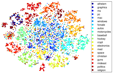
We listed the top 20 topic words of a 5-topic modeling problem as an example in Table I. From the table, we see that the topic words of the second and fifth topics produced by AnchorFree have an overlap of over 50%. Some informative topic words discovered by bDNMF, such as the words on anti-government activities or violence in the fifth topic, were not detected by AnchorFree. The above phenomena are observed in the other experiments too. We conjecture that the advanced experimental phenomena are caused by the fact that bDNMF not only avoids making additional assumptions but also benefits from the high clustering accuracy of the deep model. We show the latent representation of the documents in 20-newsgroups learned by MBN in Fig. 2. From the figure, we see that the latent representation has strong disriminability which may lead to high performance of DNMF.

Table II shows the comparison results on the 20-newsgroups corpus. From the table, we see that the DNMF variants achieve the highest clustering accuracy among the comparison methods. For example, the clustering accuracy of DNMF is more than $5\%$ absolutely higher than that of the runner-up method, i.e. LTM, when the number of the topics is 20 and between 4 and 15, and is at least $1\%$ higher than the latter in the other cases. Particularly, DNMF is significantly better than the NMF methods. The relative improvement of DNMF over NMF tends to be enlarged when the number of the topics increases, which demonstrates the effectiveness of the deep architecture of DNMF. In addition, the single-topic quality produced by sDNMF ranks the third in terms of coherence, which is inferior to AnchorFree and DFPA. The similarity count scores produced by sDNMF and cDNMF rank behind LTM and are higher than the other comparison methods, which indicates that DNMF is able to generate less overlapped topic words than the comparison methods except the probabilistic model—LTM.

TABLE III: Performance of the comparison algorithms on TDT2.

	#topics	PLSI	LDA	LapPLSI	LTM	SPA	SNPA	XRAY	AnchorFree	DFPA	bDNMF	sDNMF	cDNMF
ACC	3	0.5497	0.7932	0.9889	0.9872	0.7853	0.7854	0.7263	0.9738	0.8840	0.9954	0.9954	0.9954
	4	0.5187	0.7402	0.9831	0.9496	0.7291	0.7306	0.6782	0.9469	0.8151	0.9864	0.9864	0.9864
	5	0.4939	0.7013	0.9771	0.9443	0.6943	0.6986	0.6716	0.9186	0.8037	0.9808	0.9808	0.9808
	6	0.4678	0.6762	0.9683	0.9171	0.6452	0.6392	0.6267	0.9093	0.7888	0.9863	0.9863	0.9863
	7	0.4814	0.6570	0.9392	0.8649	0.6125	0.6105	0.6253	0.9024	0.7490	0.9566	0.9566	0.9566
	8	0.4721	0.6230	0.9457	0.8406	0.5818	0.5792	0.5736	0.8748	0.7233	0.9460	0.9460	0.9460
	9	0.4930	0.6481	0.9095	0.8092	0.5883	0.5832	0.5433	0.8690	0.7469	0.9575	0.9575	0.9575
	10	0.4883	0.6413	0.9017	0.7705	0.5642	0.5612	0.5319	0.8481	0.7305	0.9100	0.9100	0.9100
	15	0.5412	0.5941	0.8393	0.6861	0.4736	0.4694	0.4411	0.7963	0.6849	0.8613	0.8613	0.8613
	20	0.6290	0.6093	0.7606	0.6458	0.4593	0.4610	0.4358	0.7741	0.6776	0.8074	0.8074	0.8074
	25	0.6582	0.6095	0.7390	0.6325	0.4351	0.4367	0.4240	0.7392	0.6521	0.7664	0.7664	0.7664
rank		10.82	8.18	4.18	5.91	9.82	9.91	11.09	5.18	6.91	1.00	1.00	1.00
Coherence	3	-593.96	-427.39	-538.16	-678.43	-613.89	-613.89	-470.37	-419.13	-952.05	-336.00	-335.75	-341.63
	4	-573.30	-510.27	-562.86	-660.56	-592.47	-592.47	-447.67	-430.83	-888.18	-358.83	-350.48	-378.10
	5	-545.48	-509.78	-544.17	-634.29	-610.96	-610.96	-459.79	-406.99	-803.90	-377.58	-370.10	-381.37
	6	-536.32	-546.04	-554.52	-626.23	-642.78	-642.78	-466.89	-428.79	-831.70	-367.09	-364.30	-378.32
	7	-518.56	-543.56	-560.76	-597.02	-646.05	-646.05	-483.75	-397.79	-731.31	-396.75	-382.47	-401.49
	8	-519.33	-565.30	-555.45	-594.85	-657.72	-657.72	-477.15	-445.76	-704.81	-424.66	-399.95	-438.13
	9	-518.04	-570.69	-566.21	-594.83	-655.35	-655.35	-469.70	-418.12	-755.24	-415.77	-394.24	-439.97
	10	-518.91	-574.42	-573.86	-597.61	-668.08	-668.08	-508.05	-422.32	-715.69	-436.64	-414.76	-446.00
	15	-507.35	-617.88	-624.20	-579.34	-660.27	-660.27	-493.83	-433.01	-676.80	-519.91	-457.45	-523.13
	20	-557.22	-642.49	-660.17	-616.12	-679.49	-679.49	-497.80	-458.33	-627.00	-549.08	-478.88	-562.01
	25	-598.00	-666.08	-694.07	-635.02	-686.57	-686.57	-517.31	-469.48	-588.06	-572.57	-501.95	-589.15
rank		6.36	7.36	8.09	9.09	9.82	9.82	4.55	2.82	11.00	2.73	1.27	4.09
SimCount	3	216.60	2.78	419.04	24.44	16.10	16.10	22.44	4.08	50.08	0.42	0.38	0.72
	4	216.52	5.26	308.62	25.32	24.00	24.00	34.94	2.22	54.12	0.94	0.98	1.26
	5	209.04	8.02	282.56	24.74	29.36	29.36	57.68	4.94	112.22	1.26	1.08	1.48
	6	195.50	11.90	225.34	23.12	44.14	44.14	68.54	6.62	113.76	2.08	1.92	2.68
	7	176.74	16.06	204.44	25.40	53.52	53.52	95.46	4.48	191.38	3.16	2.98	3.00
	8	160.20	21.12	198.92	23.94	58.76	58.76	132.42	8.84	192.30	5.28	4.78	6.58
	9	161.46	25.46	163.18	24.34	74.48	74.48	159.44	9.92	285.06	6.98	6.32	8.06
	10	146.84	30.48	139.46	23.34	74.78	74.78	182.96	13.46	287.76	8.00	7.36	7.96
	15	91.82	65.08	80.14	23.26	189.44	189.44	481.58	40.78	690.20	25.66	23.40	22.90
	20	70.60	104.82	49.32	20.76	271.50	271.50	712.50	79.70	1056.20	50.22	44.90	43.64
	25	52.18	147.22	33.20	22.78	450.14	450.14	936.52	132.34	1741.28	72.52	66.32	57.28
rank		9.18	5.73	9.55	5.00	7.36	8.36	9.64	4.73	11.09	2.91	1.82	2.64

Table III shows the results on the TDT2 corpus. From the table, we see that the DNMF variants obtain the best performance in terms of clustering accuracy and similarity count, particularly when the number of topics is below 10. bDNMF and sDNMF outperform the comparison algorithms in terms of all three evaluation metrics, which demonstrates the advantage of the DNMF framework further. Although LapPLSI yields competitive clustering accuracy with DNMF, its performance in coherence and similarity count is significantly lower than DNMF. Although AnchorFree reaches a higher coherence rank than cDNMF, its similarity count scores are much higher than cDNMF.

TABLE IV: Performance of the comparison algorithms on Reuters-21578.

	#topics	PLSI	LDA	LapPLSI	LTM	SPA	SNPA	XRAY	AnchorFree	DFPA	bDNMF	sDNMF	cDNMF
ACC	3	0.6012	0.6269	0.7797	0.7445	0.7853	0.7854	0.7263	0.7904	0.7155	0.8591	0.8591	0.8591
	4	0.5253	0.5691	0.6966	0.6870	0.7291	0.7306	0.6782	0.7257	0.6587	0.7745	0.7745	0.7745
	5	0.4671	0.5290	0.6614	0.6198	0.6943	0.6986	0.6716	0.6480	0.6171	0.7160	0.7160	0.7160
	6	0.4648	0.5140	0.6165	0.5844	0.6452	0.6392	0.6267	0.6449	0.6169	0.6803	0.6803	0.6803
	7	0.4182	0.4628	0.6122	0.5820	0.6125	0.6105	0.6253	0.6472	0.5524	0.6948	0.6948	0.6948
	8	0.4049	0.4442	0.6067	0.5663	0.5818	0.5792	0.5736	0.6133	0.5504	0.6474	0.6474	0.6474
	9	0.3708	0.4064	0.5914	0.5490	0.5883	0.5832	0.5433	0.5886	0.5089	0.6244	0.6244	0.6244
	10	0.3765	0.4150	0.5628	0.5279	0.5642	0.5612	0.5319	0.5822	0.5386	0.6110	0.6110	0.6110
	15	0.3278	0.3545	0.4417	0.4210	0.4736	0.4694	0.4411	0.5198	0.5082	0.5189	0.5189	0.5189
	20	0.3371	0.3331	0.4083	0.3624	0.4593	0.4610	0.4358	0.5294	0.4585	0.4899	0.4899	0.4899
	25	0.3601	0.3373	0.3615	0.3553	0.4351	0.4367	0.4240	0.4684	0.4218	0.4702	0.4702	0.4702
rank		11.73	11.18	7.09	9.27	5.55	5.91	7.82	4.18	8.73	1.18	1.18	1.18
Coherence	3	-769.73	-674.14	-852.48	-943.56	-613.89	-613.89	-470.37	-827.28	-996.30	-760.47	-647.97	-759.97
	4	-786.89	-677.18	-813.51	-952.28	-592.47	-592.47	-447.67	-743.97	-1017.05	-719.27	-609.09	-726.13
	5	-785.65	-686.31	-838.40	-942.68	-610.96	-610.96	-459.79	-771.63	-1045.24	-752.04	-620.00	-746.92
	6	-805.24	-715.15	-854.96	-947.58	-642.78	-642.78	-466.89	-699.50	-1046.70	-764.52	-639.33	-766.60
	7	-806.03	-705.90	-804.15	-940.69	-646.05	-646.05	-483.75	-684.54	-982.35	-784.11	-654.06	-793.31
	8	-789.16	-762.92	-860.11	-967.17	-657.72	-657.72	-477.15	-722.67	-901.23	-825.28	-674.71	-826.15
	9	-793.27	-776.83	-841.44	-975.13	-655.35	-655.35	-469.70	-710.96	-858.33	-832.10	-699.29	-851.84
	10	-790.22	-776.46	-831.18	-945.31	-668.08	-668.08	-508.05	-703.61	-911.27	-808.08	-672.49	-828.59
	15	-837.89	-847.72	-848.49	-959.15	-660.27	-660.27	-493.83	-685.33	-950.77	-807.32	-669.67	-859.50
	20	-831.64	-903.37	-845.18	-955.92	-679.49	-679.49	-497.80	-678.43	-911.14	-846.06	-709.83	-916.70
	25	-827.83	-902.68	-831.65	-932.96	-686.57	-686.57	-517.31	-667.75	-905.43	-851.30	-708.87	-969.11
rank		7.73	6.45	9.18	11.45	2.27	3.27	1.00	5.36	11.27	7.27	4.00	8.73
SimCount	3	3.20	230.84	765.22	45.12	16.10	16.10	22.44	7.26	49.70	3.60	3.10	2.96
	4	6.46	218.28	759.62	39.60	24.00	24.00	34.94	12.00	51.22	7.84	5.98	6.56
	5	9.32	223.40	694.86	38.76	29.36	29.36	57.68	16.90	104.92	11.16	9.28	9.60
	6	12.48	228.04	661.24	40.58	44.14	44.14	68.54	19.62	109.74	16.36	13.74	13.62
	7	21.22	221.34	721.32	41.66	53.52	53.52	95.46	33.40	190.46	22.00	17.68	18.08
	8	24.60	277.82	653.54	46.96	58.76	58.76	132.42	61.60	189.82	34.20	28.68	27.92
	9	33.56	332.46	628.38	55.42	74.48	74.48	159.44	69.76	289.18	43.80	35.90	33.80
	10	39.68	276.18	607.02	51.18	74.78	74.78	182.96	86.00	287.54	48.60	41.02	38.22
	15	76.02	209.54	658.12	46.20	189.44	189.44	481.58	126.70	658.42	137.28	121.78	90.40
	20	130.54	222.64	637.50	49.44	271.50	271.50	712.50	226.02	1000.46	227.28	198.32	137.78
	25	194.98	202.88	615.52	48.94	450.14	450.14	936.52	339.68	1607.34	296.32	251.80	148.94
rank		2.00	9.55	11.55	5.09	6.73	6.73	9.27	5.91	10.64	4.64	2.73	2.18

Table IV shows the performance of the comparison methods on the Reuters-21578 corpus. From the table, we see that the DNMF variants reach the highest clustering accuracy. Although it seems that they do not reach the top performance in terms of coherence and similarity count soly, they balance the coherence and similarity count which evaluate two contradict aspects of a topic model. For example, although the coherence of sDNMF ranks behind XRAY and SPA, its similarity count is much higher than the latter. Although the similarity count of sDNMF ranks behind PLSI, its coherence is higher than PLSI as well. If we average the coherence and similarity count ranking lists, it is clear that sDNMF performs the best.

TABLE V: Average ranks of the comparison methods on all three data sets. The “Coh.+SimCount” ranking list is the average of the lists in coherence and similarity count. The “overall” ranking list is the average of the lists in the three evaluation metrics.

	PLSI	LDA	LapPLSI	LTM	SPA	SNPA	XRAY	AnchorFree	DFPA	bDNMF	sDNMF	cDNMF
ACC	10.58	8.75	6.42	6.43	8.62	8.71	10.30	5.05	6.95	1.06	1.06	1.06
Coherence	8.33	6.27	8.76	9.65	5.60	5.60	5.85	3.19	8.02	5.27	3.12	7.34
SimCount	7.36	7.76	10.70	3.76	6.06	6.06	8.37	6.75	10.64	4.42	2.52	2.61
Coh.+SimCount	7.85	7.02	9.73	6.71	5.83	5.83	7.11	4.97	9.33	4.85	2.82	4.98
Overall	8.76	7.59	8.63	6.61	6.76	6.79	8.17	5.00	8.54	3.58	2.23	3.67

We summarize the ranking lists of the comparison methods on the three corpora in Table V. From the overall ranking list in the table, we see that (i) the DNMF variants perform the best generally, followed by AnchorFree and LTM, and (ii) sDNMF performs the best among the three DNMF variants. If we take a look at the average ranking list over coherence and similarity count, we find that sDNMF reach the top performance, while bDNMF and sDNMF behave similarly with AnchorFree—a recent advanced NMF method that avoids the anchor-word assumption.

(a)

(b)

Figure 3: Performance of cDNMF with respect to hyperparameter $\lambda_{1}$ in terms of coherence and similarity count.

(a)

(b)

Figure 4: Performance of cDNMF with respect to hyperparameter $\lambda_{2}$.

(a)

(b)

Figure 5: Clustering accuracy of DNMF with respect to hyperparameters $\delta$ and $M$.

(a)

(b)

Figure 6: Performance of the DNMF variants with respect to hyperparameter $\delta$ on 20-newsgroups in terms of coherence and similarity count.

(a)

(b)

Figure 7: Performance of the DNMF variants with respect to hyperparameter $\delta$ on TDT2 in terms of coherence and similarity count.

(a)

(b)

Figure 8: Performance of the DNMF variants with respect to hyperparameter $\delta$ on Reuters-21578 in terms of coherence and similarity count.

(a)

(b)

Figure 9: Performance of the DNMF variants with respect to hyperparameter $M$ on 20-newsgroups in terms of coherence and similarity count.

(a)

(b)

Figure 10: Performance of the DNMF variants with respect to hyperparameter $M$ on TDT2 in terms of coherence and similarity count.

(a)

(b)

Figure 11: Performance of the DNMF variants with respect to hyperparameter $V$ on Reuters-21578 in terms of coherence and similarity count.

3.5 Effects of the hyperparameters of DNMF

To study how the hyperparameters of DNMF affect the performance, we searched the hyperparameters in grid. To prevent exhaust search, when we studied a hyperparameter, we fixed the other hyperparameters to their default values.

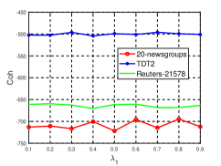
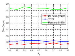
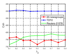
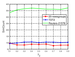
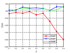
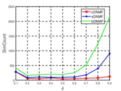
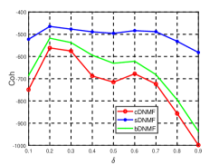
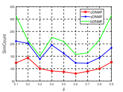
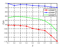
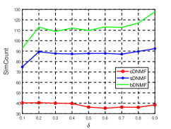
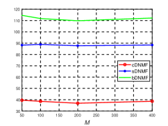
We first studied the two regularization hyperparameters of cDNMF $\lambda_{1}$ and $\lambda_{2}$ in terms of coherence and similarity count by searching the two hyperparametres in grid from 0.1 to 0.9. The results are shown in Figs. 3 and 4. From the figures, we see that cDNMF is in sensitive to the two hyperparameters.

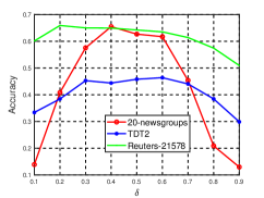
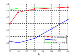
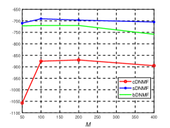
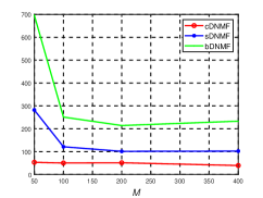
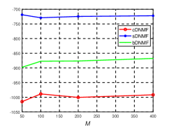
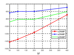
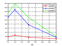
Then, we studied the hyperparameters $\delta$ and $M$ of the deep model in DNMF in terms of all three evaluation metrics, in which $\delta$ is searched from 0.1 to 0.9 and $M$ searched from 10 to 400. Figure 5 shows the clustering accuracy of DNMF with respect to the two hyperparameters. Figures 6 to 8 shows the coherence and similarity count of the DNMF variants with respect to $\delta$ on the three corpora respectively. Figures 9 to 11 shows the coherence and similarity count of the DNMF variants with respect to $M$ on the three corpora respectively. From the figures, we see that although the DNMF variants are sensitive to $\delta$ and $M$, we can clearly find the regulations. For the hyperparameter $\delta$, we observe from Fig. 5a and Figs. 6 to 8 that, when $\delta$ is set around the default value $0.5$, all DNMF variants approach to the top performance in all cases.

For the hyperparameter $M$, we see from Fig. 5b that enlarging $M$ clearly improves the clustering accuracy of all DNMF variants. From Figs. 9a, 10a, and 11a, we see that the performance of all DNNF variants is improved generally along with the increase of $M$ in terms of coherence in all cases except that the performance of bDNMF and sDNMF is getting worse on 20-newsgroups. From Figs. 9b, 10b, and 11b, we see that the similarity count scores of all DNMF variants are getting smaller generally along with the increase of $M$ on 20-newsgroups and TDT2. It is interesting to observe that the similarity count scores of the DNMF variants first get larger and then smaller along with the increase of $M$ on Reuters-21578, with a peak at $M=100$. Nonetheless, the DNMF variants approach to the lowest similarity count scores at $M=400$ in all cases. We can imagine that, when we set $M$ larger than 400, the performance may be further improved with the expense of higher computational complexity. To balance the performance and the computational complexity, it is reasonable to set $M=400$.

4 Conclusions

In this paper, we have proposed a deep NMF topic modeling framework and evaluated its effectiveness with three implementations. To our knowledge, this is the first deep NMF topic modeling framework. The novelty of DNMF lies in the following aspects. First, we proposed a novel unsupervised deep NMF framework that is fundamentally different from existing deep learning based topic modeling methods. It takes the unsupervised deep learning as a constraint of NMF. It is a general framework that can incorporate many types of deep models and NMF methods. To evaluate its effectiveness, we implemented three DNMF algorithms, denoted as bDNMF, sDNMF, and cDNMF. bDNMF takes the sparse output of the deep model as the topic-document matrix directly, which formulates bDNMF as a supervised regression problem with a nonnegative constraint on the word-topic matrix. sDNMF takes the output of the deep model as a mask of the topic-document matrix, and solves the NMF problem by the alternative iterative optimization, which relaxes the strong constraint on the topic-document matrix in bDNMF. cDNMF takes the output of the deep model as a regularization, which further relaxes the constraint on the topic-document matrix. To our knowledge, the regularization terms in cDNMF is novel. Finally, we applied multilayer bootstrap networks for document clustering. It reaches the state-of-the-art performance given the high-dimensional sparse TF-IDF statistics of the documents, which further boosts the overall performance of the DNMF implementations. We have conducted an extensive experimental comparison with 9 representative comparison methods covering probabilistic topic models, NMF topic models, and deep topic modeling on three benchmark datasets—20-newsgroups, TDT2, and Reuters-21578. Experimental results show that the proposed DNMF variants outperform the comparison methods significantly in terms of clustering accuracy, coherence, and similarity count. Moreover, although the DNMF variants are relative sensitive to the hyperparameter $\delta$, we always find a robust working range across the corpora, which demonstrates the robustness of the DNMF variants in real-world applications.

Appendix A

Before we prove Theorem 1, we first give the definition of an upper bound auxiliary function.

Definition 1.

$\mathcal{G}(u,u^{\prime})$ is an upper bound auxiliary function for $g(u)$ if the following conditions are satisfied:

$$\begin{split}\mathcal{G}(u,u^{\prime})\geq g(u),\mathcal{G}(u,u)=g(u)\end{split}$$ (52)

Corollary 1.

If $\mathcal{G}(\cdot,\cdot)$ is an upper bound auxiliary function for $g(u)$, then $g(u)$ is non-increasing under the update rule

$$\begin{split}u^{t+1}=\arg\min_{u}\mathcal{G}(u,u^{t})\end{split}$$ (53)

Proposition 1.

For any matrices $\mathbf{A}\in\mathbb{R}^{n\times n}_{+}$, $\mathbf{B}\in\mathbb{R}^{k\times k}_{+}$, $\mathbf{E}\in\mathbb{R}^{n\times k}_{+}$, $\mathbf{E}^{\prime}\in\mathbb{R}^{n\times k}_{+}$, with $\mathbf{A}$ and $\mathbf{B}$ being symmetric matrices, the following inequality holds [61]:

$$\begin{split}\sum_{i=1}^{n}\sum_{j=1}^{k}\frac{[\mathbf{A}\mathbf{E}^{\prime}\mathbf{B}]_{ij}[\mathbf{E}]_{ij}^{2}}{[\mathbf{E}]^{\prime}_{ij}}\geq\mbox{Tr}(\mathbf{E}^{T}\mathbf{A}\mathbf{E}\mathbf{B})\end{split}$$ (54)

Definition 2.

A function can be represented as an infinite sum of terms that are calculated from the values of the function’s derivatives at a single point, which can be formulated as follows:

$$\begin{split}f(x)=\sum_{n=0}^{\infty}\frac{f^{(n)}(a)}{n!}(y-a)^{n}\end{split}$$ (55)

Given the above definitions, the objective function of cDNMF (29) with respect to the three univariate functions are obtained as follows:

$$\begin{split}\mathcal{O}_{\mathbf{C}}=\|\mathbf{D}-\mathbf{C}{\mathbf{W}}\|_{F}^{2}+\lambda_{1}\|\mathbf{C}\mathbf{C}^{T}-\mathbf{D}\mathbf{D}^{T}\|_{F}^{2}\end{split}$$ (56)

$$\begin{split}\mathcal{O}_{\mathbf{W}}=\|\mathbf{D}-\mathbf{C}{\mathbf{W}}\|_{F}^{2}+\lambda_{2}\|f(\mathbf{D})-\mathbf{T}{\mathbf{W}}\|_{F}^{2}\end{split}$$ (57)

$$\begin{split}\mathcal{O}_{\mathbf{T}}=\lambda_{2}\|f(\mathbf{D})-\mathbf{T}{\mathbf{W}}\|_{F}^{2}\end{split}$$ (58)

Then, we have the following three lemmas.

Lemma 1.

The auxiliary function for $\mathcal{O}(\mathbf{C})$ is as follows:

$$\begin{split}&\mathcal{G}([\mathbf{C}]_{ij},[\mathbf{C}^{\prime}]_{ij})=\mathcal{O}_{\mathbf{C}}+[-2\mathbf{D}\mathbf{W}^{T}+2\mathbf{C}{\mathbf{W}}{\mathbf{W}}^{T}\\ &-4\lambda_{1}\mathbf{D}\mathbf{D}^{T}\mathbf{C}+4\lambda_{1}\mathbf{C}\mathbf{C}^{T}\mathbf{C}]_{ij}([\mathbf{C}]_{ij}-[\mathbf{C}^{\prime}]_{ij})\\ &+\frac{1}{3!}4\lambda_{1}[\mathbf{C}]_{ij}([\mathbf{C}]_{ij}-[\mathbf{C}^{\prime}]_{ij})^{3}+\frac{1}{4!}4\lambda_{1}([\mathbf{C}]_{ij}-[\mathbf{C}^{\prime}]_{ij})^{4}\\ &+\frac{1}{2}\frac{2[\mathbf{C}{\mathbf{W}}{\mathbf{W}}^{T}]_{ij}+4\lambda_{1}[\mathbf{C}\mathbf{C}^{T}\mathbf{C}]_{ij}}{[\mathbf{C}]_{ij}}([\mathbf{C}]_{ij}-[\mathbf{C}^{\prime}]_{ij})^{2}\end{split}$$ (59)

Proof.

It is obvious that $\mathcal{G}(\mathbf{C},\mathbf{C})=\mathcal{O}_{\mathbf{C}}(\mathbf{C})$, we only need to prove that $\mathcal{G}(\mathbf{C},\mathbf{C}^{\prime})\geq\mathcal{O}_{\mathbf{C}}(\mathbf{C})$. The first-order partial derivative of (56) in element-wise is

$$\begin{split}&\frac{\partial\mathcal{O}_{\mathbf{C}}}{\partial[\mathbf{C}]_{ij}}\\ =&[-2\mathbf{D}\mathbf{W}^{T}+2\mathbf{C}{\mathbf{W}}{\mathbf{W}}^{T}-4\lambda_{1}\mathbf{D}\mathbf{D}^{T}\mathbf{C}+4\lambda_{1}\mathbf{C}\mathbf{C}^{T}\mathbf{C}]_{ij}\end{split}$$ (60)

The second-order derivative of (56) with respect to $\mathbf{C}$ is

$$\begin{split}\frac{\partial^{2}\mathcal{O}_{\mathbf{C}}}{\partial[\mathbf{C}]_{ij}\partial[\mathbf{C}]_{ij}}=[2{\mathbf{W}}{\mathbf{W}}^{T}]_{jj}-4\lambda_{1}[\mathbf{D}\mathbf{D}^{T}]_{ii}+4\lambda_{1}[\mathbf{C}\mathbf{C}^{T}]_{ii}\end{split}$$ (61)

The third-order partial derivative of (56) is

$$\begin{split}\frac{\partial^{3}\mathcal{O}_{\mathbf{C}}}{\partial[\mathbf{C}]_{ij}\partial[\mathbf{C}]_{ij}\partial[\mathbf{C}]_{ij}}=4\lambda_{1}[\mathbf{C}]_{ij}\end{split}$$ (62)

The fourth-order partial derivative of (56) is

$$\begin{split}\frac{\partial^{4}\mathcal{O}_{\mathbf{C}}}{\partial[\mathbf{C}]_{ij}\partial[\mathbf{C}]_{ij}\partial[\mathbf{C}]_{ij}\partial[\mathbf{C}]_{ij}}=4\lambda_{1}\end{split}$$ (63)

According to the Taylor expansion in Definition (55), we can rewrite (56) to its Taylor expansion form:

$$\begin{split}\mathcal{O}_{\mathbf{C}}(c_{ij})=&\mathcal{O}_{\mathbf{C}}+\frac{\partial\mathcal{O}_{\mathbf{C}}}{\partial c_{ij}}(c_{ij}-[\mathbf{C}]_{ij})\\ &+\frac{1}{2}\frac{\partial^{2}\mathcal{O}_{\mathbf{C}}}{\partial c_{ij}\partial c_{ij}}(c_{ij}-[\mathbf{C}]_{ij})^{2}\\ &+\frac{1}{3!}\frac{\partial^{3}\mathcal{O}_{\mathbf{C}}}{\partial c_{ij}\partial c_{ij}\partial c_{ij}}(c_{ij}-[\mathbf{C}]_{ij})^{3}\\ &+\frac{1}{4!}\frac{\partial^{4}\mathcal{O}_{\mathbf{C}}}{\partial c_{ij}\partial c_{ij}\partial c_{ij}\partial c_{ij}}(c_{ij}-[\mathbf{C}]_{ij})^{4}\end{split}$$ (64)

The upper bound auxiliary function for (56) is defined as

$$\begin{split}&\mathcal{G}([\mathbf{C}]_{ij},[\mathbf{C}^{\prime}]_{ij})=\mathcal{O}_{\mathbf{C}}+\frac{\partial\mathcal{O}_{\mathbf{C}}}{\partial[\mathbf{C}]_{ij}}([\mathbf{C}]_{ij}-[\mathbf{C}^{\prime}]_{ij})\\ &+\frac{1}{3!}\frac{\partial^{3}\mathcal{O}_{\mathbf{C}}}{\partial[\mathbf{C}]_{ij}\partial[\mathbf{C}]_{ij}\partial[\mathbf{C}]_{ij}}([\mathbf{C}]_{ij}-[\mathbf{C}^{\prime}]_{ij})^{3}\\ &+\frac{1}{4!}\frac{\partial^{4}\mathcal{O}_{\mathbf{C}}}{\partial[\mathbf{C}]_{ij}\partial[\mathbf{C}]_{ij}\partial[\mathbf{C}]_{ij}\partial[\mathbf{C}]_{ij}}([\mathbf{C}]_{ij}-[\mathbf{C}^{\prime}]_{ij})^{4}\\ &+\frac{1}{2}\frac{2[\mathbf{C}{\mathbf{W}}{\mathbf{W}}^{T}]_{ij}+4\lambda_{1}[\mathbf{C}\mathbf{C}^{T}\mathbf{C}]_{ij}}{[\mathbf{C}]_{ij}}([\mathbf{C}]_{ij}-[\mathbf{C}^{\prime}]_{ij})^{2}\end{split}$$ (65)

Substituting (64) into (65), we find that $\mathcal{G}(\mathbf{C},\mathbf{C}^{\prime})\geq\mathcal{O}_{\mathbf{C}}(\mathbf{C})$ is equivalent to

$$\begin{split}&\frac{1}{2}\frac{2[\mathbf{C}{\mathbf{W}}{\mathbf{W}}^{T}]_{ij}+4\lambda_{1}[\mathbf{C}\mathbf{C}^{T}\mathbf{C}]_{ij}}{[\mathbf{C}]_{ij}}([\mathbf{C}]_{ij}-[\mathbf{C}^{\prime}]_{ij})^{2}\\ &\geq\frac{1}{2}\left([2{\mathbf{W}}{\mathbf{W}}^{T}]_{jj}-4\lambda_{1}[\mathbf{D}\mathbf{D}^{T}]_{ii}+4\lambda_{1}[\mathbf{C}\mathbf{C}^{T}]_{ii}\right)([\mathbf{C}]_{ij}-[\mathbf{C}^{\prime}]_{ij})^{2}\end{split}$$ (66)

Because we have

$$\begin{split}&\frac{[\mathbf{C}{\mathbf{W}}{\mathbf{W}}^{T}]_{ij}}{[\mathbf{C}]_{ij}}=\frac{\sum_{j}\left([\mathbf{C}]_{ij}\times[{\mathbf{W}}{\mathbf{W}}^{T}]_{jj}\right)}{[\mathbf{C}]_{ij}}\\ &\geq\frac{[\mathbf{C}]_{ij}\times[{\mathbf{W}}{\mathbf{W}}^{T}]_{jj}}{[\mathbf{C}]_{ij}}=[{\mathbf{W}}{\mathbf{W}}^{T}]_{jj}\end{split}$$ (67)

$$\begin{split}&\frac{[\mathbf{C}\mathbf{C}^{T}\mathbf{C}]_{ij}}{[\mathbf{C}]_{ij}}=\frac{\sum_{j}\left([\mathbf{C}\mathbf{C}^{T}]_{jj}\times[\mathbf{C}]_{ij}\right)}{[\mathbf{C}]_{ij}}\\ &\geq\frac{[\mathbf{C}\mathbf{C}^{T}]_{ii}\times[\mathbf{C}]_{ij}}{[\mathbf{C}]_{ij}}=[\mathbf{C}\mathbf{C}^{T}]_{ii}\end{split}$$ (68)

we can conclude that (66) holds, and (65) is an upper bound auxiliary function for (56). Because the elements of matrix $\mathbf{C}$ is nonnegative, the third and fourth order partial derivatives are larger than zero and (65) is a convex function, its minimum value can be achieved at

$$\begin{split}&[\mathbf{C}^{\prime}]_{ij}\\ &=[\mathbf{C}]_{ij}-\frac{[-2\mathbf{D}\mathbf{W}^{T}+2\mathbf{C}{\mathbf{W}}{\mathbf{W}}^{T}-4\lambda_{1}\mathbf{D}\mathbf{D}^{T}\mathbf{C}+4\lambda_{1}\mathbf{C}\mathbf{C}^{T}\mathbf{C}]_{ij}}{2\times\frac{1}{2}\frac{[2\mathbf{C}{\mathbf{W}}{\mathbf{W}}^{T}]_{ij}+4\lambda_{1}[\mathbf{C}\mathbf{C}^{T}\mathbf{C}]_{ij}}{[\mathbf{C}]_{ij}}([\mathbf{C}]_{ij}-[\mathbf{C}^{\prime}]_{ij})^{2}}\\ &=[\mathbf{C}]_{ij}\frac{[\mathbf{D}\mathbf{W}^{T}]_{ij}+2\lambda_{1}[\mathbf{D}\mathbf{D}^{T}\mathbf{C}]_{ij}}{[\mathbf{C}{\mathbf{W}}{\mathbf{W}}^{T}]_{ij}+2\lambda_{1}[\mathbf{C}\mathbf{C}^{T}\mathbf{C}]_{ij}}\end{split}$$ (69)

Lemma 1 is proved. ∎

Lemma 2.

Given Proposition 1, the auxiliary function for $\mathcal{O}(\mathbf{W})$ is as follows:

$$\begin{split}\mathcal{G}(\mathbf{W},\mathbf{W}^{\prime})&=-2\lambda_{2}\mbox{Tr}(f(\mathbf{D}){\mathbf{W}}^{T}\mathbf{T}^{T})-2\mbox{Tr}(\mathbf{D}\mathbf{W}^{T}\mathbf{C}^{T})\\ &+\sum_{ij}\frac{[\mathbf{C}^{T}\mathbf{C}{\mathbf{W}}]_{ij}{[{\mathbf{W}}^{\prime}]}^{2}_{ij}}{[{\mathbf{W}}]_{ij}}+\lambda_{2}\sum_{ij}\frac{[\mathbf{T}^{T}\mathbf{T}{\mathbf{W}}]_{ij}{[{\mathbf{W}}^{\prime}]}^{2}_{ij}}{[{\mathbf{W}}]_{ij}}\end{split}$$ (70)

Lemma 3.

The auxiliary function for $\mathcal{O}(\mathbf{T})$ is as follows:

$$\begin{split}\mathcal{G}(\mathbf{T},\mathbf{T}^{\prime})=-2\lambda_{2}\mbox{Tr}(f(\mathbf{D}){\mathbf{W}}^{T}\mathbf{T}^{T})+\lambda_{2}\sum_{ij}\frac{[\mathbf{T}{\mathbf{W}}{\mathbf{W}}^{T}]_{ij}{[\mathbf{T}^{\prime}]}^{2}_{ij}}{[\mathbf{T}]_{ij}}\end{split}$$ (71)

With the above lemmas, we derive the update rules for each variable by minimizing their corresponding auxiliary functions:

$$\begin{split}&\frac{\partial\mathcal{G}(\mathbf{C},\mathbf{C}^{\prime})}{\partial[\mathbf{C}^{\prime}]_{ij}}=-2[\mathbf{D}\mathbf{W}^{T}]_{ij}+2\frac{[\mathbf{C}\mathbf{W}\mathbf{W}^{T}]_{ij}[\mathbf{C}^{\prime}]_{ij}}{[\mathbf{C}]_{ij}}\\ &-4\lambda_{1}[\mathbf{D}\mathbf{D}^{T}\mathbf{C}]_{ij}+4\lambda_{1}\frac{[\mathbf{C}\mathbf{C}^{T}\mathbf{C}]_{ij}{[\mathbf{C}^{\prime}]}_{ij}}{[\mathbf{C}]_{ij}}=0\end{split}$$ (72)

$$\begin{split}&\frac{\partial\mathcal{G}(\mathbf{W},\mathbf{W}^{\prime})}{\partial[\mathbf{W}^{\prime}]_{ij}}=-2\lambda_{2}[\mathbf{T}^{T}f(\mathbf{D})]_{ij}-2[\mathbf{C}^{T}\mathbf{D}]_{ij}\\ &+2\frac{[\mathbf{C}^{T}\mathbf{C}{\mathbf{W}}]_{ij}{[\mathbf{W}^{\prime}]}_{ij}}{[\mathbf{W}]_{ij}}+2\lambda_{2}\frac{[\mathbf{T}^{T}\mathbf{T}{\mathbf{W}}]_{ij}{[\mathbf{W}^{\prime}]}_{ij}}{[\mathbf{W}]_{ij}}=0\end{split}$$ (73)

$$\begin{split}&\frac{\partial\mathcal{G}(\mathbf{T},\mathbf{T}^{\prime})}{\partial[\mathbf{T}^{\prime}]_{ij}}=-2[f(\mathbf{D}){\mathbf{W}}^{T}]_{ij}+2\frac{[\mathbf{T}{\mathbf{W}}{\mathbf{W}}^{T}]_{ij}{[\mathbf{T}^{\prime}]}_{ij}}{[\mathbf{T}]_{ij}}=0\end{split}$$ (74)

which derives

$$\begin{split}[\mathbf{C}^{\prime}]_{ij}=[\mathbf{C}]_{ij}\frac{[\mathbf{D}\mathbf{W}^{T}]_{ij}+2\lambda_{1}[\mathbf{D}\mathbf{D}^{T}\mathbf{C}]_{ij}}{[\mathbf{C}{\mathbf{W}}{\mathbf{W}}^{T}]_{ij}+2\lambda_{1}[\mathbf{C}\mathbf{C}^{T}\mathbf{C}]_{ij}}\end{split}$$ (75)

$$\begin{split}[\mathbf{W}^{\prime}]_{ij}=[\mathbf{W}]_{ij}\frac{\lambda_{2}[\mathbf{T}^{T}f(\mathbf{D})]_{ij}+[\mathbf{C}^{T}\mathbf{D}]_{ij}}{[\mathbf{C}^{T}\mathbf{C}\mathbf{W}]_{ij}+\lambda_{2}[\mathbf{T}^{T}\mathbf{T}{\mathbf{W}}]_{ij}}\end{split}$$ (76)

$$\begin{split}[\mathbf{T}^{\prime}]_{ij}=[\mathbf{T}]_{ij}\frac{[f(\mathbf{D}){\mathbf{W}}^{T}]_{ij}}{[\mathbf{T}{\mathbf{W}}{\mathbf{W}}^{T}]_{ij}}\end{split}$$ (77)

It can be proved that the three update rules (44), (43) and (45) are equivalent to (75), (76) and (77), respectively. Because the objective function in (29) is lower bounded by 0, the modified DNMF converges to a stationary point. Theorem 1 is proved.

References

- [1] David M Blei, Andrew Y Ng, and Michael I Jordan, “Latent dirichlet allocation,” Journal of machine Learning research, vol. 3, no. Jan, pp. 993–1022, 2003.
- [2] Jaegul Choo, Changhyun Lee, Chandan K Reddy, and Haesun Park, “Utopian: User-driven topic modeling based on interactive nonnegative matrix factorization,” IEEE transactions on visualization and computer graphics, vol. 19, no. 12, pp. 1992–2001, 2013.
- [3] Nicolas Gillis and Stephen A Vavasis, “Fast and robust recursive algorithmsfor separable nonnegative matrix factorization,” IEEE transactions on pattern analysis and machine intelligence, vol. 36, no. 4, pp. 698–714, 2013.
- [4] Abhishek Kumar, Vikas Sindhwani, and Prabhanjan Kambadur, “Fast conical hull algorithms for near-separable non-negative matrix factorization,” in International Conference on Machine Learning, 2013, pp. 231–239.
- [5] Nicolas Gillis, “Successive nonnegative projection algorithm for robust nonnegative blind source separation,” SIAM Journal on Imaging Sciences, vol. 7, no. 2, pp. 1420–1450, 2014.
- [6] Xiao Fu, Wing-Kin Ma, Tsung-Han Chan, and José M Bioucas-Dias, “Self-dictionary sparse regression for hyperspectral unmixing: Greedy pursuit and pure pixel search are related,” IEEE Journal of Selected Topics in Signal Processing, vol. 9, no. 6, pp. 1128–1141, 2015.
- [7] Y. Chen, J. Wu, J. Lin, R. Liu, H. Zhang, and Z. Ye, “Affinity regularized non-negative matrix factorization for lifelong topic modeling,” IEEE Transactions on Knowledge and Data Engineering, pp. 1–1, 2019.
- [8] Xuelong Li, Guosheng Cui, and Yongsheng Dong, “Graph regularized non-negative low-rank matrix factorization for image clustering,” IEEE transactions on cybernetics, vol. 47, no. 11, pp. 3840–3853, 2016.
- [9] Thomas L. Griffiths, Michael I. Jordan, Joshua B. Tenenbaum, and David M. Blei, “Hierarchical topic models and the nested chinese restaurant process,” in Advances in Neural Information Processing Systems 16, S. Thrun, L. K. Saul, and B. Schölkopf, Eds., pp. 17–24. MIT Press, 2004.
- [10] Jen-Tzung Chien, “Hierarchical theme and topic modeling,” IEEE transactions on neural networks and learning systems, vol. 27, no. 3, pp. 565–578, 2015.
- [11] Daniel Ramage, Christopher D Manning, and Susan Dumais, “Partially labeled topic models for interpretable text mining,” in Proceedings of the 17th ACM SIGKDD international conference on Knowledge discovery and data mining, 2011, pp. 457–465.
- [12] Finale Doshi-Velez and Been Kim, “Towards a rigorous science of interpretable machine learning,” arXiv preprint arXiv:1702.08608, 2017.
- [13] Y. Zheng, Y. Zhang, and H. Larochelle, “A deep and autoregressive approach for topic modeling of multimodal data,” IEEE Transactions on Pattern Analysis and Machine Intelligence, vol. 38, no. 6, pp. 1056–1069, 2016.
- [14] J. Chien and C. Lee, “Deep unfolding for topic models,” IEEE Transactions on Pattern Analysis and Machine Intelligence, vol. 40, no. 2, pp. 318–331, 2018.
- [15] George Trigeorgis, Konstantinos Bousmalis, Stefanos Zafeiriou, and Björn W Schuller, “A deep matrix factorization method for learning attribute representations,” IEEE transactions on pattern analysis and machine intelligence, vol. 39, no. 3, pp. 417–429, 2016.
- [16] Linlin Zong, Xianchao Zhang, Long Zhao, Hong Yu, and Qianli Zhao, “Multi-view clustering via multi-manifold regularized non-negative matrix factorization,” Neural Networks, vol. 88, pp. 74 – 89, 2017.
- [17] Pengtao Xie and Eric P. Xing, “Integrating document clustering and topic modeling,” in Proceedings of the Twenty-Ninth Conference on Uncertainty in Artificial Intelligence, Arlington, Virginia, USA, 2013, UAI 13, p. 694 C703, AUAI Press.
- [18] Yu-Xiong Wang and Yu-Jin Zhang, “Nonnegative matrix factorization: A comprehensive review,” IEEE Transactions on Knowledge and Data Engineering, vol. 25, no. 6, pp. 1336–1353, 2012.
- [19] Junyuan Xie, Ross Girshick, and Ali Farhadi, “Unsupervised deep embedding for clustering analysis,” in International conference on machine learning, 2016, pp. 478–487.
- [20] Christos H Papadimitriou, Prabhakar Raghavan, Hisao Tamaki, and Santosh Vempala, “Latent semantic indexing: A probabilistic analysis,” Journal of Computer and System Sciences, vol. 61, no. 2, pp. 217–235, 2000.
- [21] Deng Cai, Qiaozhu Mei, Jiawei Han, and Chengxiang Zhai, “Modeling hidden topics on document manifold,” in Proceedings of the 17th ACM conference on Information and knowledge management. ACM, 2008, pp. 911–920.
- [22] Deng Cai, Xuanhui Wang, and Xiaofei He, “Probabilistic dyadic data analysis with local and global consistency,” in Proceedings of the 26th annual international conference on machine learning. ACM, 2009, pp. 105–112.
- [23] Xiao Fu, Kejun Huang, Nicholas D Sidiropoulos, Qingjiang Shi, and Mingyi Hong, “Anchor-free correlated topic modeling,” IEEE transactions on pattern analysis and machine intelligence, vol. 41, no. 5, pp. 1056–1071, 2018.
- [24] Ricardo Henao, Zhe Gan, James Lu, and Lawrence Carin, “Deep poisson factor modeling,” in Advances in Neural Information Processing Systems, 2015, pp. 2800–2808.
- [25] Yee W Teh, Michael I Jordan, Matthew J Beal, and David M Blei, “Sharing clusters among related groups: Hierarchical dirichlet processes,” in Advances in neural information processing systems, 2005, pp. 1385–1392.
- [26] Weifeng Li, Junming Yin, and Hsinchsun Chen, “Supervised topic modeling using hierarchical dirichlet process-based inverse regression: Experiments on e-commerce applications,” IEEE Transactions on Knowledge and Data Engineering, vol. 30, no. 6, pp. 1192–1205, 2017.
- [27] John Paisley, Chong Wang, David M Blei, and Michael I Jordan, “Nested hierarchical dirichlet processes,” IEEE Transactions on Pattern Analysis and Machine Intelligence, vol. 37, no. 2, pp. 256–270, 2014.
- [28] David M Blei, Thomas L Griffiths, and Michael I Jordan, “The nested chinese restaurant process and bayesian nonparametric inference of topic hierarchies,” Journal of the ACM (JACM), vol. 57, no. 2, pp. 7, 2010.
- [29] Sanjeev Arora, Rong Ge, and Ankur Moitra, “Learning topic models–going beyond svd,” in 2012 IEEE 53rd Annual Symposium on Foundations of Computer Science. IEEE, 2012, pp. 1–10.
- [30] Jen-Tzung Chien and Chao-Hsi Lee, “Deep unfolding for topic models,” IEEE transactions on pattern analysis and machine intelligence, vol. 40, no. 2, pp. 318–331, 2017.
- [31] Geoffrey E Hinton and Ruslan R Salakhutdinov, “Replicated softmax: an undirected topic model,” in Advances in neural information processing systems, 2009, pp. 1607–1614.
- [32] Martin Gerlach, Tiago P Peixoto, and Eduardo G Altmann, “A network approach to topic models,” Science advances, vol. 4, no. 7, pp. eaaq1360, 2018.
- [33] Mikhail Yurochkin and XuanLong Nguyen, “Geometric dirichlet means algorithm for topic inference,” in Advances in Neural Information Processing Systems, 2016, pp. 2505–2513.
- [34] Hugo Larochelle and Stanislas Lauly, “A neural autoregressive topic model,” in Advances in Neural Information Processing Systems, 2012, pp. 2708–2716.
- [35] Yin Zheng, Yu-Jin Zhang, and Hugo Larochelle, “A deep and autoregressive approach for topic modeling of multimodal data,” IEEE transactions on pattern analysis and machine intelligence, vol. 38, no. 6, pp. 1056–1069, 2015.
- [36] Zhe Gan, Changyou Chen, Ricardo Henao, David Carlson, and Lawrence Carin, “Scalable deep poisson factor analysis for topic modeling,” in International Conference on Machine Learning, 2015, pp. 1823–1832.
- [37] Rajesh Ranganath, Linpeng Tang, Laurent Charlin, and David Blei, “Deep exponential families,” in Artificial Intelligence and Statistics, 2015, pp. 762–771.
- [38] Yong Ren, Yining Wang, and Jun Zhu, “Spectral learning for supervised topic models,” IEEE transactions on pattern analysis and machine intelligence, vol. 40, no. 3, pp. 726–739, 2017.
- [39] David Donoho and Victoria Stodden, “When does non-negative matrix factorization give a correct decomposition into parts?,” in Advances in neural information processing systems, 2004, pp. 1141–1148.
- [40] Y. Zhao, H. Wang, and J. Pei, “Deep non-negative matrix factorization architecture based on underlying basis images learning,” IEEE Transactions on Pattern Analysis and Machine Intelligence, pp. 1–1, 2019.
- [41] Zechao Li, Jinhui Tang, and Tao Mei, “Deep collaborative embedding for social image understanding,” IEEE transactions on pattern analysis and machine intelligence, vol. 41, no. 9, pp. 2070–2083, 2018.
- [42] J. Le Roux, J. R. Hershey, and F. Weninger, “Deep nmf for speech separation,” in 2015 IEEE International Conference on Acoustics, Speech and Signal Processing (ICASSP), 2015, pp. 66–70.
- [43] S. Wisdom, T. Powers, J. Pitton, and L. Atlas, “Deep recurrent nmf for speech separation by unfolding iterative thresholding,” in 2017 IEEE Workshop on Applications of Signal Processing to Audio and Acoustics (WASPAA), 2017, pp. 254–258.
- [44] Fanghua Ye, Chuan Chen, and Zibin Zheng, “Deep autoencoder-like nonnegative matrix factorization for community detection,” in Proceedings of the 27th ACM International Conference on Information and Knowledge Management, 2018, pp. 1393–1402.
- [45] Bo Yang, Xiao Fu, Nicholas D Sidiropoulos, and Mingyi Hong, “Towards k-means-friendly spaces: Simultaneous deep learning and clustering,” in international conference on machine learning, 2017, pp. 3861–3870.
- [46] Maziar Moradi Fard, Thibaut Thonet, and Eric Gaussier, “Deep k-means: Jointly clustering with k-means and learning representations,” Pattern Recognition Letters, vol. 138, pp. 185 – 192, 2020.
- [47] Mohammed Jabi, Marco Pedersoli, Amar Mitiche, and Ismail Ben Ayed, “Deep clustering: On the link between discriminative models and k-means,” IEEE Transactions on Pattern Analysis and Machine Intelligence, 2019.
- [48] Ziqiang Cao, Sujian Li, Yang Liu, Wenjie Li, and Heng Ji, “A novel neural topic model and its supervised extension,” in Twenty-Ninth AAAI Conference on Artificial Intelligence, 2015.
- [49] He Zhao, Lan Du, Wray Buntine, and Mingyuan Zhou, “Inter and intra topic structure learning with word embeddings,” in Proceedings of the 35th International Conference on Machine Learning, Jennifer Dy and Andreas Krause, Eds., Stockholmsmässan, Stockholm Sweden, 10–15 Jul 2018, vol. 80 of Proceedings of Machine Learning Research, pp. 5892–5901, PMLR.
- [50] Sanjeev Arora, Rong Ge, Yonatan Halpern, David Mimno, Ankur Moitra, David Sontag, Yichen Wu, and Michael Zhu, “A practical algorithm for topic modeling with provable guarantees,” in International Conference on Machine Learning, 2013, pp. 280–288.
- [51] Byoungwook Jang and Alfred Hero, “Minimum volume topic modeling,” in The 22nd International Conference on Artificial Intelligence and Statistics, AISTATS 2019, 16-18 April 2019, Naha, Okinawa, Japan, 2019, pp. 3013–3021.
- [52] Mikhail Yurochkin, Zhiwei Fan, Aritra Guha, Paraschos Koutris, and XuanLong Nguyen, “Scalable inference of topic evolution via models for latent geometric structures,” in Advances in Neural Information Processing Systems, 2019, pp. 5951–5961.
- [53] Xiao Fu, Kejun Huang, Nicholas D Sidiropoulos, and Wing-Kin Ma, “Nonnegative matrix factorization for signal and data analytics: Identifiability, algorithms, and applications.,” IEEE Signal Process. Mag., vol. 36, no. 2, pp. 59–80, 2019.
- [54] Daniel D Lee and H Sebastian Seung, “Algorithms for non-negative matrix factorization,” in Advances in neural information processing systems, 2001, pp. 556–562.
- [55] Andrew Y Ng, Michael I Jordan, and Yair Weiss, “On spectral clustering: Analysis and an algorithm,” in Advances in neural information processing systems, 2002, pp. 849–856.
- [56] Xiao-Lei Zhang, “Multilayer bootstrap networks,” Neural Networks, vol. 103, pp. 29–43, 2018.
- [57] Alberto Pascual-Montano, Jose Maria Carazo, Kieko Kochi, Dietrich Lehmann, and Roberto D Pascual-Marqui, “Nonsmooth nonnegative matrix factorization (nsnmf),” IEEE transactions on pattern analysis and machine intelligence, vol. 28, no. 3, pp. 403–415, 2006.
- [58] Hongchang Gao, Feiping Nie, and Heng Huang, “Local centroids structured non-negative matrix factorization,” in Thirty-First AAAI Conference on Artificial Intelligence (AAAI 2017), 2017.
- [59] Zechao Li, Jinhui Tang, and Xiaofei He, “Robust structured nonnegative matrix factorization for image representation,” IEEE transactions on neural networks and learning systems, vol. 29, no. 5, pp. 1947–1960, 2017.
- [60] Jun Li, José M Bioucas-Dias, Antonio Plaza, and Lin Liu, “Robust collaborative nonnegative matrix factorization for hyperspectral unmixing,” IEEE Transactions on Geoscience and Remote Sensing, vol. 54, no. 10, pp. 6076–6090, 2016.
- [61] Chris HQ Ding, Tao Li, and Michael I Jordan, “Convex and semi-nonnegative matrix factorizations,” IEEE transactions on pattern analysis and machine intelligence, vol. 32, no. 1, pp. 45–55, 2008.