: Field-matrixed Factorization Machines
for Recommender Systems
Abstract.
Click-through rate (CTR) prediction plays a critical role in recommender systems and online advertising. The data used in these applications are multi-field categorical data, where each feature belongs to one field. Field information is proved to be important and there are several works considering fields in their models. In this paper, we proposed a novel approach to model the field information effectively and efficiently. The proposed approach is a direct improvement of FwFM, and is named as Field-matrixed Factorization Machines (FmFM, or ). We also proposed a new explanation of FM and FwFM within the FmFM framework, and compared it with the FFM. Besides pruning the cross terms, our model supports field-specific variable dimensions of embedding vectors, which acts as a soft pruning. We also proposed an efficient way to minimize the dimension while keeping the model performance. The FmFM model can also be optimized further by caching the intermediate vectors, and it only takes thousands floating-point operations (FLOPs) to make a prediction. Our experiment results show that it can out-perform the FFM, which is more complex. The FmFM model’s performance is also comparable to DNN models which require much more FLOPs in runtime.
1. Introduction
Click-through rate (CTR) prediction plays a key role in recommender systems and online advertising, and it has attracted much research attention in the past decade (Chapelle et al., 2015; McMahan et al., 2013; Richardson et al., 2007; Yang et al., 2011; Deng et al., 2017; Sun et al., 2012). The data involved in CTR prediction are typically multi-field categorical data (Zhang et al., 2016; Pan et al., 2018). Such data possess the following properties. First, all the features are categorical and are very sparse since many of them are identifiers. Therefore, the total number of features can easily reach millions to billions. Second, every feature belongs to one and only one field and there can be tens to hundreds of fields.
A prominent model for these prediction problems is logistic regression with cross-features (Chapelle et al., 2015). When all cross-features are considered, the resulting model is equivalent to a polynomial kernel of degree 2 (Chang et al., 2010). However, it takes too many parameters to consider all possible cross-features. To resolve this issue, matrix factorization (Koren et al., 2009; Aharon et al., 2013) and factorization machines (FM) (Rendle, 2010, 2012) was proposed to learn the effects of cross features by dot products of two feature embedding vectors. Based on FM, Field-aware Factorization Machines (FFM) (Juan et al., 2016, 2017) was proposed to consider the field information to model the different interaction effects of features from different field pairs. Recently, a Field-weighted Factorization Machine (FwFM) (Pan et al., 2018, 2019) model was proposed to consider the field information in a more parameter-efficient way.
Existing models that consider the field information either has too many parameters, such as FFM (Juan et al., 2016, 2017), or is not very effective, such as (Pan et al., 2018). We propose to use a field matrix between two feature vectors to model their interactions, where the matrix is learned separately for each field pair. We will show that our field-pair matrix approach achieves good accuracy performance while maintaining computational space and time efficiency.
2. Related Works Overview
Logistic Regression (LR) is the most widely used model on multi-field categorical data for CTR prediction (Chapelle et al., 2015; Richardson et al., 2007). Suppose there are unique features and different fields . Each field may contain multiple features, while each feature belongs to only one field. To simplify the notation, we use index to represent feature , and to represent the field which belongs to. Given a data set , where is the label (clicked or not) and is the feature vector in which if feature is active for this instance otherwise , the LR model parameters are estimated by minimizing the following loss function:
| (1) |
The first term is the log loss, and the second term is the L2 regularization term where is the regularization weight, and
| (2) |
is a linear combination of individual features.
However, linear models lack the capability to represent the feature interactions (Chapelle et al., 2015). As cross features may have more important factors than those single features, many improvements have been proposed in the past decades.
Degree-2 Polynomial (Poly2) models as a general way to address this problem is to add feature conjunctions. It has been shown that Poly2 models can effectively capture the effect of feature interactions(Chang et al., 2010). Mathematically, in the loss function of equation (1), Poly2 models consider replacing with
| (3) |
where is a function which hashes feature conjunction into a natural number in the hashing space to reduce the number of parameters. Otherwise the number of parameters in the model would be in the order of , which is too many to be learned.
Factorization Machines(FM) learn an embedding vector for each feature, where is a hyper-parameter and is usually a small integer, e.g., 10. FM model the interaction between two features and as the dot product of their corresponding embedding vectors , :
| (4) |
FM usually outperform Poly2 models in applications involving sparse data such as CTR prediction. This is because it models the interaction between two features by a dot product between their corresponding embedding vectors. These embedding vector of a feature is meaningful as long as the this feature appears enough times during model training. However, FM neglect the fact that a feature might behave differently when it interacts with features from different other fields.
Field-aware Factorization Machines (FFM) model such difference explicitly by learning embedding vectors for each feature, say , and only using the corresponding one to interact with another feature from field :
| (5) |
Although FFM have gotten significant performance improvements over FM, their number of parameters is in the order of . The huge number of parameters in FFM is undesirable in the real-world production systems (Juan et al., 2017). Therefore, it is appealing to design alternative approaches that are competitive and more memory-efficient.
Field-weighted Factorization Machines (FwFM) was proposed in (Pan et al., 2018), which models the different field interaction strength explicitly. More specifically, the interaction of a feature pair and in our proposed approach is modeled as
where are the embedding vectors of and , are the fields of features and , respectively, and is a weight to model the interaction strength between fields and . The formulation of FwFM is:
| (6) |
FwFM are extensions of FM in the sense that it uses additional weight to explicitly capture different interaction strengths of different field pairs. FFM can model this implicitly since they learn several embedding vectors for each feature , each one corresponds to one of other fields , to model its different interactions with features from different fields. However, the model complexity of FFM is significantly higher than that of FM and FwFM.
Recently, there are also lots of work on deep learning based click prediction models (Cheng et al., 2016; Zhang et al., 2016; Qu et al., 2016; Guo et al., 2017; Shan et al., 2016; He and Chua, 2017; Wang et al., 2017; Zhou et al., 2018b; Lian et al., 2018; Song et al., 2018). These models capture both low order and high order interactions and achieve significant performance improvement. However, the online inference complexity of these models is much higher than the shallow models (Deng et al., 2020). Model compression techniques such as pruning (Deng et al., 2020), distillation (Zhou et al., 2018a) or quantization are usually needed to accelerate these models in the online inference. In this paper, we focus on improving the low order interactions, and the proposed model can be easily used as a shallow component in these deep learning models.
3. Our Model
We propose a new model to represent the interaction of field pairs as a matrix. Similar to FM and FwFM, we learn an embedding vector for each feature. We define a matrix to represent the interaction between field and field
where are the embedding vectors of feature and , are the fields of feature and , respectively, and is a matrix to model the interaction between field and field . We name this model Field-matrixed Factorization Machines (FmFM):
| (7) |
FmFM are extensions of FwFM in that it uses a 2-dimensional matrix to interact different field pairs, instead of a scalar weight in FwFM. With those matrices, features from the embedding space can be transferred to spaces; we name those matrices Field-matrices. Figure 1 demonstrates the calculation of the interaction pairs and , while features and are from 3 different fields.
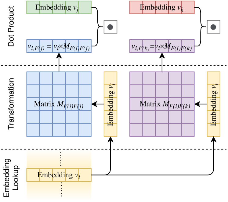
The calculation can be decomposed into 3 steps:
-
(1)
Embedding Lookup: The feature embedding vectors , and are looked up from the embedding table, and will be shared between those 2 pairs.
-
(2)
Transformation: Then is multiplied by the matrices and respectively, here we get the intermediate vector for the field , and for the field .
-
(3)
Dot Product: The final interaction terms will be a simple dot product between and , as well as and , which are the black dots showed in Fig.1.
3.1. The United Framework of Factorization Machines’ Family
FmFM have a similar design with, while extending, FM and FwFM; in this section, we deep dive into their design, explain their structure with the 3-step FmFM framework above, and figure out the fundamental relationships among these factorization machine models.
3.1.1. FM
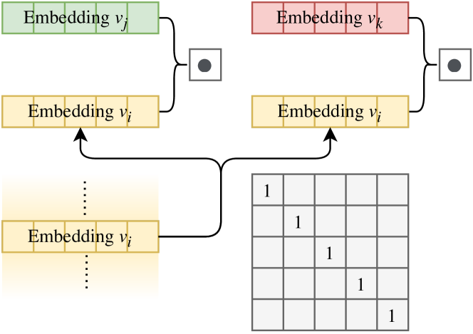
Figure 2 shows the calculation of feature interactions in FM, the difference to FmFM is that FM skip the step 2, and use the shared embedding to do the final dot product with and respectively. Since we know
we can construct an identity matrix and let all field matrices equal to . As the identity matrix shows in Fig.2, the FM actually is a special case of FmFM when all field matrices are . Since those matrices are fixed and non-trainable, we define its degree of freedom to be 0.
3.1.2. FwFM
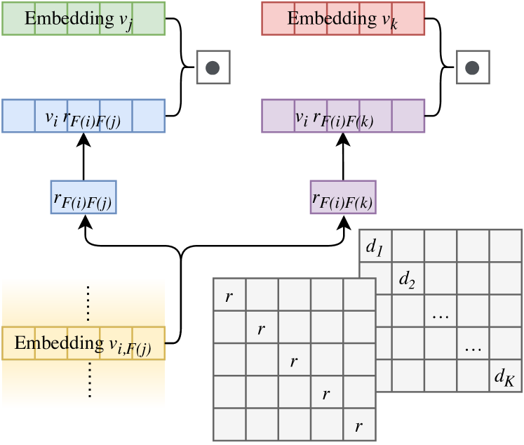
Fig.3 shows the calculation of feature interactions in FwFM. There is a change from the original definition 2, while, it is easy to know that:
Thus, we calculate the term firstly in figure 3, instead of in the original definition in Eq.2. It is clear now that the intermediate vector in step 2 is actually a scaled embedding vector:
Thus, we construct the field matrix in FwFM as a scalar matrix , which is a diagonal matrix with all its main diagonal entries equal . Its effect on the embedding vector is a scalar multiplication by . We show this matrix at the corner of Fig.3 (left one). Since the scalar is trainable, it has one more degree of freedom than FM, we define its degree of freedom as 1.
3.1.3. FvFM
We follow the clue above, and give one more freedom to the field matrix in FwFM. Let the field matrix become a diagonal matrix in which the main diagonal entries are trainable variables, instead of one single variable in FwFM, we can rewrite the intermediate vector:
where , this can be expressed more compactly by using a vector instead of the diagonal matrix, and taking the Hadamard product () of the vectors . Figure 3 demonstrates this case in the right matrix at the corner.
We name this method Field-vectorized Factorization Machines (FvFM). The FvFM have one more freedom than FwFM: the trainable parameters become a vector instead of a scalar; thus, we define its degree of freedom to be 2.
3.1.4. FmFM
Let’s revisit FmFM in figure 1. It has all the degrees of freedom of a matrix, which is 3. All the variables in those matrices are trainable, and we expect the FmFM to have a greater predictive capacity than other factorization machine models. We will evaluate this hypothesis in the next section.
Overall, we have found that FM, FwFM, FvFM are all special cases of FmFM, the only differences are their field matrices’ restrictions. According to their flexibility, we summarize them in the Table1
| Model | Field Interaction | Degree of Freedom |
| FM | Constant | 0 |
| FwFM | Scalar | 1 |
| FvFM | Vector | 2 |
| FmFM | Matrix | 3 |
3.1.5. Connections to OPNN
FmFM can also be viewed as modeling the interaction of two feature embedding vectors by a weighted outer product:
| (8) |
where , and
| (9) |
OPNN also proposed to model the feature interactions via outer product. However, FmFM is different from OPNN in the following two aspects. First, FmFM is a simple shallow model without the fully connected layers as in (Qu et al., 2016). We can use FmFM as a shallow component or a building block in any deep CTR models, like DeepFM (Guo et al., 2017). Second, we support field-specific variable embedding dimensions for features from different fields, which will be discussed in Section 4.1.
3.2. FFM and FmFM, Memorization vs Inference
Unlike other factorization machines above, FFM cannot be reformed into the FmFM framework since it has a different way to look up their feature embeddings, we demonstrate its interaction terms’ calculation in Figure 4. FFM never share the feature embedding; it always looks up the field specific embeddings from the embedding tables. Thus, there are embeddings for one single feature, which are prepared to cross other fields respectively. Those field-specific embeddings will be learned independently during the training process, and there are no restrictions among those embeddings even belonging to the same feature.
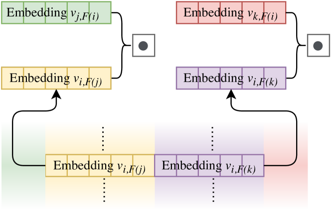
This FFM mechanism gives the model maximal flexibility to fit the data, and the huge number of embedding parameters also has incredible memorization capacity. Meanwhile, there is always a risk of over-fitting with it, even when there are billions of instances to be trained. The nature of the features’ distribution is a long tail distribution, instead of a uniform distribution, that makes the feature pairs’ distribution even more imbalanced.
Given an example in Fig.4, assume that feature pair is a high frequency combination, while is a low frequency (possibly 0 frequency, or never appeared), since and are 2 independent embeddings in the setting of FFM, thus embedding may be trained well but may not. Due to the long tail distribution of features, those high frequent features pairs may dominate the number of training data, while other low frequency features which dominate the number of features, cannot be trained well.
FmFM use shared embedding vectors, as there is only one copy for each single feature. It utilizes a transformation process to project this single embedding vector into other fields. This is basically an inference process, and those vectors are actually tied with the original embedding vector . With those field matrices, the vectors are transformable forward and backward. That is the fundamental difference between FFM and FmFM; those transformable intermediate vectors within the same feature help the model learn those low frequency feature pairs well.
Back to the example in Fig.1, even the feature pair is of low frequency, the feature embedding can still be trained well through the other high frequency feature pairs like , and the field matrix can be trained well through other feature interactions between field and field . Thus, if the low frequency feature pair occurs during evaluation or test, the intermediate vector can be inferred through .
Despite this difference between FFM and FmFM, they have more in common. An interesting observation between figure 4 and figure 1 is that, when all transformations are done, the FmFM model becomes a FFM model. We can cache those intermediate vectors and avoid matrix operations during runtime; the details will be discussed in the next section.
In contrast, FFM model cannot be reformed to a FmFM model, as we have mentioned above. Those field features embedding tables are independent, thus it is hard to compress them into one single feature embedding table and restore them when needed.
3.3. Model Complexity
The number of parameters in FM is , where accounts for the weights for each feature in the linear part and accounts for the embedding vectors for all the features . FwFM use additional parameters for each field pair so that the total number of parameters of FwFM is . The additional matrices in FmFM is as compared to FM, and it has extra parameters.
For FFM, the number of parameters is since each feature has embedding vectors. Given that usually , the number of parameters of other Factorization Machines are comparable with that of FM and significantly less than that of FFM. In Table 2 we compare the model complexity of all models mentioned so far. We also list the estimated number of parameters in the setting of section 5 for each model, which use the public data set Criteo. Those numbers can give us an intuitive impression about the size of each model. FM, FwFM, and FmFM have similar sizes while FFM have more than dozen times than others.
| Model | N of Parameters | Estimated N in Criteo Dataset |
| LR | 1.33M | |
| Poly2 | 45M | |
| FM | 14.63M | |
| FwFM | 14.63M | |
| FmFM | 14.63M | |
| FFM | 859.18M |
4. Model Optimization
In this section we present our methodologies to optimize the FmFM model. There are 3 tactics which we can devise to reduce the complexity of FmFM further. In section 4.1 we introduce the field-specific embedding dimensions, which is a unique property in FmFM; it allows us to use field specific dimensions in the embedding table, instead of a fixed length globally. In Section 4.2 we introduce the method to cache the intermediate vectors to avoid the matrix operations, which can reduce the FmFM model’s computational complexity in runtime. In Section 4.5 we introduce the method to reduce the linear terms and replace them with field specific weights.
4.1. Field-specific Embedding Dimensions
The main improvement of FM over LR model is that, FM use the embedding vector to represent each feature. In order to make the dot product, it requires the vector dimension of all feature embeddings to be the same, even though features come from different fields. The improved models like FwFM, FvFM also adopt this property. The vector dimension matters both in model complexity and model performance, the work (Pan et al., 2018) discussed this trade-off between performance and time cost, but the vector dimension can only be optimized globally.
When we utilize the matrix multiplication in FmFM, it actually does not require the field matrices to be square matrices; we can adjust the output vector length by changing the shape of the field matrix. This property gives us an another flexibility to set the field-specific lengths on-demand in the embedding table, as we show in figure 5.
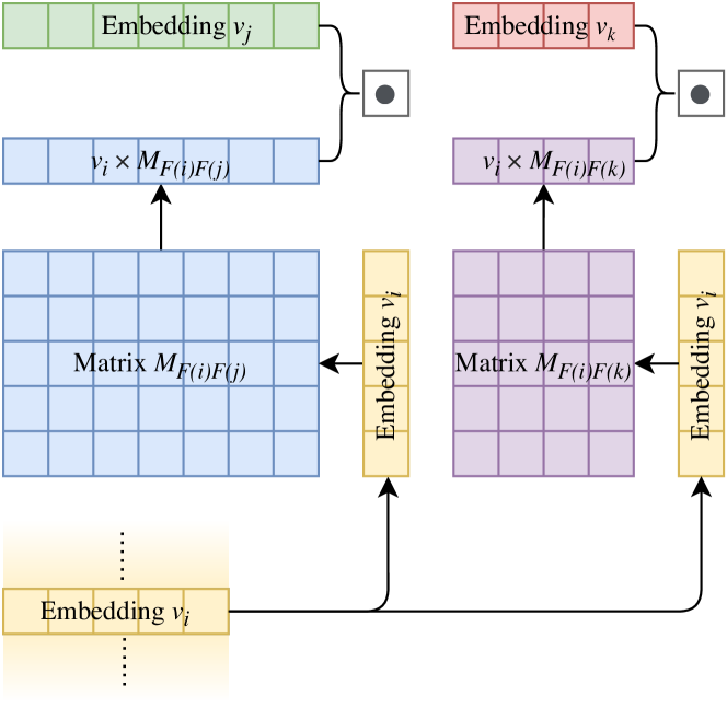
The dimension of an embedding vector determines the amount of information it can carry; this property allows us to accommodate the need for each field. For the example in Fig.5, the field may contain only 3 values (male, female, other), while another field may contain more than 1 million features. Thus, the embedding table of field may only need 5-dimension (5D), while the field may need 7D. The field matrix should be set up with a shape in . When we cross the feature between and , the matrix can transfer the 5D feature vector to a 7D vector, making it ready to do a dot product with the feature vector from field .
To optimize the field-specific embedding vector dimension without model performance loss, we propose a 2-pass method. In the first pass, we use a larger fixed embedding vector dimension for all fields, e.g. , and train the FmFM as a full model. From the full model, we learn how much information (variance) in each field, then we utilize a standard PCA dimensionality reduction to the embedding table in each field. From the experiment in Section 5.4 we found that the new dimension which contains 95% original variance is a good trade-off. With this new field specific dimension setting, we train the model in a second pass from scratch, and should get the second model without any significant performance loss, compared to the first full model.
| Feature Field ID | Emb Dim | Feat. N in Field |
| Field #01 | 3 | 62 |
| Field #02 | 8 | 113 |
| Field #03 | 5 | 125 |
| Field #04 | 7 | 50 |
| Field #05 | 9 | 223 |
| Field #06 | 8 | 147 |
| Field #07 | 6 | 99 |
| Field #08 | 5 | 78 |
| Field #09 | 8 | 103 |
| Field #10 | 3 | 8 |
| Field #11 | 5 | 31 |
| Field #12 | 3 | 56 |
| Field #13 | 6 | 81 |
| Field #14 | 8 | 1,457 |
| Field #15 | 12 | 555 |
| Field #16 | 2 | 245,195 |
| Field #17 | 11 | 166,164 |
| Field #18 | 5 | 305 |
| Field #19 | 4 | 18 |
| Field #20 | 14 | 12,054 |
| Feature Field ID | Emb Dim | Feat. N in Field |
| Field #21 | 8 | 633 |
| Field #22 | 2 | 3 |
| Field #23 | 13 | 46,329 |
| Field #24 | 14 | 5,228 |
| Field #25 | 8 | 243,452 |
| Field #26 | 13 | 3,176 |
| Field #27 | 4 | 26 |
| Field #28 | 14 | 11,744 |
| Field #29 | 10 | 225,320 |
| Field #30 | 6 | 10 |
| Field #31 | 14 | 4,726 |
| Field #32 | 12 | 2,056 |
| Field #33 | 2 | 3 |
| Field #34 | 9 | 238,638 |
| Field #35 | 4 | 16 |
| Field #36 | 6 | 15 |
| Field #37 | 12 | 67,854 |
| Field #38 | 7 | 87 |
| Field #39 | 11 | 50,940 |
Table 3 shows the optimized dimension for each field in the Criteo dataset, with the PCA method. This list shows that the range of those dimensions are huge which from 2 to 14, and most of the dimensions are less than 10. The average is only 7.72, which is less than the optimal setting in the FwFM. With keeping most variance from the dataset, the lower average dimension means the model has fewer parameters, requires less memory.
4.2. Intermediate Vectors Cache
FmFM is a lower complexity model than FFM, in the number of parameters; however it requires expensive matrix operations in the transformation step. In table 4, we list the number of Floating Point Operations (FLOPs) for each model111We use the following values to estimate the FLOPs: , denotes the number of nodes in the hidden layers of DNN, denotes the number of hidden layers in DNN, denotes the dimension of embedding vectors in the new space in AutoInt, and denotes the sparsity rate of the FwFM and DNN component in DeepLight., and estimate it with typical settings.
| Model | Floating Point Operations | Estimated # |
| LR | 78 | |
| Poly2 | 1,560 | |
| FM | 1,920 | |
| FwFM | 25,272 | |
| FFM | 24,531 | |
| FmFM | 403,923 | |
| FmFM(cached) | 24,531 | |
| FmFM(cached & 95% variance) | 8,960 | |
| Wide & Deep | ~500,000 | |
| Deep & Cross | ~510,000 | |
| DeepFM | ~246,000 | |
| xDeepFM | ~150,000,000 | |
| AutoInt | ~28,000,000 | |
| FiBiNET | ~10,000,000 | |
| DeepLight | ~102,000 |
Among those Factorization Machine models, the FmFM needs the most operations to accomplish its calculation, which is about times as FwFM and FFM, but still faster than most DNN models. In section 3.2, we have shown that a FmFM model can be transformed into a FFM model, by caching all intermediate vectors. In this sense, we can reduce its number of operations to the same magnitude as FM and FFM, which is almost 20 times faster.
4.3. Embedding Dimension and Cache Optimization Combined
When we combine the field-specific embedding dimensional optimization and the cache optimization, the inference speed can be much faster, and the required memory can be reduced significantly. This benefits from another property of FmFM - the interaction matrices are symmetrical, which means
| (10) |
We have a proof for this lemma in the Appendix.
Thus, we can choose to cache those intermediate vectors which have lower field dimensions, and dot-product with the other feature vectors during inference. For example, in the setting of table 3, two features and are from field #16 and #28 respectively. With this property, when we calculate the interaction between and , we can cache either or .
Since the field matrix has a shape of , the former one increased the dimension from 2 (field #16) to 14 (intermediate vector), then dot-product with whose dimension is also 14. It costs 14 units of memory for the intermediate vectors cache, and takes FLOPs during inference. By contrast, the latter one reduces the dimension from 14 (field #28) to 2 (intermediate vector), then dot-product with whose dimension is also 2. It costs 2 units of memory for the intermediate vectors cache, and takes FLOPs during inference. In this single field pair, the optimized cache with field-specific embedding dimensions can save 7 times memory and time without any precision loss.
With those two optimization techniques combined, the FmFM model’s time complexity is reduced drastically; in table 4, we estimate that the optimized model only takes 8,960 FLOPs, which is only about 1/3 of FFM. In the section5.4, we will show that this optimized model can achieve the same performance as the full model.
4.4. Soft Pruning
The field-specific embedding dimensions also act in a role similar to pruning actually; while traditional pruning such as DeepLight (Deng et al., 2020) gives a binary decision to keep or drop a field or a field pair, the field-specific embedding dimensions give us a new way to determine the importance of each field and field pair on-demand, and assign each field a factor to represent its importance. For example, in the FmFM model of Table3, the cross field #17 and #20 is a high strength pair; it takes 11 units of cache and FLOPs during inference; in contrast, a low strength pair, field #18 and #22, only takes 2 units of cache and FLOPs.
When we drop a field pair in the traditional pruning, its signal was lost totally; while in this method, a field pair still keeps the major information with minimal cost. It is a soft version of pruning, which is similar to Softmax. It is more efficient and sees less performance drop during soft pruning.
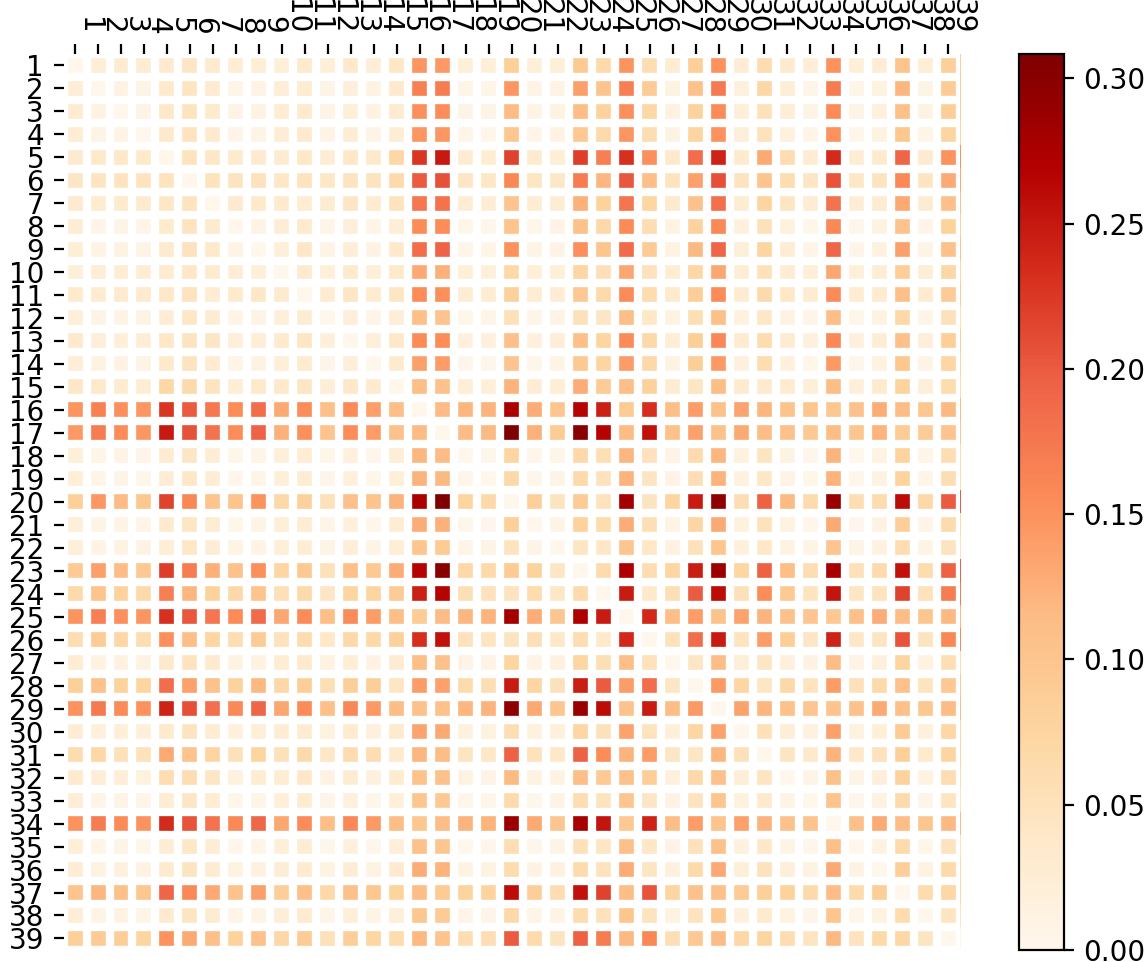
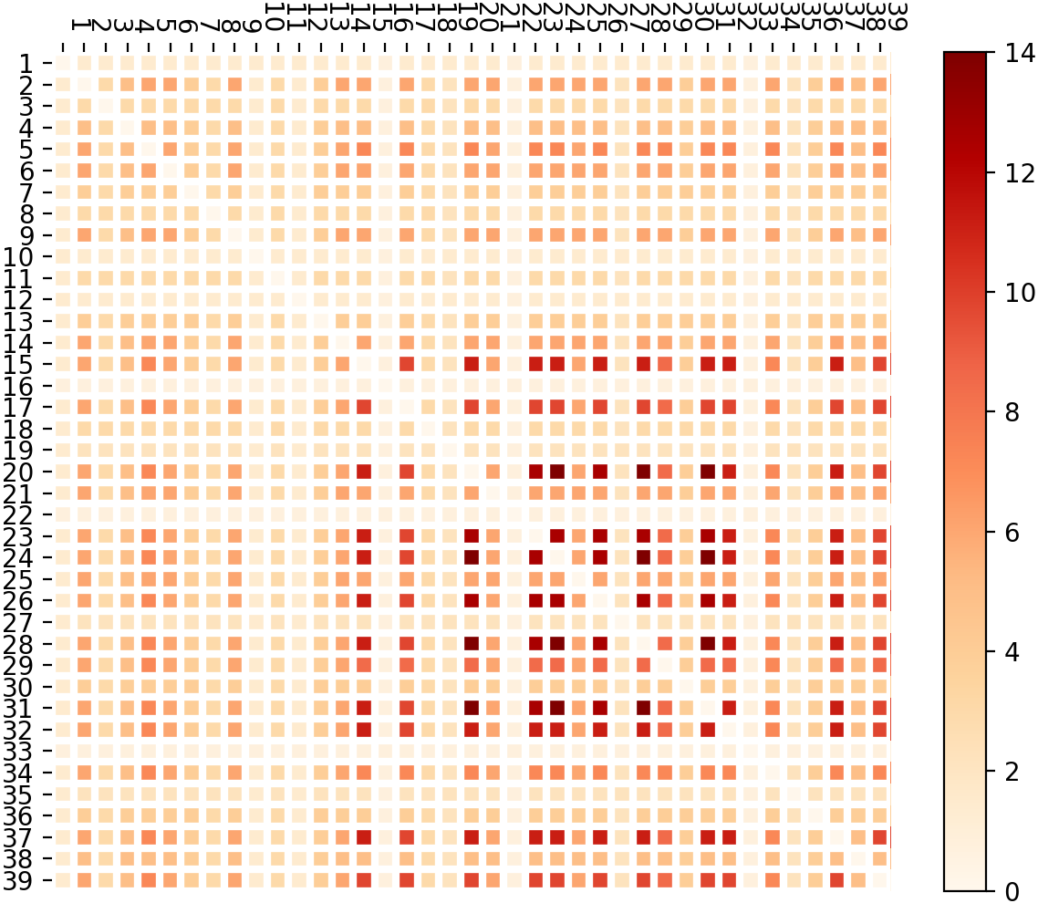
Figure 6 shows a heat-map of mutual information scores between field pairs and labels in the Criteo dataset, which represents the strength of field pairs in prediction. Figure 7 shows the cross field dimensions, which is the lower dimension between two fields (explanation in Section 4.3); it represents the parameters and computational cost for each field pair. Obviously, these two heat-maps are highly related to each other, which means the optimized FmFM model allocates more parameters and more computation on those higher strength field pairs, and fewer parameters and less computation on lower strength field pairs.
4.5. Linear Terms
There is a linear part in Eq.8:
| (11) |
which requires an extra scalar to be learned for each feature. However the learned embedding vector should contain more information, and the weight can be learned from by a simple dot product. Another benefit from the learned is that, it can help to learn the embedding vector from the linear part.
We follow the method from the work of (Pan et al., 2018), by learning a field specific vector so that all features from the same field will share the same linear weight vector. Then the linear terms can be rewritten to:
| (12) |
We apply this linear term optimization to FwFM, FvFM and FmFM by default in the rest of the paper.
5. Experiments
In this section we present our experimental evaluation results. We will first describe the data sets and implementation details in Section 5.1 and 5.2 respectively. In Section 5.3 we compare FmFM with other baseline models like LR, FM, FwFM and FFM, as well as the state-of-the-art methods like Wide & Deep, Deep & Cross network, xDeepFM, AutoInt, FiBiNET and DeepLight. In Section 5.4, we did a few experiment on the Criteo dataset and observe the model performance change when we apply the field-specific dimension in embedding.
5.1. Data sets
We use 2 public data sets to evaluate our model performance:
-
(1)
The first one is the Criteo CTR data set; it is a well-know benchmark data set which used for the Criteo Display Advertising Challenge (Labs, 2014). The Criteo data set is already label balanced, the positive to the negative ratio is about 1:3. There are 45 million samples and each sample has 13 numerical fields and 26 categorical fields.
-
(2)
The second data set is the Avazu CTR data set; it was used in the Avazu CTR prediction competition, which predicts whether a mobile ad will be clicked. The positive to the negative ratio in the Avazu data set is about 1:5. There are 40 million samples and each sample has 23 categorical fields.
We follow those existing works (Guo et al., 2017; Lian et al., 2018; Shan et al., 2016; Wang et al., 2017; Zhang et al., 2016; Zhou et al., 2018b; Deng et al., 2020; Song et al., 2018), for each data set, we split it into 3 parts randomly, 80% for training, 10% for validation, and 10% for testing. 222Some of those works split 90%:10% for just training and testing, but we adopt the strict one with validation set and less training set.
Regarding to those numerical features in the Criteo data set, we adopt the log transformation of if , which proposed by the winner of the Criteo competition333https://www.csie.ntu.edu.tw/ r01922136/kaggle-2014-criteo.pdf to normalize the numerical features. This method was also used by (Deng et al., 2020) and (Song et al., 2018). Regarding the date/hour feature in the Avazu data set, we transfer it into 2 features: day_of_week(0-6) and hours(0-23) to consume the feature better.
We also remove those infrequent features that are less than a threshold in both data sets and replace their values with the default ”unknown” feature in that field. We set the threshold to 8 for the Criteo data set, and to 5 for the Avazu data set.
The statistics of the normalized data sets are shown in Table 5.
| Data set | Samples | Fields | Features | Pos:Neg | |
| Criteo | Train | 36,672,493 | 39 | 1,327,180 | ~1:3 |
| Validation | 4,584,062 | ||||
| Test | 4,584,062 | ||||
| Avazu | Train | 32,343,173 | 23 | 1,544,257 | ~1:5 |
| Validation | 4,042,897 | ||||
| Test | 4,042,897 | ||||
5.2. Experiment Setup
We have implemented the LR (logistic regression) and all factorization machine models (FM, FwFM, FFM, FvFM and FmFM) with Tensorflow.444We open-sourced the training code and the feature extraction code at
https://github.com/VerizonMedia/FmFM. We follow the implementation of LR and FM in (Qu
et al., 2016), and implement FFM, FwFM following the work (Pan
et al., 2018).
We evaluate all models performance by AUC (Area Under the ROC Curve) and Log Loss on the test set. It is noticeable that a slightly higher AUC or lower Log Loss at 0.001-level is regarded a significant improvement for CTR prediction task, which has also been pointed out in existing works (Song et al., 2018; Cheng et al., 2016; Wang et al., 2017).
For those state-of-the-art models, they are all DNN models and may need more hyper-parameters tuning, we pull their performance (AUC and Log Loss) from their original papers, in order to keep their results optimal. It is fair to compare our results with theirs, since we use more strict data splittings; while their implementations may have slight differences, e.g. feature processing, optimizer (Adam or Adagrad), we list their results just for reference. The Deep & Cross Network is an exception, since their paper only listed the Log Loss but not AUC. Thus, we implemented their model and got a similar performance.
5.3. Performance Comparisons
In this section we will conduct performance evaluation for FmFM. We will compare it with LR, FM, FwFM and FFM on the two data sets mentioned above. We always use the full size model to compare in the results; that means we don’t use any optimization methods mentioned in Section 4. For the parameters such as regularization coefficient , and learning rate in all models, we select those which lead to the best performance on the validation set and then use them in the evaluation on the test set. Experiment results can be found in Table 6 for the Criteo data set, and Table 7 for the Avazu data set.
| Models | AUC | Log Loss (Test Set) | ||
| Training | Validation | Test | ||
| LR | 0.7930 | 0.7918 | 0.7917 | 0.4582 |
| FM | 0.8142 | 0.8075 | 0.8075 | 0.4441 |
| FFM | 0.8230 | 0.8103 | 0.8103 | 0.4414 |
| FwFM | 0.8191 | 0.8092 | 0.8092 | 0.4426 |
| FvFM(ours) | 0.8192 | 0.8102 | 0.8101 | 0.4417 |
| FmFM(ours) | 0.8183 | 0.8109 | 0.8109 | 0.4410 |
| Deep & Cross | 0.8244 | 0.8118 | 0.8118 | 0.4413 |
| Wide & Deep | - | - | 0.7981 | 0.4677 |
| DeepFM | - | - | 0.8007 | 0.4508 |
| xDeepFM | - | - | 0.8052 | 0.4418 |
| AutoInt | - | - | 0.8061 | 0.4454 |
| FiBiNET | - | - | 0.8103 | 0.4423 |
| DeepLight | - | - | 0.8123 | 0.4395 |
| Models | AUC | Log Loss (Test Set) | ||
| Training | Validation | Test | ||
| LR | 0.7526 | 0.7521 | 0.7517 | 0.3953 |
| FM | 0.7744 | 0.7696 | 0.7695 | 0.3857 |
| FFM | 0.8012 | 0.7761 | 0.7761 | 0.3826 |
| FwFM | 0.7822 | 0.7730 | 0.7731 | 0.3835 |
| FvFM(ours) | 0.7836 | 0.7732 | 0.7733 | 0.3834 |
| FmFM(ours) | 0.7943 | 0.7764 | 0.7763 | 0.3822 |
| Deep & Cross | 0.8109 | 0.7825 | 0.7826 | 0.3791 |
| AutoInt | - | - | 0.7752 | 0.3823 |
| Fi-GNN | - | - | 0.7762 | 0.3825 |
| FGCNN+IPNN | - | - | 0.7883 | 0.3746 |
| DeepLight | - | - | 0.7897 | 0.3748 |
We observe that FvFM and FmFM can achieve better performance than LR, FM, and FwFM on both data sets, which is in our expectation. Surprisingly, the FmFM can achieve better performance than FFM constantly in both test sets. As we mentioned before, even though FFM is a model dozens times larger than FmFM, our FmFM model still get the best AUC in the test set among all shallow models. Additionally, if we compare the differences in AUC between training and test, we found that the is the lowest one among those factorization machine models, which affirms our hypothesis in section 3.2: those low frequency features are also trained well with the help of the interaction matrix, and this mechanism helps FmFM to avoid over-fitting.
5.4. Embedding Dimension Optimization
In this part we implement the method described in 4.1, whereby we have a full size model, we can extract its embedding tables for each field, then we utilize a standard PCA dimensionality reduction. Here we do several experiments and compare how the dimensionality reduction impact the model performance, and try to find a trade-off between the model size, speed and its performance.
We use the full size FmFM model from experiment 5.3 on the Criteo data set to evaluate our metrics. We keep 99%, 97%, 95%, 90%, 85% and 80% variance in PCA dimensionality reduction respectively, and estimate the average embedding dimensions and float operations (FLOPs, with cached intermediate vectors). With the new dimensions setting, we train those FmFM models the second pass respectively, and observe the AUC and Log Loss change in test set.
Table 8 shows the summary of experiments. The average embedding dimension was reduced significantly when we keep less variance from PCA: there is only less than 1/2 embedding dimensions and 1/3 computation cost when we keep 95% variance, while there is no significant change on the model’s performance compare to the full size model. Thus, 95% variance is a good trade-off when we optimize the embedding dimensions in FmFM.
| Variance % | Emb Dim (Average) | FLOPs Estimated # | AUC (Test Set) | Log Loss (Test Set) |
| Full | 16(100%) | 24,531(100%) | 0.8109 | 0.4410 |
| 99% | 10.56(66.0%) | 12,884(52.5%) | 0.8109 | 0.4410 |
| 97% | 8.69(54.3%) | 10,280(41.9%) | 0.8107 | 0.4411 |
| 95% | 7.72(48.2%) | 8,960(36.5%) | 0.8108 | 0.4411 |
| 90% | 6.26(39.1%) | 7,202(29.4%) | 0.8103 | 0.4415 |
| 85% | 3.82(23.9%) | 4,716(19.2%) | 0.8084 | 0.4432 |
| 80% | 3.36(21.0%) | 4,392(17.9%) | 0.8080 | 0.4436 |
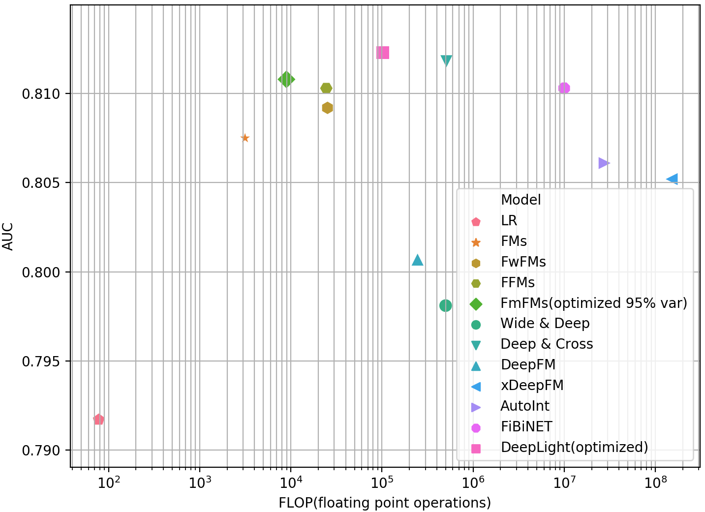
Figure 8 shows these models’ performance (in AUC) and their computational complexity (in FLOPs). As a shallow model, the optimized FmFM model gets higher AUC as well as lower FLOPs, compared with all the baseline models except Deep & Cross and DeepLight. While its computational cost is much lower than these two complex models which ensembled DNN module and shallow module, its FLOPs is only 1.76% and 8.78% of them, respectively. The lower FLOPs makes it preferable when the computation latency is strictly limited, which is the common scenario in the real-time online ads CTR prediction and recommender systems.
6. Conclusion and Further Works
In conclusion, we propose a novel approach FmFM to model the interactions of field pairs as a matrix. We prove that FmFM is a unified framework of factorization machine model family, in which both FM and FwFM can be treated as special cases. We devise a few optimizations to FmFM, including field-specific embedding dimensions and caching intermediate vectors. These optimizations make the FmFM lightweight and faster during inference, taking only thousands of floating-point operations to make a prediction. We have done comprehensive experiments to verify the effectiveness and efficiency of the proposed model. It achieves state-of-the-art performance among all shallow models, including FM, FFM and FwFM, and its performance is even comparable to those complex DNN models.
With regard to future work, there are a few potential research directions:
-
•
The FmFM is still a linear model, since the field interaction are matrices, and embedding vectors are transformed linearly. We can introduce the non-linear layers to the field interaction and let the model become a non-linear model, which is more flexible.
-
•
All the factorization machine models are actually Degree-2 models, which allows up to 2 fields interactions. This restriction is majorly because the dot product. In the future, we can introduce the 3D tensor and allows the 3 fields interaction, or even higher ranks. This work may require more model optimization since there are too much Degree-3 interactions.
-
•
We can combine the DNN models like the Wide and Deep (Cheng et al., 2016), DeepFM (Guo et al., 2017), DeepLight (Deng et al., 2020), and try FmFM as a building block in DNN models to further improve their performances. We believe this method should be more competitive in the model performance, when compare to those deep learning based models in Section 2.
References
- (1)
- Aharon et al. (2013) Michal Aharon, Natalie Aizenberg, Edward Bortnikov, Ronny Lempel, Roi Adadi, Tomer Benyamini, Liron Levin, Ran Roth, and Ohad Serfaty. 2013. OFF-set: one-pass factorization of feature sets for online recommendation in persistent cold start settings. In Proceedings of the 7th ACM Conference on Recommender Systems. ACM, 375–378.
- Chang et al. (2010) Yin-Wen Chang, Cho-Jui Hsieh, Kai-Wei Chang, Michael Ringgaard, and Chih-Jen Lin. 2010. Training and testing low-degree polynomial data mappings via linear SVM. Journal of Machine Learning Research 11, Apr (2010), 1471–1490.
- Chapelle et al. (2015) Olivier Chapelle, Eren Manavoglu, and Romer Rosales. 2015. Simple and scalable response prediction for display advertising. ACM Transactions on Intelligent Systems and Technology (TIST) 5, 4 (2015), 61.
- Cheng et al. (2016) Heng-Tze Cheng, Levent Koc, Jeremiah Harmsen, Tal Shaked, Tushar Chandra, Hrishi Aradhye, Glen Anderson, Greg Corrado, Wei Chai, Mustafa Ispir, et al. 2016. Wide & deep learning for recommender systems. In Proceedings of the 1st Workshop on Deep Learning for Recommender Systems. ACM, 7–10.
- Deng et al. (2020) Wei Deng, Junwei Pan, Tian Zhou, Aaron Flores, and Guang Lin. 2020. DeepLight: Deep Lightweight Feature Interactions for Accelerating CTR Predictions in Ad Serving. Proceedings of the 14th ACM international conference on Web search and data mining (2020).
- Deng et al. (2017) Xiaotie Deng, Paul Goldberg, Yang Sun, Bo Tang, and Jinshan Zhang. 2017. Pricing ad slots with consecutive multi-unit demand. Autonomous Agents and Multi-Agent Systems 31, 3 (2017), 584–605.
- Guo et al. (2017) Huifeng Guo, Ruiming Tang, Yunming Ye, Zhenguo Li, and Xiuqiang He. 2017. DeepFM: A Factorization-Machine based Neural Network for CTR Prediction. arXiv preprint arXiv:1703.04247 (2017).
- He and Chua (2017) Xiangnan He and Tat-Seng Chua. 2017. Neural Factorization Machines for Sparse Predictive Analytics. (2017).
- Juan et al. (2017) Yuchin Juan, Damien Lefortier, and Olivier Chapelle. 2017. Field-aware factorization machines in a real-world online advertising system. In Proceedings of the 26th International Conference on World Wide Web Companion. International World Wide Web Conferences Steering Committee, 680–688.
- Juan et al. (2016) Yuchin Juan, Yong Zhuang, Wei-Sheng Chin, and Chih-Jen Lin. 2016. Field-aware factorization machines for CTR prediction. In Proceedings of the 10th ACM Conference on Recommender Systems. ACM, 43–50.
- Koren et al. (2009) Yehuda Koren, Robert Bell, and Chris Volinsky. 2009. Matrix factorization techniques for recommender systems. Computer 42, 8 (2009).
- Labs (2014) Criteo Labs. 2014. Display Advertising Challenge. https://www.kaggle.com/c/criteo-display-ad-challenge
- Lian et al. (2018) Jianxun Lian, Xiaohuan Zhou, Fuzheng Zhang, Zhongxia Chen, Xing Xie, and Guangzhong Sun. 2018. xDeepFM: Combining Explicit and Implicit Feature Interactions for Recommender Systems. 2018 ACM SIGKDD International Conference on Knowledge Discovery and Data Mining.
- McMahan et al. (2013) H Brendan McMahan, Gary Holt, David Sculley, Michael Young, Dietmar Ebner, Julian Grady, Lan Nie, Todd Phillips, Eugene Davydov, Daniel Golovin, et al. 2013. Ad click prediction: a view from the trenches. In Proceedings of the 19th ACM SIGKDD international conference on Knowledge discovery and data mining. ACM, 1222–1230.
- Pan et al. (2019) Junwei Pan, Yizhi Mao, Alfonso Lobos Ruiz, Yu Sun, and Aaron Flores. 2019. Predicting different types of conversions with multi-task learning in online advertising. In Proceedings of the 25th ACM SIGKDD International Conference on Knowledge Discovery & Data Mining. 2689–2697.
- Pan et al. (2018) Junwei Pan, Jian Xu, Alfonso Lobos Ruiz, Wenliang Zhao, Shengjun Pan, Yu Sun, and Quan Lu. 2018. Field-weighted Factorization Machines for Click-Through Rate Prediction in Display Advertising. Proceedings of the 2018 World Wide Web Conference on World Wide Web - WWW ’18 (2018). https://doi.org/10.1145/3178876.3186040
- Qu et al. (2016) Yanru Qu, Han Cai, Kan Ren, Weinan Zhang, Yong Yu, Ying Wen, and Jun Wang. 2016. Product-based neural networks for user response prediction. In 2016 IEEE 16th International Conference on Data Mining (ICDM). IEEE, 1149–1154.
- Rendle (2010) Steffen Rendle. 2010. Factorization machines. In Data Mining (ICDM), 2010 IEEE 10th International Conference on. IEEE, 995–1000.
- Rendle (2012) Steffen Rendle. 2012. Factorization machines with libfm. ACM Transactions on Intelligent Systems and Technology (TIST) 3, 3 (2012), 57.
- Richardson et al. (2007) Matthew Richardson, Ewa Dominowska, and Robert Ragno. 2007. Predicting clicks: estimating the click-through rate for new ads. In Proceedings of the 16th international conference on World Wide Web. ACM, 521–530.
- Shan et al. (2016) Ying Shan, T Ryan Hoens, Jian Jiao, Haijing Wang, Dong Yu, and JC Mao. 2016. Deep Crossing: Web-scale modeling without manually crafted combinatorial features. In Proceedings of the 22nd ACM SIGKDD International Conference on Knowledge Discovery and Data Mining. ACM, 255–262.
- Song et al. (2018) Weiping Song, Chence Shi, Zhiping Xiao, Zhijian Duan, Yewen Xu, Ming Zhang, and Jian Tang. 2018. AutoInt: Automatic Feature Interaction Learning via Self-Attentive Neural Networks. CIKM ’19: Proceedings of the 28th ACM International Conference on Information and Knowledge Management (2018).
- Sun et al. (2012) Yang Sun, Yunhong Zhou, Ming Yin, and Xiaotie Deng. 2012. On the convergence and robustness of reserve pricing in keyword auctions. In Proceedings of the 14th Annual International Conference on Electronic Commerce. 113–120.
- Wang et al. (2017) Ruoxi Wang, Bin Fu, Gang Fu, and Mingliang Wang. 2017. Deep & Cross Network for Ad Click Predictions. arXiv preprint arXiv:1708.05123 (2017).
- Yang et al. (2011) Sun Yang, Zhou Yunhong, and Deng Xiaotie. 2011. Optimal Reserve Prices in Weighted GSP Auctions: Theory and Experimental Methodology. In 7th Ad Auction Workshop in conjunction with the 12th ACM Conference on Electronic Commerce.
- Zhang et al. (2016) Weinan Zhang, Tianming Du, and Jun Wang. 2016. Deep learning over multi-field categorical data. In European conference on information retrieval. Springer, 45–57.
- Zhou et al. (2018a) Guorui Zhou, Ying Fan, Runpeng Cui, Weijie Bian, Xiaoqiang Zhu, and Kun Gai. 2018a. Rocket launching: A universal and efficient framework for training well-performing light net. In Proceedings of the AAAI Conference on Artificial Intelligence, Vol. 32.
- Zhou et al. (2018b) Guorui Zhou, Xiaoqiang Zhu, Chenru Song, Ying Fan, Han Zhu, Xiao Ma, Yanghui Yan, Junqi Jin, Han Li, and Kun Gai. 2018b. Deep interest network for click-through rate prediction. In Proceedings of the 24th ACM SIGKDD International Conference on Knowledge Discovery & Data Mining. 1059–1068.
Appendix A Math Proof
Lemma A.1.
Given two row vectors and whose lengths are and respectively, there is a matrix , then:
| (13) |
where denotes matrix multiplication, and denotes dot product.
Proof.
Since is a scalar, we denote it as , and the dot product can be rewrite to a matrix multiplication, we rewrite the left of the equation:
| (14) |
while the transpose of a scalar equals to itself:
| (15) |
Hence, the left equals the right. ∎