Controlling nonlinear dynamical systems into arbitrary states using machine learning

Abstract

We propose a novel and fully data driven control scheme which relies on machine learning (ML). Exploiting recently developed ML-based prediction capabilities of complex systems we demonstrate that nonlinear systems can be forced to stay in arbitrary dynamical target states coming from any initial state. We outline our approach using the examples of the Lorenz and the Rössler system and show how these systems can very accurately be brought not only to periodic but also to e.g. intermittent and different chaotic behavior. Having this highly flexible control scheme with little demands on the amount of required data on hand, we briefly discuss possible applications that range from engineering to medicine.

The possibility to control nonlinear chaotic systems into stable states has been a remarkable discovery [1, 2]. Based on the knowledge of the underlying equations, one can force the system from a chaotic state into a fixed point or periodic orbit by applying an external force. This can be achieved based on the pioneering approaches by Ott et. al [1] or Pyragas [3]. In the former, a parameter of the system is slightly changed when it is close to an unstable period orbit in phase space, while the latter continuously applies a force based on time delayed feedback. There have been many extensions of those basic approaches (see e.g. [4] and references therein) including ”anti-control” schemes [5], that break up periodic or synchronized motion. But all of them do not allow to control the system into well-specified, yet more complex target states such as chaotic or intermittent behavior. Further, these methods either require exact knowledge about the system, i.e. the underlying equations of motion, or rely on phase space techniques for which very long time series are necessary.
In recent years, tremendous progress has been made in the prediction of nonlinear dynamical systems by means of machine learning (ML). It has been demonstrated that not only exact short term predictions over several Lyapunov times become possible, but also the long term behavior of the system (its ”climate”) can be reproduced with unexpected accuracy [6, 7, 8, 9, 10, 11, 12] – even for very high-dimensional systems [13, 14]. While several ML techniques have successfully been applied to time series prediction, reservoir computing (RC) [15, 16] can be considered as the so far best approach as it combines often superior performance with intrinsic advantages like smaller network size, higher robustness, fast and comparably transparent learning [17] and the prospect of highly efficient hardware realizations [18, 19, 20].
Combining now ML-based predictions of complex systems with manipulation steps, we propose in this Letter a novel, fully data-driven approach for controlling nonlinear dynamical systems. In contrast to previous methods, this allows to obtain a variety of target states including periodic, intermittent and chaotic ones. Furthermore, we do not require the knowledge of the underlying equations. Instead, it is sufficient to record some history of the system that allows the machine learning method to be sufficiently trained. As previously outlined [21], an adequate learning requires orders of magnitude less data than phase space methods.
In this work, the prediction is solely performed with RC [22], where the input data $\textbf{u}(t)$ is mapped into a higher dimensional state $\textbf{r}(t)$ through the dynamics of a fixed random reservoir A. The reservoir state $\textbf{r}(t)$ is updated according to $\textbf{r}(t+\Delta{t})=\alpha\textbf{r}(t)+tanh(\textbf{A}\textbf{r}(t)+\textbf{W}_{in}\textbf{u}(t))$, where $\textbf{W}_{in}$ denotes the fixed input mapping function. Output $\textbf{v}(t+\Delta{t})$ is created by mapping back $\textbf{r}(t)$ using a linear output function $\textbf{W}_{out}$ such that $\textbf{v}(t)=\textbf{W}_{out}(\mathbf{\tilde{r}}(t),\textbf{P})=\textbf{P}\mathbf{\tilde{r}}(t)$, where $\mathbf{\tilde{r}}=\{\mathbf{r},\mathbf{r}^{2}\}$. The matrix P is determined in the training process. Replacing $\textbf{u}(t)$ in the tanh activation function above by $\textbf{P}\mathbf{\tilde{r}}(t)$ allows to create predictions of arbitrary length due to the recursive equation for the reservoir states $\textbf{r}(t)$. Further details are presented in the supplementary material.

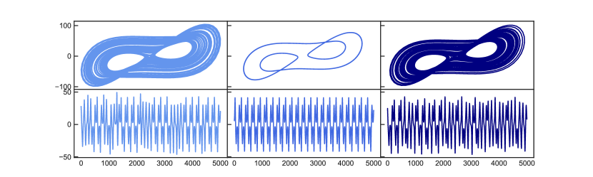
Figure 1: Periodic to chaotic control. Top: 2D attractor representation in the x-y plane. Bottom: X coordinate time series. Left plots show the original chaotic state which changes to a periodic state (middle) after tuning the order parameter. After applying the control mechanism, the system is forced into a chaotic state again (right).

The control of complex nonlinear dynamical system is studied on the example of the Lorenz system [23], which is a model for atmospheric convection. Depending on the choice of parameters, the system exhibits e.g. periodic, intermittent or chaotic behavior. In contrast to classical approaches, our method relies on a good prediction of the system based on reservoir computing or other suitable machine learning techniques. The setup for the control procedure is then the following: We simulate the Lorenz system for a certain parameter set $\bm{\pi}$ by integrating its differential equations $\dot{f}(\textbf{u},\bm{\pi})$ and train RC on it. Here, $\textbf{u}=(x,y,z)^{T}$ and the equations read

$$\dot{x}=\sigma(y-x);\ \ \dot{y}=x(\rho-z)-y;\ \ \dot{z}=xy-\beta z\ ,$$ (1)

while $\bm{\pi}\equiv(\sigma,\rho,\beta)$. Then the parameters are shifted to $\bm{\pi^{*}}$ such that the system behavior changes. In order to bring the system back to the desired original state, a correction force defined as $\textbf{F(t)}=K(\textbf{u}(t)-\textbf{v}(t))$ is applied. Now, $\textbf{u}(t)$ represents the coordinates of the system with changed parameters, whereas $\textbf{v}(t)$ denotes the theoretical coordinates of the predicted trajectory and $K$ scales the magnitude of the force and is set to $K=25$ for all examples. The coordinates $\textbf{u}(t+\Delta{t})$ for the next time step are obtained by solving the equations of the Lorenz system including the force

$$\textbf{u}(t+\Delta{t})=\int_{t}^{t+\Delta{t}}(\dot{f}(\textbf{u}(\tilde{t}),\bm{\pi^{*}})+\textbf{F}(\tilde{t}))d\tilde{t},$$ (2)

however, still using the new parameters $\bm{\pi^{*}}$, which lead to an undesired state of the system if the control force $\textbf{F}(t)$ is not applied.

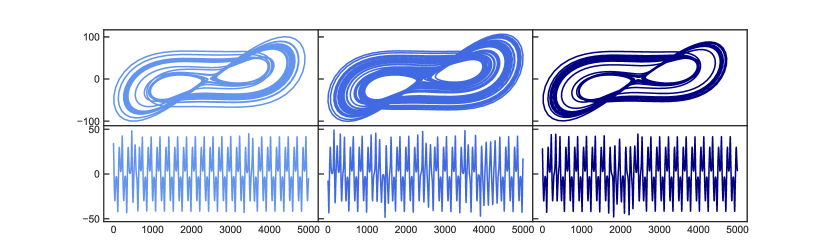
Figure 2: Chaotic to intermittent control. Top: 2D attractor representation in the x-y plane. Bottom: X coordinate time series. Left plots show the original intermittent state which changes to a chaotic state (middle) after tuning the order parameter. After applying the control mechanism, the system is forced into an intermittent state again (right).

Figure 1 shows the results for the Lorenz system originally (left side) being in a chaotic regime ($\bm{\pi}=[\sigma=10.0,\rho=167.2,\beta=8/3]$), which then changes to periodic behavior (middle) after $\rho$ is changed to $\rho=166$. Then, the control mechanism is activated and the resulting attractor again resembles the original chaotic state (left). While ’chaotification’ of periodic states has been achieved in the past, the resulting attractor generally did not correspond to a certain specified target state but just exhibited some chaotic behavior. Since we would like to not only rely on a visual assessment, we characterize the attractors using quantitative measures. First, we calculate the largest Lyapunov exponent, which quantifies the temporal complexity of the trajectory, where a positive value indicates chaotic behavior. Second, we use the correlation dimension to asses the structural complexity of the attractor. Based on the two measures, the dynamical state of the system can be sufficiently specified for our analysis. Both techniques are described in the supplementary material. Because a single example is not sufficiently meaningful, we perform our analysis statistically by evaluating 100 random realizations of the system at a time. The term ’random realization’ refers to different random drawings of the reservoir A and the input mapping $\textbf{W}_{in}$. The first line in Table 1 shows the respective statistical results for the setup shown in Figure 1. The largest Lyapunov exponent of the original chaotic system $\lambda_{orig}=0.851$ significantly reduces to $\lambda_{changed}=0.080$ when the parameter change drives the system into a periodic state. After the control mechanism is switched on, the value for the resulting attractor moves back to $\lambda_{controlled}=0.0841$ and thus is within one standard deviation from its original value. Same applies to the correlation dimension, which resembles its original value after control very well.

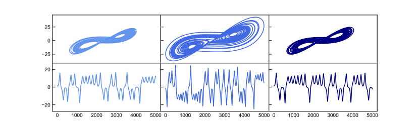
Figure 3: Chaotic to chaotic control. Top: 2D attractor representation in the x-y plane. Bottom: X coordinate time series. Left plots show the original chaotic state which changes to a different chaotic state (middle) after tuning the order parameter. After applying the control mechanism, the system is forced into the initial chaotic state again (right).

Since there is a clear distinction between the chaotic- and the periodic state, with the latter being simple in terms of its dynamics, the next step is to control the system between more complex dynamics. Therefore, we start simulate the Lorenz system again with parameters $\bm{\pi}=[\sigma=10.0,\rho=166.15,\beta=8/3]$ that lead to intermittent behavior [24]. This is shown in Fig 2 on the left. Now $\rho$ is changed to $\rho=167.2$, which results in a chaotic state (middle plots). The control mechanism is turned on and the resulting state shows again the intermittent behavior (right plots) as in the initial state. This is particularly visible in the lower plots where only the X coordinate is shown. While the trajectory mostly follows a periodic path, it is interrupted by irregular burst that occur from time to time. It is remarkable that bursts do not seem to occur more often given the chaotic dynamics of the underlying equations and parameter setup. However, the control works so well that it exactly enforces the desired dynamics. This observation can again be confirmed by looking at the statistical results in Table 1.

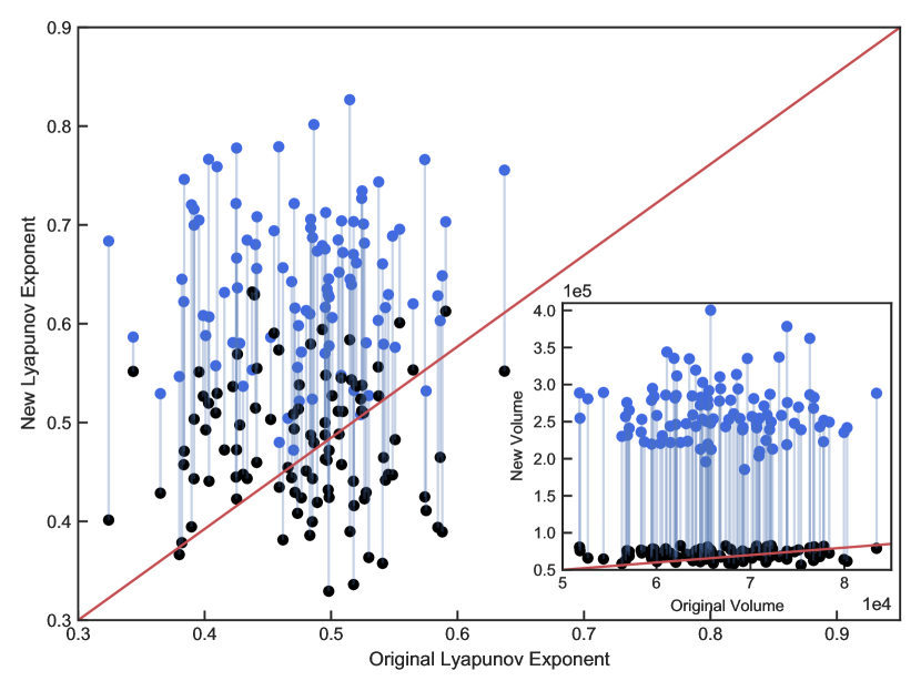
Figure 4: Chaotic to chaotic control ($\rho$ changed). Values on the x-axis denote the largest Lyapunov exponent $\lambda_{max}$ of the original system state before parameter change for $N=100$ random realizations. Y-axis reflects the values for $\lambda_{max}$ after parameters changed from $\rho=28$ to $\rho=50$. The blue dots correspond to the uncontrolled systems, while the black dots represent the controlled systems. Inlay plot shows the same for the volume of the attractor.

Table 1: Statistical simulation over $N=100$ random realizations of the systems evaluated in terms of the mean values of the largest Lyapunov exponent and the correlation dimension with corresponding standard deviations. The subscript orig denotes the initial state of the system, while changed refers to the new state after parameters changed and controlled means the system controlled back into the original state. The description left to the arrow is the original state that also will be achieved again after controlling the system whereas the state written right to the arrow corresponds to the changed condition.

	Largest Lyapunov Exponent $\lambda$			Correlation Dimension $\nu$
	$\lambda_{orig}$	$\lambda_{changed}$	$\lambda_{controlled}$	$\nu_{orig}$	$\nu_{changed}$	$\nu_{controlled}$
$Periodic\rightarrow Chaotic$	0.851 $\pm 0.070$	0.080 $\pm 0.075$	0.841 $\pm 0.074$	1.700$\pm 0.065$	1.052 $\pm 0.071$	1.700 $\pm 0.061$
$Chaotic\rightarrow Intermittent$	0.571 $\pm 0.096$	0.853 $\pm 0.053$	0.614 $\pm 0.101$	1.321 $\pm 0.086$	1.678 $\pm 0.055$	1.351 $\pm 0.091$
$Chaotic_{B}\rightarrow Chaotic_{A}$	0.479 $\pm 0.060$	0.643 $\pm 0.075$	0.478 $\pm 0.067$	1.941 $\pm 0.038$	1.948 $\pm 0.047$	1.933 $\pm 0.040$
$Chaotic_{D}\rightarrow Chaotic_{C}$	0.819 $\pm 0.092$	0.884 $\pm 0.058$	0.822 $\pm 0.052$	1.855 $\pm 0.069$	1.959 $\pm 0.037$	1.866 $\pm 0.050$
$Periodic\leftarrow Chaotic$	-0.003 $\pm 0.012$	0.844 $\pm 0.059$	0.028 $\pm 0.110$	1.001 $\pm 0.065$	1.700 $\pm 0.071$	1.001 $\pm 0.061$
$Chaotic\leftarrow Intermittent$	0.851 $\pm 0.070$	0.550 $\pm 0.094$	0.828 $\pm 0.067$	1.700 $\pm 0.086$	1.326 $\pm 0.055$	1.698 $\pm 0.091$
$Chaotic_{B}\leftarrow Chaotic_{A}$	0.629 $\pm 0.069$	0.446 $\pm 0.068$	0.629 $\pm 0.066$	1.948 $\pm 0.037$	1.939 $\pm 0.049$	1.956 $\pm 0.037$
$Chaotic_{D}\leftarrow Chaotic_{C}$	0.881 $\pm 0.092$	0.836 $\pm 0.058$	0.880 $\pm 0.052$	1.958 $\pm 0.069$	1.864 $\pm 0.038$	1.951 $\pm 0.050$

Just like in the first two examples, it was not possible before to control a system from one chaotic state to another particular chaotic state. To do this, we start with the parameter set ($\bm{\pi}=[\sigma=10.0,\rho=28.0,\beta=8/3]$) leading to a chaotic attractor which we call $Chaotic_{A}$. When changing $\rho$ to $rho=50.0$ we obtain a different chaotic attractor $Chaotic_{B}$ This time we use a different range of values for $\rho$ compared to the previous examples in order to present a situation where not only the chaotic dynamics change, but also the size of the attractor significantly varies between the two states. The goal of the control procedure now is to not only force the dynamics of the system back to the behavior of the initial state $Chaotic_{A}$, but also to return the attractor to its original size. Figure 3 shows that both goals succeed. This is also confirmed by the statistical results, indicating that the largest Lyapunov exponent of the controlled system is perfectly close to the one of the uncontrolled original state. For the correlation dimension, however, there are no significant deviations between the two chaotic states. To give a more striking illustration of the statistical analysis, we show the results for each of the 100 random realizations in Fig 4. The main plot scatters the largest Lyapunov exponents as measured for the original parameter set $\bm{\pi}$ agains those measured after the parameters have been changed to $\bm{\pi^{*}}$. While the blue dots represent the situation where the control mechanism is not active, the control has been switched on for the black dots. Furthermore, each pair of points is connected with a line that belongs to the same random realization. It is clearly visible that the control leads to a downwards shift of the cloud of points towards the diagonal, which is consistent to the respective average values of the largest Lyapunov exponent shown in Table 1. In addition, the inlay plot shows the same logic but for the volume of the attractors being measured in terms of the smallest cuboid that covers the attractor. The control mechanism consistently works for every single realization and reduces the volume of the attractor back towards the initially desired state.

The bottom half of Table 1 proves that our statements are also valid if one reverses the direction in the examples. For example, $Periodic\rightarrow Chaotic$ in the upper half of the table means, that an initially chaotic system changed into a periodic state and then gets controlled back into its initial chaotic state. In contrast, $Periodic\leftarrow Chaotic$ in the lower half now means that the system initially is in the periodic state. It then shows chaotic behavior after the parameter change and finally is controlled back into the original periodic state - thus the opposite direction as above. It is evident that all examples also succeed in the opposite direction. This supports our claim that the prediction based control mechanism works for arbitrary states. Furthermore, we successfully tested our method also for the Roessler system and show the results in the supplementary material.

Our method has a wide range of potential applications in various areas. For example, in complex technical systems such as rocket engines it can be used to prevent the engine from critical combustion instabilities [25, 26]. This could be achieved by detecting them based on the reservoir computing predictions (or any other suitable ML technique) and subsequently controlling the system into a more stable state. Here, the control force can be applied to the engine via its pressure valves. Another example would be medical devices such as pacemakers. The heart of a healthy human does not beat in a purely periodic fashion but rather shows features being typical for chaotic systems like multifractality [27] that vary significantly among individuals. Our mechanism could therefore be used to develop personalized pacemakers that do not just stabilize the heartbeat to periodic behavior [28, 29, 30], but may rather adjust the heartbeat to the individual needs of the patients.
In conclusion, our machine learning enhanced method allows for an unprecedented flexible control of dynamical systems and has thus the potential to extend the range of applications of chaos inspired control schemes to a plethora of new real world problems.

We would like to thank Y. Mabrouk, J. Herteux, S. Baur and J. Aumeier for helpful discussions.

References

- Ott et al. [1990] E. Ott, C. Grebogi, and J. A. Yorke, Physical review letters 64, 1196 (1990).
- Shinbrot et al. [1993] T. Shinbrot, C. Grebogi, J. A. Yorke, and E. Ott, nature 363, 411 (1993).
- Pyragas [1992] K. Pyragas, Physics letters A 170, 421 (1992).
- Boccaletti et al. [2000] S. Boccaletti, C. Grebogi, Y.-C. Lai, H. Mancini, and D. Maza, Physics reports 329, 103 (2000).
- Schiff et al. [1994] S. J. Schiff, K. Jerger, D. H. Duong, T. Chang, M. L. Spano, and W. L. Ditto, Nature 370, 615 (1994).
- Chattopadhyay et al. [2020] A. Chattopadhyay, P. Hassanzadeh, and D. Subramanian, Nonlinear Processes in Geophysics 27, 373 (2020).
- Vlachas et al. [2020] P. R. Vlachas, J. Pathak, B. R. Hunt, T. P. Sapsis, M. Girvan, E. Ott, and P. Koumoutsakos, Neural Networks 126, 191 (2020).
- Sangiorgio and Dercole [2020] M. Sangiorgio and F. Dercole, Chaos, Solitons & Fractals 139, 110045 (2020).
- Herteux and Räth [2020] J. Herteux and C. Räth, Chaos: An Interdisciplinary Journal of Nonlinear Science 30, 123142 (2020).
- Haluszczynski and Räth [2019] A. Haluszczynski and C. Räth, Chaos: An Interdisciplinary Journal of Nonlinear Science 29, 103143 (2019).
- Griffith et al. [2019] A. Griffith, A. Pomerance, and D. J. Gauthier, Chaos: An Interdisciplinary Journal of Nonlinear Science 29, 123108 (2019).
- Lu et al. [2018] Z. Lu, B. R. Hunt, and E. Ott, Chaos: An Interdisciplinary Journal of Nonlinear Science 28, 061104 (2018).
- Pathak et al. [2018] J. Pathak, B. Hunt, M. Girvan, Z. Lu, and E. Ott, Physical review letters 120, 024102 (2018).
- Zimmermann and Parlitz [2018] R. S. Zimmermann and U. Parlitz, Chaos: An Interdisciplinary Journal of Nonlinear Science 28, 043118 (2018).
- Maass et al. [2002] W. Maass, T. Natschläger, and H. Markram, Neural computation 14, 2531 (2002).
- Jaeger and Haas [2004] H. Jaeger and H. Haas, science 304, 78 (2004).
- Bompas et al. [2020] S. Bompas, B. Georgeot, and D. Guéry-Odelin, Chaos: An Interdisciplinary Journal of Nonlinear Science 30, 113118 (2020).
- Marcucci et al. [2020] G. Marcucci, D. Pierangeli, and C. Conti, Physical Review Letters 125, 093901 (2020).
- Tanaka et al. [2019] G. Tanaka, T. Yamane, J. B. Héroux, R. Nakane, N. Kanazawa, S. Takeda, H. Numata, D. Nakano, and A. Hirose, Neural Networks 115, 100 (2019).
- Carroll [2021] T. L. Carroll, Physica D: Nonlinear Phenomena 416, 132798 (2021).
- Pathak et al. [2017] J. Pathak, Z. Lu, B. R. Hunt, M. Girvan, and E. Ott, Chaos: An Interdisciplinary Journal of Nonlinear Science 27, 121102 (2017).
- Lukoševičius and Jaeger [2009] M. Lukoševičius and H. Jaeger, Computer Science Review 3, 127 (2009).
- Lorenz [1963] E. N. Lorenz, Journal of atmospheric sciences 20, 130 (1963).
- Pomeau and Manneville [1980] Y. Pomeau and P. Manneville, Communications in Mathematical Physics 74, 189 (1980).
- Kabiraj et al. [2012] L. Kabiraj, A. Saurabh, P. Wahi, and R. Sujith, Chaos: An Interdisciplinary Journal of Nonlinear Science 22, 023129 (2012).
- Nair et al. [2014] V. Nair, G. Thampi, and R. Sujith, Journal of Fluid Mechanics 756, 470 (2014).
- Ivanov et al. [1999] P. C. Ivanov, L. A. N. Amaral, A. L. Goldberger, S. Havlin, M. G. Rosenblum, Z. R. Struzik, and H. E. Stanley, Nature 399, 461 (1999).
- Garfinkel et al. [1992] A. Garfinkel, M. L. Spano, W. L. Ditto, and J. N. Weiss, Science 257, 1230 (1992).
- Hall et al. [1997] K. Hall, D. J. Christini, M. Tremblay, J. J. Collins, L. Glass, and J. Billette, Physical Review Letters 78, 4518 (1997).
- Christini et al. [2001] D. J. Christini, K. M. Stein, S. M. Markowitz, S. Mittal, D. J. Slotwiner, M. A. Scheiner, S. Iwai, and B. B. Lerman, Proceedings of the National Academy of Sciences 98, 5827 (2001).