Bias-reduced Multi-step Hindsight Experience Replay for Efficient Multi-goal Reinforcement Learning

Abstract

Multi-goal reinforcement learning is widely applied in planning and robot manipulation. Two main challenges in multi-goal reinforcement learning are sparse rewards and sample inefficiency. Hindsight Experience Replay (HER) aims to tackle the two challenges via goal relabeling. However, HER-related works still need millions of samples and a huge computation. In this paper, we propose Multi-step Hindsight Experience Replay (MHER), incorporating multi-step relabeled returns based on $n$-step relabeling to improve sample efficiency. Despite the advantages of $n$-step relabeling, we theoretically and experimentally prove the off-policy $n$-step bias introduced by $n$-step relabeling may lead to poor performance in many environments. To address the above issue, two bias-reduced MHER algorithms, MHER($\lambda$) and Model-based MHER (MMHER) are presented. MHER($\lambda$) exploits the $\lambda$ return while MMHER benefits from model-based value expansions. Experimental results on numerous multi-goal robotic tasks show that our solutions can successfully alleviate off-policy $n$-step bias and achieve significantly higher sample efficiency than HER and Curriculum-guided HER with little additional computation beyond HER.

1 Introduction

Reinforcement learning (RL) has achieved great success in a wide range of decision-making tasks, including Atari games (Mnih et al., 2015), planning (Kim and Park, 2009), and robot control (Kober et al., 2013; Zhang et al., 2015), etc. Focusing on learning to achieve multiple goals simultaneously, multi-goal RL has also been an effective tool for sophisticated multi-objective robot control (Andrychowicz et al., 2017). However, two common challenges in multi-goal RL, sparse rewards and data inefficiency limit its further application to real-world scenarios. Although designing a suitable reward function can contribute to solving these problems (Ng et al., 1999), reward engineering itself is often challenging as it requires domain-specific expert knowledge and lots of manual adjustments. Therefore, learning from unshaped and binary rewards representing success or failure is essential for real-world RL applications.

In contrast to most of the current reinforcement learning algorithms which fail to learn from unsuccessful experiences, humans can learn from both successful and unsuccessful experiences. Inspired by such capability of humans, Hindsight Experience Replay (HER) (Andrychowicz et al., 2017) is proposed to learn from unsuccessful trajectories by alternating desired goals with achieved goals. Although HER has made remarkable progress to learn from binary and sparse rewards, it still requires millions of experiences for training (Plappert et al., 2018). A few works have made efforts to improve the sample efficiency of HER (Zhao and Tresp, 2018; Fang et al., 2019), but they don’t take advantage of the intra-trajectory multi-step information, e.g., incorporating multi-step relabeled rewards to estimate future returns.

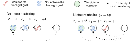
Figure 1: Diagram of $n$-step relabeling. Circles are states in a trajectory, and green circles refer to the states we evaluate. Suppose only the third state achieves the hindsight goal. One-step relabeling relabels only one transition and estimates return with the relabeled reward $r^{\prime}_{1}$. N-step relabeling relabels $n$ (taking $n=3$ for example) consecutive transitions and combines relabeled $n$-step rewards $\hat{r}_{1}=r^{\prime}_{1}+\gamma r^{\prime}_{2}+\gamma^{2}r^{\prime}_{3}$ to estimate the return, therefore it increases useful learning signals for training.

In this paper, we introduce a new framework, Multi-step Hindsight Experience Replay (MHER), which utilizes the correlation between transitions to obtain more positive samples than HER and improves sample efficiency greatly. The core technique of MHER is $n$-step relabeling (shown in Figure 1), which relabels $n$ consecutive transitions with achieved goals and computes relabeled $n$-step returns to estimate the value function. However, normally off-policy data in RL algorithms comes from earlier versions of the policy and is relatively on-policy, while the relabeled data in HER is completely off-policy (Plappert et al., 2018). Experimental results and theoretical analysis consistently show that vanilla MHER may perform inconsistently in different environments due to the off-policy $n$-step bias. This problem is considered to be a promising research topic by (Plappert et al., 2018) and further leads us to propose bias-reduced MHER algorithms.

To improve the sample efficiency of HER and tackle the above issue in vanilla MHER, we propose two algorithms, MHER($\lambda$) and Model-based MHER (MMHER). Inspired by TD($\lambda$) (Seijen and Sutton, 2014), MHER($\lambda$) combines relabeled $n$-step returns with exponentially decayed weights parameterized by $\lambda$, making a trade-off between bias and reward signals. Unlike MHER($\lambda$), MMHER alleviates off-policy bias by generating on-policy returns with a trained dynamics model. We conduct detailed experiments on eight challenging simulated robot environments (Plappert et al., 2018; Yu et al., 2020), including Sawyer, Fetch and Hand environments. Experimental results demonstrate that both of our two algorithms can alleviate off-policy $n$-step bias and outperform HER and Curriculum-guided HER (CHER) (Fang et al., 2019) in sample efficiency. To the best of our knowledge, our work is the first to successfully incorporate multi-step information to solve sparse-reward multi-goal RL problems.

In conclusion, our contributions can be summarized as follows:

• We present the framework of MHER based on $n$-step relabeling to incorporate multi-step relabeled rewards into HER;

• We analyze the off-policy $n$-step bias introduced by MHER theoretically and experimentally;

• We propose two simple but effective bias-reduced MHER algorithms, MHER($\lambda$) and MMHER, both of them successfully mitigate the off-policy $n$-step bias and achieve significantly higher sample efficiency than HER and CHER.

2 Related Work

In reinforcement learning, multi-step methods (Sutton, 1988; Watkins, 1989) have been studied for a long history since Monte Carlo (MC) and Temporal Difference (TD). Q($\lambda$)-learning (Peng and Williams, 1994) combines Q-learning and TD($\lambda$) for faster learning and alleviating the non-Markovian effect. Two well-known works, Rainbow (Hessel et al., 2018) and D4PG (Barth-Maron et al., 2018), utilize $n$-step returns to improve the performance of DQN (Mnih et al., 2015) and DDPG (Lillicrap et al., 2016). However, $n$-step returns in off-policy algorithms are biased due to policy mismatch. One bias-free solution is off-policy correction using Importance Sampling (IS) (Precup et al., 2000). Retrace($\lambda$) (Munos et al., 2016) is introduced to reduce the variance in IS with guaranteed efficiency. Overall, multi-step methods provide a forward view and contribute to a faster propagating of value estimation.

In contrast to multi-step methods, HER (Andrychowicz et al., 2017) provides a hindsight view in completed trajectories. Through hindsight relabeling with achieved goals, HER hugely boosts the sample efficiency in complex environments with sparse and binary rewards. A series of algorithms have been proposed to further improve the performance of HER. Energy-Based Prioritization (Zhao and Tresp, 2018) prioritizes experiences based on the trajectory energy for more efficient usage of collected data. Curriculum-guided HER (Fang et al., 2019) adaptively makes an exploration-exploitation trade-off to select hindsight goals. Maximum Entropy-based Prioritization (Zhao et al., 2019) introduces a weighted entropy to encourage agents to achieve more diverse goals. Concentrating on exploiting the information between transitions, our work is orthogonal to these algorithms.

In general, model-based RL algorithms have the advantage of higher sample efficiency over model-free algorithms (Nagabandi et al., 2018). Dyna (Sutton, 1991) utilizes a trained model to generate virtual transitions for accelerating learning value functions. However, model-based methods are limited by model bias, as previous work (Janner et al., 2019) addressed. Our model-based algorithm is closely related to Model-Based Value Expansion (MVE) (Feinberg et al., 2018), which applies model-based value expansion to enhance the estimation of expected returns. The differences are: 1) our model-based return is under the multi-goal setting, and 2) we utilize a compound form of MVE and hindsight relabeling to jointly exploit MVE and hindsight knowledge (see Section 6.2).

3 Preliminaries

3.1 Reinforcement Learning

Reinforcement learning (RL) solves the problem of how an agent acts to maximize cumulative rewards obtained from an environment. Generally, the RL problem is formalized as a Markov Decision Process (MDP), which consists of five elements, state space $\mathcal{S}$, action space $\mathcal{A}$, reward function $r:\mathcal{S}\times\mathcal{A}\rightarrow\mathbb{R}$, transition probability distribution $p(s^{\prime}|s,a)$, and discount factor $\gamma\in[0,1]$. The agent learns a policy $\pi:\mathcal{S}\rightarrow\mathcal{A}$ to maximize expected cumulative rewards $E[\sum_{t=0}^{\infty}\gamma^{t}r_{t}]$. The Q-function $Q:\mathcal{S}\times\mathcal{A}\rightarrow\mathbb{R}$ is defined as the expected return starting from the state-action pair $(s_{t},a_{t})$:

$$Q(s_{t},a_{t})=E\big{[}\sum_{k=0}^{\infty}\gamma^{k}r_{t+k}|s_{t},a_{t}\big{]}$$

3.2 Deep Deterministic Policy Gradient (DDPG)

DDPG (Lillicrap et al., 2016) is an off-policy algorithm for continuous control. An actor-critic structure is applied in DDPG, where the actor serves as the policy $\pi$ and the critic approximates the Q-function. Denote the replay buffer as $B$. The actor is updated with gradient descent on the loss:

$$L_{actor}=-E_{s_{t}\sim B}[Q(s_{t},\pi(s_{t}))].$$

The critic is updated to minimize the TD error:

$${L}_{critic}=E_{(s_{t},a_{t},s_{t+1})\sim B}[(y_{t}-Q(s_{t},a_{t}))^{2}],$$

where $y_{t}=r_{t}+\gamma Q(s_{t+1},\pi(s_{t+1}))$.

In D4PG (Barth-Maron et al., 2018), $n$-step returns are utilized to enhance the approximation of the value function, where $n$-step target $y^{(n)}_{t}$ is defined as:

$$y^{(n)}_{t}=\sum_{k=0}^{n-1}\gamma^{k}r_{t+k}+\gamma^{n}Q(s_{t+n},\pi(s_{t+n})).$$ (1)

3.3 Hindsight Experience Replay (HER)

HER (Andrychowicz et al., 2017) is proposed to tackle sparse reward problems in multi-goal RL. Following Universal Value Function Approximators (UVFA) (Schaul et al., 2015), HER considers goal-conditioned policy $\pi:\mathcal{S}\times\mathcal{G}\rightarrow\mathcal{A}$ and value function $Q:\mathcal{S}\times\mathcal{A}\times\mathcal{G}\rightarrow\mathbb{R}$. The sparse reward function is also conditioned by goals:

$$r(s_{t},a_{t},g)=\begin{cases}0,&\left|\left|\phi(s_{t})-g\right|\right|^{2}_{2}<\text{threshold}\cr-1,&\text{otherwise}\end{cases},$$ (2)

where $\phi:\mathcal{S}\rightarrow\mathcal{G}$ maps states to goals. The key technique of HER is hindsight relabeling, which relabels transition $(s_{t},a_{t},s_{t+1},r_{t},g)$ with achieved goal in the same trajectory $g^{\prime}=\phi(s_{t+k}),k\geq 0$ and new reward $r^{\prime}_{t}=r(s_{t},a_{t},g^{\prime})$ according to Eq. (2). After hindsight relabeling, HER augments training data with relabeled transitions $(s_{t},a_{t},r^{\prime}_{t},s_{t+1},g^{\prime})$ and increases the proportion of success trails, thereby alleviating the sparse reward problem and significantly improving sample efficiency.

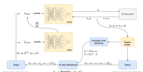
Figure 2: The Overall structure of MHER. Yellow modules are from DDPG, and blue modules belong to MHER. Major differences between HER and MHER are the blue modules in the bottom row. MHER selects $n$-step transitions using Select function and relabels these transitions using N-step Relabeling. After that we compute target with Target function to update the value function.

Initialize policy $\pi$ and value function $Q$ ;

for episode = $1,2,\ldots,M$ do

       Sample a desired goal $g$;

       Collect a $T$-step trajectory with $\pi$ and save to $B$;

       Sample a batch $b=\{(s_{t},a_{t},s_{t+1},r_{t},g)_{m}\}^{N}_{m=1}\sim B$;

       for $m=1,2,\ldots,N$ do

             $(s_{t},a_{t},s_{t+1},r_{t},g)\leftarrow b_{m}$ and set $g^{\prime}=g$;

             if $random()<\frac{k}{1+k}$ then

                   Sample future achieved goal $g^{\prime}$

             end if

            Select $n$ transitions using $Select(*args)$;

             Relabel $n$ transitions with $g^{\prime}$;

             Recompute each $r^{\prime}_{t+i}$ with $Reward(*args)$;

             Compute target $\hat{y}^{(n)}=Target(*args)$;

             $b_{m}\leftarrow(s_{t},a_{t},\hat{y}^{(n)},s_{t+1},g^{\prime})$

       end for

      Update $Q$ with $b$ by minimizing the loss:

       $\frac{1}{N}\Sigma(\hat{y}^{(n)}-Q(s_{t},a_{t},g^{\prime}))^{2}$
Update $\pi$ with $b$ according to $A$ ;

      

end for

Given: an off-policy RL algorithm $A$, a replay buffer $B$, a reward function $Reward$, the number of sample goals $k$, step number $n$, a target function $Target$, a selection function $Select$.

Algorithm 1 MHER Framework

Given: an off-policy RL algorithm $A$, a replay buffer $B$, a reward function $Reward$, the number of sample goals $k$, step number $n$, a target function $Target$, a selection function $Select$.

4 Multi-step Hindsight Experience Replay

In this section, we first introduce $n$-step relabeling and the MHER framework. Then we show a motivating example where vanilla MHER performs poorly. For demonstration purposes, all formulations are conducted in the DDPG+HER framework (Andrychowicz et al., 2017; Fang et al., 2019).

4.1 $N$-step Relabeling

In $n$-step relabeling, multiple transitions rather than just a single transition are relabeled, therefore more information between relabeled transitions can be exploited. Given $n$ consecutive transitions $\{(s_{t+i},a_{t+i},r_{t+i},s_{t+1+i},g)\}_{i=0}^{n-1}$ in a collected trajectory of length $T$, we alternate goals and rewards with $g^{\prime}=\phi(s_{t+k}),k\in[0,T-t]$ and $r^{\prime}_{t+i}=r(s_{t+i},a_{t+i},g^{\prime}),i\in[0,n-1]$, and then obtain relabeled transitions $\{(s_{t+i},a_{t+i},r^{\prime}_{t+i},s_{t+1+i},g^{\prime})\}_{i=0}^{n-1}$. After relabeling, we can compute relabeled $n$-step returns for value estimation:

$$y_{t}^{(n)}=\sum^{n-1}_{i=0}\gamma^{i}r^{\prime}_{t+i}+\gamma^{n}Q(s_{t+n},\pi(s_{t+n},g^{\prime}),g^{\prime}),$$ (3)

where goal $g^{\prime}$ is included in action-value function $Q$ and policy $\pi$ following UVFA (Schaul et al., 2015).

Consider a situation where only one state in the trajectory achieves the hindsight goal, as shown in Figure 1. One-step relabeling only holds a single non-negative sample for this trajectory while $n$-step relabeling possesses $n$ non-negative samples. Therefore, $n$-step relabeling remarkably contributes to solving sparse reward problems, for which non-negative learning signals are very crucial.

4.2 MHER Framework

The overall framework of MHER is presented in Algorithm 1 and Figure 2. After collecting a $T$-step trajectory into the replay buffer, we randomly sample a minibatch $b$ from the buffer. For every transition in $b$ we sample a future goal $g^{\prime}$ according to a certain probability $\frac{k}{1+k}$, where $k$ represents the ratio of the relabeled data to the original data. Next, for each transition we select $n$ consecutive transitions with the $Select$ function. Then, we perform $n$-step relabeling and compute relabeled $n$-step target $\hat{y}^{(n)}$ using the $Target$ function. Finally, the Q-function is updated with target $\hat{y}^{(n)}$ and the policy is trained by any off-policy RL algorithm such as DDPG and SAC (Haarnoja et al., 2018). For vanilla MHER, the $Target$ function is Eq.(3) and the $Select$ function outputs $n$ consecutive transitions in the same trajectory: $\{(s_{t+i},a_{t+i},r_{t+i},s_{t+1+i},g)\}_{i=0}^{n-1},n=min\{n,T-t\}$.

[] []

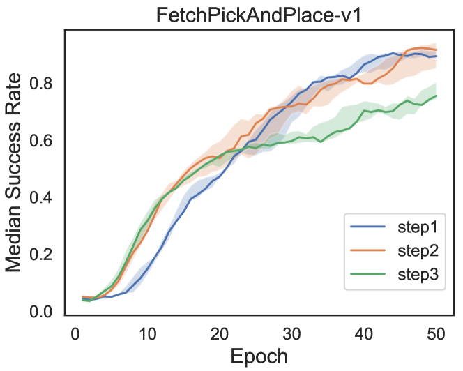
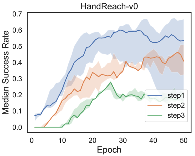
Figure 3: Performance of vanilla MHER in simulated robotics environments. There is a clear performance decreases when steps increase.

4.3 A Motivating Example of Bias-reduced MHER

We compare vanilla MHER with HER ($n=1$) in simulated robotics environments and results are shown in Figure 3. There is a clear performance decrease when $n$ is large in both Fetch and Hand environments. In addition, the performance decrease in HandReach is more significant than that in FetchPickAndPlace. The primary reason behind this is the off-policy $n$-step bias, which we will discuss in the following section.

5 Off-policy $N$-step Bias

The relabeled $n$-step returns in MHER introduce bias due to the discrepancy of the data collecting policy and the target policy. Such bias is the main reason for MHER’s poor performance in Figure 3. In this section, we study the off-policy $n$-step bias through theoretical and empirical analysis. For brevity, we omit goals $g$ as it can be included as part of states.

Proposition 5.1.

Given $n$-step transitions under data collecting policy $\mu$: $\{(s_{t},a_{t},r_{t},s_{t+1})\}_{t=0}^{n-1}$, target policy $\pi$, discount factor $\gamma$, action value function $Q$. Policies $\mu$ and $\pi$ are deterministic. The off-policy $n$-step bias $\mathcal{B}_{t}^{(n)}$ at time step $t$ has the following formula:

$$\mathcal{B}_{t}^{(n)}=\sum_{i=1}^{n-1}\gamma^{i}[Q(s_{t+i},\pi(s_{t+i}))-Q(s_{t+i},a_{t+i})].$$ (4)

The proof is provided in Appendix A in the supplementary file. Although the sign of the $i$-th term in Eq. (4) is uncertain, each term has a higher probability of being non-negative as the policy $\pi$ is learned to maximize $E[Q(s,\pi(s))]$. For further analysis, we define the average off-policy $n$-step bias and the absolute average reward in the replay buffer as:

$$\mathcal{B}^{(n)}=E_{(s_{t+i},a_{t+i},s_{t+i+1})_{i=0}^{n-1}\sim B}\big{[}\mathcal{B}_{t}^{(n)}\big{]}$$ (5)

$$\bar{r}_{abs}=|E_{r_{t}\sim B}[r_{t}]|$$ (6)

where $B$ refers to the replay buffer, and $\bar{r}_{abs}$ reflects the difficulty of the task to a certain extent when using the sparse reward function.

5.1 Intuitive Analysis of $\mathcal{B}^{(n)}$

From Eq. (4) and Eq. (5), we can conclude that there are three key factors affecting $\mathcal{B}^{(n)}$, step number $n$, policy $\pi$, and value function $Q$:

• $\mathcal{B}^{(n)}$ equals zero when $n=1$ and accumulates as $n$ increases;

• $\mathcal{B}^{(n)}$ equals zero when $\pi=\mu$ ($\mu$ is the data collecting policy), otherwise accumulates as the shift of $\pi$ and $\mu$ increases;

• $\mathcal{B}^{(n)}$ increases as the magnitude of the gradient of $Q$ (related to average reward) increases.

Note that in MHER setting, the data collecting policy $\mu$ is the policy generating the relabeled data and differs from early versions of the agent’s policy (Plappert et al., 2018). Therefore, the second factor is more difficult to control than previous works (Hessel et al., 2018; Barth-Maron et al., 2018). In Proposition 5.2, we give an upper bound on $\mathcal{B}^{(n)}$ to show the connection between $\mathcal{B}^{(n)}$ and the absolute average reward $\bar{r}_{abs}$ in Eq. (6).

Proposition 5.2.

Denote action value function under current policy $Q(s,\pi(s))$ as $V^{\pi}(s)$. The reward function is defined in Eq. (2). Assuming $V^{\pi}(s)$ is Lipschitz continuous with constant $L$ for $\forall s,s^{\prime}\in S$, the average off-policy $n$-step bias can be bounded as follows:

$$\mathcal{B}^{(n)}\leq\gamma(n-1)\big{[}|E_{r_{t}\sim B}[r_{t}]|+\gamma LE_{(s_{t},s_{t+1})\sim B}\|s_{t}-s_{t+1}\|\big{]}$$ (7)

The proof and the tightness analysis of the bound are in Appendix B. Proposition 5.2 evidently indicates that the absolute average reward has an impact on the average off-policy $n$-step bias $B^{(n)}$. Furthermore, $B^{(n)}$ is environment-specific as the absolute average reward varies with different environmental difficulties, i.e., tasks with larger absolute average reward may obtain larger off-policy $n$-step bias.

5.2 Empirical Analysis of $\mathcal{B}^{(n)}$

The above analysis is experimentally verified. Average off-policy $n$-step bias computed by Eq. (4) and average reward using HER are plotted in Figure 4 (a) and Figure 4 (b), respectively. In Figure 4 (a), the bias of $3$-step MHER in the same environment is usually larger than $2$-step. Meanwhile, larger absolute average reward in HandReach (see Figure 4 (b)) leads to larger bias than FetchSlide. It needs to be emphasized that the bias in Figure 4 (a) is estimated using the learned value function rather than the true value function.

[] []

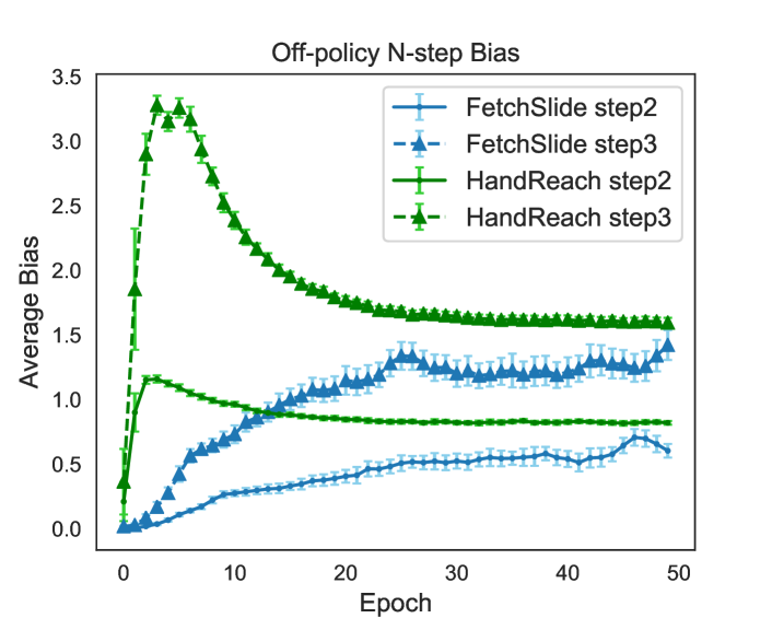
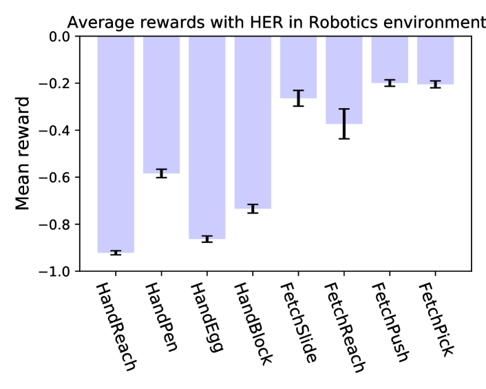
Figure 4: (a) Off-policy $n$-step bias training with vanilla MHER in FetchSlide and HandReach environments. (b) Average rewards training using HER in Robotics environments. The rewards are recorded during training HER for $50$ epochs.

function Select-MHER($\lambda$)($*args$):

       Get trajectory $\mathcal{T}$ and the transition index $t$

       Set $n=min(n,length(\mathcal{T})-t)$

      

return $\{(s_{t+i},a_{t+i},r_{t+i},s_{t+1+i},g_{t+i})\}_{i=0}^{n-1}$

function Target-MHER($\lambda$)($*args$):

       for $i=1,\ldots,n$ do

             Compute $y_{t}^{(i)}$ using Eq. (3)

            

       end for

      $\hat{y}^{(n)}=\frac{\Sigma_{i=1}^{n}\lambda^{i}\cdot y_{t}^{(i)}}{\Sigma_{i=1}^{n}\lambda^{i}}$ according to Eq. (8)

      

return $\hat{y}^{(n)}$

function Select-MMHER($*args$):

       Get $(s_{t},a_{t},r_{t},s_{t+1},g^{\prime})$ from $*args$

       $b=\{(s_{t},a_{t},r_{t},s_{t+1},g^{\prime})\}$

       for $i=1,\ldots,n-1$ do

             $a_{t+i}=\pi(s_{t+i},g^{\prime})$

             $s_{t+i+1}=model(s_{t+i},a_{t+i})$

             $r_{t+i}=reward(s_{t+i+1},g^{\prime})$

             Add $(s_{t+i},a_{t+i},r_{t+i},s_{t+i+1},g^{\prime})$ to $b$

            

       end for

      

return $b$

function Target-MMHER($*args$):

       Compute $y_{t}^{(n)}$ according to Eq. (9)

       Compute $\hat{y}^{(n)}$ according to Eq. (10)

      

return $\hat{y}^{(n)}$

Algorithm 2 Functions of Proposed Methods

6 Bias-reduced MHER Algorithms

In this section, we present two algorithms to reduce the off-policy $n$-step bias in MHER with the idea of $\lambda$ return (Seijen and Sutton, 2014) and model-based $n$-step value expansion (Feinberg et al., 2018). All the functions of proposed methods are shown in Algorithm 2.

6.1 MHER($\lambda$)

Inspired by TD($\lambda$) where a bias-variance trade-off is made between TD($0$) and MC, we propose MHER($\lambda$) to balance between lower bias as one-step target and more reward information as $n$-step target. An exponential decay weight parameter $\lambda\in[0,1]$ is introduced to combine $n$-step targets $y_{t}^{(i)},i\in[1,n]$ computed by Eq. (3):

$$\hat{y}^{(n)}=\frac{\sum_{i=1}^{n}\lambda^{i}y_{t}^{(i)}}{\sum_{i=1}^{n}\lambda^{i}}.$$ (8)

For an intuitive analysis on Eq. (8), $\hat{y}^{(n)}$ becomes close to $1$-step target without bias if $\lambda\rightarrow 0$ and assigns more weight on $n$-step target as $\lambda$ increases. Therefore, $\lambda$ makes a trade-off between bias and reward information provided by off-policy $n$-step returns. By adjusting the parameter $\lambda$, MHER($\lambda$) can adapt to different environments regardless of environmental difficulties and absolute average rewards.

6.2 Model-based MHER(MMHER)

MMHER generates on-policy value expansion with current policy and a learned dynamics model to alleviate the off-policy bias. As discussed in Section 5.1, on-policy returns don’t contain off-policy bias. In MMHER, a model $m:\mathcal{S}\times\mathcal{A}\rightarrow\mathcal{S}$ is trained to fit environmental dynamics by minimizing the following loss:

$$\mathcal{L}_{dynamics}=E_{(s_{t},a_{t},s_{t+1})\sim B}\|s_{t+1}-m(s_{t},a_{t})\|_{2}^{2},$$

where $B$ refers to the replay buffer. Details of training the dynamics model $m$ are presented in Appendix LABEL:detailMMHER.

Fully on-policy experiences cannot benefit from hindsight relabeling, thus we start model-based interaction with the relabeled goal $g^{\prime}$. Specifically, given a transition in the replay buffer $(s_{t},a_{t},r_{t},s_{t+1},g)$, we relabel it with $g^{\prime}$ and $r_{t}^{\prime}$ according to Section 3.3. Then we start from $s_{t+1}$ and use the trained model $m$ and current policy $\pi$ to generate $n-1$ transitions $(s^{\prime}_{t+i},a^{\prime}_{t+i},r^{\prime}_{t+i},s^{\prime}_{t+i+1},g^{\prime}),i\in[1,n-1],s^{\prime}_{t+1}=s_{t+1}$. Finally, we expand the target to $n$-step as:

$$y_{t}^{(n)}=\sum_{i=0}^{n-1}\gamma^{i}r^{\prime}_{t+i}+\gamma^{n}Q(s^{\prime}_{t+n},\pi(s^{\prime}_{t+n},g^{\prime}),g^{\prime}),$$ (9)

where $r^{\prime}_{t}$ can directly benefit from hindsight relabeling. With the relabeled goal $g^{\prime}$, the expanded target also contributes to the value estimation in sparse reward setting. If the model is accurate, $y_{t}^{(n)}$ is an unbiased $n$-step estimation of $Q(s_{t},a_{t},g^{\prime})$.

However, model-based methods encounter with model bias caused by the difference between the trained model and real environment (Janner et al., 2019), especially when the environment has high-dimensional states and complex dynamics. To balance between model bias and learning information, we utilize a weighted average of $n$-step target and one-step target using a parameter $\alpha$:

$$\hat{y}^{(n)}=\frac{\alpha\times y_{t}^{(n)}+(r^{\prime}_{t}+\gamma Q(s_{t+1},\pi(s_{t+1},g^{\prime}),g^{\prime}))}{\alpha+1}.$$ (10)

When $\alpha\rightarrow 0$, $\hat{y}^{(n)}$ is close to unbiased $1$-step return. As $\alpha$ increases, $\hat{y}^{(n)}$ gains more information from model-based $n$-step returns but meanwhile contains more model bias.

[] [] [] []

[] [] [] []

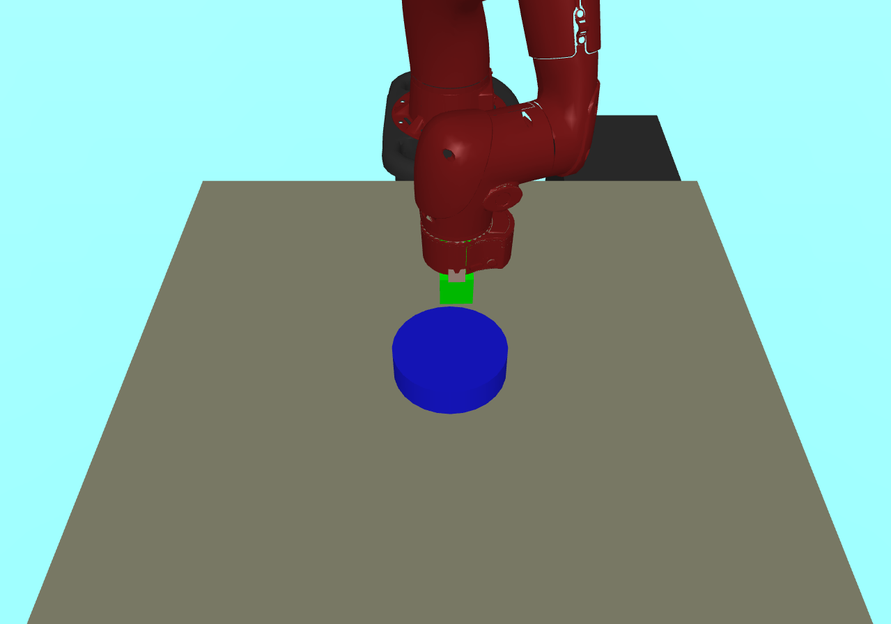
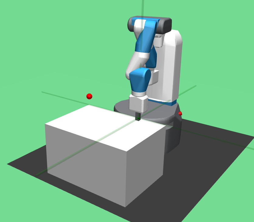
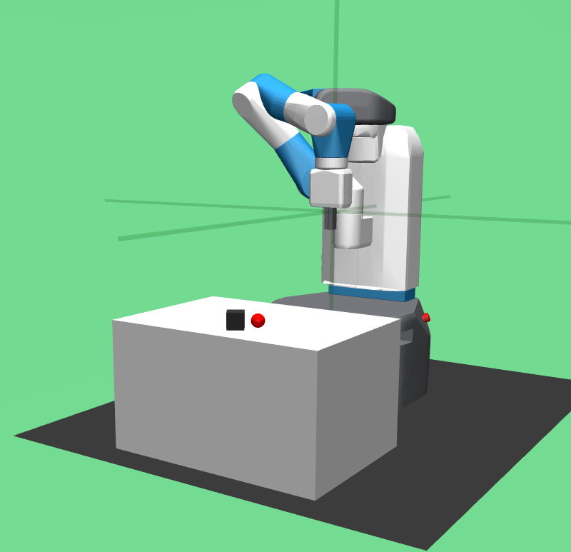
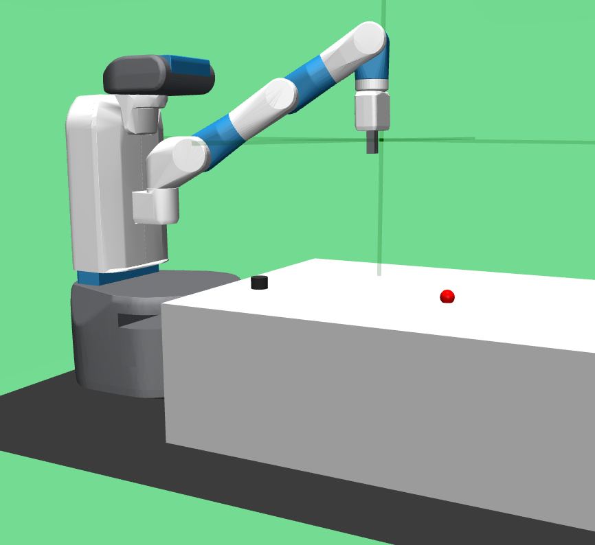
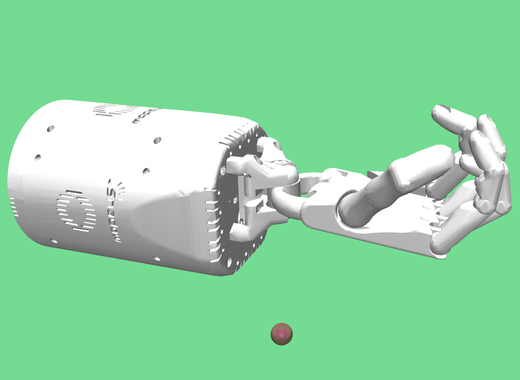
Figure 5: Eight simulated robotics environments: (a) SawyerReachXYZEnv-v1, (b) SawyerPushAndReachEnvEasy-v0, (c) FetchReach-v1, (d) FetchPush-v1, (e) FetchSlide-v1, (f) FetchPickAndPlace-v1, (g) HandReach-v0, (h) HandManipulateBlockRotateXYZ-v0.

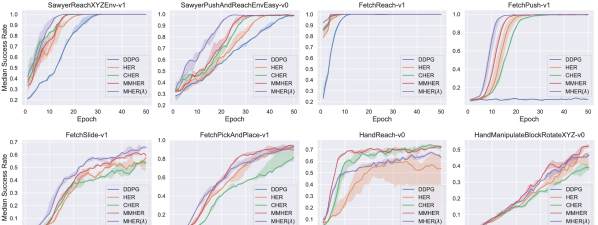
Figure 6: Median test success rate (line) with interquartile range (shaded area) in robotics environments.

7 Experiments

We evaluate MHER($\lambda$) and MMHER in eight challenging multi-goal robotics environments and compare them to three baselines: DDPG, original HER, and CHER (Fang et al., 2019). For each experiment, we train for 50 epochs with 12 parallel environments and a central learner, which has the advantage of better utilization of GPU. We sample 12 trajectories in every cycle and train all the algorithms for 40 batches. Three relatively easy tasks (SawyerReach, SawyerPush, and FetchReach), contain 10 cycles each epoch, while other tasks contain 50 cycles each epoch. In order to emphasize the sample efficiency, we only sample $12\times 50$ trajectories ($12\times 10$ for the three easy tasks) each epoch and train the central learner with a batch size of $1024$, which is approximately $1/3$ of samples and $1/5$ of the computation in previous work (Plappert et al., 2018). Detailed hyperparameters are listed in Appendix LABEL:ap:hyperpara.

In benchmark experiments, we select $n=3,\lambda=0.7$ for MHER($\lambda$) in Sawyer and Fetch environments, and $n=2,\lambda=0.7$ in Hand environments. As for MMHER, the parameter $\alpha$ and step number $n$ are set to $0.4$ and $2$ respectively across all environments.

After training for one epoch, we test without action noise for 120 episodes to accurately evaluate the performance of algorithms. For all the experiments, we repeat experiments using $5$ random seeds and depict the median test success rate with the interquartile range.

7.1 Environments

As shown in Figure 5, eight challenging robotics environments are included in our experiments. In each environment, agents are required either to reach the desired state or manipulate a specific object to the target pose. Agents receive a reward of $0$ if successfully achieve the desired goal, and a reward of $-1$ otherwise. The Sawyer, Fetch and Hand environments are taken from (Yu et al., 2020) and (Plappert et al., 2018) respectively. A more detailed introduction of environments is as follows.

7.1.1 Sawyer Environments

The Sawyer robot’s observations are $3$-dimensional vectors representing the 3D Cartesian positions of the end-effector. Similarly, goals are $3$-dimensional vectors describing the position of the target place. The action space is also $3$-dimensional which indicates the next expected position of the end-effector.

7.1.2 Fetch Environments

The robot in Fetch environments is a 7-DoF robotic arm with a two-finger gripper and it aims to touch the desired position or push, slide, place an object to the target place. Observations contain the gripper’s position and linear velocities (10 dimensions). If the object exists, another 15 dimensions about its position, rotation, and velocities are also included. Actions are 4-dimensional vectors representing grippers’ movements and their opening and closing. Goals are 3-dimensional vectors describing the expected positions of the gripper or the object.

7.1.3 Hand Environments

Hand environments are constructed with a $24$-DoF anthropomorphic robotic hand and aim to control its fingers to reach the target place or manipulate a specific object (e.g., a block) to the desired position. Observations contain two $24$-dimensional vectors about positions and velocities of the joints. Additional $7$ or $15$ dimensions indicating current state of the object or fingertips are also included. Actions are 20-dimensional vectors and control the non-coupled joints of the hand. Goals have $15$ dimensions for HandReach containing the target Cartesian position of each fingertip or $7$ dimensions for HandBlock representing the object’s desired position and rotation.

[] []

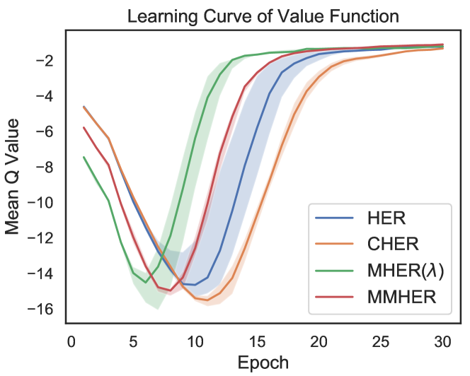
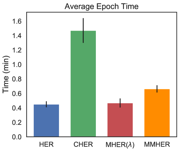
Figure 7: (a) Learning curves of Q value using different algorithms in FetchPush environment, (b) average epoch time of different algorithms in SawyerPushAndReachEnvEasy environment.

7.2 Benchmark Results

Figure 6 reports the performance of five algorithms in eight environments. The experimental results clearly show that our methods can achieve faster training speed and higher average success rate compared with HER and CHER, even in Hand environments where off-policy $n$-step bias is quite large. Comparing with the results in figure 3, MHER($\lambda$) and MMHER successfully alleviate the impact of off-policy bias in vanilla MHER and bring considerable performance improvement.

Furthermore, we depict the learning curves of Q-function and the average epoch time in Figure 7. Figure 7 (a) implies that MHER($\lambda$) and MMHER contribute to fast learning of value functions compared to HER and CHER. On average, the learned value function does not deviate from the convergent value of HER. Figure 7 (b) provides evidence that our two algorithms also have computational advantages over CHER. The results also demonstrate that MHER($\lambda$) improves performance significantly at less cost of computation resources than CHER and MMHER.

7.3 MHER($\lambda$) vs MMHER

In Figure 6, the results demonstrate that MHER($\lambda$) performs better than MMHER in most Sawyer and Fetch environments while MMHER performs better in Hand environments. Considering the difference of average rewards discussed in Figure 4 and Section 5, we can conclude that MHER($\lambda$) is more considerable when handling tasks with relatively smaller absolute average rewards. On the contrary, when in environments with large absolute average rewards where off-policy $n$-step bias is aggravated, MMHER is more favorable as it utilizes model-based on-policy returns and is less affected by the off-policy bias.

[] []

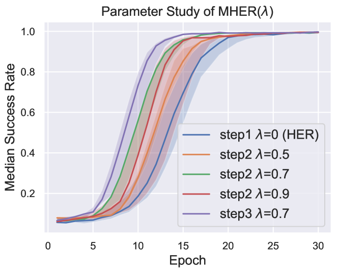
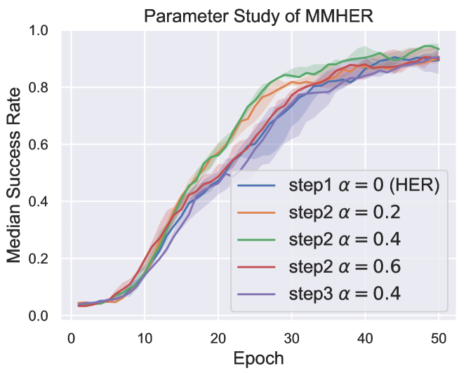
Figure 8: (a) Parameter study for MHER($\lambda$) in FetchPush, (b) parameter study for MMHER in FetchPickAndPlace.

7.4 Parameter Study

We then take an insight into how different parameters affect the performance of MHER($\lambda$) and MMHER. Comparison results in FetchPush and FetchPickAndPlace environments are shown in Figure 8. From Figure 8 (a) we can conclude that $\lambda=0.7$ successfully makes a trade-off between bias and learning speed, i.e., bigger $\lambda$ suffers from off-policy bias and smaller $\lambda$ learns slowly. Moreover, $3$-step MHER($\lambda$) outperforms $2$-step in FetchPush environment. As for MMHER in Figure 8 (b), there is also an apparent trade-off between model bias and learning speed with different $\alpha$. The result of $\alpha=0.4$ is the best in $\{0.2,0.4,0.6\}$. Besides, 3-step MMHER performs relatively worse than 2-step, which is mainly because the model bias accumulates as the step number $n$ increases.

8 Conclusion

Based on our idea of Multi-step Hindsight Experience Replay and analysis about the off-policy $n$-step bias, we propose two effective algorithms, MHER($\lambda$) and MMHER, both of which successfully mitigate the off-policy $n$-step bias and improve sample efficiency in sparse-reward multi-goal tasks. The two algorithms alleviate the off-policy $n$-step bias with an exponentially decreasing weighted sum of $n$-step targets and model-based value expansion, respectively. Experiments conducted in eight challenging robotics environments demonstrate that our two algorithms outperform HER and CHER significantly in sample efficiency at the cost of little additional computation beyond HER. Further analysis of experimental results suggests MHER($\lambda$) is more suitable for environments with small absolute average rewards, while MMHER is more favorable in environments with large absolute average rewards where off-policy $n$-step bias is aggravated.

Appendix A Proof of Proposition 1

Proof A.1.

For deterministic policy, action-value function $Q(s_{t},a_{t})$ has the following unbiased estimation:

$$\begin{split}Q(s_{t},a_{t})&=\mathbb{E}_{r_{t}\sim r(s_{t},a_{t}),s_{t+1}\sim p(\cdot|s_{t},a_{t})}\big{[}r_{t}+\gamma\mathbb{E}_{\pi}[Q(s_{t+1},\cdot)]\big{]}\\ &=\mathbb{E}_{r_{t}\sim r(s_{t},a_{t}),s_{t+1}\sim p(\cdot|s_{t},a_{t})}\big{[}r_{t}+\gamma Q(s_{t+1},\pi(s_{t+1}))\big{]},\end{split}$$

where $p$ refers to the state transition probability and $r$ refers to reward function. The following equations also hold by recursion:

$$Q(s_{t},a_{t}) =\mathbb{E}[r_{t}+\gamma Q(s_{t+1},\pi(s_{t+1}))]$$ (11)

$$=\mathbb{E}[r_{t}+\gamma Q(s_{t+1},a_{t+1})+\gamma Q(s_{t+1},\pi(s_{t+1}))-\gamma Q(s_{t+1},a_{t+1})]$$

$$=\mathbb{E}[r_{t}+\gamma\mathbb{E}[r_{t+1}+\gamma Q(s_{t+2},\pi(s_{t+2}))]+\gamma(Q(s_{t+1},\pi(s_{t+1}))-Q(s_{t+1},a_{t+1}))]$$

$$=\ldots$$

$$=\mathbb{E}\Bigg{[}\sum_{i=0}^{n-1}\gamma^{i}r_{t+i}+\gamma^{n}Q(s_{t+n},\pi(s_{t+n}))+\sum_{i=1}^{n-1}\gamma^{i}\big{[}Q(s_{t+i},\pi(s_{t+i}))-Q(s_{t+i},a_{t+i})\big{]}\Bigg{]}.$$

Eq. (11) gives an unbiased estimation of $Q(S_{t},a_{t})$. Comparing Eq. (11) to the $n$-step target in Eq. (1), we conclude that off-policy $n$-step bias $\mathcal{B}_{t}^{(n)}$ at time $t$ has the following formula:

$$\mathcal{B}_{t}^{(n)}=\sum_{i=1}^{n-1}\gamma^{i}[Q(s_{t+i},\pi(s_{t+i}))-Q(s_{t+i},a_{t+i})].$$

Appendix B Proof of Proposition 2

References

- Andrychowicz et al. (2017) Marcin Andrychowicz, Filip Wolski, Alex Ray, Jonas Schneider, Rachel Fong, Peter Welinder, Bob McGrew, Josh Tobin, OpenAI Pieter Abbeel, and Wojciech Zaremba. Hindsight experience replay. In Advances in Neural Information Processing Systems, pages 5048–5058, 2017.
- Barth-Maron et al. (2018) Gabriel Barth-Maron, Matthew W Hoffman, David Budden, Will Dabney, Dan Horgan, TB Dhruva, Alistair Muldal, Nicolas Heess, and Timothy Lillicrap. Distributed distributional deterministic policy gradients. In International Conference on Learning Representations, 2018.
- D’Eramo et al. (2019) Carlo D’Eramo, Davide Tateo, Andrea Bonarini, Marcello Restelli, and Jan Peters. Sharing knowledge in multi-task deep reinforcement learning. In International Conference on Learning Representations, 2019.
- Fang et al. (2019) Meng Fang, Tianyi Zhou, Yali Du, Lei Han, and Zhengyou Zhang. Curriculum-guided hindsight experience replay. In Advances in Neural Information Processing Systems, pages 12623–12634, 2019.
- Feinberg et al. (2018) Vladimir Feinberg, Alvin Wan, Ion Stoica, Michael I Jordan, Joseph E Gonzalez, and Sergey Levine. Model-based value estimation for efficient model-free reinforcement learning. arXiv preprint arXiv:1803.00101, 2018.
- Haarnoja et al. (2018) Tuomas Haarnoja, Aurick Zhou, Pieter Abbeel, and Sergey Levine. Soft actor-critic: Off-policy maximum entropy deep reinforcement learning with a stochastic actor. In International Conference on Machine Learning, pages 1861–1870, 2018.
- Hessel et al. (2018) Matteo Hessel, Joseph Modayil, Hado van Hasselt, Tom Schaul, Georg Ostrovski, Will Dabney, Dan Horgan, Bilal Piot, Mohammad Gheshlaghi Azar, and David Silver. Rainbow: Combining improvements in deep reinforcement learning. In AAAI Conference on Artificial Intelligence, 2018.
- Janner et al. (2019) Michael Janner, Justin Fu, Marvin Zhang, and Sergey Levine. When to trust your model: Model-based policy optimization. In Advances in Neural Information Processing Systems, pages 12519–12530, 2019.
- Kim and Park (2009) Dongsun Kim and Sooyong Park. Reinforcement learning-based dynamic adaptation planning method for architecture-based self-managed software. In 2009 ICSE Workshop on Software Engineering for Adaptive and Self-Managing Systems, pages 76–85. IEEE, 2009.
- Kober et al. (2013) Jens Kober, J Andrew Bagnell, and Jan Peters. Reinforcement learning in robotics: A survey. The International Journal of Robotics Research, 32(11):1238–1274, 2013.
- Lillicrap et al. (2016) Timothy P Lillicrap, Jonathan J Hunt, Alexander Pritzel, Nicolas Heess, Tom Erez, Yuval Tassa, David Silver, and Daan Wierstra. Continuous control with deep reinforcement learning. In International Conference on Learning Representations, 2016.
- Mnih et al. (2015) Volodymyr Mnih, Koray Kavukcuoglu, David Silver, Andrei A Rusu, Joel Veness, Marc G Bellemare, Alex Graves, Martin Riedmiller, Andreas K Fidjeland, Georg Ostrovski, et al. Human-level control through deep reinforcement learning. Nature, 518(7540):529–533, 2015.
- Munos et al. (2016) Rémi Munos, Tom Stepleton, Anna Harutyunyan, and Marc Bellemare. Safe and efficient off-policy reinforcement learning. In Advances in Neural Information Processing Systems, pages 1054–1062, 2016.
- Nagabandi et al. (2018) Anusha Nagabandi, Gregory Kahn, Ronald S Fearing, and Sergey Levine. Neural network dynamics for model-based deep reinforcement learning with model-free fine-tuning. In 2018 IEEE International Conference on Robotics and Automation, pages 7559–7566, 2018.
- Ng et al. (1999) Andrew Y Ng, Daishi Harada, and Stuart Russell. Policy invariance under reward transformations: Theory and application to reward shaping. In International Conference on Machine Learning, volume 99, pages 278–287, 1999.
- Peng and Williams (1994) Jing Peng and Ronald J Williams. Incremental multi-step q-learning. In Machine Learning Proceedings 1994, pages 226–232. Elsevier, 1994.
- Plappert et al. (2018) Matthias Plappert, Marcin Andrychowicz, Alex Ray, Bob McGrew, Bowen Baker, Glenn Powell, Jonas Schneider, Josh Tobin, Maciek Chociej, Peter Welinder, et al. Multi-goal reinforcement learning: Challenging robotics environments and request for research. arXiv preprint arXiv:1802.09464, 2018.
- Precup et al. (2000) Doina Precup, Richard S Sutton, and Satinder Singh. Eligibility traces for off-policy policy evaluation. In International Conference on Machine Learning, pages 759–766, 2000.
- Schaul et al. (2015) Tom Schaul, Daniel Horgan, Karol Gregor, and David Silver. Universal value function approximators. In International Conference on Machine Learning, pages 1312–1320, 2015.
- Seijen and Sutton (2014) Harm Seijen and Rich Sutton. True online td (lambda). In International Conference on Machine Learning, pages 692–700, 2014.
- Sutton (1988) Richard S Sutton. Learning to predict by the methods of temporal differences. Machine learning, 3(1):9–44, 1988.
- Sutton (1991) Richard S Sutton. Dyna, an integrated architecture for learning, planning, and reacting. ACM Sigart Bulletin, 2(4):160–163, 1991.
- Watkins (1989) Christopher John Cornish Hellaby Watkins. Learning from delayed rewards. 1989.
- Yu et al. (2020) Tianhe Yu, Deirdre Quillen, Zhanpeng He, Ryan Julian, Karol Hausman, Chelsea Finn, and Sergey Levine. Meta-world: A benchmark and evaluation for multi-task and meta reinforcement learning. In Conference on Robot Learning, pages 1094–1100, 2020.
- Zhang et al. (2015) Fangyi Zhang, Juergen Leitner, Michael Milford, Ben Upcroft, and Peter Corke. Towards vision-based deep reinforcement learning for robotic motion control. In Proceedings of the Australasian Conference on Robotics and Automation 2015:, pages 1–8. Australian Robotics and Automation Association, 2015.
- Zhao and Tresp (2018) Rui Zhao and Volker Tresp. Energy-based hindsight experience prioritization. In Conference on Robot Learning, pages 113–122, 2018.
- Zhao et al. (2019) Rui Zhao, Xudong Sun, and Volker Tresp. Maximum entropy-regularized multi-goal reinforcement learning. In International Conference on Machine Learning, pages 7553–7562, 2019.