Evolving Attention with Residual Convolutions
Abstract
Transformer is a ubiquitous model for natural language processing and has attracted wide attentions in computer vision. The attention maps are indispensable for a transformer model to encode the dependencies among input tokens. However, they are learned independently in each layer and sometimes fail to capture precise patterns. In this paper, we propose a novel and generic mechanism based on evolving attention to improve the performance of transformers. On one hand, the attention maps in different layers share common knowledge, thus the ones in preceding layers can instruct the attention in succeeding layers through residual connections. On the other hand, low-level and high-level attentions vary in the level of abstraction, so we adopt convolutional layers to model the evolutionary process of attention maps. The proposed evolving attention mechanism achieves significant performance improvement over various state-of-the-art models for multiple tasks, including image classification, natural language understanding and machine translation.
1 Introduction
Transformer (Vaswani et al., 2017) is the state-of-the-art architecture for sequential modeling which achieves superior performances in various applications, such as natural language understanding (Devlin et al., 2019), image generation (Parmar et al., 2018) and time-series forecasting (Li et al., 2019). The performance of a transformer model mainly depends on its capability of inducing reasonable attentions between input tokens. However, as illustrated by some previous works (Tang et al., 2018; Jain & Wallace, 2019), the attention maps captured by vanilla attention layers are not always effective and explainable. To cope with this problem, recent efforts concatenated self-attentions with convolutional layers to obtain better image or text representations (Bello et al., 2019; Wu et al., 2020), whereas the attention map itself was not ameliorated. In this paper, we consider another question, can we improve the learning of attention maps via a dedicated model architecture design? As we will illustrate, it is possible to improve the quality of attention maps by an evolving mechanism based on a chain of convolutional modules.
In a vanilla transformer, the attention maps in each layer are learned independently, which do not have good generalization ability. Intuitively, one can simply share attention maps among layers, but it is not effective as different layers may require attention structures from different abstraction levels. For instance, in image classification, a lower layer usually focuses on the relations within similar colors and textures, while a higher layer needs to reason about dependencies between components. Our motivation is to design a dedicated module to improve the quality of attention maps in an evolutionary process. Therefore, we directly bridge the attention maps from different layers through residual connections. Moreover, we adopt convolutional layers to capture the evolution of attention patterns, as this inductive bias emphasizes local details and produces more precise attention maps by reasoning on previous ones.
To this end, we propose Evolving Attention (EA-) Transformer, which guides the learning of attention maps via a chain of residual convolutional modules coupled with the transformer architecture. In each block, EA-Transformer takes all attention maps generated by the previous block as a multi-channel image. Then, with 2D-convolution over that image, the attention maps for the current block can evolve from previous ones efficiently. As such, the generic patterns of inter-token dependencies are shared across all blocks, and the attention maps are adapted to an appropriate abstraction level for each layer.
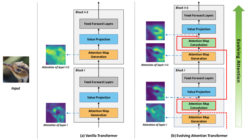
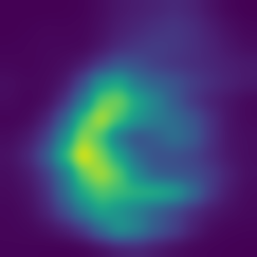
As illustrated by a case of ImageNet classification in Figure 2, the attention maps learned by EA-Transformer correctly highlight the structure of a bird with the help of convolution-based attention evolution. Especially, the residual links between attention maps facilitate the information flow of inter-token relations. Meanwhile, the convolutional module imitates an evolutionary mechanism and guides the self-attention layer to induce better attention maps. In contrast, the vanilla transformer learns each layer separately and sometimes produces vague attention structures.
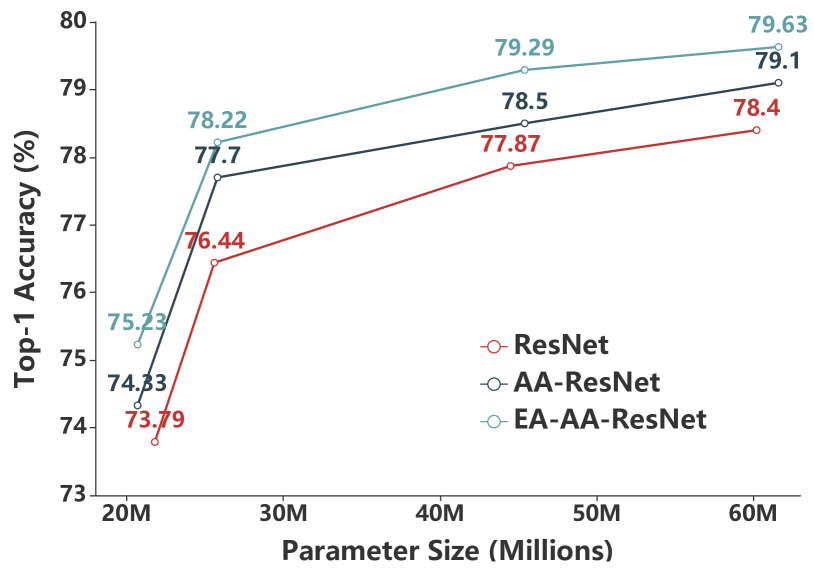
We apply the generic idea of evolving attention to multiple state-of-the-art models, including Transformer (Vaswani et al., 2017), BERT (Devlin et al., 2019) and Attention Augmented (AA-) ResNet (Bello et al., 2019). Experimental results demonstrate the superiority of evolving attention for various tasks in computer vision and natural language processing domains. As shown in Figure 1, for ImageNet classification, it consistently improves the accuracy of AA-ResNet with different model capacities. AA-ResNet is a strong SOTA which encapsulates self-attentions and convolutions jointly for image representation. We also examine the generality of evolving attention in BERT-style pre-trained models. Impressively, the average GLUE scores are lifted by 2.4, 1.1, 1.6 and 0.8 points from BERT-Base, T5-Base, BERT-Large, and RoBERTa-Large respectively.
The contributions of this paper are highlighted as follows.
-
•
We propose a novel evolving attention mechanism augmented by a chain of residual convolutional modules. To the best of our knowledge, this is the first work that considers attention maps as multi-channel images for pattern extraction and evolution, which sheds new lights on the attention mechanism.
-
•
Extensive experiments have demonstrated consistent improvement in various natural language and computer vision tasks. As indicated by extensive analysis, both residual connections and convolutional inductive bias are beneficial to produce better attention maps.
-
•
The proposed evolving attention mechanism is generally applicable for attention-based architectures and has further impacts on a broader range of applications.
2 Related Work
Transformer is first introduced by Vaswani et al. (2017) for machine translation and then widely adopted in numerous tasks in natural language (Devlin et al., 2019), computer vision (Parmar et al., 2018, 2019) and time-series (Li et al., 2019) domains. Transformer is solely composed of self-attention and feed-forward layers. It is much more parallelizable than Recurrent Neural Networks (RNNs) and demonstrates superiority in large-scale training scenarios. Notably, the text representation model, BERT (Devlin et al., 2019), is based on an architecture of deep bidirectional Transformer. After pre-trained on a large-scale language corpus, BERT can be fine-tuned with just one additional output layer to create state-of-the-art performance for a wide range of text-related applications.
The assumption behind Transformer is that the intra-sequence relationships can be captured automatically through self-attention. However, in practice, it is questionable if a self-attention layer learns reasonable dependencies among input tokens. Many endeavors are trying to analyze the attention maps generated by the attention mechanism. Raganato et al. (2018) analyze the Transformer model for machine translation and show that some attention heads are able to capture certain relations implicitly: lower layers tend to learn more about syntax while higher layers tend to encode more about semantics. Tang et al. (2018) suggest that the ability of inducing syntactic relations for a Transformer model is weaker than its recurrent neural network counterpart. Tay et al. (2020) argue that explicit token-token interaction is not important and replace dot-product attention with synthesized attention maps. Moreover, there is a debate on whether or not the intermediate representations offered by attention mechanisms are useful to explain the reasons for a model’s prediction (Jain & Wallace, 2019; Wiegreffe & Pinter, 2019). In short, the attention maps induced by existing attention mechanisms are not good enough. Besides, there are successful attempts to combine convolutional and self-attention layers to enrich image and text representations (Bello et al., 2019; Wu et al., 2020). However, to the best of our knowledge, our work is one of the first that takes attention maps as multi-channel images and utilizes a dedicated deep neural network for pattern extraction and evolution. We believe this is a promising direction that deserves more investigations in the future.
Another limitation of Transformer lies in its prohibition for modeling long sequences, as both the memory and computation complexities are quadratic to the sequence length. To address this problem, Reformer (Kitaev et al., 2020) utilizes two techniques to improve the efficiency of Transformers: (1) revising dot-product attention with locality-sensitive hashing; and (2) replacing residual layers with reversible ones. Moreover, Gehring et al. (2017) leverage an architecture based entirely on convolutional neural networks for sequence to sequence learning, where the number of non-linearities is fixed and independent of the input length. Parmar et al. (2019) apply stand-alone self-attention layers to image classification by restricting the attention operations within a local region of pixels. Vision Transformer (ViT) (Dosovitskiy et al., 2020) divides an image into a sequence of patches and utilizes an architecture as closely as possible to the text-based Transformer. In addition, there are other research directions, including relative positional representations (Shaw et al., 2018), adaptive masks for long-range information (Sukhbaatar et al., 2019), tree-based transformer (Shiv & Quirk, 2019), and AutoML-based evolved transformer (So et al., 2019). These works are orthogonal to ours and most of them can benefit from our proposed evolving attention mechanism.
3 Evolving Attention Transformer
3.1 Overview
The representation of a text sequence can be written as , where denotes the sequence length and is the dimension size. For an image representation, the conventional shape is , where and denote height, width and channel size of the image respectively. In order to apply a standard Transformer to the image representation, we flatten its shape as , where , and each pixel serves as an individual token in the Transformer model.
A standard Transformer block is composed of a self-attention layer and two position-wise feed-forward layers. The attention map is generated by each self-attention layer separately without explicit interactions among each other. However, as we have argued in the introduction, an independent self-attention layer does not have a good generalization ability to capture the underlying dependencies among tokens. Therefore, we adopt a residual convolutional module that generalizes attention maps in the current layer based on the inherited knowledge from previous layers. The proposed mechanism is named as Evolving Attention (EA).
A transformer architecture augmented by evolving attention is illustrated in Figure 2(b). Each Evolving Attention (EA-) Transformer block consists of four modules, including Attention Map Generation, Attention Map Convolution, Value Projection, and Feed-Forward Layers. The residual connections between attention maps (highlighted by the red lines) are by design to facilitate the attention information flow with some regularization effects. Note that we omit layer norms in the figure for brevity. In the rest of this section, the details of each module will be introduced separately.
3.2 Attention Map Generation
Given the input representation X, the attention maps can be calculated as follows. First, we compute the query and key matrices for each attention head through linear projections, i.e., , where and denote query and key matrices respectively, and are linear projection parameters. Then, the attention map is derived by a scaled dot-product operation:
| (1) |
Here denotes the attention map and is the hidden dimension size. To inject sequential information into the model, we incorporate positional encoding to the input representation. The positional encoding can be either absolute or relative, and we follow the original implementation for each baseline model. The absolute positional embedding (Vaswani et al., 2017) is added to token embedding directly. For relative positional representation (Shaw et al., 2018), the attention formulation can be re-written as:
| (2) |
where is the matrix of relative positional encoding. For text data, we have , where is a trainable embedding vector in terms of the relative indices for two tokens. For image data, we adopt two separate embedding vectors for height and width (Bello et al., 2019).
| (3) |
where is the query representation for the pixel, and represent for trainable embedding vectors of height and width respectively, and are the height indices for the and pixels, and denotes the index of width.
3.3 Attention Map Convolution
In a vanilla Transformer, the attention maps in each layer are calculated independently without explicit interactions between each other. Instead, in EA-Transformer, we build explicit skip connections between adjacent attention maps. Assume there are heads in each layer. Then, we have output attention maps from the Attention Map Generation module. They construct a tensor ( is the sequence length), which can be viewed as a image with channels. Taking this as input, we adopt one 2D-convolutional layer with kernels to generalize the attention maps. The output channel is also set to be , so the attention maps of all heads can be generated jointly. We apply a ReLU activation after each 2D-convolution layer to provide non-linearity and sparsity. Finally, the result attention map is combined with input and fed into a softmax activation layer. Mathematically,
| (4) | ||||
where is the attention logit matrix from the previous block; is the logit matrix calculated by the current self-attention block, following equation (2) without softmax; is the combined matrix after residual connection, which serves as input to the convolutional module. CNN denotes a 2D-convolutional layer with ReLU activation. are hyper-parameters for linear combination. In our experiments, the values of and are chosen empirically on the validation set for each task.
3.4 Value Projection and Feed-Forward Layers
Given the attention map , the rest of a EA-Transformer block includes value projection and position-wise feed-forward layers that are identical to a standard transformer block. The value projection layer can be formulated as:
| (5) |
where is the attention map for the head, is the parameter of value projection, and is the corresponding representation generated by value projection. Afterwards, the representations of all heads are concatenated (denoted by ) and fed into a linear projection layer with parameter . At last, the block is finished by two position-wise feed-forward layers:
| (6) |
Conventionally, the dimension of is four times of both and , forming a bottleneck structure.
3.5 Convolution for Decoders
In a sequence to sequence transformer network, there are three kinds of attentions, i.e., encoder self-attention, decoder self-attention, and encoder-decoder attention. For the encoder network, we adopt a standard convolution, where the surrounding pixels in a sliding window are taken into consideration. For the decoder part, we need a different convolution strategy to prevent foreseeing subsequent positions. In Figure 3, we visualize the convolution strategies for three kinds of attention maps, where the current token is identified by a star. The yellow pixels are considered by convolution, while other pixels are not included.
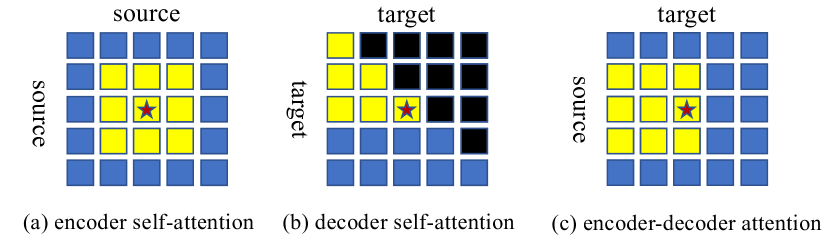
As illustrated by Figure 3(b), the decoder self-attention only takes upper-left pixels in the convolution. The upper-right pixels (black color) are permanently masked, while other pixels (blue color) are not calculated for the current token. This results in a convolution kernel with a receptive field of 6, which can be implemented as follows: (1) performing standard convolution with masks in the upper-right corner; (2) after convolution, shifting the entire attention matrix by 1 pixel to the bottom and 1 pixel to the right. As illustrated by Figure 3(c), the encoder-decoder attention only takes the left pixels in the convolution kernel to prevent information leakage. This can be implemented by a standard convolution with 1 pixel shifting to the right.
4 Experiments
4.1 Image Classification
| Model | #Params | #FLOPs | Top-1 | Top-5 |
|---|---|---|---|---|
| ResNet-34 | 21.8M | 7.4G | 73.79 | 91.43 |
| AA-ResNet-34 | 20.7M | 7.1G | 74.33 | 91.92 |
| EA-AA-ResNet-34 | 20.7M | 7.9G | 75.23 | 92.35 |
| ResNet-50 | 25.6M | 8.2G | 76.44 | 93.19 |
| AA-ResNet-50 | 25.8M | 8.3G | 77.70 | 93.80 |
| EA-AA-ResNet-50 | 25.8M | 8.7G | 78.22 | 94.21 |
| ResNet-101 | 44.5M | 15.6G | 77.87 | 93.89 |
| AA-ResNet-101 | 45.4M | 16.1G | 78.50 | 94.02 |
| EA-AA-ResNet-101 | 45.4M | 17.2G | 79.29 | 94.81 |
| ResNet-152 | 60.2M | 23.0G | 78.40 | 94.20 |
| AA-ResNet-152 | 61.6M | 23.8G | 79.10 | 94.60 |
| EA-AA-ResNet-152 | 61.6M | 25.7G | 79.63 | 94.85 |
AA-ResNet (Bello et al., 2019) demonstrated that traditional CNN models could benefit from attention mechanisms in computer vision. Here we take AA-ResNet as the backbone model for ImageNet classification. AA-ResNet concatenates the image representations computed by self-attentions and convolutional neural networks. Our EA-AA-ResNet architecture enhances the attention mechanism by bridging the attention maps from different layers and extracting generic attention patterns through convolutional modules.
Settings. We follow the experimental protocol of AA-ResNet which adds self-attention to standard ResNet architectures (He et al., 2016). We set and for EA-AA-ResNet-34, while a hyper-parameter analysis and the settings for other architectures can be found in the appendix. All models are trained by 1.28 million training images for 100 epochs on 8 TESLA V100 GPUs. Finally, we report the top-1 and top-5 accuracy on 50k validation images. Major hyper-parameters are as follows: optimizer is SGD with momentum 0.9, batch size is 32 per worker, weight decay is 1e-4. For the first 5 epochs, the learning rate is scaled linearly from 0 to 0.128, and then it is divided by 10 at epoch 30, 60, 80 and 90.
Results. As shown in Table 1, AA-ResNets consistently outperform corresponding ResNet baselines by a large margin. The proposed EA-AA-ResNets further boost the top-1 accuracy by 1.21%, 0.67%, 0.80% and 0.67% on top of AA-ResNet-34, -50, -101 and -152 respectively. These numbers are statistically significant under 95% confidence level. As demonstrated in Figure 1, the performance enhancement is consistent in different model capacities. Arguably, this is owing to better attention maps induced by the proposed evolving attention mechanism. We will show more evidences in the analysis section.
| Model | ImageNet Top-1 | Top-5 |
|---|---|---|
| AA-ResNet-34 | 74.33 | 91.92 |
| EA-AA-ResNet-34 | 75.23 | 92.35 |
| w/o Convolution | 74.34 | 91.98 |
| w/o Skip Connection | 74.29 | 91.85 |
| with Convolution | 74.99 | 92.20 |
| with Convolution | 75.12 | 92.55 |
Ablation Study. To understand the importance of each component, we conduct ablation experiments for the EA-AA-ResNet-34 architecture. In Table 2, w/o Convolution means removing the attention convolution module from EA-AA-ResNet (); w/o Skip Connection means removing skip connections between adjacent attention maps (); Besides, we also replace standard convolutions with or kernels. As indicated by the results, both convolutions and skip connections are crucial for the final performance. One can also notice a significant accuracy drop using convolutions (analogies to FFN), which indicates that a convolutional inductive bias is beneficial for capturing evolving attention patterns. Meanwhile, convolutions also work fairly well, but we prefer convolutions as they require fewer parameters.
4.2 Natural Language Understanding
| Model | #Params | #FLOPs | Avg | CoLA | SST-2 | MRPC | STS-B | QQP | MNLI-m/-mm | QNLI | RTE |
|---|---|---|---|---|---|---|---|---|---|---|---|
| BERT-Base | 109.5M | 6.3G | 80.9 | 51.7 | 93.5 | 87.2/82.1 | 86.7/85.4 | 91.1/89.0 | 84.3/83.7 | 90.4 | 67.2 |
| EA-BERT-Base | 110.4M | 6.8G | 83.3 | 60.0 | 93.8 | 89.1/84.2 | 89.6/89.5 | 91.6/88.4 | 85.2/85.5 | 92.1 | 69.0 |
| T5-Base | 220.2M | 9.1G | 83.4 | 53.1 | 92.2 | 92.0/88.7 | 89.1/88.9 | 88.2/91.2 | 84.7/85.0 | 91.7 | 76.9 |
| Synthesizer | 272.0M | 11.3G | 84.0 | 53.3 | 92.2 | 91.2/87.7 | 89.3/88.9 | 88.6/91.4 | 85.0/84.6 | 92.3 | 81.2 |
| EA-T5-Base | 221.2M | 9.9G | 84.5 | 53.7 | 93.1 | 92.3/89.0 | 89.6/89.1 | 88.8/91.9 | 85.1/85.0 | 92.3 | 81.5 |
| BERT-Large | 335.0M | 12.2G | 83.7 | 60.5 | 94.9 | 89.3/85.4 | 87.6/86.5 | 92.1/89.3 | 86.8/85.9 | 92.7 | 70.1 |
| RealFormer | 335.0M | 12.2G | 84.3 | 59.8 | 94.0 | 90.9/87.0 | 90.1/89.9 | 91.3/88.3 | 86.3/86.3 | 91.9 | 73.7 |
| EA-BERT-Large | 336.7M | 12.9G | 85.3 | 62.9 | 95.2 | 90.9/89.4 | 89.7/88.2 | 92.4/90.1 | 87.9/86.8 | 93.9 | 72.4 |
| RoBERTa-Large | 355.0M | 12.7G | 86.4 | 63.8 | 96.3 | 91.0/89.4 | 72.9/90.2 | 92.7/90.1 | 89.5/89.7 | 94.2 | 84.2 |
| EA-RoBERTa-Large | 356.7M | 13.3G | 87.2 | 65.8 | 96.4 | 91.8/90.8 | 73.8/90.3 | 93.3/90.2 | 90.5/89.8 | 95.2 | 85.0 |
Pre-trained language models like BERT become popular in recent years. These models are based on bi-directional transformer architectures and pre-trained by a large corpus. Our solution can be easily plugged into an existing checkpoint of vanilla BERT and achieve significant improvement through continuous training. To demonstrate this advantage, we choose GLUE benchmark (Wang et al., 2018) for an empirical study.
Settings. The encoder network of BERT consists of multiple transformer blocks. In EA-BERT, we replace each transformer block with EA-Transformer illustrated in Figure 2(b). We load the pre-trained checkpoints of BERT-Base, T5-Base, BERT-Large and RoBERTa-Large directly, and fine-tune them for each downstream task individually on the task-specific training data. The additional parameters introduced by EA-BERT are initialized randomly and trained jointly with other parameters during fine-tuning. We use the Adam optimizer (Kingma & Ba, 2014) with epsilon 1e-8. The dropout ratio is set as 0.1 empirically. Hyper-parameters are tuned in the following search space on the validation set: learning rate {1e-4, 1e-5, 2e-5}, batch size {8, 16}, training epochs {2, 3, 5}, {0.1, 0.2, 0.4} and {0.1, 0.2, 0.4}. The values of hyper-parameters chosen for each task will be reported in the appendix.
Results. The comparison between BERT-style models are shown in Table 3. The T5-Base and BERT-Large models are evaluated on the development set in order to be comparable with existing baselines. Other models are evaluated on the test set. EA-BERT generally performs better than vanilla BERT in different downstream tasks. Specifically, EA-BERT-Base, EA-T5-Base, EA-BERT-Large and EA-RoBERTa-Large achieve average scores of 83.3, 84.5, 85.0 and 87.2 on the GLUE benchmark, increasing 2.4, 1.1, 1.6 and 0.8 absolute points from the corresponding baselines respectively. The improvement can be achieved by loading an existing checkpoint and fine-tuning the extra parameters with limited training time, which is an appealing advantage in practice. In addition, it is worth mentioning that EA-BERT-Base boosts the score by 8.1 on CoLA dataset, indicating its superior generalization ability for small datasets. Moreover, the EA-based models demonstrate more benefits over two concurrent works, Realformer (He et al., 2020) and Synthesizer (Tay et al., 2020). Realformer utilizes residual connections over attention maps, but does not exploit convolution-based modules for evolving attention patterns. Synthesizer generates a separate attention map and mixes it with vanilla ones.
| Model | CoLA | SST-2 | MRPC | MNLI |
|---|---|---|---|---|
| BERT-Base | 51.7 | 93.5 | 87.2/82.1 | 84.3/83.7 |
| EA-BERT-Base | 60.0 | 93.8 | 89.1/84.2 | 85.2/85.5 |
| w/o Convolution | 52.1 | 93.6 | 87.6/82.8 | 84.5/84.0 |
| w/o Skip Connection | 52.9 | 93.5 | 87.4/82.4 | 84.3/83.8 |
| with Convolution | 57.5 | 93.6 | 88.4/83.4 | 84.7/84.8 |
| with Convolution | 59.2 | 93.6 | 89.0/83.9 | 85.2/85.4 |
Ablation Study We perform an ablation study for EA-BERT-Base on four text datasets with different data scales. According to the results in Table 4, the privilege of EA-BERT comes from both convolution-based pattern extraction and residual connections simultaneously. Removing the convolutional module or replacing it with kernel causes a significant performance drop. Skip connections are also advantageous, without which we only have small gains over the vanilla model. Similar to image classification, kernel also generates competitive results.
| Model | #Params | #FLOPs (En-De) | IWSLT’14 De-En | WMT’14 En-De | WMT’14 En-Fr |
|---|---|---|---|---|---|
| Transformer-Lite | 2.48M | 158.31M | 33.32 | 21.11 | 33.22 |
| EA-Transformer-Lite | 2.49M | 163.46M | 33.80 | 21.63 | 34.12 |
| Transformer-Base | 44.14M | 2.68G | 34.55 | 27.47 | 40.79 |
| EA-Transformer-Base | 44.15M | 2.70G | 35.30 | 27.56 | 41.54 |
| Model | De-En | En-De | En-Fr |
|---|---|---|---|
| Transformer-Lite | 33.21 | 21.11 | 33.22 |
| EA-Transformer-Lite | 33.80 | 21.63 | 34.12 |
| w/o Encoder Convolution | 32.84 | 21.07 | 33.51 |
| w/o Decoder Convolution | 33.56 | 21.45 | 33.72 |
| w/o Encoder-Decoder Convolution | 33.59 | 21.41 | 33.73 |
| w/o Skip Connection | 33.70 | 21.43 | 34.06 |
| with Convolution | 33.15 | 21.20 | 33.52 |
| with Convolution | 33.54 | 21.40 | 34.08 |
4.3 Machine Translation
Machine translation is a common benchmark for testing sequence to sequence architectures. In our experiments, we take three machine translation datasets: IWSLT’14 German-English (De-En), WMT’14 English to German (En-De) and WMT’14 English to French (En-Fr).
Settings. In an EA-Transformer, the convolution modules are applied to encoder self-attention, decoder self-attention and encoder-decoder attention separately. Skip connections are only used in the encoder network as we find they harm the performance of a decoder. We set for EA-Transformer-Lite and for EA-Transformer-Base. We adopt Adam optimizer with , and an inverse square root learning rate scheduling with linear warm-up. Warm-up step is set to be 4000 and label smoothing is 0.1. For each task, we tune the learning rate from {1e-4, 5e-4, 1e-3} and dropout ratio from {0.1, 0.2, 0.3}, which will be reported in the appendix.
Results. We compare Transformer and EA-Transformer with different model capacities. Transformer-Lite (Wu et al., 2020) is a light architecture where all dimensions are set as 160 to replace a bottleneck structure. Transformer-Base follows the configuration in Vaswani et al. (2017), which has six layers for the encoder and 6 layers for the decoder network. It has 8 heads, 512 dimension for normal layers and 2048 dimension for the first FFN layer, forming a bottleneck structure. As illustratged in Table 5, EA-based models achieve consistent improvement for multiple datasets and network architectures while requiring only a few extra parameters and computations.
Ablation Study. The ablation results of EA-Transformer-Lite are listed in Table 6. First, we remove the convolutional modules for encoder, decoder, and encoder-decoder attentions respectively. As a result, the convolutional module is extremely important for the encoder network. It also has positive effects on decoder self-attention and encoder-decoder attentions. Consistent with previous conclusions, replacing convolutions with kernels leads to a huge decay in BLUE score. Therefore, the locality inductive bias is indefensible for a transformer model to evolve for better attention structures.
5 Analysis


5.1 Quality of Attention Maps
| Models | 16th Layer | 17th Layer | 18th Layer |
|---|---|---|---|
| AA-ResNet-34 | 24.50 | 31.18 | 17.55 |
| EA-AA-ResNet-34 | 31.02 | 31.71 | 31.93 |
To examine the quality of image attention maps, we select the middle attention layers (16th, 17th and 18th) in the 34-layers network for analysis. We take the attention maps centered on the middle pixel, the shape of which is , where is the image length (after pooling) and is the number of heads. We take these attention maps as direct inputs to another CNN model for classification. If the key structures are better captured in the attention maps, we should get higher accuracy scores for this task. As shown in Table 7, AA-ResNet-34 does not generate precise attention maps for the 16th and 18th layers, as the classification accuracy is relatively low. Instead, EA-AA-ResNet-34 induces good attention maps for all three layers, indicating the superiority of evolving attention.
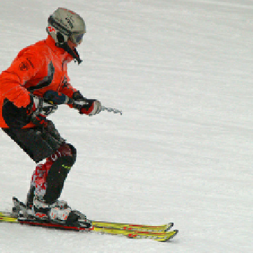
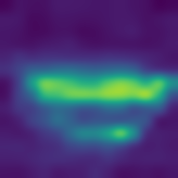
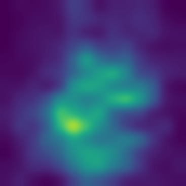
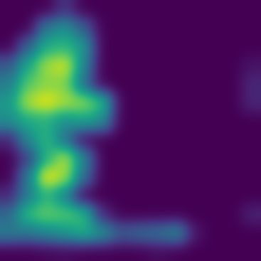
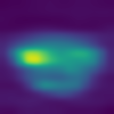
Figure 4 shows three exemplar cases for ImageNet classification, where the attention maps from representative heads of the 16th, 17th and 18th layers are visualized. These layers are at the middle of the network, which correspond to an appropriate abstraction level for visualization. Notably, AA-ResNet prefers to extract broad and vague attention patterns. In contrast, EA-AA-ResNet generates much sharper attention maps, and there exists a clear evolutionary trend in three consecutive layers. For the skier case, the attention map has successfully captured the main object in the 16th layer. Then, the outline becomes much clearer at the 17th layer with the assistance of evolving attention. Finally, the 18th layer is further improved as it identifies a complete skateboard. Other cases demonstrate a similar phenomenon.
| Dataset | Model | Perf. | AUPRC | Comp. | Suff. |
|---|---|---|---|---|---|
| Movie Reviews | BERT | 0.970 | 0.280 | 0.187 | 0.093 |
| EA-BERT | 0.975 | 0.313 | 0.194 | 0.089 | |
| FEVER | BERT | 0.870 | 0.291 | 0.212 | 0.014 |
| EA-BERT | 0.886 | 0.307 | 0.236 | 0.014 | |
| MultiRC | BERT | 0.655 | 0.208 | 0.213 | -0.079 |
| EA-BERT | 0.674 | 0.221 | 0.241 | -0.089 | |
| CoS-E | BERT | 0.487 | 0.544 | 0.223 | 0.143 |
| EA-BERT | 0.491 | 0.552 | 0.231 | 0.140 | |
| e-SNLI | BERT | 0.960 | 0.399 | 0.177 | 0.396 |
| EA-BERT | 0.969 | 0.534 | 0.445 | 0.368 |
5.2 Interpretability
A good model should generate not only correct predictions, but also give faithful reasons to explain the decisions. The ERASER benchmark (DeYoung et al., 2020) is proposed to evaluate the faithfulness of rationales for text representation models. Following the original setting, we adopt BERT+LSTM and EA-BERT+LSTM as the text representation models respectively, and utilize a state-of-the-art method, LIME (Ribeiro et al., 2016) to generate rationales for each model. The experimental results are listed in Table 8. It should be noted that higher comprehensiveness scores and lower sufficiency scores are desired. According to the results, the rationales given by evolving attention-based models are more accurate than those generated by vanilla ones. Thus, the evolving attention mechanism not only boosts the performances of text understanding models, but also improves their interpretability through inducing better attention maps.
5.3 Learning Curve Comparison
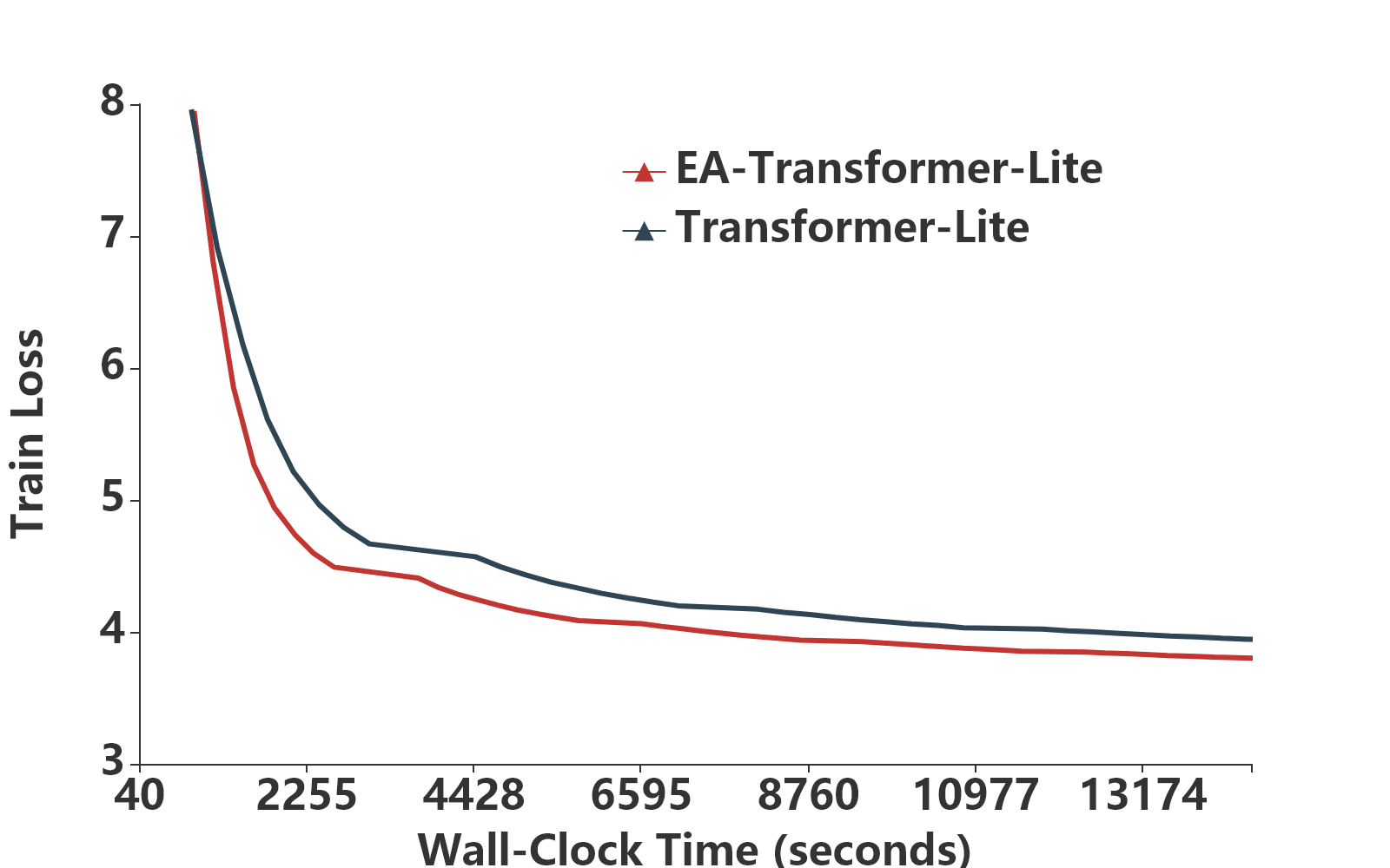
To demonstrate the efficiency of EA-Transformer, we further compare the learning curves of Transformer-Lite and EA-Transformer-Lite on IWSLT’14 De-En dataset. As shown in Figure 5, EA-Transformer-Lite always achieves lower training loss at the same wall-clock time, although it contains relatively 3% more FLOPs in each iteration. Finally, EA-Transformer-Lite achieves better training loss and BLUE score at convergence.
6 Conclusion
In this paper, we propose a novel mechanism, Evolving Attention for Transformers, which facilitates the learning of attention maps via a chain of residual convolutional neural networks. It obtains superior performance in various tasks in both CV and NLP domains. Future works are considered in three aspects. First, we will apply evolving attention to more tasks and domains, such as object detection, question answering and time-series forecasting. Second, we aim to investigate other modules instead of convolutions to capture generic patterns in attention maps. Last but not least, we would like to explore bi-directional decoders that benefit more from convolutions.
References
- Bello et al. (2019) Bello, I., Zoph, B., Vaswani, A., Shlens, J., and Le, Q. V. Attention augmented convolutional networks. In Proceedings of the IEEE International Conference on Computer Vision (ICCV), pp. 3286–3295, 2019.
- Devlin et al. (2019) Devlin, J., Chang, M.-W., Lee, K., and Toutanova, K. Bert: Pre-training of deep bidirectional transformers for language understanding. In North American Chapter of the Association for Computational Linguistics: Human Language Technologies (NAACL-HLT), 2019.
- DeYoung et al. (2020) DeYoung, J., Jain, S., Rajani, N. F., Lehman, E., Xiong, C., Socher, R., and Wallace, B. C. ERASER: A benchmark to evaluate rationalized NLP models. In Proceedings of the 58th Annual Meeting of the Association for Computational Linguistics (ACL), pp. 4443–4458, 2020.
- Dosovitskiy et al. (2020) Dosovitskiy, A., Beyer, L., Kolesnikov, A., Weissenborn, D., Zhai, X., Unterthiner, T., Dehghani, M., Minderer, M., Heigold, G., Gelly, S., et al. An image is worth 16x16 words: Transformers for image recognition at scale. arXiv preprint arXiv:2010.11929, 2020.
- Gehring et al. (2017) Gehring, J., Auli, M., Grangier, D., Yarats, D., and Dauphin, Y. N. Convolutional sequence to sequence learning. In International Conference on Machine Learning (ICML), pp. 1243–1252, 2017.
- He et al. (2016) He, K., Zhang, X., Ren, S., and Sun, J. Deep residual learning for image recognition. In Proceedings of the IEEE Conference on Computer Vision and Pattern Recognition (CVPR), pp. 770–778, 2016.
- He et al. (2020) He, R., Ravula, A., Kanagal, B., and Ainslie, J. Realformer: Transformer likes residual attention, 2020.
- Huang et al. (2017) Huang, G., Liu, Z., Van Der Maaten, L., and Weinberger, K. Q. Densely connected convolutional networks. In Proceedings of the IEEE Conference on Computer Vision and Pattern Recognition (CVPR), pp. 4700–4708, 2017.
- Jain & Wallace (2019) Jain, S. and Wallace, B. C. Attention is not explanation. In North American Chapter of the Association for Computational Linguistics: Human Language Technologies (NAACL-HLT), pp. 3543–3556, 2019.
- Kingma & Ba (2014) Kingma, D. P. and Ba, J. Adam: A method for stochastic optimization. arXiv preprint arXiv:1412.6980, 2014.
- Kitaev et al. (2020) Kitaev, N., Kaiser, L., and Levskaya, A. Reformer: The efficient transformer. In International Conference on Learning Representations (ICLR), 2020.
- Li et al. (2019) Li, S., Jin, X., Xuan, Y., Zhou, X., Chen, W., Wang, Y.-X., and Yan, X. Enhancing the locality and breaking the memory bottleneck of transformer on time series forecasting. In Advances in Neural Information Processing Systems (NeurIPS), pp. 5243–5253, 2019.
- Liu et al. (2019) Liu, Y., Ott, M., Goyal, N., Du, J., Joshi, M., Chen, D., Levy, O., Lewis, M., Zettlemoyer, L., and Stoyanov, V. Roberta: A robustly optimized BERT pretraining approach. CoRR, abs/1907.11692, 2019. URL http://arxiv.org/abs/1907.11692.
- Parmar et al. (2018) Parmar, N., Vaswani, A., Uszkoreit, J., Kaiser, L., Shazeer, N., Ku, A., and Tran, D. Image transformer. In International Conference on Machine Learning (ICML), 2018.
- Parmar et al. (2019) Parmar, N., Ramachandran, P., Vaswani, A., Bello, I., Levskaya, A., and Shlens, J. Stand-alone self-attention in vision models. In Advances in Neural Information Processing Systems (NeurIPS), pp. 68–80, 2019.
- Raffel et al. (2019) Raffel, C., Shazeer, N., Roberts, A., Lee, K., Narang, S., Matena, M., Zhou, Y., Li, W., and Liu, P. J. Exploring the limits of transfer learning with a unified text-to-text transformer. arXiv preprint arXiv:1910.10683, 2019.
- Raganato et al. (2018) Raganato, A., Tiedemann, J., et al. An analysis of encoder representations in transformer-based machine translation. In EMNLP Workshop BlackboxNLP: Analyzing and Interpreting Neural Networks for NLP, 2018.
- Ribeiro et al. (2016) Ribeiro, M. T., Singh, S., and Guestrin, C. “why should i trust you?”: Explaining the predictions of any classifier. In Proceedings of the 2016 Conference of the North American Chapter of the Association for Computational Linguistics: Demonstrations, pp. 97–101, 2016.
- Shaw et al. (2018) Shaw, P., Uszkoreit, J., and Vaswani, A. Self-attention with relative position representations. In North American Chapter of the Association for Computational Linguistics: Human Language Technologies (NAACL-HLT), pp. 464–468, 2018.
- Shiv & Quirk (2019) Shiv, V. and Quirk, C. Novel positional encodings to enable tree-based transformers. In Advances in Neural Information Processing Systems (NeurIPS), pp. 12081–12091, 2019.
- So et al. (2019) So, D., Le, Q., and Liang, C. The evolved transformer. In International Conference on Machine Learning (ICML), pp. 5877–5886, 2019.
- Sukhbaatar et al. (2019) Sukhbaatar, S., Grave, É., Bojanowski, P., and Joulin, A. Adaptive attention span in transformers. In Proceedings of the 57th Annual Meeting of the Association for Computational Linguistics (ACL), pp. 331–335, 2019.
- Szegedy et al. (2016) Szegedy, C., Vanhoucke, V., Ioffe, S., Shlens, J., and Wojna, Z. Rethinking the inception architecture for computer vision. In Proceedings of the IEEE conference on computer vision and pattern recognition (CVPR), pp. 2818–2826, 2016.
- Tang et al. (2018) Tang, G., Müller, M., Gonzales, A. R., and Sennrich, R. Why self-attention? a targeted evaluation of neural machine translation architectures. In Empirical Methods in Natural Language Processing (EMNLP), 2018.
- Tay et al. (2020) Tay, Y., Bahri, D., Metzler, D., Juan, D.-C., Zhao, Z., and Zheng, C. Synthesizer: Rethinking self-attention in transformer models. arXiv preprint arXiv:2005.00743, 2020.
- Vaswani et al. (2017) Vaswani, A., Shazeer, N., Parmar, N., Uszkoreit, J., Jones, L., Gomez, A. N., Kaiser, Ł., and Polosukhin, I. Attention is all you need. In Advances in Neural Information Processing Systems (NeurIPS), pp. 5998–6008, 2017.
- Wang et al. (2018) Wang, A., Singh, A., Michael, J., Hill, F., Levy, O., and Bowman, S. R. Glue: A multi-task benchmark and analysis platform for natural language understanding. In International Conference on Learning Representations (ICLR), 2018.
- Wiegreffe & Pinter (2019) Wiegreffe, S. and Pinter, Y. Attention is not not explanation. In Empirical Methods in Natural Language Processing (EMNLP), pp. 11–20, 2019.
- Wolf et al. (2019) Wolf, T., Debut, L., Sanh, V., Chaumond, J., Delangue, C., Moi, A., Cistac, P., Rault, T., Louf, R., Funtowicz, M., Davison, J., Shleifer, S., von Platen, P., Ma, C., Jernite, Y., Plu, J., Xu, C., Scao, T. L., Gugger, S., Drame, M., Lhoest, Q., and Rush, A. M. Huggingface’s transformers: State-of-the-art natural language processing. ArXiv, abs/1910.03771, 2019.
- Wu et al. (2020) Wu, Z., Liu, Z., Lin, J., Lin, Y., and Han, S. Lite transformer with long-short range attention. In International Conference on Learning Representations (ICLR), 2020.
Appendix A Settings for reproduction
A.1 Image classification
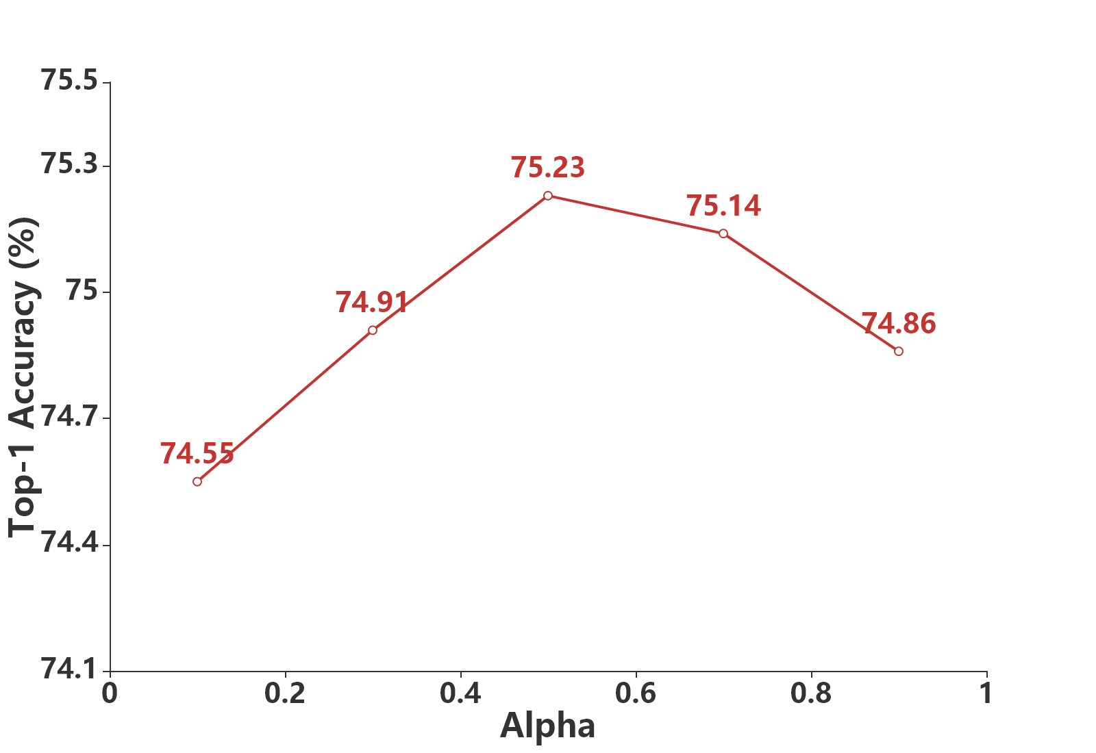
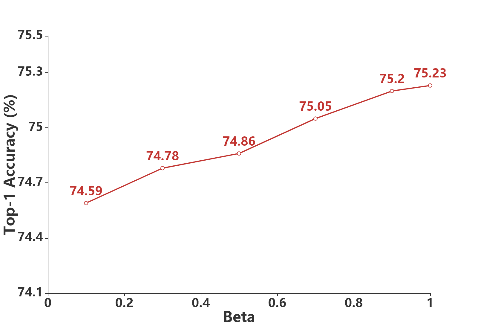
We follow a common strategy described in Szegedy et al. (2016) for data augmentation. For ResNet (He et al., 2016), we adopt the implementation in tensorflow 111https://github.com/tensorflow/models/tree/v1.13.0. For AA-ResNet, we modify the ResNet by augmenting 3x3 convolution with self-attention. The implementation is from the official repository of AA-ResNet222https://github.com/leaderj1001/Attention-Augmented-Conv2d, while we simply add the residual convolution module for EA-AA-ResNet. Concretely, we apply attention augmentation to each residual block in the last three stages – when the shapes of activation maps become 28x28, 14x14 and 7x7. We adopt the same setting as AA-ResNet, e.g. and . We refer to (Bello et al., 2019) for more details. We set and by default, except for EA-AA-ResNet-152 and EA-AA-ResNet-101 where we set . A hyper-parameter analysis for and in EA-AA-ResNet-34 is shown in Figure 6. We can see that the best result is achieved at and , which significantly outperforms the vanilla transformer (equivalent to and ).
| Model | Task | Training Epochs | Batch Size | Learning Rate | Adam Epsilon | Dropout Rate | ||
|---|---|---|---|---|---|---|---|---|
| BERT-Base | CoLA | 3 | 8 | 2e-5 | 1e-8 | 0.1 | 0.2 | 0.1 |
| SST-2 | 5 | 8 | 1e-5 | 1e-8 | 0.1 | 0.1 | 0.1 | |
| MRPC | 2 | 8 | 2e-5 | 1e-8 | 0.1 | 0.1 | 0.2 | |
| STS-B | 3 | 8 | 2e-5 | 1e-8 | 0.1 | 0.2 | 0.2 | |
| QQP | 3 | 16 | 2e-5 | 1e-8 | 0.1 | 0.1 | 0.2 | |
| MNLI | 3 | 16 | 2e-5 | 1e-8 | 0.1 | 0.1 | 0.2 | |
| QNLI | 3 | 16 | 2e-5 | 1e-8 | 0.1 | 0.1 | 0.1 | |
| RTE | 2 | 8 | 2e-5 | 1e-8 | 0.1 | 0.2 | 0.1 | |
| WNLI | 2 | 8 | 2e-5 | 1e-8 | 0.1 | 0.2 | 0.2 | |
| BERT-Large | CoLA | 3 | 8 | 2e-5 | 1e-8 | 0.1 | 0.1 | 0.2 |
| SST-2 | 5 | 8 | 1e-5 | 1e-8 | 0.1 | 0.1 | 0.2 | |
| MRPC | 2 | 8 | 1e-5 | 1e-8 | 0.1 | 0.1 | 0.1 | |
| STS-B | 3 | 8 | 2e-5 | 1e-8 | 0.1 | 0.1 | 0.2 | |
| QQP | 3 | 16 | 1e-5 | 1e-8 | 0.1 | 0.1 | 0.1 | |
| MNLI | 3 | 16 | 2e-5 | 1e-8 | 0.1 | 0.2 | 0.2 | |
| QNLI | 3 | 16 | 2e-5 | 1e-8 | 0.1 | 0.2 | 0.2 | |
| RTE | 3 | 16 | 1e-4 | 1e-8 | 0.1 | 0.1 | 0.2 | |
| WNLI | 2 | 8 | 2e-5 | 1e-8 | 0.1 | 0.2 | 0.2 | |
| RoBERTa-Large | CoLA | 3 | 8 | 2e-5 | 1e-8 | 0.1 | 0.2 | 0.1 |
| SST-2 | 5 | 8 | 1e-5 | 1e-8 | 0.1 | 0.1 | 0.2 | |
| MRPC | 3 | 16 | 1e-5 | 1e-8 | 0.1 | 0.1 | 0.2 | |
| STS-B | 3 | 16 | 2e-5 | 1e-8 | 0.1 | 0.4 | 0.2 | |
| QQP | 3 | 16 | 2e-5 | 1e-8 | 0.1 | 0.1 | 0.1 | |
| MNLI | 5 | 16 | 1e-5 | 1e-8 | 0.1 | 0.4 | 0.1 | |
| QNLI | 5 | 16 | 1e-5 | 1e-8 | 0.1 | 0.4 | 0.2 | |
| RTE | 2 | 8 | 1e-4 | 1e-8 | 0.1 | 0.2 | 0.4 | |
| WNLI | 2 | 8 | 2e-5 | 1e-8 | 0.1 | 0.2 | 0.1 | |
| T5-Base | CoLA | 3 | 8 | 2e-5 | 1e-8 | 0.1 | 0.2 | 0.2 |
| SST-2 | 3 | 8 | 2e-5 | 1e-8 | 0.1 | 0.1 | 0.2 | |
| MRPC | 3 | 8 | 1e-4 | 1e-8 | 0.1 | 0.1 | 0.1 | |
| STS-B | 3 | 16 | 2e-5 | 1e-8 | 0.1 | 0.1 | 0.1 | |
| QQP | 3 | 16 | 2e-5 | 1e-8 | 0.1 | 0.1 | 0.2 | |
| MNLI | 5 | 16 | 1e-5 | 1e-8 | 0.1 | 0.1 | 0.1 | |
| QNLI | 5 | 16 | 1e-5 | 1e-8 | 0.1 | 0.2 | 0.1 | |
| RTE | 3 | 16 | 1e-5 | 1e-8 | 0.1 | 0.4 | 0.2 | |
| WNLI | 2 | 8 | 2e-5 | 1e-8 | 0.1 | 0.2 | 0.2 |
A.2 Natural language understanding
As introduced in (Devlin et al., 2019), BERT-Base and EA-BERT-Base have 12 layers and 12 attention heads with hidden dimension 768. BERT-large and EA-BERT-large have 24 layers and 16 heads, while hidden dimension for each intermediate layer is set as 1024. The hidden dimension of the final fully-connected layer before softmax is set to be 2000. We download the official checkpoints of BERT-Base333https://storage.googleapis.com/bert_models/2018_10_18/uncased_L-12_H-768_A-12.zip and BERT-Large444https://storage.googleapis.com/bert_models/2018_10_18/uncased_L-24_H-1024_A-16.zip, and initialize the additional parameters for EA-BERT-Base and EA-BERT-Large randomly.
We also conduct a set of experiments with RoBERTa-Large (Liu et al., 2019) and T5-Base (Raffel et al., 2019). We apply the idea of evolving attention to the network of these models. RoBERTa-Large has 24 layers with 16 attention heads. The total hidden size of all heads is 1024, and the hidden dimension of the final fully-connected layer is 4096. We use NLP library implemented by the huggingface team (Wolf et al., 2019) to implement the base version of T5, which has 220 million parameter. We download the official pre-trained checkpoints for RoBERTa-Large555https://dl.fbaipublicfiles.com/fairseq/models/roberta.large.tar.gz and T5-Base666https://console.cloud.google.com/storage/browser/t5-data/pretrained_models/base/ for fine-tuning.
We adopt the Adam optimizer (Kingma & Ba, 2014) with epsilon 1e-8. The dropout rate is set as 0.1 empirically. We use grid search to optimize the values of hyper-parameters on the validation set. We search the learning rate in {1e-4, 1e-5, 2e-5}, batch size in {8, 16}, training epochs in {2, 3, 5}, in {0.1, 0.2, 0.4} and in {0.1, 0.2, 0.4}. The specific hyper-parameters for each task are listed in Table 9.
| Model | Task | Number of GPU | Accumulative Steps | Learning Rate | Dropout Rate | ||
|---|---|---|---|---|---|---|---|
| EA-Transformer-Lite | De-En | 1 | 1 | 1e-3 | 0.2 | 0.1 | 0.1 |
| En-De | 8 | 16 | 1e-3 | 0.3 | 0.1 | 0.1 | |
| En-Fr | 8 | 16 | 1e-3 | 0.1 | 0.1 | 0.1 | |
| EA-Transformer-Base | De-En | 1 | 1 | 1e-3 | 0.2 | 0.5 | 0.1 |
| En-De | 8 | 16 | 1e-3 | 0.3 | 0.5 | 0.1 | |
| En-Fr | 8 | 16 | 1e-3 | 0.1 | 0.5 | 0.1 |
A.3 Machine Translation
We train the machine translation tasks using Adam optimizer (Kingma & Ba, 2014) with , and an inverse square root learning rate scheduling with linear warmup. The learning rate is 1e-3 and the warmup step is set to be 4000. Also, we use label smoothing . we apply early stopping to the training procedure with a patience of 5 epochs. In the evaluation phase, we average the final 10 checkpoints and conduct beam search with size 5. We adopt absolute positional encoding according to the original implementation (Vaswani et al., 2017). Other hyper-parameters are optimized by grid search on the validation set and reported in Table 10.
| Perf. | AUPRC | Comp. | Suff. | |
|---|---|---|---|---|
| Movie Reviews | ||||
| BERT+LSTM - Attention | 0.970 | 0.417 | 0.129 | 0.097 |
| BERT+LSTM - EA-Attention | 0.970 | 0.435 | 0.142 | 0.084 |
| BERT+LSTM - Lime | 0.970 | 0.280 | 0.187 | 0.093 |
| EA-BERT+LSTM -Lime | 0.975 | 0.313 | 0.194 | 0.089 |
| FEVER | ||||
| BERT+LSTM - Attention | 0.870 | 0.235 | 0.037 | 0.122 |
| BERT+LSTM - EA-attention | 0.870 | 0.238 | 0.078 | 0.097 |
| BERT+LSTM - Lime | 0.870 | 0.291 | 0.212 | 0.014 |
| EA-BERT+LSTM -Lime | 0.886 | 0.307 | 0.236 | 0.014 |
| MultiRC | ||||
| BERT+LSTM - Attention | 0.655 | 0.244 | 0.036 | 0.052 |
| BERT+LSTM - EA-Attention | 0.655 | 0.251 | 0.054 | 0.041 |
| BERT+LSTM - Lime | 0.655 | 0.208 | 0.213 | -0.079 |
| EA-BERT+LSTM -Lime | 0.674 | 0.221 | 0.241 | -0.089 |
| CoS-E | ||||
| BERT+LSTM - Attention | 0.487 | 0.606 | 0.080 | 0.217 |
| BERT+LSTM - EA-Attention | 0.487 | 0.610 | 0.113 | 0.189 |
| BERT+LSTM - Lime | 0.487 | 0.544 | 0.223 | 0.143 |
| EA-BERT+LSTM -Lime | 0.491 | 0.552 | 0.231 | 0.140 |
| e-SNLI | ||||
| BERT+LSTM - Attention | 0.960 | 0.395 | 0.105 | 0.583 |
| BERT+LSTM - EA-Attention | 0.960 | 0.399 | 0.177 | 0.396 |
| BERT+LSTM - Lime | 0.960 | 0.513 | 0.437 | 0.389 |
| EA-BERT+LSTM -Lime | 0.969 | 0.534 | 0.445 | 0.368 |
Appendix B Analysis
B.1 Quality of Image Attention
We select the 16th, 17th and 18th attention layers in the AA-ResNet-34 and EA-AA-ResNet34 networks for analysis. The attention maps from these layers have a shape of , where 14 is the image length after pooling and 8 is the number of heads. Then, we send the attention maps directly as inputs to another CNN model for classification, and the original labels are used for training and evaluation. The goal is to quantify the effectiveness of attention maps learned by different models. If an attention map retains major structures of the original object, the classification accuracy should be higher. We adopt a 12-layer DenseNet (Huang et al., 2017) for attention map classification, while the shape is pooled to and after the 4th and 7th layers respectively. The hidden dimension is set as 256 initially and doubled after each pooling operation. The models are trained by 30 epochs with cosine learning rate decay started by 0.05 and ended by 0.0001.
B.2 Interpretability
In the context of modern neural models, attention mechanisms learn to assign soft weights to token representations, thus one can extract highly weighted tokens as rationales. In other words, if the self-attention mechanism generates better attention scores, it will achieve better performance on ERASER, a benchmark designed to evaluate the interpretability of natural language understanding models. We list the experimental results on the ERASER benchmark in Table 11. It should be noted that higher comprehensiveness scores and lower sufficiency scores are desired. First, we consider a text representation model that passes tokens through BERT and a bidirectional LSTM. Based on the same text representation, we use different methods for rationale generation. Here, the models are the same, so the downstream performance is equivalent. According to the experimental results, the rationales generated using evolving attention are more accurate than the ones generated by vanilla attention. Next, we replace vanilla BERT with EA-BERT as the text representation model and utilize a state-of-the-art rationale generation method, Lime (Ribeiro et al., 2016). Experimental results show that EA-BERT improves the performances of downstream tasks and generates better rationales simultaneously.
Appendix C Case Study
In order to get insight into the evolving attention mechanism, we visualize exemplar attention maps for both text and image inputs and find some interesting evidences.
C.1 Image attention
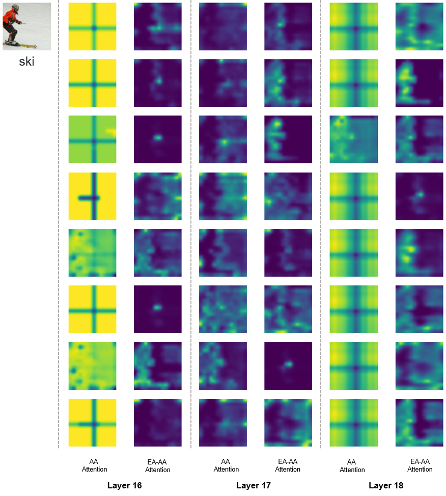
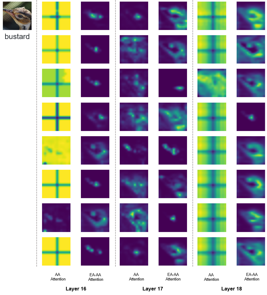
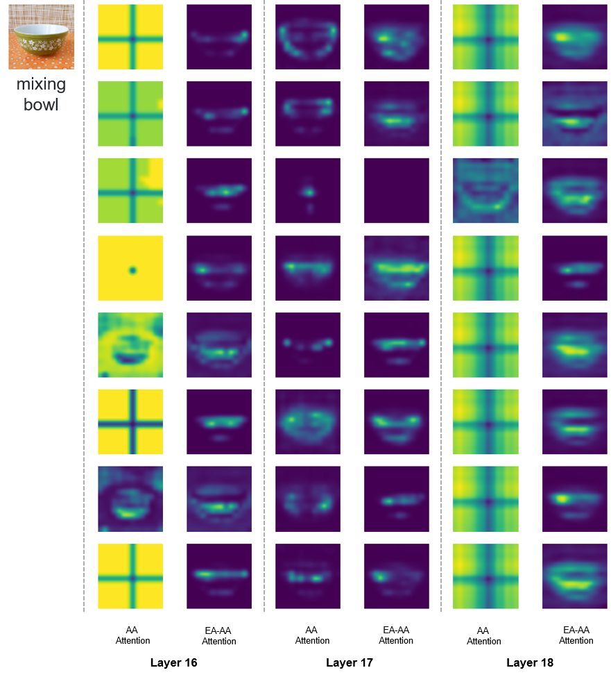
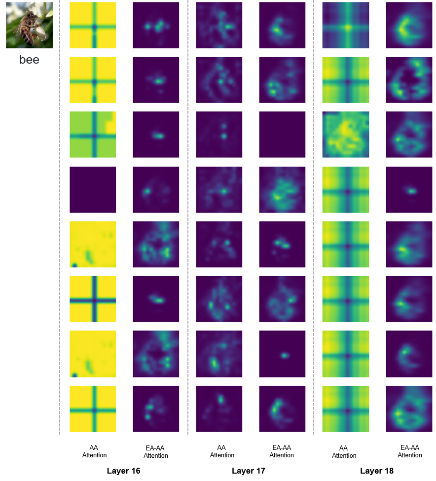
In Figure 7-10, we compare the attention maps of AA-ResNet-34 and EA-AA-ResNet-34 for ImageNet classification. Compared to AA-ResNet, our proposed convolution-based evolving attention mechanism captures better global information and at the same time emphasizes on the important local information. Specifically, the residual connections and convolutional inductive bias assist the self-attention mechanism to depict a more clear outline. As shown by the visualized examples, AA-ResNet fails to compute a explainable attention map for some layers. In contrast, with the help of residual convolutions, EA-AA-ResNet successfully identifies the objects in images in an evolving process.
C.2 Text Attention
We choose BERT-Base and EA-BERT-Base models for comparison on the CoLA dataset, a task of judging the grammatical correctness of a sentence. We select the sentence “Mary tried John to go abroad.” for a case study. Obviously, this sentence is grammatically wrong, and a model should capture the error part “tried John to” in order to give the correct answer.
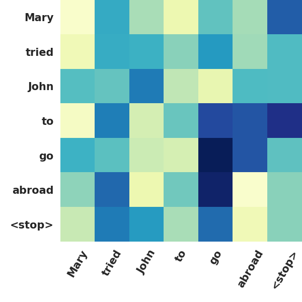
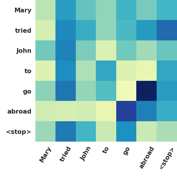
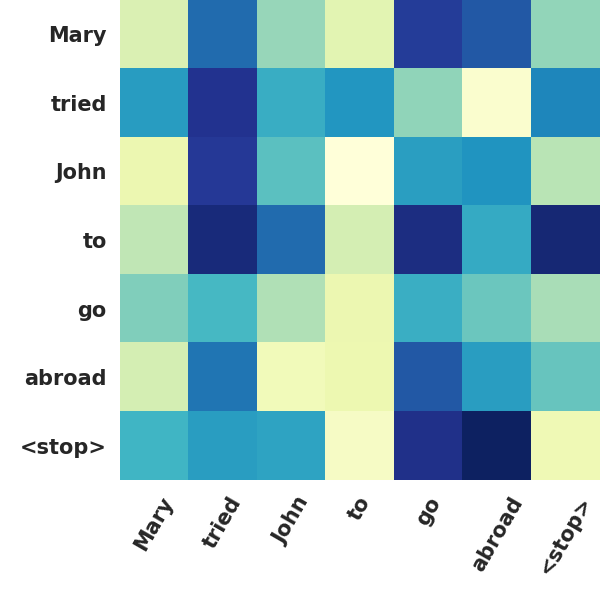
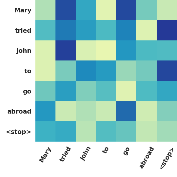

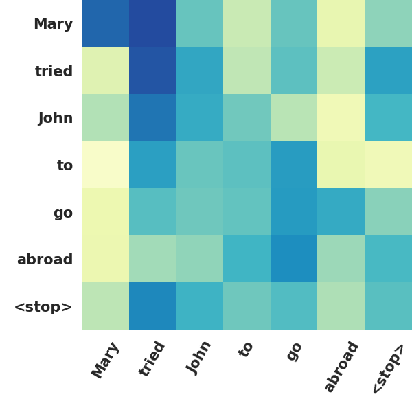
In Figure 11, we visualize related attention maps for three layers (#2, #11 and #12) in BERT-Base and EA-BERT-Base models. The second layer is the first layer that utilizes residual attention, and #11 and #12 are the last two layers. For each layer, we first show the attention maps from vanilla BERT and EA-BERT in the first and second columns respectively, then the convolution-based attention and self-attention maps are visualized in the third and fourth column. It should be noted that the second column is the linear fusion result of the third column and the fourth column.
Consider layer #2, both BERT (Figure 11(a)) and EA-BERT (Figure 11(b)) pay major attentions on the verb phrase “go abroad”. As shown in Figure 11(b), EA-BERT puts additional stress on the relation between word “tried” and the stop sign. This is reasonable because the stop sign is responsible of capturing sentence-level semantics and “tried” is a key word leading to the grammatical error. As shown in Figure 11(c), the attention on this part actually comes from the convolution-based module, which is sometimes complementary to the self-attention map.
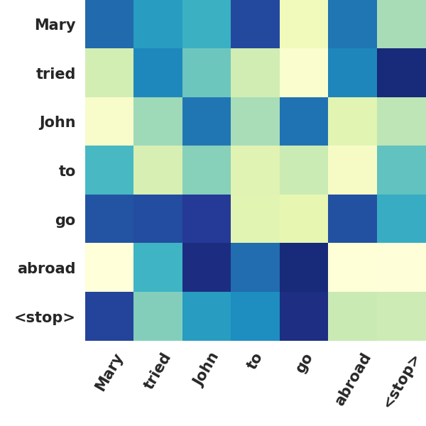
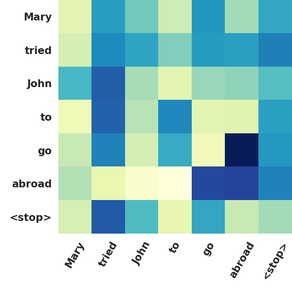
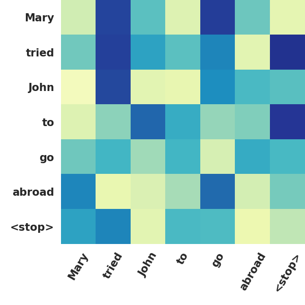
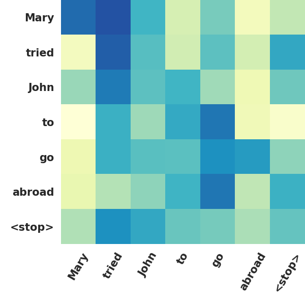
In order to ensure that the information obtained by the convolution is beneficial, we visualize the last attention layer (#12) which is the closest to the output (see Figure 11(i-l)). In Figure 11(i), we can observe that BERT-Base still focuses on verbs and stop signs in the very last layer of transformer. The attention to the wrong phrase “tried John” is still relatively weak, leading to a mis-classification result. In contrast, the attention scores between “tried” and “John” become obvious in EA-BERT (Figure 11(j)), largely owning to the convolutional attention map illustrated in Figure 11(k).
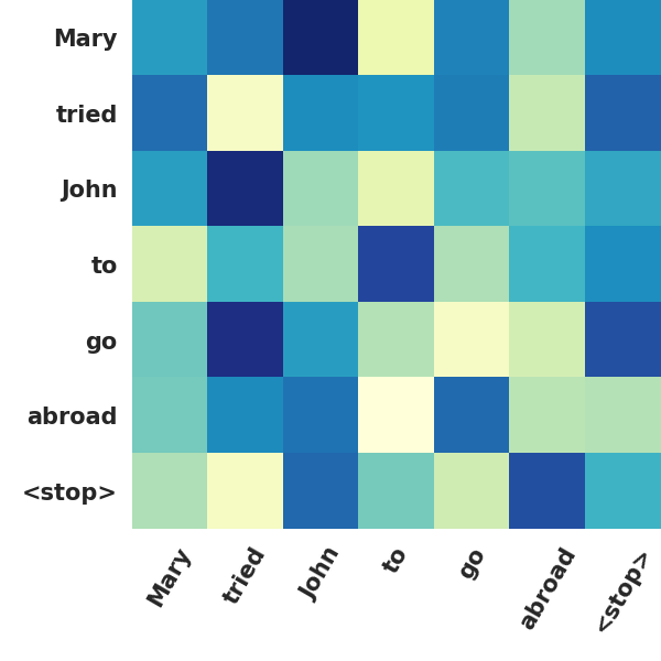
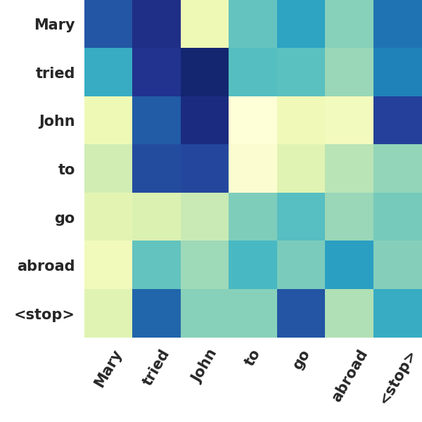
We also visualize the attention maps of the #11 layer, which serves as input to the #12 layer. To analysis the evolution of attention maps, we compare the differences between Figure 11(f) and Figure 11(k), as the latter is the evolved attention map taking the former as input. We find that the convolutional module helps to reason about the important word relations based on the previous attention maps. Specifically, it weakens the attention scores of the correct parts and raises higher scores for the wrong parts. As illustrated in Figure 11(k), the attention scores are significant in the upper left corner of the matrix where the error occurs. In this way, the error is fully captured in the final representation layer, helping EA-BERT to generate a correct answer.