FASA: Feature Augmentation and Sampling Adaptation
for Long-Tailed Instance Segmentation

Abstract

Recent methods for long-tailed instance segmentation still struggle on rare object classes with few training data. We propose a simple yet effective method, Feature Augmentation and Sampling Adaptation (FASA), that addresses the data scarcity issue by augmenting the feature space especially for rare classes. Both the Feature Augmentation (FA) and feature sampling components are adaptive to the actual training status — FA is informed by the feature mean and variance of observed real samples from past iterations, and we sample the generated virtual features in a loss-adapted manner to avoid over-fitting. FASA does not require any elaborate loss design, and removes the need for inter-class transfer learning that often involves large cost and manually-defined head/tail class groups. We show FASA is a fast, generic method that can be easily plugged into standard or long-tailed segmentation frameworks, with consistent performance gains and little added cost. FASA is also applicable to other tasks like long-tailed classification with state-of-the-art performance.

1 Introduction

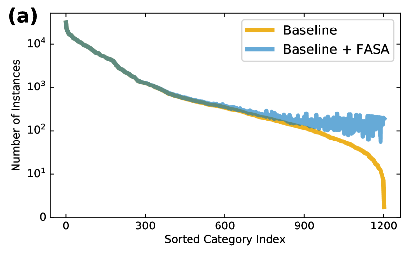
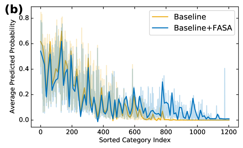
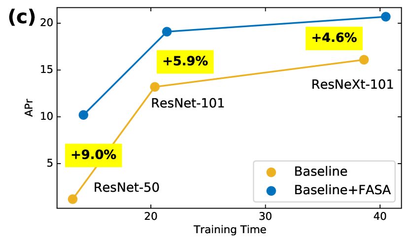
Figure 1: Class imbalance and the comparison of Mask R-CNN [16] baseline with and without FASA on LVIS v1.0 dataset. (a) By adaptive feature augmentation and sampling, our method FASA largely alleviates the imbalance issue, especially for rare classes. (b) Compare the prediction results of FASA vs Mask R-CNN baseline regarding average category probability scores. The baseline model predicts near-zero scores for rare classes. While with FASA, rare-class scores are significantly boosted which merits final performance. (c) FASA brings consistent improvements over different backbone models in mask AP${}_{\textrm{r}}$ defined on rare classes. Such gains come at a very low cost (training time only increases by $\sim 3\%$ on average).

A growing number of methods are proposed to learn from long-tailed data in vision tasks like face recognition [19], image classification [31] and instance segmentation [15]. We focus on the problem of long-tailed instance segmentation, which is particularly challenging due to the class imbalance issue. State-of-the-art methods [2, 5, 16, 27] often fail to handle this issue and witness a large performance drop on rare object classes. Fig. 1 exemplifies the struggle of the competitive Mask R-CNN [16] baseline on highly imbalanced LVIS v1.0 dataset [15]. We can see that there are about 300 rare classes in the tail that have no more than $10^{2}$ positive object instances. Such scarce training data result in poor performance for most of the tail classes, with near-zero class probabilities predicted for them.

To address the data scarcity issue, one intuitive option is to over-sample images that contain the tail-class objects [15]. But the downside is that the over-sampled images will include more head-class objects at the same time due to the class co-occurrence within images. Hence for the instance segmentation task, re-sampling at the instance level is more desirable than at image level. Another option is data augmentation for considered objects, either in image space (e.g., random flipping) or in feature space (i.e., feature augmentation, on object regional features). Along this line, many methods have proven effective by augmenting the image/feature space of rare classes. The feature augmentation methods already show benefits for face recognition [48, 28], person Re-ID [28] and classification [22, 8]. However, these methods require manual design of class groups, e.g., using heuristics like class size. And they often involve two stages of feature training and feature transfer, which induce additional cost.

Feature augmentation remains little explored for long-tailed instance segmentation tasks. In this paper, we present an efficient and effective method, called Feature Augmentation and Sampling Adaptation (FASA). FASA does not require any elaborate transfer learning or loss design [25, 37, 45]. As a result, FASA keeps its simplicity, has extremely low complexity, while remains highly adaptive during training. In the proposed method, we perform online Feature Augmentation (FA) for each class. The FA module generates class-wise virtual features using a distributional prior with its statistics calculated from previously observed real samples. This allows FA to capture class distributions and adapts to evolving feature space.

The augmented features can still be limiting for rare classes. This is because the observed feature variance is often small with few training examples. To overcome this problem, we adapt the sampling density of virtual features for each class. This way, our synthesized virtual features still live in the true feature manifold, just with different sampling probabilities to avoid under-fitting or over-fitting. We propose an adaptive sampling method here: when augmented features improve the corresponding class performance in validation loss, the feature sampling probabilities get increased, otherwise decreased. Such a loss-optimized sampling method is effective to re-balance the model predicting performance, see Fig 1(b).

It is noteworthy that our full FASA approach handles virtual features only, thus it can serve as a plug-and-play module applicable to existing methods that learn real data with any re-sampling schemes or loss functions (standard or tailored for class imbalance). Comprehensive experiments of instance segmentation on LVIS v1.0 [15] and COCO-LT [42] datasets demonstrate FASA as a generic component that can provide consistent improvement to other methods. Take LVIS dataset as an example. FASA improves Mask R-CNN [16] by $9.0\%$ and $3.3\%$ in mask AP metrics for rare and overall classes respectively, and improves a contemporary loss design [37] by $10.3\%$ and $2.3\%$. Moreover, these gains come at the cost of merely a $\sim 3\%$ increase in training time, see Fig. 1(c). Furthermore, FASA can generalize beyond the instance segmentation task, achieving state-of-the-art performance on long-tailed image classification as well.

To summarize, the main contributions of this work is a fast and effective feature augmentation and sampling approach for long-tailed instance segmentation. The proposed FASA can be combined with existing methods in a plug-and-play manner. It achieves consistent gains and surpasses more sophisticatedly designed state-of-the-art methods. FASA also generalizes well to other long-tailed tasks.

2 Related Work

Long-tailed classification. For the long-tailed classification task, there is a rich body of widely used methods including data re-sampling [4] and re-weighting [3, 9]. Recent works [21, 52] reveal the effectiveness of using different sampling schemes in decoupled training stages. Instance-balanced sampling is found useful for the first feature learning stage, which is followed by a classifier finetuning stage with class-balanced sampling.

Long-tailed instance segmentation. To handle class imbalance in instance segmentation task, recent methods still heavily rely on the ideas of data re-sampling [15, 34, 18, 45], re-weighting [37, 33, 36, 41, 54, 43, 51] and decoupled training [25, 42]. For re-sampling, class-balanced sampling [34] and Repeat Factor Sampling (RFS) [15] are conducted at the image level. However, image-level re-sampling sometimes worsens the imbalance at instance level due to the instance co-occurrence within images. The methods of data-balanced replay [18] and NMS re-sampling [45] belong to the category of instance-level re-sampling. For the re-weighting scheme, Equalization loss v1 [37] and v2 [36] are such representative methods that re-weigh the sigmoid loss. More recent works [25, 45] attempt to divide imbalanced classes into relatively balanced class groups for robust learning. However, the class grouping process relies on static heuristics like class size or semantics which is not optimal. Tang et al. [38] studied the sample co-existence effect in the long-tailed setting and proposed de-confounded training. Seesaw Loss [41] dynamically rebalances the gradients of positive and negative samples, especially for rare categories. Surprisingly, data augmentation as a simple technique, has been barely studied for long-tailed instance segmentation. In this paper, we show that competitive results can be obtained from smart data augmentation and re-sampling in the feature space, while being intuitively simple and computationally efficient. Also our approach is orthogonal to prior works, and can be easily combined with them to achieve consistent improvements.

Data augmentation. To avoid over-fitting and improve generalization, data augmentation is often used during network training. In the context of long-tailed recognition, data augmentation can also be used to supplement effective training data of under-represented rare classes, which helps to re-balance the performance across imbalanced classes.

There are two main categories of data augmentation methods: augmentation in the image space and feature space (i.e., feature augmentation). Commonly used image-level augmentation methods include random image flipping, scaling, rotating and cropping. A number of advanced methods have also been proposed, such as Mixup [50] and Cutmix [49]. For our considered instance segmentation task, the copy-and-paste technique such as InstaBoost [13] and Ghiasi et al. [14] and prove effective. More recent works try to synthesize novel images using GAN [30] or semi-supervised learning method [46]. Compared to the well established image-level data augmentation technique in deep learning, feature augmentation has not yet received enough attention. On the other hand, Feature Augmentation (FA) directly manipulates the feature space, hence it can reshape the decision boundary for rare classes. Classic FA is built on SMOTE [4]-typed methods that interpolate neighboring feature points. More recently, researchers propose to Manifold Mixup [39] or MoEx [23] for better performance. ISDA [44] augments data samples by translating CNN features along the semantically meaningful directions. Such methods are often not directly applied for imbalanced class discrimination and suffer from high complexity.

Some recent works have shown that feature augmentation benefits long-tail tasks such as face recognition [48], person Re-ID [28], or long-tail classification [8, 22, 29, 24]. However, we observe that these methods have limitations when apply them to the long-tailed instance segmentation datasets such as LVIS [15]. Due to the high computational cost of instance segmentation task, some methods [48, 22, 8] rely on two-phase pipeline or large memory of historical features[29] incur high cost in time and memory thus less efficient. The special background class exists for the instance segmentation task (no class anchor), makes method [28] that rely on margin-based classification loss less effective. In addition, the small batch size of the instance segmentation frameworks limits the performance of approach [8] that rely on mining confusing categories. Our approach is specially designed for long-tailed instance segmentation, waives the need for complex two-phase training and the associated costs. We compare with them in our experiments, see Sec 2.

3 Methodology

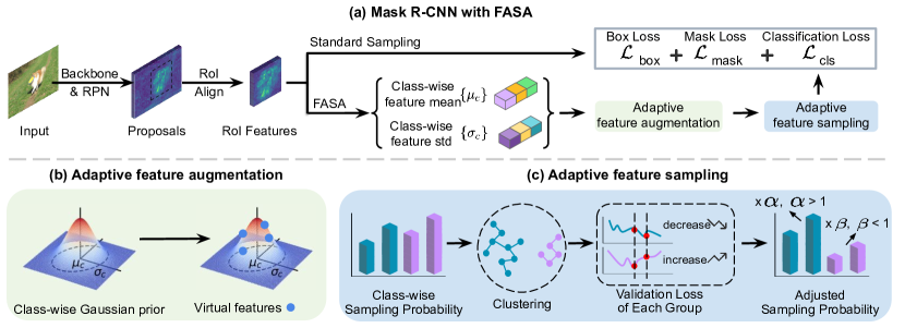
Figure 2: (a) The pipeline of Mask R-CNN combined with the proposed FASA, a standalone module that generates virtual features to augment the classification branch for better performance on long-tailed data. FASA maintains class-wise feature mean and variance online, followed by (b) adaptive feature augmentation and (c) adaptive feature sampling.

In this section, we introduce the proposed Feature Augmentation and Sampling Adaptation (FASA) approach consisting of two components: 1) adaptive Feature Augmentation (FA) that generates virtual features to augment the feature space of all classes (especially for rare classes), 2) adaptive Feature Sampling (FS) that dynamically adjusts the sampling probability of virtual features for each class.

To better illustrate how FASA works for long-tailed instance segmentation, we take the Mask R-CNN [16] framework as our baseline and show an example of combining FASA and the segmentation baseline. The overall pipeline is shown in Fig. 2. Note FASA is a standalone module for feature augmentation, leaving the baseline module unaltered. Therefore, FASA serves as a plug-and-play module and it can combine with and facilitate stronger baselines other than Mask R-CNN. We will show this flexibility in our experiments.

Under the Mask R-CNN framework, the standard multi-task loss is defined for each Region of Interest (RoI):

$$\mathcal{L}=\mathcal{L}_{cls}+\mathcal{L}_{box}+\mathcal{L}_{mask}.$$ (1)

For simplicity, we apply FASA to the classification branch only, which is the most vulnerable branch on long-tailed data as supported in Fig. 1(b). More discussion is provided in the supplementary materials. It is possible to augment other branches using FASA as well. We leave that to future work and expect further improvements.

3.1 Adaptive Feature Augmentation

Mask R-CNN is originally trained on “real” feature embeddings of positive region proposals generated by the Region Proposal Network (RPN). For each class, we aim to augment its real features that are likely scarce (e.g., for rare classes). An ideal FA component should have the following properties: 1) generate diverse virtual features to enrich the feature space of corresponding class, 2) the generated virtual features capture intra-class variations accurately and do not deviate much from the true manifold which hinders learning, 3) adapt to the actual feature distribution that is evolving during training, 4) high efficiency.

To this end, we maintain an online Gaussian prior from previously observed real features, which fulfills the above-mentioned requirements. We found such prior suffices for FA purpose by generating up-to-date and diverse features even when the actual features are not Gaussian. Concretely, for each foreground class $c$ within the current batch, we can calculate the corresponding feature mean $\mu_{c}^{t}\in\mathbb{R}^{d}$ and standard deviation $\sigma_{c}^{t}\in\mathbb{R}^{d}$ which together define a Gaussian feature distribution. Given the noisy nature of $\mu_{c}^{t}$ and $\sigma_{c}^{t}$, we use them to continuously update the more robust estimates $\mu_{c}$ and $\sigma_{c}$ instead, via a momentum mechanism:

$$\mu_{c} \leftarrow(1-m)\cdot=\mu_{c}+m\cdot\mu_{c}^{t},$$ (2)

$$\sigma_{c} \leftarrow(1-m)\cdot\sigma_{c}+m\cdot\sigma_{c}^{t},$$

where $m$ is set to $0.1$ in all experiments. Then according to a Gaussian prior with up-to-date $\mu_{c}$ and $\sigma_{c}$, we generate the class-wise virtual features $\hat{x}_{c}$ by random perturbation under the feature independence assumption:

$$\hat{x}_{c}=\mu_{c}+\sigma_{c}\odot\epsilon,\;\;\;\;\epsilon\sim\mathcal{N}(0,I_{d}).$$ (3)

The feature independence assumption allows for efficient FA, where augmented features are treated as IID random variables. We consider the covariance matrix of the Gaussian to be diagonal, thus largely reduce the complexity from $d^{2}$ to $d$. Such generated virtual features $\{\hat{x}_{c}\}$ will need to be re-sampled (detailed later). Finally, both re-sampled $\{\hat{x}_{c}\}$ and real features $\{x_{c}\}$ (with its own sampling strategy in any baseline method) are sent to compute $\mathcal{L}_{cls}$ in Eq. (1).

3.2 Adaptive Feature Sampling

For a wise use of the generated virtual features for each class, we propose an adaptive Feature Sampling (FS) scheme to effectively avoid under-fitting or over-fitting from FA. The sampling process operates in a relative fashion: if virtual features improve the corresponding class performance, their sampling probabilities get increased, otherwise decreased. Such relative adjustments of virtual feature sampling probabilities cater to the changing needs of FA during training. We can imagine that FA may be useful for rare classes during some training periods, but other training stages may call for decreased amount of FA to avoid over-fitting. By contrast, a static predefined sampling distribution would be independent of training dynamics and thus suboptimal.

Parametric sampling formulation. Note we still need an initial feature sampling distribution so as to adjust it later on. Obviously, we can benefit from a good initialization that avoids initial biased FA and costly adjustments. We choose to initialize the sampling distribution simply based on the inverse class frequency. It favors rare classes with higher sampling probabilities $p_{c}$ and is useful in our class-imbalanced setting with minimal assumption about data distribution. Now we have a predefined skewed sampling distribution at the beginning. Then we dynamically scale the per-class sampling probability $p_{c}$ as follows:

$$p_{c}=s_{c}\cdot\left(\frac{1}{N_{c}}\right)/\sum_{c=1}^{C}\left(\frac{1}{N_{c}}\right),$$ (4)

where $s_{c}$ is the scaling factor to be estimated at each time, and $N_{c}$ denotes the class size of class $c$.

Adaptive sampling scheme. Recall the insight behind adapting the sampling probability $p_{c}$ is that: if FA does improve the performance of class $c$, then we should generate more virtual features and increase $p_{c}$; if we observe worse performance from FA, then $p_{c}$ is probably big enough and we should decrease it to avoid over-fitting with the augmented features. In practice, we use multiplicative adjustments to update $p_{c}$ every epoch. Specifically, we increase $p_{c}$ to $\min(1,p_{c}\cdot\alpha)$ with $\alpha=1.1$, and decrease $p_{c}$ to $\max(0,p_{c}\cdot\beta)$ with $\beta=0.9$.

One can adopt different performance metrics to guide the adjustment of $p_{c}$. Existing adaptive learning systems are either based on the surrogate loss [35] or the more ideal actual evaluation metric [20]. However for large-scale instance segmentation tasks, frequent evaluation of metrics like mAP on large datasets is very expensive. Therefore, we use the classification loss $\mathcal{L}_{cls}$ on validation set to adjust $p_{c}$ for our large-scale segmentation task. For the validation set, we apply Repeat Factor Sampling (RFS) [15] method to balance the class distribution and provide more meaningful losses. The aforementioned setting works reasonably well in our experiments.

Group-wise adaptation. To make our method more robust to different scenarios, we need to address two common challenges in the long-tailed instance segmentation task. First, the per-class loss can be extremely noisy on limited evaluation data, e.g., for rare classes. In this case, both loss and metric cannot serve as reliable performance indicators. Second, the evaluation data may simply not be available for all classes. For example, the validation set of LVIS dataset [15] only has 871 classes out of 1203 from training set. This makes it impossible to evaluate loss for the other 332 classes on validation set.

To solve the aforementioned issues, we propose to cluster all training classes into super-groups. Then we compute the average validation loss of within-group classes, and adjust their feature sampling probabilities together. In other words, we adjust the sampling probabilities by a single scaling factor ($\alpha$ or $\beta$) depending on the average of group-wise loss. By doing so, those classes with missing evaluation data can be safely ignored when computing the loss average, but their sampling probabilities can still be updated along with other classes within the same group. Moreover, the group-wise update is less noisy since it is based on the loss average computed on bigger data (from multiple classes).

For clustering, rather than using predefined heuristics like class size or semantics as in [25, 45], we use the online class-wise feature mean $\mu_{c}$ and standard deviation $\sigma_{c}$. We adopt the density-based [12] clustering algorithm using the following distance based on Fisher’s ratio:

$$d_{ij}=\frac{(\mu_{i}-\mu_{j})^{2}}{\sigma^{2}_{i}+\sigma^{2}_{j}}.$$ (5)

The resulting super-groups are much more adaptive and meaningful than the predefined ones (e.g., rare, common, and frequent class groups), and facilitate better group-wise feature re-sampling. Please refer to the supplementary materials for the visualization of some super-groups of semantically similar classes.

4 Experiments

Table 1: Ablation study of the proposed FASA method on LVIS v1.0 validation set. ‘FA’ denotes adaptive Feature Augmentation, and ‘FS’ denotes adaptive Feature Sampling. The metrics AP, AP${}_{\textrm{r}}$, AP${}_{\textrm{c}}$ and AP${}_{\textrm{f}}$ denote the mask mAP for overall, rare, common and frequent class groups.

FA	FS	AP	AP${}_{\textrm{r}}$	AP${}_{\textrm{c}}$	AP${}_{\textrm{f}}$
✗	✗	20.8	8.0	20.2	27.0
✓	✗	22.3 (+1.5)	12.7 (+5.7)	21.7	26.9
✓	✓	23.7 (+2.9)	17.8 (+9.8)	22.9	27.2

Datasets. Our experiments are conducted on two datasets: LVIS v1.0 [15] with 1203 categories and COCO-LT [42] with 80 categories. Both of them are designed for long-tailed instance segmentation with highly class-imbalanced distribution. We choose LVIS v1.0 dataset over LVIS v0.5 since the former has more labeled data for meaningful evaluations and comparisons. LVIS v1.0 dataset defines three class groups: rare [1, 10), common [10, 100), and frequent [100, -) based on the number of images that contain at least one instance of the corresponding class. Similarly, COCO-LT dataset defines four class groups [1, 20), [20, 400), [400, 8000), [8000, -). We use the standard mean average precision (mAP) as the evaluation metric. Using this metric on different class groups can well characterize the long-tailed class performance. Following [15], we denote the corresponding performance metrics of rare, common and frequent class groups as AP${}_{\textrm{r}}$, AP${}_{\textrm{c}}$ and AP${}_{\textrm{f}}$. Recently, Dave et al. [10] proposed that the mAP metric is sensitive to changes in cross-category ranking, and introduced two complementary metrics AP${}^{\text{Fixed}}$ and AP${}^{\text{Pool}}$. We also report the performance of FASA under the AP${}^{\text{Fixed}}$ and AP${}^{\text{Pool}}$ metrics in the supplementary materials.

Implementation details. Our implementation is based on the MMDetection [6] toolbox. We follow the same experimental setting as in [15, 37] for fair comparison. Please refer to supplementary materials for other details.

4.1 Ablation Study on LVIS

We first perform ablation studies on the large-scale LVIS dataset. We report the validation performance to ablate the core modules of our FASA approach.

Effectiveness of FA and FS. Table 1 verifies the critical roles of our adaptive modules for Feature Augmentation (FA) and Feature Sampling (FS). The baseline (top row) only performs repeat factor sampling [15] for real features, without using any FASA components. Our FA module (second row) significantly improves the performance, both for overall and rare classes. Our adaptive FS further boosts the performance, especially in the rare class groups ($AP_{r}^{m}$ $12.7\%\rightarrow 17.8\%$) with other groups being competitive. The results suggest the effectiveness of both the FA and FS components in improving the training performance.

Table 2: Comparing our FASA with 1) interpolation based methods SMOTE [4] and MoEx [23], 2) copy-and-paste base methods InstaBoost [13], 3) feature augmentation based methods Yin et al. [48], Liu et al. [28], Chu et al. [8] on LVIS v1.0 validation set. The baseline (top row) denotes Mask R-CNN [16] without any augmentation.

Augmentation	AP	AP${}_{\textrm{r}}$	AP${}_{\textrm{c}}$	AP${}_{\textrm{f}}$
✗	20.8	8.0	20.2	27.0
SMOTE [4]	21.5 (+0.7)	10.2 (+2.2)	20.9	27.1
MoEx, CVPR’21 [23]	21.2 (+0.4)	9.2 (+1.2)	20.6	27.1
InstaBoost, CVPR’19 [13]	21.4 (+0.6)	10.3 (+2.3)	20.7	27.2
Yin et al., CVPR’19 [48]	21.6 (+0.8)	11.1 (+3.1)	20.9	27.1
Liu et al., CVPR’20 [28]	21.0 (+0.2)	9.6 (+1.6)	20.1	26.8
Chu et al., ECCV’20 [8]	21.4 (+0.6)	9.7 (+1.7)	21.0	27.0
FASA (ours)	23.7 (+2.9)	17.8 (+9.8)	22.9	27.2

Comparison with other augmentation methods. To further show the simplicity and efficacy of our method, we compare with the classic SMOTE method [4], MoEx [23], InstaBoost [13] and state-of-the-art methods [28, 8, 48] that are specially designed for the long-tailed setting. Since [28, 8, 48] only report results on face recognition and person Re-ID, while no public codes are available, we re-implemented them and optimized their parameters and performance for LVIS (see the supplementary materials for implementation details).

Table 2 shows favorable results of our FASA when compared to others. Our gains are particularly apparent for AP${}_{\textrm{r}}$ and AP${}_{\textrm{c}}$. Since SMOTE [4], MoEx [23] and InstaBoost [13] are not directly designed for long-tailed setting, we verify that our FASA obtains a favorable performance over them. For more related feature augmentation approaches [8, 28, 48], we observe some limitations when transferring them into the instance segmentation task. Liu et al. [28] are based on margin-based face recognition loss such as ArcFace [11] that constrains the margin between each instance and its class anchor. Unfortunately, since the instance segmentation task has to deal with the special background class that no distinct anchor, the margin-based loss does not perform well on LVIS. In contrast, our approach is not restricted by the form of loss function. As for Chu et al. [8], the performance is limited by the small batch size of the instance segmentation task, which does not guarantee the selection of top confusing samples. Both [8] and [48] apply feature transfer from head to tail classes. They use a two-stage training pipeline that requires a pre-trained model to extract features. In contrast, our proposed FA method can be trained end-to-end, much faster than  [8, 48] and only incurs a small extra memory which is constant.

Table 3: Comparison between our adaptive feature sampling strategy and a static one (with fixed scaling factor $s_{c}$ in Eq. (4)).

Sampling Method	AP	AP${}_{\textrm{r}}$	AP${}_{\textrm{c}}$	AP${}_{\textrm{f}}$
Static ($s$ = 1)	21.7	12.2	20.8	27.0
Static ($s$ = 5)	22.3	12.7	21.7	26.9
Static ($s$ = 15)	21.3	12.0	20.2	26.6
Adaptive	23.7	17.8	22.9	27.2

Analysis of adaptive FS. Recall in Eq. (4), our class-wise feature sampling probabilities are adaptively adjusted by the scaling factor $s_{c}$ in an adaptive manner. Table 3 validates our design, showing that sampling is poor with a static sampling strategy. Specifically, we observe that $s_{c}=5$ works best for AP${}_{\textrm{r}}$, but is not optimal for AP${}_{\textrm{f}}$ that needs $s_{c}=1$ instead. On the other hand, our adaptive FS tunes $s_{c}$ online to effectively re-balance the performance across categories.

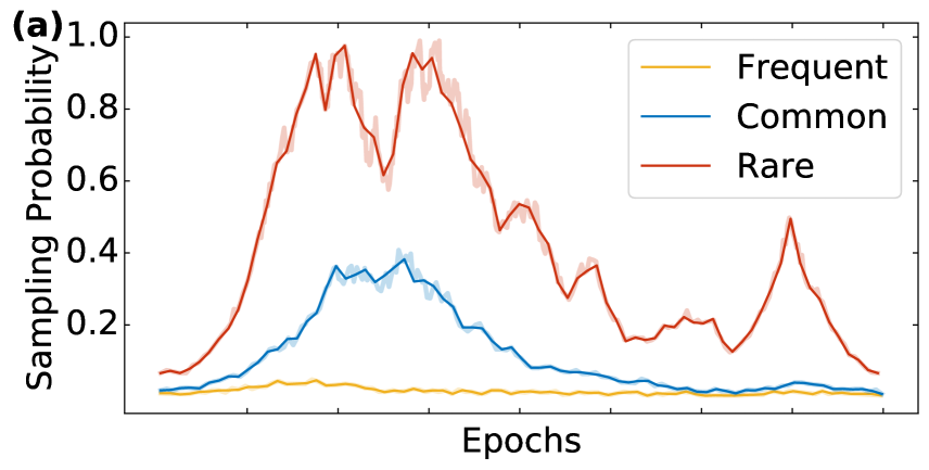
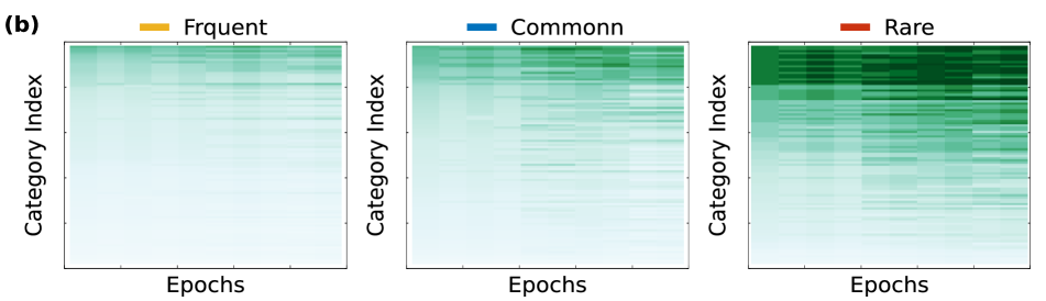
Figure 3: Visualization of the class-wise sampling probabilities during training. (a) We show the average sampling probabilities for the rare/common/frequent class groups. (b) The changing behavior of class-wise sampling probabilities within each group.

Fig. 3(a) depicts how the class-wise sampling probabilities change during training. Overall, the rare classes exhibit high sampling probabilities compared with the common and frequent classes. The rare-class sampling probabilities typically get increased to use more virtual features at the beginning. Then they gradually decrease to avoid over-fitting. Upon convergence, when the learning rate decreases, the sampling probabilities of rare categories see a bump to help with the corresponding classifier ’fine-tuning’. By contrast, the changes of sampling probabilities for the common and frequent classes are smaller. Fig. 3(b) further shows the dynamic changes of sampling probabilities within each class group.

4.2 Comparison with State of the Arts on LVIS

Table 4: Comparing state-of-the-art methods with and without our FASA on the LVIS v1.0 validation dataset. We compare with the Mask R-CNN baseline, and state-of-the-art re-sampling approach Repeat Factor Sampling (RFS) [15], Equalization Loss (EQL) [37], Classifier Re-training (cRT) [21], Balanced Group Softmax (BAGS) [25] and Seesaw Loss [41]. The ‘Uniform’ method indicates random and uniform sample images. These methods are trained under different training schedules (24 or 12+12 epochs) using the public codes. All methods use ResNet-50 [17] as the backbone for fair comparison.

Loss	Sampler	$\#$Epochs	FASA	AP	AP${}_{\textrm{r}}$	AP${}_{\textrm{c}}$	AP${}_{\textrm{f}}$
Softmax CE	Uniform	24	✗	19.3	1.2	17.4	29.3
			✓	22.6 (+3.3)	10.2 (+9.0)	21.6	29.2
	RFS, CVPR’19 [15]	24	✗	22.8	12.9	21.6	28.3
			✓	24.1 (+1.3)	17.3 (+4.4)	22.9	28.5
EQL, CVPR’20 [37]	Uniform	24	✗	22.1	5.1	22.4	29.3
			✓	24.4 (+2.3)	15.4 (+10.3)	23.5	29.4
cRT, ICLR’20 [21]	Uniform / RFS, CVPR’19 [15]	12+12	✗	22.4	12.2	20.4	29.1
			✓	23.6 (+1.2)	15.1 (+2.9)	22.0	29.1
BAGS’ CVPR’20 [25]	Uniform / RFS, CVPR’19 [15]	12+12	✗	22.8	12.4	22.2	28.3
			✓	24.0 (+1.2)	15.2 (+2.8)	23.4	28.3
Seesaw, CVPR’21 [41]	RFS, CVPR’19 [15]	24	✗	26.4	19.6	26.1	29.8
			✓	27.5 (+1.1)	21.0 (+1.4)	27.5	30.1

Table 5: Comparison state-of-the-art methods with and without FASA, using large backbones (ResNet-101 [17], ResNeXt-101-32x8d [47]) and advanced Cascade Mask R-CNN [2] framework.

Method	Loss	Sampler	Backbone	FASA	AP	AP${}_{\textrm{r}}$	AP${}_{\textrm{c}}$	AP${}_{\textrm{f}}$
Mask R-CNN, ICCV’17 [16]	Softmax CE	RFS, CVPR’19 [15]	R101	✗	24.4	13.2	24.7	30.3
				✓	26.3 (+1.9)	19.1 (+5.9)	25.4	30.6
Mask R-CNN, ICCV’17 [16]	Softmax CE	RFS, CVPR’19 [15]	X101	✗	26.1	16.1	24.9	32.0
				✓	27.7 (+1.6)	20.7 (+4.6)	26.6	32.0
Cascade Mask R-CNN, TPAMI’19 [2]	Softmax CE	RFS, CVPR’19 [15]	R101	✗	25.4	13.7	24.8	31.4
				✓	27.7 (+2.3)	19.8 (+5.9)	27.3	31.6
Cascade Mask R-CNN, TPAMI’19 [2]	Seesaw, CVPR’21 [41]	RFS, CVPR’19 [15]	R101	✗	30.1	21.4	30.0	33.9
				✓	31.5 (+1.4)	24.1 (+2.7)	31.9	34.0

In this section, we evaluate the full FASA method against state-of-the-art methods on the LVIS v1.0 dataset. We consider the following representative methods: 1) Repeat Factor Sampling (RFS) [15] is an image-level data re-sampling technique. We use the same repeat factor $1e-3$ as proposed in the original paper. 2) Equalization Loss (EQL) [37] is a loss re-weighting method that aims to ignore the harmful gradients from rare classes. 3) Classifier Re-training (cRT) [21] first uses random sampling for feature representation learning, and then re-trains the classifier with repeat factor sampling. 4) Balanced Group Softmax (BAGS) [25] first performs class grouping and then makes the classification loss relatively balanced across those class groups. Grouping simply relies on the class sizes that are independent of training dynamics and suboptimal. 5) Seesaw Loss [41] balances ratio of cumulative gradients for the positive samples and negative samples of different categories.

Comparing using Mask R-CNN baseline. The aforementioned methods have shown solid improvements when combined with the Mask R-CNN baseline. Here we conduct a more comprehensive comparison with even stronger versions of these methods under different training schedules. Specifically, we experimented with the default 12 and 24 epochs schedules [6], as well as the decoupled two-stage training schedule [21, 25]. In the first stage, we train the model for 12 epochs with standard random data sampling and cross-entropy loss. Then in the second stage, we fine-tune for 12 epochs using those advanced re-sampling or re-weight approaches, such as RFS and BAGS. We refer to this schedule as ‘12+12’. We compare with all of these methods by plugging in our FASA module and comparing the performance difference.

Table 4 summarizes the comparison results. Specifically, we repeat each experiment three times with different random seeds and report the mean value of results. When we combine our FASA with vanilla Mask R-CNN, we observe huge 3.3% gains in the overall metric AP. Our benefits are particularly evident in the rare class performance AP${}_{\textrm{r}}$, with gains of 9.0%. This validates FASA’s superior ability to deal with long-tailed tasks. We also verify that the benefits of FASA remain consistent over multiple runs. When combined with stronger methods (RFS/EQL/cRT/BAGS/Seesaw) or training schedules, FASA can still obtain consistent improvements in overall AP, where the rare-class improvements in AP${}_{\textrm{r}}$ dominate. Such gains come without compromising the common- and frequent-class metrics AP${}_{\textrm{c}}$ and AP${}_{\textrm{f}}$, where FASA performs better or remains on par.

Long training schedules and large backbones. FASA works well even with large backbones (ResNet 101 [17], ResNeXt 101-32-8d [47]) and advanced instance segmentation framework Cascade Mask R-CNN [2]. As shown in Table 5, the benefits of FASA still hold under different settings. On the validation set, FASA improves the performance of Mask R-CNN baseline (ResNet-101 backbone) by a large margin. We observe improvements in overall AP and rare-class AP${}_{\textrm{r}}$ by 1.9% and 5.9% respectively. For the stronger ResNeXt101 backbone, we observe similar trend. FASA significantly improves the rare class performance AP${}_{\textrm{r}}$ by 4.6%. For Cascade Mask R-CNN [2] framework and Seesaw loss [41], FASA offers consistent performance boost in rare classes while remaining strong on both common and frequent classes.

Analyzing classifier weight norm. As discussed in [21, 25], the weight norm of a classifier is correlated with the imbalanced learning performance, with the weight norms of tail classes often being much smaller on long-tailed data. Fig. 4 visualizes the weight norm of classifiers trained with and without FASA. It can be seen that FASA leads to more balanced class distributions of weight norms than Cross-Entropy baseline and Seesaw Loss [41]. This partially explains why FASA greatly improves the rare-class performance of these methods.

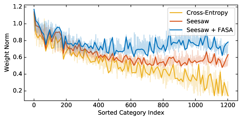
Figure 4: Comparison of the classifier weight norm of Cross-Entropy and Seesaw Loss [41] (with and without FASA). Our FASA leads to a more class-balanced weight norm distribution.

4.3 Evaluation on COCO-LT

We evaluated FASA on COCO-LT [42] dataset to examine the generalizability of our approach. For a fair comparison, we follow the same experiment setting as SimCal [42]. There are two main differences compared to the implementation details we described in the LVIS dataset: (1) Single-scale training is used. We set the input image’s short side to 800 pixels and do not use multi-scale jittering. (2) The bounding box head and mask head are class agnostic.

Table 6 summarizes the results. The top row shows results of the Mask R-CNN [16] with ResNet50 [17] backbone and FPN [26] neck. The second row shows results obtained by the previous state-of-the-art method SimCal [42], which involves classification calibration training and then dual head inference. The third row shows results of the Mask R-CNN baseline augmented with our FASA. Note how FASA improves the performance of Mask R-CNN considerably, especially for those rare classes ($\mathrm{AP}^{\mathrm{m}}_{\mathrm{1}}$ and $\mathrm{AP}^{\mathrm{m}}_{\mathrm{2}}$). Overall, FASA performs better than SimCal [42] without any form of decoupled training.

Table 6: Results on COCO-LT [42] minival set. $\mathrm{AP}^{\mathrm{m}}$ and $\mathrm{AP}^{\mathrm{b}}$ denote the Mask mAP and Bbox mAP, respectively. $\mathrm{AP}^{\mathrm{m}}_{\mathrm{1}}$, $\mathrm{AP}^{\mathrm{m}}_{\mathrm{2}}$, $\mathrm{AP}^{\mathrm{m}}_{\mathrm{3}}$, $\mathrm{AP}^{\mathrm{m}}_{\mathrm{4}}$ refer to bin of $[1,20)$, $[20,400)$, $[400,8000)$, $[8000,-)$ training instances.

Method	$\mathrm{AP}^{\mathrm{m}}$	$\mathrm{AP}^{\mathrm{m}}_{\mathrm{1}}$	$\mathrm{AP}^{\mathrm{m}}_{\mathrm{2}}$	$\mathrm{AP}^{\mathrm{m}}_{\mathrm{3}}$	$\mathrm{AP}^{\mathrm{m}}_{\mathrm{4}}$	$\mathrm{AP}^{\mathrm{b}}$
Mask R-CNN	18.7	0.0	8.2	24.4	26.0	21.4
SimCal [42]	21.8	15.0	16.2	24.3	26.0	24.6
FASA (Ours)	23.4	13.5	19.0	25.2	27.5	26.0

4.4 Evaluation on CIFAR-LT-100

Table 7: Comparison of classification accuracy on CIFAR-LT-100 [3] dataset with imbalance ratio 100. $\dagger$ denotes that the results are copied from [22].

Backnone	Method	Augmentation	Accuracy ($\%$)
ResNet 32	LDAM [3] $\dagger$	✗	42.0 $\pm$ 0.09
	LDAM [3]	M2M [22]	43.5 $\pm$ 0.22
	LDAM [3]	FASA(Ours)	43.7 $\pm$ 0.25
	De-confound-TDE [38]	✗	44.1
	De-confound-TDE [38]	FASA (Ours)	45.2 $\pm$ 0.16
ResNet 34	Cross entropy	Chu et al. [8]	48.5
	Cross entropy	FASA(Ours)	49.1 $\pm$ 0.23

To demonstrate the generalizability of FASA in other domains, we further apply FASA on the long-tailed image classification task. We follow [3] to conduct experiments on the long-tailed CIFAR-100 dataset with a substantial imbalance ratio of $\rho=100$ (the ratio between sample sizes of the most frequent and least frequent class, $\rho=\max_{i}\{N_{i}\}/\min_{i}\{N_{i}\}$). We train for 200 epochs and use the top-1 accuracy as the evaluation metric. We compare FASA with two state-of-the-art feature-level augmentation approaches M2M [22] and Chu et al. [8]. When comparing with M2M [22], we use LDAM [3] loss as the baseline for a fair comparison. We use the same backbones of [22, 8] to experiment under the same settings.

From Table 7, we observe that our FASA brings 1.7$\%$ accuracy improvement over the LDAM [3] baseline and is comparable with M2M [22]. When applied to the stronger baseline De-confound-TDE [38], FASA’s benefits still hold. FASA is also better performing than Chu et al. [8] with the cross entropy loss. Other than that, our FASA is more time-efficient than M2M [22] and Chu et al. [8] because they need extra time for classifier pre-training while FASA can be applied online.

5 Conclusion

We have presented a simple yet effective method, Feature Augmentation and Sampling Adaptive (FASA), to address the class imbalance issue in the long-tailed instance segmentation task. FASA generates virtual features on the fly to provide more positive samples for rare categories, and leverages a loss-guided adaptive sampling scheme to avoid over-fitting. FASA achieves consistent gains on the Mask R-CNN baseline under different backbones, learning schedules, data samplers and loss functions, with minimal impact to the training efficiency. It shows large gains for rare classes without compromising the performance for common and frequent classes. Notably, as an orthogonal component, it improves other more recent methods such as RFS, EQL, cRT, BAGS and Seesaw. Compelling results are shown on two challenging instance segmentation datasets, LVIS v1.0 and COCO-LT, as well as an imbalanced image classification benchmark, CIFAR-LT-100.

Acknowledgements. This study is supported under the RIE2020 Industry Alignment Fund – Industry Collaboration Projects (IAF- ICP) Funding Initiative, as well as cash and in-kind contribution from the industry partner(s).

Appendix

In the supplementary materials, we discuss the ablation studies and implementation details that are not elaborated in the main paper. Section A highlights our FASA largely reduces the classification error. Section B analyzes some ablation studies of the adaptive feature sampling module. Section C validates the memory- and time-efficiency of FASA. Section D presents the clustering results used in the feature space. Section E provides the performance of FASA under the recently proposed AP${}^{\text{Fixed}}$ and AP${}^{\text{Pool}}$ metrics [10]. Section F reports our implementation details of feature augmentation methods. Section G compares FASA with another instance-level re-sampling based approach NMS re-sampling [45]. Section H shows the visualization result of FASA.

Appendix A Error Analysis of Long-Tailed Instance Segmentation: Classification Error Dominates

Table 8: Error analysis of Mask R-CNN [16] with and without FASA. We use the TIDE [1] toolbox and report the six error types (%) on LVIS v1.0 validation set: classification error ($\mathrm{E}_{\mathrm{cls}}$), location error ($\mathrm{E}_{\mathrm{loc}}$), both classification and location error ($\mathrm{E}_{\mathrm{both}}$), duplicate detection error ($\mathrm{E}_{\mathrm{dupe}}$), background error $\mathrm{E}_{\mathrm{bkg}}$ and missed ground truth error ($\mathrm{E}_{\mathrm{miss}}$). We observe the dominance of $\mathrm{E}_{\mathrm{cls}}$ for Mask R-CNN, and hence apply FASA only to the classification branch of Mask R-CNN at minimum cost. This leads to big improvements in $\mathrm{E}_{\mathrm{cls}}$ already. We expect more gains in $\mathrm{E}_{\mathrm{cls}}$ and other error metrics by augmenting other branches of Mask R-CNN if given more computational budget.

Method	$\mathrm{E}_{\mathrm{cls}}$	$\mathrm{E}_{\mathrm{loc}}$	$\mathrm{E}_{\mathrm{both}}$	$\mathrm{E}_{\mathrm{dupe}}$	$\mathrm{E}_{\mathrm{bkg}}$	$\mathrm{E}_{\mathrm{miss}}$
Mask R-CNN	25.10	6.71	0.59	0.36	3.17	7.15
+ FASA	20.74	6.80	0.50	0.41	3.48	7.29
$\Delta$	-4.36	+0.09	-0.09	+0.05	+0.29	+0.14

In the main paper, we apply FASA only to the classification branch of Mask R-CNN. But why the choice? How does this simple mechanism impact performances of other branches like detection? To answer such questions, we need a detailed error analysis other than the default, single metric mean-average precision (mAP). We use the recent TIDE [1] toolbox to report six error metrics for long-tailed instance segmentation.

Table 8 outlines the six error metrics on large-scale LVIS dataset. We see that for the Mask R-CNN baseline [16], classification error is the main bottleneck for long-tailed instance segmentation when compared to other error types, e.g., localization error. This explains our use of FASA to the classification branch of Mask R-CNN. Obviously, augmenting classification branch only will not incur a high cost. Performance-wise, we do see a significant reduction in classification error (from $25.10$% to $20.74$%) without deteriorating other errors much. With more budget, one could apply FASA to augment other branches of Mask R-CNN with the hope of more gains in all error metrics.

Appendix B Ablation on Adaptive Feature Sampling

B.1 Initial Feature Sampling Probabilities

To initialize our adaptive virtual feature sampling process, we assigned class-wise sampling probabilities based on inverse class frequency. This scheme favors rare-class feature augmentation at the beginning, and does not rely on too many assumptions about skewed data distribution. Another sampling scheme that has minimal assumption of data distribution is based on uniform class distribution.

Table 9 compares the two schemes empirically. We see that both the uniform initialization and the inverse class frequency initialization boost the performance compared with the no augmentation baseline. Overall, the inverse class frequency initialization approach achieves better overall mask mAP. The AP${}_{\textrm{r}}$ and AP${}_{\textrm{f}}$ results of uniform initialization are slightly worse than initialization based on inverse class frequency. So we use the initialization based on inverse class frequency by default for its effectiveness and simplicity.

Table 9: Comparing different initialization schemes of our virtual feature sampling probabilities. AP, AP${}_{\textrm{r}}$, AP${}_{\textrm{c}}$ and AP${}_{\textrm{f}}$ refer to the mask mAP metrics (%) for overall, rare, common and frequent class groups. The symbol ‘FS’ denotes to our adaptive Feature Sampling module.

FS	Initial sampling probability	AP	AP${}_{\textrm{r}}$	AP${}_{\textrm{c}}$	AP${}_{\textrm{f}}$
✗	✗	22.3	12.7	21.7	26.9
✓	Uniform distribution	23.2	15.1	23.4	26.6
✓	Inverse class frequency	23.7	17.8	22.9	27.2

B.2 Performance Metric for Sampling Adaptation

In the main paper, we propose a virtual feature sampling approach that is adapted to the validation loss rather than validation metric. This is to avoid the large computational cost from frequent metric evaluation on large-scale dataset. Concretely, evaluating the validation metric of mAP on the dataset takes nearly 45 minutes, which is very expensive if we were to conduct it in each epoch. To test how much we can gain from adapting to the true performance metric, we compare the use of the two supervisory signals on a smaller task. We choose the long-tailed image classification task on CIFAR-100-LT [3], a much smaller dataset than LVIS. Evaluating per-class accuracy is as efficient as evaluating the loss on CIFAR-100-LT validation set. Table 10 shows a marginal improvement from using the performance metric, which when translated to large-scale dataset, may not be worth the large cost for metric evaluation.

Table 10: Comparing the use of different performance metrics (validation loss vs. metric) for adaptive feature sampling on CIFAR-100-LT [3] dataset. The average and standard deviation of classification accuracy are from 3 runs.

Perf. measurement	Accuracy ($\%$)
Validation loss	43.7 $\pm$ 0.25
Validation metric	43.9 $\pm$ 0.38

B.3 Group-wise vs. Class-wise Adaptation

By default, we adjust the feature sampling probability for each class group rather than each class. One of the reasons is that some classes may be missing for performance evaluation, e.g., on LVIS validation set. This makes it impossible for loss-adapted sampling probability adjustment for every class. But what if all classes are available for evaluation, appearing on both training and validation sets?

We again test on the CIFAR-100-LT [3] dataset that meets the requirement. In this case, class grouping is not a must anymore, and our goal is to see if group-wise sampling adaptation still holds its benefits over class-wise sampling adaptation. Table 11 gives a positive answer. We observe that group-wise sampling adaptation performs better and has a lower variance since it relies on the stabler group-wise loss average rather than the noisy per-class loss.

Table 11: Comparing the group-wise and class-wise feature sampling adaptation on CIFAR-100-LT [3] dataset. The average and standard deviation of classification accuracy are from 3 runs.

Sampling adaptation	Accuracy ($\%$)
Group-wise	43.7 $\pm$ 0.25
Class-wise	43.3 $\pm$ 0.85

Table 12: Comparison of training memory $\mathrm{M}_{\mathrm{train}}$ and training time $\mathrm{T}_{\mathrm{train}}$ required, with and without FASA on LVIS v1.0.

Method	FASA	$\mathrm{M}_{\mathrm{train}}$ (GB)	$\mathrm{T}_{\mathrm{train}}$ (s/iter)
Mask R-CNN + RFS	✗	11.1	0.768 $\pm$ 0.04
	✓	12.4	0.792 $\pm$ 0.05

Appendix C Speed Analysis

Table 12 further validates the memory- and time-efficiency of our FASA approach. We see that FASA adds only a small amount of memory, which is used to maintain the online feature mean and variance of observed training samples. Thus the extra memory is constant and dependent only on the feature dimension. FASA is also found to incur a very small time cost.

Appendix D Visualizing Class Grouping Results

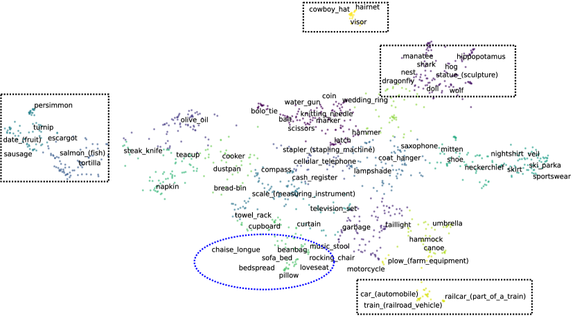
Figure 5: t-SNE [32] visualization of class groups. In the black dashed boxes, classes are often semantically related or visually similar. In the blue ellipse, we find classes that exhibit strong co-occurrence, e.g., between ‘pillow’ and ‘bedspread’.

Recall our feature sampling probabilities are adjusted in a group-wise manner. The class groups are formed by the Mean-shift [7] clustering algorithm. Figure 5 presents some clustering results, where visually similar or semantically related classes stay close in the feature space (e.g., “hairnet” and “visor”). In addition, the co-occurrent classes also tend to stay close (e.g., “pillow” and “loveseat”). Intuitively, related classes are better suited to have their sampling probabilities adjusted together.

Appendix E Evaluation with AP${}^{\text{Fixed}}$ and AP${}^{\text{Pool}}$

The mean average precision metric (denotes as AP${}^{\text{Old}}$ in the following) is the default evaluation metric for the instance segmentation task [27, 15]. Recently, Dave et al. [10] argued that the AP${}^{\text{Old}}$ metric is sensitive to changes in cross-category ranking, and introduced two complementary metrics AP${}^{\text{Fixed}}$ and AP${}^{\text{Pool}}$ to replace AP${}^{\text{Old}}$ for LVIS [15] dataset. Dave et al. [10] found that some methods improve AP${}^{\text{Old}}$ but have less impact on AP${}^{\text{Fixed}}$ and AP${}^{\text{Pool}}$. The AP${}^{\text{Old}}$ metric limits the maximum detection results per image, resulting in cross-category competition. To address this issue, the AP${}^{\text{Fixed}}$ metric limits the maximum detection results per class on the dataset instead. To highlight the score calibration property, Dave et al. [10] also proposed AP${}^{\text{Pool}}$ metric that is class-agnostic and evaluates detection results across all categories together. Since AP${}^{\text{Pool}}$ is class-agnostic, the evaluation is influenced more heavily by frequent classes rather than rare classes.

We provide the experimental results of FASA under the AP${}^{\text{Fixed}}$ and AP${}^{\text{Pool}}$ in Table 13. We observe that FASA consistently boosts the performance under AP${}^{\text{Fixed}}$ and AP${}^{\text{Pool}}$, especially for the rare categories. For AP${}^{\text{Fixed}}$, FASA improves overall AP and rare-class AP${}_{\textrm{r}}$ by 1.1$\%$ / 1.7$\%$ respectively for Mask R-CNN and 1.3$\%$ / 2.4$\%$ for Cascade Mask R-CNN. For AP${}^{\text{Pool}}$, FASA still obtains 2.9$\%$ gains in AP${}_{\textrm{r}}$ for Mask R-CNN and 2.0$\%$ for Cascade Mask R-CNN. Since AP${}^{\text{Pool}}$ is mainly affected by the frequent class, the overall AP improvements are small. The AP${}^{\text{Fixed}}$ and AP${}^{\text{Pool}}$ results also demonstrate that FASA largely improves the performance of rare classes without compromising the common classes and frequent classes.

Table 13: Results of Cascade Mask R-CNN [2] with and without FASA under the recently proposed AP${}^{\text{Fixed}}$ and AP${}^{\text{Pool}}$ metric [10]. We report the results on the LVIS [15] validation set. AP, AP${}_{\textrm{r}}$, AP${}_{\textrm{c}}$ and AP${}_{\textrm{f}}$ refer to the mask mAP metrics (%) for overall, rare, common and frequent class groups. The symbol AP${}^{\text{Old}}$ refers to the standard mean average precision (mAP) metric. We observe FASA offers consistent performance boost under the AP${}^{\text{Fixed}}$ and AP${}^{\text{Pool}}$, especially for the rare categories. All the models use the ResNet-101 [17] backbone and Repeat Factor Sampling (RFS) [15].

		AP${}^{\text{Fixed}}$				AP${}^{\text{Pool}}$
Method	FASA	AP	AP${}_{\textrm{r}}$	AP${}_{\textrm{c}}$	AP${}_{\textrm{f}}$	AP	AP${}_{\textrm{r}}$	AP${}_{\textrm{c}}$	AP${}_{\textrm{f}}$
Mask R-CNN [16]	✗	27.1	20.3	26.9	30.3	27.2	9.0	22.5	27.5
	✓	28.2 (+1.1)	22.0 (+1.7)	28.3	30.9	27.4 (+0.2)	11.9 (+2.9)	23.0	27.8
Cascade Mask R-CNN [2]	✗	28.7	22.2	28.3	32.0	28.9	10.4	24.2	29.4
	✓	30.0 (+1.3)	24.6 (+2.4)	29.8	32.4	29.2 (+0.3)	12.4 (+2.0)	25.0	29.6

Appendix F Implementation Details

Our implementation is based on the Mask R-CNN [16] backbone, which is the ImageNet pre-trained ResNet-50 [17] with a FPN [26] neck and a box head with two sibling fully connected layers for RoI classification and regression. We apply random horizontal image flipping and multi-scale jittering with the smaller image sizes (640, 672, 704, 736, 768, 800) in all experiments. All models are trained with standard SGD on 8 NVIDIA V100 GPUs. We follow the default settings in MMDetection [6] to set other hyper-parameters such as learning rates and training schedules.

Here we also describe the implementation details of the feature augmentation methods listed in Table 2 of the main paper. We detail the hyper-parameters of these approaches and our searched optimal choices in Table 14.

Table 14: Parameters tuned for the feature augmentation methods in Table 2 of the main paper.

Method	Param	Description	Value
MoEx, CVPR’21 [23]	$p$	MoEx probability	1.0
	$\epsilon$	Epsilon constant for standard deviation	$1e^{-5}$
Liu et al., CVPR’20 [28]	$s$	Scaling factor	20
	$m_{a}$	Angular margin	0.1
Chu et al., ECCV’20 [8]	$\mathcal{T}_{s}$	Threshold to extract the class-specific features	0.3
	$\mathcal{T}_{g}$	Threshold to extract the class-generic features	0.6
Yin et al., CVPR’19 [48]	$\alpha_{\text{recon}}$	Coefficient of the reconstruction loss	0.5
	$\alpha_{\text{reg}}$	Coefficient of the regularization loss	0.25

SMOTE [4]. The SMOTE algorithm interpolates neighboring features (i.e., feature embeddings of region proposals) in the feature space. Specifically, for given features $x_{i}$, we consider the $k=5$ nearest neighbours $\{x_{j}\}$ based on cosine feature distance. Then we interpolate new features as:

$$\hat{x}=\lambda\cdot x_{i}+(1-\lambda)\cdot x_{j},$$ (6)

where $\lambda$ is a random value in $(0,1]$.

MoEx [23]. Similar to SMOTE [4], the MoEx is also an interpolation-based augmentation method. As MoEx was developed for the image classification task, we transfer it to the instance segmentation task with the following modification: 1) we applied MoEx augmentation in the classifier of the Mask R-CNN [16] framework, 2) we searched the optimal value of parameters on the LVIS dataset and the results are shown in Table 14.

InstaBoost [13]. InstaBoost is an adaptive copy-and-paste FA method based on a location probability map. Since InstaBoost was already developed for the instance segmentation task, we use its default hyper-parameters.

Liu et al. [28]. Liu et al. [28] propose to transfer the angular distribution of face recognition loss such as CosFace [40] or ArcFace [11]. We select ArcFace for re-implementation:

$$L=-\frac{1}{N}\sum_{n=1}^{N}\log\frac{e^{s\left(\cos\left(\theta_{y}+\alpha_{y}+m_{a}\right)\right)}}{e^{s\left(\cos\left(\theta_{y}+\alpha_{y}+m_{a}\right)\right)}+\sum_{j\neq y}^{C}e^{s\left(\cos\left(\theta_{j}+\alpha_{y}\right)\right)}}$$ (7)

The symbol $\theta_{y}$ refers to the angle between the input feature and the weight of the classifier. The symbol $\alpha_{y}$ means the extra angular that transfers from head class to tail class. As shown in Eq (7), two parameters are involved: the symbol $s$ means the scaling factor applied to logit, and the symbol $m_{a}$ refers to the angular margin. We tune these two parameters and show the results in Table 14.

We observed that since the instance segmentation task has to deal with the special background class, the margin-based ArcFace loss is unfortunately very sensitive to hyper-parameter choices of $m_{a}$. So margin-based augmentation [28] does not perform well on LVIS. Different from Liu et al. [28], our FASA is not limited to the form of loss functions.

Chu et al. [8]. Chu et al. [8] mixed the class-specific features of each class and the corresponding class-generic features of ‘confusing’ classes to synthesize new data samples. The definitions of ‘class-generic’ and ‘class-specific’ are based on the threshold masking of class activation map (CAM) [53]. For each real sample in the tail class, the authors sample $N_{a}$ images from its $N_{f}$ confusing classes.

During the re-implementation, we found that the difference in batch size between the classification and instance segmentation tasks limited the performance of Chu et al. [8] when transferred to the instance segmentation task. The classification task has a large batch size (e.g., 128) that can meet the demand of picking confusing categories (e.g., $N_{a}=N_{f}=3$). However, instance segmentation models are limited by small batch size (e.g., 2) and there is no guarantee that the top confusing categories will appear in the same batch. Compared with Chu et al. [8], our FASA builds feature banks for each category to cache the features of the previous batch, thus getting rid of the small batch limitation.

Yin et al. [48]. Yin et al. [48] is a feature augmentation method designed for the face recognition task. A total of three loss functions are included: face classification loss $\mathcal{L}_{sfmx}$, reconstruction loss $\mathcal{L}_{\text{recon}}$ and regularization loss $\mathcal{L}_{\text{reg}}$. The reconstruction loss $\mathcal{L}_{\text{recon}}$ is critical to train the discriminative feature encoder and decoder. To transfer into the instance segmentation task, we apply the reconstruction loss to the feature embedding of each positive region proposal. Besides, Yin et al. [48] need a two-stage training pipeline. In the first stage, the authors fix the backbone and generate new feature samples to train the classifier. In the second stage, the authors fix the classifier and update the other components. Such a two-stage approach introduces additional training time cost. Compared to Yin et al. [48], our FASA leverages end-to-end training and therefore more efficient.

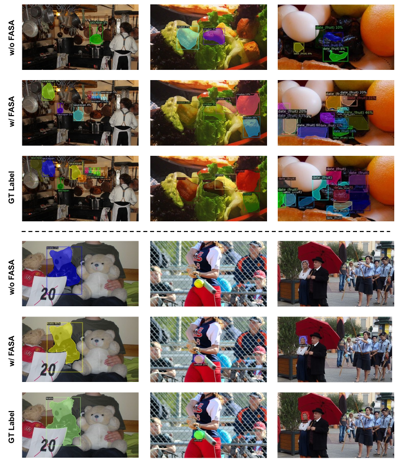
Figure 6: Prediction results of Mask R-CNN framework without and with FASA on the LVIS v1.0 validation set. We select six rare classes ‘saucepan’, ‘crouton’, ‘date (fruit)’, ‘koala’, ‘softball’ and ‘bonnet’ to visualize. We observe that with the help of FASA, Mask R-CNN exhibits more correct classification results than the baseline.

Appendix G Comparison with NMS Re-sampling [45]

NMS Re-sampling [45] is proposed to adjusting the NMS threshold for different categories during the training. Specifically, the NMS thresholds for the frequent/common/rare categories are set as {0.7, 0.8, 0.9} with the increasing trend. Such a mechanism is beneficial to preserve more region proposals from the rare classes and suppress the number of proposals from frequent classes.

Table 15: Comparing our FASA with NMS Re-sampling [45] on LVIS v1.0 validation set. The symbol ‘NR’ denotes the NMS Resampling approach. AP, AP${}_{\textrm{r}}$, AP${}_{\textrm{c}}$ and AP${}_{\textrm{f}}$ refer to the mask mAP metrics (%) for overall, rare, common and frequent class groups.

NR	FASA	AP	AP${}_{\textrm{r}}$	AP${}_{\textrm{c}}$	AP${}_{\textrm{f}}$
✗	✗	19.3	1.2	17.4	29.3
✗	✓	22.6	10.2	21.6	29.2
✓	✗	21.7	8.6	20.4	29.0
✓	✓	22.9	11.1	21.8	29.2

We compare the FASA with NMS Re-sampling in Table 15. The first line refers to the Mask R-CNN [16] baseline without any re-sampling or augmentation method. From the second and the third line, we see that both FASA and NMS Re-sampling achieve better performance than the baseline method. FASA performs slightly better than NMS Re-sampling, especially for the rare classes. We believe such a performance gap is due to NMS Re-Sampling is mainly in adjusting the sampling weights of the current data samples, while FASA can further generate new virtual samplers. Also, the bottom results demonstrate that FASA as an orthogonal module can combine with NMS Re-sampling to further boost the performance.

Appendix H Result Visualization

To better interpret the result, we show the segmentation results of the selected rare classes in Figure 6. We observe that without FASA, the prediction scores for rare classes are small or even missed. On the contrary, with the help of our FASA, the classification results of the rare classes become accurate.

References

- [1] Daniel Bolya, Sean Foley, James Hays, and Judy Hoffman. TIDE: A general toolbox for identifying object detection errors. In ECCV, 2020.
- [2] Zhaowei Cai and Nuno Vasconcelos. Cascade R-CNN: High quality object detection and instance segmentation. TPAMI, 2019.
- [3] Kaidi Cao, Colin Wei, Adrien Gaidon, Nikos Arechiga, and Tengyu Ma. Learning imbalanced datasets with label-distribution-aware margin loss. In NIPS, 2019.
- [4] Nitesh V Chawla, Kevin W Bowyer, Lawrence O Hall, and W Philip Kegelmeyer. SMOTE: Synthetic minority over-sampling technique. JAIR, 16:321–357, 2002.
- [5] Kai Chen, Jiangmiao Pang, Jiaqi Wang, Yu Xiong, Xiaoxiao Li, Shuyang Sun, Wansen Feng, Ziwei Liu, Jianping Shi, Wanli Ouyang, et al. Hybrid task cascade for instance segmentation. In CVPR, 2019.
- [6] Kai Chen, Jiaqi Wang, Jiangmiao Pang, Yuhang Cao, Yu Xiong, Xiaoxiao Li, Shuyang Sun, Wansen Feng, Ziwei Liu, Jiarui Xu, Zheng Zhang, Dazhi Cheng, Chenchen Zhu, Tianheng Cheng, Qijie Zhao, Buyu Li, Xin Lu, Rui Zhu, Yue Wu, Jifeng Dai, Jingdong Wang, Jianping Shi, Wanli Ouyang, Chen Change Loy, and Dahua Lin. MMDetection: Open MMLab detection toolbox and benchmark. arXiv preprint:1906.07155, 2019.
- [7] Yizong Cheng. Mean shift, mode seeking, and clustering. TPAMI, 17(8):790–799, 1995.
- [8] Peng Chu, Xiao Bian, Shaopeng Liu, and Haibin Ling. Feature space augmentation for long-tailed data. In ECCV, 2020.
- [9] Yin Cui, Menglin Jia, Tsung-Yi Lin, Yang Song, and Serge Belongie. Class-balanced loss based on effective number of samples. In CVPR, 2019.
- [10] Achal Dave, Piotr Dollár, Deva Ramanan, Alexander Kirillov, and Ross Girshick. Evaluating large-vocabulary object detectors: The devil is in the details. arXiv preprint arXiv:2102.01066, 2021.
- [11] Jiankang Deng, Jia Guo, Niannan Xue, and Stefanos Zafeiriou. ArcFace: Additive angular margin loss for deep face recognition. In CVPR, pages 4690–4699, 2019.
- [12] Martin Ester, Hans-Peter Kriegel, Jörg Sander, Xiaowei Xu, et al. A density-based algorithm for discovering clusters in large spatial databases with noise. In KDD, volume 96, pages 226–231, 1996.
- [13] Hao-Shu Fang, Jianhua Sun, Runzhong Wang, Minghao Gou, Yong-Lu Li, and Cewu Lu. Instaboost: Boosting instance segmentation via probability map guided copy-pasting. In CVPR, pages 682–691, 2019.
- [14] Golnaz Ghiasi, Yin Cui, Aravind Srinivas, Rui Qian, Tsung-Yi Lin, Ekin D Cubuk, Quoc V Le, and Barret Zoph. Simple copy-paste is a strong data augmentation method for instance segmentation. In CVPR, 2021.
- [15] Agrim Gupta, Piotr Dollar, and Ross Girshick. LVIS: A dataset for large vocabulary instance segmentation. In CVPR, 2019.
- [16] Kaiming He, Georgia Gkioxari, Piotr Dollár, and Ross Girshick. Mask R-CNN. In ICCV, 2017.
- [17] Kaiming He, Xiangyu Zhang, Shaoqing Ren, and Jian Sun. Deep residual learning for image recognition. In CVPR, 2016.
- [18] Xinting Hu, Yi Jiang, Kaihua Tang, Jingyuan Chen, Chunyan Miao, and Hanwang Zhang. Learning to segment the tail. In CVPR, pages 14045–14054, 2020.
- [19] Chen Huang, Yining Li, Chen Change Loy, and Xiaoou Tang. Deep imbalanced learning for face recognition and attribute prediction. TPAMI, 2019.
- [20] Chen Huang, Shuangfei Zhai, Walter Talbott, Miguel Ángel Bautista, Shih-Yu Sun, Carlos Guestrin, and Joshua M. Susskind. Addressing the loss-metric mismatch with adaptive loss alignment. In ICML, 2019.
- [21] Bingyi Kang, Saining Xie, Marcus Rohrbach, Zhicheng Yan, Albert Gordo, Jiashi Feng, and Yannis Kalantidis. Decoupling representation and classifier for long-tailed recognition. In ICLR, 2020.
- [22] Jaehyung Kim, Jongheon Jeong, and Jinwoo Shin. M2m: Imbalanced classification via major-to-minor translation. In CVPR, pages 13896–13905, 2020.
- [23] Boyi Li, Felix Wu, Ser-Nam Lim, Serge Belongie, and Kilian Q Weinberger. On feature normalization and data augmentation. In CVPR, 2021.
- [24] Shuang Li, Kaixiong Gong, Chi Harold Liu, Yulin Wang, Feng Qiao, and Xinjing Cheng. Metasaug: Meta semantic augmentation for long-tailed visual recognition. In CVPR, pages 5212–5221, 2021.
- [25] Yu Li, Tao Wang, Bingyi Kang, Sheng Tang, Chunfeng Wang, Jintao Li, and Jiashi Feng. Overcoming classifier imbalance for long-tail object detection with balanced group softmax. In CVPR, pages 10991–11000, 2020.
- [26] Tsung-Yi Lin, Piotr Dollár, Ross Girshick, Kaiming He, Bharath Hariharan, and Serge Belongie. Feature pyramid networks for object detection. In CVPR, 2017.
- [27] Tsung-Yi Lin, Michael Maire, Serge Belongie, James Hays, Pietro Perona, Deva Ramanan, Piotr Dollár, and C Lawrence Zitnick. Microsoft COCO: Common objects in context. In ECCV, 2014.
- [28] Jialun Liu, Yifan Sun, Chuchu Han, Zhaopeng Dou, and Wenhui Li. Deep representation learning on long-tailed data: A learnable embedding augmentation perspective. In CVPR, pages 2970–2979, 2020.
- [29] Jialun Liu, Jingwei Zhang, Wenhui Li, Chi Zhang, and Yifan Sun. Memory-based jitter: Improving visual recognition on long-tailed data with diversity in memory. arXiv preprint arXiv:2008.09809, 2020.
- [30] Lanlan Liu, Michael Muelly, Jia Deng, Tomas Pfister, and Li-Jia Li. Generative modeling for small-data object detection. In ICCV, pages 6073–6081, 2019.
- [31] Ziwei Liu, Zhongqi Miao, Xiaohang Zhan, Jiayun Wang, Boqing Gong, and Stella X Yu. Large-scale long-tailed recognition in an open world. In CVPR, pages 2537–2546, 2019.
- [32] Laurens van der Maaten and Geoffrey Hinton. Visualizing data using t-SNE. JMLR, 9(Nov):2579–2605, 2008.
- [33] Jiawei Ren, Cunjun Yu, Shunan Sheng, Xiao Ma, Haiyu Zhao, Shuai Yi, and Hongsheng Li. Balanced meta-softmax for long-tailed visual recognition. In NIPS, 2020.
- [34] Li Shen, Zhouchen Lin, and Qingming Huang. Relay backpropagation for effective learning of deep convolutional neural networks. In ECCV, pages 467–482. Springer, 2016.
- [35] Abhinav Shrivastava, Abhinav Gupta, and Ross Girshick. Training region-based object detectors with online hard example mining. In CVPR, pages 761–769, 2016.
- [36] Jingru Tan, Xin Lu, Gang Zhang, Changqing Yin, and Quanquan Li. Equalization loss v2: A new gradient balance approach for long-tailed object detection. In CVPR, 2021.
- [37] Jingru Tan, Changbao Wang, Buyu Li, Quanquan Li, Wanli Ouyang, Changqing Yin, and Junjie Yan. Equalization loss for long-tailed object recognition. In CVPR, pages 11662–11671, 2020.
- [38] Kaihua Tang, Jianqiang Huang, and Hanwang Zhang. Long-tailed classification by keeping the good and removing the bad momentum causal effect. In NIPS, 2020.
- [39] Vikas Verma, Alex Lamb, Christopher Beckham, Amir Najafi, Ioannis Mitliagkas, David Lopez-Paz, and Yoshua Bengio. Manifold mixup: Better representations by interpolating hidden states. In ICML, pages 6438–6447. PMLR, 2019.
- [40] Hao Wang, Yitong Wang, Zheng Zhou, Xing Ji, Dihong Gong, Jingchao Zhou, Zhifeng Li, and Wei Liu. CosFace: Large margin cosine loss for deep face recognition. In CVPR, pages 5265–5274, 2018.
- [41] Jiaqi Wang, Wenwei Zhang, Yuhang Zang, Yuhang Cao, Jiangmiao Pang, Tao Gong, Kai Chen, Ziwei Liu, Chen Change Loy, and Dahua Lin. Seesaw loss for long-tailed instance segmentation. In CVPR, 2021.
- [42] Tao Wang, Yu Li, Bingyi Kang, Junnan Li, Junhao Liew, Sheng Tang, Steven Hoi, and Jiashi Feng. The devil is in classification: A simple framework for long-tail instance segmentation. In ECCV, 2020.
- [43] Tong Wang, Yousong Zhu, Chaoyang Zhao, Wei Zeng, Jinqiao Wang, and Ming Tang. Adaptive class suppression loss for long-tail object detection. In CVPR, pages 3103–3112, 2021.
- [44] Yulin Wang, Xuran Pan, Shiji Song, Hong Zhang, Gao Huang, and Cheng Wu. Implicit semantic data augmentation for deep networks. NeurIPS, 32:12635–12644, 2019.
- [45] Jialian Wu, Liangchen Song, Tiancai Wang, Qian Zhang, and Junsong Yuan. Forest R-CNN: Large-vocabulary long-tailed object detection and instance segmentation. In ACM MM, pages 1570–1578, 2020.
- [46] Qizhe Xie, Minh-Thang Luong, Eduard Hovy, and Quoc V Le. Self-training with noisy student improves imagenet classification. In CVPR, pages 10687–10698, 2020.
- [47] Saining Xie, Ross Girshick, Piotr Dollár, Zhuowen Tu, and Kaiming He. Aggregated residual transformations for deep neural networks. In CVPR, 2017.
- [48] Xi Yin, Xiang Yu, Kihyuk Sohn, Xiaoming Liu, and Manmohan Chandraker. Feature transfer learning for face recognition with under-represented data. In CVPR, 2019.
- [49] Sangdoo Yun, Dongyoon Han, Seong Joon Oh, Sanghyuk Chun, Junsuk Choe, and Youngjoon Yoo. Cutmix: Regularization strategy to train strong classifiers with localizable features. In ICCV, pages 6023–6032, 2019.
- [50] Hongyi Zhang, Moustapha Cisse, Yann N Dauphin, and David Lopez-Paz. mixup: Beyond empirical risk minimization. In ICLR, 2018.
- [51] Songyang Zhang, Zeming Li, Shipeng Yan, Xuming He, and Jian Sun. Distribution alignment: A unified framework for long-tail visual recognition. In CVPR, pages 2361–2370, 2021.
- [52] Boyan Zhou, Quan Cui, Xiu-Shen Wei, and Zhao-Min Chen. BBN: Bilateral-branch network with cumulative learning for long-tailed visual recognition. In CVPR, pages 9719–9728, 2020.
- [53] Bolei Zhou, Aditya Khosla, Agata Lapedriza, Aude Oliva, and Antonio Torralba. Learning deep features for discriminative localization. In Proceedings of the IEEE conference on computer vision and pattern recognition, pages 2921–2929, 2016.
- [54] Xingyi Zhou, Koltun Vladlen, and Philipp Krähenbühl. Joint COCO and LVIS workshop at ECCV 2020: LVIS challenge track technical report: CenterNet2, 2020.