Form-factor-independent test of lepton universality
in semileptonic heavy meson and baryon decays

Abstract

In the semileptonic decays of heavy mesons and baryons the lepton-mass dependence factors out in the quadratic $\cos^{2}\theta$ coefficient of the differential $\cos\theta$ distribution. We call the corresponding normalized coefficient the convexity parameter. This observation opens the path to a test of lepton universality in semileptonic heavy meson and baryon decays that is independent of form-factor effects. By projecting out the quadratic rate coefficient, dividing out the lepton-mass-dependent factor and restricting the phase space integration to the $\tau$ lepton phase space, one can define optimized partial rates which, in the Standard Model, are the same for all three $(e,\mu,\tau)$ modes in a given semileptonic decay process. We discuss how the identity is spoiled by New Physics effects. We discuss semileptonic heavy meson decays such as $\bar{B}^{0}\to D^{(\ast)+}\ell^{-}\bar{\nu}_{\ell}$ and $B_{c}^{-}\to J/\psi(\eta_{c})\ell^{-}\bar{\nu}_{\ell}$, and semileptonic heavy baryon decays such as $\Lambda_{b}\to\Lambda_{c}\ell^{-}\bar{\nu}_{\ell}$ for each $\ell=e,\mu,\tau$.

I Introduction

Recently there has been an extraordinary amount of experimental and theoretical activity on the analysis of semileptonic heavy meson and baryon decays. The semileptonic decays $B\to D^{(\ast)}+\ell\bar{\nu}_{\ell}$ ($D^{(\ast)}=D\,\text{or}\,D^{\ast}$, $\ell=e,\mu,\tau$) are the best studied processes. Starting with the BABAR papers Lees:2012xj ; Lees:2013uzd , this upsurge of activity has been fuelled by possible observations of the violation of lepton flavor universality which, if true, would signal possible New Physics (NP) contributions in these decays. The decays $B\to D^{(\ast)}+\tau\bar{\nu}_{\tau}$ have been also studied by the Belle Bozek:2010xy ; Huschle:2015rga ; Sato:2016svk ; Hirose:2016wfn and LHCb Aaij:2015yra experiments. The present situation concerning the so-called flavor anomalies is summarized in Refs. Amhis:2019ckw ; Bernlochner:2021vlv ; Barbieri:2021wrc ; Cheung:2020sbq .

The present tests of lepton flavor universality suffer from their dependence on the assumed form of the $q^{2}$ behavior of the transition form factors. In the Standard Model (SM) the three semileptonic $(\ell=e,\mu,\tau)$ modes of a given decay are governed by the same set of form factors. However, due to the kinematical constraint $m^{2}_{\ell}\leq q^{2}\leq(m_{1}-m_{2})^{2}$ the form factors are probed in different regions of $q^{2}$. Furthermore, the helicity flip factor $\delta_{\ell}=m^{2}_{\ell}/2q^{2}$ multiplying the helicity flip contributions provides an additional weight factor depending on $q^{2}$ and the lepton mass which differ for the three modes. All in all, the tests of lepton universality based on rate measurements alone suffer from a complex interplay of the above two effects which is difficult to control. Ultimately, such tests require the exact knowledge of the $q^{2}$ behavior of the various transition form factors which is difficult to obtain with certainty (see, e.g., Ref. Cohen:2019zev ). Instead, one would prefer tests of lepton universality which are independent of form factor effects such as we are proposing in this paper.

It turns out that the above two obstacles to a clean test of lepton universality can be overcome by (i) restricting the analysis to the phase space of the $\tau$ mode, and (ii) choosing angular observables for which the helicity flip contributions can be factored out. Fortunately, such an observable is provided by the coefficient of the $\cos^{2}\theta$ contribution in the differential $\cos\theta$ distribution.

The restriction to a reduced phase space will lead to a loss in rate for the $\ell=\mu,e$ modes which will hopefully be compensated by the 40-fold increase in luminosity provided by the SuperKEKb accelerator at the Belle II detector. For example, the loss in rate through the phase space reduction $(\Gamma_{\rm tot}-\Gamma_{\rm red})/\Gamma_{\rm tot}$ is given by ${\cal O}(50)\%$ and ${\cal O}(30)\%$ for the decays $\bar{B}^{0}\to D^{+}\ell^{-}\bar{\nu}_{\ell}$ and $\bar{B}^{0}\to D^{\ast+}\ell^{-}\bar{\nu}_{\ell}$ ($\ell=e,\mu$), respectively. Much more demanding in terms of experimental accuracy is the fact that the proposed test requires an angular analysis which is not mandatory in those tests using the rate alone.

The proposed test of lepton universality will lead to the SM equality of certain optimized (“optd”) rates $\Gamma^{\rm optd}_{U-2L}$ in the three $(e,\mu,\tau)$ modes, i.e. one has

$$\Gamma^{\rm optd}_{U-2L}(e)=\Gamma^{\rm optd}_{U-2L}(\mu)=\Gamma^{\rm optd}_{U-2L}(\tau).$$ (1)

While the actual values of the optimized rates in Eq. (1) are form-factor dependent, the unit ratio of any of the two optimized rates in Eq. (1) or, equivalently, the ratio of the corresponding branching fractions is form-factor independent, i.e., one has

$$R^{\rm optd}(\ell,\ell^{\prime})=\frac{\Gamma^{\rm optd}_{U-2L}(\ell)}{\Gamma^{\rm optd}_{U-2L}(\ell^{\prime})}=\frac{B^{\rm optd}_{U-2L}(\ell)}{B^{\rm optd}_{U-2L}(\ell^{\prime})}=1.$$ (2)

In this way one can test $\mu/e$, $\tau/\mu$ and $\tau/e$ lepton universality regardless of form-factor effects. NP contributions designed to strengthen the $\tau$ rate will clearly lead to a violation of the equalities (1) or the unit ratio of optimized rates (2). The size of the NP violations can be used to constrain the parameter space of the NP contributions in a model-dependent way.

II Generic differential $\cos\theta$ distribution

We discuss three kinds of semileptonic heavy hadron decays involving the $b\to c$ current transition, namely the decays $P(0^{-})\to P^{\prime}(0^{-})\ell\bar{\nu}$, $P(0^{-})\to V(1^{-})\ell\bar{\nu}$, and $B(1/2^{+})\to B^{\prime}(1/2^{+})\ell\bar{\nu}$. We expand the generic differential $(q^{2},\cos\theta)$ distribution for these decays in terms of their helicity structure functions Korner:1989ve ; Korner:1989qb ; Bialas:1992ny ; Ivanov:2015tru ; Kadeer:2005aq ; Gutsche:2015mxa ; Groote:2019rmj ; DiSalvo:2018ngq

$$\frac{d^{2}\Gamma}{dq^{2}\,d\cos\theta}=\,\frac{2}{2S_{1}+1}\,\,\frac{3}{8}\frac{\Gamma_{0}|\vec{q}\,|q^{2}v^{2}}{m_{1}^{7}}\Big{(}A_{0}+A_{1}\cos\theta+A_{2}\cos^{2}\theta\Big{)},$$ (3)

where $S_{1}$ is the spin of the initial hadron,

$$\Gamma_{0}=\frac{G_{F}^{2}|V_{cb}|^{2}m_{1}^{5}}{192\pi^{3}}$$ (4)

is the fundamental rate occurring in the weak three-body decay transitions of particle with mass $m_{1}$ and governed by the weak coupling $G_{F}|V_{cb}|$. The momentum transfer is denoted by $q=p_{1}-p_{2}$, and $|\vec{q}\,|=|\vec{p}_{2}\,|=\sqrt{Q_{+}Q_{-}}/2m_{1}$ is the momentum of the daughter particle in the rest system of the parent particle with $Q_{\pm}=(m_{1}\pm m_{2})^{2}-q^{2}$. The polar angle of the charged lepton in the $(l,\nu_{l})$ c.m. system relative to the momentum direction of the $W_{\rm{off-shell}}$ is denoted by $\theta$.

The coefficients $A_{0}$, $A_{1}$, and $A_{2}$ are given by

$$A_{0} = {\cal H}_{U}+2{\cal H}_{L}+2\delta_{\ell}\,({\cal H}_{U}+2{\cal H}_{S}),$$ (5)

$$A_{1} = -2\Big{(}{\cal H}_{P}+4\delta_{\ell}{\cal H}_{SL}\Big{)},$$ (6)

$$A_{2} = v\,({\cal H}_{U}-2{\cal H}_{L})\,.$$ (7)

In (7) we have introduced the velocity-type parameter $v=1-m_{\ell}^{2}/q^{2}$ which, when expressed in terms of the helicity flip factor $\delta_{\ell}=m_{\ell}^{2}/2q^{2}$, reads $v=1-2\delta_{\ell}$. The helicity structure functions ${\cal H}_{X}\,\,(X=U,L,\ldots)$ are bilinear combinations of the helicity amplitudes which will be specified later on. Note that the coefficient $A_{2}$ factors into the $q^{2}$ and lepton-mass-dependent factor $v=1-m_{\ell}^{2}/q^{2}$, and the $q^{2}$ dependent combination ${\cal H}_{U}(q^{2})-2{\cal H}_{L}(q^{2})$. We mention that instead of expanding the $(q^{2},\cos\theta)$ distribution in terms of helicity structure functions as in (3) one can also expand the decay distribution in terms of invariant structure functions Fischer:2001gp ; Penalva:2019rgt ; Penalva:2020xup ; Penalva:2020ftd .

The cosine of the polar angle $\theta$ can be related to the energy $E_{\ell}$ of the lepton measured in the rest system of the parent particle. The relation reads (see, e.g., Korner:1989ve ; Kadeer:2005aq )

$$\cos\theta=\frac{2E_{\ell}-q_{0}(1+2\delta_{\ell})}{|\vec{q}\,|\,v}$$ (8)

with $-1\leq\cos\theta\leq 1$. The energy of the off-shell $W$ boson in the rest system of the parent particle is given by

$$q_{0}=(m_{1}^{2}-m_{2}^{2}+q^{2})/(2m_{1}).$$ (9)

For our purposes, it is more convenient to rewrite the $\cos\theta$ distribution in terms of the Legendre polynomials. One of the advantages of the Legendre representation is that one can project out the coefficient $A_{2}$ in a straightforward way. One has

$$\frac{d^{2}\Gamma}{dq^{2}d\cos\theta}=\frac{1}{2S_{1}+1}\frac{\Gamma_{0}|\vec{q}\,|q^{2}v^{2}}{m_{1}^{7}}\bigg{\{}{\cal H}_{\rm tot}(q^{2},m^{2}_{\ell})P_{0}(\cos\theta)+{\cal H}_{1}(q^{2},m^{2}_{\ell})P_{1}(\cos\theta)+v{\cal H}_{2}(q^{2})P_{2}(\cos\theta)\bigg{\}}.$$ (10)

The coefficient functions ${\cal H}_{\rm tot}$, ${\cal H}_{1}$, and ${\cal H}_{2}$ are given by

$${\cal H}_{\rm tot}(q^{2},m_{\ell}^{2}) = (1+\delta_{\ell})({\cal H}_{U}+{\cal H}_{L})+3\delta_{\ell}\,{\cal H}_{S},$$

$${\cal H}_{1}(q^{2},m_{\ell}^{2}) = -\frac{3}{2}\,\Big{(}{\cal H}_{P}+4\,\delta_{\ell}{\cal H}_{SL}\Big{)},$$

$${\cal H}_{2}(q^{2}) = \frac{1}{2}\,({\cal H}_{U}-2{\cal H}_{L})=\frac{1}{2}\,{\cal H}_{U-2L}\,.$$ (11)

For the convenience of the reader we list some properties of the Legendre polynomials,

$$P_{0}(\cos\theta)=1,\qquad P_{1}(\cos\theta)=\cos\theta,\qquad P_{2}(\cos\theta)=\frac{1}{2}\,(3\cos^{2}\theta-1).$$ (12)

The Legendre polynomials satisfy the orthonormality relation

$$\int_{-1}^{+1}dxP_{m}(x)P_{n}(x)=\frac{2}{2n+1}\delta_{mn}\,.$$ (13)

It is now straightforward to extract the observables ${\cal H}_{\rm tot}$, ${\cal H}_{1}$, and ${\cal H}_{2}$ from Eq. (10) by folding the angular distribution with the relevant Legendre polynomial. For instance, the differential decay rate is obtained by folding in $P_{0}(\cos\theta)$ as follows:

$$\frac{d\Gamma}{dq^{2}}=\int\limits_{-1}^{1}\!d\cos\theta\frac{d^{2}\Gamma}{dq^{2}d\cos\theta}P_{0}(\cos\theta)=\frac{2}{2S_{1}+1}\frac{\Gamma_{0}|\vec{q}\,|q^{2}v^{2}}{m_{1}^{7}}{\cal H}_{\rm tot}(q^{2},m^{2}_{\ell}).$$ (14)

The partial differential rate $d\Gamma_{U-2L}/dq^{2}$ can be projected out by folding in $P_{2}(\cos\theta)$ according to

$$\frac{d\Gamma_{U-2L}}{dq^{2}}=10\int\limits_{-1}^{1}\!d\cos\theta\frac{d^{2}\Gamma}{dq^{2}d\cos\theta}P_{2}(\cos\theta)=\frac{2}{2S_{1}+1}\frac{\Gamma_{0}|\vec{q}\,|q^{2}v^{3}}{m_{1}^{7}}{\cal H}_{U-2L}(q^{2}),$$ (15)

where the helicity structure function ${\cal H}_{U-2L}(q^{2})$ defined in Eq. (II) is a function of $q^{2}$ only [see also Refs. Penalva:2019rgt ; Penalva:2020xup ; Penalva:2020ftd ]. The overall factor $10$ in Eq. (15) has been chosen such to have the same normalization of Eq. (14) and Eq. (15).

In Refs. Ivanov:2015tru ; Gutsche:2015mxa we have defined a convexity parameter $C_{F}(q^{2},\ell)$ as a measure of the curvature of the $\cos\theta$ distribution by taking the second derivative of the $\cos\theta$ distribution. The relation of the convexity parameter to the ratio of the two differential rates (14) and (15) is given by

$$C_{F}(q^{2},\ell)=\frac{3}{4}\,\,\frac{d\Gamma_{U-2L}(q^{2},\ell)/dq^{2}}{d\Gamma(q^{2},\ell)/dq^{2}}\,.$$ (16)

Also, we introduce the average values of the convexity parameter $\langle C_{F}^{\ell}\rangle$ where the average is taken in the interval $m_{\tau}^{2}\leq q^{2}\leq(m_{1}-m_{2})^{2}$ for both $\mu$ and $\tau$ modes:

$$\langle C_{F}^{\ell}\rangle=\frac{3}{4}\,\,\frac{\int_{m_{\tau}^{2}}^{(m_{1}-m_{2})^{2}}\,dq^{2}\,d\Gamma_{U-2L}(q^{2},\ell)/dq^{2}}{\int_{m_{\tau}^{2}}^{(m_{1}-m_{2})^{2}}\,dq^{2}\,d\Gamma(q^{2},\ell)/dq^{2}}\,,\qquad\ell=\mu,\tau.$$ (17)

An interesting method to compare the theoretical prediction for the angular observables like the convexity parameter with experimental data was proposed in Ref. Kim:2018hlp . It is based on counting the number of events in certain regions of the Dalitz plot.

III Optimized observables

The possible breaking of lepton flavor universality is usually studied by analyzing the ratios of rates or, equivalently, the ratio of branching ratios for the tau and muon modes. As discussed in the introduction one can remove the lepton-mass effects by introducing two improvements. First, we propose to analyze observables in the common phase space region $m^{2}_{\tau}\leq q^{2}\leq(m_{1}-m_{2})^{2}$ as has been suggested before in Refs. Freytsis:2015qca ; Bernlochner:2016bci ; Isidori:2020eyd . As an example, in Fig. 1 we show the $(q^{2},\cos\theta)$ phase space for the decay $\bar{B}^{0}\to D^{+}+\ell^{-}+\bar{\nu}_{\ell}$ where the hatched area shows the common phase space region $m^{2}_{\tau}\leq q^{2}\leq(m_{1}-m_{2})^{2}$. Second, we reweigh suitable observables in which the lepton-mass dependence factors out by dropping the overall lepton-mass-dependent factor. As Eqs. (3) and (10) show, such an observable is available through the coefficient of the quadratic $\cos^{2}\theta$ term in the angular decay distribution proportional to the helicity structure function $v{\cal H}_{U-2L}$.

Figure 1: $(q^{2},\cos\theta)$ phase space for $\bar{B}^{0}\to D^{+}+\ell^{-}+\bar{\nu}_{\ell}$. The hatched region shows the $\ell=\tau$ phase space.

Based on Eq. (15) we define an optimized differential partial rate by dividing out the factor $v^{3}$. One has

$$\frac{d\Gamma^{\rm optd}_{U-2L}(q^{2},\ell)}{dq^{2}}=v^{-3}\frac{d\Gamma_{U-2L}(q^{2},\ell)}{dq^{2}}=\frac{2\Gamma_{0}}{2S_{1}+1}\frac{|\vec{q}\,|q^{2}}{m_{1}^{7}}\,{\cal H}_{U-2L}(q^{2}),$$ (18)

which by construction does not depend on the lepton mass. In terms of the ratios of branching fractions

$$B^{\rm optd}_{U-2L}(q^{2},\ell)=\tau\,\frac{d\Gamma^{\rm optd}_{U-2L}(q^{2},\ell)}{dq^{2}}\,,$$ (19)

where $\tau$ is the lifetime of the respective hadron, Eq. (18) leads to

$$R^{\rm optd}_{U-2L}(q^{2};\ell,\ell^{\prime})=\frac{B^{\rm optd}_{U-2L}(q^{2},\ell)}{B^{\rm optd}_{U-2L}(q^{2},\ell^{\prime})}=1.$$ (20)

Eq. (20) can be used to test lepton universality on the differential $q^{2}$ level by analyzing the ratios of the optimized branching fractions $R^{\rm optd}_{U-2L}(q^{2};\tau,\mu)=R^{\rm optd}_{U-2L}(q^{2};\tau,e)=R^{\rm optd}_{U-2L}(q^{2};\mu,e)$ in the reduced phase space region $m_{\tau}^{2}\leq q^{2}\leq q^{2}_{\rm max}$. In practice one would lump the light lepton modes together and concentrate on the ratio of branching fractions $R^{\rm optd}_{U-2L}(q^{2};\tau,(\mu+e))=1/2$.

After $q^{2}$ integration over the reduced phase space region one has

$$\Gamma^{\rm optd}_{U-2L}(\ell)=\int_{m^{2}_{\tau}}^{(m_{1}-m_{2})^{2}}\,dq^{2}\frac{d\Gamma^{\rm optd}_{U-2L}(q^{2},\ell)}{dq^{2}}\,.$$ (21)

The proposed test of lepton universality will lead to the equality of the optimized partial rates $\Gamma^{\rm optd}_{U-2L}(\ell)$ in the three $(e,\mu,\tau)$ modes,

$$\Gamma^{\rm optd}_{U-2L}(e)=\Gamma^{\rm optd}_{U-2L}(\mu)=\Gamma^{\rm optd}_{U-2L}(\tau)$$ (22)

or, equivalently, to the equality of the three corresponding optimized branching ratios

$$B^{\rm optd}_{U-2L}(e)=B^{\rm optd}_{U-2L}(\mu)=B^{\rm optd}_{U-2L}(\tau).$$ (23)

The equality of the three optimized rates or optimized branching ratios is independent of form-factor effects, while the actual value of the optimized rates or optimized branching ratios is form-factor dependent and is thus model dependent. However, the ratio of the $(e,\mu,\tau)$ branching fractions are predicted to be equal to one, independently of form-factor effects, i.e., one has

$$R^{\rm optd}_{U-2L}(\ell,\ell^{\prime})=\frac{B^{\rm optd}_{U-2L}(\ell)}{B^{\rm optd}_{U-2L}(\ell^{\prime})}=1.$$ (24)

Since the $(q^{2},\cos\theta)$ phase space is rectangular the $q^{2}$ and $\cos\theta$ integrations can be interchanged. One can therefore first integrate over $q^{2}$ and then do the $U-2L$ projection rather than first projecting out ${\cal H}_{U-2L}$ and then doing the $q^{2}$ integration. This may be of advantage in the experimental analysis.

Note that our definition of the optimized rates or branching ratios differs from the one used in Ref. Isidori:2020eyd . In order to differentiate between the two definitions we denote our optimized rates by the label “${\rm optd}$” instead of the label “${\rm opt}$” used in Ref. Isidori:2020eyd . The authors of Ref. Isidori:2020eyd define an optimized rate ratio

$$R^{\rm opt}=\frac{\int_{m_{\tau}^{2}}^{(m_{1}-m_{2})^{2}}d\Gamma^{\rm opt}(\tau)/dq^{2}}{\int_{m_{\tau}^{2}}^{(m_{1}-m_{2})^{2}}(1-2\delta_{\tau})^{2}(1+\delta_{\tau})d\Gamma^{\rm opt}(\mu)/dq^{2}}\,>\,1\,.$$ (25)

The numerator exceeds the denominator because of the addition of a definitely positive scalar contribution in the numerator.

The idea behind the definition (25) is to define an R-measure $R^{\rm opt}$ which minimizes the propagation of form factor errors to the optimized R-measure $R^{\rm opt}$. This goal is, in fact, achieved by the R-measure $R^{\rm opt}$ (25) as shown in Ref. Isidori:2020eyd .

IV Three classes of semileptonic decays

We now discuss three classes of prominent $b\to c$ induced semileptonic decays in turn. We begin with the decay $P(0^{-})\to P^{\prime}(0^{-})\ell\bar{\nu}_{\ell}$.

IV.1 $P(0^{-})\to P^{\prime}(0^{-})\ell\bar{\nu}_{\ell}$ decay

The decays $\bar{B}^{0}\to D^{+}\ell^{-}\bar{\nu}_{\ell}$ and $B_{c}^{+}\to\eta_{c}\,\ell^{+}\nu_{\ell}$ belong to this class of decays. The two form factors describing the $B\to D$ transition are defined by (see, e.g., Refs. Korner:1989ve ; Ivanov:2015tru )

$$\langle P_{2}|J_{\mu}^{V}|P_{1}\rangle=F_{+}(q^{2})(p_{1}+p_{2})_{\mu}+F_{-}(q^{2})q_{\mu}\,.$$ (26)

The corresponding helicity amplitudes $H_{\lambda_{W}}$ read

$$H_{0}=\frac{2m_{1}|\vec{q}\,|}{\sqrt{q^{2}}}\,F_{+}(q^{2}),\qquad H_{\pm}=0,\qquad H_{t}=\frac{1}{\sqrt{q^{2}}}(m_{+}m_{-}F_{+}(q^{2})+q^{2}F_{-}(q^{2})),$$ (27)

where $m_{\pm}=m_{1}\pm m_{2}$.

The longitudinal and scalar helicity structure functions are given in terms of the bilinear combinations

$${\cal H}_{L}=|H_{0}|^{2},\qquad{\cal H}_{U}=|H_{+}|^{2}+|H_{-}|^{2}=0,\qquad{\cal H}_{S}=|H_{t}|^{2}.$$ (28)

Note that the longitudinal structure function ${\cal H}_{L}$ is proportional to $|\vec{q}\,|^{2}$. Since the unpolarized transverse structure function ${\cal H}_{U}$ is zero, one has ${\cal H}_{U-2L}\sim|\vec{q}\,|^{2}$.

IV.2 $P(0^{-})\to V(1^{-})\ell\bar{\nu}_{\ell}$ decay

Interesting decays in this class are $\bar{B}^{0}\to D^{\ast\,+}\ell^{-}\bar{\nu}_{\ell}$ and $B_{c}^{-}\to J/\Psi\,\ell^{-}\bar{\nu}_{\ell}$. We define invariant form factors according to the expansion (see, e.g., Refs. Korner:1989ve ; Ivanov:2015tru )

$$\langle V_{2}|J_{\mu}^{V-A}|P_{1}\rangle=\frac{\epsilon^{\dagger\,\alpha}}{m_{+}}\biggl{(}-g_{\mu\alpha}PqA_{0}(q^{2})+P_{\mu}P_{\alpha}A_{+}(q^{2})+q_{\mu}P_{\alpha}A_{-}(q^{2})+i\varepsilon_{\mu\alpha Pq}V(q^{2})\,\biggr{)}\,.$$ (29)

One has to specify the helicity amplitudes $H_{\lambda_{W}\lambda_{V}}$ by the two helicities $\lambda_{W}$ and $\lambda_{V}$ of the off-shell $W$ boson and the daughter vector meson. The helicity amplitudes are given by

$$H_{t0} = \frac{m_{1}\,m_{-}\,|{\vec{q}}\,|}{m_{2}\sqrt{q^{2}}}\,\biggl{(}-A_{0}+A_{+}+\frac{q^{2}}{m_{+}m_{-}}\,A_{-}\biggr{)}\,,$$

$$H_{\pm 1\pm 1} = m_{-}\biggl{(}-\,A_{0}\pm\frac{2\,m_{1}}{m_{+}m_{-}}\,|{\vec{q}}\,|\,V\biggr{)}\,,$$

$$H_{00} = \frac{m_{-}}{2\,m_{2}\,\sqrt{q^{2}}}\biggl{(}-(m_{+}m_{-}-q^{2})\,A_{0}+\frac{4\,m_{1}^{2}}{m_{+}m_{-}}\,|{\vec{q}}\,|^{2}\,A_{+}\biggr{)}\,.$$ (30)

The helicity structure functions read

$${\cal H}_{U}=|H_{+1+1}|^{2}+|H_{-1-1}|^{2},\qquad{\cal H}_{L}=|H_{00}|^{2},\qquad{\cal H}_{S}=|H_{t0}|^{2}.$$ (31)

Note that ${\cal H}_{S},\,{\cal H}_{U-2L}\sim|\vec{q}\,|^{2}$. This scaling is obvious for ${\cal H}_{S}$. In the case of ${\cal H}_{U-2L}$, it requires a little algebra based on the use of the identity:

$$|{\vec{q}}\,|^{2}=\frac{(m_{+}m_{-}-q^{2})^{2}}{4m_{1}^{2}}-\frac{m_{2}^{2}}{m_{1}^{2}}q^{2}\,.$$ (32)

IV.3 $B(\frac{1}{2}^{+})\to B^{\prime}(\frac{1}{2}^{+})\ell\bar{\nu}_{\ell}$ decay

One defines the invariant form factors by writing (see, e.g., Refs. Gutsche:2015mxa ; Groote:2019rmj )

$$\langle B_{2}|J_{\mu}^{V/A}|B_{1}\rangle=\ \ \bar{u}_{p}(p_{2})\bigg{[}F_{1}^{V/A}(q^{2})\gamma_{\mu}-i\frac{F_{2}^{V/A}(q^{2})}{m_{1}}\sigma_{\mu\nu}q^{\nu}+\frac{F_{3}^{V/A}(q^{2})}{m_{1}}q_{\mu}\bigg{]}\,(I/\gamma_{5})\,u_{n}(p_{1})\,.$$ (33)

The corresponding helicity amplitudes $H^{V/A}_{\lambda_{2}\lambda_{W}}$ read

$$H_{\frac{1}{2}\,t}^{V/A} = \frac{\sqrt{Q_{\pm}}}{\sqrt{q^{2}}}\bigg{(}m_{\mp}F_{1}^{V/A}(q^{2})\pm\frac{q^{2}}{m_{1}}F_{3}^{V/A}(q^{2})\bigg{)}\,,$$

$$H_{\frac{1}{2}\,0}^{V/A} = \frac{\sqrt{Q_{\mp}}}{\sqrt{q^{2}}}\bigg{(}m_{\pm}F_{1}^{V/A}(q^{2})\pm\frac{q^{2}}{m_{1}}F_{2}^{V/A}(q^{2})\bigg{)}\,,$$

$$H_{\frac{1}{2}\,1}^{V/A} = \sqrt{2Q_{\mp}}\bigg{(}F_{1}^{V/A}(q^{2})\pm\frac{m_{\pm}}{m_{1}}F_{2}^{V/A}(q^{2})\bigg{)}\,.$$ (34)

From parity or from an explicit calculation one has $H^{V}_{-\lambda_{2}-\lambda_{W}}=+H^{V}_{\lambda_{2}\lambda_{W}}$ and $H^{A}_{-\lambda_{2}-\lambda_{W}}=-H^{A}_{\lambda_{2}\lambda_{W}}$. The relevant helicity structure functions read

$${\cal H}_{U}=2\,\Big{(}|H^{V}_{+\frac{1}{2}\,+1}|^{2}+|H^{A}_{+\frac{1}{2}\,+1}|^{2}\Big{)}\,,\qquad{\cal H}_{L}=2\,\Big{(}|H^{V}_{+\frac{1}{2}\,0}|^{2}+|H^{A}_{+\frac{1}{2}\,0}|^{2}\Big{)}\,,\qquad{\cal H}_{S}=2\,\Big{(}|H^{V}_{+\frac{1}{2}\,t}|^{2}+|H^{A}_{+\frac{1}{2}\,t}|^{2}\Big{)}\,.$$ (35)

With a little algebra one finds ${\cal H}_{U-2L}\sim|\vec{q}\,|^{2}$.

In all three classes of decays one finds that the helicity structure function combination ${\cal H}_{U-2L}={\cal H}_{U}-2{\cal H}_{L}$ is proportional to $|\vec{q}\,|^{2}$. This leads to a depletion of the partial rate $d\Gamma^{\rm opt}_{U-2L}/dq^{2}$ close to the zero recoil $q^{2}=(m_{1}-m_{2})^{2}$ where $|\vec{q}\,|=0$. In this paper we do not study the parity-odd helicity structure functions ${\cal H}_{P}$ and ${\cal H}_{SL}$, which scale as ${\cal H}_{P},{\cal H}_{SL}\sim|\vec{q}\,|$ Ivanov:2015tru ; Kadeer:2005aq ; Gutsche:2015mxa ; Groote:2019rmj .

V Numerical results

We are now in the position to discuss the numerical values for the optimized observables introduced in our paper. The key point here is the choice of the form factors characterizing the $B\to D^{(\ast)}$ and $\Lambda_{b}\to\Lambda_{c}$ transitions. In addition to various model calculations there are precise lattice QCD determinations for these form factors. The first lattice-QCD determination of the form factors describing the semileptonic decays $\Lambda_{b}\to\Lambda_{c}^{(\ast)}+\ell\bar{\nu}_{\ell}$ has been performed in Refs. Detmold:2015aaa ; Datta:2017aue ; Meinel:2021rbm . The Fermilab Lattice and MILC collaborations have presented the computations of zero-recoil form factor for $B\to D^{(\ast)}+\ell\bar{\nu}_{\ell}$ decay in Ref. Bailey:2014tva and unquenched lattice-QCD calculation of the hadronic form factors for the exclusive decay $B\to D+\ell\bar{\nu}_{\ell}$ at nonzero recoil in Ref. Lattice:2015rga . In Ref. Na:2015kha the HPQCD collaboration has presented a lattice QCD calculation of the $B\to D+\ell\bar{\nu}_{\ell}$ decay for the entire physical $q^{2}$ range. The branching fraction ratio was found to be $R(D)=0.300(8)$. The $B-D$ calculations in particular are precise, cover various $q^{2}$ values and have been combined with experimental data for the light lepton $q^{2}$ distribution to cover the full spectrum. Something similar has been done with $B-D^{\ast}$ as well, see Refs. Bigi:2016mdz ; Bernlochner:2017jka ; Gambino:2019sif ; Bordone:2019vic . The lattice determinations of the form factors were also employed to extract the value of $V_{cb}$. The numerical values for the optimized observables introduced in this paper are calculated by using the form factors obtained in the framework of the covariant confined quark model (CCQM). The behavior of all CCQM form factors were found to be quite smooth in the full kinematical range of the semileptonic transitions. In fact, they are well represented by a two-parameter representation in terms of a double-pole parametrization

$$F(q^{2})=\frac{F(0)}{1-as+bs^{2}},\qquad s=\frac{q^{2}}{m_{1}^{2}}.$$ (36)

The values of the fitted parameters $a$,$b$ and $F(q^{2}=0)$ are listed in Eq. (34) of Ref. Ivanov:2015tru for the $B\to D^{(\ast)}$ transition, in Table I of Ref. Tran:2018kuv for the $B_{c}\to\eta_{c}$ and $B_{c}\to J/\psi$ transitions, and in Eq. (59) of Ref. Gutsche:2015mxa for the $\Lambda_{b}\to\Lambda_{c}$ transition. The values of the lepton and hadron masses, their lifetimes as well as the value of the CKM matrix element $V_{cb}$ are taken from the PDG PDG2020 .

In Table 1 we list the average values of the convexity $\langle C_{F}^{\ell}\rangle$. For the two transitions $B\to D$ and $B_{c}\to\eta_{c}$ we get $\langle C_{F}^{\mu}\rangle=-1.49\simeq-3/2$ in the $\mu$-mode. The reason for such a common value in both transitions is that there are no transverse contribution in the $P\to P^{\prime}$ transitions and the muon mass is strongly suppressed in comparison with the $\tau$ lepton mass ($m_{\mu}/m_{\tau}\ll 1)$. In the limit $m_{\mu}/m_{\tau}\equiv 0$ one gets $\langle C_{F}^{\mu}\rangle\equiv-3/2$. In case of the $\tau$-mode for the two $P\to P^{\prime}$ transitions the average convexity parameter is quite small: $-0.26$ for the $B\to D$ transition and $-0.24$ for the $B_{c}\to\eta_{c}$ transition. Note that the entries in Table 1 are form-factor dependent. In case of the $P\to V$ transitions one can see that the average convexity parameter is again suppressed for the $\tau$ modes. We also notice that $\langle C_{F}^{\ell}\rangle$ is more suppressed for the $P\to V$ transitions in comparison with the $P\to P^{\prime}$ transitions. Finally, for the $\Lambda_{b}\to\Lambda_{c}$ transition we get the $\langle C_{F}^{\ell}\rangle$ parameters, which lie between the ones for the $P\to V$ and $P\to P^{\prime}$ transitions.

Table 1: $q^{2}$ averages of the convexity parameters $\langle C_{F}^{\mu}\rangle$ and $\langle C_{F}^{\tau}\rangle$ in the range $m_{\tau}^{2}\leq q^{2}\leq(m_{1}-m_{2})^{2}$.

Obs.	$B\to D$	$B_{c}\to\eta_{c}$	$B\to D^{\ast}$	$B_{c}\to J/\psi$	$\Lambda_{b}\to\Lambda_{c}$
$\langle C_{F}^{\mu}\rangle$	$-1.49$	$-1.49$	$-0.27$	$-0.22$	$-0.44$
$\langle C_{F}^{\tau}\rangle$	$-0.26$	$-0.24$	$-0.062$	$-0.050$	$-0.10$

In Fig. 2 we show the behavior of $d\Gamma^{\rm optd}_{U-2L}/dq^{2}$ and $d\Gamma_{U-2L}/dq^{2}=v^{3}\,d\Gamma^{\rm optd}_{U-2L}/dq^{2}$ ($\tau$-mode) in the region $m^{2}_{\tau}\leq q^{2}\leq(m_{1}-m_{2})^{2}$. In the case of $\ell,\mu$ modes the two above rates coincide with high accuracy.

The differential rates are largest at threshold $q^{2}=m_{\tau}^{2}$ and go to zero at the zero-recoil point $q^{2}=(m_{1}-m_{2})^{2}$ with the characteristic $|\vec{q}\,|^{3}$ dependence. The (form factor dependent) numerical values of the integrated observables are given in Table 2. We also list their average values for the range $4\,\text{GeV}^{2}\leq q^{2}\leq(m_{1}-m_{2})^{2}$ to highlight the fact that the differential rates are largest in the region close to threshold where, in the $\tau$-mode, the division by $v^{3}$ is potentially problematic from the experimental point of view.

Next we address the question of how to compare the numerical values calculated in Table 2 with the outcome of the corresponding experimental measurements. We first assume that the number of the produced parent particles is known which, in the case of produced $\bar{B}^{0}$’s, we will refer to as $N(\bar{B}^{0}{\rm-tags})$. For example, in $e^{+}\,e^{-}$ annihilations on the $\Upsilon(4S)$ resonance the bottom mesons are produced in pairs and the identification of a $B^{0}$ on one side can be used as a tag for the $\bar{B}^{0}$ on the opposite side. In an experimental analysis one counts the number of events of a given decay and relate this to the known number of produced particles given by $N(\bar{B}^{0}{\rm-tags})$.

Table 2: The optimized partial rate $\Gamma^{\rm optd}_{U-2L}$ in units of $10^{-14}\,\text{GeV}$.

$q^{2}_{\rm min}$	$B\to D$	$B_{c}\to\eta_{c}$	$B\to D^{\ast}$	$B_{c}\to J/\psi$	$\Lambda_{b}-\Lambda_{c}$
$m^{2}_{\tau}$	$-1.14$	$-1.21$	$-0.73$	$-0.49$	$-0.90$
$4$ GeV2	$-0.89$	$-0.93$	$-0.54$	$-0.36$	$-0.71$

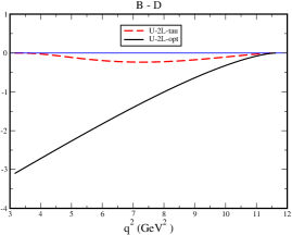
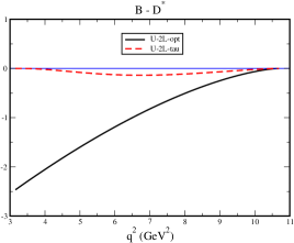
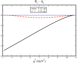
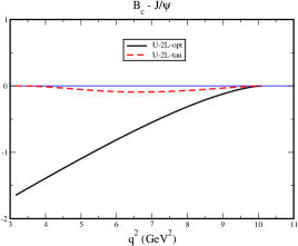
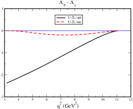
Figure 2: $q^{2}$ dependence of the optimized partial rate $d\Gamma^{\rm optd}_{U-2L}/dq^{2}$ (solid curve) and $d\Gamma_{U-2L}/dq^{2}=v^{3}\,d\Gamma^{\rm optd}_{U-2L}/dq^{2}$ ($\tau$-mode, dashed curve) in units of $10^{-15}$ GeV^-1.

One can then define an experimental branching fraction by writing

$$B(\bar{B}^{0}\to D^{+}\ell^{-}\bar{\nu}_{\ell})=\frac{N(\bar{B}^{0}\to D^{+}\ell^{-}\bar{\nu}_{\ell})}{N(\bar{B}^{0}{\rm-tags})}$$ (37)

which can be compared to the theoretical branching fraction

$$B(\bar{B}^{0}\to D^{+}\ell^{-}\bar{\nu}_{\ell})=\tau(\bar{B}^{0})\Gamma_{\rm tot}(\bar{B}^{0}\to D^{+}\ell^{-}\bar{\nu}_{\ell}).$$ (38)

In the same way one can define an experimental optimized branching fraction by writing

$$B^{\rm optd}_{U-2L}(\bar{B}^{0}\to D^{+}\ell^{-}\bar{\nu}_{\ell})=\frac{N^{\rm optd}_{U-2L}(\bar{B}^{0}\to D^{+}\ell^{-}\bar{\nu}_{\ell})}{N(\bar{B}^{0}-{\rm tags})}$$ (39)

which, again, can be compared to the corresponding theoretical branching fraction

$$B^{\rm optd}_{U-2L}(\bar{B}^{0}\to D^{+}\ell^{-}\bar{\nu}_{\ell})=\tau(\bar{B}^{0})\Gamma^{\rm optd}_{U-2L}(\bar{B}^{0}\to D^{+}\ell^{-}\bar{\nu}_{\ell}).$$ (40)

One then defines optimized rate ratios $R^{\rm optd}_{U-L}(\ell,\ell^{\prime})$ by

$$R^{\rm optd}_{U-L}(\ell,\ell^{\prime})=\frac{B^{\rm optd}_{U-2L}(\ell)}{B^{\rm optd}_{U-2L}(\ell^{\prime})}=\frac{N^{\rm optd}_{U-2L}(\ell)}{N^{\rm optd}_{U-2L}(\ell^{\prime})}=\frac{\Gamma^{\rm optd}_{U-2L}(\ell)}{\Gamma^{\rm optd}_{U-2L}(\ell^{\prime})}\,=\,1,$$ (41)

which are predicted to be equal to one.

As the ratios (41) show, tagging is not really required when measuring the optimized rate ratio $R^{\rm optd}_{U-L}(\ell,\ell^{\prime})$, since the denominators $N(\bar{B}^{0}-{\rm tags})$ drop out when taking the ratio (41). This shows that the optimized rate ratio $R^{\rm optd}_{U-L}(\ell,\ell^{\prime})$ can be experimentally determined even for untagged decays as in the $B_{c}^{-}$ and $\Lambda_{b}$ decays.

VI New Physics Contributions

At present, $b-c$ transition puzzles motivate many studies of New Physics due to the observed deviations from the Standard Model predictions. There is a number of theoretical attempts to resolve these puzzles. See, for example, Refs. Ciezarek:2017yzh ; Becirevic:2016hea and other references therein. Possible NP contributions to the semileptonic decays $\bar{B}^{0}\to D(D^{\ast})\tau^{-}\bar{\nu}_{\tau}$ and $\bar{B}_{c}\to\eta_{c}(J/\psi)\tau^{-}\bar{\nu}_{\tau}$ have been studied in our papers Ivanov:2016qtw ; Tran:2017udy ; Tran:2018kuv . The NP transition form factors have been calculated in the full kinematic $q^{2}$ range employing again the CCQM. The modifications of the partial differential rates $d\Gamma_{U-2L}(\tau)/dq^{2}$ from the differential $(q^{2},\cos\theta)$ distributions of the decays $\bar{B}^{0}\to D\tau^{-}\bar{\nu}_{\tau}$ and $\bar{B}^{0}\to D^{\ast}\tau^{-}\bar{\nu}_{\tau}$ are presented in Eqs. (14) and (C1), respectively, in Ref. Ivanov:2016qtw . One has

$$\frac{d\Gamma_{U-2L}({\rm NP})}{dq^{2}}=\frac{2\Gamma_{0}}{2S_{1}+1}\frac{|\vec{q}\,|q^{2}}{m_{1}^{7}}\,(1-2\delta_{\tau})^{3}\,{\cal H}_{U-2L}({\rm NP})\,,$$ (42)

where

$${\cal H}_{U-2L}({\rm NP})=\left\{\begin{array}[]{ll}-2|1+V_{L}+V_{R}|^{2}|H_{0}|^{2}+32|T_{L}|^{2}|H_{T}|^{2}&\qquad(P-P^{\prime})\text{-transition}\,,\\[6.45831pt] (|1+V_{L}|^{2}+|V_{R}|^{2})(|H_{++}|^{2}+|H_{--}|^{2}-2|H_{00}|^{2})&\\ -4{\rm Re}V_{R}\,(H_{++}H_{--}-|H_{00}|^{2})&\\ -16|T_{L}|^{2}(|H_{T}^{+}|^{2}+|H_{T}^{-}|^{2}-2|H_{T}^{0}|^{2})&\qquad(P-V)\text{-transition}\,.\end{array}\right.$$

If we recall the relations of helicities with the Lorentz form factors then one gets

$${\cal H}_{U-2L+NP}^{P-P^{\prime}} = \frac{4m_{1}^{2}|\vec{q}\,|^{2}}{q^{2}}$$

$$\times \Big{\{}-2\,|1+V_{L}+V_{R}|^{2}\,F^{2}_{+}+32\,|T_{L}|^{2}\,\frac{q^{2}}{m_{+}^{2}}F^{2}_{T}\Big{\}}$$

$$|H_{++}|^{2}+|H_{--}|^{2}-2|H_{00}|^{2} = \frac{2m_{1}^{2}|\vec{q}\,|^{2}}{m_{2}^{2}\,m_{+}^{2}\,q^{2}}$$

$$\times \Big{\{}-(Pq)^{2}\,A_{0}^{2}+2\Big{[}2m_{2}^{2}q^{2}V^{2}+Pq(Pq-q^{2})A_{0}A_{+}\Big{]}-4m_{1}^{2}|\vec{q}\,|^{2}A_{+}^{2}\Big{\}}\,,$$

$$H_{++}H_{--}-|H_{00}|^{2} = \frac{m_{1}^{2}|\vec{q}\,|^{2}}{m_{2}^{2}\,m_{+}^{2}\,q^{2}}$$

$$\times \Big{\{}-(Pq)^{2}\,A_{0}^{2}-2\Big{[}2m_{2}^{2}q^{2}V^{2}-Pq(Pq-q^{2})A_{0}A_{+}\Big{]}-4m_{1}^{2}|\vec{q}\,|^{2}A_{+}^{2}\Big{\}}\,,$$

$$|H_{T}^{+}|^{2}+|H_{T}^{-}|^{2}-2|H_{T}^{0}|^{2} = \frac{2m_{1}^{2}|\vec{q}\,|^{2}}{m_{2}^{2}}\Big{\{}\frac{8m_{2}^{2}}{q^{2}}\,G_{1}^{2}-(G_{1}+G_{2})^{2}$$ (43)

$$+ \frac{2}{m_{+}^{2}}\Big{[}(m_{1}^{2}+3m_{2}^{2}-q^{2})\,G_{1}+(Pq-q^{2})\,G_{2}\Big{]}G_{0}-\frac{4m_{1}^{2}|\vec{q}\,|^{2}}{m_{+}^{4}}\,G_{0}^{2}\Big{\}}\,.$$

One can see that the differential rate $d\Gamma_{U-2L}$ vanishes as $|\vec{q}\,|^{3}$ at zero recoil. Here, $V_{L/R}$ and $T_{L}$ are the complex Wilson coefficients governing the NP contributions. One has to note that the scalar operators contribute to the full four-fold angular distribution but they do not appear in the coefficient proportional to $\cos^{2}\theta$, i.e., in the convexity parameter. It is assumed that NP only affects leptons of the third generation, i.e., the $\tau$ lepton mode. Note that the lepton-mass-dependent factor $v$ also factors out in the NP contributions to the $(U-2L)$ helicity structure function.

The parameters of the dipole approximation for the calculated NP form factors are listed in Eqs. (10) and (11) of Ref. Ivanov:2016qtw for $B-D$ and $B-D^{\ast}$ transitions, and in Table I of the Ref. Tran:2018kuv for $B_{c}-\eta_{c}$ and $B_{c}-J/\psi$ transitions. The allowed regions for the NP Wilson coefficients have been found by fitting the experimental data for the ratios $R(D^{(\ast)})$ by switching on only one of the NP operators at a time.

In each allowed region at $2\sigma$ the best-fit value for each NP coupling was found. The best-fit couplings read

$$\begin{aligned} V_{L}&=-0.23-0.85i,\qquad&V_{R}&=0.03+0.60i,\qquad&T_{L}&=0.38+0.06i.\end{aligned}$$ (44)

We define optimized rates for the NP contributions in the same way as has been done for the SM in Eq. (18). In Fig. 3 we plot the SM differential $q^{2}$ distributions of the optimized rates $d\Gamma_{U-2L}^{\rm optd}/dq^{2}$ together with the corresponding (SM+NP) distributions for the $\tau$-mode. In general, there are four curves for each mode. To avoid oversaturation of the figures, we display the upper and lower curves only and the region between these two curves, colored in yellow. The $P\to P^{\prime}$ optimized differential rates are enhanced by the NP $V_{L}$ and $V_{R}$ contributions, and reduced by the NP tensor contribution $T_{L}$. For the $P\to V$ transitions the enhancement due to the NP tensor contribution $T_{L}$ is quite pronounced over the whole $q^{2}$ range.

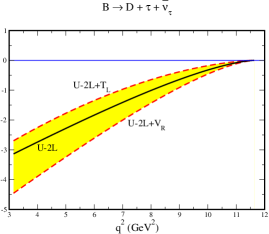
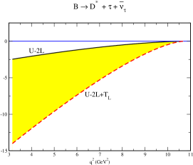
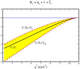
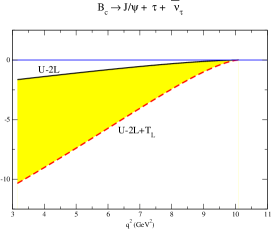
Figure 3: $P\to P^{\prime}\,(V)$ semileptonic transitions taking into account NP effects for the $\tau$ mode. The $q^{2}$ dependence of the optimized partial rates are shown in units of $10^{-15}$ GeV^-1. In the figures we make use of the short hand notation $U-2L=d\Gamma^{\rm optd}_{U-2L}/dq^{2}$.

The enormous size of the NP tensor contribution to the $P\to V$ transitions also shows up in Table 3 where we list the integrated optimized rates and the $\tau/\mu$ ratio of optimized branching fractions

$$R^{\rm optd}_{U-2L}(\tau,\mu)=\frac{\Gamma^{\rm optd}_{U-2L}({\rm SM+NP})}{\Gamma^{\rm optd}_{U-2L}({\rm SM})}\,.$$ (45)

The deviations of the ratio of optimized branching fractions from the SM value of 1 is substantial and huge for the $P\to V$ transitions. One should be remindful of the fact that the NP optimized $\tau$ rates and thereby the ratio of branching fractions $B^{\rm optd}_{U-2L}(\tau,\mu)$ are form-factor dependent.

Table 3: Optimized $(U-2L)$ rates in units of $10^{-14}$ GeV and rate ratios. NP effects are included in the $\tau$-mode only.

Obs.	NP-coupling	$B\to D\ell\nu_{\ell}$	$B_{c}\to\eta_{c}\ell\nu_{\ell}$	$B\to D^{\ast}\ell\nu_{\ell}$	$B_{c}\to J/\psi\ell\nu_{\ell}$
$\Gamma^{\rm optd}_{U-2L}({\rm SM})$		$-1.14$	$-1.21$	$-0.73$	$-0.89$
$\Gamma^{\rm optd}_{U-2L}({\rm SM+NP})$	$V_{L}$	$-1.50$	$-1.59$	$-0.96$	$-0.64$
	$V_{R}$	$-1.62$	$-1.72$	$-0.94$	$-0.62$
	$T_{L}$	$-0.85$	$-0.93$	$-4.46$	$-3.32$
$R^{\rm optd}_{U-2L}(\tau,\mu)$	$V_{L}$	$1.32$	$1.31$	$1.32$	$0.72$
	$V_{R}$	$1.42$	$1.42$	$1.29$	$0.70$
	$T_{L}$	$0.75$	$0.77$	$6.11$	$3.73$

VII Some concluding remarks

As the authors of Ref. Penalva:2019rgt have emphasized, it is important to also have a look at the $(q^{2},E_{\ell})$ distribution in semileptonic decays when testing lepton universality. We briefly discuss the merits of using the $(q^{2},E_{\ell})$ distribution for form-factor-independent tests of lepton universality. One merit of $(q^{2},E_{\ell})$ distribution is obviously that $\cos\theta$ is a derived quantity whereas the lepton energy can be directly measured.

The $(q^{2},\cos\theta)$ distribution (3) can be transformed to the $(q^{2},E_{\ell})$ distribution by making use of the the relation (8) between $\cos\theta$ and $E_{\ell}$. One obtains

$$\frac{d\Gamma}{dq^{2}dE_{\ell}}=\frac{1}{2S_{1}+1}\,\,\frac{3q^{2}}{|\vec{q}\,|^{2}}\frac{\Gamma_{0}}{m_{1}^{7}}\bigg{(}B_{0}(q^{2},m_{\ell})+B_{1}(q^{2},m_{\ell})\Big{(}\frac{E_{\ell}}{m_{1}}\Big{)}+B_{2}(q^{2})\Big{(}\frac{E_{\ell}^{2}}{m_{1}^{2}}\Big{)}\bigg{)}.$$ (46)

where the coefficients $B_{0}(q^{2},m_{\ell}),\,B_{1}(q^{2},m_{\ell})$, and $B_{2}(q^{2})$ are given by

$$B_{0}(q^{2},m_{\ell}) = \frac{1}{4}\Big{(}q_{0}^{2}(1+2\delta_{\ell})^{2}({\cal H}_{U}-2{\cal H}_{L})+v\,|\vec{q}\,|^{2}({\cal H}_{U}+2{\cal H}_{L}+2\delta_{\ell}({\cal H}_{U}+2{\cal H}_{S}))$$ (47)

$$+2q_{0}|\vec{q}\,|(1+2\delta_{\ell})({\cal H}_{P}+4\delta_{\ell}{\cal H}_{SL})\Big{)},$$

$$B_{1}(q^{2},m_{\ell}) = -m_{1}\Big{(}q_{0}(1+2\delta_{\ell})\left({\cal H}_{U}-2{\cal H}_{L}\right)+|\vec{q}\,|\left({\cal H}_{P}+4\delta_{\ell}{\cal H}_{SL}\right)\Big{)},$$ (48)

$$B_{2}(q^{2}) = \,m_{1}^{2}\,\Big{(}{\cal H}_{U}-2{\cal H}_{L}\Big{)}\,.$$ (49)

The $(q^{2},\cos\theta)$ distribution (46) can be seen to be well defined in the limit $|\vec{q}\,|\to 0$ since ${\cal H}_{P},{\cal H}_{SL}\sim|\vec{q}\,|$ and ${\cal H}_{U}-2{\cal H}_{L}\sim|\vec{q}\,|^{2}$ in all three classes of decays as discussed in Sec. IV.

In Fig. 4 we show the $(q^{2},E_{\ell})$ phase space boundaries of the three ($e,\mu,\tau$) modes of the semileptonic decay $\bar{B}^{0}\to D^{+}+\ell^{-}\,\bar{\nu}_{\ell}$. The phase space boundaries are determined by the curves Korner:1989qb ; Kadeer:2005aq

$$q^{2}_{\pm}=\frac{1}{a}\left(b\pm\sqrt{b^{2}-ac}\right),$$ (50)

where

$$a = m_{1}^{2}+m_{\ell}^{2}-2m_{1}E_{\ell},$$

$$b = m_{1}E_{\ell}(m_{1}^{2}-m_{2}^{2}+m_{\ell}^{2}-2m_{1}E_{\ell})+m_{\ell}^{2}m_{2}^{2},$$

$$c = m_{\ell}^{2}\Big{(}(m_{1}^{2}-m_{2}^{2})^{2}+m_{\ell}^{2}m_{1}^{2}-(m_{1}^{2}-m_{2}^{2})2m_{1}E_{\ell}\Big{)}.$$

Figure 4: $(q^{2},E_{\ell})$ phase space for $\bar{B}^{0}\to D^{+}+\ell^{-}+\bar{\nu}_{\ell}$ for the three $(e,\mu,\tau)$ modes.

From the relation (8) linking $\cos\theta$ and $E_{\ell}$ it is not difficult to see that the coefficients of the $\cos^{2}\theta$ and $E^{2}_{\ell}$ terms are simply related. In particular, as Eq. (49) shows, the coefficient $B_{2}(q^{2})$ of the quadratic $E^{2}_{\ell}$ term is proportional to ${\cal H}_{U-2L}$ and, differing from the corresponding coefficient ${\cal H}_{2}$ of the $(q^{2},\cos\theta)$ distribution, does not depend on the lepton mass. A gratifying feature of the $(q^{2},E_{\ell})$ analysis is the fact that the (model dependent) ratio $A_{2}(q^{2})/A_{0}(q^{2},m_{\ell})$ is quite large over the whole $q^{2}$ range Penalva:2019rgt .

Similar to Eq. (15), the second order coefficient $B_{2}(q^{2})=m_{1}^{2}{\cal H}_{U-2L}(q^{2})$ can be projected from the distribution (46) by folding the distribution with the second order Legendre polynomial expressed in terms of the lepton energy, i.e.,

$$P_{2}(\cos\theta(E_{\ell}))=\frac{3}{2}\frac{1}{|\vec{q}\,|^{2}v^{2}}\Big{(}4E_{\ell}^{2}-4E_{\ell}q_{0}(1+2\delta_{\ell})+q_{0}^{2}(1+2\delta_{\ell})^{2}-\frac{1}{3}|\vec{q}\,|^{2}v^{2}\Big{)}.$$ (51)

The folding has to be done within the limits $(E_{\ell}^{+},E_{\ell}^{-})$ where (see, e.g., Refs. Korner:1989qb ; Kadeer:2005aq )

$$E_{\ell}^{\pm}=\frac{1}{2}\Big{(}q_{0}(1+2\delta_{\ell})\pm|\vec{q}\,|\,v\Big{)}.$$ (52)

The zero and first order coefficients $B_{0}$ and $B_{1}$ in Eq. (46) are removed by the folding process since

$$\int_{E_{\ell}-}^{E_{\ell}^{+}}dE_{\ell}P_{2}(\cos\theta(E_{\ell}))=\int_{E_{\ell}-}^{E_{\ell}^{+}}E_{\ell}dE_{\ell}P_{2}(\cos\theta(E_{\ell}))=0$$ (53)

as can be seen by direct calculation or by considering the orthogonality relations

$$\int_{E_{\ell}-}^{E_{\ell}^{+}}dE_{\ell}P_{0,1}(\cos\theta(E_{\ell}))P_{2}(\cos\theta(E_{\ell}))=0.$$ (54)

Similar to Eq. (15) one finds

$$\frac{d\Gamma_{U-2L}}{dq^{2}}=10\int\limits_{E_{\ell}^{-}}^{E_{\ell}^{+}}\!dE_{\ell}\frac{d^{2}\Gamma}{dq^{2}dE_{\ell}}P_{2}(\cos\theta(E_{\ell}))=\frac{2}{2S_{1}+1}\frac{\Gamma_{0}|\vec{q}\,|q^{2}v^{3}}{m_{1}^{7}}{\cal H}_{U-2L}(q^{2}).$$ (55)

To be sure, we have done the somewhat lengthy $E_{\ell}$ integration in Eq. (55) and confirmed the expected result on the r.h.s. of Eq. (55). From here on one would proceed as in Sec. III, i.e., one defines an optimized rate by dividing out the lepton-mass-dependent factor $v^{3}=(1-m^{2}_{\ell}/q^{2})^{3}$. Differing from the $(q^{2},\cos\theta)$ analysis discussed in the main text the $(q^{2},E_{\ell})$ phase space is not rectangular, which means that the $q^{2}$ and $E_{\ell}$ integrations are not interchangeable. The projection of the relevant $B_{2}$ coefficient Eq.(55) has to be done for each $q^{2}$ value, or for each $q^{2}$ bin, before $q^{2}$ integration. In the $\tau$-mode the range of $E_{\ell}$ becomes very small near threshold $q^{2}=m_{\tau}^{2}$ and near the zero-recoil point $q^{2}=(m_{1}-m_{2})^{2}$.

In summary, we have proposed a form-factor-independent test of lepton universality for semileptonic $B$ meson, $B_{c}$ meson, and $\Lambda_{b}$ baryon decays by analyzing the two-fold $(q^{2},\cos\theta)$ decay distribution. We have defined optimized rates for the $e,\mu,\tau$ modes the ratios of which take the value of 1 in the SM, independently of form-factor effects. The form-factor independent test involves a reduced phase space for the light lepton modes which will somewhat reduce the data sample for the light modes. The requisite angular analysis of the two-fold $(q^{2},\cos\theta)$ distribution will be quite challenging from the experimental point of view. We have discussed New Physics effects for the $\tau$-mode the inclusion of which will lead to large aberrations from the SM value of 1 for the ratio of the optimized rates. As a by-line we have also included a discussion of the $(q^{2},E_{\ell})$ decay distribution as a possible candidate for form factor independent tests of lepton universality.

We conclude with two remarks. We have made a wide survey of polarization observables in semileptonic $b$ hadron decays to find an observable with the requisite property that the helicity-flip dependence factors out of the observable. In fact, in semileptonic polarized $\Lambda_{b}$ decay one can identify the observable $v\,({\cal H}_{P}-2{\cal H}_{L_{-}})$ which posesses the desired property Kadeer:2005aq ; Groote:2019rmj . All in all, we are looking forward to experimental tests of lepton universality using the optimized branching ratios proposed in this paper.

- (1) J. Lees et al. (BABAR Collaboration), Phys. Rev. Lett. 109, 101802 (2012) [arXiv:1205.5442 [hep-ex]].
- (2) J. P. Lees et al. (BaBar Collaboration), Phys. Rev. D 88, 072012 (2013) [arXiv:1303.0571 [hep-ex]].
- (3) A. Bozek et al. [Belle], Phys. Rev. D 82, 072005 (2010) [arXiv:1005.2302 [hep-ex]].
- (4) M. Huschle et al. [Belle], Phys. Rev. D 92, no.7, 072014 (2015) [arXiv:1507.03233 [hep-ex]].
- (5) Y. Sato et al. [Belle], Phys. Rev. D 94, no.7, 072007 (2016) [arXiv:1607.07923 [hep-ex]].
- (6) S. Hirose et al. [Belle], Phys. Rev. Lett. 118, no.21, 211801 (2017) [arXiv:1612.00529 [hep-ex]].
- (7) R. Aaij et al. [LHCb], Phys. Rev. Lett. 115, no.11, 111803 (2015) [erratum: Phys. Rev. Lett. 115, no.15, 159901 (2015)] [arXiv:1506.08614 [hep-ex]].
- (8) Y. S. Amhis et al. (HFAG Collaboration), arXiv:1909.12524 [hep-ex].
- (9) F. U. Bernlochner, M. F. Sevilla, D. J. Robinson, and G. Wormser, arXiv:2101.08326 [hep-ex].
- (10) R. Barbieri, [arXiv:2103.15635 [hep-ph]].
- (11) K. Cheung, Z. R. Huang, H. D. Li, C. D. Lü, Y. N. Mao and R. Y. Tang, Nucl. Phys. B 965, 115354 (2021) [arXiv:2002.07272 [hep-ph]].
- (12) T. D. Cohen, H. Lamm, and R. F. Lebed, Phys. Rev. D 100, 094503 (2019) [arXiv:1909.10691 [hep-ph]].
- (13) J. G. Körner and G. A. Schuler, Phys. Lett. B 231, 306 (1989).
- (14) J. G. Körner and G. A. Schuler, Z. Phys. C 46, 93 (1990).
- (15) P. Bialas, J. G. Körner, M. Krämer, and K. Zalewski, Z. Phys. C 57, 115 (1993).
- (16) A. Kadeer, J. G. Körner, and U. Moosbrugger, Eur. Phys. J. C 59, 27 (2009) [hep-ph/0511019].
- (17) T. Gutsche, M. A. Ivanov, J. G. Körner, V. E. Lyubovitskij, P. Santorelli, and N. Habyl, Phys. Rev. D 91, 074001 (2015); D 91, 119907(E) (2015) [arXiv:1502.04864 [hep-ph]].
- (18) M. A. Ivanov, J. G. Körner, and C. T. Tran, Phys. Rev. D 92, 114022 (2015) [arXiv:1508.02678 [hep-ph]].
- (19) S. Groote, J. G. Körner, and B. Melić, Eur. Phys. J. C 79, 948 (2019) [arXiv:1910.00283 [hep-ph]].
- (20) E. Di Salvo, F. Fontanelli, and Z. J. Ajaltouni, Int. J. Mod. Phys. A 33, 1850169 (2018) [arXiv:1804.05592 [hep-ph]].
- (21) M. Fischer, S. Groote, J. G. Körner, and M. C. Mauser, Phys. Rev. D 65, 054036 (2002) [hep-ph/0101322].
- (22) N. Penalva, E. Hernández, and J. Nieves, Phys. Rev. D 100, 113007 (2019) [arXiv:1908.02328 [hep-ph]].
- (23) N. Penalva, E. Hernández, and J. Nieves, Phys. Rev. D 101 (2020) 113004 [arXiv:2004.08253 [hep-ph]].
- (24) N. Penalva, E. Hernández, and J. Nieves, Phys. Rev. D 102, 096016 (2020) [arXiv:2007.12590 [hep-ph]].
- (25) C. S. Kim, S. C. Park and D. Sahoo, Phys. Rev. D 100, no.1, 015005 (2019) [arXiv:1811.08190 [hep-ph]].
- (26) M. Freytsis, Z. Ligeti, and J. T. Ruderman, Phys. Rev. D 92, 054018 (2015) [arXiv:1506.08896 [hep-ph]].
- (27) F. U. Bernlochner and Z. Ligeti, Phys. Rev. D 95, 014022 (2017) [arXiv:1606.09300 [hep-ph]].
- (28) G. Isidori and O. Sumensari, Eur. Phys. J. C 80, 1078 (2020) [arXiv:2007.08481 [hep-ph]].
- (29) W. Detmold, C. Lehner and S. Meinel, Phys. Rev. D 92, no.3, 034503 (2015) [arXiv:1503.01421 [hep-lat]].
- (30) A. Datta, S. Kamali, S. Meinel and A. Rashed, JHEP 08, 131 (2017) [arXiv:1702.02243 [hep-ph]].
- (31) S. Meinel and G. Rendon, [arXiv:2103.08775 [hep-lat]].
- (32) J. A. Bailey et al. [Fermilab Lattice and MILC], Phys. Rev. D 89, no.11, 114504 (2014) [arXiv:1403.0635 [hep-lat]].
- (33) J. A. Bailey et al. [MILC], Phys. Rev. D 92, no.3, 034506 (2015) [arXiv:1503.07237 [hep-lat]].
- (34) H. Na et al. [HPQCD], Phys. Rev. D 92, no.5, 054510 (2015) [erratum: Phys. Rev. D 93, no.11, 119906 (2016)] [arXiv:1505.03925 [hep-lat]].
- (35) D. Bigi and P. Gambino, Phys. Rev. D 94, no.9, 094008 (2016) [arXiv:1606.08030 [hep-ph]].
- (36) F. U. Bernlochner, Z. Ligeti, M. Papucci and D. J. Robinson, Phys. Rev. D 95, no.11, 115008 (2017) [erratum: Phys. Rev. D 97, no.5, 059902 (2018)] [arXiv:1703.05330 [hep-ph]].
- (37) P. Gambino, M. Jung and S. Schacht, Phys. Lett. B 795, 386-390 (2019) [arXiv:1905.08209 [hep-ph]].
- (38) M. Bordone, M. Jung and D. van Dyk, Eur. Phys. J. C 80, no.2, 74 (2020) [arXiv:1908.09398 [hep-ph]].
- (39) C. T. Tran, M. A. Ivanov, J. G. Körner, and P. Santorelli, Phys. Rev. D 97, 054014 (2018) [arXiv:1801.06927 [hep-ph]].
- (40) P. A. Zyla et al. (Particle Data Group), Prog. Theor. Exp. Phys. 2020 (2020) 083C01.
- (41) G. Ciezarek, M. Franco Sevilla, B. Hamilton, R. Kowalewski, T. Kuhr, V. Lüth and Y. Sato, Nature 546, 227-233 (2017) [arXiv:1703.01766 [hep-ex]].
- (42) D. Becirevic, S. Fajfer, I. Nisandzic and A. Tayduganov, Nucl. Phys. B 946, 114707 (2019) [arXiv:1602.03030 [hep-ph]].
- (43) M. A. Ivanov, J. G. Körner, and C. T. Tran, Phys. Rev. D 94, 094028 (2016) [arXiv:1607.02932 [hep-ph]].
- (44) C. T. Tran, M. A. Ivanov and J. G. Körner, [arXiv:1702.06910 [hep-ph]].