Composite Optimization with Coupling Constraints via Dual Proximal Gradient Method with Applications to Asynchronous Networks

Abstract

[Summary]In this paper, we consider solving a composite optimization problem with affine coupling constraints in a multi-agent network based on proximal gradient method. In this problem, all the agents jointly minimize the sum of individual cost functions composed of smooth and possibly non-smooth parts. To this end, we derive the dual problem by the concept of Fenchel conjugate, which gives rise to the dual proximal gradient algorithm by allowing for the asymmetric individual interpretations of the global constraints. Then, an asynchronous dual proximal gradient algorithm is proposed for the asynchronous networks with heterogenous step-sizes and communication delays. For both the two algorithms, if the non-smooth parts of the objective functions are simple-structured, we only need to update dual variables by some simple operations, accounting for the reduction of the overall computational complexity. Analytical convergence rate of the proposed algorithms is derived and their efficacy is verified by solving a social welfare optimization problem of electricity market in the numerical simulation.

1 Introduction

1.1 Background and Motivation

Decentralized optimization has drawn much attention due to its prominent advantage in solving various mathematical optimization problems with large data set and decentralized decision variables in multi-agent networks.^{1, 2, 3} In those problems, each agent usually maintains a local decision variable, and the optimal solution of the system is achieved through multiple rounds of communications and strategy-makings.⁴ In this work, we consider a class of optimization problems with composite cost functions, i.e., composed of smooth (differentiable) and possibly non-smooth (non-differentiable) parts, arising from various fields, such as Lasso regressions, resource allocation problems and support vector machines. ^{5, 6, 7}

To solve those problems, most existing works require the update of primal variables with some costly computations, which increase the overall computational complexity. Meanwhile, with the presence of the asynchrony of large-scale networks in various fields, more explorations on asynchronous optimization algorithms are needed.⁸ As widely discussed, proximal gradient based algorithms can take the advantage of some simple-structured cost functions and are usually numerically more stable than the subgradient based counterparts.⁹ With the above motivation, in this work, we aim to develop an efficient optimization algorithm for decentralized optimization problems (DOPs) based on proximal gradient method and further investigate its efficacy in asynchronous networks.

1.2 Literature Review

In this work, we focus on optimizing a class of composite DOPs subject to affine coupling constraints. To solve these problems, applicable techniques include primal-dual subgradient methods,¹⁰ alternating direction method of multipliers,¹¹ and proximal gradient methods,¹² etc. DOPs with coupling constraints are actively investigated in the recent works,^{13, 14, 15, 16, 17, 18, 19, 20, 21, 22} where the optimal solution to the primal problems is usually achieved with the update of both primal and dual variables. An alternative solution, as discussed by Notarnicola et al.,^{23, 24} is resorting to the dual problems, where the computation on the primal variables is not required. However, the algorithms in References 23 and 24 involve some inner-loop optimization processes, which increase the overall computational complexity if the primal cost functions possess some non-smooth characteristics. To further improve the computational efficiency, dual proximal gradient (DPG) methods for solving composite optimization problems were investigated recently,^{25, 6, 26} where, however, no general affine coupling constraint was considered.

To explore some efficient decentralized algorithms, different from the existing works, the new features of this work are twofold. First, to the best knowledge of the authors, this is the first work that investigates DPG method with general affine constraints with specific network typologies. By the proposed DPG algorithm, the updating of the primal variables is not compulsory. Furthermore, if the proximal mapping of the non-smooth parts in the primal problem can be explicitly given, we only need to update the dual variables by some simple operations, e.g., basic proximal mappings and gradient based iterations, which technically can be more efficient than the existing algorithms with some costly computations on the primal variables or other auxiliary variables.^{13, 14, 15, 16, 17, 18, 19, 20, 21, 22} As another feature, the asymmetric individual interpretation of the agents on the global constraints is considered, where no uniform knowledge of the global constraints is required.

Second, we propose an asynchronous dual proximal gradient (Asyn-DPG) algorithm, which can be viewed as an extension of DPG algorithm by considering heterogenous step-sizes and communication delays. Specifically, the outdated information is addressed through deterministic analysis,^{28, 29, 30, 31, 32, 33, 34, 35} which is advantageous over some stochastic models ³⁶ in the sense that the probability distribution of random factors can be difficult to acquire in some problems and may introduce inaccuracy issues due to limited historical data.³⁷ However, the problem setup in References 28, 29, 31-35 either only considers certain special form of affine coupling constraints or does not incorporate any coupling constraint. In addition, the algorithms discussed in References 30 and 33 dealing with smooth cost functions will hamper their usage in non-smooth optimization problems. Different from all the aforementioned works, we will show that if the upper bound of communication delays is finite and the non-smooth parts in the primal problem are simple-structured, we only need to update dual variables with some simple operations, which is still a distinct advantage to reduce the computational complexity.

We hereby summarize the contributions of this work as follows.

• We consider a class of composite DOPs with both local convex and affine coupling constraints. To solve these problems, a DPG algorithm is proposed by formulating the dual problems. Then, an Asyn-DPG algorithm is built upon the structure of DPG algorithm, which can be applied to asynchronous networks with heterogenous step-sizes and communication delays. In addition, the asymmetric individual interpretations of the global constraints are considered, which is more adaptive to large-scale networks in the sense that no uniform knowledge of the global constraints for the agents is required.

• Provided that the non-smooth parts of the cost functions in the primal DOPs are with some simple structures, the proposed DPG and Asyn-DPG algorithms only require the update of dual variables with some simple operations, accounting for the reduction of the overall computational complexity. In addition, our algorithms require some commonly used assumptions on the primal problems and explicit convergence rates are provided for all the discussed scenarios.

1.3 Paper Structure and Notations

The remainder of this paper is organized as follows. Section 2 presents some frequently used definitions in this work and their properties. Section 3 formulates the primal problem of interest and gives some basic assumptions. In Section 4, two proximal gradient algorithms, namely DPG and Asyn-DPG, are proposed based on different network settings. The convergence analysis of the discussed algorithms is conducted in Section 5. The efficacy of the proposed algorithms is verified by a numerical simulation in Section 6. Section 7 concludes this paper.

$\mathds{N}$ and $\mathds{N}_{+}$ denote the non-negative and positive integer spaces, respectively. Let notation $\mid\mathcal{S}\mid$ be the size of set $\mathcal{S}$. Operator $(\cdot)^{\top}$ represents the transpose of a matrix. $\mathcal{S}_{1}\times\mathcal{S}_{2}$ denotes the Cartesian product of sets $\mathcal{S}_{1}$ and $\mathcal{S}_{2}$. $\mathbf{relint}\mathcal{S}$ represents the relative interior of set $\mathcal{S}$. Let $\lfloor u\rfloor$ ($\lceil u\rceil$) be the largest integer smaller than (smallest integer no smaller than) scalar $u$. $\|\cdot\|_{1}$ and $\|\cdot\|$ refer to the $l_{1}$ and $l_{2}$-norms, respectively. $\langle\cdot,\cdot\rangle$ is an inner product operator. $\otimes$ is the Kronecker product operator. $\mathbf{0}_{n}$ and $\mathbf{1}_{n}$ denote the $n$-dimensional column vectors with all elements being 0 and 1, respectively. $\mathbf{I}_{n}$ and $\mathbf{O}_{n\times m}$ denote the $n$-dimensional identity matrix and $(n\times m)$-dimensional zero matrix, respectively.

2 Preliminaries

In this section, we present some fundamental definitions and properties of graph theory, proximal mapping, and Fenchel conjugate.

2.1 Graph Theory

A multi-agent network can be described by an undirected graph ${\mathcal{G}}=\{{\mathcal{V}},{\mathcal{E}}\}$, which is composed of the set of vertices ${\mathcal{V}}=\{1,2,...,N\}$ and set of edges ${\mathcal{E}}\subseteq\{(i,j)|i,j\in\mathcal{V}\hbox{ and }i\neq j\}$ with $(i,j)\in\mathcal{E}$ an unordered pair (no self-loop). A graph $\mathcal{G}$ is said connected if there exists at least one path between any two distinct vertices. A graph $\mathcal{G}$ is said fully connected if there is a unique edge between any two distinct vertices. ${\mathcal{V}}_{i}=\{j|(i,j)\in\mathcal{E}\}$ denotes the set of the neighbours of agent $i$. Let ${\mathbf{L}}\in\mathds{R}^{N\times N}$ denote the Laplacian matrix of ${\mathcal{G}}$. Let $d_{ij}$ be the element at the cross of the $i$th row and $j$th column of ${\mathbf{L}}$. Thus, $d_{ij}=-1$ if $(i,j)\in{\mathcal{E}}$, $d_{ii}=\mid{\mathcal{V}}_{i}\mid$, and $d_{ij}=0$ otherwise, $i,j\in{\mathcal{V}}$.³⁸

2.2 Proximal Mapping

A proximal mapping of a proper, closed, and convex function $\zeta:\mathds{R}^{n}\rightarrow(-\infty,+\infty]$ is defined by $\mathrm{prox}^{\alpha}_{\zeta}[\mathbf{u}]=\arg\min_{\mathbf{v}}(\zeta(\mathbf{v})+\frac{1}{2{\alpha}}\|\mathbf{v}-\mathbf{u}\|^{2})$ with ${\alpha}>0$ and $\mathbf{u}\in\mathds{R}^{n}$.²⁵

2.3 Fenchel Conjugate

Let $\zeta:\mathds{R}^{n}\rightarrow(-\infty,+\infty]$ be a proper function. The Fenchel conjugate of $\zeta$ is defined as $\zeta^{\diamond}(\mathbf{u})=\sup_{\mathbf{v}}\{\mathbf{u}^{\top}\mathbf{v}-\zeta(\mathbf{v})\}$, which is convex.³⁹ Sec. 3.3

Lemma 1.

(Extended Moreau Decomposition⁴⁰ Thm. 6.45) Let $\zeta:\mathds{R}^{n}\rightarrow(-\infty,+\infty]$ be a proper, closed, convex function and $\zeta^{\diamond}$ be its Fenchel conjugate. Then, for all $\mathbf{u}\in\mathds{R}^{n}$ and $\alpha>0$, we have

$$\mathbf{u}=\alpha\mathrm{prox}^{\frac{1}{\alpha}}_{\zeta^{\diamond}}[\frac{\mathbf{u}}{\alpha}]+\mathrm{prox}^{\alpha}_{\zeta}[\mathbf{u}].$$ (1)

Lemma 2.

Let $\zeta:\mathds{R}^{n}\rightarrow(-\infty,+\infty]$ be a proper, closed, $\sigma$-strongly convex function and $\zeta^{\diamond}$ be its Fenchel conjugate, $\sigma>0$. Then,

$$\nabla_{\mathbf{u}}\zeta^{\diamond}(\mathbf{u})=\arg\max\limits_{\mathbf{v}}(\mathbf{u}^{\top}\mathbf{v}-\zeta(\mathbf{v})),$$ (2)

and $\nabla\zeta^{\diamond}$ is Lipschitz continuous with constant $\frac{1}{\sigma}$.²⁵ Lemma V.7

3 Problem Formulation

The considered optimization problem and relevant assumptions are presented in this section.

Consider a multi-agent network $\mathcal{G}=\{\mathcal{V},\mathcal{E}\}$ and a global cost function $H(\mathbf{x})=\sum_{i\in\mathcal{V}}H_{i}(\mathbf{x}_{i})$, $\mathbf{x}_{i}\in\mathds{R}^{M}$, $\mathbf{x}=[\mathbf{x}^{\top}_{1},...,\mathbf{x}^{\top}_{N}]^{\top}\in\mathds{R}^{{N}M}$. Agent $i$ maintains a private cost function $H_{i}(\mathbf{x}_{i})=f_{i}(\mathbf{x}_{i})+g_{i}(\mathbf{x}_{i})$. Let $\Omega_{i}\subseteq\mathds{R}^{M}$ be the feasible region of $\mathbf{x}_{i}$. Then, the feasible region of $\mathbf{x}$ can be defined by $\Omega=\Omega_{1}\times\Omega_{2}\times...\times\Omega_{N}\subseteq\mathds{R}^{NM}$. We consider a global affine constraint $\mathbf{A}\mathbf{x}=\mathbf{b}$, $\mathbf{A}\in\mathds{R}^{B\times{N}M}$, $\mathbf{b}\in\mathds{R}^{B}$. Then, a DOP of $\mathcal{V}$ can be formulated as

$$\textbf{(P1)}\quad\min\limits_{\mathbf{x}\in\Omega}\quad \sum_{i\in\mathcal{V}}H_{i}(\mathbf{x}_{i})$$

subject to $$\mathbf{A}\mathbf{x}=\mathbf{b}.$$

Assumption 1.

$\mathcal{G}$ is undirected and connected.

Assumption 2.

$f_{i}:\mathds{R}^{M}\rightarrow(-\infty,+\infty]$ is a proper, closed, differentiable, and $\sigma_{i}$-strongly convex extended real-valued function, $\sigma_{i}>0$; $g_{i}:\mathds{R}^{M}\rightarrow(-\infty,+\infty]$ is a proper, closed and convex extended real-valued function, $i\in\mathcal{V}$.

The assumptions in Assumption 2 are often discussed in composite optimization problems.^{41, 42, 43, 44, 45, 6, 25}

Assumption 3.

(Constraint Qualification) $\Omega_{i}$ is non-empty, convex and closed, $i\in\mathcal{V}$; there exists an $\breve{\mathbf{x}}\in\mathbf{relint}\Omega$ such that $\mathbf{A}\breve{\mathbf{x}}=\mathbf{b}$.⁴⁶

In the following, we consider that each agent $i$ maintains a private constraint $\mathcal{X}_{i}=\{\mathbf{x}\in\mathds{R}^{{N}M}|\mathbf{A}^{(i)}\mathbf{x}=\mathbf{b}^{(i)}\}$, which can be regarded as an individual interpretation of the global constraint $\mathcal{X}=\{\mathbf{x}\in\mathds{R}^{{N}M}|\mathbf{A}\mathbf{x}=\mathbf{b}\}$, $\mathbf{A}^{(i)}\in\mathds{R}^{B\times{N}M}$, $\mathbf{b}^{(i)}\in\mathds{R}^{B}$. Therefore, it is reasonable to assume that $\bigcap_{i\in\mathcal{V}}\mathcal{X}_{i}=\mathcal{X}$. Then, Problem (P1) can be equivalently written as

$$\textbf{(P2)}\quad\min\limits_{\mathbf{x}}\quad \sum_{i\in\mathcal{V}}(H_{i}(\mathbf{x}_{i})+\mathds{I}_{\Omega_{i}}(\mathbf{x}_{i}))$$

subject to $$\mathbf{A}^{(i)}\mathbf{x}=\mathbf{b}^{(i)},\quad\forall i\in\mathcal{V},$$

with $\mathds{I}_{\Omega_{i}}(\mathbf{x}_{i})=\left\{\begin{array}[]{ll}0,&\hbox{if $\mathbf{x}_{i}\in\Omega_{i}$},\\ +\infty,&\hbox{otherwise}\end{array}\right.$.⁴⁶

To facilitate the following discussion, we let $\mathbf{A}^{(l)}_{i}\in\mathds{R}^{B\times M}$ denote the $i$th column sub-block of $\mathbf{A}^{(l)}$, i.e., $\mathbf{A}^{(l)}=[\mathbf{A}^{(l)}_{1},...,\mathbf{A}^{(l)}_{i},...,\mathbf{A}^{(l)}_{N}]$, $i,l\in\mathcal{V}$.

Assumption 4.

Assume that $\mathbf{A}^{(i)}\mathbf{x}=\mathbf{b}^{(i)}$ only contains the decision variables of agent $i$ and its neighbours, i.e.,

$$\mathbf{A}^{(i)}_{j}=\mathbf{O}_{B\times M},\quad\forall(i,j)\notin\mathcal{E}\hbox{ and }i\neq j.$$ (3)

Some DOPs complying with Assumption 4 will be discussed in Section 4.2.

4 Dual Proximal Gradient Based Algorithm Development

In this section, we will develop two dual proximal gradient based algorithms for solving the problem of interest under different assumptions on networks.

4.1 Dual Problem

By introducing a slack vector $\mathbf{z}=[\mathbf{z}^{\top}_{1},...,\mathbf{z}^{\top}_{N}]^{\top}$, Problem (P2) can be equivalently written as

$$\textbf{(P3)}\quad\min\limits_{\mathbf{x},\mathbf{z}}\quad \sum_{i\in\mathcal{V}}(f_{i}(\mathbf{x}_{i})+(g_{i}+\mathds{I}_{\Omega_{i}})(\mathbf{z}_{i}))$$

subject to $$\mathbf{A}^{(i)}\mathbf{x}=\mathbf{b}^{(i)},\quad\mathbf{x}_{i}=\mathbf{z}_{i},\quad\forall i\in\mathcal{V}.$$

Then, the Lagrangian function of Problem (P3) can be written as

$$L(\mathbf{x},\mathbf{z},\bm{\theta},\bm{\mu})= \sum_{i\in\mathcal{V}}(f_{i}(\mathbf{x}_{i})+(g_{i}+{\mathds{I}}_{{\Omega}_{i}})(\mathbf{z}_{i})+\bm{\mu}_{i}^{\top}(\mathbf{x}_{i}-\mathbf{z}_{i}))+\sum_{i\in\mathcal{V}}\bm{\theta}_{i}^{\top}(\mathbf{A}^{(i)}\mathbf{x}-\mathbf{b}^{(i)})$$

$$= \sum_{i\in\mathcal{V}}(f_{i}(\mathbf{x}_{i})+(g_{i}+{\mathds{I}}_{{\Omega}_{i}})(\mathbf{z}_{i})+\bm{\mu}_{i}^{\top}(\mathbf{x}_{i}-\mathbf{z}_{i}))+\sum_{i\in\mathcal{V}}\mathbf{x}^{\top}_{i}\sum_{l\in\mathcal{V}}(\mathbf{A}_{i}^{(l)})^{\top}\bm{\theta}_{l}-\sum_{i\in\mathcal{V}}(\mathbf{b}^{(i)})^{\top}\bm{\theta}_{i}$$

$$= \sum_{i\in\mathcal{V}}(f_{i}(\mathbf{x}_{i})+\mathbf{x}_{i}^{\top}(\sum_{l\in\mathcal{V}}(\mathbf{A}^{(l)}_{i})^{\top}\bm{\theta}_{l}+\bm{\mu}_{i})+(g_{i}+{\mathds{I}}_{{\Omega}_{i}})(\mathbf{z}_{i})-\mathbf{z}_{i}^{\top}\bm{\mu}_{i}-(\mathbf{b}^{(i)})^{\top}\bm{\theta}_{i}),$$ (4)

where we use

$$\sum_{i\in\mathcal{V}}\bm{\theta}_{i}^{\top}\mathbf{A}^{(i)}\mathbf{x} =\sum_{i\in\mathcal{V}}\sum_{l\in\mathcal{V}}\bm{\theta}_{i}^{\top}\mathbf{A}_{l}^{(i)}\mathbf{x}_{l}=\sum_{i\in\mathcal{V}}\sum_{l\in\mathcal{V}}\bm{\theta}_{l}^{\top}\mathbf{A}_{i}^{(l)}\mathbf{x}_{i}$$

$$=\sum_{i\in\mathcal{V}}\sum_{l\in\mathcal{V}}\mathbf{x}^{\top}_{i}(\mathbf{A}_{i}^{(l)})^{\top}\bm{\theta}_{l}=\sum_{i\in\mathcal{V}}\mathbf{x}^{\top}_{i}\sum_{l\in\mathcal{V}}(\mathbf{A}_{i}^{(l)})^{\top}\bm{\theta}_{l}$$ (5)

with ${\bm{\theta}}=[\bm{\theta}_{1}^{\top},...,\bm{\theta}_{N}^{\top}]^{\top}\in\mathds{R}^{{N}B}$ and ${\bm{\mu}}=[\bm{\mu}_{1}^{\top},...,\bm{\mu}_{N}^{\top}]^{\top}\in\mathds{R}^{{N}M}$. $\bm{\theta}_{i}$ and $\bm{\mu}_{i}$ denote the Lagrangian multiplier vectors associated with constraints $\mathbf{A}^{(i)}\mathbf{x}=\mathbf{b}^{(i)}$ and $\mathbf{x}_{i}=\mathbf{z}_{i}$, respectively.

Therefore, the dual function can be obtained by minimizing ${L}(\mathbf{x},\mathbf{z},{\bm{\theta}},{\bm{\mu}})$ with $(\mathbf{x},\mathbf{z})$, which gives

$${V}({\bm{\theta}},{\bm{\mu}})= \min\limits_{{\mathbf{x}},{\mathbf{z}}}\sum_{i\in\mathcal{V}}(f_{i}(\mathbf{x}_{i})+\mathbf{x}_{i}^{\top}(\sum_{l\in\mathcal{V}}(\mathbf{A}^{(l)}_{i})^{\top}\bm{\theta}_{l}+\bm{\mu}_{i})+(g_{i}+{\mathds{I}}_{{\Omega}_{i}})(\mathbf{z}_{i})-\mathbf{z}_{i}^{\top}\bm{\mu}_{i}-(\mathbf{b}^{(i)})^{\top}\bm{\theta}_{i})$$

$$= \min\limits_{{\mathbf{x}},{\mathbf{z}}}\sum_{i\in\mathcal{V}}(f_{i}(\mathbf{x}_{i})-\mathbf{x}_{i}^{\top}{\mathbf{C}}_{i}{\bm{\lambda}}+(g_{i}+{\mathds{I}}_{{\Omega}_{i}})(\mathbf{z}_{i})-\mathbf{z}_{i}^{\top}{\mathbf{F}}_{i}{\bm{\lambda}}-{\mathbf{E}}_{i}{\bm{\lambda}})$$

$$= \sum_{i\in\mathcal{V}}(-f^{\diamond}_{i}({\mathbf{C}}_{i}{\bm{\lambda}})-{\mathbf{E}}_{i}{\bm{\lambda}}-(g_{i}+{\mathds{I}}_{{\Omega}_{i}})^{\diamond}({\mathbf{F}}_{i}{\bm{\lambda}})),$$ (6)

where

$${\mathbf{C}}_{i} =[-(\mathbf{A}^{(1)}_{i})^{\top},...,-(\mathbf{A}^{({N})}_{i})^{\top},\mathbf{O}_{M\times(i-1)M},-\mathbf{I}_{M},\mathbf{O}_{M\times({N}-i)M}]\in\mathds{R}^{M\times({N}M+{N}B)},$$ (7)

$${\mathbf{F}}_{i} =[\mathbf{O}_{M\times({N}B+(i-1)M)},\mathbf{I}_{M},\mathbf{O}_{M\times({N}-i)M}]\in\mathds{R}^{M\times({N}M+{N}B)},$$ (8)

$${\mathbf{E}}_{i} =[\mathbf{0}^{\top}_{(i-1)B},(\mathbf{b}^{(i)})^{\top},\mathbf{0}^{\top}_{(N-i)B+NM}]\in\mathds{R}^{1\times({N}M+{N}B)},$$ (9)

$${\bm{\lambda}} =[{\bm{\theta}}^{\top},{\bm{\mu}}^{\top}]^{\top}\in\mathds{R}^{{N}M+{N}B}.$$ (10)

Then, the dual problem of Problem (P3) can be formulated as

$$\textbf{(P4)}\quad\min\limits_{{\bm{\lambda}}}\quad{\Psi}({\bm{\lambda}})$$

where

$${\Psi}({\bm{\lambda}}) ={P}({\bm{\lambda}})+{Q}({\bm{\lambda}}),$$ (11)

$${P}({\bm{\lambda}}) =\sum_{i\in\mathcal{V}}{p}_{i}({\bm{\lambda}}),$$ (12)

$${Q}({\bm{\lambda}}) =\sum_{i\in\mathcal{V}}{q}_{i}({\bm{\mu}_{i}}),$$ (13)

$${p}_{i}({\bm{\lambda}}) =f^{\diamond}_{i}({\mathbf{C}}_{i}{\bm{\lambda}})+{\mathbf{E}}_{i}{\bm{\lambda}},$$ (14)

$${q}_{i}({\bm{\mu}_{i}}) =(g_{i}+{\mathds{I}}_{{\Omega}_{i}})^{\diamond}({\mathbf{F}}_{i}{\bm{\lambda}})=(g_{i}+{\mathds{I}}_{{\Omega}_{i}})^{\diamond}({\bm{\mu}_{i}}).$$ (15)

Define $\mathcal{H}$ as the set of the optimal solutions to Problem (P4).

4.2 Discussion on Constraints

Assumption 4 can be satisfied in some DOPs. See Examples 1 to 4.

Example 1.

$\mathcal{G}$ is fully connected.

Example 2.

In some applications, e.g., telecommunication and machine learning problems, $\mathbf{A}^{(i)}\mathbf{x}=\mathbf{b}^{(i)}$ can be defined by an edge-constraint maintained by agent $i$.⁴⁷

Example 3.

If $\mathbf{A}_{i}^{(i)}=|\mathcal{V}_{i}|\mathbf{I}_{M},\mathbf{A}_{l}^{(i)}=-\mathbf{I}_{M}$, $\mathbf{A}_{j}^{(i)}=\mathbf{O}_{M\times M}$, $\mathbf{b}^{(i)}=\mathbf{0}$, $\forall(i,l)\in\mathcal{E}$, $(i,j)\notin\mathcal{E}\hbox{ and }i\neq j$, then the constraints of Problem (P3) can be written as $\bm{\mathsf{L}}\mathbf{x}=\mathbf{0}$ with $\bm{\mathsf{L}}={\mathbf{L}}\otimes\mathbf{I}_{M}\in\mathds{R}^{NM\times NM}$, which means Problem (P3) essentially is a consensus optimization problem.^{48, 49, 50}

Example 4.

Consider a set of consensus constraints of agent $i$: $\mathbf{x}_{i}-\mathbf{x}_{j}=\mathbf{0}$, $\forall j\in\mathcal{V}_{i}$.²⁵ Then, for any agent pair $(i,j)\in\mathcal{E}$, the individual constraints of agents $i$ and $j$ include $\mathbf{x}_{i}-\mathbf{x}_{j}=\mathbf{0}$ and $\mathbf{x}_{j}-\mathbf{x}_{i}=\mathbf{0}$, respectively. Therefore, the asymmetric constraints can be viewed as a generalization of the asymmetric consensus constraints discussed in this example.

Remark 1.

In Examples 1-4, the asymmetric constraints are more adaptive to large-scale networks in the sense that establishing a global $\mathbf{A}\mathbf{x}=\mathbf{b}$ by integrating the overall decentralized or even distributed constraints may be costly, especially when the network sizes and individual constraints vary constantly.^{51, 52} For example, when certain agent $i$ joins the network, he only needs to broadcast $\mathbf{A}^{(i)}$ to neighbours such that ${\bm{\lambda}}$ can be augmented directly as in Problem (P3), without changing the network-wide constraint architecture seriously by rebuilding $\mathbf{A}\mathbf{x}=\mathbf{b}$.

In practice, the asymmetric individual constraints can be generated by interpreting some common global constraints by user-defined linear transformations. For instance, agent $i$ may interpret constraint $\mathbf{A}\mathbf{x}=\mathbf{b}$ by transformation $\mathbf{T}_{i}\mathbf{A}\mathbf{x}=\mathbf{T}_{i}\mathbf{b}$, i.e., $\mathbf{A}^{(i)}=\mathbf{T}_{i}\mathbf{A}$ and $\mathbf{b}^{(i)}=\mathbf{T}_{i}\mathbf{b}$. See Example 5.

Example 5.

Consider a global affine constraint $\mathcal{X}=\left\{\mathbf{x}\in\mathds{R}^{3}\bigg{|}\left[\begin{array}[]{ccc}1&1&0\\ 2&0&1\\ \end{array}\right]\mathbf{x}=\left[\begin{array}[]{c}1\\ 2\\ \end{array}\right]\right\}$ for a 3-agent network. The individual constraints maintained by agents 1, 2, and 3 are assumed to be

$$\mathcal{X}_{1}= \left\{\mathbf{x}\in\mathds{R}^{3}\bigg{|}\left[\begin{array}[]{ccc}-1&-1&0\\ 1&0&\frac{1}{2}\\ \end{array}\right]\mathbf{x}=\left[\begin{array}[]{c}-1\\ 1\\ \end{array}\right]\right\},$$ (20)

$$\mathcal{X}_{2}= \left\{\mathbf{x}\in\mathds{R}^{3}\big{|}\left[\begin{array}[]{ccc}2&2&0\\ \end{array}\right]\mathbf{x}=2\right\},$$ (22)

$$\mathcal{X}_{3}= \left\{\mathbf{x}\in\mathds{R}^{3}\big{|}\left[\begin{array}[]{ccc}-2&0&-1\\ \end{array}\right]\mathbf{x}=-2\right\},$$ (24)

respectively, where $\mathcal{X}=\mathcal{X}_{1}\bigcap\mathcal{X}_{2}\bigcap\mathcal{X}_{3}$. In this example, $\mathbf{T}_{1}=\left[\begin{array}[]{cc}-1&0\\ 0&\frac{1}{2}\end{array}\right]$, $\mathbf{T}_{2}=\left[\begin{array}[]{cc}2&0\end{array}\right]$, and $\mathbf{T}_{3}=\left[\begin{array}[]{cc}0&-1\end{array}\right]$.

4.3 Dual Proximal Gradient Algorithm

In this subsection, we propose a DPG algorithm to solve Problem (P4). The DPG algorithm is designed as

$${\bm{\lambda}}(k+1)= \mathrm{prox}^{c}_{{Q}}[{\bm{\lambda}}(k)-c\nabla_{{\bm{\lambda}}}{P}({\bm{\lambda}}(k))],$$ (25)

which means

$$\left[\begin{array}[]{c}{\bm{\theta}_{1}}(k+1)\\ \vdots\\ {\bm{\theta}_{N}}(k+1)\\ \bm{\mu}_{1}(k+1)\\ \vdots\\ \bm{\mu}_{N}(k+1)\\ \end{array}\right]= \left[\begin{array}[]{c}{\bm{\theta}_{1}}(k)-c\nabla_{{\bm{\theta}_{1}}}{P}({\bm{\lambda}}(k))\\ \vdots\\ {\bm{\theta}_{N}}(k)-c\nabla_{{\bm{\theta}_{N}}}{P}({\bm{\lambda}}(k))\\ \mathrm{prox}^{c}_{{q}_{1}}[{\bm{\mu}_{1}}(k)-c\nabla_{{\bm{\mu}_{1}}}{P}({\bm{\lambda}}(k))]\\ \vdots\\ \mathrm{prox}^{c}_{{q}_{N}}[{\bm{\mu}_{N}}(k)-c\nabla_{{\bm{\mu}_{N}}}{P}({\bm{\lambda}}(k))]\\ \end{array}\right]$$ (38)

with $\nabla_{{\bm{\lambda}}}{P}=[\nabla^{\top}_{{\bm{\theta}_{1}}}{P},...,\nabla^{\top}_{{\bm{\theta}_{N}}}{P},\nabla^{\top}_{{\bm{\mu}_{1}}}{P},...,\nabla^{\top}_{{\bm{\mu}_{N}}}{P}]^{\top}$ and $c>0$, $k\in\mathds{N}$. The proximal mapping for computing ${\bm{\theta}}$ is omitted since ${\bm{\theta}}$ is not contained by ${Q}$.

To realize decentralized computations, we let the updating of ${\bm{\lambda}}_{i}=[\bm{\theta}_{i}^{\top},{\bm{\mu}_{i}}^{\top}]^{\top}\in\mathds{R}^{B+M}$ be maintained by agent $i$, i.e.,

$${\bm{\lambda}}_{i}(k+1)=\mathrm{prox}^{c}_{{q}_{i}}[{\bm{\lambda}}_{i}(k)-c\nabla_{{\bm{\lambda}}_{i}}{P}({\bm{\lambda}}(k))],$$ (39)

which means

$$\bm{\theta}_{i}(k+1) ={\bm{\theta}_{i}}(k)-c\nabla_{{\bm{\theta}_{i}}}{P}({\bm{\lambda}}(k)),$$ (40)

$${\bm{\mu}_{i}}(k+1) =\mathrm{prox}^{c}_{{q}_{i}}[{\bm{\mu}_{i}}(k)-c\nabla_{{\bm{\mu}_{i}}}{P}({\bm{\lambda}}(k))].$$ (41)

Note that ${\mathbf{F}}_{i}{\bm{\lambda}}=\bm{\mu}_{i}$, hence the variables of ${q}_{i}$ are decoupled from each other. However, each ${p}_{i}({\bm{\lambda}})$ contains the information $\sum_{l\in\mathcal{V}}(\mathbf{A}^{(l)}_{i})^{\top}\bm{\theta}_{l}=\sum_{l\in\mathcal{V}_{i}\cup\{i\}}(\mathbf{A}^{(l)}_{i})^{\top}\bm{\theta}_{l}$ (due to (3)), which means ${P}({\bm{\lambda}})$ is coupled among the neighbouring agents. Therefore, to compute the complete gradient vector $\nabla_{{\bm{\lambda}}_{i}}{P}({\bm{\lambda}}(k))$, agent $i$ needs to collect $\nabla_{{\bm{\lambda}}_{i}}{p}_{l}({\bm{\lambda}}(k))$ from neighbour $l\in\mathcal{V}_{i}$. The communication and computation mechanisms of DPG algorithm are shown in Fig. 1 and Algorithm 1, respectively.

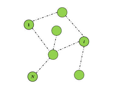
Figure 1: An illustration of the communication mechanism of DPG algorithm. Each agent is only linked to the agents who share the same coupling constraints.

Algorithm 1 Dual Proximal Gradient Algorithm

1:Initialize ${\bm{\lambda}}(0)$ such that ${\Psi}({\bm{\lambda}}(0))\in\mathds{R}$. Determine step-size $c>0$.

2:for $k=0,1,2,...$ do

3:     for $i=1,2,...,{N}$ do (in parallel)

4:         Receive $\nabla_{{\bm{\lambda}}_{i}}{p}_{l}({\bm{\lambda}}(k))$ from neighbour $l\in\mathcal{V}_{i}$.

5:         Update ${\bm{\lambda}}_{i}$ by (39).

6:     end for

7:     Obtain an output ${\bm{\lambda}}^{\mathrm{out}}$ under certain convergence criterion.

8:end for

Remark 2.

As seen in Algorithm 1, compared with symmetric scenarios, the asymmetric individual constraints introduce asymmetric Lagrangian multipliers for the coupling constraints, where the dual variables are decomposed in a natural way and no global consensus of $\bm{\theta}_{i}$ is required.

To apply (39), one need to derive (i) $f^{\diamond}_{i}$ for $\bm{\theta}$ and $\bm{\mu}$ and (ii) the proximal mapping of $(g_{i}+{\mathds{I}}_{{\Omega}_{i}})^{\diamond}$ for $\bm{\mu}$, $i\in\mathcal{V}$. For (i), $f^{\diamond}_{i}$ can be easily obtained if $f_{i}$ is simple-structured, e.g., $f_{i}$ is a quadratic function.⁴⁶ Sec. 3.3.1 For (ii), a feasible method is introduced in the following remark, which can avoid the calculation of the proximal mapping of $(g_{i}+{\mathds{I}}_{{\Omega}_{i}})^{\diamond}$.

Remark 3.

Based on Lemma 1, the updating of $\bm{\mu}_{i}$ in Algorithm 1 can be equivalently written as

$$\bm{\varrho}_{i}(k)={\bm{\mu}_{i}}(k)-c\nabla_{{\bm{\mu}_{i}}}{P}({\bm{\lambda}}(k)),$$ (42)

$$\bm{\mu}_{i}(k+1)=\mathrm{prox}^{c}_{{q}_{i}}[\bm{\varrho}_{i}(k)]=\bm{\varrho}_{i}(k)-c\mathrm{prox}^{\frac{1}{c}}_{{q}^{\diamond}_{i}}[\frac{\bm{\varrho}_{i}(k)}{c}],$$ (43)

with ${q}^{\diamond}_{i}({\bm{\lambda}})=(g_{i}+{\mathds{I}}_{{\Omega}_{i}})^{\diamond\diamond}({\mathbf{F}}_{i}{\bm{\lambda}})=(g_{i}+{\mathds{I}}_{{\Omega}_{i}})({\mathbf{F}}_{i}{\bm{\lambda}})$ due to the convexity and lower semi-continuity of $g_{i}+{\mathds{I}}_{{\Omega}_{i}}$, where $(g_{i}+{\mathds{I}}_{{\Omega}_{i}})^{\diamond\diamond}$ is the biconjugate of $g_{i}+{\mathds{I}}_{{\Omega}_{i}}$.⁴⁶ Sec. 3.3.2 With this arrangement, the calculation of the proximal mapping of $(g_{i}+{\mathds{I}}_{{\Omega}_{i}})^{\diamond}$ is not required as shown in (43), which reduces the computational complexity when the proximal mapping of $g_{i}+{\mathds{I}}_{{\Omega}_{i}}$ is easier to obtain by available formulas.⁴⁰ Sec. 6.3 For example, in some $l_{1}$ regularization problems (e.g., $g_{i}(\mathbf{x}_{i})=\|\mathbf{x}_{i}\|_{1}$, $\Omega_{i}=\mathds{R}^{M}$), the proximal mapping of $l_{1}$-norm is known as the soft thresholding operator with analytical solution.⁴⁰ Sec. 6.3 In addition, if $g_{i}=0$ (i.e., smooth cost functions with local constraints), the proximal mapping of ${\mathds{I}}_{{\Omega}_{i}}$ is an Euclidean projection onto ${\Omega}_{i}$.¹² Sec. 1.2

Additional to the method in Remark 3, the following remark explains how to implement DPG algorithm for certain general form of $g_{i}+{\mathds{I}}_{{\Omega}_{i}}$.

Remark 4.

If the proximal mapping of $g_{i}+{\mathds{I}}_{{\Omega}_{i}}$ cannot be obtained efficiently, a feasible method is to construct a strongly convex $g_{i}$ (e.g., shift a strongly convex component from $f_{i}$ to $g_{i}$). By the definition of proximal mapping, (41) can be rewritten as

$${\bm{\mu}_{i}}(k+1)= \arg\min_{\mathbf{v}}(q_{i}(\mathbf{v})+\frac{1}{2c}\|\mathbf{v}-{\bm{\mu}_{i}}(k)+c\nabla_{{\bm{\mu}_{i}}}{P}({\bm{\lambda}}(k))\|^{2}).$$ (44)

(44) can be solved with gradient descent method by computing the gradient of $q_{i}$ with the help of Lemma 2, i.e.,

$$\nabla_{\mathbf{v}}q_{i}(\mathbf{v})= \nabla_{\mathbf{v}}(g_{i}+{\mathds{I}}_{{X}_{i}})^{\diamond}(\mathbf{v})=\arg\max_{\mathbf{u}}(\mathbf{v}^{\top}\mathbf{u}-(g_{i}+\mathds{I}_{X_{i}})(\mathbf{u})),$$ (45)

which can be completed with local information. In this case, the DPG algorithm can adapt to general nonsmooth $g_{i}+\mathds{I}_{X_{i}}$ with a compromise on an inner-loop optimization process.

4.4 Asynchronous Dual Proximal Gradient Algorithm

In the following, we propose an Asyn-DPG algorithm by extending the usage of DPG algorithm to asynchronous networks.

In synchronous networks, the information accessed by the agents is assumed to be up-to-date, which requires efficient data transmission and can be restrictive for some large-scale networks.⁵³ To address this issue, we propose an Asyn-DPG algorithm for asynchronous networks by considering communication delays. To this end, based on the setup of Problem (P4), we define $\tau(k)$ as the time instant previous to instant $k$ with $k-\tau(k)\geq 0$. Therefore, the accessed dual information at instant $k$ may not be the latest version ${{\bm{\lambda}}}(k)$ but a historical version ${{\bm{\lambda}}}(\tau(k))$. It is reasonable to assume that certain agent always knows the latest information of itself.

Assumption 5.

The communication delays in the network are upper bounded by $D\in\mathds{N}$, which means $0\leq k-\tau(k)\leq D$, $\tau(k)\in\mathds{N}$, $k\in\mathds{N}$.

The upper bound of delays is a commonly used assumption in asynchronous networks.^{55, 28} By allowing for the heterogenous steps-sizes, the proposed Asyn-DPG algorithm is designed as

$${\bm{\lambda}}_{i}(k+1)= \mathrm{prox}^{c_{i}}_{{q}_{i}}[{\bm{\lambda}}_{i}(k)-c_{i}\nabla_{{\bm{\lambda}}_{i}}{P}({\bm{\lambda}}(\tau(k)))].$$ (46)

The computation mechanism of the Asyn-DPG algorithm is shown in Algorithm 2 and Fig. 2.

Algorithm 2 Asynchronous Dual Proximal Gradient Algorithm

1:Initialize ${\bm{\lambda}}(0)$ such that ${\Psi}({\bm{\lambda}}(0))\in\mathds{R}$. Determine step-size $c_{i}>0$, $\forall i\in\mathcal{V}$.

2:for $k=0,1,2,...$ do

3:     for $i=1,2,...,{N}$ do (in parallel)

4:         Receive $\nabla_{{\bm{\lambda}}_{i}}{p}_{l}({\bm{\lambda}}(\tau(k)))$ from neighbour $l\in\mathcal{V}_{i}$.

5:         Update ${\bm{\lambda}}_{i}$ by (46).

6:     end for

7:     Obtain an output ${\bm{\lambda}}^{\mathrm{out}}$ under certain convergence criterion.

8:end for

Note that (46) can be decomposed as indicated in (40) and (41), i.e.,

$$\bm{\theta}_{i}(k+1)= {\bm{\theta}_{i}}(k)-c_{i}\nabla_{{\bm{\theta}_{i}}}{P}({\bm{\lambda}}(\tau(k))),$$ (47)

$${\bm{\mu}_{i}}(k+1)= \mathrm{prox}^{c_{i}}_{{q}_{i}}[{\bm{\mu}_{i}}(k)-c_{i}\nabla_{{\bm{\mu}_{i}}}{P}({\bm{\lambda}}(\tau(k)))].$$ (48)

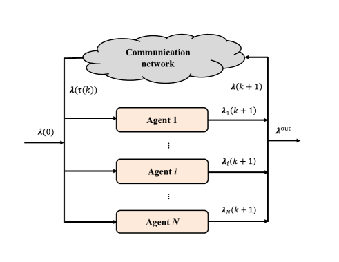
Figure 2: An illustration of the computation mechanism of Asyn-DPG algorithm. Each agent pushes the updated state into the network by using possibly delayed information of others.

Remark 5.

Similar to the discussion in Remark 3, the updating of $\bm{\mu}_{i}$ in Algorithm 2 can be rewritten as

$$\bm{\varrho}^{\prime}_{i}(k)={\bm{\mu}_{i}}(k)-c_{i}\nabla_{{\bm{\mu}_{i}}}{P}({\bm{\lambda}}(\tau(k))),$$ (49)

$$\bm{\mu}_{i}(k+1)=\mathrm{prox}^{c_{i}}_{{q}_{i}}[\bm{\varrho}^{\prime}_{i}(k)]=\bm{\varrho}^{\prime}_{i}(k)-c_{i}\mathrm{prox}^{\frac{1}{c_{i}}}_{{q}^{\diamond}_{i}}[\frac{\bm{\varrho}^{\prime}_{i}(k)}{c_{i}}]$$ (50)

to reduce the computational complexity.

5 Convergence Analysis and Discussion

The convergence analysis of the proposed DPG and Asyn-DPG algorithms is conducted in this section.

Lemma 3.

With Assumption 2, the Lipschitz constant of $\nabla_{{\bm{\lambda}}}{P}({\bm{\lambda}})$ is given by ${h}=\sum_{i\in\mathcal{V}}{h}_{i}$, where ${h}_{i}=\frac{\|{\mathbf{C}}_{i}\|^{2}}{\sigma_{i}}$.

See the proof in Appendix A.

Theorem 1.

Suppose that Assumptions 1-4 hold. Let $\frac{1}{c}={h}$. By Algorithm 1, for any ${\bm{\lambda}}^{*}\in\mathcal{H}$ and $K\in\mathds{N}_{+}$, we have

$${\Psi}({\bm{\lambda}}(K))-{\Psi}({\bm{\lambda}}^{*})\leq\frac{{h}\|{\bm{\lambda}}(0)-{\bm{\lambda}}^{*}\|^{2}}{2K}.$$ (51)

Note that the structure of (25) is consistent with the ISTA algorithm with a constant step-size.⁵⁶ Therefore, the result of Theorem 1 can be deduced with the existing proof by employing the Lipschitz constant ${h}$.⁵⁶ Thm. 3.1 Hence, detailed proof is omitted for simplicity.

Lemma 4.

Based on Assumption 5, for certain $K\in\mathds{N}_{+}$, we have

$$\sum^{K}_{k=0}(\|{\bm{\lambda}}(k+1)-{\bm{\lambda}}(k)\|^{2}+\|{\bm{\lambda}}(k) -{\bm{\lambda}}(k-1)\|^{2}+\cdots+\|{\bm{\lambda}}(\tau(k)+1)-{\bm{\lambda}}(\tau(k))\|^{2})$$

$$\leq\sum^{K}_{k=0}(D+1)\|{\bm{\lambda}}(k+1)-{\bm{\lambda}}(k)\|^{2},$$ (52)

$$\sum^{K}_{k=0}k(\|{\bm{\lambda}}(k+1)-{\bm{\lambda}}(k)\|^{2}+\|{\bm{\lambda}}(k) -{\bm{\lambda}}(k-1)\|^{2}+\cdots+\|{\bm{\lambda}}(\tau(k)+1)-{\bm{\lambda}}(\tau(k))\|^{2})$$

$$\leq\sum_{k=0}^{K}\frac{(2k+D)(D+1)}{2}\|{\bm{\lambda}}(k+1)-{\bm{\lambda}}(k)\|^{2}.$$ (53)

See the proof in Appendix B.

Theorem 2.

Suppose that Assumptions 1-5 hold. By Algorithm 2, given that

$$\frac{1}{c_{i}}\geq{h}(D+1)^{2},$$ (54)

for certain $K\in\mathds{N}_{+}\bigcap[\lceil\frac{D}{2}\rceil,+\infty)$ and any ${\bm{\lambda}}^{*}\in\mathcal{H}$, we have

$${\Psi}({\bm{\lambda}}(K+1))-{\Psi}({\bm{\lambda}}^{*})\leq\frac{\Lambda(c_{1},...,c_{N},D)}{K+1},$$ (55)

where $\Lambda(c_{1},...,c_{N},D)=\sum^{\lfloor\frac{D}{2}\rfloor}_{k=0}\sum_{i\in\mathcal{V}}(\frac{{h}(2k+D)(D+1)^{2}}{4}-\frac{k}{c_{i}})\|{\bm{\lambda}}_{i}(k+1)-{\bm{\lambda}}_{i}(k)\|^{2}+\sum_{i\in\mathcal{V}}\frac{1}{2c_{i}}\|{\bm{\lambda}}_{i}(0)-{\bm{\lambda}}^{*}_{i}\|^{2}$.

See the proof in Appendix C.

6 Numerical Result

In this section, we will verify the feasibility of Algorithms 1 and 2 by considering a social welfare optimization problem in an electricity market with 2 utility companies (UCs) and 3 energy users.

6.1 Simulation Setup

The social welfare optimization problem of the market is formulated as follows.

$$\textbf{(P5)}\quad\min_{\mathbf{x}}\quad \sum_{i\in\mathcal{V}_{\mathrm{UC}}}C_{i}(x^{\mathrm{UC}}_{i})-\sum_{j\in\mathcal{V}_{\mathrm{user}}}U_{j}(x^{\mathrm{user}}_{j})$$

subject to $$\sum_{i\in\mathcal{V}_{\mathrm{UC}}}x^{\mathrm{UC}}_{i}=\sum_{j\in\mathcal{V}_{\mathrm{user}}}x^{\mathrm{user}}_{j},$$ (56)

$$x^{\mathrm{UC}}_{i}\in\Omega^{\textrm{UC}}_{i},\quad\forall i\in\mathcal{V}_{\mathrm{UC}},$$ (57)

$$x^{\mathrm{user}}_{j}\in\Omega^{\textrm{user}}_{j},\quad\forall j\in\mathcal{V}_{\mathrm{user}}.$$ (58)

In Problem (P5), $\mathcal{V}_{\mathrm{UC}}$ and $\mathcal{V}_{\mathrm{user}}$ are the sets of UCs and users, respectively. $\mathbf{x}=[x^{\mathrm{UC}}_{1},...,x^{\mathrm{UC}}_{|\mathcal{V}_{\mathrm{UC}}|},x^{\mathrm{user}}_{1},...,x^{\mathrm{user}}_{|\mathcal{V}_{\mathrm{user}}|}]^{\top}$ with $x^{\mathrm{UC}}_{i}$ and $x^{\mathrm{user}}_{j}$ being the quantities of energy generation and consumption of UC $i$ and user $j$, respectively. $C_{i}(x^{\mathrm{UC}}_{i})$ is the cost function of UC $i$ and $U_{j}(x^{\mathrm{user}}_{j})$ is the utility function of user $j$, $i\in\mathcal{V}_{\mathrm{UC}}$, $j\in\mathcal{V}_{\mathrm{user}}$. The constraint (56) ensures the supply-demand balance in the market. Define constraint matrix ${\mathbf{A}}=[\mathbf{1}^{\top}_{|\mathcal{V}_{\mathrm{UC}}|},-\mathbf{1}^{\top}_{|\mathcal{V}_{\mathrm{user}}|}]$. Then, (56) can be represented by ${\mathbf{A}}\mathbf{x}=0$. $\Omega^{\textrm{UC}}_{i}=[0,x^{\mathrm{UC}}_{i,\mathrm{max}}]$ and $\Omega^{\textrm{user}}_{j}=[0,x^{\mathrm{user}}_{j,\mathrm{max}}]$ are local constraints with $x^{\mathrm{UC}}_{i,\mathrm{max}}>0$ and $x^{\mathrm{user}}_{j,\mathrm{max}}>0$ being the upper bounds of $x^{\mathrm{UC}}_{i}$ and $x^{\mathrm{user}}_{j}$, respectively.

The detailed expressions of $C_{i}(x^{\mathrm{UC}}_{i})$ and $U_{j}(x^{\mathrm{user}}_{j})$ are designed as

$$C_{i}(x^{\mathrm{UC}}_{i})=\kappa_{i}(x^{\mathrm{UC}}_{i})^{2}+\vartheta_{i}x^{\mathrm{UC}}_{i}+\beta_{i},$$ (59)

$$U_{j}(x^{\mathrm{user}}_{j})=\left\{\begin{array}[]{ll}\pi_{j}x^{\mathrm{user}}_{j}-\varsigma_{j}(x^{\mathrm{user}}_{j})^{2},&x^{\mathrm{user}}_{j}\leq\frac{\pi_{j}}{2\varsigma_{j}},\\ \frac{\pi_{j}^{2}}{4\varsigma_{j}},&x^{\mathrm{user}}_{j}>\frac{\pi_{j}}{2\varsigma_{j}},\end{array}\right.$$ (62)

where $\kappa_{i},\vartheta_{i},\beta_{i},\pi_{j},\varsigma_{j}$ are parameters, $\forall i\in\mathcal{V}_{\mathrm{UC}}$, $\forall j\in\mathcal{V}_{\mathrm{user}}$. The values of the parameters are set in Table I.⁵⁷

Table 1: Parameters of UCs and energy users

	UCs			Users
$i/j$	$\kappa_{i}$	$\vartheta_{i}$	$\beta_{i}$	$x^{\mathrm{UC}}_{i,\mathrm{max}}$	$\pi_{j}$	$\varsigma_{j}$	$x^{\mathrm{user}}_{j,\mathrm{max}}$
1	0.0031	8.71	0	150	17.17	0.0935	91.79
2	0.0074	3.53	0	150	12.28	0.0417	147.29
3	-	-	-	-	18.42	0.1007	91.41

To apply the DPG algorithm, we define $\mathbf{A}^{(i),\mathrm{UC}}$ and $\mathbf{A}^{(j),\mathrm{user}}$ as the asymmetric constraint matrices of UC $i$ and user $j$, respectively. Then, by following the derivation of (4.1), the Lagrangian function of Problem (P5) can be obtained as ${L}(\mathbf{x},\mathbf{z},{\bm{\theta}},{\bm{\mu}})$, where ${\bm{\theta}}=[{\theta}^{\mathrm{UC}}_{1},...,{\theta}^{\mathrm{UC}}_{\mid\mathcal{V}_{\mathrm{UC}}\mid},{\theta}^{\mathrm{user}}_{1},...,{\theta}^{\mathrm{user}}_{\mid\mathcal{V}_{\mathrm{user}}\mid}]^{\top}$ and ${\bm{\mu}}=[\mu^{\mathrm{UC}}_{1},...,\mu^{\mathrm{UC}}_{\mid\mathcal{V}_{\mathrm{UC}}\mid},$ ${\mu}^{\mathrm{user}}_{1},...,{\mu}^{\mathrm{user}}_{\mid\mathcal{V}_{\mathrm{user}}\mid}]^{\top}$. See Appendix D for the detailed expressions of ${L}(\mathbf{x},\mathbf{z},{\bm{\theta}},{\bm{\mu}})$, $\mathbf{A}^{(i),\mathrm{UC}}$, and $\mathbf{A}^{(j),\mathrm{user}}$. With some direct calculations, the optimal solution to Problem (P5) is $\mathbf{x}^{*}=[0,150,48.5,50.2,51.3]^{\top}$.

6.2 Simulation Result and Discussion

6.2.1 Simulation 1

To apply Algorithm 1, we consider a fully connected network since all the agents are involved in supply-demand balance constraint. Due to the different individual interpretations of the global constraint, with some linear transformations introduced in Section 4.2, we let $[\mathbf{A}^{(1),\mathrm{UC}},\mathbf{A}^{(2),\mathrm{UC}},\mathbf{A}^{(1),\mathrm{user}},\mathbf{A}^{(2),\mathrm{user}},\mathbf{A}^{(3),\mathrm{user}}]=[\mathbf{T}_{1}\mathbf{A},\mathbf{T}_{2}\mathbf{A},\mathbf{T}_{3}\mathbf{A},\mathbf{T}_{4}\mathbf{A},\mathbf{T}_{5}\mathbf{A}]$, where $\mathbf{T}_{1}=1$, $\mathbf{T}_{2}=2$, $\mathbf{T}_{3}=-1$, $\mathbf{T}_{4}=1$, $\mathbf{T}_{5}=-1$.

The simulation result is shown in Figs. 3 and 4. As shown in Fig. 3, $({\bm{\theta}},{\bm{\mu}})$ converges to certain stationary position $({\bm{\theta}}^{*},{\bm{\mu}}^{*})$. Meanwhile, the optimal solution to the primal problem can be obtained by $\mathbf{x}^{*}=\arg\min_{\mathbf{x}}{L}(\mathbf{x},\mathbf{z},{\bm{\theta}}^{*},{\bm{\mu}}^{*})=[0,150,48.5,50.2,51.3]^{\top}$, and the value of dual function ${\Psi}({\bm{\lambda}})$ (as defined in Problem (P4)) converges to the minimum value ${\Psi}^{*}$, which is around 756.53.

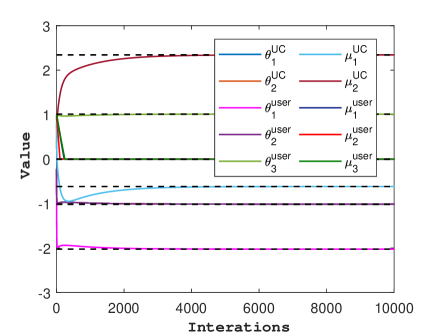
Figure 3: Dynamics of ${\bm{\theta}}$ and ${\bm{\mu}}$.

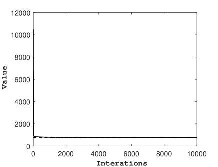
Figure 4: Dynamics of ${\Psi}({\bm{\lambda}})$.

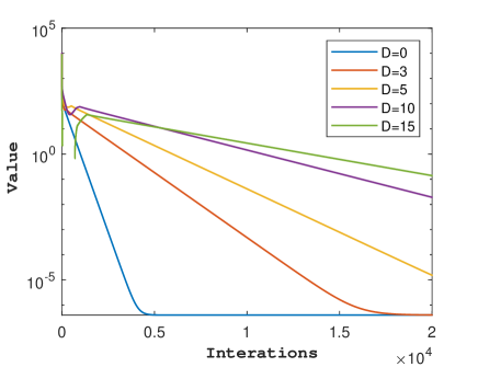
Figure 5: Dynamics of $\epsilon$ with different delays.

6.2.2 Simulation 2

To apply Algorithm 2, the upper bound of communication delays is set as $D\in\{0,3,5,10,15\}$. To represent the “worst delays”, we let $\tau(k)=\max\{0,k-D\}$, $k\in\mathds{N}$. In addition, we define $\epsilon(k)={\Psi}({\bm{\lambda}}(k))-{\Psi}^{*}$ to characterize the dynamics of convergence error.

With the same asymmetric constraints in Simulation 1, the simulation result is shown in Fig. 5. It can be seen that, with different delays, the minimum of ${\Psi}({\bm{\lambda}})$, i.e., ${\Psi}^{*}$, is achieved asymptotically, which implies the optimal solution to the primal problem is achieved since Simulations 1 and 2 are based on the same setup of Problem (P4). In Fig. 5, one can also note that a larger delay can slower the convergence speed, which is consistent with result (55), i.e., a larger value of $D$ can produce a larger error bound in certain step.

7 Conclusion

In this work, we focused on optimizing a class of composite DOPs with both local convex and affine coupling constraints. With different network settings, two dual proximal gradient based algorithms were proposed. As the key feature, all the discussed algorithms resort to the dual problem. Provided that the non-smooth parts of the cost functions are simple-structured, we only need to update dual variables with some simple operations, which leads to the reduction of the overall computational complexity.

Appendix A Proof of Lemma 3

By the $\frac{1}{\sigma_{i}}$-Lipschitz continuity of $\nabla f^{\diamond}_{i}$ (see Lemma 2 and Assumption 2), we have

$$\|\nabla_{\mathbf{u}}f^{\diamond}_{i}(\mathbf{C}_{i}\mathbf{u})-\nabla_{\mathbf{v}}f^{\diamond}_{i}(\mathbf{C}_{i}\mathbf{v})\|= \|\mathbf{C}_{i}^{\top}(\nabla_{\mathbf{C}_{i}\mathbf{u}}f^{\diamond}_{i}(\mathbf{C}_{i}\mathbf{u})-\nabla_{\mathbf{C}_{i}\mathbf{v}}f^{\diamond}_{i}(\mathbf{C}_{i}\mathbf{v}))\|\leq\|\mathbf{C}_{i}\|\|\nabla_{\mathbf{C}_{i}\mathbf{u}}f^{\diamond}_{i}(\mathbf{C}_{i}\mathbf{u})-\nabla_{\mathbf{C}_{i}\mathbf{v}}f^{\diamond}_{i}(\mathbf{C}_{i}\mathbf{v})\|$$

$$\leq \frac{\|\mathbf{C}_{i}\|}{\sigma_{i}}\|\mathbf{C}_{i}\mathbf{u}-\mathbf{C}_{i}\mathbf{v}\|\leq\frac{\|\mathbf{C}_{i}\|^{2}}{\sigma_{i}}\|\mathbf{u}-\mathbf{v}\|=h_{i}\|\mathbf{u}-\mathbf{v}\|,$$ (63)

$\forall\mathbf{u},\mathbf{v}\in\mathds{R}^{NM+NB}$, which means $\nabla_{\bm{\lambda}}f^{\diamond}_{i}(\mathbf{C}_{i}\bm{\lambda})$ is $h_{i}$-Lipschitz continuous and, therefore, $\nabla_{\bm{\lambda}}p_{i}(\bm{\lambda})=\nabla_{\bm{\lambda}}f^{\diamond}(\mathbf{C}_{i}\bm{\lambda})+\mathbf{E}_{i}^{\top}$ is also $h_{i}$-Lipschitz continuous. Then, the Lipschitz constant of $\nabla_{{\bm{\lambda}}}{P}({\bm{\lambda}})$ is a linear sum of ${h}_{i}$, which gives ${h}$, $i\in\mathcal{V}$.

Appendix B Proof of Lemma 4

For (52),

$$\sum^{K}_{k=0}(\|{\bm{\lambda}}(k+1)-{\bm{\lambda}}(k)\|^{2}+\|{\bm{\lambda}}(k)-{\bm{\lambda}}(k-1)\|^{2}+\cdots+\|{\bm{\lambda}}(\tau(k)+1)-{\bm{\lambda}}(\tau(k))\|^{2})$$

$$= (\|{\bm{\lambda}}(K+1)-{\bm{\lambda}}(K)\|^{2}+\|{\bm{\lambda}}(K)-{\bm{\lambda}}(K-1)\|^{2}+\cdots+\|{\bm{\lambda}}(\tau(K)+1)-{\bm{\lambda}}(\tau(K))\|^{2})$$

$$+(\|{\bm{\lambda}}(K)-{\bm{\lambda}}(K-1)\|^{2}+\|{\bm{\lambda}}(K-1)-{\bm{\lambda}}(K-2)\|^{2}+\cdots+\|{\bm{\lambda}}(\tau(K-1)+1)-{\bm{\lambda}}(\tau(K-1))\|^{2})+\cdots$$

$$+(\|{\bm{\lambda}}(2)-{\bm{\lambda}}(1)\|^{2}+\|{\bm{\lambda}}(1)-{\bm{\lambda}}(0)\|^{2})+\|{\bm{\lambda}}(1)-{\bm{\lambda}}(0)\|^{2}$$

$$\leq \|{\bm{\lambda}}(K+1)-{\bm{\lambda}}(K)\|^{2}+2\|{\bm{\lambda}}(K)-{\bm{\lambda}}(K-1)\|^{2}+\cdots+(D+1)\|{\bm{\lambda}}(\tau(K)+1)-{\bm{\lambda}}(\tau(K))\|^{2}+\cdots$$

$$+(D+1)\|{\bm{\lambda}}(1)-{\bm{\lambda}}(0)\|^{2}$$

$$\leq \sum^{K}_{k=0}(D+1)\|{\bm{\lambda}}(k+1)-{\bm{\lambda}}(k)\|^{2}.$$ (64)

For (53),

$$\sum^{K}_{k=0}k(\|{\bm{\lambda}}(k+1)-{\bm{\lambda}}(k)\|^{2}+\|{\bm{\lambda}}(k)-{\bm{\lambda}}(k-1)\|^{2}+\cdots+\|{\bm{\lambda}}(\tau(k)+1)-{\bm{\lambda}}(\tau(k))\|^{2})$$

$$= K(\|{\bm{\lambda}}(K+1)-{\bm{\lambda}}(K)\|^{2}+\|{\bm{\lambda}}(K)-{\bm{\lambda}}(K-1)\|^{2}+\cdots+\|{\bm{\lambda}}(\tau(K)+1)-{\bm{\lambda}}(\tau(K))\|^{2})$$

$$+(K-1)(\|{\bm{\lambda}}(K)-{\bm{\lambda}}(K-1)\|^{2}+\cdots+\|{\bm{\lambda}}(\tau(K-1)+1)-{\bm{\lambda}}(\tau(K-1))\|^{2})+\cdots$$

$$+1\cdot(\|{\bm{\lambda}}(2)-{\bm{\lambda}}(1)\|^{2}+\|{\bm{\lambda}}(1)-{\bm{\lambda}}(0)\|^{2})+0\cdot\|{\bm{\lambda}}(1)-{\bm{\lambda}}(0)\|^{2}$$

$$\leq K\|{\bm{\lambda}}(K+1)-{\bm{\lambda}}(K)\|^{2}+((K-1)+K)\|{\bm{\lambda}}(K)-{\bm{\lambda}}(K-1)\|^{2}+\cdots$$

$$+(k+(k+1)+\cdots+(k+D))\|{\bm{\lambda}}(k+1)-{\bm{\lambda}}(k)\|^{2}+\cdots+(0+1+\cdots+D)\|{\bm{\lambda}}(1)-{\bm{\lambda}}(0)\|^{2}$$

$$\leq \sum_{k=0}^{K}(k+(k+1)+\cdots+(k+D))\|{\bm{\lambda}}(k+1)-{\bm{\lambda}}(k)\|^{2}$$

$$= \sum_{k=0}^{K}\frac{(2k+D)(D+1)}{2}\|{\bm{\lambda}}(k+1)-{\bm{\lambda}}(k)\|^{2}.$$ (65)

Appendix C Proof of Theorem 2

For agent $i$, by the first-order optimality condition of proximal mapping (46), we have

$$\mathbf{0}\in \nabla_{{\bm{\lambda}}_{i}}{P}({\bm{\lambda}}(\tau(k)))+\partial{q}_{i}({\bm{\lambda}}_{i}(k+1))+\frac{1}{c_{i}}({\bm{\lambda}}_{i}(k+1)-{\bm{\lambda}}_{i}(k)).$$ (66)

By the convexity of ${q}_{i}$, we have

$${q}_{i}({\bm{\lambda}}_{i}(k+1))-{q}_{i}({\bm{\lambda}}_{i})\leq \langle\nabla_{{\bm{\lambda}}_{i}}{P}({\bm{\lambda}}(\tau(k))),{\bm{\lambda}}_{i}-{\bm{\lambda}}_{i}(k+1)\rangle+\frac{1}{c_{i}}\langle{\bm{\lambda}}_{i}(k+1)-{\bm{\lambda}}_{i}(k),{\bm{\lambda}}_{i}-{\bm{\lambda}}_{i}(k+1)\rangle.$$ (67)

Summing up (67) over $\mathcal{V}$ gives

$${Q}({\bm{\lambda}}(k+1))-{Q}({\bm{\lambda}})\leq \langle\nabla_{{\bm{\lambda}}}{P}({\bm{\lambda}}(\tau(k))),{\bm{\lambda}}-{\bm{\lambda}}(k+1)\rangle+\sum_{i\in\mathcal{V}}\frac{1}{c_{i}}\langle{\bm{\lambda}}_{i}(k+1)-{\bm{\lambda}}_{i}(k),{\bm{\lambda}}_{i}-{\bm{\lambda}}_{i}(k+1)\rangle,$$ (68)

where the separability of ${Q}$ is used. By the Lipschitz continuity of $\nabla_{{\bm{\lambda}}}{P}$ and convexity of ${P}$, we have

$${P}({\bm{\lambda}}(k+1))-{P}({\bm{\lambda}}(\tau(k)))\leq \langle\nabla_{{\bm{\lambda}}}{P}({\bm{\lambda}}(\tau(k))),{\bm{\lambda}}(k+1)-{\bm{\lambda}}(\tau(k))\rangle+\frac{{h}}{2}\|{\bm{\lambda}}(k+1)-{\bm{\lambda}}(\tau(k))\|^{2}$$

$$\leq {P}({\bm{\lambda}})-\langle\nabla_{{\bm{\lambda}}}{P}({\bm{\lambda}}(\tau(k))),{\bm{\lambda}}-{\bm{\lambda}}(\tau(k))\rangle+\langle\nabla_{{\bm{\lambda}}}{P}({\bm{\lambda}}(\tau(k))),{\bm{\lambda}}(k+1)-{\bm{\lambda}}(\tau(k))\rangle$$

$$+\frac{{h}}{2}\|{\bm{\lambda}}(k+1)-{\bm{\lambda}}(\tau(k))\|^{2}$$

$$\leq {P}({\bm{\lambda}})+\langle\nabla_{{\bm{\lambda}}}{P}({\bm{\lambda}}(\tau(k))),{\bm{\lambda}}(k+1)-{\bm{\lambda}}\rangle+\frac{{h}}{2}\|{\bm{\lambda}}(k+1)-{\bm{\lambda}}(\tau(k))\|^{2}.$$ (69)

Adding together the both sides of (68) and (C) gives

$${\Psi}({\bm{\lambda}}(k+1))-{\Psi}({\bm{\lambda}})\leq \sum_{i\in\mathcal{V}}\frac{1}{c_{i}}\langle{\bm{\lambda}}_{i}(k+1)-{\bm{\lambda}}_{i}(k),{\bm{\lambda}}_{i}-{\bm{\lambda}}_{i}(k+1)\rangle+\frac{{h}}{2}\|{\bm{\lambda}}(k+1)-{\bm{\lambda}}(\tau(k))\|^{2}$$

$$= \frac{{h}}{2}\|{\bm{\lambda}}(k+1)-{\bm{\lambda}}(\tau(k))\|^{2}-\sum_{i\in\mathcal{V}}\frac{1}{2c_{i}}\|{\bm{\lambda}}_{i}(k+1)-{\bm{\lambda}}_{i}(k)\|^{2}$$

$$+\sum_{i\in\mathcal{V}}\frac{1}{2c_{i}}(\|{\bm{\lambda}}_{i}(k)-{\bm{\lambda}}_{i}\|^{2}-\|{\bm{\lambda}}_{i}(k+1)-{\bm{\lambda}}_{i}\|^{2}),$$ (70)

where relation $\mathbf{u}^{\top}\mathbf{v}=\frac{1}{2}(\|\mathbf{u}\|^{2}+\|\mathbf{v}\|^{2}-\|\mathbf{u}-\mathbf{v}\|^{2})$ is used, $\forall\mathbf{u},\mathbf{v}\in\mathds{R}^{M+B}$. By letting ${\bm{\lambda}}={\bm{\lambda}}^{*}$ in (C) and summing up the result over $k=0,...,K$, we have

$$\sum_{n=0}^{K}({\Psi}({\bm{\lambda}}(k+1))-{\Psi}({\bm{\lambda}}^{*}))\leq \sum_{k=0}^{K}(\frac{{h}}{2}\|{\bm{\lambda}}(k+1)-{\bm{\lambda}}(\tau(k))\|^{2}-\sum_{i\in\mathcal{V}}\frac{1}{2c_{i}}\|{\bm{\lambda}}_{i}(k+1)-{\bm{\lambda}}_{i}(k)\|^{2}$$

$$+\sum_{i\in\mathcal{V}}\frac{1}{2c_{i}}(\|{\bm{\lambda}}_{i}(k)-{\bm{\lambda}}^{*}_{i}\|^{2}-\|{\bm{\lambda}}_{i}(k+1)-{\bm{\lambda}}^{*}_{i}\|^{2}))$$

$$\leq \sum_{k=0}^{K}(\frac{{h}(D+1)}{2}(\|{\bm{\lambda}}(k+1)-{\bm{\lambda}}(k)\|^{2}+\cdots+\|{\bm{\lambda}}(\tau(k)+1)-{\bm{\lambda}}(\tau(k))\|^{2})$$

$$-\sum_{i\in\mathcal{V}}\frac{1}{2c_{i}}\|{\bm{\lambda}}_{i}(k+1)-{\bm{\lambda}}_{i}(k)\|^{2}+\sum_{i\in\mathcal{V}}\frac{1}{2c_{i}}(\|{\bm{\lambda}}_{i}(k)-{\bm{\lambda}}^{*}_{i}\|^{2}-\|{\bm{\lambda}}_{i}(k+1)-{\bm{\lambda}}^{*}_{i}\|^{2}))$$

$$\leq \sum_{k=0}^{K}(\frac{{h}(D+1)^{2}}{2}\|{\bm{\lambda}}(k+1)-{\bm{\lambda}}(k)\|^{2}-\sum_{i\in\mathcal{V}}\frac{1}{2c_{i}}\|{\bm{\lambda}}_{i}(k+1)-{\bm{\lambda}}_{i}(k)\|^{2}$$

$$+\sum_{i\in\mathcal{V}}\frac{1}{2c_{i}}(\|{\bm{\lambda}}_{i}(k)-{\bm{\lambda}}^{*}_{i}\|^{2}-\|{\bm{\lambda}}_{i}(k+1)-{\bm{\lambda}}^{*}_{i}\|^{2}))$$

$$\leq \sum_{k=0}^{K}\sum_{i\in\mathcal{V}}(\frac{{h}(D+1)^{2}}{2}-\frac{1}{2c_{i}})\|{\bm{\lambda}}_{i}(k+1)-{\bm{\lambda}}_{i}(k)\|^{2}+\sum_{i\in\mathcal{V}}\frac{1}{2c_{i}}\|{\bm{\lambda}}_{i}(0)-{\bm{\lambda}}^{*}_{i}\|^{2},$$ (71)

where Cauchy-Schwarz inequality and (52) are used in the second and third inequalities, respectively. Letting ${\bm{\lambda}}={\bm{\lambda}}(k)$ in (C) gives

$${\Psi}({\bm{\lambda}}(k+1))-{\Psi}({\bm{\lambda}}(k))\leq \frac{{h}}{2}\|{\bm{\lambda}}(k+1)-{\bm{\lambda}}(\tau(k))\|^{2}-\sum_{i\in\mathcal{V}}\frac{1}{c_{i}}\|{\bm{\lambda}}_{i}(k+1)-{\bm{\lambda}}_{i}(k)\|^{2}.$$ (72)

Multiplying (72) by $k$ and summing up the result over $k=0,1,...,K$ gives

$$\sum_{k=0}^{K}k({\Psi}({\bm{\lambda}}(k+1))-{\Psi}({\bm{\lambda}}(k)))= \sum_{k=0}^{K}((k+1){\Psi}({\bm{\lambda}}(k+1))-k{\Psi}({\bm{\lambda}}(k))-{\Psi}({\bm{\lambda}}(k+1)))$$

$$= (K+1){\Psi}({\bm{\lambda}}(K+1))-\sum_{n=0}^{K}{\Psi}({\bm{\lambda}}(k+1))$$

$$\leq \sum^{K}_{k=0}k(\frac{{h}}{2}\|{\bm{\lambda}}(k+1)-{\bm{\lambda}}(\tau(k))\|^{2}-\sum_{i\in\mathcal{V}}\frac{1}{c_{i}}\|{\bm{\lambda}}_{i}(k+1)-{\bm{\lambda}}_{i}(k)\|^{2})$$

$$\leq \sum^{K}_{k=0}k(\frac{{h}(D+1)}{2}(\|{\bm{\lambda}}(k+1)-{\bm{\lambda}}(k)\|^{2}+\cdots+\|{\bm{\lambda}}(\tau(k)+1)-{\bm{\lambda}}(\tau(k))\|^{2})$$

$$-\sum_{i\in\mathcal{V}}\frac{1}{c_{i}}\|{\bm{\lambda}}_{i}(k+1)-{\bm{\lambda}}_{i}(k)\|^{2})$$

$$\leq \sum^{K}_{k=0}\sum_{i\in\mathcal{V}}(\frac{{h}(2k+D)(D+1)^{2}}{4}-\frac{k}{c_{i}})\|{\bm{\lambda}}_{i}(k+1)-{\bm{\lambda}}_{i}(k)\|^{2},$$ (73)

where (53) is used in the last inequality. By adding the both sides of (C) and (C) together, we have

$$(K+1)({\Psi}({\bm{\lambda}}(K+1))-{\Psi}({\bm{\lambda}}^{*}))\leq \sum_{k=0}^{K}\sum_{i\in\mathcal{V}}(\frac{{h}(D+1)^{2}}{2}-\frac{1}{2c_{i}})\|{\bm{\lambda}}_{i}(k+1)-{\bm{\lambda}}_{i}(k)\|^{2}$$

$$+\sum^{K}_{k=0}\sum_{i\in\mathcal{V}}(\frac{{h}(2k+D)(D+1)^{2}}{4}-\frac{k}{c_{i}})\|{\bm{\lambda}}_{i}(k+1)-{\bm{\lambda}}_{i}(k)\|^{2}+\sum_{i\in\mathcal{V}}\frac{1}{2c_{i}}\|{\bm{\lambda}}_{i}(0)-{\bm{\lambda}}^{*}_{i}\|^{2}$$

$$= \sum_{k=0}^{K}\sum_{i\in\mathcal{V}}(\frac{{h}(D+1)^{2}}{2}-\frac{1}{2c_{i}})\|{\bm{\lambda}}_{i}(k+1)-{\bm{\lambda}}_{i}(k)\|^{2}$$

$$+\sum^{\lfloor\frac{D}{2}\rfloor}_{k=0}\sum_{i\in\mathcal{V}}(\frac{{h}(2k+D)(D+1)^{2}}{4}-\frac{k}{c_{i}})\|{\bm{\lambda}}_{i}(k+1)-{\bm{\lambda}}_{i}(k)\|^{2}$$

$$+\sum^{K}_{k=\lceil\frac{D}{2}\rceil}\sum_{i\in\mathcal{V}}(\frac{{h}(2k+D)(D+1)^{2}}{4}-\frac{k}{c_{i}})\|{\bm{\lambda}}_{i}(k+1)-{\bm{\lambda}}_{i}(k)\|^{2}+\sum_{i\in\mathcal{V}}\frac{1}{2c_{i}}\|{\bm{\lambda}}_{i}(0)-{\bm{\lambda}}^{*}_{i}\|^{2}$$

$$= \sum_{k=0}^{K}\sum_{i\in\mathcal{V}}(\underbrace{\frac{{h}(D+1)^{2}}{2}-\frac{1}{2c_{i}}}_{=\varpi_{1}})\|{\bm{\lambda}}_{i}(k+1)-{\bm{\lambda}}_{i}(k)\|^{2}$$

$$+\sum^{\lfloor\frac{D}{2}\rfloor}_{k=0}\sum_{i\in\mathcal{V}}(\frac{{h}(2k+D)(D+1)^{2}}{4}-\frac{k}{c_{i}})\|{\bm{\lambda}}_{i}(k+1)-{\bm{\lambda}}_{i}(k)\|^{2}+\sum^{K}_{k=\lceil\frac{D}{2}\rceil}\sum_{i\in\mathcal{V}}(k(\underbrace{\frac{{h}(D+1)^{2}}{2}-\frac{1}{2c_{i}}}_{=\varpi_{2}})$$

$$+(\underbrace{\frac{{h}D(D+1)^{2}}{4}-\frac{k}{2c_{i}}}_{=\varpi_{3}}))\|{\bm{\lambda}}_{i}(k+1)-{\bm{\lambda}}_{i}(k)\|^{2}+\sum_{i\in\mathcal{V}}\frac{1}{2c_{i}}\|{\bm{\lambda}}_{i}(0)-{\bm{\lambda}}^{*}_{i}\|^{2}$$

$$\leq \sum^{\lfloor\frac{D}{2}\rfloor}_{k=0}\sum_{i\in\mathcal{V}}(\frac{{h}(2k+D)(D+1)^{2}}{4}-\frac{k}{c_{i}})\|{\bm{\lambda}}_{i}(k+1)-{\bm{\lambda}}_{i}(k)\|^{2}+\sum_{i\in\mathcal{V}}\frac{1}{2c_{i}}\|{\bm{\lambda}}_{i}(0)-{\bm{\lambda}}^{*}_{i}\|^{2}$$

$$= \Lambda(c_{1},...,c_{N},D),$$ (74)

where $\varpi_{1},\varpi_{2},\varpi_{3}\leq 0$ with $\frac{1}{c_{i}}\geq{h}(D+1)^{2}$, $i\in\mathcal{V}$. This proves (55) .

Appendix D Matrices and Lagrangian Function in Section 6

The asymmetric constraint matrices of UC $i$ and user $j$ are given by

$$\mathbf{A}^{(i),\mathrm{UC}}= [A_{1}^{(i),\mathrm{UC}},...,A_{\mid\mathcal{V}_{\mathrm{UC}}\mid}^{(i),\mathrm{UC}},A_{\mid\mathcal{V}_{\mathrm{UC}}\mid+1}^{(i),\mathrm{UC}},...,A_{\mid\mathcal{V}_{\mathrm{UC}}\mid+\mid\mathcal{V}_{\mathrm{user}}\mid}^{(i),\mathrm{UC}}],$$ (75)

$$\mathbf{A}^{(j),\mathrm{user}}= [A_{1}^{(j),\mathrm{user}},...,A_{\mid\mathcal{V}_{\mathrm{UC}}\mid}^{(j),\mathrm{user}},A_{\mid\mathcal{V}_{\mathrm{UC}}\mid+1}^{(j),\mathrm{user}},...,A_{\mid\mathcal{V}_{\mathrm{UC}}\mid+\mid\mathcal{V}_{\mathrm{user}}\mid}^{(j),\mathrm{user}}].$$ (76)

Similar to the derivation of (4.1), based on (75) and (76), one can have

$${L}(\mathbf{x},\mathbf{z},{\bm{\theta}},{\bm{\mu}})= \sum_{i\in\mathcal{V}_{\mathrm{UC}}}(C_{i}(x^{\mathrm{UC}}_{i})+\mathds{I}_{\Omega^{\textrm{UC}}_{i}}(z^{\mathrm{UC}}_{i}))+\sum_{j\in\mathcal{V}_{\mathrm{user}}}(-U_{j}(x^{\mathrm{user}}_{j})+\mathds{I}_{\Omega^{\textrm{user}}_{j}}(z^{\mathrm{user}}_{j}))$$

$$+\sum_{i\in\mathcal{V}_{\mathrm{UC}}}x^{\mathrm{UC}}_{i}(\sum_{l\in\mathcal{V}_{\mathrm{UC}}}{A}^{(l),\mathrm{UC}}_{i}{\theta}^{\mathrm{UC}}_{l}+\sum_{l^{\prime}\in\mathcal{V}_{\mathrm{user}}}{A}^{(l^{\prime}),\mathrm{user}}_{i}{\theta}^{\mathrm{user}}_{l^{\prime}}+{\mu}^{\mathrm{UC}}_{i})$$

$$+\sum_{j\in\mathcal{V}_{\mathrm{user}}}x^{\mathrm{user}}_{j}(\sum_{l\in\mathcal{V}_{\mathrm{UC}}}{A}^{(l),\mathrm{UC}}_{\mid\mathcal{V}_{\mathrm{UC}}\mid+j}{\theta}^{\mathrm{UC}}_{l}+\sum_{l^{\prime}\in\mathcal{V}_{\mathrm{user}}}{A}^{(l^{\prime}),\mathrm{user}}_{\mid\mathcal{V}_{\mathrm{UC}}\mid+j}{\theta}^{\mathrm{user}}_{l^{\prime}}+{\mu}^{\mathrm{user}}_{j})$$

$$-\sum_{i\in\mathcal{V}_{\mathrm{UC}}}z^{\mathrm{UC}}_{i}{\mu}^{\mathrm{UC}}_{i}-\sum_{j\in\mathcal{V}_{\mathrm{user}}}z^{\mathrm{user}}_{j}{\mu}^{\mathrm{user}}_{j}.$$ (77)

References

- 1 Luo L, Chakraborty N, Sycara K. Provably-good distributed algorithm for constrained multi-robot task assignment for grouped tasks. IEEE Transactions on Robotics 2014; 31(1): 19–30.
- 2 Lee K, Lam M, Pedarsani R, Papailiopoulos D, Ramchandran K. Speeding up distributed machine learning using codes. IEEE Transactions on Information Theory 2017; 64(3): 1514–1529.
- 3 Bai L, Ye M, Sun C, Hu G. Distributed economic dispatch control via saddle point dynamics and consensus algorithms. IEEE Transactions on Control Systems Technology 2017; 27(2): 898–905.
- 4 Yuan D, Xu S, Zhang B, Rong L. Distributed primal-dual stochastic subgradient algorithms for multi-agent optimization under inequality constraints. International Journal of Robust and Nonlinear Control 2013; 23(16): 1846–1868.
- 5 Hans C. Bayesian lasso regression. Biometrika 2009; 96(4): 835–845.
- 6 Beck A, Teboulle M. A fast dual proximal gradient algorithm for convex minimization and applications. Operations Research Letters 2014; 42(1): 1–6.
- 7 Zhao SY, Xiang R, Shi YH, Gao P, Li WJ. Scope: Scalable composite optimization for learning on spark. Thirty-First AAAI Conference on Artificial Intelligence 2017.
- 8 Bertsekas DP, Tsitsiklis JN. Parallel and distributed computation: numerical methods. 23. Prentice hall Englewood Cliffs, NJ . 1989.
- 9 Bertsekas DP. Incremental proximal methods for large scale convex optimization. Mathematical Programming 2011; 129(2): 163.
- 10 Nesterov Y. Primal-dual subgradient methods for convex problems. Mathematical programming 2009; 120(1): 221–259.
- 11 Wang Y, Yin W, Zeng J. Global convergence of ADMM in nonconvex nonsmooth optimization. Journal of Scientific Computing 2019; 78(1): 29–63.
- 12 Parikh N, Boyd S. Proximal algorithms. Foundations and Trends in Optimization 2014; 1(3): 127–239.
- 13 Mateos-Núnez D, Cortés J. Distributed saddle-point subgradient algorithms with Laplacian averaging. IEEE Transactions on Automatic Control 2016; 62(6): 2720–2735.
- 14 Necoara I, Nedelcu V, Clipici D, Toma L. On fully distributed dual first order methods for convex network optimization. IFAC-PapersOnLine 2017; 50(1): 2788–2793.
- 15 Notarnicola I, Notarstefano G. Constraint-coupled distributed optimization: a relaxation and duality approach. IEEE Transactions on Control of Network Systems 2019; 7(1): 483–492.
- 16 Li X, Feng G, Xie L. Distributed Proximal Algorithms for Multi-Agent Optimization with Coupled Inequality Constraints. IEEE Transactions on Automatic Control 2020.
- 17 Falsone A, Margellos K, Garatti S, Prandini M. Distributed constrained convex optimization and consensus via dual decomposition and proximal minimization. 2016 IEEE 55th Conference on Decision and Control (CDC) 2016: 1889–1894.
- 18 Falsone A, Margellos K, Garatti S, Prandini M. Dual decomposition for multi-agent distributed optimization with coupling constraints. Automatica 2017; 84: 149–158.
- 19 Zhu M, Martínez S. On distributed convex optimization under inequality and equality constraints. IEEE Transactions on Automatic Control 2011; 57(1): 151–164.
- 20 Chang TH. A proximal dual consensus ADMM method for multi-agent constrained optimization. IEEE Transactions on Signal Processing 2016; 64(14): 3719–3734.
- 21 Chang TH, Nedić A, Scaglione A. Distributed constrained optimization by consensus-based primal-dual perturbation method. IEEE Transactions on Automatic Control 2014; 59(6): 1524–1538.
- 22 Simonetto A, Jamali-Rad H. Primal recovery from consensus-based dual decomposition for distributed convex optimization. Journal of Optimization Theory and Applications 2016; 168(1): 172–197.
- 23 Notarnicola I, Notarstefano G. A duality-based approach for distributed optimization with coupling constraints. IFAC-PapersOnLine 2017; 50(1): 14326–14331.
- 24 Notarnicola I, Franceschelli M, Notarstefano G. A duality-based approach for distributed min–max optimization. IEEE Transactions on Automatic Control 2018; 64(6): 2559–2566.
- 25 Notarnicola I, Notarstefano G. Asynchronous distributed optimization via randomized dual proximal gradient. IEEE Transactions on Automatic Control 2016; 62(5): 2095–2106.
- 26 Kim D, Fessler JA. Fast dual proximal gradient algorithms with rate for convex minimization. arXiv preprint arXiv:1609.09441 2016.
- 27 Necoara I, Nedelcu V. On linear convergence of a distributed dual gradient algorithm for linearly constrained separable convex problems. Automatica 2015; 55: 209–216.
- 28 Zhou Y, Liang Y, Yu Y, Dai W, Xing EP. Distributed proximal gradient algorithm for partially asynchronous computer clusters. The Journal of Machine Learning Research 2018; 19(1): 733–764.
- 29 Chang TH, Hong M, Liao WC, Wang X. Asynchronous distributed ADMM for large-scale optimization - Part I: Algorithm and convergence analysis. IEEE Transactions on Signal Processing 2016; 64(12): 3118–3130.
- 30 Hale MT, Nedić A, Egerstedt M. Asynchronous multiagent primal-dual optimization. IEEE Transactions on Automatic Control 2017; 62(9): 4421–4435.
- 31 Nedic A, Bertsekas DP. Incremental subgradient methods for nondifferentiable optimization. SIAM Journal on Optimization 2001; 12(1): 109–138.
- 32 Cannelli L, Facchinei F, Scutari G, Kungurtsev V. Asynchronous Optimization over Graphs: Linear Convergence under Error Bound Conditions. IEEE Transactions on Automatic Control 2020.
- 33 Tian Y, Sun Y, Scutari G. Achieving Linear Convergence in Distributed Asynchronous Multiagent Optimization. IEEE Transactions on Automatic Control 2020; 65(12): 5264–5279.
- 34 Li M, Zhou L, Yang Z, et al. Parameter server for distributed machine learning. Big Learning NIPS Workshop 2013; 6: 2.
- 35 Hong M. A distributed, asynchronous, and incremental algorithm for nonconvex optimization: an ADMM approach. IEEE Transactions on Control of Network Systems 2017; 5(3): 935–945.
- 36 Cannelli L, Facchinei F, Kungurtsev V, Scutari G. Asynchronous parallel algorithms for nonconvex optimization. Mathematical Programming 2019: 1–34.
- 37 Bertsekas DP, Tsitsiklis JN. Introduction to probability. 1. Athena Scientific Belmont, MA . 2002.
- 38 Chung FR, Graham FC. Spectral graph theory. No. 92American Mathematical Soc. . 1997.
- 39 Borwein J, Lewis AS. Convex analysis and nonlinear optimization: theory and examples. Springer Science & Business Media . 2010.
- 40 Beck A. First-order methods in optimization. SIAM . 2017.
- 41 Shi W, Ling Q, Wu G, Yin W. A proximal gradient algorithm for decentralized composite optimization. IEEE Transactions on Signal Processing 2015; 63(22): 6013–6023.
- 42 Wang Q, Chen J, Zeng X, Xin B. Distributed proximal-gradient algorithms for nonsmooth convex optimization of second-order multiagent systems. International Journal of Robust and Nonlinear Control 2020; 30(17): 7574–7592.
- 43 Schmidt M, Roux N, Bach F. Convergence Rates of Inexact Proximal-Gradient Methods for Convex Optimization. Advances in Neural Information Processing Systems 2011; 24: 1458–1466.
- 44 Chang TH, Hong M, Wang X. Multi-agent distributed optimization via inexact consensus ADMM. IEEE Transactions on Signal Processing 2014; 63(2): 482–497.
- 45 Florea MI, Vorobyov SA. A generalized accelerated composite gradient method: Uniting Nesterov’s fast gradient method and FISTA. IEEE Transactions on Signal Processing 2020; 68: 3033–3048.
- 46 Boyd S, Boyd SP, Vandenberghe L. Convex optimization. Cambridge University Press . 2004.
- 47 Zhang G, Heusdens R. Distributed optimization using the primal-dual method of multipliers. IEEE Transactions on Signal and Information Processing over Networks 2017; 4(1): 173–187.
- 48 Sun C, Ye M, Hu G. Distributed time-varying quadratic optimization for multiple agents under undirected graphs. IEEE Transactions on Automatic Control 2017; 62(7): 3687–3694.
- 49 Wen G, Duan Z, Yu W, Chen G. Consensus in multi-agent systems with communication constraints. International Journal of Robust and Nonlinear Control 2012; 22(2): 170–182.
- 50 Yuan D, Xu S, Lu J. Gradient-free method for distributed multi-agent optimization via push-sum algorithms. International Journal of Robust and Nonlinear Control 2015; 25(10): 1569–1580.
- 51 Franceschelli M, Frasca P. Stability of Open Multiagent Systems and Applications to Dynamic Consensus. IEEE Transactions on Automatic Control 2020; 66(5): 2326–2331.
- 52 Chen T, Giannakis GB. Bandit convex optimization for scalable and dynamic IoT management. IEEE Internet of Things Journal 2018; 6(1): 1276–1286.
- 53 Chou CT, Cidon I, Gopal IS, Zaks S. Synchronizing asynchronous bounded delay networks. IEEE Transactions on Communications 1990; 38(2): 144–147.
- 54 Guo Z, Chen G. Distributed zero-gradient-sum algorithm for convex optimization with time-varying communication delays and switching networks. International Journal of Robust and Nonlinear Control 2018; 28(16): 4900–4915.
- 55 Wang X, Saberi A, Stoorvogel AA, Grip HF, Yang T. Consensus in the network with uniform constant communication delay. Automatica 2013; 49(8): 2461–2467.
- 56 Beck A, Teboulle M. A fast iterative shrinkage-thresholding algorithm for linear inverse problems. SIAM Journal on Imaging Sciences 2009; 2(1): 183–202.
- 57 Pourbabak H, Luo J, Chen T, Su W. A novel consensus-based distributed algorithm for economic dispatch based on local estimation of power mismatch. IEEE Transactions on Smart Grid 2017; 9(6): 5930–5942.