A Thin Self-Stabilizing Asynchronous Unison Algorithm with Applications to Fault Tolerant Biological Networks

Abstract

Introduced by Emek and Wattenhofer (PODC 2013), the stone age (SA) model provides an abstraction for network algorithms distributed over randomized finite state machines. This model, designed to resemble the dynamics of biological processes in cellular networks, assumes a weak communication scheme that is built upon the nodes’ ability to sense their vicinity in an asynchronous manner. Recent works demonstrate that the weak computation and communication capabilities of the SA model suffice for efficient solutions to some core tasks in distributed computing, but they do so under the (somewhat less realistic) assumption of fault free computations. In this paper, we initiate the study of self-stabilizing SA algorithms that are guaranteed to recover from any combination of transient faults. Specifically, we develop efficient self-stabilizing SA algorithms for the leader election and maximal independent set tasks in bounded diameter graphs subject to an asynchronous scheduler. These algorithms rely on a novel efficient self-stabilizing asynchronous unison (AU) algorithm that is “thin” in terms of its state space: the number of states used by the AU algorithm is linear in the graph’s diameter bound, irrespective of the number of nodes.

1 Introduction

A fundamental dogma in distributed computing is that a distributed algorithm cannot be deployed in a real system unless it can cope with faults. When it comes to recovering from transient faults, the agreed upon concept for fault tolerance is self-stabilization. Introduced in the seminal paper of Dijkstra [Dij74], an algorithm is self-stabilizing if it is guaranteed to converge to a correct output from any (possibly faulty) initial configuration [Dol00, ADDP19].

Similarly to distributed man-made digital systems, self-stabilization is also crucial to the survival of biological distributed systems. Indeed, these systems typically lack a central component that can determine the initial system configuration in a coordinated manner and more often than not, they are exposed to environmental conditions that may lead to transient faults. On the other hand, biological distributed systems are often inferior to man-made distributed systems in terms of the computation and communication capabilities of their individual components (e.g., a single cell in an organ), thus calling for a different model of distributed network algorithms.

Aiming to capture distributed processes in biological cellular networks, Emek and Wattenhofer [EW13] introduced the stone age (SA) model that provides an abstraction for distributed algorithms in a network of randomized finite state machines that communicate with their network neighbors using a fixed message alphabet based on a weak communication scheme. Since then, the power and limitations of distributed SA algorithms have been studied in several papers. In particular, it has been established that some of the most fundamental tasks in the field of distributed graph algorithms can be solved efficiently in this restricted model [EW13, AEK18a, AEK18b, EU20]. However, for the most part, the existing literature on the SA model focuses on fault free networks and little is known about self-stabilizing distributed algorithms operating under this model.

In the current paper, we strive to change this situation: Focusing on graphs of bounded diameter, we design efficient self-stabilizing SA algorithms for leader election and maximal independent set — two of the most fundamental and extensively studied tasks in the theory of distributed computing. A key technical component in the algorithms we design is a self-stabilizing synchronizer for SA algorithms in graphs of bounded diameter. This synchronizer relies on a novel anonymous size-uniform self-stabilizing algorithm for the asynchronous unison task [CFG92, AKM⁺93] that operates with a number of states linear in the graphs diameter bound $D$. To the best of our knowledge, this is the first self-stabilizing asynchronous unison algorithm for graphs of general topology whose state space is expressed solely as a function of $D$, independently of the number $n$ of nodes.

The decision to focus on bounded diameter graphs is motivated by regarding this graph family as a natural extension of complete graphs. Indeed, environmental obstacles may disconnect (permanently or temporarily) some links in an otherwise fully connected network, thus increasing its diameter beyond one, but hopefully not to the extent of exceeding a certain fixed upper bound. Fully connected networks go hand in hand with broadcast communication that prevail in the context of both man-made (e.g., contention resolution in multiple access channels) and biological (e.g., quorum sensing in bacterial populations) distributed processes. As the SA model offers a (weak form) of broadcast communication, it makes sense to investigate its power and limitations in such networks and their natural extensions.

1.1 Computational Model

The computational model used in this paper is a simplified version of the stone age (SA) model of Emek and Wattenhofer [EW13]. This model captures anonymous size-uniform distributed algorithms with bounded memory nodes that exchange information by means of an asynchronous variant of the set-broadcast communication scheme (cf. [HJK⁺15]) with no sender collision detection (cf. [AAB⁺11]). Formally, given a distributed task $\mathcal{T}$ defined over a set $\mathcal{O}$ of output values, an algorithm $\Pi$ for $\mathcal{T}$ is encoded by the $4$-tuple $\Pi=\left\langle Q,Q_{\mathcal{O}},\omega,\delta\right\rangle$, where

• $Q$ is a set of states;

• $Q_{\mathcal{O}}\subseteq Q$ is a set of output states;

• $\omega:Q_{\mathcal{O}}\to\mathcal{O}$ is a surjective function that maps each output state to an output value; and

• $\delta:Q\times\left\{0,1\right\}^{Q}\to 2^{Q}$ is a state transition function (to be explained soon).

We would eventually require that the state space of $\Pi$, namely, the size $|Q|$ of the state set, is fixed, and in particular independent of the graph on which $\Pi$ runs, as defined in [EW13]. To facilitate the discussion though, let us relax this requirement for the time being.

Consider a finite connected undirected graph $G=(V,E)$. A configuration of $G$ is a function $\mathcal{C}:V\to Q$ that determines the state $\mathcal{C}(v)\in Q$ of node $v$ for each $v\in V$. We say that a node $v\in V$ senses state $q\in Q$ under $\mathcal{C}$ if there exists some (at least one) node $u\in\mathit{N}^{+}(v)$ such that $\mathcal{C}(u)=q$. The signal of $v$ under $\mathcal{C}$ is the binary vector $\mathcal{S}_{v}^{\mathcal{C}}\in\{0,1\}^{Q}$ defined so that $\mathcal{S}_{v}^{\mathcal{C}}(q)=1$ if and only if $v$ senses state $q\in Q$; in other words, the signal of node $v$ allows $v$ to determine for each state $q\in Q$ whether $q$ appears in its (inclusive) neighborhood, but it does not allow $v$ to count the number of such appearances, nor does it allow $v$ to identify the neighbors residing in state $q$.

The execution of $\Pi$ progresses in discrete steps, where step $t\in\mathbb{Z}_{\geq 0}$ spans the time interval $[t,t+1)$. Let $\mathcal{C}^{t}:V\to Q$ be the configuration of $G$ at time $t$ and let $\mathcal{S}_{v}^{t}=\mathcal{S}_{v}^{\mathcal{C}^{t}}$ denote the signal of node $v\in V$ under $\mathcal{C}^{t}$. We consider an asynchronous schedule defined by means of a sequence of node activations (cf. a distributed fair daemon [DT11]). Formally, a malicious adversary, who knows $\Pi$ but is oblivious to the nodes’ coin tosses, determines the initial configuration $\mathcal{C}^{0}$ and a subset $A^{t}\subseteq V$ of nodes to be activated at time $t$ for each $t\in\mathbb{Z}_{\geq 0}$. If node $v\in V$ is not activated at time $t$, then $\mathcal{C}^{t+1}(v)=\mathcal{C}^{t}(v)$. Otherwise ($v\in A^{t}$), the state of $v$ is updated in step $t$ from $\mathcal{C}^{t}(v)$ to $\mathcal{C}^{t+1}(v)$ picked uniformly at random from $\delta\left(\mathcal{C}^{t}(v),\mathcal{S}_{v}^{t}\right)$. We emphasize that all nodes $v\in V$ obey the same state transition function $\delta$.

Fix some schedule $\{A^{t}\}_{t\geq 0}$. The adversary is required to prevent “node starvation” in the sense that each node must be activated infinitely often. Given a time $t\in\mathbb{Z}_{\geq 0}$, let $\varrho(t)$ be the earliest time satisfying the property that for every node $v\in V$, there exists a time $t\leq t^{\prime}<\varrho(t)$ such that $v\in A_{t^{\prime}}$. This allows us to introduce the round operator $\varrho^{i}(t)$ defined by setting $\varrho^{0}(t)=t$ and $\varrho^{i}(t)=\varrho\left(\varrho^{i-1}(t)\right)$ for $i=1,2,\dots$ Denote $R(i)=\varrho^{i}(0)$ for $i=0,1,\dots$, and observe that if $R(i)\leq t<R(i+1)$, then $R(i+1)\leq\varrho(t)<R(i+2)$.

A configuration $\mathcal{C}:V\to Q$ is said to be an output configuration if $\mathcal{C}(v)\in Q_{\mathcal{O}}$ for every $v\in V$, in which case, we regard $\omega(\mathcal{C}(v))$ as the output of node $v$ under $\mathcal{C}$ and refer to $\omega\circ\mathcal{C}$ as the output vector of $\mathcal{C}$. We say that the execution of $\Pi$ on $G$ has stabilized by time $t\in\mathbb{Z}_{\geq 0}$ if (1) $\mathcal{C}^{t^{\prime}}$ is an output configuration for every $t^{\prime}\geq t$; and (2) the output vector sequence $\{\omega\circ\mathcal{C}^{t^{\prime}}\}_{t^{\prime}\geq t}$ satisfies the requirements of the distributed task $\mathcal{T}$ for which $\Pi$ is defined (the requirements of the distributed tasks studied in the current paper are presented in Sec. 1.2).

The algorithm is self-stabilizing if for any choice of initial configuration $\mathcal{C}^{0}$ and schedule $\{A^{t}\}_{t\geq 0}$, the probability that $\Pi$ has stabilized by time $R(i)$ goes to $1$ as $i\to\infty$. We refer to the smallest $i$ for which the execution has stabilized by time $R(i)$ as the stabilization time of this execution. The stabilization time of a randomized (self-stabilizing) algorithm on a given graph is a random variable and one typically aims towards bounding it in expectation and whp.

The schedule $\{A^{t}\}_{t\geq 0}$ is said to be synchronous if $A^{t}=V$ for all $t\in\mathbb{Z}_{\geq 0}$ which means that $R(i)=i$ for $i=0,1,\dots$ A (self-stabilizing) algorithm whose correctness and stabilization time guarantees hold under the assumption of a synchronous schedule is called a synchronous algorithm. We sometime emphasize that an algorithm does not rely on this assumption by referring to it as an asynchronous algorithm.

1.2 Distributed Tasks

In this paper, we focus on three classic (and extensively studied) distributed tasks, defined over a finite connected undirected graph $G=(V,E)$. In the first task, called asynchronous unison (AU) [CFG92] (a.k.a. distributed pulse [AKM⁺93]), each node in $V$ outputs a clock value taken from an (additive) cyclic group $K$. The task is then defined by the following two conditions: The safety condition requires that if two neighboring nodes output clock values $\kappa\in K$ and $\kappa^{\prime}\in K$, then $\kappa^{\prime}\in\{\kappa-1,\kappa,\kappa+1\}$, where the $+1$ and $-1$ operations are with respect to $K$. The liveness condition requires that for every (post stabilization) time $t$ and for every $i\in\mathbb{Z}_{>0}$, each node updates its clock value at least $i$ times during the time interval $[t,\varrho^{\operatorname{diam}(G)+i}(t))$, where $\operatorname{diam}(G)$ denotes the diameter of $G$; these updates are performed by and only by applying the $+1$ operation of $K$.

The other two distributed tasks considered in this paper are leader election (LE) and maximal independent set (MIS). Both tasks are defined over a binary set $\mathcal{O}=\{0,1\}$ of output values and are static in the sense that once the algorithm has stabilized, its output vector remains fixed. In LE, it is required that exactly one node in $V$ outputs $1$; in MIS, it is required that the set $U\subseteq V$ of nodes that output $1$ is independent, i.e., $(U\times U)\cap E=\emptyset$, whereas any proper superset of $U$ is not independent. We note that LE and MIS correspond to global and local mutual exclusion, respectively, and that the two tasks coincide if $G$ is the complete graph.

1.3 Contribution

In what follows, we refer to the class of graphs whose diameter is up-bounded by $D$ as $D$-bounded diameter. Our first result comes in the form of developing a new self-stabilizing AU algorithm.

Theorem 1.1.

The class of $D$-bounded diameter graphs admits a deterministic self-stabilizing AU algorithm that operates with state space $O(D)$ and stabilizes in time $O(D^{3})$.

To the best of our knowledge, the algorithm promised in Thm. 1.1 is the first self-stabilizing AU algorithm for general graphs $G=(V,E)$ with state space linear in the diameter bound $D$, irrespective of any other graph parameter including $n=|V|$. This remains true even when considering algorithms designed to work under much stronger computational models (see Sec. 5 for further discussion). Moreover, to the best of our knowledge, this is also the first anonymous size-uniform self-stabilizing algorithm for the AU task whose stabilization time is expressed solely as a (polynomial) function of $D$, again, irrespective of $n$. Expressing the guarantees of AU algorithms with respect to $D$ is advocated given the central role that the diameter of $G$ plays in the liveness condition of the AU task.

There is a well known reduction from the problem of network synchronization (a.k.a. synchronizer [Awe85]) to AU under computational models that support unicast communication (see, e.g., [AKM⁺93]). A similar reduction can be established also for our weaker computational model, yielding the following corollary.

Corollary 1.2.

Suppose that a distributed task $\mathcal{T}$ admits a synchronous self-stabilizing algorithm that on $D$-bounded diameter $n$-node graphs, operates with state space $g(D)$ and stabilizes in time at most $f(n,D)$ in expectation and whp. Then, $\mathcal{T}$ admits an asynchronous self-stabilizing algorithm that on $D$-bounded diameter $n$-node graphs, operates with state space $O(D\cdot(g(D))^{2})$ and stabilizes in time at most $f(n,D)+O(D^{3})$ in expectation and whp.

Next, we turn our attention to LE and MIS and develop efficient self-stabilizing asynchronous algorithms for these tasks by combining Corollary 1.2 with the following two theorems.

Theorem 1.3.

There exists a synchronous self-stabilizing LE algorithm that on $D$-bounded diameter $n$-node graphs, operates with state space $O(D)$ and stabilizes in time $O(D\cdot\log n)$ in expectation and whp.

Theorem 1.4.

There exists a synchronous self-stabilizing MIS algorithm that on $D$-bounded diameter $n$-node graphs, operates with state space $O(D)$ and stabilizes in time $O((D+\log n)\log n)$ in expectation and whp.

We emphasize that when the diameter bound $D$ is regarded as a fixed parameter, the state space of our algorithms reduces to a constant, as required in the SA model [EW13]. In this case, the asymptotic stabilization time bounds in Thm. 1.1, 1.3, and 1.4 should be interpreted as $O(1)$, $O(\log n)$, and $O(\log^{2}n)$, respectively.

1.4 Paper’s Outline

The remainder of this paper is organized as follows. In Sec. 2, we develop our self-stabilizing AU algorithm and establish Thm. 1.1. The self-stabilizing synchronous LE and MIS algorithms promised in Thm. 1.3 and 1.4, respectively, are presented in Sec. 3. Sec. 4 is dedicated to a SA variant of the well known reduction from self-stabilizing network synchronization to the AU task, establishing Corollary 1.2. We conclude with additional related literature and a discussion of the place of our work within the scope of the existing ones; this is done in Sec. 5.

2 Asynchronous Unison

In this section, we establish Thm. 1.1 by introducing a deterministic self-stabilizing algorithm called $\mathtt{AlgAU}$ for the AU task on $D$-bounded diameter graphs, whose state space and stabilization time are bounded by $O(D)$ and $O(D^{3})$, respectively. The algorithm is presented in Sec. 2.2 and analyzed in Sec. 2.3. Before diving into the technical parts, Sec. 2.1 provides a short overview of $\mathtt{AlgAU}$’s design principles, and how they compare with existing constructions.

2.1 Technical Overview

Most existing efficient constructions of self-stabilizing AU algorithms with bounded state space rely on some sort of a reset mechanism. This mechanism is invoked upon detecting an illegal configuration that usually means a “clock discrepancy”, namely, graph neighbors whose states are associated with non-adjacent clock values of the acyclic group $K$. The reset mechanism is designed so that it brings the system back to a legal configuration, from which a fault free execution can proceed. It turns out though that designing a self-stabilizing AU algorithm with state space $O(D)$ based on a reset mechanism is more difficult than what one may have expected as demonstrated by the failed attempt presented in Appendix A.

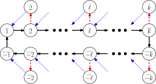
Figure 1: The turns of $\mathtt{AlgAU}$ and their transition diagram. The type AA transitions, type AF transitions, and type FA transitions are depicted by the solid (black) arrows, dashed (red) arrows, and dotted (blue) arrows, respectively.

Discouraged by this failed attempt, we followed a different approach and designed our self-stabilizing AU algorithm without a reset mechanism. Rather, we augment the $|K|$ output states with (approximately) $|K|$ “faulty states”, each one of them forms a short detour over the cyclic structure of $K$; refer to Figure 1 for the state diagram of $\mathtt{AlgAU}$, where the output states and the faulty states are marked by integers with (wide) bars and hats, respectively. Upon detecting a clock discrepancy, a node residing in an output state $s$ moves to the faulty state associated with $s$ and stays there until certain conditions are satisfied and the node may complete the faulty detour and return to a nearby output state (though, not to the original state $s$). This mechanism is designed so that clock discrepancies are resolved in a gradual “closing the gap” fashion.

The conditions that determine when a faulty node may return to an output state and the conditions for moving to a faulty state when sensing a faulty neighbor without being directly involved in a clock discrepancy are the key to the stabilization guarantees of $\mathtt{AlgAU}$. In particular, the algorithm takes a relatively cautious approach for switching between output and faulty states, that, as it turns out, allows us to avoid “vicious cycles” and ultimately bound the stabilization time as a function of $|K|=O(D)$.

2.2 Constructing the Self-Stabilizing Algorithm

The design of $\mathtt{AlgAU}$ relies upon the following definitions.

Definition (turns, able, faulty).

Fix $k=3D+2$. The states of $\mathtt{AlgAU}$, referred to hereafter as turns, are partitioned into a set $\overline{T}=\{\overline{\ell}\mid\ell\in\mathbb{Z},1\leq|\ell|\leq k\}$ of able turns and a set $\widehat{T}=\{\widehat{\ell}\mid\ell\in\mathbb{Z},2\leq|\ell|\leq k\}$ of faulty turns. A node residing in an able (resp. faulty) turn is said to be able (resp., faulty).

Definition (levels).

Throughout Sec. 2, we refer to the integers $\ell\in\mathbb{Z}$, $1\leq|\ell|\leq k$, as levels and define the level of turn $\overline{\ell}\in\overline{T}$ (resp., $\widehat{\ell}\in\widehat{T}$) to be $\ell$. We denote the level of (the turn of) a node $v\in V$ at time $t\in\mathbb{Z}_{\geq 0}$ by $\lambda_{v}^{t}$ and the set of levels sensed by $v$ at time $t$ by $\Lambda_{v}^{t}=\{\lambda_{u}^{t}\mid u\in\mathit{N}^{+}(v)\}$. For a level $\ell$, let $\mathcal{L}^{t}(\ell)=\{v\in V\mid\lambda_{v}^{t}=\ell\}$ be the set of nodes whose level at time $t$ is $\ell$. This notation is extended to level subsets $B$, defining $\mathcal{L}^{t}(B)=\bigcup_{\ell\in B}\mathcal{L}^{t}(\ell)$.

Definition (forward operator, adjacent).

For a level $\ell$, let

$$\phi(\ell)\,=\,\begin{cases}1,&\ell=-1\\ -k,&\ell=k\\ \ell+1,&\text{otherwise}\end{cases}\,.$$

Based on that, we define the forward operator $\phi^{j}(\ell)$, $j=1,2,\dots$, by setting $\phi^{1}(\ell)=\phi(\ell)$ and $\phi^{j+1}(\ell)=\phi(\phi^{j}(\ell))$. Observing that the forward operator is bijective for each $j$, we extend it to negative superscripts by setting $\phi^{-j}(\ell)=\ell^{\prime}$ if and only if $\phi^{+j}(\ell^{\prime})=\ell$. Levels $\ell$ and $\ell^{\prime}$ are said to be adjacent if either
(1) $\ell=\ell^{\prime}$;
(2) $\ell=\phi^{+1}(\ell^{\prime})$; or
(3) $\ell=\phi^{-1}(\ell^{\prime})$.

Definition (outwards operator, outwards, inwards).

Given a level $\ell$ and an integer parameter $-|\ell|<j\leq k-|\ell|$, the outwards operator $\psi^{j}(\ell)$ returns the unique level $\ell^{\prime}$ that satisfies (1) $\operatorname{sign}(\ell^{\prime})=\operatorname{sign}(\ell)$; and (2) $|\ell^{\prime}|=|\ell|+j$. This means in particular that if $j$ is positive, then $|\ell^{\prime}|>|\ell|$, and if $j$ is negative, then $|\ell^{\prime}|<|\ell|$. If $\ell^{\prime}=\psi^{j}(\ell)$ for a positive (resp., negative) $j$, then we refer to level $\ell^{\prime}$ as being $|j|$ units outwards (resp., inwards) of $\ell$.

Let $\Psi^{>}(\ell)=\left\{\psi^{j}(\ell)\mid 0<j\leq k-|\ell|\right\}$ and let $\Psi^{\geq}(\ell)=\Psi^{>}(\ell)\cup\{\ell\}$ and $\Psi^{\gg}(\ell)=\Psi^{>}(\ell)-\{\psi^{+1}(\ell)\}$. Likewise, let $\Psi^{<}(\ell)=\left\{\psi^{j}(\ell)\mid-|\ell|<j<0\right\}$ and let $\Psi^{\leq}(\ell)=\Psi^{<}(\ell)\cup\{\ell\}$ and $\Psi^{\ll}(\ell)=\Psi^{<}(\ell)-\{\psi^{-1}(\ell)\}$.

Definition (protected, good).

An edge $e=(u,v)\in E$ is said to be protected at time $t\in\mathbb{Z}_{\geq 0}$ if levels $\lambda_{v}^{t}$ and $\lambda_{u}^{t}$ are adjacent. A node $v\in V$ is said to be protected at time $t$ if all its incident edges are protected. Let $\mathit{V}_{\mathrm{p}}^{t}\subseteq V$ and $\mathit{E}_{\mathrm{p}}^{t}\subseteq E$ denote the set of nodes and edges, respectively, that are protected at time $t$. A protected node that does not sense any faulty turn is said to be good. The graph $G$ is said to be protected (resp., good) at time $t$ if all its nodes are protected (resp., good).

We are now ready to complete the description of $\mathtt{AlgAU}$. The $2k$ levels are identified with the AU clock values, associating $\phi^{+j}(\cdot)$ and $\phi^{-j}(\cdot)$ with the $+j$ and $-j$ operations, respectively, of the corresponding cyclic group. Moreover, we identify the output state set of $\mathtt{AlgAU}$ with the set $\overline{T}$ of able turns and regard the faulty turns as the remaining (non-output) states.

For the state transition function of $\mathtt{AlgAU}$, consider a node $v\in V$ residing in a turn $\nu\in\overline{T}\cup\widehat{T}$ at time $t$ and suppose that $v$ is activated at time $t$. Node $v$ remains in turn $\nu$ during step $t$ unless certain conditions on $\nu$ are satisfied, in which case, $v$ performs a state transition that belongs to one of the following three types (refer to Table 1 for a summary and to Figure 1 for an illustration):

• Suppose that $v$’s turn at time $t$ is $\nu=\overline{\ell}\in\overline{T}$, $1\leq|\ell|\leq k$. Node $v$ performs a type able-able (AA) transition in step $t$ and updates its turn to $\overline{\ell^{\prime}}\in\overline{T}$, where $\ell^{\prime}=\phi^{+1}(\ell)$, if and only if (1) $v$ is good at time $t$; and (2) $\Lambda_{v}^{t}\subseteq\{\ell,\ell^{\prime}\}$.

• Suppose that $v$’s turn at time $t$ is $\nu=\overline{\ell}\in\overline{T}$, $2\leq|\ell|\leq k$. Node $v$ performs a type able-faulty (AF) transition in step $t$ and updates its turn to $\widehat{\ell}\in\widehat{T}$ if and only if at least one of the following two conditions is satisfied: (1) $v$ is not protected at time $t$; or (2) $v$ senses turn $\widehat{\ell^{\prime}}$ at time $t$, where $\ell^{\prime}=\psi^{-1}(\ell)$.

• Suppose that $v$’s turn at time $t$ is $\nu=\widehat{\ell}\in\widehat{T}$, $2\leq|\ell|\leq k$. Node $v$ performs a type faulty-able (FA) transition in step $t$ and updates its turn to $\overline{\ell^{\prime}}\in\overline{T}$, where $\ell^{\prime}=\psi^{-1}(\ell)$ is the level one unit inwards of $\ell$, if and only if $v$ does not sense any level in $\Psi^{>}(\ell)$.

2.3 Correctness and Stabilization Time Analysis

In this section, we establish the correctness and stabilization time guarantees of $\mathtt{AlgAU}$. First, in Sec. 2.3.1, we present (and prove) certain fundamental invariants and general observations regarding the operation of $\mathtt{AlgAU}$. This allows us to prove in Sec. 2.3.2 that in the context of $\mathtt{AlgAU}$, stabilization corresponds to reaching a good graph. Following that, we focus on proving that the graph is guaranteed to become good by time $O(R(D^{3}))$. This is done in three stages, presented in Sec. 2.3.3, 2.3.4, and 2.3.5.

2.3.1 Fundamental Properties.

The following additional two definitions play a central role in the analysis of $\mathtt{AlgAU}$.

Definition (out-protected, $\ell$-out-protected).

We say that a node $v\in V$ of level $\ell$ is out-protected at time $t\in\mathbb{Z}_{\geq 0}$ if $\Lambda_{v}^{t}\cap\Psi^{\gg}(\lambda_{v}^{t})=\emptyset$. In other words, $v$ is out-protected at time $t$ if any edge $(u,v)\in E-\mathit{E}_{\mathrm{p}}^{t}$ satisfies either (1) $\operatorname{sign}(\lambda_{u}^{t})\neq\operatorname{sign}(\lambda_{v}^{t})$; or (2) $\lambda_{u}^{t}\in\Psi^{\ll}(\lambda_{v}^{t})$. Notice that the nodes in level $\ell\in\{-k,-k+1,k-1,k\}$ are always (vacuously) out-protected. Let $\mathit{V}_{\mathrm{op}}^{t}\subseteq V$ denote the set of nodes that are out-protected at time $t\in\mathbb{Z}_{\geq 0}$.

The graph $G$ is said to be out-protected at time $t\in\mathbb{Z}_{\geq 0}$ if $V=\mathit{V}_{\mathrm{op}}^{t}$. Given a level $\ell$, the graph is said to be $\ell$-out-protected at time $t$ if $\mathcal{L}^{t}\left(\Psi^{\geq}(\ell)\right)\subseteq\mathit{V}_{\mathrm{op}}^{t}$. Notice that the graph is out-protected if and only if it is both $1$-out-protected and $(-1)$-out-protected, which means that if edge $(u,v)\notin\mathit{E}_{\mathrm{p}}^{t}$, then $\operatorname{sign}(\lambda_{u}^{t})\neq\operatorname{sign}(\lambda_{v}^{t})$.

Definition (distance).

The distance between levels $\ell$ and $\ell^{\prime}$, denoted by $\operatorname{dist}(\ell,\ell^{\prime})$, is defined by the recurrence

$$\operatorname{dist}(\ell,\ell^{\prime})\,=\,\begin{cases}0,&\ell=\ell^{\prime}\\ 1+\min\{\operatorname{dist}(\ell,\phi^{-1}(\ell^{\prime})),\operatorname{dist}(\ell,\phi^{+1}(\ell^{\prime}))\},&\ell\neq\ell^{\prime}\end{cases}\,;$$

notice that this is indeed a distance function in the sense that it is symmetric and obeys the triangle inequality.

We are now ready to state the fundamental properties of $\mathtt{AlgAU}$, cast in Obs. 2.1–2.9.

Observation 2.1.

If an edge $e=(u,v)\in\mathit{E}_{\mathrm{p}}^{t}$ and $\{\lambda^{t}_{u},\lambda^{t}_{v}\}\neq\{-k,k\}$, then $e\in\mathit{E}_{\mathrm{p}}^{t+1}$.

Proof.

Consider first the case that $\lambda_{u}^{t}=\lambda_{v}^{t}=\ell$. If $\ell<0$, then $\{\lambda_{u}^{t+1},\lambda_{v}^{t+1}\}\subseteq\{\ell,\phi^{+1}(\ell)\}$, thus $e$ remains protected at time $t+1$. If $\ell>0$, then it may be the case that the level of one of the two nodes, say $u$, decreases in step $t$ due to a type FA transition so that $\lambda_{u}^{t+1}=\phi^{-1}(\ell)$. But this means that $v$ is not good at time $t$ (it has at least one faulty neighbor), hence it cannot experience a type AA transition, implying that $\lambda_{v}^{t+1}\in\{\ell,\phi^{-1}(\ell)\}$. Therefore, $e$ remains protected at time $t+1$ also in this case.

Assume now that $\lambda_{u}^{t}=\ell$ and $\lambda_{v}^{t}=\phi^{+1}(\ell)$ for a level $\ell\neq k$. Notice that $v$ cannot experience a type AA transition in step $t$ as $\ell=\phi^{-1}(\lambda_{v}^{t})\in\Lambda_{v}^{t}$. On the other hand, $u$ can experience a type FA transition only if $\ell<0$ which results in $\lambda_{u}^{t+1}=\phi^{+1}(\ell)$. Therefore, $\{\lambda_{u}^{t+1},\lambda_{v}^{t+1}\}\subseteq\{\ell,\phi^{+1}(\ell)\}$ and $e$ remains protected at time $t+1$. ∎

Observation 2.2.

If a node $v\in\mathit{V}_{\mathrm{p}}^{t}$ and $\lambda^{t}_{v}\notin\{-k,k\}$, then $v\in\mathit{V}_{\mathrm{p}}^{t+1}$.

Proof.

Follows directly from Obs. 2.1. ∎

Observation 2.3.

If a node $v\in\mathit{V}_{\mathrm{op}}^{t}$, then $v\in\mathit{V}_{\mathrm{op}}^{t+1}$.

Proof.

Follows from Obs. 2.1 by recalling that $\mathcal{L}^{t}(\ell)\subseteq\mathit{V}_{\mathrm{op}}^{t}$ for every $\ell\in\{-k,-k+1,k-1,k\}$. ∎

Observation 2.4.

For a node $v\in V$, if $\lambda_{v}^{t+1}\neq\lambda_{v}^{t}$, then $v\in\mathit{V}_{\mathrm{op}}^{t+1}$.

Proof.

Follows from Obs. 2.3 as node $v$ cannot change its level in step $t$ unless it is out-protected at time $t$. ∎

Observation 2.5.

If an edge $(u,v)\in E-\mathit{E}_{\mathrm{p}}^{t}$ with $\lambda_{u}^{t}<\lambda_{v}^{t}$, then $\lambda_{u}^{t}\leq\lambda_{u}^{t+1}<\lambda_{v}^{t+1}\leq\lambda_{v}^{t}$.

Proof.

Follows by recalling that a node that is not protected at time $t$ cannot experience a type AA transition in step $t$ and that it can experience a type FA transition in step $t$ only if it does not sense any level (strictly) outwards of its own. ∎

Observation 2.6.

If $G$ is $\ell$-out-protected at time $t$, then $G$ remains $\ell$-out-protected at time $t+1$.

Proof.

Follows from Obs. 2.3 and 2.4. ∎

Observation 2.7.

Consider a path $P$ of length $d$ between nodes $u\in V$ and $v\in V$ in $G$. If $E(P)\subseteq\mathit{E}_{\mathrm{p}}^{t}$, then $\operatorname{dist}(\lambda_{u}^{t},\lambda_{v}^{t})\leq d$.

Proof.

By induction on $d$. The assertion clearly holds if $d=0$ which implies that $u=v$. Consider a $(u,v)$-path $P$ of length $d>0$ and let $v^{\prime}$ be the node that precedes $v$ in $P$. By applying the inductive hypothesis to the $(u,v^{\prime})$-prefix of $P$, we conclude that $\operatorname{dist}(\lambda_{u}^{t},\lambda_{v^{\prime}}^{t})\leq d-1$. As $(v^{\prime},v)\in\mathit{E}_{\mathrm{p}}^{t}$, we conclude that $\operatorname{dist}(\lambda_{u}^{t},\lambda_{v}^{t})\leq\operatorname{dist}(\lambda_{u}^{t},\lambda_{v^{\prime}}^{t})+1\leq d$, thus establishing the assertion. ∎

Observation 2.8.

If $\mathit{V}_{\mathrm{p}}^{t}=V$, then there exists a level $\ell$ and an integer $0\leq d\leq D$ such that $V=\mathcal{L}^{t}\left(\left\{\phi^{+j}(\ell)\mid 0\leq j\leq d\right\}\right)$.

Proof.

Follows by applying Obs. 2.7 to the shortest paths in the graph $G$ whose lengths are at most $D$. ∎

Observation 2.9.

Consider a path $P$ of length $d$ emerging from a node $v\in V$ and assume that $E(P)\subseteq\mathit{E}_{\mathrm{p}}^{t}$ (resp., $V(P)\subseteq\mathit{V}_{\mathrm{p}}^{t}$). Fix some time $t^{\prime}\geq t$ and assume that $|\lambda_{v}^{s}|<k-d$ for every $t\leq s\leq t^{\prime}$. Then, $E(P)\subseteq\mathit{E}_{\mathrm{p}}^{t^{\prime}}$ (resp., $V(P)\subseteq\mathit{V}_{\mathrm{p}}^{t^{\prime}}$).

Proof.

Fix a time $s$. Obs. 2.7 ensures that if $E(P)\subseteq\mathit{E}_{\mathrm{p}}^{s}$ (resp., $V(P)\subseteq\mathit{V}_{\mathrm{p}}^{s}$) and $|\lambda_{v}^{s}|<k-d$, then $|\lambda_{u}^{s}|<k$ for every node $u$ in $P$. This implies that $E(P)\subseteq\mathit{E}_{\mathrm{p}}^{s+1}$ (resp., $V(P)\subseteq\mathit{V}_{\mathrm{p}}^{s+1}$) due to Obs. 2.1 (resp., Obs. 2.2). The assertion is now established by induction on $s=t,t+1,\dots,t^{\prime}-1$. ∎

2.3.2 Post-Stabilization Dynamics.

In this section, we show that the stabilization of $\mathtt{AlgAU}$ is reduced to reaching a good graph. This is stated formally in the following two lemmas.

Lemma 2.10.

If $G$ is good at time $t$, then $G$ remains good at time $t+1$.

Proof.

If all nodes are good at time $t$, then the only possible state transitions in step $t$ are of type AA. Observing that an edge $(u,v)$ with $\lambda_{u}^{t}=k$ and $\lambda_{v}^{t}=-k$ does not become non-protected via type AA transitions, we conclude by Obs. 2.1 that $\mathit{E}_{\mathrm{p}}^{t+1}=E$ and hence, $\mathit{V}_{\mathrm{p}}^{t+1}=V$. Since a type AA transition does not change the turn of a node from able to faulty, it follows that all nodes remain able at time $t+1$, hence all nodes are good at time $t+1$. ∎

Lemma 2.11.

Assume that $G$ is good at time $t$. For $i=0,1,\dots$, each node $v\in V$ experiences at least $i$ type AA transitions during the time interval $\left[t,\varrho^{D+i}(t)\right)$.

Proof.

Lem. 2.10 ensures that all nodes remain good, and in particular protected, from time $t$ onwards. For $i=0,1,\dots$, let $\tau(i)=\varrho^{i}(t)$ and let $\ell_{\min}(i)$ and $d(i)$ be the level $\ell$ and integer $d$ promised in Obs. 2.8 when applied to time $\tau(i)$. Since all nodes are good throughout the time interval $I=[\tau(i),\tau(i+1))$, it follows that every node $v\in\mathcal{L}^{\tau(i)}\left(\ell_{\min}(i)\right)$ experiences at least one type AA transition during $I$ (in particular, $v$ experiences a type AA transition upon its first activation during $I$), hence $\ell_{\min}(i+1)>\ell_{\min}(i)$. The assertion follows by Obs. 2.8 ensuring that $d(0)\leq D$. ∎

2.3.3 Towards an Out-Protected Graph.

Our goal in in the remainder of Sec. 2.3 is to establish an upper bound on the time it takes until the graph becomes good. In the current section, we make the first step towards achieving this goal by bounding the time it takes for the graph to become out-protected, starting with the following lemma.

Lemma 2.12.

Assume that $G$ is $\ell$-out-protected, $2\leq|\ell|\leq k$, at time $t$. If the turn of a node $v\in V$ at time $t$ is $\widehat{\ell}$, then $v$ experiences a type FA transition before time $\varrho^{2(k-|\ell|)+1}(t)$.

Proof.

Obs. 2.3 ensures that $v\in\mathit{V}_{\mathrm{op}}^{t^{\prime}}$ for every $t^{\prime}\geq t$. For $i=0,1,\dots$, let $\tau(i)=\varrho^{i}(t)$. We prove by induction on $k-|\ell|$ that $v$ experiences a type FA transition before time $\tau(2(k-|\ell|)+1)$, thus establishing the assertion. For the induction’s base, notice that if the turn of node $v$ at time $t$ is $\widehat{k}$ (resp., $\widehat{-k}$), then $v$ is guaranteed to experience a type FA transition, moving to state $\overline{k-1}$ (resp., $\overline{-k+1}$), upon its next activation and in particular before time $\varrho(t)=\tau(1)$.

Assume that $2\leq|\ell|\leq k-1$. If $v$ is in turn $\widehat{\ell}$ when a neighbor $u$ of $v$ in turn $\overline{\psi^{+1}(\ell)}$ is activated, then $u$ experiences a type AF transition, moving to state $\widehat{\psi^{+1}(\ell)}$. Moreover, as long as $v$ is faulty, no neighbor of $v$ can move from level $\ell$ to level $\psi^{+1}(\ell)$. Since $v$ has no neighbors in levels belonging to $\Psi^{\gg}(\ell)$ (recall that $v$ is out-protected), it follows that as long as $v$ does not experience a type FA transition, no neighbor of $v$ can move to level $\psi^{+1}(\ell)$ from another level and thus, no neighbor of $v$ can move to turn $\overline{\psi^{+1}(\ell)}$ from another turn. Therefore, it is guaranteed that at time $\tau(1)$, all neighbors $u$ of $v$ whose level satisfies $\lambda_{u}^{\tau(1)}=\psi^{+1}(\ell)$ are faulty. By the inductive hypothesis, these nodes $u$ experience a type FA transition, moving to turn $\overline{\ell}$, before time $\tau(1+2(k-|\ell|-1)+1)=\tau(2(k-|\ell|))$. In the subsequent activation of $v$, which occurs before time $\varrho(\tau(2(k-|\ell|)))=\tau(2(k-|\ell|)+1)$, $v$ experiences a type FA transition, thus establishing the assertion. ∎

Lem. 2.12 is the main ingredient in proving the following key lemma.

Lemma 2.13.

Consider an edge $(u,v)\in E-\mathit{E}_{\mathrm{p}}^{t}$ with $\lambda_{u}^{t}<\lambda_{v}^{t}$. If $G$ is $\ell$-out-protected at time $t$ for $\ell\in\{\lambda_{u}^{t},\lambda_{v}^{t}\}$, then there exists a time $t<t^{*}\leq\varrho^{2(k-|\ell|)+2}(t_{0})$ such that
(1) $\lambda_{u}^{t^{*}}\geq\lambda_{u}^{t}$;
(2) $\lambda_{v}^{t^{*}}\leq\lambda_{v}^{t}$; and
(3) at least one of the inequalities in (1) and (2) is strict.

Proof.

By Obs. 2.5, it is sufficient to prove that at least one of the two nodes $u$ and $v$ changes its level before time $\varrho^{2(k-|\ell|)+2}(t)$. Assume that the graph is $\ell$-out-protected at time $t$ for $\ell=\lambda_{v}^{t}$; the proof for the case that $\ell=\lambda_{u}^{t}$ is analogous. Let $t\leq t_{0}<\varrho(t)$ be the first time following $t$ at which $v$ is activated and based on that, define the time $t\leq t_{1}\leq\varrho(t)$ as follows: if $v$ is in turn $\widehat{\ell}$ at time $t$, then set $t_{1}=t$; otherwise ($v$ is in turn $\overline{\ell}$ at time $t$), set $t_{1}=t_{0}+1$ and notice that $v$ experiences a type AF transition in step $t_{0}$ (due to the non-protected edge $(v,v^{\prime})$) unless $v^{\prime}$ changes its level beforehand. In both cases, we know that $v$ is in turn $\widehat{\ell}$ at time $t_{1}$. Since Obs. 2.6 guarantees that the graph is $\ell$-out-protected at time $t_{1}$, we can apply Lem. 2.12 to $v$, concluding that $v$ experiences a type FA transition, and in particular changes its level, before time $\varrho^{2(k-|\ell|)+1}(t_{1})\leq\varrho^{2(k-|\ell|)+2}(t)$, thus establishing the assertion. ∎

Building on Lem. 2.13, we can now bound the time it takes for the graph to become $\ell$-out-protected after it is already $\psi^{+1}(\ell)$-out-protected.

Lemma 2.14.

Fix a level $1\leq|\ell|\leq k-1$ and assume that $G$ is $\psi^{+1}(\ell)$-out-protected at time $t$. Then, $G$ is $\ell$-out-protected at time $\varrho^{(k-|\ell|)(k-|\ell|-1)}(t)$.

Proof.

For $i=0,1,\dots$, let $\tau(i)=\varrho^{i}(t)$ and fix $t^{*}=\tau((k-|\ell|)(k-|\ell|-1))$. By Obs. 2.4, it suffices to prove that $\bigcap_{t\leq t^{\prime}\leq t^{*}}\mathcal{L}^{t^{\prime}}(\ell)\subseteq\mathit{V}_{\mathrm{op}}^{t^{*}}$. To this end, consider a node $v\in\bigcap_{t\leq t^{\prime}\leq t^{*}}\mathcal{L}^{t^{\prime}}(\ell)$ and notice that by Obs. 2.3, if $v$ is out-protected at any time $t\leq t^{\prime}\leq t^{*}$, then it remains out-protected subsequently and in particular at time $t^{*}$. Moreover, Obs. 2.1 ensures that any neighbor of $v$ whose level at time $t$ belongs to $\Psi^{\leq}(\ell)\cup\{\psi^{+1}(\ell)\}$ cannot move to a level in $\Psi^{\gg}(\ell)$ as long as $v$ is in level $\ell$.

So, it remains to consider a neighbor $u\in\mathit{N}(v)$ of $v$ with $\lambda_{u}^{t}\in\Psi^{\gg}(\ell)$ and show that the level of $u$ moves inwards and becomes adjacent to $\ell$ by time $t^{*}$; indeed, Obs. 2.1 ensures that once $u$ reaches a level adjacent to $\ell$, it cannot move back to a level in $\Psi^{\gg}(\ell)$ unless $v$ leaves level $\ell$. To this end, we define

$$\textstyle f(\ell^{*})\,=\,\sum_{j=|\ell|+2}^{|\ell^{*}|}(2(k-j)+2)$$

and prove that if $\lambda_{u}^{t}=\ell^{*}\in\Psi^{\gg}(\ell)$, then $u$ reaches level $\psi^{+1}(\ell)$ by time $\tau(f(\ell^{*}))$. The assertion is established by observing that $f(k)=(k-|\ell|)(k-|\ell|-1)$.

Since the graph $G$ is $\psi^{+1}(\ell)$-out-protected at time $t$, Obs. 2.6 guarantees that $G$ is $\psi^{+1}(\ell)$-out-protected at all times subsequent to $t$ and hence, also $\ell^{\prime}$-out-protected for every $\ell^{\prime}\in\Psi^{>}(\ell)$. Therefore, we can repeatedly apply Lem. 2.13 to edge $(u,v)$ and conclude by induction on $\ell^{\prime}$ that $u$ moves from level $\ell^{\prime}\in\Psi^{\gg}(\ell)$, $|\ell^{\prime}|\leq\ell^{*}$, to level $\psi^{-1}(\ell^{\prime})$ by time

$$\textstyle\tau\left(\sum_{j=|\ell^{\prime}|}^{|\ell^{*}|}(2(k-j)+2)\right)\,.$$

The proof is then completed by plugging $\ell^{\prime}=\psi^{+2}(\ell)$. ∎

Since the graph $G$ is $\ell$-out-protected for $\ell\in\{-k,-k+1,k-1,k\}$ already at time $0$ and since being $1$-out-protected and ($-1$)-out-protected implies that $G$ is out-protected, Lem. 2.14 yields the following corollary.

Corollary 2.15.

There exists a time $T_{0}\leq R(O(k^{3}))$ such that $G$ is out-protected at all times $t\geq T_{0}$.

2.3.4 From an Out-Protected to a Justified Graph.

In what follows, we take $T_{0}$ to be the time promised in Corollary 2.15 and consider the execution from time $T_{0}$ onwards.

Definition (justifiably faulty, unjustifiably faulty, justified).

A node $v\in V$ whose turn at time $t$ is $\widehat{\ell}$, $2\leq|\ell|\leq k$, is said to be justifiably faulty if either (1) $v\notin\mathit{V}_{\mathrm{p}}^{t}$; or (2) $v$ admits a neighbor whose turn at time $t$ is $\widehat{\psi^{-1}(\ell)}$. A faulty node that is not justifiably faulty is said to be unjustifiably faulty. We say that the graph $G$ is justified if it does not admit any unjustifiably faulty node.

A key feature of $\mathtt{AlgAU}$ is that nodes do not become unjustifiably faulty once the graph is out-protected.

Lemma 2.16.

If a node $v\in V$ is not unjustifiably faulty at time $t\geq T_{0}$, then $v$ is not unjustifiably faulty at time $t+1$.

Proof.

Assume that node $v$ is either (1) able at time $t$ and experiences a type AF transition in step $t$; or (2) justifiably faulty at time $t$ (and remains faulty at time $t+1$). In both cases, we know that $v$ admits a neighboring node $u\in\mathit{N}(v)$ that satisfies at least one of the following two conditions: (i) $\lambda_{u}^{t}$ is not adjacent to $\lambda_{v}^{t}$; or (ii) $\lambda_{u}^{t}=\psi^{-1}(\lambda_{v}^{t})$ and $u$ is faulty at time $t$.

Assuming that condition (i) holds, we know that $\operatorname{sign}(\lambda_{u}^{t})\neq\operatorname{sign}(\lambda_{v}^{t})$ as $G$ is out-protected at time $t$. Since $v$ is faulty at time $t+1$, it follows that $\lambda_{v}^{t+1}=\lambda_{v}^{t}$ with $|\lambda_{v}^{t+1}|\geq 2$. Thus, $\operatorname{sign}(\lambda_{u}^{t+1})=\operatorname{sign}(\lambda_{u}^{t})$ and edge $(u,v)$ remains non-protected at time $t+1$. Assuming that condition (ii) holds, node $u$ cannot experience a type FA transition in step $t$ as $\lambda_{v}^{t}=\psi^{+1}(\lambda_{u}^{t})\in\Lambda_{u}^{t}$, thus it remains faulty at time $t+1$. Therefore, we conclude that $v$ is justifiably faulty at time $t+1$. ∎

Corollary 2.17 is now derived by combining Corollary 2.15 and Lem. 2.16, recalling that Lem. 2.12 ensures that if the graph is out-protected at time $T_{0}$, then any (justifiably or) unjustifiably faulty node experiences a type FA transition, and in particular stops being unjustifiably faulty, before time $\varrho^{O(k)}(T_{0})\leq R(O(k^{3}))$.

Corollary 2.17.

There exists a time $T_{0}\leq T_{1}\leq R(O(k^{3}))$ such that $G$ is justified at all times $t\geq T_{1}$.

2.3.5 From a Justified to a Good Graph.

In what follows, we take $T_{1}$ to be the time promised in Corollary 2.17 and consider the execution from time $T_{1}$ onwards. In the current section, we complete the analysis by up-bounding the time it takes for the graph to become good following time $T_{1}$, starting with the following lemma.

Lemma 2.18.

If $G$ is protected at time $t\geq T_{1}$, then $G$ is good at time $t$.

Proof.

Assume by contradiction that the graph admits faulty nodes at time $t$ and among these nodes, let $v\in V$ be a node that minimizes $|\lambda_{v}^{t}|$. Since $t\geq T_{1}$, Corollary 2.17 ensures that $v$ is justifiably faulty at time $t$. The assumption that $G$ is protected implies that $v$ admits a neighbor $u\in\mathit{N}(v)$ whose turn at time $t$ is $\widehat{\psi^{-1}(\lambda_{v}^{t})}$, in contradiction to the choice of $v$. ∎

Owing to Lem. 2.18, our goal in the remainder of this section is to prove that it does not take too long after time $T_{1}$ for the graph to become protected. Lem. 2.19 plays a key role in in achieving this goal.

Lemma 2.19.

If a node $v\in V-\mathit{V}_{\mathrm{p}}^{t}$ for some time $t\geq T_{1}$, then there exists a time $t\leq t^{\prime}\leq\varrho^{k(k-1)}(t)$ such that $v\in\mathit{V}_{\mathrm{p}}^{t^{\prime}}$ with $\lambda_{v}^{t^{\prime}}\in\{-1,1\}$.

Proof.

Since the graph is out-protected at all times after $T_{1}\geq T_{0}$, it follows that if edge $(v,v^{\prime})\in E-\mathit{E}_{\mathrm{p}}^{t}$, then (1) $\operatorname{sign}(\lambda_{v}^{t})\neq\operatorname{sign}(\lambda_{v^{\prime}}^{t})$; and (2) $\operatorname{dist}(\lambda_{v}^{t},\lambda_{v^{\prime}}^{t})\geq 2$. Obs. 2.5 and Lem. 2.13 guarantee that the levels of $v$ and $v^{\prime}$ move inwards until they meet with $\{\lambda_{v}^{t^{\prime}},\lambda_{v^{\prime}}^{t^{\prime}}\}=\{-1,1\}$ at some time $t\leq t^{\prime}\leq\varrho^{z}(t)$ for $z=\sum_{j=2}^{k}2(k-j)+2=k(k-1)$. The assertion follows as this is true for all edges $(v,v^{\prime})\in E-\mathit{E}_{\mathrm{p}}^{t}$. ∎

Lem. 2.19 by itself does not complete the analysis as it does not address protected nodes that become non-protected (alas, still out-protected). The following lemma provides a sufficient condition for the whole graph to become protected.

Lemma 2.20.

Consider a node $v\in V$ and assume that there exist times $T_{1}\leq t<t^{\prime}$ such that (i) $\lambda_{v}^{t}=1$; and (ii) $\lambda_{v}^{t^{\prime}}=2D+2$. Then $G$ is protected at time $t^{\prime}$.

Proof.

By Lem. 2.10 and 2.18, if all nodes are protected at some time after time $T_{1}$, then all nodes remain (good and hence) protected indefinitely. Therefore, we establish the assertion by proving the following claim and plugging $d=D$: Assume that there exist levels $1\leq\ell<\ell^{\prime}\leq 2D+2$ with $\ell^{\prime}-\ell=2d+1$ such that
(I) $v$ moves in step $t$ from level $\lambda_{v}^{t}=\ell$ to level $\lambda_{v}^{t+1}=\ell+1$;
(II) $v$ moves in step $t^{\prime}-1$ from level $\lambda_{v}^{t^{\prime}-1}=\ell^{\prime}-1$ to level $\lambda_{v}^{t^{\prime}}=\ell^{\prime}$; and
(III) $\ell<\lambda_{v}^{s}<\ell^{\prime}$ for all $t<s<t^{\prime}$.
Then all nodes at distance at most $d$ from $v$ are protected at time $t^{\prime}$.

Node $v$ can move from level $\ell$ to level $\ell+1$ in step $t$ only if it experiences a type AA transition, which requires $v$ to be protected at time $t$. By Obs. 2.2, $v$ remains protected throughout the time interval $[t,t^{\prime}]$.

We prove that all other nodes in $B(v,d)=\{u\in V\mid\operatorname{dist}_{G}(u,v)\leq d\}$ are protected at time $t^{\prime}$ by induction on $d$. The assertion holds trivially for $d=0$ as $B(v,0)=\{v\}$. Assume that the assertion holds for $d-1\geq 0$ and consider a node $u\in B(v,d)$. Let $P$ be a shortest $(v,u)$-path in $G$ and let $w$ be the node succeeding $v$ along $P$.

Since $v$ experiences $2d+1$ type AA transitions while moving from level $\ell$ to level $\ell^{\prime}$ during the time interval $[t,t^{\prime}]$, there must exist times $t<t_{w}\leq t^{\prime}_{w}<t^{\prime}$ such that
(I) $w$ moves in step $t_{w}$ from level $\lambda_{w}^{t_{w}}=\ell+1$ to level $\lambda_{w}^{t_{w}+1}=\ell+2$;
(II) $w$ moves in step $t^{\prime}_{w}-1$ from level $\lambda_{w}^{t^{\prime}_{w}-1}=\ell^{\prime}-2$ to level $\lambda_{w}^{t^{\prime}_{w}}=\ell^{\prime}-1$; and
(III) $\ell+1<\lambda_{w}^{s}<\ell^{\prime}-1$ for all $t_{w}<s<t^{\prime}_{w}$.
By the inductive hypothesis, all nodes in $B(u,d-1)$, and in particular the nodes along the $(w,u)$-suffix of $P$, are protected at time $t^{\prime}_{w}$, hence all nodes in $P$ are protected at time $t<t^{\prime}_{w}<t^{\prime}$. Recalling that $1\leq\ell<\lambda_{v}^{s}\leq\ell^{\prime}\leq 2D+2$ for all $t^{\prime}_{w}\leq s\leq t^{\prime}$, we employ Obs. 2.9 to conclude that all nodes in $P$ are protected at time $t^{\prime}$, thus establishing the assertion. ∎

Lem. 2.20 allows us to establish Lem. 2.21 for which we need the following additional definition.

Definition (grounded).

A path $P$ of length at most $D$ in $G$ is said to be grounded at time $t$ if (1) $V(P)\subseteq\mathit{V}_{\mathrm{p}}^{t}$; and (2) $P$ has an endpoint $u$ satisfying $\lambda_{u}^{t}\in\{-1,1\}$. A node $v\in V$ is said to be grounded at time $t$ if it belongs to a grounded path.

Lemma 2.21.

If a node $v\in V$ is grounded at time $t\geq T_{1}$, then $v\in\mathit{V}_{\mathrm{p}}^{t^{\prime}}$ for all $t^{\prime}\geq t$.

Proof.

The fact that node $v$ is grounded at time $t$ means in particular that $v\in\mathit{V}_{\mathrm{p}}^{t}$ so assume by contradiction that $v\notin\mathit{V}_{\mathrm{p}}^{t^{\prime}}$ for a time $t^{\prime}>t$. Consider the path $P$ of length at most $D$ due to which $v$ is grounded at time $t$ and let $u$ be the endpoint of $P$ that satisfies $\lambda_{u}^{t}\in\{-1,1\}$. Since $V(P)\subseteq\mathit{V}_{\mathrm{p}}^{t}$, we can apply Obs. 2.9 to $P$ and $u$, concluding that there exists a time $t<s\leq t^{\prime}$ such that $|\lambda_{u}^{s}|\geq k-D$. Since $u$ moves from level $\lambda_{u}^{t}\in\{-1,1\}$ to level $\lambda_{u}^{s}$ satisfying $|\lambda_{u}^{s}|\geq k-D=2D+2$ during the time interval $[t,s)$, it follows that there exist times $t\leq r<r^{\prime}\leq s$ such that $u$ moves from level $\lambda_{u}^{r}=1$ up to level $\lambda_{u}^{r^{\prime}}=2D+2$ during the time interval $[r,r^{\prime})$. Employing Lem. 2.20, we conclude that $G$ is protected from time $r^{\prime}$ onwards, which contradicts the assumption that $v\notin\mathit{V}_{\mathrm{p}}^{t^{\prime}}$ as $t^{\prime}\geq s\geq r^{\prime}$. ∎

We are now ready to prove the following lemma that, when combined with Lem. 2.10, 2.11, and 2.18, establishes Thm. 1.1 as $k=O(D)$.

Lemma 2.22.

There exists a time $T_{1}\leq T_{2}\leq R(O(k^{3}))$ such that $G$ is protected at time $T_{2}$.

Proof.

Fix a node $v\in V$. In the context of this proof, we say that $v$ is post-grounded at time $t$ if $v$ was grounded at some time $T_{1}\leq t^{\prime}\leq t$. By Lem. 2.21, it suffices to prove that $v$ becomes post-grounded by time $R(O(k^{3}))$. In fact, since graph $G$ is out-protected after time $T_{1}\geq T_{0}$ and since in an out-protected graph, a non-protected node becomes protected if and only if it becomes grounded, it follows that $G$ becomes protected exactly when all its nodes become post-grounded.

For $t\geq T_{1}$, let $G_{\mathrm{p}}^{t}=(V,\mathit{E}_{\mathrm{p}}^{t})$. Assuming that $G$ is still not protected at time $t$ (i.e., that $\mathit{V}_{\mathrm{p}}^{t}\subsetneq V$), let $x^{t}$ be a node $x\in V-\mathit{V}_{\mathrm{p}}^{t}$ that minimizes $\operatorname{dist}_{G_{\mathrm{p}}^{t}}(v,x)$, and among those, a node that minimizes $|\lambda_{x}^{t}|$ (breaking the remaining ties in an arbitrary consistent manner). Notice that although we cannot bound the diameter of $G_{\mathrm{p}}^{t}$, the choice of $x^{t}$ implies that $d^{t}=\operatorname{dist}_{G_{\mathrm{p}}^{t}}(v,x^{t})\leq D$. Let $P^{t}$ be a $(v,x^{t})$-path in $G_{\mathrm{p}}^{t}$ that realizes $d^{t}$.

The choice of $x^{t}$ and $P^{t}$ ensures that $x^{t}\notin\mathit{V}_{\mathrm{p}}^{t}$ and that $V(P^{t})-\{x^{t}\}\subseteq\mathit{V}_{\mathrm{p}}^{t}$. If a node $u\in V(P^{t})-\{x^{t}\}$ becomes non-protected in step $t$, then $d^{t+1}\leq\operatorname{dist}_{G_{\mathrm{p}}^{t}}(v,u)<\operatorname{dist}_{G_{\mathrm{p}}^{t}}(v,x^{t})=d^{t}$. Moreover, if $x^{t}$ remains non-protected at time $t+1$, then $d^{t+1}\leq d^{t}$. The more interesting case occurs when $V(P^{t})-\{x^{t}\}\subseteq\mathit{V}_{\mathrm{p}}^{t+1}$ and $x^{t}$ also becomes protected in step $t$ which means that all nodes in $P^{t}$ are protected at time $t+1$. Recalling that the graph is out-protected after time $T_{1}\geq T_{0}$, we know that $\lambda_{x^{t}}^{t+1}\in\{-1,1\}$, hence $P^{t}$ is grounded at time $t+1$ and $v$ is post-grounded from time $t+1$ onwards.

To complete the proof, let $\tau(i)=\varrho^{i}(T_{1})$ for $i=0,1,\dots$ and notice that Lem. 2.19 guarantees that if $G$ is still not protected at time $\tau(i)$, then $x^{\tau(i)}$ becomes protected before time $\tau(i+O(k^{2}))$. Therefore, if node $v$ is still not post-grounded at time $\tau(i)$, then either (1) $v$ is post-grounded at time $\tau(i+O(k^{2}))$; or (2) $d^{\tau(i+O(k^{2}))}<d^{\tau(i)}$. As $0\leq d^{t}\leq D$ for all $t\geq T_{1}$, we conclude that node $v$ must become post-grounded by time $\tau(O(D\cdot k^{2}))=\tau(O(k^{3}))$. ∎

3 Algorithms for LE and MIS

In this section, we present the synchronous algorithms promised in Thm. 1.3 and 1.4. Specifically, our MIS algorithm, denoted by $\mathtt{AlgMIS}$, is developed in Sec. 3.1, and our LE algorithm, denoted by $\mathtt{AlgLE}$, is developed in Sec. 3.2.

A common key ingredient in the design of $\mathtt{AlgMIS}$ and $\mathtt{AlgLE}$ is a (synchronous) module denoted by $\mathtt{Restart}$. This module is invoked upon detecting an illegal configuration and, as its name implies, resets all other modules, allowing the algorithm a “fresh start” from a uniform initial configuration, that is, a configuration in which all nodes share the same initial state $q^{*}_{0}$, chosen by the algorithm designer. Module $\mathtt{Restart}$ consists of $O(D)$ states, among them are two designated states denoted by $\mathtt{Restart}$-entry and $\mathtt{Restart}$-exit: a node enters $\mathtt{Restart}$ by moving from a non-$\mathtt{Restart}$ state to $\mathtt{Restart}$-entry; a node exits $\mathtt{Restart}$ by moving from $\mathtt{Restart}$-exit to the initial state $q^{*}_{0}$. The main guarantee of $\mathtt{Restart}$ is cast in the following theorem.

Theorem 3.1.

If some node is in a $\mathtt{Restart}$ state at time $t_{0}$, then there exists a time $t_{0}\leq t\leq t_{0}+O(D)$ such that all nodes exit $\mathtt{Restart}$, concurrently, in step $t$.

A module that satisfies the promise of Thm. 3.1 is developed by Boulinier et al. [BPV05]. Due to some differences between the computational model used in the current paper and the one used in [BPV05], we provide a standalone implementation (and analysis) of module $\mathtt{Restart}$ in Sec. 3.3, relying on algorithmic principles similar to those used by Boulinier et al.

3.1 Algorithm $\mathtt{AlgMIS}$

For clarity of the exposition, the MIS algorithm $\mathtt{AlgMIS}$ is presented in a procedural style; converting it to a randomized state machine with $O(D)$ states is straightforward. The algorithm is designed assuming that the execution starts concurrently at all nodes; this assumption is plausible due to Thm. 3.1 and given the algorithm’s fault detection guarantees (described in the sequel). Throughout, we say that a node $v\in V$ is decided if $v$ resides in an output state; otherwise, we say that $v$ is undecided. An edge is said to be decided if at least one of its endpoints is decided, and undecided if both its endpoints are undecided. Recall that in the context of the MIS problem, the output value of a decided node $v$ is $1$ (resp., $0$) if $v$ is included in (resp., excluded from) the constructed MIS; we subsequently denote by $\mathit{IN}$ (resp., $\mathit{OUT}$) the set of decided nodes with output $1$ (resp, $0$).

The algorithm consists of three modules, denoted by $\mathtt{RandPhase}$, $\mathtt{DetectMIS}$, and $\mathtt{Compete}$; all nodes participate in $\mathtt{RandPhase}$, whereas $\mathtt{DetectMIS}$ involves only the decided nodes and $\mathtt{Compete}$ involves only the undecided nodes. Module $\mathtt{RandPhase}$ runs indefinitely and divides the execution into phases so that for each phase $\pi$, (1) all nodes start (and finish) $\pi$ concurrently; and (2) the length (in rounds) of $\pi$ is $D+O(\log n)$ in expectation and whp.

The role of $\mathtt{DetectMIS}$ is to detect local faults among the decided nodes, namely, two neighboring $\mathit{IN}$ nodes or an $\mathit{OUT}$ node with no neighboring $\mathit{IN}$ node. The module runs indefinitely (over the decided nodes) and is designed so that a local fault is detected in each round (independently) with a positive constant probability, which means that no local fault remains undetected for more than $O(\log n)$ rounds whp. Upon detecting a local fault, $\mathtt{DetectMIS}$ invokes module $\mathtt{Restart}$ and the execution of $\mathtt{AlgMIS}$ starts from scratch once $\mathtt{Restart}$ is exited.

Module $\mathtt{Compete}$ is invoked from scratch in each phase, governing the competition of the undecided nodes over the “privilege” to be included in the constructed MIS. Taking $U\subseteq V$ to be the set of undecided nodes at the beginning of a phase $\pi$ and taking $G(U)$ to denote the subgraph induced on $G$ by $U$, module $\mathtt{Compete}$ assigns (implicitly) a random variable $Z(u)\in\mathbb{Z}_{\geq 0}$ to each node $u\in U$ so that the following three properties are satisfied:
(1) $\mathbb{P}\left(\bigwedge_{w\in W}[Z(u)>Z(w)]\right)\geq\Omega\left(\frac{1}{|W|+1}\right)$ for every node subset $W\subseteq U-\{u\}$;
(2) if $Z(u)>Z(w)$ for all nodes $w\in\mathit{N}_{G(U)}(u)$, then $u$ joins $\mathit{IN}$; and
(3) $u$ joins $\mathit{OUT}$ during $\pi$ if and only if node $v$ joins $\mathit{IN}$ for some $v\in\mathit{N}_{G(U)}(u)$ whp.

It is well known (see, e.g., [ABI86, MRSZ11, EW13]) that properties (1)–(3) ensure that in expectation, a (positive) constant fraction of the undecided edges become decided during $\pi$. Using standard probabilistic arguments, we deduce that all edges become decided within $O(\log n)$ phases in expectation and whp, thus, by applying properties (1) and (2) to the nodes of degree $\operatorname{deg}_{G(U)}(v)=0$, all nodes become decided within $O(\log n)$ phases in expectation and whp. Thm. 1.4 follows, again, by standard probabilistic arguments. We now turn to present the implementation of the three modules.

3.1.1 Implementing Module $\mathtt{RandPhase}$.

As discussed earlier, module $\mathtt{RandPhase}$ divides the execution into phases. Each phase consists of a (random) prefix of length $X$ and a (deterministic) suffix of length $D+2$, where $X$ is a random variable that satisfies (1) $X\leq O(\log n)$ in expectation and whp; and (2) $X\geq c_{0}\log n$ whp for a constant $c_{0}>0$ that can be made arbitrarily large. The module is designed so that if all nodes start a phase $\pi$ concurrently, then all nodes finish $\pi$ (and start the next phase) concurrently after $D+2+X$ rounds (this guarantee holds with probability $1$).

To implement $\mathtt{RandPhase}$, each node $v\in V$ maintains two variables, denoted by $v.\mathtt{flag}\in\{0,1\}$ and $v.\mathtt{step}\in\{0,1,\dots,D+2\}$; the former variable controls the length of the phase’s random prefix, whereas the latter is used to ensure that all nodes finish the phase concurrently, exactly $D+2$ rounds after the random prefix is over (for all nodes).

To this end, when a phase begins, $v$ sets $v.\mathtt{step}\leftarrow 0$ and $v.\mathtt{flag}\leftarrow 1$. As long as $v.\mathtt{flag}=1$, node $v$ tosses a (biased) coin and resets $v.\mathtt{flag}\leftarrow 0$ with probability $0<p_{0}<1$, where $p_{0}=p_{0}(c_{0})$ is a constant determined by $c_{0}$. Once $v.\mathtt{flag}=0$, the actions of $v$ become deterministic: Let $v.\mathtt{step}_{\min}=\min\{u.\mathtt{step}:u\in\mathit{N}^{+}(v)\}$. If $v.\mathtt{step}_{\min}<D+2$, then $v$ sets $v.\mathtt{step}\leftarrow\mathtt{step}_{\min}+1$; otherwise ($v.\mathtt{step}_{\min}=D+2$), the phase ends and a new phase begins. On top of these rules, if, at any stage of the execution, $v$ senses a node $u\in\mathit{N}^{+}(v)$ for which $|u.\mathtt{step}-v.\mathtt{step}|>1$, then $v$ invokes module $\mathtt{Restart}$.

To analyze $\mathtt{RandPhase}$, consider a phase $\pi$ that starts concurrently for all nodes and let $X_{v}$ be the number of rounds in which node $v\in V$ kept $v.\mathtt{flag}=1$ since $\pi$ began, observing that $X_{v}$ is a $\mathrm{Geom}(p_{0})$ random variable. Since the random variables $X_{v}$, $v\in V$, are independent, we can apply Obs. 3.2, established by standard probabilistic arguments, to conclude that the random variable $X=\max_{v\in V}X_{v}$ satisfies (1) $X\leq O(\log n)$ in expectation and whp; and (2) $X\geq c_{0}\log n$ whp, where the relation between $c_{0}$ and $p_{0}$ is derived from Obs. 3.2.

Observation 3.2.

Fix some constant $0<p\leq 1/2$ and let $Y_{1},\dots,Y_{n}$ be $n$ independent and identically distributed $\mathrm{Geom}(p)$ random variables. Then, the random variable $Y=\max_{i\in[n]}Y_{i}$ satisfies (1) $Y\leq O(\log n)$ in expectation and whp; and (2) $Y\geq c\log n$ whp for any constant $c<\ln(2)/(2p)$.

To complete the analysis of $\mathtt{RandPhase}$, we introduce the following notation and terminology. Given a node $v\in V$, let $v.\mathtt{step}^{t}$ and $v.\mathtt{step}_{\min}^{t}$ denote the values of $v.\mathtt{step}$ and $v.\mathtt{step}_{\min}$, respectively, at time $t$. An edge $e=\{u,v\}\in E$ is said to be valid at time $t$, if $|u.\mathtt{step}^{t}-v.\mathtt{step}^{t}|\leq 1$. Let $v_{\max}$ be a node $v\in V$ that realizes $X_{v}=X$. We can now establish the following two observations.

Observation 3.3.

If all edges are valid at time $t$, then $|u.\mathtt{step}^{t}-v.\mathtt{step}^{t}|\leq\operatorname{dist}_{G}(u,v)$ for every two nodes $u,v\in V$.

Proof.

Follows by a straightforward induction on $\operatorname{dist}_{G}(u,v)$. ∎

Observation 3.4.

As long as $v_{\max}.\mathtt{step}=0$, all edges are valid and $v.\mathtt{step}\leq D$ for all nodes $v\in V$.

Proof.

The assertion clearly holds when the phase begins and $v.\mathtt{step}=0$ for all nodes $v\in V$. Obs. 3.3 ensures that if all edges are valid at time $t$ and $v_{\max}.\mathtt{step}^{t}=0$, then $\max_{v\in V}v.\mathtt{step}^{t}\leq D$. The assertion follows as $\mathtt{RandPhase}$ can invalidate a valid edge $\{u,v\}$ only if $u.\mathtt{step}=v.\mathtt{step}=D+2>D$. ∎

Based on Obs. 3.3 and 3.4, we can prove the following key lemma.

Lemma 3.5.

Suppose that node $v_{\max}$ resets $v_{\max}.\mathtt{flag}\leftarrow 0$ in round $t$. Then, the following three conditions are satisfied for every $0\leq d\leq D$:
(1) all edges are valid at time $t+d$;
(2) $v.\mathtt{step}^{t+d}\geq d$ for every node $v\in V$; and
(3) $v.\mathtt{step}^{t+d}\leq\max\{d,\operatorname{dist}_{G}(v_{\max},v)\}$ for every node $v\in V$.

Proof.

By induction on $d=0,1,\dots,D$. The base case holds by Obs. 3.4 as $v_{\max}.\mathtt{step}^{t}=0$, so assume that the assertion holds for $d-1$ and consider the situation at time $t+d$. The inductive hypothesis ensures that all edges are valid at time $t-d-1$ and that $\max_{v\in V}v.\mathtt{step}^{t-d-1}\leq D$, hence all edges remain valid at time $t+d$, establishing condition (1).

To show that condition (2) holds, consider some node $v\in V$. The inductive hypothesis ensures that $d-1\leq v.\mathtt{step}_{\min}^{t+d-1}\leq D$, hence $v.\mathtt{step}^{t+d}=v.\mathtt{step}_{\min}^{t+d-1}+1\geq d$, establishing condition (2).

For condition (3), consider some node $v\in V$ and assume first that $\operatorname{dist}_{G}(v_{\max},v)\leq d-1$. The inductive hypothesis ensures that $v.\mathtt{step}^{t+d-1}=d-1$, hence $v.\mathtt{step}_{\min}^{t+d-1}=d-1$ implying that $v.\mathtt{step}$ is incremented in round $t+d-1$ from $v.\mathtt{step}^{t+d-1}=d-1$ to $v.\mathtt{step}^{t+d}=d=\max\{d,\operatorname{dist}_{G}(v_{\max},v)\}$. Now, consider the case that $\operatorname{dist}_{G}(v_{\max},v)=d$ and let $u$ be the node that precedes $v$ along a shortest $(v_{\max},v)$-path in $G$. Since $\operatorname{dist}_{G}(v_{\max},u)=d-1$, we know that $u.\mathtt{step}$ is incremented in round $t+d-1$ from $u.\mathtt{step}^{t+d-1}=d-1$ to $u.\mathtt{step}^{t+d}=d$. This implies that $v.\mathtt{step}_{\min}^{t+d-1}\leq d-1$, thus $v.\mathtt{step}^{t+d}\leq d=\max\{d,\operatorname{dist}_{G}(v_{\max},v)\}$.

We can now prove by a secondary induction on $\delta=d,d+1,\dots,D$ that $v.\mathtt{step}^{t+d}\leq\operatorname{dist}_{G}(v_{\max},v)=\max\{d,\operatorname{dist}_{G}(v_{\max},v)\}$ for every node $v\in V$ with $\operatorname{dist}_{G}(v_{\max},v)=\delta$, thus establishing condition (3). The base case ($\delta=d$) of the secondary induction has already bean established, so assume that it holds for $\delta$ and consider a node $v\in V$ with $\operatorname{dist}_{G}(v_{\max},v)=\delta+1$. Let $u$ be the node that precedes $v$ along a shortest $(v_{\max},v)$-path in $G$. Since $\operatorname{dist}_{G}(v_{\max},u)=\delta$, we can apply the secondary inductive hypothesis, concluding that $u.\mathtt{step}^{t+d}\leq\operatorname{dist}_{G}(v_{\max},u)$. As edge $\{u,v\}$ is valid at time $t+d$, we conclude by Obs. 3.3 that $v.\mathtt{step}^{t+d}\leq u.\mathtt{step}^{t+d}+1\leq\operatorname{dist}_{G}(v_{\max},u)+1=\operatorname{dist}_{G}(v_{\max},v)$, establishing the step of the secondary induction. ∎

By plugging $d=D$ into Lem. 3.5, we obtain the following corollary.

Corollary 3.6.

Suppose that node $v_{\max}$ resets $v_{\max}.\mathtt{flag}\leftarrow 0$ in round $t$. Then, all nodes $v\in V$
(1) set $v.\mathtt{step}\leftarrow D+1$ concurrently in round $t+D$;
(2) set $v.\mathtt{step}\leftarrow D+2$ concurrently in round $t+D+1$; and
(3) start the next phase concurrently in round $t+D+2$.

3.1.2 Implementing Module $\mathtt{Compete}$.

Consider the execution of module $\mathtt{Compete}$ in a phase $\pi$ and let $U\subseteq V$ be the set of nodes that are still undecided at the beginning of $\pi$. The implementation of $\mathtt{Compete}$ is based on a binary variable, denoted by $v.\mathtt{candidate}\in\{0,1\}$, that each node $v\in U$ maintains, indicating that $v$ is still a candidate to join $\mathit{IN}$ during $\pi$. When $\pi$ begins, $v$ sets $v.\mathtt{candidate}\leftarrow 1$; then, $v$ proceeds by participating in a sequence of random trials that continues as long as $v.\mathtt{candidate}=1$ and $v.\mathtt{step}\leq D$ (recall that $v.\mathtt{step}$ is the variable that controls the deterministic suffix of module $\mathtt{RandPhase}$). Each trial consists of two rounds: in the first round, $v$ tosses a fair coin, denoted by $C_{v}\in_{r}\{0,1\}$; in the second round, $v$ computes the indicator $I_{C}=\bigvee_{u\in\mathit{N}^{+}_{G(U)}(v)\,:\,u.\mathtt{candidate}=1}C_{u}$. If $C_{v}=0$ and $I_{C}=1$, then $v$ resets $v.\mathtt{candidate}\leftarrow 0$; otherwise, $v.\mathtt{candidate}$ remains $1$.

If $v.\mathtt{candidate}$ is still $1$ when $v.\mathtt{step}$ is incremented to $v.\mathtt{step}\leftarrow D+1$, then $v$ joins $\mathit{IN}$. This is sensed in the subsequent round by $v$’s undecided neighbors that join $\mathit{OUT}$ in response. Notice that by Corollary 3.6, all nodes increment the $\mathtt{step}$ variables concurrently to $D+1$ and then to $D+2$, hence nodes may join $\mathit{IN}$ and $\mathit{OUT}$ only during the penultimate and ultimate rounds, respectively, of phase $\pi$.

We now turn to analyze $\mathtt{Compete}$ during phase $\pi$. Assume for the sake of the analysis that a node $v\in U$ keeps on participating in the trials in a “vacuous” manner, tossing the $C_{v}$ coins in vain, even after $v.\mathtt{candidate}\leftarrow 0$, until $v.\mathtt{step}\leftarrow D+1$; this has no influence on the nodes that truly participate in the trials as the trials’ outcome is not influenced by any node $v\in U$ with $v.\mathtt{candidate}=0$.

Recall that the guarantees of $\mathtt{RandPhase}$ ensure that at least $c_{0}\log n$ rounds have elapsed in phase $\pi$ whp before node $v_{\max}$ resets $v_{\max}.\mathtt{flag}\leftarrow 0$, where $c_{0}$ is an arbitrarily large constant; condition hereafter on this event. Moreover, $v_{\max}$ starts to increment variable $v_{\max}.\mathtt{step}$ only after $v_{\max}.\mathtt{flag}\leftarrow 0$. Therefore, when a node $v\in U$ sets $v.\mathtt{step}\leftarrow D+1$, we know that at least $c_{0}\log n$ rounds have already elapsed in phase $\pi$ which means that the undecided nodes participate in at least $\tau=\lfloor c_{0}/2\rfloor\log n$ trials during $\pi$.

For a node $v\in U$, let $C_{v}^{i}$ denote the value of the coin $C_{v}$ tossed by $v$ in trial $i=1,\dots,\tau$. Let $v.\mathtt{candidate}^{i}$ denote the value of the variable $v.\mathtt{candidate}$ at the beginning of trial $i=1,\dots,\tau$ and based on that, define the random variable $Z(v)=\sum_{i=1}^{\tau}2^{\tau-i}\cdot C_{v}^{i}$. Module $\mathtt{Compete}$ is designed so that a node $v\in V$ with $v.\mathtt{candidate}^{i}=1$ resets $v.\mathtt{candidate}\leftarrow 0$ in trial $1\leq i\leq\tau$ if and only if (I) $C_{v}^{i}=0$; and (II) there exists a node $u\in\mathit{N}_{G(U)}(v)$ such that $u.\mathtt{candidate}^{i}=1$ and $C_{u}^{i}=1$. We conclude by the definition of $Z(v)$ that $v$ joins $\mathit{IN}$ if and only if $Z(v)\geq Z(u)$ for all nodes $u\in\mathit{N}_{G(U)}(v)$. Moreover, a node $u\notin\mathit{IN}$ joins $\mathit{OUT}$ if and only if there exists a node $v\in\mathit{N}_{G(U)}(u)$ that joins $\mathit{IN}$ in the previous round (this holds deterministically).

To complete the analysis of $\mathtt{Compete}$, we fix a node $v\in U$ and prove that (1) $Z(v)\neq Z(u)$ for all nodes $u\in\mathit{N}_{G(U)}(u)$ whp; and (2) $\mathbb{P}\left(\bigwedge_{u\in W}[Z(v)>Z(u)]\right)\geq\Omega\left(\frac{1}{|W|+1}\right)$ for every node subset $W\subseteq U-\{v\}$. To this end, notice that the random variables $Z(u)$, $u\in U$, are independent and distributed uniformly over the (discrete) set $\{0,1,\dots,2^{\tau}-1\}$. This means that $\mathbb{P}(Z(u)=Z(u^{\prime}))=2^{-\tau}=1/n^{\lfloor c_{0}/2\rfloor}$ for any two distinct nodes $u,u^{\prime}\in U$. Recalling that $c_{0}$ is an arbitrarily large constant, we conclude, by the union bound, that the random variables $Z(u)$, $u\in U$, are mutually distinct whp, thus establishing (1). Conditioning on that, (2) follows as the random variables $Z(u)$, $u\in U$, are identically distributed.

3.1.3 Implementing Module $\mathtt{DetectMIS}$.

The implementation of module $\mathtt{DetectMIS}$ is rather straightforward: In every round, each $\mathit{IN}$ node $v\in V$ picks a temporary (not necessarily unique) identifier uniformly at random from $[k]$ for a constant $k\geq 2$. An $\mathit{OUT}$ node $u\in V$ with no neighboring $\mathit{IN}$ node is detected as $u$ does not sense any temporary identifier in its (inclusive) neighborhood (this happens with probability $1$). An $\mathit{IN}$ node $v$ with a neighboring $\mathit{IN}$ node is detected when $v$ senses a temporary identifier different from its own, an event that occurs with probability at least $1-1/k$.

3.2 Algorithm $\mathtt{AlgLE}$

The LE algorithm $\mathtt{AlgLE}$ share a few design features with $\mathtt{AlgMIS}$ that are presented in this section independently for the sake of completeness. For clarity of the exposition, $\mathtt{AlgLE}$ is presented in a procedural style; converting it to a randomized state machine with $O(D)$ states is straightforward. The algorithm is designed assuming that the execution starts concurrently at all nodes; this assumption is plausible due to Thm. 3.1 and given the algorithm’s fault detection guarantees (described in the sequel). Algorithm $\mathtt{AlgLE}$ progresses in synchronous epochs, where every epoch lasts for $D$ rounds. Each node maintains the round number within the current epoch and invokes $\mathtt{Restart}$ if an inconsistency with one of its neighbors regarding this round number is detected.

The execution of Algorithm $\mathtt{AlgLE}$ starts with a computation stage, followed by a verification stage. The computation stage is guaranteed to elect exactly one leader whp; it runs for $O(\log n)$ epochs in expectation and whp. The verification stage starts once the computation stage halts and continues indefinitely thereafter. Its role is to verify that the configuration is correct (i.e., the graph includes exactly one leader). During the verification stage, a faulty configuration is detected in each epoch (independently) with a positive constant probability, in which case, $\mathtt{Restart}$ is invoked and the execution of $\mathtt{AlgLE}$ starts from scratch once $\mathtt{Restart}$ is exited. Recalling that the execution of $\mathtt{Restart}$ takes $O(D)$ rounds, one concludes by standard probabilistic arguments that $\mathtt{AlgLE}$ stabilizes within $O(D\log n)$ rounds in expectation and whp, thus establishing Thm. 1.3.

3.2.1 The Computation Stage.

During the computation stage, algorithm $\mathtt{AlgLE}$ runs two modules, denoted by $\mathtt{RandCount}$ and $\mathtt{Elect}$. Module $\mathtt{RandCount}$ implements a “randomized counter” that signals the nodes when $X$ epochs have elapsed since the beginning of the computation stage, where $X$ is a random variable that satisfies (1) $X\leq O(\log n)$ in expectation and whp; and (2) $X\geq c_{0}\log n$ whp for a constant $c_{0}>0$ that can be made arbitrarily large. Upon receiving this signal from $\mathtt{Elect}$, the nodes halt the computation stage (and start the verification stage).

To implement module $\mathtt{RandCount}$, each node $v\in V$ maintains a binary variable, denoted by $v.\mathtt{flag}\in\{0,1\}$, that is set initially to $v.\mathtt{flag}\leftarrow 1$. At the beginning of each epoch, if $v.\mathtt{flag}$ is still $1$, then $v$ tosses a (biased) coin and resets $v.\mathtt{flag}\leftarrow 0$ with probability $0<p_{0}<1$, where $p_{0}=p_{0}(c_{0})$ is a constant determined by $c_{0}$. The $D$ rounds of the epoch are now employed to allow (all) the nodes to compute the indicator $I_{\mathtt{flag}}=\bigvee_{u\in V}u.\mathtt{flag}$. If $I_{\mathtt{flag}}=0$, then the computation stage is halted. The correctness of $\mathtt{RandCount}$ follows from Obs. 3.2.

The role of module $\mathtt{Elect}$, that runs in parallel to $\mathtt{RandCount}$, is to elect exactly one leader whp. The implementation of $\mathtt{Elect}$ is based on a binary variable, denoted by $v.\mathtt{candidate}\in\{0,1\}$, maintained by each node $v\in V$, that indicates that $v$ is still a candidate to be elected as a leader. Initially, $v$ sets $v.\mathtt{candidate}\leftarrow 1$. At the beginning of each epoch, if $v.\mathtt{candidate}$ is still $1$, then $v$ tosses a fair coin, denoted by $C_{v}\in_{r}\{0,1\}$. The $D$ rounds of the epoch are then employed to allow $v$ (and all other nodes) to compute the indicator $I_{C}=\bigvee_{u\in V\,:\,u.\mathtt{candidate}=1}C_{u}$. If $C_{v}=0$ and $I_{C}=1$, then $v$ resets $v.\mathtt{candidate}\leftarrow 0$; otherwise $v.\mathtt{candidate}$ remains $1$. If $v.\mathtt{candidate}$ is still $1$ when the computation stage comes to a halt (recall that this event is determined by module $\mathtt{RandCount}$), then $v$ marks itself as a leader.

To see that module $\mathtt{Elect}$ is correct, let $v.\mathtt{candidate}^{i}$ and $C_{v}^{i}$ denote the values of variable $v.\mathtt{candidate}$ and of coin $C_{v}$, respectively, at the beginning of epoch $i$ for each node $v\in V$. Notice that if $v.\mathtt{candidate}^{i}=1$ and $v.\mathtt{candidate}^{i+1}=0$, then there must exist a node $u\in V$ such that $u.\mathtt{candidate}^{i}=1$ and $C_{u}^{i}=1$, which implies that $u.\mathtt{candidate}^{i+1}=1$. Therefore, at least one node $v\in V$ survives as a candidate with $v.\mathtt{candidate}=1$ at the end of each epoch.

Recall that the computation stage, and hence also module $\mathtt{Elect}$, lasts for at least $c_{0}\log n$ epochs whp, where $c_{0}$ is an arbitrarily large constant; condition hereafter on this event. Given two nodes $u,v\in V$, the probability that $C_{u}^{i}=C_{v}^{i}$ for $i=1,\dots,c_{0}\log n$ is up-bounded by $2^{-c_{0}\log n}=1/n^{c_{0}}$. Observing that if $C_{u}^{i}\neq C_{v}^{i}$, then either $u.\mathtt{candidate}^{i+1}=0$ or $v.\mathtt{candidate}^{i+1}=0$, and recalling that $c_{0}$ is an arbitrarily large constant, we conclude, by the union bound, that no two nodes survive as candidates when $\mathtt{Elect}$ halts whp, thus satisfying the promise of the computation stage.

3.2.2 The Verification Stage.

During the verification stage, algorithm $\mathtt{AlgLE}$ runs a module denoted by $\mathtt{DetectLE}$. This module is designed to detect configurations that include zero leaders and configurations that include at least two leaders; the former task is performed deterministically (and thus succeeds with probability $1$), whereas the latter relies on a (simple) probabilistic tool and succeeds with probability at least $p$, where $0<p<1$ is a constant that can be made arbitrarily large.

Module $\mathtt{DetectLE}$ is implemented as follows. If a node $v\in V$ is marked as a leader, then at the beginning of each epoch, $v$ picks a temporary (not necessarily unique) identifier $\mathtt{id}_{v}$ uniformly at random from $[k]$, where $k$ is a positive constant integer. The $D$ rounds of the epoch are then employed to verify that there is exactly one temporary identifier in the graph (in the current epoch). To this end, each node $u\in V$ encodes, in its state, the first temporary identifier $j\in[k]$ that $u$ encounters during the epoch (either by picking j as $u$’s own temporary identifier or by sensing $j$ in its neighbors’ states) and invokes module $\mathtt{Restart}$ if it encounters any temporary identifier $j^{\prime}\in[k]-\{j\}$; if $u$ does not encounter any temporary identifier until the end of the epoch, then it also invokes $\mathtt{Restart}$. This ensures that (1) if no node is marked as a leader, then all nodes invoke $\mathtt{Restart}$ (deterministically); and (2) if two (or more) nodes are marked as leaders, then $\mathtt{Restart}$ is invoked by some nodes with probability at least $1-1/k$. The promise of the verification stage follows as $k$ can be made arbitrarily large.

3.3 Module $\mathtt{Restart}$

In this section, we implement module $\mathtt{Restart}$ and establish Thm. 3.1. The module consists of $2D+1$ states denoted by $\sigma(0),\sigma(1),\dots,\sigma(2D)$, where states $\sigma(0)$ and $\sigma(2D)$ play the role of $\mathtt{Restart}$-entry and $\mathtt{Restart}$-exit, respectively. For a node $v\in V$, we subsequently denote the state in which $v$ resides at time $t$ by $q^{t}(v)$ and the set of states sensed by $v$ at time $t$ by $S^{t}(v)=\{q^{t}(u)\mid u\in\mathit{N}^{+}(v)\}$; we also denote the set of all node states by $Q^{t}=\{q^{t}(v)\mid v\in V\}$. The implementation of module $\mathtt{Restart}$ at node $v$ obeys the following three rules:

• If $S^{t}(v)\cap\{\sigma(i)\mid 0\leq i\leq 2D\}\neq\emptyset$ and $S^{t}(v)\nsubseteq\{\sigma(i)\mid 0\leq i\leq 2D\}$, then $q^{t+1}(v)\leftarrow\sigma(0)$.

• If $S^{t}(v)\subseteq\{\sigma(i)\mid 0\leq i\leq 2D\}$ and $S^{t}(v)\neq\{\sigma(2D)\}$, then $q^{t+1}(v)\leftarrow\sigma(i_{\min}+1)$, where $i_{\min}=\min\{i:\sigma(i)\in S^{t}(v)\}$.

• If $S^{t}(v)=\{\sigma(2D)\}$, then $q^{t+1}(v)\leftarrow q^{*}_{0}$.

3.3.1 Analysis.

We now turn to establish Thm. 3.1, starting with the following two observations.

Observation 3.7.

If $Q^{t}\cap\{\sigma(i)\mid 0\leq i\leq 2D\}\neq\emptyset$ and $Q^{t}\nsubseteq\{\sigma(i)\mid 0\leq i\leq 2D\}$, then there exists a node $v\in V$ that enters $\mathtt{Restart}$ in round $t$ so that $q^{t+1}(v)=\sigma(0)$.

Observation 3.8.

If $Q^{t}\subseteq\{\sigma(i)\mid 0\leq i\leq 2D\}$ and $Q^{t}\neq\{\sigma(2D)\}$, then $\min\{i:\sigma(i)\in Q^{t+1}\}=\min\{i:\sigma(i)\in Q^{t}\}+1$.

By combining Obs. 3.7 and 3.8, we conclude that if $Q^{t_{0}}\cap\{\sigma(i)\mid 0\leq i\leq 2D\}\neq\emptyset$, then there exists a time $t_{0}\leq t\leq t_{0}+O(D)$ such that either (1) all nodes exit $\mathtt{Restart}$, concurrently, at time $t$; or (2) $\sigma(0)\in Q^{t}$. Therefore, to establish Thm. 3.1, it suffices to prove that if $\sigma(0)\in Q^{t_{0}}$, then there exists a time $t_{0}\leq t\leq t_{0}+O(D)$ such that all nodes exit $\mathtt{Restart}$, concurrently, at time $t$. This is done based on the following three lemmas.

Lemma 3.9.

Consider a node $v\in V$ and suppose that $q^{t}(v)=\sigma(0)$. Then, $\{q^{t+d}(u)\mid\operatorname{dist}_{G}(u,v)\leq d\}\subseteq\{\sigma(j)\mid 0\leq j\leq d\}$ for every $0\leq d\leq D$.

Proof.

By induction on $d=0,1,\dots,D$. The assertion holds trivially for $d=0$, so assume that the assertion holds for $d-1$ and consider a node $u\in V$ whose distance from $v$ is $\operatorname{dist}_{G}(u,v)=d$. Let $u^{\prime}$ be the node that precedes $u$ along a shortest $(v,u)$-path in $G$. Since $\operatorname{dist}_{G}(v,u^{\prime})=d-1$, it follows by the inductive hypothesis that $q^{t+d-1}(u^{\prime})\in\{\sigma(j)\mid 0\leq j\leq d-1\}$. As $q^{t+d-1}(u^{\prime})\in S^{t+d-1}(u)$, we conclude by the design of $\mathtt{Restart}$ that $q^{t+d}(u)\in\{\sigma(j)\mid 0\leq j\leq d\}$, thus establishing the assertion. ∎

Lemma 3.10.

Assume that $Q^{t}\subseteq\{\sigma(j)\mid 0\leq j\leq D\}$ and let $j_{\min}=\min\{j:\sigma(j)\in Q^{t}\}$. Then, $Q^{t+h}\subseteq\{\sigma(i)\mid j_{\min}+h\leq i\leq D+h\}$ for every $0\leq h\leq D$.

Proof.

By induction on $h=0,1,\dots,D$. The assertion holds trivially for $h=0$, so assume that the assertion holds for $h-1$ and consider a node $v\in V$. The inductive hypothesis guarantees that $S^{t+h-1}(v)\subseteq\{\sigma(i)\mid j_{\min}+h-1\leq i\leq D+h-1\}$. The assertion follows by the design of $\mathtt{Restart}$ ensuring that $q^{t+h}(v)=\sigma(i_{\min}+1)$, where $i_{\min}=\min\{i:\sigma(i)\in S^{t+h-1}(v)\}$. ∎

Lemma 3.11.

Assume that $Q^{t}\subseteq\{\sigma(j)\mid 0\leq j\leq D\}$. Let $j_{\min}=\min\{j:\sigma(j)\in Q^{t}\}$ and let $v_{\min}$ be a node with $q^{t}(v_{\min})=\sigma(j_{\min})$. Then, $\{q^{t+d}(v)\mid\operatorname{dist}_{G}(v_{\min},v)\leq d\}=\{\sigma(j_{\min}+d)\}$ for every $0\leq d\leq D$.

Proof.

By induction on $d=0,1,\dots,D$. The assertion holds trivially for $d=0$, so assume that the assertion holds for $d-1$ and consider a node $v\in V$ whose distance from $v_{\min}$ is $\operatorname{dist}_{G}(v_{\min},v)=d$. Let $v^{\prime}$ be the node that precedes $v$ along a shortest $(v_{\min},v)$-path in $G$. Since $\operatorname{dist}_{G}(v_{\min},v^{\prime})=d-1$, it follows by the inductive hypothesis that $q^{t+d-1}(v^{\prime})=\sigma(j_{\min}+d-1)$. Lem. 3.10 ensures that $S^{t+d-1}(v)\subseteq\{\sigma(i)\mid j_{\min}+d-1\leq i\leq D+d-1<2D\}$, hence $\min\{i:\sigma(i)\in S^{t+d-1}(v)\}=j_{\min}+d-1$ and $q^{t+d}(v)=\sigma(j_{\min}+d)$, thus establishing the assertion. ∎

We are now ready to complete the proof of Thm. 3.1. Consider a node $v\in V$ that satisfies $q^{t_{0}}(v)=\sigma(0)$. By employing Lem. 3.9 with $d=D$, we deduce that $Q^{t_{0}+D}\subseteq\{\sigma(j)\mid 0\leq j\leq D\}$. Therefore, we can employ Lem. 3.11 with $d=D$ to conclude that there exists an index $D\leq i\leq 2D$ such that $Q^{t_{0}+2D}=\{\sigma(i)\}$. From time $t_{0}+2D$ onwards, all nodes “progress in synchrony” until time $t_{0}+2D+2D-i=t_{0}+4D-i$ at which we get $Q^{t_{0}+4D-i}=\{\sigma(2D)\}$. Thus, all nodes exit $\mathtt{Restart}$, concurrently, in round $t_{0}+4D-i\leq t_{0}+3D$.

4 Synchronizer

Consider a distributed task $\mathcal{T}$, restricted to $D$-bounded diameter graphs, and let $\Pi=\left\langle Q,Q_{\mathcal{O}},\omega,\delta\right\rangle$ be a synchronous self-stabilizing algorithm for $\mathcal{T}$ whose stabilization time on $n$-node instances is bounded by $f(n,D)$ in expectation and whp. Our goal in this section is to lift the synchronous schedule assumption, thus establishing Corollary 1.2. Specifically, we employ the self-stabilizing AU algorithm $\mathtt{AlgAU}$ promised in Thm. 1.1, combined with the ideas behind the non-self-stabilizing SA transformer of [EW13] (see also [AEK18b]), to develop a synchronizer that converts $\Pi$ into a self-stabilizing algorithm $\Pi^{*}=\left\langle Q^{*},Q^{*}_{\mathcal{O}},\omega^{*},\delta^{*}\right\rangle$ for $\mathcal{T}$ with state space $|Q^{*}|\leq O(D\cdot|Q|^{2})$ whose stabilization time on $n$-node instances is bounded by $f(n,D)+O(D^{3})$ in expectation and whp for any (arbitrarily asynchronous) schedule.

Let $K$ be the cyclic group corresponding to the AU clock values. Let $T$ and $T_{K}$ be the state set and output state set, respectively, of $\mathtt{AlgAU}$. The state set $Q^{*}$ of $\Pi^{*}$ is defined to be the Cartesian product $Q^{*}=Q\times Q\times T$. We also define $Q^{*}_{\mathcal{O}}=\{Q_{\mathcal{O}}\times Q\times T_{K}\}$ and for each output $\Pi^{*}$-state $s=(q,q^{\prime},\nu)\in Q^{*}_{\mathcal{O}}$, define $\omega^{*}(s)=\omega(q)$.

Consider a node $v\in V$ residing in a state $s=(q,q^{\prime},\nu)\in Q^{*}$ of $\Pi^{*}$. The state transition function $\delta^{*}$ of $\Pi^{*}$ is designed so that $\Pi^{*}$ simulates the operation of $\mathtt{AlgAU}$, encoding $\mathtt{AlgAU}$’s current state in the third coordinate of $s$. Once $\mathtt{AlgAU}$ has stabilized, $\Pi^{*}$ uses the first two coordinates of $s$ to simulate the operation of $\Pi$ every time $\mathtt{AlgAU}$ advances its clock value, interpreting $q$ and $q^{\prime}$ as $v$’s current and previous $\Pi$-states, respectively.

More formally, suppose that node $v$ is activated at time $t$ and that $\mathtt{AlgAU}$ advances its clock value by changing its output state from $\nu\in T_{K}$ to $\nu^{\prime}\in T_{K}$ in step $t$. When this happens, node $v$ moves from $\Pi^{*}$-state $s=(q,q^{\prime},\nu)\in Q^{*}$ to $\Pi^{*}$-state $s^{\prime}=(p,q,\nu^{\prime})\in Q^{*}$, where the $\Pi$-state $p$ is determined according to the following mechanism: Let $\mathcal{S}_{v,\Pi}^{t}\in\{0,1\}^{Q}$ be the simulated $\Pi$-signal of $v$ at time $t$ defined by setting $\mathcal{S}_{v,\Pi}^{t}(r)=1$, $r\in Q$, if and only if $v$ senses at time $t$ at least one $\Pi^{*}$-state of the form $(r,\cdot,\nu)$ or $(\cdot,r,\nu^{\prime})$. The $\Pi$-state $p$ is then determined by applying the state transition function of $\Pi$ to $q$ and $\mathcal{S}_{v,\Pi}^{t}$, that is, $p$ is picked uniformly at random from $\delta\left(q,\mathcal{S}_{v,\Pi}^{t}\right)$.

5 Related Work and Discussion

The algorithmic model considered in the current paper is a restricted version of the SA model introduced by Emek and Wattenhofer [EW13] and studied subsequently by Afek et al. [AEK18a, AEK18b] and Emek and Uitto [EU20]. Specifically, the communication scheme in the latter model relies on asynchronous message passing, thus enhancing the power of the adversarial scheduler by allowing it to determine not only the node activation pattern, but also the time delay of each transmitted message. Whether our algorithmic results can be modified to work with such a (stronger) scheduler is left as an open question. The reader is referred to [AEK18a, AEK18b] for a discussion of various other aspects of the SA model and its variants.

The communication scheme of the SA model can be viewed as an asynchronous version of the set-broadcast (SB) communication model of [HJK⁺15]. It is also closely related to the beeping model [CK10, FW10], where in every (synchronous) round, each node either listens or beeps and a listening node receives a binary signal indicating whether at least one of its neighbors beeps in that round. In particular, the communication scheme used in the current paper can be regarded as an extension of the beeping model (with no sender collision detection) to asynchronous executions over multiple (yet, a fixed number of) channels.

Most of the algorithms developed in the beeping model literature consider a fault free environment. Two exceptions are the self-stabilizing MIS algorithms developed by Afek et al. [AAB⁺11] and Scott et al. [SJX13] that work under the assumption that the nodes know an approximation of $n$ and that this parameter cannot be modified by the adversary. In contrast, our algorithmic model is inherently size-uniform as the nodes cannot even encode (any function of) $n$ in their internal memory.

A beeping algorithm that is more closely related to the computational limitations of our model is that of Gilbert and Newport [GN15] for LE in complete graphs. This algorithm is implemented by nodes with constant size internal memory, hence it can be viewed as a SA algorithm with a single message type. In fact, one of the techniques used in the current paper for implementing a probabilistic counter resembles a technique used also in [GN15]. Notice though that the algorithm of [GN15] is not only restricted to complete graphs, but also requires a synchronous schedule and cannot cope with transient faults; in this regard, it is less robust than our LE algorithm.

The AU task was introduced by Couvreur et al. [CFG92] as a fundamental primitive for asynchronous systems. Shortly after, Awerbuch et al. [AKM⁺93] observed that this task captures the essence of constructing a self-stabilizing synchronizer and developed an anonymous size-uniform self-stabilizing AU algorithm that stabilizes in $O(D)$ time, albeit with an unbounded state space. By incorporating a reset module into their algorithm, Awerbuch et al. obtained a self-stabilizing AU algorithm with a bounded state space and the same asymptotic stabilization time, however, the reset module requires unique node IDs and/or the knowledge of $n$ (or an approximation thereof), which means in particular that its state space is $\Omega(\log n)$; it also relies on unicast communication.

Since then, the AU task has been extensively investigated in different computational models and for a variety of graph classes [BPV04, BPV05, BPV06, DP12, DJ19]. For general graphs, Boulinier et al. [BPV04] developed a self-stabilizing AU algorithm that can be implemented under a set-broadcast communication model (very similar to the communication model used in the current paper). When applied to a graph $G$, the state space and stabilization time bounds of their algorithm are linear in $C_{G}+T_{G}$, where $C_{G}$ is the minimum longest cycle length among all cycle bases of $G$ (or $2$ if $G$ is cycle free) and $T_{G}$ is the length of the longest chordless cycle of $G$ (or $2$ if $G$ is cycle free). While $C_{G}$ is up-bounded by $O(D)$ for every graph $G$ (in particular, all cycles of the fundamental cycle basis of a breadth-first search tree are of length $O(D)$), the performance of the AU algorithm of Boulinier et al. cannot be directly compared to the performance of our AU algorithm due to the dependency of the former on $T_{G}$: on the one hand, there are graphs of linear diameter in which $T_{G}=O(1)$; on the other hand, there are graphs of constant diameter in which $T_{G}=\Omega(n)$.

APPENDIX

Appendix A A Failed Attempt

In this section, we present a failed attempt to design a self-stabilizing AU algorithm based on the design feature of restarting the algorithm when a fault is detected. Specifically, the algorithm consists of two components: the main component is responsible for the liveness condition, controlling the execution when no faults occur; the second component is a reset mechanism, responsible for restarting the execution from a fault free initial configuration when a fault is detected.

Given a constant $c>1$, let $T=\{\ell|0\leq\ell\leq cD\}$ be the set of turns of the main component and let $R=\{R_{i}|0\leq i\leq cD\}$ be the set of reset turns. For a node $v\in V$, let $\theta_{v}^{t}$ be the turn of $v$ at time $t$ and let $\Theta_{v}^{t}=\{\theta_{u}^{t}\mid u\in\mathit{N}^{+}(v)\}$ be the set of turns that $v$ senses at time $t$. The protocol has three types of state transitions presented from the perspective of a node $v\in V$.

State transition of type (ST1).

The first type of state transitions is equivalent to the type AA transitions of $\mathtt{AlgAU}$. Suppose that $v$ is activated at time $t$ and that $\theta_{v}^{t}=\ell\in T$ and let $\ell^{\prime}=\ell+1\bmod cD+1$. Then, $v$ performs a type (ST1) transition if $\Lambda^{t}_{v}\subseteq\{\ell,\ell^{\prime}\}$. This type of state transition updates the turn of $v$ from $\theta_{v}^{t}=\ell$ to $\theta_{v}^{t+1}=\ell^{\prime}$.

State transition of type (ST2).

The second type of state transition is applied when $v$ senses a fault. Specifically, suppose that $v$ is activated at time $t$ and that $\theta_{v}^{t}=\ell\in T$ and let $\ell^{\prime}=\ell+1\bmod cD+1$ and $\ell^{\prime\prime}=\ell-1\bmod cD+1$. Then, (1) if $\ell\neq 0$, then $v$ performs a type (ST2) transition if $\Theta_{v}^{t}\nsubseteq\{\ell,\ell^{\prime},\ell^{\prime\prime}\}$; and (2) if $\ell=0$, then $v$ performs a type (ST2) transition if $\Theta_{v}^{t}\nsubseteq\{\ell,\ell^{\prime},\ell^{\prime\prime},R_{cD}\}$. This type of state transition updates the turn of $v$ from $\theta_{v}^{t}=\ell$ to $\theta_{v}^{t+1}=R_{0}$.

State transition of type (ST3).

The third type of state transitions is responsible for the the progress of the reset mechanism. Suppose that $v$ is activated at time $t$ and that $\theta_{v}^{t}=R_{i}$. Then, $v$ performs a type (ST3) transition if either (1) $i\neq cD$ and $\Theta_{v}^{t}\subseteq\{R_{j}|i\leq j\leq cD\}$; or (2) $i=cD$ and $\Theta_{v}^{t}\subseteq\{R_{cD},0\}$. This type of state transition updates the turn of $v$ from $\theta_{v}^{t}=R_{i}$ to (1) $\theta_{v}^{t+1}=R_{i+1}$ if $i\neq cD$; (2) $\theta_{v}^{t+1}=0$ if $i=cD$.

Counter Example

Consider the configuration depicted in Figure 2, where $D=2$ and assume that $c=2$ (the example can be easily adapted to other choices of the constant $c$). Suppose that node $v_{t-1}$ is activated in step $t$ for $t=1,\dots,8$. Notice that
(1) nodes $v_{0}$ and $v_{1}$ do not change their turns;
(2) node $v_{2}$ performs a type (ST2) transition; and
(3) node $v_{i}$ performs a type (ST3) transition for $3\leq i\leq 7$.
This means that at time $9$, we reach the configuration depicted in Figure 2. As this configuration is equivalent to the configuration at time $0$ up to a node renaming (a rotation of Figure 2 in the counter-clockwise direction), we conclude that the algorithm is in a live-lock.

FIGURES AND TABLES

Table 1: The transition types of $\mathtt{AlgAU}$ in step $t$.

Type	Pre-transition turn	Post-transition turn	Condition
AA	$\overline{\ell}$, $1\leq|\ell|\leq k$	$\overline{\phi^{+1}(\ell)}$	$v$ is good and $\Lambda_{v}^{t}\subseteq\left\{\ell,\phi^{+1}(\ell)\right\}$
AF	$\overline{\ell}$, $2\leq|\ell|\leq k$	$\widehat{\ell}$	$v\notin\mathit{V}_{\mathrm{p}}^{t}$ or $v$ senses turn $\widehat{\psi^{-1}(\ell)}$
FA	$\widehat{\ell}$, $2\leq|\ell|\leq k$	$\overline{\Psi^{-1}(\ell)}$	$\Lambda_{v}^{t}\cap\Psi^{>}(\ell)=\emptyset$

Figure 2: A live-lock.

References

- [AAB+11] Yehuda Afek, Noga Alon, Ziv Bar-Joseph, Alejandro Cornejo, Bernhard Haeupler, and Fabian Kuhn. Beeping a maximal independent set. In David Peleg, editor, Distributed Computing - 25th International Symposium, DISC 2011, Rome, Italy, September 20-22, 2011. Proceedings, volume 6950 of Lecture Notes in Computer Science, pages 32–50. Springer, 2011.
- [ABI86] Noga Alon, László Babai, and Alon Itai. A fast and simple randomized parallel algorithm for the maximal independent set problem. J. Algorithms, 7(4):567–583, 1986.
- [ADDP19] Karine Altisen, Stéphane Devismes, Swan Dubois, and Franck Petit. Introduction to Distributed Self-Stabilizing Algorithms. Synthesis Lectures on Distributed Computing Theory. Morgan & Claypool Publishers, 2019.
- [AEK18a] Yehuda Afek, Yuval Emek, and Noa Kolikant. Selecting a leader in a network of finite state machines. In Ulrich Schmid and Josef Widder, editors, 32nd International Symposium on Distributed Computing, DISC 2018, New Orleans, LA, USA, October 15-19, 2018, volume 121 of LIPIcs, pages 4:1–4:17. Schloss Dagstuhl - Leibniz-Zentrum für Informatik, 2018.
- [AEK18b] Yehuda Afek, Yuval Emek, and Noa Kolikant. The synergy of finite state machines. In Jiannong Cao, Faith Ellen, Luis Rodrigues, and Bernardo Ferreira, editors, 22nd International Conference on Principles of Distributed Systems, OPODIS 2018, December 17-19, 2018, Hong Kong, China, volume 125 of LIPIcs, pages 22:1–22:16. Schloss Dagstuhl - Leibniz-Zentrum für Informatik, 2018.
- [AKM+93] Baruch Awerbuch, Shay Kutten, Yishay Mansour, Boaz Patt-Shamir, and George Varghese. Time optimal self-stabilizing synchronization. In S. Rao Kosaraju, David S. Johnson, and Alok Aggarwal, editors, Proceedings of the Twenty-Fifth Annual ACM Symposium on Theory of Computing, May 16-18, 1993, San Diego, CA, USA, pages 652–661. ACM, 1993.
- [Awe85] Baruch Awerbuch. Complexity of network synchronization. J. ACM, 32(4):804–823, 1985.
- [BPV04] Christian Boulinier, Franck Petit, and Vincent Villain. When graph theory helps self-stabilization. In Soma Chaudhuri and Shay Kutten, editors, Proceedings of the Twenty-Third Annual ACM Symposium on Principles of Distributed Computing, PODC 2004, St. John’s, Newfoundland, Canada, July 25-28, 2004, pages 150–159. ACM, 2004.
- [BPV05] Christian Boulinier, Franck Petit, and Vincent Villain. Synchronous vs. asynchronous unison. In Ted Herman and Sébastien Tixeuil, editors, Self-Stabilizing Systems, 7th International Symposium, SSS 2005, Barcelona, Spain, October 26-27, 2005, Proceedings, volume 3764 of Lecture Notes in Computer Science, pages 18–32. Springer, 2005.
- [BPV06] Christian Boulinier, Franck Petit, and Vincent Villain. Toward a time-optimal odd phase clock unison in trees. In Ajoy Kumar Datta and Maria Gradinariu, editors, Stabilization, Safety, and Security of Distributed Systems, 8th International Symposium, SSS 2006, Dallas, TX, USA, November 17-19, 2006, Proceedings, volume 4280 of Lecture Notes in Computer Science, pages 137–151. Springer, 2006.
- [CFG92] Jean-Michel Couvreur, Nissim Francez, and Mohamed G. Gouda. Asynchronous unison (extended abstract). In Proceedings of the 12th International Conference on Distributed Computing Systems, Yokohama, Japan, June 9-12, 1992, pages 486–493. IEEE Computer Society, 1992.
- [CK10] Alejandro Cornejo and Fabian Kuhn. Deploying wireless networks with beeps. In Nancy A. Lynch and Alexander A. Shvartsman, editors, Distributed Computing, 24th International Symposium, DISC 2010, Cambridge, MA, USA, September 13-15, 2010. Proceedings, volume 6343 of Lecture Notes in Computer Science, pages 148–162. Springer, 2010.
- [Dij74] Edsger W. Dijkstra. Self-stabilizing systems in spite of distributed control. Commun. ACM, 17(11):643–644, 1974.
- [DJ19] Stéphane Devismes and Colette Johnen. Self-stabilizing distributed cooperative reset. In 39th IEEE International Conference on Distributed Computing Systems, ICDCS 2019, Dallas, TX, USA, July 7-10, 2019, pages 379–389. IEEE, 2019.
- [Dol00] Shlomi Dolev. Self-Stabilization. MIT Press, 2000.
- [DP12] Stéphane Devismes and Franck Petit. On efficiency of unison. In Lélia Blin and Yann Busnel, editors, 4th Workshop on Theoretical Aspects of Dynamic Distributed Systems, TADDS ’12, Roma, Italy, December 17, 2012, pages 20–25. ACM, 2012.
- [DT11] Swan Dubois and Sébastien Tixeuil. A taxonomy of daemons in self-stabilization. CoRR, abs/1110.0334, 2011.
- [EU20] Yuval Emek and Jara Uitto. Dynamic networks of finite state machines. Theor. Comput. Sci., 810:58–71, 2020.
- [EW13] Yuval Emek and Roger Wattenhofer. Stone age distributed computing. In Panagiota Fatourou and Gadi Taubenfeld, editors, ACM Symposium on Principles of Distributed Computing, PODC ’13, Montreal, QC, Canada, July 22-24, 2013, pages 137–146. ACM, 2013.
- [FW10] Roland Flury and Roger Wattenhofer. Slotted programming for sensor networks. In Tarek F. Abdelzaher, Thiemo Voigt, and Adam Wolisz, editors, Proceedings of the 9th International Conference on Information Processing in Sensor Networks, IPSN 2010, April 12-16, 2010, Stockholm, Sweden, pages 24–34. ACM, 2010.
- [GN15] Seth Gilbert and Calvin C. Newport. The computational power of beeps. In Yoram Moses, editor, Distributed Computing - 29th International Symposium, DISC 2015, Tokyo, Japan, October 7-9, 2015, Proceedings, volume 9363 of Lecture Notes in Computer Science, pages 31–46. Springer, 2015.
- [HJK+15] Lauri Hella, Matti Järvisalo, Antti Kuusisto, Juhana Laurinharju, Tuomo Lempiäinen, Kerkko Luosto, Jukka Suomela, and Jonni Virtema. Weak models of distributed computing, with connections to modal logic. Distributed Comput., 28(1):31–53, 2015.
- [MRSZ11] Yves Métivier, John Michael Robson, Nasser Saheb-Djahromi, and Akka Zemmari. An optimal bit complexity randomized distributed MIS algorithm. Distributed Comput., 23(5-6):331–340, 2011.
- [SJX13] Alex Scott, Peter Jeavons, and Lei Xu. Feedback from nature: an optimal distributed algorithm for maximal independent set selection. In Panagiota Fatourou and Gadi Taubenfeld, editors, ACM Symposium on Principles of Distributed Computing, PODC ’13, Montreal, QC, Canada, July 22-24, 2013, pages 147–156. ACM, 2013.