A novel determination of non-perturbative contributions to Bjorken sum rule

Abstract

Based on the operator product expansion, the perturbative and nonperturbative contributions to the polarized Bjorken sum rule (BSR) can be separated conveniently, and the nonperturbative one can be fitted via a proper comparison with the experimental data. In the paper, we first give a detailed study on the pQCD corrections to the leading-twist part of BSR. Basing on the accurate pQCD prediction of BSR, we then give a novel fit of the non-perturbative high-twist contributions by comparing with JLab data. Previous pQCD corrections to the leading-twist part derived under conventional scale-setting approach still show strong renormalization scale dependence. The principle of maximum conformality (PMC) provides a systematic and strict way to eliminate conventional renormalization scale-setting ambiguity by determining the accurate $\alpha_{s}$-running behavior of the process with the help of renormalization group equation. Our calculation confirms the PMC prediction satisfies the standard renormalization group invariance, e.g. its fixed-order prediction does scheme-and-scale independent. In low $Q^{2}$-region, the effective momentum of the process is small and in order to derive a reliable prediction, we adopt four low-energy $\alpha_{s}$ models to do the analysis, i.e. the model based on the analytic perturbative theory (APT), the Webber model (WEB), the massive pQCD model (MPT) and the model under continuum QCD theory (CON). Our predictions show that even though the high-twist terms are generally power suppressed in high $Q^{2}$-region, they shall have sizable contributions in low and intermediate $Q^{2}$ domain. Based on the more accurate scheme-and-scale independent pQCD prediction, our newly fitted results for the high-twist corrections at $Q^{2}=1\;{\rm GeV}^{2}$ are, $f_{2}^{p-n}|_{\rm APT}=-0.120\pm 0.013$, $f_{2}^{p-n}|_{\rm WEB}=-0.081\pm 0.013$, $f_{2}^{p-n}|_{\rm MPT}=-0.128\pm 0.013$ and $f_{2}^{p-n}|_{\rm CON}=-0.139\pm 0.013$; $\mu_{6}|_{\rm APT}=0.003\pm 0.000$, $\mu_{6}|_{\rm WEB}=0.001\pm 0.000$, $\mu_{6}|_{\rm MPT}=0.003\pm 0.000$ and $\mu_{6}|_{\rm CON}=0.002\pm 0.000$, respectively, where the errors are squared averages of those from the statistical and systematic errors from the measured data.

I Introduction

The Bjorken Sum Rule (BSR) Bjorken:1966jh ; Bjorken:1969mm , which describes the polarized spin structure of nucleon, has been measured via polarized deep inelastic scattering (DIS) by various experimental collaborations Anthony:1996mw ; Abe:1994cp ; Abe:1995mt ; Abe:1995dc ; Abe:1995rn ; Abe:1997qk ; Abe:1997dp ; Abe:1998wq ; Anthony:1999py ; Anthony:1999rm ; Anthony:2000fn ; Anthony:2002hy ; Adams:1994zd ; Adams:1994id ; Adams:1995ufa ; Adams:1997hc ; Adams:1997tq ; Ackerstaff:1997ws ; Ackerstaff:1998ja ; Airapetian:1998wi ; Airapetian:2002rw ; Airapetian:2006vy ; Alexakhin:2006oza ; Alekseev:2010hc ; Adolph:2015saz ; Adolph:2016myg ; Wesselmann:2006mw ; Slifer:2008xu ; Prok:2014ltt . Using the operator product expansion (OPE), the BSR of the spin structure function can be calculated by separating the perturbative contribution of the matrix elements of local product operators from its non-perturbative contributions Bjorken:1966jh ; Bjorken:1969mm , e.g.

$$\Gamma^{p-n}_{1}(Q^{2}) = \int^{1}_{0}dx[g^{p}_{1}(x,Q^{2})-g^{n}_{1}(x,Q^{2})]$$ (1)

$$= \frac{g_{A}}{6}\left[1-E_{\rm ns}(Q^{2})\right]+\sum\limits_{i=2}^{\infty}\frac{\mu_{2i}^{p-n}(Q^{2})}{(Q^{2})^{i-1}},$$

where $g_{1}^{p,n}(x,Q^{2})$ is the spin-dependent proton or neutron structure function with Bjorken scaling variable $x$, and $g_{A}$ is the nucleon axial charge. The BSR relates the difference of the proton and the neutron structure functions $\Gamma^{p}_{1}$ and $\Gamma^{n}_{1}$, and only the flavor non-singlet quark operators appear in perturbative part, resulting as the perturbative non-singlet leading-twist contributions $E_{\rm ns}(Q^{2})$. The non-perturbative contribution is generally power suppressed in comparison to the leading-twist terms, which has been written as a power series over $1/Q^{2}$. Contributions from the high-twist terms could be sizable in low and intermediate $Q^{2}$ regions, and then the BSR provides a good platform for testing the perturbative and non-perturbative QCD contributions.

Analyses of $E_{\rm ns}(Q^{2})$ under the $\rm{\overline{MS}}$-scheme have been given in the literature, such as Refs.Deur:2004ti ; Deur:2008ej ; Chen:2005tda ; Deur:2014vea ; Blumlein:2016xcy . Additional treatment on extending the pQCD prediction to low $Q^{2}$-region has been done by using low-energy models for the strong coupling constant ($\alpha_{s}$) such as the analytic perturbation theory (APT), the “massive analytic pQCD theory” (MPT), the $2\delta$- or $3\delta$-analytic QCD variants Ayala:2018ulm ; Ayala:2020scz ; Pasechnik:2008th ; Pasechnik:2009yc ; Khandramai:2011zd ; Khandramai:2013haz . In all those treatments, there are large renormalization scale ($\mu_{r}$) dependence for the perturbative part due to the using of “guessed” $\mu_{r}$; that is, in those analyses, the central (“optimal”) value of $E_{\rm ns}(Q^{2})$ is usually derived by setting $\mu_{r}=Q$, and then by varying it within an arbitrary range such as $[Q/2,2Q]$ to estimate its uncertainty. Such guessing choice breaks the renormalization group invariance Brodsky:2012ms ; Wu:2014iba and leads to conventional renormalization scale-and-scheme ambiguities due to the mismatching of the perturbative coefficients and the $\alpha_{s}$ at each order. In the literature, the principle of maximum conformality (PMC) Brodsky:2011ta ; Mojaza:2012mf ; Brodsky:2012rj ; Brodsky:2013vpa has been suggested to eliminate such renormalization scale-and-scheme ambiguities. It is well known that the $\alpha_{s}$-running behavior is governed by the renormalization group equation (RGE). The existence of the $\{\beta_{i}\}$-terms emerged in the perturbative series is thus helpful for fixing exact $\alpha_{s}$-value of the pQCD approximant of a physical observable. And instead of choosing an optimal $\mu_{r}$, the PMC fixes the correct magnitude of $\alpha_{s}$ by using RGE, whose argument is called as the PMC scale, which is independent to any choice of $\mu_{r}$. The PMC prediction is scale-and-scheme independent, more detail and applications of the PMC can be found in the reviews Wu:2013ei ; Wu:2015rga ; Wu:2019mky .

To achieve a reliable prediction for the BSR high-twist contributions, it is important to have an accurate pQCD prediction on $E_{\rm ns}(Q^{2})$. In the present paper, we shall first adopt the PMC single-scale approach Shen:2017pdu to deal with the perturbative part of the BSR, and then give a new determination of the non-perturbative high-twist contributions by comparing with the JLab data. The PMC singlet-scale approach follows the same idea of the original multi-scale approach Brodsky:2011ta ; Mojaza:2012mf ; Brodsky:2012rj ; Brodsky:2013vpa , which determines an overall effective momentum flow of the process by using the RGE, whose magnitude corresponds to the weighted average of the multi-scales of the multi-scale approach at each order. It has also been demonstrated that the prediction under the PMC singlet-scale approach is scheme-and-scale independent up to any fixed order Wu:2018cmb . Though different from conventional scale ambiguity, there is residual scale dependence for fixed-order prediction due to unknown perturbative terms Zheng:2013uja . Such residual scale dependence can be greatly suppressed due to both $\alpha_{s}$-power suppression and exponential suppression. A detailed discussion on the residual scale dependence can be found in the recent review Wu:2019mky .

The remaining parts of the paper are organized as follows. In Sec.II, we present the calculation technology for the polarized Bjorken sum rule $\Gamma^{p-n}_{1}$. The PMC treatment of the pQCD contributions to the leading-twist part and the non-perturbative high-twist contributions shall be given. In Sec.III, we give the numerical results and discussions. Sec.V is reserved for a summary.

II Calculation technology

In large $Q^{2}$-region, contributions from the leading-twist terms are dominant and those of the non-perturbative high-twist terms are generally power suppressed. In low and intermediate $Q^{2}$-region, contributions from the high-twist terms may have large contributions. In the following, we shall analyze the pQCD contributions to the leading-twist terms by using the PMC single-scale approach, and then give an estimation of the contributions from the non-perturbative high-twist terms. In low $Q^{2}$-region, the low-energy $\alpha_{s}$ models should be used; and for clarity, we shall adopt four low-energy $\alpha_{s}$ models to do our discussion.

II.1 Perturbative series of the leading-twist terms

The perturbative expansion over $\alpha_{s}$ for the hard part of the leading-twist terms $E_{\rm ns}(Q^{2})$ has been calculated up to next-to-next-to-next-to leading order ($\rm{N^{3}LO}$), which can be written as

$$E_{\rm ns}(Q^{2},\mu_{r})=\sum^{4}_{i=1}r_{i}(\mu_{r})a^{i}(\mu_{r}),$$ (2)

where $a(\mu_{r})=\alpha_{s}(\mu_{r})/\pi$ and the perturbative coefficients $r_{i}$ are power series of the active flavor numbers $n_{f}$,

$$r_{i}=c_{i,0}+c_{i,1}n_{f}+\cdots+c_{i,n-1}n^{n-1}_{f}.$$

The explicit expressions of the coefficients $c_{i,j}$ have been given in Refs.Baikov:2010je ; Baikov:2012zm . To apply the PMC, we need to use the general QCD degeneracy relations Bi:2015wea among different orders to make the transformation of the $n_{f}$-series to $\{\beta_{i}\}$-series, i.e. we need to rewrite $E_{\rm ns}(Q^{2})$ in the following form,

$$E_{\rm ns}(Q^{2}) = r_{1,0}a(\mu_{r})+(r_{2,0}+\beta_{0}r_{2,1})a^{2}(\mu_{r})$$ (3)

$$+ (r_{3,0}+\beta_{1}r_{2,1}+2\beta_{0}r_{3,1}+\beta_{0}^{2}r_{3,2})a^{3}(\mu_{r})$$

$$+ (r_{4,0}+\beta_{2}r_{2,1}+2\beta_{1}r_{3,1}+\frac{5}{2}\beta_{0}\beta_{1}r_{3,2}$$

$$+ 3\beta_{0}r_{4,1}+3\beta_{0}^{2}r_{4,2}+\beta_{0}^{3}r_{4,3})a^{4}(\mu_{r})+\cdots,$$

where the coefficients $r_{i,j}$ up to $\rm{N^{3}LO}$-order level are

$$r_{1,0} = c_{1,0},$$ (4)

$$r_{2,0} = c_{2,0}+{33\over 2}c_{2,1},$$ (5)

$$r_{2,1} = -6c_{2,1},$$ (6)

$$r_{3,0} = -{321\over 8}c_{2,1}+c_{3,0}+{33\over 2}c_{3,1}+{1089\over 4}c_{3,2},$$ (7)

$$r_{3,1} = {57\over 4}c_{2,1}-3c_{3,1}-99c_{3,2},$$ (8)

$$r_{3,2} = 36c_{3,2},$$ (9)

$$r_{4,0} = {11675\over 256}c_{2,1}-{321\over 8}c_{3,1}-{10593\over 8}c_{3,2}+c_{4,0}$$ (10)

$$+{33\over 2}c_{4,1}+{1089\over 4}c_{4,2}+{35937\over 8}c_{4,3},$$

$$r_{4,1} = -{479\over 16}c_{2,1}+{19\over 2}c_{3,1}+{4113\over 8}c_{3,2}-2c_{4,1}$$ (11)

$$-66c_{4,2}-{3267\over 2}c_{4,3},$$

$$r_{4,2} = {325\over 48}c_{2,1}-{285\over 2}c_{3,2}+12c_{4,2}+594c_{4,3},$$ (12)

$$r_{4,3} = -216c_{4,3}.$$ (13)

Generally, the coefficients $r_{i,{j\neq 0}}$ are functions of the logarithm ${\rm ln}(\mu_{r}^{2}/Q^{2})$. If setting $\mu_{r}=Q$, all those types of log-terms becomes zero, leading to a renormalon-free more convergent pQCD series; this explains why people usually choose $\mu_{r}=Q$ as the optimal scale for conventional scale-setting approach. Those coefficients can be reexpressed as

$$r_{i,j}=\sum_{k=0}^{j}C_{j}^{k}\ln^{k}(\mu_{r}^{2}/Q^{2})\hat{r}_{i-k,j-k},$$ (14)

where the combination coefficients $C_{j}^{k}={j!}/{k!(j-k)!}$, and the coefficients $\hat{r}_{i,j}=r_{i,j}|_{\mu_{r}=Q}$. For convenience, we put the reduced coefficients $\hat{r}_{i,j}$ in the Appendix A.

The RGE, or the $\beta$-function, is defined as

$$\beta(a(\mu_{r}))=-\sum_{i=0}^{\infty}\beta_{i}a^{i+2}(\mu_{r}).$$ (15)

Following the decoupling theorem Appelquist:1974tg , the first two $\{\beta_{i\geq 2}\}$-functions $\beta_{0}$ and $\beta_{1}$ are scheme-independent, and we have $\beta_{0}=\frac{1}{4}(11-\frac{2}{3}n_{f})$ and $\beta_{1}=\frac{1}{4^{2}}(102-\frac{38}{3}n_{f})$ for the ${\rm SU_{C}}(3)$-color group. The scheme dependent $\{\beta_{i\geq 2}\}$-functions have been calculated up to five-loop level under the $\overline{\rm MS}$-scheme Gross:1973id ; Politzer:1973fx ; Caswell:1974gg ; Tarasov:1980au ; Larin:1993tp ; vanRitbergen:1997va ; Chetyrkin:2004mf ; Czakon:2004bu ; Baikov:2016tgj . A collection of all the known $\{\beta_{i}\}$-functions can be found in Ref.Wu:2013ei .

In Eq.(3), the $\{\beta_{i}\}$-terms at each perturbative order govern the correct $\alpha_{s}$-running behavior, which inversely can be used to determine the effective magnitude of $\alpha_{s}$. Practically, by requiring all the RGE-involved non-conformal $\{\beta_{i}\}$-terms to be zero, one can achieve an overall effective $\alpha_{s}$ and hence the PMC scale $Q_{\star}$, and then the resultant pQCD series becomes the following scheme-independent conformal series:

$$E_{\rm ns}|_{\rm PMC}(Q^{2})=\sum^{4}_{i\geq 1}\hat{r}_{i,0}a^{i}(Q_{\star}),$$ (16)

where the PMC scale $Q_{\star}$ can be fixed up to next-to-next-to-leading-log ($\rm NNLL$) accuracy by using the $\rm{N^{3}LO}$ perturbative series, e.g.

$$\ln{\frac{Q_{\star}^{2}}{Q^{2}}} = T_{0}+T_{1}{\alpha_{s}(Q)\over\pi}+T_{2}{\alpha_{s}^{2}(Q)\over\pi},$$ (17)

where

$$T_{0} = -{\hat{r}_{2,1}\over\hat{r}_{1,0}},\;\;T_{1}={2(\hat{r}_{2,0}\hat{r}_{2,1}-\hat{r}_{1,0}\hat{r}_{3,1})\over\hat{r}_{1,0}^{2}}+{\hat{r}_{2,1}^{2}-\hat{r}_{1,0}\hat{r}_{3,2}\over\hat{r}_{1,0}^{2}}\beta_{0},$$ (18)

$$T_{2} = \frac{4(\hat{r}_{1,0}\hat{r}_{2,0}\hat{r}_{3,1}-\hat{r}^{2}_{2,0}\hat{r}_{2,1})+3(\hat{r}_{1,0}\hat{r}_{2,1}\hat{r}_{3,0}-\hat{r}^{2}_{1,0}\hat{r}_{4,1})}{\hat{r}^{3}_{1,0}}+\frac{3(\hat{r}^{2}_{2,1}-\hat{r}_{1,0}\hat{r}_{3,2})}{2\hat{r}^{2}_{1,0}}\beta_{1}$$ (19)

$$-\frac{3\hat{r}_{2,0}\hat{r}^{2}_{2,1}-4\hat{r}_{1,0}\hat{r}_{2,1}\hat{r}_{3,1}-2\hat{r}_{1,0}\hat{r}_{2,0}\hat{r}_{3,2}+3\hat{r}^{2}_{1,0}\hat{r}_{4,2}}{\hat{r}^{3}_{1,0}}\beta_{0}+\frac{2\hat{r}_{1,0}\hat{r}_{2,1}\hat{r}_{3,2}-\hat{r}^{2}_{1,0}\hat{r}_{4,3}-\hat{r}^{3}_{2,1}}{\hat{r}^{3}_{1,0}}\beta^{2}_{0}.$$

Those equations show the PMC scale $Q_{\star}$ is exactly free of $\mu_{r}$, together with the $\mu_{r}$-independent conformal coefficients $\hat{r}_{i,0}$, the PMC prediction is exactly independent to any choice of $\mu_{r}$. Thus the conventional scale-setting ambiguity can be eliminated at any fixed-order by applying the PMC Wu:2018cmb . As a byproduct, due to the elimination of divergent renormalon terms in the resultant PMC perturbative series (16), the pQCD convergence can be naturally improved. Those properties greatly improve the precision of the pQCD theory.

For a perturbative theory, it is important to have a reliable way to estimate the magnitude of the uncalculated higher-order terms. The scale-invariant and scheme-invariant PMC conformal series, which is also more convergent than the conventional series, is quite suitable for such purpose. A way of using the PMC series together with the Pad$\acute{e}$ approximation approach (PAA) Basdevant:1972fe ; Samuel:1992qg ; Samuel:1995jc has been suggested in Ref.Du:2018dma . Some successful applications of this method can be found in Refs.Yu:2020tri ; Huang:2020rtx ; Yu:2019mce ; Yu:2018hgw . We shall adopt this method to estimate the magnitude of the unknown ${\cal O}(\alpha_{s}^{5})$-terms of $E_{\rm ns}(Q^{2})$, and in the following, we give a brief introduction of PAA.

The PAA offers a feasible conjecture that yields the $(n+1)_{\rm th}$-order coefficient by using a given $n_{\rm th}$-order perturbative series. For the purpose, people usually adopts a fractional function as the generating function. More explicitly, the $[N/M]$-type generating function of a pQCD approximant $\rho_{n}(Q)=\sum\limits_{i=1}^{n}\hat{r}_{i,0}a^{i}$ is defined as

$$\rho^{[N/M]}_{n}(Q) = a\times\frac{b_{0}+b_{1}a+\cdots+b_{N}a^{N}}{1+c_{1}a+\cdots+c_{M}a^{M}}$$ (20)

$$= \sum_{i=1}^{n}C_{i}a^{i}+C_{n+1}\;a^{n+1}+\cdots,$$ (21)

where $M\geq 1$ and $N+M+1=n$. The perturbative coefficients $C_{i}$ in Eq.(21) can be expressed by the known coefficients $b_{i\in[0,N]}$ and $c_{j\in[1,M]}$. Inversely, if we have known the coefficients $C_{i}$’s up to $n_{\rm th}$-order level, one can determine the coefficients $b_{i\in[0,N]}$ and $c_{j\in[1,M]}$, and then achieve a prediction for the uncalculated $(n+1)_{\rm th}$-order coefficient $C_{n+1}$.

At the present, the leading-twist term $E_{\rm ns}|_{\rm PMC}$ has been known up to $\rm{N^{3}LO}$-level, and the four coefficients are known, $C_{i}=\hat{r}_{i,0}$ for $i\in[1,4]$. Then the predicted ${\rm N^{4}LO}$-coefficient becomes

$$\hat{r}_{5,0}= \frac{\hat{r}^{4}_{2,0}-3\hat{r}_{1,0}\hat{r}^{2}_{2,0}\hat{r}_{3,0}+\hat{r}^{2}_{1,0}\hat{r}^{2}_{3,0}+2\hat{r}^{2}_{1,0}\hat{r}_{2,0}\hat{r}_{4,0}}{\hat{r}^{3}_{1,0}},$$ (22)

where the $[0/n-1]$-type PAA generating function has been implicitly adopted, which is the preferable type for the convergent PMC series Du:2018dma .

II.2 Contributions from the non-perturbative high-twist terms

The non-perturbative contributions to the BSR can be expanded in $1/Q^{2}$-power series as Eq.(1). The $\mathcal{O}(Q^{-2})$-term $\mu_{4}^{p-n}$ can be written as Ji:1993sv ; Shuryak:1981pi ; Kawamura:1996gg

$$\mu_{4}^{p-n}=\frac{M^{2}}{9}(a^{p-n}_{2}+4d^{p-n}_{2}+4f^{p-n}_{2}),$$ (23)

where $M\approx 0.94~{}\rm GeV$ is the nucleon mass. The leading-twist target mass correction $a^{p-n}_{2}$ can be calculated by using the leading-twist part of $g^{p-n}_{1}$, which is kinematically of high-twist Blumlein:1998nv and its magnitude at $Q^{2}=1~{}\rm{GeV^{2}}$ is $0.031\pm 0.010$ Deur:2014vea . The twist-3 matrix element $d^{p-n}_{2}$ is given by

$$d^{p-n}_{2}=\int^{1}_{0}dxx^{2}(2g_{1}^{p-n}+3g_{2}^{p-n}),$$ (24)

whose magnitude at $Q^{2}=1~{}\rm{GeV^{2}}$ is $0.008\pm 0.0036$ Deur:2014vea . The dynamical values of the twist-2 and twist-3 contributions can be measured by polarized lepton scattering off transversely and longitudinally polarized target. The twist-2 and twist-3 contributions are calculated by the $x^{2}$-weighted moment of the structure function in orders of $M^{2}/Q^{2}$, thus $a^{p-n}_{2}$ and $d^{p-n}_{2}$ change logarithmically, and we shall fix their values to be the above ones at $Q^{2}=1~{}\rm{GeV^{2}}$. Then the remaining undetermined term in $\mu_{4}^{p-n}$ is $f^{p-n}_{2}$. The twist-4 term $f^{p-n}_{2}$, which is related to the color electric and magnetic polarizabilities of nucleon, plays a pivotal role in phenomenological studies of the high-twist contributions. $f^{p-n}_{2}$ is sensitive to $Q^{2}$ and its $Q^{2}$-evolution satisfies Shuryak:1981pi ; Kawamura:1996gg

$$f^{p-n}_{2}(Q^{2})=f^{p-n}_{2}(1)\left(\frac{a(Q)}{a(1)}\right)^{\gamma_{0}/8\beta_{0}},$$ (25)

where $\gamma_{0}/8\beta_{0}=32/81$ with $n_{f}=3$. The magnitude of $f^{p-n}_{2}(1)$ shall be fit by comparing with the data. Moreover, it has been argued that the $\mathcal{O}(Q^{-4})$-term $\mu_{6}^{p-n}$ may also have sizable contribution, so we take $\mu_{6}/Q^{4}$-term into consideration to have a better fit of the data.

II.3 The strong coupling constant $\alpha_{s}$

The $\alpha_{s}$-running behavior in perturbative region is governed by the RGE (15). Its solution can be written as an expansion over the inverse powers of the logarithm $L=\ln{\mu^{2}_{r}/\Lambda^{2}}$; and up to four-loop level, we have Chetyrkin:1997sg

$$\alpha_{s}(\mu_{r}) = {\pi\over\beta_{0}L}\bigg{\{}1-{\beta_{1}\over\beta^{2}_{0}}{\ln L\over L}+{1\over\beta^{2}_{0}L^{2}}\left[{\beta^{2}_{1}\over\beta^{2}_{0}}(\ln^{2}L-\ln L\right.$$ (26)

$$\left.-1)+{\beta_{2}\over\beta_{0}}\right]+{1\over\beta^{3}_{0}L^{3}}\bigg{[}{\beta^{3}_{1}\over\beta^{3}_{0}}(-\ln^{3}L+{5\over 2}\ln^{2}L$$

$$+2\ln L-{1\over 2})-3{\beta_{1}\beta_{2}\over\beta^{2}_{0}}\ln L+{\beta_{3}\over 2\beta_{0}}\bigg{]}\bigg{\}},$$

where $\Lambda$ is the scheme-dependent asymptotic scale, which could be fixed by matching the measured value of $\alpha_{s}$ at a reference scale such as $M_{Z}$ or $m_{\tau}$ to its predicted value under a specific scheme.

In infrared region, when the scale is close to $\Lambda$ or even smaller, $\alpha_{s}$ becomes large whose magnitude cannot be well described by the RGE. To make the QCD prediction more reliable, we shall adopt four low-energy models for the $\alpha_{s}$ to do our calculation.

The first low-energy model is based on the analytical perturbation theory (APT) Shirkov:1997wi ; Shirkov:1997nx , and we call it as the APT model. In APT model, its strong coupling constant $\alpha^{\rm{APT}}_{s}$ is described by applying the perturbation theory directly to the spectral function, which takes the following form,

$$\alpha^{\rm{APT}}_{s}(\mu) = \frac{\pi}{\beta_{0}}\bigg{(}\frac{1}{\ln{\rm y}}+\frac{1}{1-{\rm y}}\bigg{)},$$ (27)

where $\mu$ is the energy scale, ${\rm y}={\mu^{2}}/{\Lambda^{2}}$ with

$$\Lambda^{2}=\mu^{2}{\rm exp}[-\phi(\beta_{0}\alpha_{s}(\mu)/\pi)],$$ (28)

where $\phi(z)$ satisfies $1/\phi(z)+1/(1-{\rm exp}[\phi(z)])=z$. Its freezing value is close to ${\alpha^{\rm{APT}}_{s}(10^{-10})/\pi}\approx 0.43$.

The second low-energy model is an alteration of Eq.(27), we call it as the WEB model Webber:1998um , which is suggested to suppress the nonperturbative power corrections of the APT model, and it takes the following form

$$\alpha^{\rm WEB}_{s}(\mu)=\frac{\pi}{\beta_{0}}\bigg{[}\frac{1}{\ln{\rm y}}+\frac{{\rm y}+b}{(1-{\rm y})(1+b)}(\frac{1+c}{{\rm y}+c})^{p}\bigg{]},$$ (29)

where these phenomenological parameters $b=1/4$ and $p=c=4$. The obtained corresponding approximate freezing value $\sim\alpha^{\rm WEB}(10^{-10})/\pi\approx 0.21$.

The third low-energy model is based on the “massive analytic pQCD theory” (MPT) Shirkov:1999hm ; Shirkov:2012ux , which takes the phenomenological glue-ball mass $m_{gl}=\sqrt{\xi}\Lambda$ as the infrared regulator, and we call it as the MPT model. It takes the following form

$$\alpha^{\rm{MPT}}_{s}(\mu) = a_{cr}\bigg{\{}1+a_{cr}\frac{\beta_{0}}{\pi}\ln\left(1+\frac{\mu^{2}}{m_{gl}^{2}}\right)+a_{cr}\frac{\beta_{1}}{\pi\beta_{0}}\times$$ (30)

$$\ln\left[1+a_{cr}\frac{\beta_{0}}{\pi}\ln\left(1+\frac{\mu^{2}}{m_{gl}^{2}}\right)\right]+...\bigg{\}}^{-1},$$

whose freezing value at the origin satisfies $a_{cr}=\pi/(\beta_{0}\ln\xi)$. Under the Landau gauge, we have $a_{cr}|_{\xi=10\pm 2}=0.61\mp 0.05$, which leads to the freezing point ${\alpha^{\rm{MPT}}_{s}(0)/\pi}=0.19^{-0.01}_{+0.02}$.

The fourth low-energy model is based on the continuum theory Halzen:1992vd and we call it as the CON model, where the exchanging gluons with effective dynamical mass $m_{g}$ is adopted and the non-perturbative dynamics of gluons is governed by the corresponding Schwinger-Dyson equation. It takes the following from

$$\alpha^{\rm{CON}}_{s}(\mu)=\frac{\pi}{\beta_{0}\ln\left(\frac{4M^{2}_{g}+\mu^{2}}{\Lambda^{2}}\right)},$$ (31)

whose $M^{2}_{g}=m^{2}_{g}[\ln({\rm y}+4m^{2}_{g}/\Lambda^{2})/\ln(4m^{2}_{g}/\Lambda^{2})]^{-12/11}$ and $m_{g}=500\pm 200$ MeV Halzen:1992vd ; cornwall:1982dy , which leads to the freezing point ${\alpha^{\rm{CON}}_{s}(0)/\pi}=0.21^{-0.05}_{+0.19}$.

III Numerical results

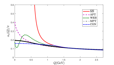
Figure 1: Typical $\alpha_{s}$-running behavior in low-energy scales for four typical low-energy models, APT, WEB, MPT, and CON, respectively. The $\alpha_{s}$-running behavior derived from RGE under $\overline{\rm MS}$-scheme is given as a comparison.

To do the numerical analysis, we take the nucleon axial charge ratio $g_{A}=1.2724\pm 0.0023$ PDG:2020 . The asymptotic QCD scale $\Lambda$ can be fixed by using the $\alpha_{s}$-value at the reference point such as $\alpha^{\overline{\rm MS}}_{s}(m_{\tau})=0.325\pm 0.016$ PDG:2020 , which gives $\Lambda_{\overline{\rm MS}}|_{n_{f}=3}=0.346^{+0.028}_{-0.029}$ GeV by using the four-loop RGE. Using the relation (28), we obtain $\Lambda_{\rm APT}|_{n_{f}=3}=0.244^{+0.033}_{-0.031}$ GeV. In Fig. 1, we present the typical running behaviors of $\alpha_{s}/\pi$ under four low-energy models, where the parameters are set to be $\xi=10$ for MPT and $m_{g}=700~{}\rm MeV$ for CON, respectively. The $\alpha_{s}$-running behavior derived from the RGE under $\overline{\rm MS}$-scheme is given as a comparison. Fig. 1 shows the importance of the using of low-energy models in the region of small energy-scale. Using the criteria suggested in Ref.Deur:2014qfa for the analytic matching of $\alpha_{s}$ in perturbative and nonperturbative regimes, we obtain the transition scales ($Q_{0}$) for various low-energy models, which are $\sim 1.77$ GeV, $\sim 1.78$ GeV, $\sim 1.78$ GeV, $\sim 1.19$ GeV for APT, WEB, MPT and CON models, respectively. As a subtle point, because the transition scales $Q_{0}$ for the cases of WEB and MPT are slightly bigger than $m_{\tau}$, and for self-consistency, we use the low-energy $\alpha^{\rm WEB/MPT}_{s}(m_{\tau})=0.325\pm 0.016$ to fix $\Lambda$, which is $0.206\pm{0.022}$ GeV or $0.294^{+0.033}_{-0.032}$ GeV, respecitvely.

For later convenience, in the following discussions, we simply use $\alpha_{s}^{\overline{\rm MS}}$ to stand for the case of using $\overline{\rm MS}$-scheme $\alpha_{s}$ in all $Q^{2}$-region, $\alpha_{s}^{\rm APT}$ to stand for the case of using APT model in low-energy region ($Q<Q_{0}$, as mentioned above, $Q_{0}$ is different for different low-energy model) and $\overline{\rm MS}$-scheme $\alpha_{s}$ in large $Q^{2}$-region, $\alpha_{s}^{\rm WEB}$ to stand for the case of using WEB model in low-energy model and $\overline{\rm MS}$-scheme $\alpha_{s}$ in large $Q^{2}$-region, $\alpha_{s}^{\rm MPT}$ to stand for the case of using MPT model in low-energy model and $\overline{\rm MS}$-scheme $\alpha_{s}$ in large $Q^{2}$-region, and $\alpha_{s}^{\rm CON}$ to stand for the case of using CON model in low-energy model and $\overline{\rm MS}$-scheme $\alpha_{s}$ in large $Q^{2}$-region.

III.1 Perturbative contributions to the leading-twist part of BSR up to $\rm{N^{4}LO}$ level

(a) Leading-twist contributions using $\alpha^{\rm APT}_{s}$.

(b) Leading-twist contributions using $\alpha^{\rm WEB}_{s}$.

(c) Leading-twist contributions using $\alpha^{\rm MPT}_{s}$.

(d) Leading-twist contributions using $\alpha^{\rm CON}_{s}$.

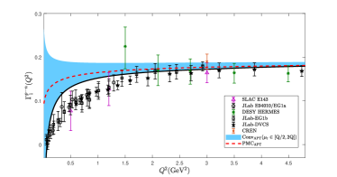
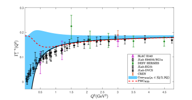
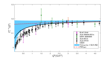
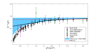
Figure 2: Perturbative leading-twist contributions to the spin structure function $\Gamma^{p-n}_{1}(Q^{2})$ up to $\rm{N^{3}LO}$ versus momentum Q, under four $\alpha_{s}$ models: (a) the APT model; (b) The WEB model; (c) the MPT model; and (d) the CON model. The solid line is for conventional scale setting approach with $\mu_{r}=Q$ and the shaded band shows its scale uncertainty by varying $\mu_{r}\in[Q/2,2Q]$. The dot-dashed line is the prediction $\Gamma^{p-n}_{1}(Q^{2})$ up to $\rm{N^{4}LO}$ for PMC scale-setting approach, which is free of renormalization scale dependence.

The perturbative contributions to the leading-twist part $E_{\rm ns}(Q^{2})$ has been known up to $\rm{N^{3}LO}$. Under conventional scale-setting approach, the pQCD series is scale dependent, and by setting $\mu_{r}=Q$, we obtain

$$E_{\rm ns}(Q^{2})|_{\rm Conv.} = a(Q)+3.58a^{2}(Q)+20.22a^{3}(Q)$$ (32)

$$+175.70a^{4}(Q).$$

On the other hand, the pQCD series becomes scale invariant by applying the PMC, and we obtain

$$E_{\rm ns}(Q^{2})|_{\rm PMC} = a(Q_{\star})+1.15a^{2}(Q_{\star})+0.14a^{3}(Q_{\star})$$ (33)

$$+0.76a^{4}(Q_{\star})$$

for any choice of renormalization scale, where $Q_{\star}$ is of perturbative nature, which can be determined up to NNLL accuracy

$$\ln\frac{{Q_{*}}^{2}}{Q^{2}} = -1.08-1.87a(Q)-24.06a^{2}(Q).$$ (34)

One may observe that the perturbative coefficients in PMC series (33) are much smaller than those of conventional series (32), especially for those of high-orders, which are due to the elimination of divergent renormalon terms as $n!\beta^{n}_{0}a_{s}^{n}$. This indicates that a much more convergent perturbative series can be achieved by applying the PMC. At the same time, the PMC scale $Q_{\star}$ also shows a fast convergent at high $Q$-range, e.g. the relative absolute values of the LL, the NLL and the NNLL terms are 1: 0.064 : 0.030 for $Q=100$ GeV. Thus the residual scale dependence due to unknown even higher-order terms can be greatly suppressed.

Using the convergent PMC perturbative series, one can obtain a reliable prediction of unknown $\mathcal{O}(a^{5})$-term by using the PAA, e.g. by using Eq.(22), we obtain

$$E_{\rm ns}(Q^{2})|^{\rm N^{4}LO}_{\rm PAA}=2.92a^{5}(Q_{\star}).$$ (35)

We present the predicted leading-twist part of the spin structure function $\Gamma^{p-n}_{1}(Q^{2})$ under four low-energy models in Fig. 2, where the results under conventional and PMC scale-setting approaches are presented. The experimental data are from SLAC Abe:1994cp ; Abe:1995mt ; Abe:1995dc ; Abe:1995rn ; Abe:1998wq , DESY Ackerstaff:1997ws ; Ackerstaff:1998ja ; Airapetian:1998wi ; Airapetian:2002rw ; Airapetian:2006vy , CREN Alexakhin:2006oza ; Alekseev:2010hc ; Adolph:2015saz and JLab Deur:2004ti ; Deur:2008ej ; Deur:2014vea . The PMC predictions are independent to any choice of $\mu_{r}$, and the shaded band shows the conventional renormalization scale uncertainty by varying $\mu_{r}\in[Q/2,2Q]$. Under conventional scale-setting approach, the spin structure function $\Gamma^{p-n}_{1}(Q^{2})$ shows large scale dependence, especially in low-energy region. In low-energy region, the results by using the IR-fixed couplings are much more reliable. And since couplings behaves differently in low-energy region, the spin structure function $\Gamma^{p-n}_{1}(Q^{2})$ behaves quite differently for $Q\to 0$. When the energy scale is large enough, such as $Q>1.5-2.0$ GeV, the perturbative leading-twist terms could explain the experimental data well. Fig. 2 also shows that in low-scale region, the leading-twist terms alone cannot explain the data and one must take the high-twist terms into consideration. By comparing with the data, this fact inversely provides us a good platform to achieve reliable predictions on the magnitudes of high-twist contributions.

III.2 Analysis of high-twist contributions under various low-energy models

	$\alpha_{s}$ models		$f_{2}^{p-n}(1)$	$\mu_{6}$	$\chi^{2}/d.o.f$
		$\mu_{r}=Q/2$	$-0.176\pm{0.000}\pm{0.013}$	$0.004\pm{0.000}\pm{0.000}$	149
	$\rm{APT}|_{Conv}$	$\mu_{r}=Q$	$-0.088\pm{0.000}\pm{0.013}$	$0.002\pm{0.000}\pm{0.000}$	62
		$\mu_{r}=2Q$	$-0.107\pm{0.000}\pm{0.013}$	$0.003\pm{0.000}\pm{0.000}$	117
	$\rm{APT|_{PMC}}$	$\mu_{r}\in[Q/2,2Q]$	$-0.120\pm{0.000}\pm{0.013}$	$0.003\pm{0.000}\pm{0.000}$	62
		$\mu_{r}=Q/2$	$-0.193\pm{0.000}\pm{0.013}$	$0.005\pm{0.000}\pm{0.000}$	193
	$\rm{WEB}|_{Conv}$	$\mu_{r}=Q$	$-0.047\pm{0.000}\pm{0.013}$	$0.001\pm{0.000}\pm{0.000}$	168
		$\mu_{r}=2Q$	$-0.105\pm{0.000}\pm{0.013}$	$0.004\pm{0.000}\pm{0.000}$	160
	$\rm{WEB|_{PMC}}$	$\mu_{r}\in[Q/2,2Q]$	$-0.081\pm{0.000}\pm{0.013}$	$0.001\pm{0.000}\pm{0.000}$	45
		$\mu_{r}=Q/2$	$-0.173\pm{0.000}\pm{0.013}$	$0.004\pm{0.000}\pm{0.000}$	151
	$\rm{MPT}|_{Conv}$	$\mu_{r}=Q$	$-0.080\pm{0.000}\pm{0.013}$	$0.002\pm{0.000}\pm{0.000}$	56
		$\mu_{r}=2Q$	$-0.105\pm{0.000}\pm{0.013}$	$0.003\pm{0.000}\pm{0.000}$	126
	$\rm{MPT|_{PMC}}$	$\mu_{r}\in[Q/2,2Q]$	$-0.128\pm{0.000}\pm{0.013}$	$0.003\pm{0.000}\pm{0.000}$	50
		$\mu_{r}=Q/2$	$-0.175\pm{0.000}\pm{0.013}$	$0.003\pm{0.000}\pm{0.000}$	125
	$\rm{CON}|_{Conv}$	$\mu_{r}=Q$	$-0.070\pm{0.000}\pm{0.013}$	$0.001\pm{0.000}\pm{0.000}$	60
		$\mu_{r}=2Q$	$-0.102\pm{0.000}\pm{0.013}$	$0.002\pm{0.000}\pm{0.000}$	138
	$\rm{CON|_{PMC}}$	$\mu_{r}\in[Q/2,2Q]$	$-0.139\pm{0.001}\pm{0.013}$	$0.002\pm{0.000}\pm{0.000}$	49

Table 1: The fitted parameters $f^{p-n}_{2}(Q^{2}=1~{}\rm GeV^{2})$ and $\mu_{6}$ and their corresponding quality of fit $\chi^{2}/d.o.f$ under four $\alpha_{s}$ models before and after applying the PMC, where the first and the second errors are caused by the statistical and systematic errors of the data Deur:2008ej ; Deur:2014vea . The twist-6 coefficient $\mu_{6}$ is almost independent to the choices of statistical and systematic errors.

Following the discussions of Sec.II.B, we need to fit two parameters, $f^{p-n}_{2}(1~{}\rm GeV^{2})$ and $\mu_{6}$, so as to determine the high-twist contributions. We adopt the most recent data listed in Refs.Deur:2008ej ; Deur:2014vea to do the fitting, whose momentum transfer lies in the range of ${0.054}~{}{\rm GeV^{2}}\leq Q^{2}\leq 4.739~{}{\rm GeV^{2}}$. We adopt the APT, WEB, MPT, and the CON couplings in doing the fitting. The quality of fit is measured by the parameter of $\chi^{2}/d.o.f$, e.g.

$$\chi^{2}/{d.o.f}={1\over{N-d}}\sum\limits^{N}_{j=1}\frac{(\Gamma^{p-n}_{1,{\rm the.}}(Q^{2}_{j})-\Gamma^{p-n}_{1,{\rm exp.}}(Q^{2}_{j}))^{2}}{\sigma^{2}_{j,{\rm stat.}}},$$ (36)

where the symbol “$d.o.f$” (short notation of the degree of freedom) is equal to $N-d$ with $N=31$ being the number of data points and $d=2$ being the number of fitted parameters, “the.” stands for theoretical prediction, “exp.” stands for measured value, and “$\sigma_{j,{\rm stat.}}$” is the statistical error at each point $Q_{j}$. Comparing theoretical prediction $\Gamma^{p-n}_{1,{\rm the.}}(Q^{2}_{j})$ with the measured value $\Gamma^{p-n}_{1,{\rm exp.}}(Q^{2}_{j})$ at all the data points $Q_{j\in[1,N]}$, we can derive the preferable $f^{p-n}_{2}$ and $\mu_{6}$ by requiring them to achieve the minimum value of $\chi^{2}/d.o.f$. To do the fitting, we also take into account the systematic error $\sigma_{j,{\rm sys.}}$ at each point $Q_{j}$, which has sizable contributions to the fitted values of $f^{p-n}_{2}$ and $\mu_{6}$. For convenience, we put the detailed calculation technology in Appendix B.

Our results for the two parameters $f^{p-n}_{2}(1~{}\rm GeV^{2})$ and $\mu_{6}$ are presented in Table. 1. The right-most column shows the smallest $\chi^{2}/d.o.f$ for the predictions before and after applying the PMC under four $\alpha_{s}$ models. The magnitudes of those two parameters are small, which agree with the usual consideration that at large $Q^{2}$-region, the high-twist terms are power suppressed and are negligible. However in low $Q^{2}$-region, they will have sizable contributions; especially $f^{p-n}_{2}(1~{}\rm GeV^{2})$ is important for a reliable theoretical prediction on $\Gamma^{p-n}_{1,{\rm the.}}(Q^{2})$ in low $Q^{2}$-region. Table. 1 shows that the fitted parameters under conventional scale-setting approach have strong scale dependence, whose quality of fit $\chi^{2}/d.o.f$ varies from tens to hundreds, and the optimal fit are achieved for the case of $\mu_{r}\sim Q$. This, together with a better pQCD convergence due to the elimination of divergent log-terms $\ln\mu_{r}^{2}/Q^{2}$, in some sense explain why $\mu_{r}=Q$ is usually taken as the preferable renormalization scale for conventional scale-setting approach. On the other hand, the fitted parameters for the PMC scale-setting approach is independent for any choice of renormalization scale, thus a more reliable and accurate prediction is achieved.

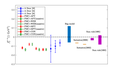
Figure 3: The twist-4 coefficient $f_{2}^{p-n}(1{\rm~{}GeV^{2}})$ obtained from the PMC predictions under four $\alpha_{s}$ low-energy models, in which the predictions using JLab data Deur:2004ti ; Deur:2008ej ; Deur:2014vea , the QCD sum rule predictions Stein:1995si ; Balitsky:1989jb , and the predictions using the model of the instanton-based QCD vacuum Lee:2001ug ; Sidorov:2006vu and the Bag model prediction Ji:1993sv are also presented.

At present, the twist-4 coefficient $f^{p-n}_{2}(1~{}\rm GeV^{2})$ has been calculated under various approaches, such as Refs. Stein:1995si ; Balitsky:1989jb ; Lee:2001ug ; Sidorov:2006vu ; Ji:1993sv ; Deur:2004ti ; Deur:2008ej ; Deur:2014vea ; Balla:1997hf . We present a comparison of various predictions in Fig. 3. The results of Refs.Deur:2004ti ; Deur:2008ej ; Deur:2014vea are fitted by using conventional pQCD series for the leading-twist part with fixing $\mu_{r}=Q$ and the JLab data within different ranges, $0.8~{}{\rm GeV^{2}}<Q^{2}_{j}<10~{}{\rm GeV^{2}}$ Deur:2004ti , $0.66~{}{\rm GeV^{2}}<Q^{2}_{j}<10~{}{\rm GeV^{2}}$ Deur:2008ej and $0.84~{}{\rm GeV^{2}}<Q^{2}_{j}<10~{}{\rm GeV^{2}}$ Deur:2014vea . By using $f^{p-n}_{2}$, we can evaluate the color polarizability, $\chi_{E}^{p-n}={2\over 3}(2d^{p-n}_{2}+f^{p-n}_{2})$ and $\chi_{B}^{p-n}={1\over 3}(4d^{p-n}_{2}-f^{p-n}_{2})$, which describes the response of the color magnetic and electric fields to the spin of the nucleon Ji:1995qe ; Stein:1995si . Using the PMC predictions for the hard-part of the leading-twist contributions, we obtain

$$\chi_{B}^{p-n}|_{\rm{APT}} = 0.051\pm 0.009,$$ (37)

$$\chi_{B}^{p-n}|_{\rm{WEB}} = 0.038\pm 0.009,$$ (38)

$$\chi_{B}^{p-n}|_{\rm{MPT}} = 0.053\pm 0.009,$$ (39)

$$\chi_{B}^{p-n}|_{\rm{CON}} = 0.057\pm 0.009,$$ (40)

$$\chi_{E}^{p-n}|_{\rm{APT}} = -0.069\pm 0.013,$$ (41)

$$\chi_{E}^{p-n}|_{\rm{WEB}} = -0.043\pm 0.013,$$ (42)

$$\chi_{E}^{p-n}|_{\rm{MPT}} = -0.075\pm 0.013,$$ (43)

$$\chi_{E}^{p-n}|_{\rm{CON}} = -0.082\pm 0.013,$$ (44)

where the errors are squared average of those from $\Delta d^{p-n}_{2}=\pm 0.0036$ and $\Delta f^{p-n}_{2}$ for the four low-energy $\alpha_{s}$ models (e.g. Table. 1).

(a) APT model

(b) WEB model

(c) MPT model

(d) CON model

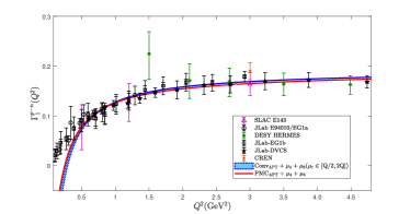
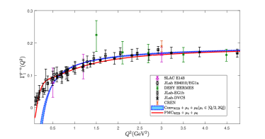
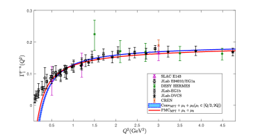
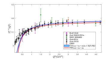
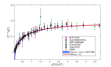
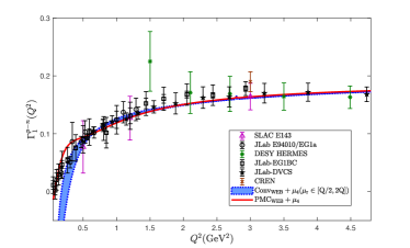
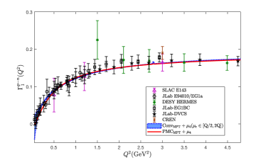
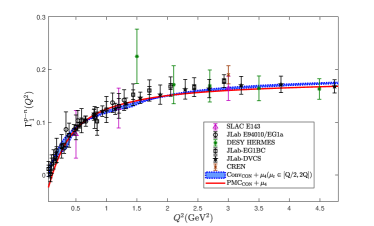
Figure 4: The spin structure function $\Gamma^{p-n}_{1}(Q^{2})$ with both leading-twist and high-twist contributions under four $\alpha_{s}$ models: (a) the APT model; (b) the WEB model; (c) the MPT model; and (d) the CON model. The leading-twist perturbative contributions have been calculated up to ${\rm N^{3}LO}$ level and ${\rm N^{4}LO}$ level before and after applying the PMC scale-setting approach, respectively. The shaded band shows the prediction under conventional scale-setting approach by varying $\mu_{r}\in[Q/2,2Q]$. The solid line is the scale-invariant PMC prediction.

We present the prediction of $\Gamma^{p-n}_{1}(Q^{2})$ with both leading-twist and high-twist contributions in Fig. 4. Comparing with Fig. 2, Fig. 4 shows that a more reasonable prediction can be achieved by including high-twist contributions. Under conventional scale-setting approach, the large scale dependence for the leading-twist prediction of $\Gamma^{p-n}_{1,{\rm Conv.}}(Q^{2})$ can be greatly suppressed by including high-twist terms due to the cancellation of scale dependence among different twist-terms. Under PMC scale-setting approach, the scale-invariant $\Gamma^{p-n}_{1,{\rm PMC}}(Q^{2})$ under APT, MPT and CON $\alpha_{s}$ models are close in shape, which as shown by Table. 1 also have close quality of fit $\chi^{2}/d.o.f$; while the PMC prediction under WEB model is slightly different from those of other $\alpha_{s}$ models.

As a final remark, to improve the quality of fit, as suggested by Ref.Ayala:2018ulm , we use the JLab data points with $Q^{2}>0.268~{}{\rm GeV^{2}}$ to do fit. By using the scale-invariant PMC pQCD series, the quality of fit $\chi^{2}/d.o.f$ improves to be $\sim 34$ for APT model, $\sim 52$ for WEB model, $\sim 34$ for MPT model and $\sim 38$ for CON model, respectively, which correspond to the $p$-value around $95\%-99\%$ PDG:2020 .

III.3 An analysis of high-twist contributions with massive high-twist expression

As shown by Fig. 4, the predictions drops down quickly in very small $Q^{2}$-region, and the quality of fit is greatly affected by the data within this $Q^{2}$-region, indicating the twist-expansion could be failed in very small $Q^{2}$-region. It has been suggested that by using the “massive” high-twist expansion to do the data fitting, cf. Ayala:2018ulm ; Ayala:2020scz ; Teryaev:2013qba ; Khandramai:2016kbh ; Gabdrakhmanov:2017dvg ; Aguilar:2014tka , one may obtain a better explanation of the data in very low $Q^{2}$ region. As an attempt, we take the following “massive” high-twist expansion to do the fit Ayala:2018ulm

$$\Gamma^{p-n}_{1}(Q^{2})=\frac{g_{A}}{6}\left[1-E_{\rm ns}(Q^{2})\right]+\frac{\mu^{p-n}_{4}}{Q^{2}+m^{2}}+\cdots,$$ (45)

where the parameter $m$ represents a dynamical effective gluon mass, whose square satisfies

$$m^{2}=\frac{m^{2}(1~{}\rm GeV^{2})(1+1/\mathcal{M}^{2})^{1+\rm p}}{(1+Q^{2}/\mathcal{M}^{2})^{1+{\rm p}}}.$$ (46)

Here we have set the initial scale of the squared mass as $1$ GeV, and we shall take the parameters $\mathcal{M}^{2}=0.5~{}{\rm GeV}^{2}$ and $\rm p=0.1$ to do the calculation, which are within the suggested range of Ref.Aguilar:2014tka . At present, to fit the magnitude of the “massive” high-twist terms, the parameters $f^{p-n}_{2}(1~{}\rm GeV^{2})$ and $m^{2}(1~{}\rm GeV^{2})$ are used to fit with the data Deur:2008ej ; Deur:2014vea . When doing the fitting with the experiments data within the range of $0.054\rm GeV^{2}\leq Q^{2}\leq 4.739\rm GeV^{2}$, we adopt four $\alpha_{s}$ models. The results for the two parameters $f^{p-n}_{2}(1~{}\rm GeV^{2})$, $m^{2}(1~{}\rm GeV^{2})$ and their corresponding quality of fit $\chi^{2}/d.o.f$ are presented in Table. 2. Those two parameters are obtained by considering the systematic error $\sigma_{j,sys}$ at each data point $Q^{2}_{j}$ into the fitting; We put the details of fitting in the end of Appendix B. Comparing the smallest $\chi^{2}/d.o.f$ listed in Table. 1 and Table. 2, one may observes that the “massive” BSR shows a better behavior with smaller quality of fit $\chi^{2}/d.o.f$. The conventional predictions for twist-4 $f^{p-n}_{2}(1~{}\rm GeV^{2})$ apparently depends on the choice of $\mu_{r}$. The quality of fit $\chi^{2}/d.o.f$ for conventional predictions with $\alpha_{s}$ under WEB model varies from tens to hundreds, while similar $\chi^{2}/d.o.f$ for conventional predictions with $\alpha_{s}$ under APT, MPT and CON models are along with different fit parameters $f^{p-n}_{2}(1~{}\rm GeV^{2})$ and $m^{2}(1~{}\rm GeV^{2})$, respectively. If using the PMC scale-independent series and the “massive” high-twist term, we can obtain the corresponding color polarizability $\chi^{p-n}_{E}$ and $\chi^{p-n}_{B}$:

$$\chi_{B}^{p-n}|_{\rm{APT}} = 0.057\pm 0.009,$$ (47)

$$\chi_{B}^{p-n}|_{\rm{WEB}} = 0.038\pm 0.009,$$ (48)

$$\chi_{B}^{p-n}|_{\rm{MPT}} = 0.057\pm 0.009,$$ (49)

$$\chi_{B}^{p-n}|_{\rm{CON}} = 0.060\pm 0.009,$$ (50)

$$\chi_{E}^{p-n}|_{\rm{APT}} = -0.083\pm 0.014,$$ (51)

$$\chi_{E}^{p-n}|_{\rm{WEB}} = -0.043\pm 0.014,$$ (52)

$$\chi_{E}^{p-n}|_{\rm{MPT}} = -0.082\pm 0.014,$$ (53)

$$\chi_{E}^{p-n}|_{\rm{CON}} = -0.087\pm 0.014,$$ (54)

where the errors are squared average of those from $\Delta d^{p-n}_{2}=\pm 0.0036$ and $\Delta f^{p-n}_{2}$ for the four low-energy $\alpha_{s}$ models (e.g. Table. 2).

	$\alpha_{s}$ models		$f_{2}^{p-n}(1)$	${m}^{2}(1)$	$\chi^{2}/d.o.f$
		$\mu_{r}=Q/2$	$-0.217\pm{0.004}\pm{0.013}$	$0.203\pm{0.016}\pm{0.102}$	48
	$\rm{APT}|_{Conv}$	$\mu_{r}=Q$	$-0.113\pm{0.004}\pm{0.013}$	$0.285\pm{0.041}\pm{0.249}$	42
		$\mu_{r}=2Q$	$-0.166\pm{0.005}\pm{0.013}$	$0.505\pm{0.045}\pm{0.205}$	43
	$\rm{APT|_{PMC}}$	$\mu_{r}\in[Q/2,2Q]$	$-0.140\pm{0.004}\pm{0.013}$	$0.162\pm{0.021}\pm{0.011}$	28
		$\mu_{r}=Q/2$	$-0.235\pm{0.004}\pm{0.013}$	$0.184\pm{0.013}\pm{0.006}$	37
	$\rm{WEB}|_{Conv}$	$\mu_{r}=Q$	$-0.138\pm{0.009}\pm{0.013}$	$2.233\pm{0.373}\pm{0.044}$	80
		$\mu_{r}=2Q$	$-0.183\pm{0.006}\pm{0.013}$	$0.717\pm{0.056}\pm{0.026}$	145
	$\rm{WEB|_{PMC}}$	$\mu_{r}\in[Q/2,2Q]$	$-0.081\pm{0.003}\pm{0.013}$	$0.038\pm{0.010}\pm{0.011}$	45
		$\mu_{r}=Q/2$	$-0.220\pm{0.004}\pm{0.013}$	$0.220\pm{0.016}\pm{0.046}$	44
	$\rm{MPT}|_{Conv}$	$\mu_{r}=Q$	$-0.099\pm{0.004}\pm{0.013}$	$0.229\pm{0.043}\pm{0.044}$	38
		$\mu_{r}=2Q$	$-0.168\pm{0.005}\pm{0.013}$	$0.538\pm{0.047}\pm{0.058}$	40
	$\rm{MPT|_{PMC}}$	$\mu_{r}\in[Q/2,2Q]$	$-0.139\pm{0.004}\pm{0.013}$	$0.096\pm{0.015}\pm{0.009}$	29
		$\mu_{r}=Q/2$	$-0.215\pm{0.004}\pm{0.013}$	$0.191\pm{0.016}\pm{0.007}$	39
	$\rm{CON}|_{Conv}$	$\mu_{r}=Q$	$-0.071\pm{0.003}\pm{0.013}$	$0.045\pm{0.020}\pm{0.016}$	60
		$\mu_{r}=2Q$	$-0.174\pm{0.005}\pm{0.013}$	$0.605\pm{0.052}\pm{0.019}$	37
	$\rm{CON|_{PMC}}$	$\mu_{r}\in[Q/2,2Q]$	$-0.147\pm{0.004}\pm{0.013}$	$0.075\pm{0.011}\pm{0.008}$	36

Table 2: The fitted parameters $f^{p-n}_{2}(Q^{2}=1~{}\rm GeV^{2})$ and ${m}^{2}(Q^{2}=1~{}\rm GeV^{2})$ and their corresponding quality of fit $\chi^{2}/d.o.f$ under four $\alpha_{s}$ models before and after applying the PMC, where the first and the second errors are caused by the statistical and systematic errors of the experiments data.

To compare with Fig. 4, Fig. 5 shows that by using the “massive” high-twist term with the fitted parameters $f^{p-n}_{2}(1~{}\rm GeV^{2})$ and $m^{2}(1~{}\rm GeV^{2})$, a better prediction in agreement with the experiments data for $Q^{2}$ below 0.5 $\rm GeV^{2}$ can be achieved, which results as a smaller $\chi^{2}/d.o.f$ in Table. 2. Different from the PMC predictions, the scale-dependence for conventional predictions is enhanced in small $Q^{2}$ region. Then, without renormalization scale dependence, the PMC predictions for the twist-4 contribution are more reliable; more explicitly, we observe that the quality of fit $\chi^{2}/d.o.f$ can be improved as $\sim 28$ for APT model, $\sim 45$ for WEB model, $\sim 29$ for MPT model and $\sim 36$ for CON model, respectively, all of which correspond to a $p$-value $\geq 99\%$.

(a) APT model

(b) WEB model

(c) MPT model

(d) CON model

Figure 5: The spin structure function $\Gamma^{p-n}_{1}(Q^{2})$ with both leading-twist and the “massive” high-twist contributions under four $\alpha_{s}$ models: (a) the APT model; (b) the WEB model; (c) the MPT model; and (d) the CON model. The leading-twist perturbative contributions have been calculated up to ${\rm N^{3}LO}$ level and ${\rm N^{4}LO}$ level before and after applying the PMC scale-setting approach, respectively. The shaded band shows the prediction under conventional scale-setting approach by varying $\mu_{r}\in[Q/2,2Q]$. The solid line is the scale-invariant PMC prediction.

IV Summary

In the paper, we have applied the PMC single-scale approach to deal with the perturbative series of the leading-twist part of $\Gamma^{p-n}_{1}(Q^{2})$ up to ${\rm N^{3}LO}$ level. The pQCD series for both $\Gamma^{p-n}_{1}(Q^{2})$ and the PMC scale $Q_{*}$ are convergent in large $Q^{2}$-region. We have also provided a prediction on the uncalculated ${\rm N^{4}LO}$ by using the more convergent and scheme-and-scale invariant PMC conformal series. Thus a more accurate pQCD prediction on $\Gamma^{p-n}_{1}(Q^{2})$ can be achieved by applying the PMC.

Basing on the PMC predictions on the perturbative part, we then provide a novel determination of the high-twist contributions by using the JLab data, whose momentum transfer lies in the range of ${0.054}~{}{\rm GeV^{2}}\leq Q^{2}\leq 4.739~{}{\rm GeV^{2}}$. In large $Q^{2}$-region, the high-twist contributions to $\Gamma^{p-n}_{1}(Q^{2})$ are power suppressed and negligible, which are however sizable in low and intermediate $Q^{2}$-region; Fig. 2 shows that in low $Q^{2}$-region, the leading-twist terms alone cannot explain the JLab data. The high-twist term is necessary and it can fix this problem with two fit parameters as Fig. 5 shows. Taking the high-twist contributions up to twist-6 accuracy, we have fixed the twist-4 coefficient $f_{2}^{p-n}$ and the twist-6 coefficient $\mu_{6}$ by using four typical $\alpha_{s}$-models, which give $f_{2}^{p-n}|_{\rm APT}=-0.120\pm 0.013$ and $\mu_{6}|_{\rm APT}=0.003\pm{0.000}$, $f_{2}^{p-n}|_{\rm WEB}=-0.081\pm 0.013$ and $\mu_{6}|_{\rm WEB}=0.001\pm{0.000}$, $f_{2}^{p-n}|_{\rm MPT}=-0.128\pm 0.013$ and $\mu_{6}|_{\rm MPT}=0.003\pm{0.000}$, $f_{2}^{p-n}|_{\rm CON}=-0.139\pm 0.013$ and $\mu_{6}|_{\rm CON}=0.002\pm 0.000$, respectively. Here the errors are squared averages of those from the statistical and systematic errors of the measured data. As an attempt, by taking the “massive” high-twist expansion such as Eq.(45) to do the fit, we have shown that a better explanation of the data in very low $Q^{2}$ range can be achieved.

Acknowledgments: This work was supported in part by the Natural Science Foundation of China under Grant No.11625520 and No.12047564, by graduate research and innovation foundation of Chongqing, China (Grant No.CYB21045), by the Fundamental Research Funds for the Central Universities under Grant No.2020CQJQY-Z003, and by the Chongqing Graduate Research and Innovation Foundation under Grant No.ydstd1912.

Appendix A the reduced perturbative coefficients ${\hat{r}}_{i,j}$

In this appendix, we give the required reduced coefficients $\hat{r}_{i,j}$ for the perturbative series of the leading-twist part of $\Gamma^{p-n}_{1}(Q^{2},\mu_{r})$ up to four-loop level, i.e.,

$${\hat{r}}_{1,0} = \frac{3}{4}{\gamma^{\rm ns}_{1}},$$

$${\hat{r}}_{2,0} = \frac{3}{4}{\gamma^{\rm ns}_{2}}-\frac{9}{16}\big{(}{\gamma^{\rm ns}_{1}}\big{)}^{2},$$

$${\hat{r}}_{2,1} = {3\over 4}{\Pi^{\rm ns}_{1}}+{K^{\rm ns}_{1}},$$

$${\hat{r}}_{3,0} = \frac{3}{4}{\gamma^{\rm ns}_{3}}-\frac{9}{8}{\gamma^{\rm ns}_{2}}{\gamma^{\rm ns}_{1}}+\frac{27}{64}\big{(}{\gamma^{\rm ns}_{1}}\big{)}^{3},$$

$${\hat{r}}_{3,1} = {3\over 4}{\Pi^{\rm ns}_{2}}+{1\over 2}{K^{\rm ns}_{2}}-\frac{\gamma^{\rm ns}_{1}}{4}\left(\frac{3}{2}{K^{\rm ns}_{1}}+{9\over 4}{\Pi^{\rm ns}_{1}}\right),$$

$${\hat{r}}_{3,2} = 0,$$

$${\hat{r}}_{4,0} = \frac{3}{4}{\gamma^{\rm ns}_{4}}-\frac{9}{8}{\gamma^{\rm ns}_{3}}{\gamma^{\rm ns}_{1}}-\frac{9}{16}\big{(}{\gamma^{\rm ns}_{2}}\big{)}^{2}$$

$$+\frac{81}{64}{\gamma^{\rm ns}_{2}}\big{(}{\gamma^{\rm ns}_{1}}\big{)}^{2}-\frac{81}{256}\big{(}{\gamma^{\rm ns}_{1}}\big{)}^{4},$$

$${\hat{r}}_{4,1} = {3\over 4}{\Pi^{\rm ns}_{3}}+{1\over 3}{K^{\rm ns}_{3}}-{1\over 4}{\gamma^{\rm ns}_{1}}\left({K^{\rm ns}_{2}}+3{\Pi^{\rm ns}_{2}}\right)$$

$$-\frac{\gamma^{\rm ns}_{2}}{4}\left({K^{\rm ns}_{1}}+{3\over 2}{\Pi^{\rm ns}_{1}}\right)+\frac{\big{(}{\gamma^{\rm ns}_{1}}\big{)}^{2}}{16}\left(3{K^{\rm ns}_{1}}+\frac{27}{4}{\Pi^{\rm ns}_{1}}\right),$$

$${\hat{r}}_{4,2} = -\frac{3}{16}\big{(}{\Pi^{\rm ns}_{1}}\big{)}^{2}-{1\over 4}{K^{\rm ns}_{1}}{\Pi^{\rm ns}_{1}},$$

$${\hat{r}}_{4,3} = 0,$$

where $\gamma^{\rm ns}_{i}$, $\Pi^{\rm ns}_{i}$ and $K^{\rm ns}_{i}$ can be found in Refs.Baikov:2010je ; Baikov:2012zm .

Appendix B Derivation of the parameters $f^{p-n}_{2}(1~{}{\rm GeV^{2}})$ and $\mu_{6}$

According to Ref.Ayala:2018ulm , it is straightforward to deduce the squares of the standard deviation of $f^{p-n}_{2}(1{~{}\rm GeV^{2}})$ and $\mu_{6}$, based on the minimization of $\chi^{2}/d.o.f$. Comparing the experimental data $\Gamma^{p-n}_{1,{\rm exp}}(Q^{2})$ and theoretical prediction $\Gamma^{p-n}_{1,{\rm the}}(Q^{2})$, we describe this difference at a specific point $Q^{2}_{j}$ by using the following symbol:

$$y_{j}\equiv\Gamma^{p-n}_{1,{\rm exp}}(Q^{2}_{j})-\Gamma^{p-n}_{1,{\rm the}}(Q^{2}_{j}).$$ (55)

The quality parameter $\chi^{2}$ is rewritten as

$$\chi^{2}(\mu_{4},\mu_{6})=\sum_{j}w_{j}(y_{j}-\mu_{4}z_{j}-\mu_{6}z^{2}_{j})^{2}.$$ (56)

where $z_{j}\equiv 1/Q^{2}_{j}$ and $w_{j}\equiv 1/\sigma^{2}_{j,{\rm stat}}$ from the squared statistical uncertainties of experimental values. The values $\hat{\mu}_{4}$ and $\hat{\mu}_{6}$ can be obtained by the condition: the simultaneous minimization of $\chi^{2}(\mu_{4},\mu_{6})$. Here the reduced values of $\hat{\mu}_{4}$ and $\hat{\mu}_{6}$ are defined as

$$\hat{\mu}_{4}=\frac{-\overline{yz^{2}}~{}\overline{z^{3}}+\overline{yz}~{}\overline{z^{4}}}{\overline{z^{2}}~{}\overline{z^{4}}-\overline{z^{3}}~{}\overline{z^{3}}},\hat{\mu}_{6}=\frac{\overline{yz^{2}}~{}\overline{z^{2}}-\overline{yz}~{}\overline{z^{3}}}{\overline{z^{2}}~{}\overline{z^{4}}-\overline{z^{3}}~{}\overline{z^{3}}}$$ (57)

with the unnormalized “average”

$$\overline{A}\equiv\sum_{j}w_{j}A(z_{j}).$$ (58)

Simplifying $f^{p-n}_{2}$ and $\mu_{6}$ as constants, there are the following approximations: the statistical uncertainties at different points are considered as uncorrelated; the systematical uncertainties at different point are considered as uncorrelated between different experiments but correlated under the same experiment.

After using Taylor expansion of $\chi^{2}(\mu_{4},\mu_{6})$ around the point $(\hat{\mu}_{4},\hat{\mu}_{6})$ up to the terms quadratic in the deviations, the approximate relations are Ayala:2018ulm

$$\chi^{2}(\hat{\mu}_{4}+\sigma(\hat{\mu}^{\rm stat}_{4}),\hat{\mu}_{6})=\chi^{2}_{\rm min}+\frac{\overline{z^{2}}~{}\overline{z^{4}}}{\overline{z^{2}}~{}\overline{z^{4}}-\overline{z^{3}}~{}\overline{z^{3}}},$$ (59)

$$\chi^{2}(\hat{\mu}_{4},\hat{\mu}_{6}+\sigma(\hat{\mu}^{\rm stat}_{6}))=\chi^{2}_{\rm min}+\frac{\overline{z^{2}}~{}\overline{z^{4}}}{\overline{z^{2}}~{}\overline{z^{4}}-\overline{z^{3}}~{}\overline{z^{3}}}.$$ (60)

Thus, the statistical uncertainties of fits parameters $\mu_{4}$ and $\mu_{6}$ can be obtained from Eqs.(59,60), and $\sigma(\hat{f}^{stat}_{2})=\frac{9}{4M^{2}}\sigma(\hat{\mu}^{stat}_{4})$ from Eq.(23).

Moreover, the calculation of systematical uncertainties of the parameters $\mu_{4}$ and $\mu_{6}$ at different point should consider the weighted mean values of different experiments. From this, we firstly express the quantities $\overline{yz^{2}}$ and $\overline{yz}$ in form of $\hat{\mu}_{4}$ and $\hat{\mu}_{6}$

$$\overline{yz}=\hat{\mu}_{4}\overline{z^{2}}+\hat{\mu}_{6}\overline{z^{3}},\overline{yz^{2}}=\hat{\mu}_{4}\overline{z^{3}}+\hat{\mu}_{6}\overline{z^{4}},$$ (61)

Considering the two different experimental group from Refs.Deur:2008ej ; Deur:2014vea , the $\hat{\mu}_{4}$ and $\hat{\mu}_{6}$ redefined by

$$\hat{\mu}_{4} = \tilde{\mu}^{(1)}_{4}+\tilde{\mu}^{(2)}_{4},$$ (62)

$$\hat{\mu}_{6} = \tilde{\mu}^{(1)}_{6}+\tilde{\mu}^{(2)}_{6},$$ (63)

and

$$\tilde{\mu}^{(i)}_{4} = \tilde{\alpha}_{i}\hat{\mu}^{(i)}_{4}-\tilde{k}_{i}\hat{\mu}^{(i)}_{6},$$ (64)

$$\tilde{\mu}^{(i)}_{6} = \tilde{\beta}_{i}\hat{\mu}^{(i)}_{6}+\tilde{h}_{i}\hat{\mu}^{(i)}_{4}.$$ (65)

where $i=1,2$ and weighted factors $\tilde{\alpha}_{i}$, $\tilde{\beta}_{i}$, $\tilde{k}_{i}$ and $\tilde{h}_{i}$ satisfying that

$$\tilde{\alpha}_{i} = \frac{1}{D^{\rm all}}(\sum^{2}_{j=1}D^{(ij)}),$$ (66)

$$\tilde{\beta}_{j} = \frac{1}{D^{\rm all}}(\sum^{2}_{i=1}D^{(ij)}),$$ (67)

$$\tilde{k}_{i} = \frac{1}{D^{\rm all}}\sum^{2}_{j=1:j\neq i}(-\overline{z^{3}}^{(i)}~{}\overline{z^{4}}^{(j)}+\overline{z^{3}}^{(j)}~{}\overline{z^{4}}^{(i)}),$$ (68)

$$\tilde{h}_{i} = \frac{1}{D^{\rm all}}\sum^{2}_{j=1:j\neq i}(-\overline{z^{2}}^{(i)}~{}\overline{z^{3}}^{(j)}+\overline{z^{2}}^{(j)}~{}\overline{z^{3}}^{(i)}),$$ (69)

$$D^{(ij)} = \overline{z^{2}}^{(i)}~{}\overline{z^{4}}^{(j)}-\overline{z^{3}}^{(i)}~{}\overline{z^{3}}^{(j)}~{}~{}(i,j=1,2),$$ (70)

$$D^{\rm all} = \sum^{2}_{j=1}\sum^{2}_{i=1}D^{(ij)}=\overline{z^{2}}~{}\overline{z^{4}}-\overline{z^{3}}\overline{z^{3}}.$$ (71)

The $D^{\rm all}$ is the unnormalized averages over two experiments. Then, we estimate the systematical uncertainty by averaging the deviations

$$\Delta\tilde{\mu}^{(i),{\rm sys}}_{N} \equiv\sigma(\tilde{\mu}^{(i),sys}_{N})$$ (72)

$$\approx\frac{1}{2}(|\tilde{\mu}^{(i)}_{N}({\rm UP})-\tilde{\mu}^{(i)}_{N}|+|\tilde{\mu}^{(i)}_{N}({\rm DO})-\tilde{\mu}^{(i)}_{N}|),$$

where $N=4,6$, symbols “UP” and “DO” refer to the values $\tilde{\mu}^{(i)}_{N}$ extracted from the experimental data plus or minus the uncertainty $\sigma_{j,{\rm sys}}$ at momentum $Q_{j}$, respectively. Finally, the systematical uncertainty $\Delta\hat{\mu}^{\rm sys}_{N}$ extracted from independent experiments are

$$\Delta\hat{\mu}^{\rm sys}_{4} \equiv \sigma(\tilde{\mu}^{\rm sys}_{4})=\bigg{[}\sum^{2}_{i=1}\sigma^{2}(\tilde{\mu}^{(i),sys}_{4})\bigg{]}^{1/2},$$ (73)

$$\Delta\hat{\mu}^{\rm sys}_{6} \equiv \sigma(\tilde{\mu}^{\rm sys}_{6})=\bigg{[}\sum^{2}_{i=1}\sigma^{2}(\tilde{\mu}^{(i),sys}_{6})\bigg{]}^{1/2},$$ (74)

and the corresponding uncertainties for the parameter $f^{p-n}_{2}(1~{}\rm GeV^{2})$ is

$$\Delta\hat{f}^{\rm sys}_{2}=\sigma(\hat{f}^{\rm sys}_{2})=\frac{9}{4M^{2}}\sigma(\hat{\mu}^{\rm sys}_{4}).$$ (75)

When using the “massive” high-twist expression (45), the squared standard deviation of $f^{p-n}_{2}(1{~{}\rm GeV^{2}})$ and $m^{2}(1{~{}\rm GeV^{2}})$ can be derived with the help of the minimization of $\chi^{2}/d.o.f$. If we expand the “massive” high-twist term in powers of $1/Q^{2}$, the twist-6 term can be expressed as

$$\mu_{6}(m^{2})=-m^{2}\mu_{4};~{}m^{2}=-\frac{\mu_{6}}{\mu_{4}}.$$ (76)

Using the approximate relations (59, 60), the statistical uncertainties of the extracted $f^{p-n}_{2}(1{~{}\rm GeV^{2}})$ and $m^{2}(1{~{}\rm GeV^{2}})$ are obtained from the following relations:

$$\chi^{2}(\hat{\mu}_{4}+\sigma(\hat{\mu}^{\rm stat}_{4}),\hat{m}^{2}) = \chi^{2}_{\rm min}+\frac{\overline{z^{2}}~{}\overline{z^{4}}}{\overline{z^{2}}~{}\overline{z^{4}}-\overline{z^{3}}~{}\overline{z^{3}}},$$ (77)

$$\chi^{2}(\hat{\mu}_{4},\hat{m}^{2}+\sigma(\hat{m}^{2}_{\rm stat})) = \chi^{2}_{\rm min}+\frac{\overline{z^{2}}~{}\overline{z^{4}}}{\overline{z^{2}}~{}\overline{z^{4}}-\overline{z^{3}}~{}\overline{z^{3}}}.$$ (78)

As for the systematic uncertainties of the “massive” case, i.e. the systematic uncertainty of $f^{p-n}_{2}(1{~{}\rm GeV^{2}})$ can obtained from Eq.(75) and the systematic uncertainty of $m^{2}(1{~{}\rm GeV^{2}})$ can be approximated by the following equations:

$$\sigma(\hat{m}^{2})_{\rm sys} \sim \bigg{(}\frac{\hat{\mu}_{6}}{\hat{\mu}^{2}_{4}}\bigg{)}^{2}\sigma^{2}(\hat{\mu}_{4})_{sys}+\frac{1}{\hat{\mu}^{2}_{4}}\sigma^{2}(\hat{\mu}_{6})_{sys}$$ (79)

$$- 2\bigg{(}\frac{\hat{\mu}_{6}}{\hat{\mu}^{3}_{4}}\bigg{)}<\delta\hat{\mu}_{4}\delta\hat{\mu}_{6}>_{sys},$$

$$<\delta\hat{\mu}_{4}\delta\hat{\mu}_{6}>_{sys} = \frac{1}{2}\sum^{2}_{i=1}\bigg{[}(\tilde{\mu}^{i}_{4}({\rm UP})-\tilde{\mu}^{i}_{4})(\tilde{\mu}^{i}_{6}({\rm UP})-\tilde{\mu}^{i}_{6})$$ (80)

$$+ (\tilde{\mu}^{i}_{4}({\rm DO})-\tilde{\mu}^{i}_{4})(\tilde{\mu}^{i}_{6}({\rm DO})-\tilde{\mu}^{i}_{6})\bigg{]}.$$

References

• (1) J. D. Bjorken, “Applications of the chiral U(6)×(6)𝑈66U(6)\times(6) algebra of current densities,” Phys. Rev.148, 1467 (1966).
• (2) J. D. Bjorken, “Inelastic Scattering of Polarized Leptons from Polarized Nucleons,” Phys. Rev. D 1, 1376 (1970).
• (3) P. L. Anthony et al. [E142 Collaboration], “Deep inelastic scattering of polarized electrons by polarized H3esuperscript𝐻3𝑒{}^{3}He and the study of the neutron spin structure,” Phys. Rev. D 54, 6620 (1996).
• (4) K. Abe et al. [E143 Collaboration], “Precision measurement of the proton spin structure function g1psuperscriptsubscript𝑔1𝑝g_{1}^{p},” Phys. Rev. Lett.  74, 346 (1995).
• (5) K. Abe et al. [E143 Collaboration], “Precision measurement of the deuteron spin structure function g1dsuperscriptsubscript𝑔1𝑑g_{1}^{d},” Phys. Rev. Lett.  75, 25 (1995).
• (6) K. Abe et al. [E143 Collaboration], “Measurements of the proton and deuteron spin structure function g2subscript𝑔2g_{2} and asymmetry A2subscript𝐴2A_{2},” Phys. Rev. Lett.  76, 587 (1996).
• (7) K. Abe et al. [E143 Collaboration], “Measurements of the Q2superscript𝑄2Q^{2} dependence of the proton and deuteron spin structure functions g1psuperscriptsubscript𝑔1𝑝g_{1}^{p} and g1dsuperscriptsubscript𝑔1𝑑g_{1}^{d},” Phys. Lett. B 364, 61 (1995)
• (8) K. Abe et al. [E154 Collaboration], “Measurement of the neutron spin structure function g2nsuperscriptsubscript𝑔2𝑛g_{2}^{n} and asymmetry A2nsuperscriptsubscript𝐴2𝑛A_{2}^{n},” Phys. Lett. B 404, 377 (1997).
• (9) K. Abe et al. [E154 Collaboration], “Next-to-leading order QCD analysis of polarized deep inelastic scattering data,” Phys. Lett. B 405, 180 (1997).
• (10) K. Abe et al. [E143 Collaboration], “Measurements of the proton and deuteron spin structure functions g1subscript𝑔1g_{1} and g2subscript𝑔2g_{2},” Phys. Rev. D 58, 112003 (1998)
• (11) P. L. Anthony et al. [E155 Collaboration], “Measurement of the proton and deuteron spin structure functions g2subscript𝑔2g_{2} and asymmetry A2subscript𝐴2A_{2},” Phys. Lett. B 458, 529 (1999).
• (12) P. L. Anthony et al. [E155 Collaboration], “Measurement of the deuteron spin structure function g1d(x)superscriptsubscript𝑔1𝑑𝑥g_{1}^{d}(x) for 1(GeV/c)2<Q2<40(GeV/c)21superscriptGeVc2superscriptQ240superscriptGeVc21\rm(GeV/c)^{2}<Q^{2}<40\rm(GeV/c)^{2},” Phys. Lett. B 463, 339 (1999).
• (13) P. L. Anthony et al. [E155 Collaboration], “Measurements of the Q2superscript𝑄2Q^{2} dependence of the proton and neutron spin structure functions g1psuperscriptsubscript𝑔1𝑝g_{1}^{p} and g1nsuperscriptsubscript𝑔1𝑛g_{1}^{n},” Phys. Lett. B 493, 19 (2000).
• (14) P. L. Anthony et al. [E155 Collaboration], “Precision measurement of the proton and deuteron spin structure functions g2subscript𝑔2g_{2} and asymmetries A2subscript𝐴2A_{2},” Phys. Lett. B 553, 18 (2003).
• (15) D. Adams et al. [SMC Collaboration], “Measurement of the spin dependent structure function g1(x)subscript𝑔1𝑥g_{1}(x) of the proton,” Phys. Lett. B 329, 399 (1994).
• (16) D. Adams et al. [SMC Collaboration], “Spin asymmetry in muon - proton deep inelastic scattering on a transversely polarized target,” Phys. Lett. B 336, 125 (1994).
• (17) D. Adams et al. [SMC Collaboration], “A New measurement of the spin dependent structure function g1(x)superscriptsubscript𝑔1𝑥g_{1}^{(x)} of the deuteron,” Phys. Lett. B 357, 248 (1995).
• (18) D. Adams et al. [SMC Collaboration], “The Spin dependent structure function g1(x)superscriptsubscript𝑔1𝑥g_{1}^{(x)} of the deuteron from polarized deep inelastic muon scattering,” Phys. Lett. B 396, 338 (1997).
• (19) D. Adams et al. [SMC Collaboration], “Spin structure of the proton from polarized inclusive deep inelastic muon - proton scattering,” Phys. Rev. D 56, 5330 (1997).
• (20) K. Ackerstaff et al. [HERMES Collaboration], “Measurement of the neutron spin structure function g1nsuperscriptsubscript𝑔1𝑛g_{1}^{n} with a polarized He-3 internal target,” Phys. Lett. B 404, 383 (1997).
• (21) K. Ackerstaff et al. [HERMES Collaboration], “Determination of the deep inelastic contribution to the generalized Gerasimov-Drell-Hearn integral for the proton and neutron,” Phys. Lett. B 444, 531 (1998).
• (22) A. Airapetian et al. [HERMES Collaboration], “Measurement of the proton spin structure function g1psuperscriptsubscript𝑔1𝑝g_{1}^{p} with a pure hydrogen target,” Phys. Lett. B 442, 484 (1998).
• (23) A. Airapetian et al. [HERMES Collaboration], “Evidence for quark hadron duality in the proton spin asymmetry A1subscript𝐴1A_{1},” Phys. Rev. Lett.  90, 092002 (2003).
• (24) A. Airapetian et al. [HERMES Collaboration], “Precise determination of the spin structure function g1subscript𝑔1g_{1} of the proton, deuteron and neutron,” Phys. Rev. D 75, 012007 (2007).
• (25) V. Y. Alexakhin et al. [COMPASS Collaboration], “The Deuteron Spin-dependent Structure Function g1dsuperscriptsubscript𝑔1𝑑g_{1}^{d} and its First Moment,” Phys. Lett. B 647, 8 (2007).
• (26) M. G. Alekseev et al. [COMPASS Collaboration], “The Spin-dependent Structure Function of the Proton g1psuperscriptsubscript𝑔1𝑝g_{1}^{p} and a Test of the Bjorken Sum Rule,” Phys. Lett. B 690, 466 (2010).
• (27) C. Adolph et al. [COMPASS Collaboration], “The spin structure function g1psuperscriptsubscript𝑔1pg_{1}^{\rm p} of the proton and a test of the Bjorken sum rule,” Phys. Lett. B 753, 18 (2016).
• (28) C. Adolph et al. [COMPASS Collaboration], “Final COMPASS results on the deuteron spin-dependent structure function g1dsuperscriptsubscript𝑔1dg_{1}^{\rm d} and the Bjorken sum rule,” Phys. Lett. B 769, 34 (2017).
• (29) F. R. Wesselmann et al. [RSS Collaboration], “Proton spin structure in the resonance region,” Phys. Rev. Lett.  98, 132003 (2007).
• (30) K. Slifer et al. [RSS Collaboration], “Probing Quark-Gluon Interactions with Transverse Polarized Scattering,” Phys. Rev. Lett.  105, 101601 (2010).
• (31) Y. Prok et al. [CLAS Collaboration], “Precision measurements of g1subscript𝑔1g_{1} of the proton and the deuteron with 6 GeV electrons,” Phys. Rev. C 90, 025212 (2014).
• (32) A. Deur et al., “Experimental determination of the evolution of the Bjorken integral at low Q2superscript𝑄2Q^{2},” Phys. Rev. Lett.  93, 212001 (2004).
• (33) J. P. Chen, A. Deur and Z. E. Meziani, “Sum rules and moments of the nucleon spin structure functions,” Mod. Phys. Lett. A 20, 2745 (2005).
• (34) A. Deur et al., “Experimental study of isovector spin sum rules,” Phys. Rev. D 78, 032001 (2008).
• (35) A. Deur et al., “High precision determination of the Q2superscript𝑄2Q^{2} evolution of the Bjorken Sum,” Phys. Rev. D 90, 012009 (2014).
• (36) J. Blümlein, G. Falcioni and A. De Freitas, “The Complete O(αs2)𝑂superscriptsubscript𝛼𝑠2O(\alpha_{s}^{2}) Non-Singlet Heavy Flavor Corrections to the Structure Functions g1,2ep(x,Q2)superscriptsubscript𝑔12𝑒𝑝𝑥superscript𝑄2g_{1,2}^{ep}(x,Q^{2}), F1,2,Lep(x,Q2)superscriptsubscript𝐹12𝐿𝑒𝑝𝑥superscript𝑄2F_{1,2,L}^{ep}(x,Q^{2}), F1,2,3ν(ν¯)(x,Q2)superscriptsubscript𝐹123𝜈¯𝜈𝑥superscript𝑄2F_{1,2,3}^{\nu(\bar{\nu})}(x,Q^{2}) and the Associated Sum Rules,” Nucl. Phys. B 910, 568 (2016).
• (37) C. Ayala, G. Cveti, A. V. Kotikov and B. G. Shaikhatdenov, “Bjorken polarized sum rule and infrared-safe QCD couplings,” Eur. Phys. J. C 78, 1002 (2018).
• (38) C. Ayala, G. Cveti, A. V. Kotikov and B. G. Shaikhatdenov, “Bjorken sum rule with analytic QCD coupling,” J. Phys. Conf. Ser.  1435, 012016 (2020).
• (39) R. S. Pasechnik, D. V. Shirkov and O. V. Teryaev, “Bjorken Sum Rule and pQCD frontier on the move,” Phys. Rev. D 78, 071902 (2008).
• (40) R. S. Pasechnik, D. V. Shirkov, O. V. Teryaev, O. P. Solovtsova and V. L. Khandramai, “Nucleon spin structure and pQCD frontier on the move,” Phys. Rev. D 81, 016010 (2010).
• (41) V. L. Khandramai, R. S. Pasechnik, D. V. Shirkov, O. P. Solovtsova and O. V. Teryaev, “Four-loop QCD analysis of the Bjorken sum rule vs data,” Phys. Lett. B 706, 340 (2012).
• (42) V. L. Khandramai, O. P. Solovtsova and O. V. Teryaev, “Polarized Bjorken Sum Rule Analysis: Revised,” Nonlin. Phenom. Complex Syst.  16, 93 (2013).
• (43) S. J. Brodsky and X. G. Wu, “Self-Consistency Requirements of the Renormalization Group for Setting the Renormalization Scale,” Phys. Rev. D 86, 054018 (2012).
• (44) X. G. Wu, Y. Ma, S. Q. Wang, H. B. Fu, H. H. Ma, S. J. Brodsky and M. Mojaza, “Renormalization Group Invariance and Optimal QCD Renormalization Scale-Setting,” Rep. Prog. Phys.  78, 126201 (2015).
• (45) S. J. Brodsky and X. G. Wu, “Scale Setting Using the Extended Renormalization Group and the Principle of Maximum Conformality: the QCD Coupling Constant at Four Loops,” Phys. Rev. D 85, 034038 (2012).
• (46) S. J. Brodsky and X. G. Wu, “Eliminating the Renormalization Scale Ambiguity for Top-Pair Production Using the Principle of Maximum Conformality,” Phys. Rev. Lett. 109, 042002 (2012).
• (47) M. Mojaza, S. J. Brodsky and X. G. Wu, “Systematic All-Orders Method to Eliminate Renormalization-Scale and Scheme Ambiguities in Perturbative QCD,” Phys. Rev. Lett. 110, 192001 (2013).
• (48) S. J. Brodsky, M. Mojaza and X. G. Wu, “Systematic Scale-Setting to All Orders: The Principle of Maximum Conformality and Commensurate Scale Relations,” Phys. Rev. D 89, 014027 (2014).
• (49) X. G. Wu, S. J. Brodsky and M. Mojaza, “The Renormalization Scale-Setting Problem in QCD,” Prog. Part. Nucl. Phys.  72, 44 (2013).
• (50) X. G. Wu, S. Q. Wang and S. J. Brodsky, “Importance of proper renormalization scale-setting for QCD testing at colliders,” Front. Phys. 11, 111201 (2016).
• (51) X. G. Wu, J. M. Shen, B. L. Du, X. D. Huang, S. Q. Wang and S. J. Brodsky, “The QCD Renormalization Group Equation and the Elimination of Fixed-Order Scheme-and-Scale Ambiguities Using the Principle of Maximum Conformality,” Prog. Part. Nucl. Phys.  108, 103706 (2019).
• (52) J. M. Shen, X. G. Wu, B. L. Du and S. J. Brodsky, “Novel All-Orders Single-Scale Approach to QCD Renormalization Scale-Setting,” Phys. Rev. D 95, 094006 (2017).
• (53) X. G. Wu, J. M. Shen, B. L. Du and S. J. Brodsky, “Novel demonstration of the renormalization group invariance of the fixed-order predictions using the principle of maximum conformality and the C𝐶C-scheme coupling,” Phys. Rev. D 97, 094030 (2018).
• (54) X. C. Zheng, X. G. Wu, S. Q. Wang, J. M. Shen and Q. L. Zhang, “Reanalysis of the BFKL Pomeron at the next-to-leading logarithmic accuracy,” JHEP 1310, 117 (2013).
• (55) P. A. Baikov, K. G. Chetyrkin and J. H. Kuhn, “Adler Function, Bjorken Sum Rule, and the Crewther Relation to Order αs4superscriptsubscript𝛼𝑠4\alpha_{s}^{4} in a General Gauge Theory,” Phys. Rev. Lett.  104, 132004 (2010)
• (56) P. A. Baikov, K. G. Chetyrkin, J. H. Kuhn and J. Rittinger, “Vector Correlator in Massless QCD at Order O(αs4)𝑂superscriptsubscript𝛼𝑠4O(\alpha_{s}^{4}) and the QED beta-function at Five Loop,” JHEP 1207, 017 (2012).
• (57) H. Y. Bi, X. G. Wu, Y. Ma, H. H. Ma, S. J. Brodsky and M. Mojaza, “Degeneracy Relations in QCD and the Equivalence of Two Systematic All-Orders Methods for Setting the Renormalization Scale,” Phys. Lett. B 748, 13 (2015).
• (58) T. Appelquist and J. Carazzone, “Infrared Singularities and Massive Fields,” Phys. Rev. D 11, 2856 (1975).
• (59) D. J. Gross and F. Wilczek, “Ultraviolet Behavior of Nonabelian Gauge Theories,” Phys. Rev. Lett.  30, 1343 (1973).
• (60) H. D. Politzer, “Reliable Perturbative Results for Strong Interactions?,” Phys. Rev. Lett.  30, 1346 (1973).
• (61) W. E. Caswell, “Asymptotic Behavior of Nonabelian Gauge Theories to Two Loop Order,” Phys. Rev. Lett.  33, 244 (1974).
• (62) O. V. Tarasov, A. A. Vladimirov and A. Y. Zharkov, “The Gell-Mann-Low Function of QCD in the Three Loop Approximation,” Phys. Lett.  B 93, 429 (1980).
• (63) S. A. Larin and J. A. M. Vermaseren, “The Three loop QCD Beta function and anomalous dimensions,” Phys. Lett. B 303, 334 (1993).
• (64) T. van Ritbergen, J. A. M. Vermaseren and S. A. Larin, “The Four loop beta function in quantum chromodynamics,” Phys. Lett. B 400, 379 (1997).
• (65) K. G. Chetyrkin, “Four-loop renormalization of QCD: Full set of renormalization constants and anomalous dimensions,” Nucl. Phys. B 710, 499 (2005).
• (66) M. Czakon, “The Four-loop QCD beta-function and anomalous dimensions,” Nucl. Phys. B 710, 485 (2005).
• (67) P. A. Baikov, K. G. Chetyrkin and J. H. Kuhn, “Five-Loop Running of the QCD coupling constant,” Phys. Rev. Lett.  118, 082002 (2017).
• (68) J. L. Basdevant, “The Padé approximation and its physical applications,” Fortsch. Phys.  20, 283 (1972).
• (69) M. A. Samuel, G. Li and E. Steinfelds, “Estimating perturbative coefficients in quantum field theory using Padé approximants,” Phys. Lett. B 323, 188 (1994).
• (70) M. A. Samuel, J. R. Ellis and M. Karliner, “Comparison of the Padé approximation method to perturbative QCD calculations,” Phys. Rev. Lett. 74, 4380 (1995).
• (71) B. L. Du, X. G. Wu, J. M. Shen and S. J. Brodsky, “Extending the Predictive Power of Perturbative QCD,” Eur. Phys. J. C 79, 182 (2019).
• (72) H. M. Yu, W. L. Sang, X. D. Huang, J. Zeng, X. G. Wu and S. J. Brodsky, “Scale-Fixed Predictions for γ+ηc𝛾subscript𝜂𝑐\gamma+\eta_{c} production in electron-positron collisions at NNLO in perturbative QCD,” arXiv:2007.14553 [hep-ph].
• (73) X. D. Huang, X. G. Wu, J. Zeng, Q. Yu, X. C. Zheng and S. Xu, “Determination of the top-quark MS¯¯𝑀𝑆\overline{MS} running mass via its perturbative relation to the on-shell mass with the help of the principle of maximum conformality,” Phys. Rev. D 101, 114024 (2020).
• (74) Q. Yu, X. G. Wu, J. Zeng, X. D. Huang and H. M. Yu, “The heavy quarkonium inclusive decays using the principle of maximum conformality,” Eur. Phys. J. C 80, 362 (2020).
• (75) Q. Yu, X. G. Wu, S. Q. Wang, X. D. Huang, J. M. Shen and J. Zeng, “Properties of the decay Hγγ𝐻𝛾𝛾H\to\gamma\gamma using the approximate αs4superscriptsubscript𝛼𝑠4\alpha_{s}^{4} corrections and the principle of maximum conformality,” Chin. Phys. C 43, 093102 (2019).
• (76) X. D. Ji and P. Unrau, “Q2superscript𝑄2Q^{2} dependence of the proton’s G1subscript𝐺1G_{1} structure function sum rule,” Phys. Lett. B 333, 228 (1994).
• (77) E. V. Shuryak and A. I. Vainshtein, “Theory of Power Corrections to Deep Inelastic Scattering in Quantum Chromodynamics. II. Q4superscript𝑄4Q^{-4} Effects: Polarized Target,” Nucl. Phys. B 201, 141 (1982).
• (78) H. Kawamura, T. Uematsu, J. Kodaira and Y. Yasui, “Renormalization of twist four operators in QCD Bjorken and Ellis-Jaffe sum rules,” Mod. Phys. Lett. A 12, 135 (1997).
• (79) J. Blumlein and A. Tkabladze, “Target mass corrections for polarized structure functions and new sum rules,” Nucl. Phys. B 553, 427 (1999).
• (80) K. G. Chetyrkin, B. A. Kniehl and M. Steinhauser, “Strong coupling constant with flavor thresholds at four loops in the Modified Minimal-Subtraction scheme,” Phys. Rev. Lett.  79, 2184 (1997).
• (81) D. V. Shirkov and I. L. Solovtsov, “Analytic model for the QCD running coupling with universal αs(0)subscript𝛼𝑠0\alpha_{s}(0) value,” Phys. Rev. Lett.  79, 1209 (1997).
• (82) D. V. Shirkov, “On the analytic ’causal’ model for the QCD running coupling,” Nucl. Phys. Proc. Suppl.  64, 106 (1998).
• (83) B. R. Webber, “QCD power corrections from a simple model for the running coupling,” JHEP 9810, 012 (1998).
• (84) D. V. Shirkov, “The Unitary mechanism of infrared freezing in QCD with massive gluons,” Phys. Atom. Nucl.  62, 1928 (1999).
• (85) D. V. Shirkov, “’Massive’ Perturbative QCD, regular in the IR limit,” Phys. Part. Nucl. Lett.  10, 186 (2013).
• (86) F. Halzen, G. I. Krein and A. A. Natale, “Relating the QCD pomeron to an effective gluon mass,” Phys. Rev. D 47, 295 (1993).
• (87) Cornwall, M. John, “Dynamical mass generation in continuum quantum chromodynamics,” Phys. Rev. D 26, 1453 (1982).
• (88) P.A. Zyla et al. (Particle Data Group), Prog. Theor. Exp. Phys. 2020, 083C01 (2020).
• (89) O. Teryaev, “Analyticity and higher twists,” Nucl. Phys. B Proc. Suppl. 245, 195-198 (2013).
• (90) V. L. Khandramai, O. V. Teryaev and I. R. Gabdrakhmanov, “Infrared modified QCD couplings and Bjorken sum rule,” J. Phys. Conf. Ser. 678, 012018 (2016).
• (91) I. R. Gabdrakhmanov, O. V. Teryaev and V. L. Khandramai, “Infrared models for the Bjorken sum rule in the APT approach,” J. Phys. Conf. Ser. 938, 012046 (2017).
• (92) A. C. Aguilar, D. Binosi and J. Papavassiliou, “Renormalization group analysis of the gluon mass equation,” Phys. Rev. D 89, 085032 (2014).
• (93) A. Deur, S. J. Brodsky and G. F. de Teramond, “Connecting the Hadron Mass Scale to the Fundamental Mass Scale of Quantum Chromodynamics,” Phys. Lett. B 750, 528 (2015).
• (94) X. D. Ji, “Spin structure functions of the nucleon,” [hep-ph/9510362].
• (95) E. Stein, P. Gornicki, L. Mankiewicz and A. Schafer, “QCD sum rule calculation of twist four corrections to Bjorken and Ellis-Jaffe sum rules,” Phys. Lett. B 353, 107 (1995).
• (96) I. I. Balitsky, V. M. Braun and A. V. Kolesnichenko, “Power corrections 1/Q21superscript𝑄21/Q^{2} to parton sum rules for deep inelastic scattering from polarized targets,” Phys. Lett. B 242, 245 (1990).
• (97) J. Balla, M. V. Polyakov and C. Weiss, “Nucleon matrix elements of higher twist operators from the instanton vacuum,” Nucl. Phys. B 510, 327 (1998).
• (98) N. Y. Lee, K. Goeke and C. Weiss, “Spin dependent twist four matrix elements from the instanton vacuum: Flavor singlet and nonsinglet,” Phys. Rev. D 65, 054008 (2002).
• (99) A. V. Sidorov and C. Weiss, “Higher twists in polarized DIS and the size of the constituent quark,” Phys. Rev. D 73, 074016 (2006).