Generalized Gross–Neveu Universality Class with Non-Abelian Symmetry

Generalized Gross–Neveu Universality Class
with Non-Abelian Symmetry

John A. GRACEY

J.A. Gracey

Theoretical Physics Division, Department of Mathematical Sciences, University of Liverpool,
P.O. Box 147, Liverpool, L69 3BX, UK gracey@liverpool.ac.uk

Received February 26, 2021, in final form June 18, 2021; Published online June 29, 2021

We use the large $N$ critical point formalism to compute $d$-dimensional critical exponents at several orders in $1/N$ in an Ising Gross–Neveu universality class where the core interaction includes a Lie group generator. Specifying a particular symmetry group or taking the abelian limit of the final exponents recovers known results but also provides expressions for any Lie group or fermion representation.

critical exponents; large $N$ expansion; renormalization

81T17; 81T18; 81V25; 82B27

1 Introduction

One aspect of quantum field theory that has important applications to Nature is the study of fixed points of the renormalization group functions. These are defined to be the non-trivial zeros of the $\beta$-function. Using the location of a fixed point one can compute the values of the renormalization group functions there to produce renormalization scheme independent expressions known as critical exponents [48, 49, 50, 51]. These quantities govern the dynamics of the phase transitions in a material. Indeed accurate measurements of the exponents experimentally as well as the symmetry properties of a material, can equally guide one to the underlying quantum field theory or spin model describing the dynamics. One property is that more than one theory can be a valid description of a phase transition. For instance, both a continuum quantum field theory as well as a discrete spin model with a common symmetry can be valid tools to provide numerical exponent estimates. The equivalence of both theoretical techniques at a fixed point is known as universality [50, 51]. Away from a phase transition each theory will have different properties and be inequivalent.

One theory that has risen to the fore in this context in recent years is that of the Ising Gross–Neveu model [1, 19]. This is primarily due to the belief that it underpins a particular phase transition in graphene. This material is made up of a sheet of carbon atoms arranged in a hexagonal lattice. When the two dimensional sheet is stretched it can undergo a transition from an electrical conductor to what is termed a Mott-insulating phase. On the theoretical side the Ising Gross–Neveu model can be supplemented with quantum electrodynamics (QED) to describe aspects of other phase transitions. Equally if the basic or Ising Gross–Neveu model is endowed with extra symmetries it contributes to the understanding of transitions in other materials. For example, what is termed the chiral Heisenberg Gross–Neveu model is an extension of the Gross–Neveu model to include an ${\rm SU}(2)$ symmetry. It is the effective theory for electrons on a half-filled honeycomb lattice where there is a phase transition between an anti-ferromagnetic insulating phase and a semi-metallic one [2, 20, 36]. Its criticality properties were studied in [22]. More recently a variation of this version of the Gross–Neveu model, called the fractionalized Gross–Neveu model, has been developed [35]. It has a novel spectrum that differs from those of other Gross–Neveu models and has an associated ${\rm SO}(3)$ symmetry. What is clear from this set of emerging variations of the Gross–Neveu universality class is the common theme of the core interaction being modified to include a non-abelian symmetry. In this respect it is completely parallel to the extension of QED to include a non-abelian symmetry that equates to quantum chromodynamics (QCD) or Yang–Mills theory with fermions in the fundamental representation of the Lie group responsible for colour symmetry. The only difference with the Gross–Neveu class of theories is in the Lorentz structure of the core interaction. As QCD has been studied at length using a general Lie group symmetry rather than specifying ${\rm SU}(3)$ at the outset, which is the group that governs the strong interactions, it seems sensible to develop a programme to calculate in the Gross–Neveu model with a parallel non-abelian symmetry. Then the properties of the various physical applications can be deduced by specifying the appropriate group parameters.

This is the main task here. We will consider a generalized Gross–Neveu universality class with a non-abelian symmetry and calculate the critical exponents of the theory. This will be achieved by using the critical point large $N$ formalism pioneered in [42, 43, 44] for the nonlinear $O(N)$ $\sigma$ model. Here $N$ would correspond to the number of quark flavours in the analogy with QCD. The elegance of the approach is such that we can deduce the critical exponents in $d$ spacetime dimensions as a function of the non-abelian symmetry group Casimirs. The fixed point associated with the formalism is the Wilson–Fisher fixed point in $d$-dimensions [50]. As the exponents are renormalization group invariants their $\epsilon$ expansion near $2$ and $4$ dimensions, where $\epsilon$ measures the difference in these values from $d$, will agree with the perturbative evaluation of the same exponents in the respective quantum field theories of the universality class. More usefully since the dimension of interest for the materials application is three, one can determine several terms of the $1/N$ series for each exponent. These provide reasonably accurate estimates for relatively low $N$ when compared to results from other techniques. However, the benefit of taking the general non-abelian universality class approach is that estimates will be readily available if a phase transition with a new symmetry is discovered.

The article is organized as follows. Relevant background concerning the generalized Gross–Neveu universality class is given in Section 2 together with the basic critical point large $N$ formalism. Subsequently in Section 3 we solve the Schwinger–Dyson equations at criticality at $O\big{(}1/N^{2}\big{)}$ to produce the fermion anomalous dimension. Various calculational tools that are necessary for this are reviewed as well. To provide the groundwork for finding the next order of this exponent, the anomalous dmension exponent of the bosonic field is determined at $O\big{(}1/N^{2}\big{)}$ in Section 4. One of the other basic exponents in critical systems is that relating to the correlation length behaviour and we determine it at $O\big{(}1/N^{2}\big{)}$ in Section 5. Equipped with these results, the large $N$ conformal bootstrap formalism at criticality is applied in Section 6 to deduce the fermion anomalous dimension at $O\big{(}1/N^{3}\big{)}$. We review our results in Section 7 and provide concluding remarks in Section 8.

2 Background

To begin with we recall the Lagrangian of the chiral Heisenberg Gross–Neveu–Yukawa theory is [20]

$$L^{\text{cHGNY}}={\rm i}\bar{\psi}^{iI}\partial\!\!\!/\psi^{iI}+\frac{1}{2}\partial_{\mu}\tilde{\pi}^{a}\partial^{\mu}\tilde{\pi}^{a}+g_{1}\tilde{\pi}^{a}\bar{\psi}^{iI}T^{a}_{IJ}\psi^{iJ}+\frac{1}{24}g_{2}^{2}\big{(}\tilde{\pi}^{a}\tilde{\pi}^{a}\big{)}^{2}$$

$$\hphantom{L^{\text{cHGNY}}=}{}+\frac{1}{24}g_{3}^{2}\tilde{\pi}^{a}\tilde{\pi}^{b}\tilde{\pi}^{c}\tilde{\pi}^{d}\mathop{\rm Tr}\big{(}T^{a}T^{b}T^{c}T^{d}\big{)},$$ (2.1)

which is renormalizable in four dimensions, where the three couplings $g_{1}$, $g_{2}$ and $g_{3}$ are dimensionless. This is a generalization of the Lagrangian studied in [53] and is in the chiral Heisenberg Gross–Neveu model universality class. The renormalizability dimension is also termed the critical dimension of the theory. The scalar-fermion interaction includes the group generator $T^{a}$ of the Lie algebra and the indices take values in the ranges $1$ $\leq$ $i$ $\leq$ $N$, $1$ $\leq$ $I$ $\leq$ $N_{\!c}$ and $1$ $\leq$ $a$ $\leq$ $N_{\!A}$, where $N$ is the number of flavours of massless fermions and $N_{\!c}$ and $N_{\!A}$ are the respective dimensions of the fundamental and adjoint representations of the symmetry group. We note that in [20] the specific group considered was ${\rm SU}(2)$. Within our ultimate critical exponents the generators will manifest themselves through various colour Casimirs such as $C_{F}$ and $C_{A}$ defined by

$$T^{a}T^{a}=C_{F},\qquad f^{acd}f^{bcd}=C_{A}\delta^{ab},$$ (2.2)

where $f^{abc}$ are the structure constants. The scalar field $\tilde{\pi}^{a}$ plays a subtle role in the construction of the large $N$ expansion but in four dimensions it corresponds to a fundamental propagating field. The main aspect of the large $N$ critical point formalism of [42, 43, 44] is that in the approach to criticality at the Wilson–Fisher fixed point the dynamics are driven by the core interaction of the universal quantum field theory. For (2.1) this is the cubic interaction together with the fermion kinetic term. These two terms determine the canonical dimensions of both fields by ensuring the action is dimensionless in $d$-dimensions. In effect the universal Lagrangian at criticality is

$$L^{\mbox{\footnotesize{cHGN}}}={\rm i}\bar{\psi}\partial\!\!\!/\psi+g\tilde{\pi}^{a}\bar{\psi}T^{a}\psi-\frac{1}{2}\tilde{\pi}^{a}\tilde{\pi}^{a},$$

where the quadratic term in $\tilde{\pi}^{a}$ is necessary for large $N$ renormalizability. We will omit the labels $i$ and $I$ for brevity from now on. We say in effect since at criticality there is no coupling constant in the sense it is conventionally used in perturbation theory. So the critical point universal Lagrangian that will be the foundation for applying the large $N$ critical point formalism of [42, 43] is

$$L^{\mbox{\footnotesize{univ}}}={\rm i}\bar{\psi}\partial\!\!\!/\psi+\pi^{a}\bar{\psi}T^{a}\psi-\frac{1}{2g}\pi^{a}\pi^{a},$$ (2.3)

where we have rescaled the scalar field $\tilde{\pi}^{a}$ to introduce $\pi^{a}$. This Lagrangian (2.3) is renormalizable in $d$-dimensions in the large $N$ formalism [33, 40, 41, 53], where $1/N$ is the dimensionless ordering parameter since the perturbative coupling constant is absent at criticality. Ensuring that the $d$-dimensional Lagrangian (2.3) has a dimensionless action means that $\psi$ has canonical dimension $\mbox{\small{$\frac{1}{2}$}}(d-1)$ while that of $\pi^{a}$ is unity. For (2.3) this implies that $g$ is dimensionless in two dimensions after eliminating the auxiliary field $\pi^{a}$ producing

$$L={\rm i}\bar{\psi}^{iI}\partial\!\!\!/\psi^{iI}+\frac{g^{2}}{2}\big{(}\bar{\psi}^{iI}T^{a}_{IJ}\psi^{iJ}\big{)}^{2}.$$ (2.4)

This is similar to the Ising Gross–Neveu model discussed in [34] and to see the equivalence, one takes the abelian limit of (2.4) by replacing the group generators with the unit matrix. This is completely parallel to taking the abelian limit of QCD to produce QED. The dimensionality of $\pi^{a}$ at criticality plays a key role in the connection of the universal theory and the Lagrangian of (2.1). In the latter the three couplings are dimensionless in four dimensions similar to the effective coupling of the $3$-point interaction of (2.3). Therefore (2.3) would be strictly non-renormalizable in four dimensions and the quadratic term in $\pi^{a}$ would have a dimensionful coupling which would be the mass. Instead the standard kinetic term and quartic $\pi^{a}$ interactions of (2.1) would be relevant. In other words we term the quartic interactions to be spectator interactions that would be active solely in four dimensions. Moreover underlying the first two terms of the universal Lagrangian (2.3) there are an infinite number of Lorentz scalar operators built from combinations of $\pi^{a}$ and its derivatives. A finite subset of these extra operators would become relevant in even integer dimensions and act as interim spectators in the infinite tower of renormalizable quantum field theories that connect to the universal theory in the neighbourhood of their respective critical dimensions. In this context it is worth noting that the quartic spectator interactions of (2.1) play a role in determining the full fixed point structure of the four dimensional theory. One of these fixed points though will correspond to the Wilson–Fisher fixed point of the generalized Gross–Neveu universality class considered here. However, only a perturbative evaluation of the four dimensional theory’s renormalization group functions would determine which one it is. While this is beyond the scope of the present article it is likely to be a solution where the critical values of all three couplings are non-zero. One non-trivial check in establishing such a connection though rests in the agreement of the $\epsilon$ expansion of the various critical exponents with their large $N$ counterparts that will be determined here.

More concretely we now summarize the key aspects of the large $N$ critical point formalism for (2.3). In the approach to the fixed point the propagators have the following asymptotic behaviour in coordinate space [11]

$$\psi(x)\sim\frac{Ax\!\!\!/}{\big{(}x^{2}\big{)}^{\alpha}}\big{[}1+A^{\prime}\big{(}x^{2}\big{)}^{\lambda}\big{]},\qquad\pi(x)\sim\frac{C}{\big{(}x^{2}\big{)}^{\gamma}}\big{[}1+C^{\prime}\big{(}x^{2}\big{)}^{\lambda}\big{]},$$ (2.5)

where the name of the corresponding field is used. The dimensionless quantities $A$ and $C$ are the coordinate independent amplitudes that will always occur in the combination $y=A^{2}C$ from the $3$-point interaction. The next to leading order terms in (2.5) that involve the exponent $\lambda$ are called the corrections to scaling. Here $\lambda$ will be identified with the correlation length exponent $\nu$ through $1/\nu=2\lambda$. In addition to the canonical dimension the two fields have anomalous contributions and the respective full dimensions of $\psi$ and $\pi^{a}$ are

$$\alpha=\mu+\frac{1}{2}\eta,\qquad\gamma=1-\eta-\chi_{\pi},$$ (2.6)

where we use $d=2\mu$ for shorthand [43] and $\eta$ and $\chi$ are the fermion field and vertex anomalous dimensions respectively. For applications in condensed matter problems the dimension of $\pi^{a}$ that is conventionally used is

$$\eta_{\pi}=4-2\mu-2(\eta+\chi_{\pi}).$$

When $\lambda$ corresponds to the correlation length exponent its canonical dimension will then be taken to be $(\mu-1)$. In this respect the leading and next to leading order terms of (2.5) then have different dimensions which is the reason for the second set of independent dimensionless amplitudes $A^{\prime}$ and $C^{\prime}$. Each of the exponents that we will compute as well as $y$ will depend on $N$, $\mu$ and the Lie group Casimir invariants. The dependence on the former means that each entity has a Taylor series in powers of $1/N$ that is formally given by

$$\eta(\mu)=\sum_{n=1}^{\infty}\frac{\eta_{n}(\mu)}{N^{n}},\qquad y(\mu)=\sum_{n=1}^{\infty}\frac{y_{n}(\mu)}{N^{n}}$$ (2.7)

for $\eta$ and $y$ for example and we will determine the first three terms of $\eta$ for (2.3).

These general considerations cover the basic formalism for the technique introduced in [42, 43, 44]. To determine all bar $\eta_{3}$ we can apply the original method [42, 43] that was used for the Ising Gross–Neveu universality class in [8, 13, 14, 15, 39, 45]. This required solving the skeleton Schwinger–Dyson equations for the $\psi$ and $\pi^{a}$ $2$-point functions. So the scaling forms of these are needed given that (2.5) represents the critical point behaviour of the propagator. However one definition of the $2$-point function is that it is the inverse of the propagator in momentum space and this mapping can be carried out through the Fourier transform. Using the convention given in [42, 43] which is

$$\frac{1}{\big{(}x^{2}\big{)}^{\alpha}}=\frac{a(\alpha)}{2^{2\alpha}}\int_{k}\frac{{\rm e}^{{\rm i}kx}}{\big{(}k^{2}\big{)}^{\mu-\alpha}},$$ (2.8)

where $\int_{k}=\int\frac{{\rm d}^{d}k}{(2\pi)^{d}}$ and

$$a(\alpha)\equiv\frac{\Gamma(\mu-\alpha)}{\Gamma(\alpha)},$$ (2.9)

we transform (2.5) to momentum space carry out the inversion and then apply the inverse Fourier transform. This results in the coordinate space $2$-point function asymptotic scaling forms which are [11]

$$\psi^{-1}(x)\sim\frac{r(\alpha-1)x\!\!\!/}{A\big{(}x^{2}\big{)}^{2\mu-\alpha+1}}\big{[}1-A^{\prime}s(\alpha-1)\big{(}x^{2}\big{)}^{\lambda}\big{]},$$

$$\pi^{-1}(x)\sim\frac{p(\gamma)}{C\big{(}x^{2}\big{)}^{2\mu-\gamma}}\big{[}1-C^{\prime}q(\gamma)\big{(}x^{2}\big{)}^{\lambda}\big{]}.$$ (2.10)

The presence of the function $a(\alpha)$ in the Fourier transform produces a complicated dependence on $\mu$ and the exponents, leading to the compact functions

$$p(\gamma)=\frac{a(\gamma-\mu)}{a(\gamma)},\qquad r(\alpha)=\frac{\alpha p(\alpha)}{(\mu-\alpha)},$$

$$q(\gamma)=\frac{a(\gamma-\mu+\lambda)a(\gamma-\lambda)}{a(\gamma-\mu)a(\gamma)},\qquad s(\alpha)=\frac{\alpha(\alpha-\mu)q(\alpha)}{(\alpha-\mu+\lambda)(\alpha-\lambda)}.$$ (2.11)

While the large $N$ conformal bootstrap formalism of [44] has its origins in these asymptotic scaling functions and was applied to the Ising Gross–Neveu model in [8, 15, 39], the extraction of an expression for $\eta_{3}$ derives from the scaling behaviour of the $3$-point function. We defer to a later section for the required technicalities of that formalism.

3 2-point Schwinger–Dyson equation

Equipped with the asymptotic scaling forms of the full propagators, (2.5) and (2.10), which represent the behaviour at criticality, we use them to solve the Schwinger–Dyson equations. In conventional perturbation theory one systematically renormalizes the divergent $n$-point Green’s functions in a renormalizable theory order by order in perturbation theory. This principle is respected in the large $N$ technique of [42, 43] except that the ordering of graphs in the $n$-point functions is achieved by the variable $1/N$ which is dimensionless across all spacetime dimensions unlike the perturbative coupling constant. For (2.3) the first few terms in the respective $2$-point functions of the fields are given in Figure 1, where the dotted line represents the fermion and the wiggly line denotes the $\pi^{a}$ field. The two loop graphs are the $O\big{(}1/N^{2}\big{)}$ corrections to the one loop ones. The counting of powers of $N$ arise from closed fermion loops giving a factor of $N$ and the $\pi^{a}$ field. The expansion of the amplitude variable begins at $O(1/N)$ and this translates into each $\pi^{a}$ line in Figure 1 carrying a power of $1/N$. One key point worth noting concerns the lack of dressing of lines with self-energy corrections. Contributions from such graphs are already accounted for in the inclusion of a non-zero anomalous dimension in the power of the asymptotic scaling forms.

$$0\ =\ \psi^{-1}\ \ +\ \ \raisebox{-17.07164pt}{\includegraphics[scale={1.5}]{ihes20procfigsde1aa.pdf}}\ \ +\ \ \raisebox{-17.07164pt}{\includegraphics[scale={1.5}]{ihes20procfigsde1ab.pdf}}\,,\put(-15.0,-10.0){\makebox(0.0,0.0)[lb]{$\Sigma_{1}$}}$$

$$0\ =\ \pi^{-1}\ \ +\ \ \raisebox{-17.07164pt}{\includegraphics[scale={1.5}]{ihes20procfigsde1ba.pdf}}\ \ +\ \ \raisebox{-17.07164pt}{\includegraphics[scale={1.5}]{ihes20procfigsde1bb.pdf}}\,.\put(-15.0,-17.0){\makebox(0.0,0.0)[lb]{$\Pi_{1}$}}$$

Figure 1: $O\big{(}1/N^{2}\big{)}$ corrections to the skeleton Schwinger–Dyson $2$-point functions.

At leading order the two equations of Figure 1 equate to

$$0=r(\alpha-1)+C_{F}y+O\bigg{(}\frac{1}{N^{2}}\bigg{)},$$

$$0=p(\gamma)+T_{F}Ny+O\bigg{(}\frac{1}{N}\bigg{)},$$ (3.1)

where we have included the respective group theory factors which derive from the properties of $T^{a}$ and

$$\mathop{\rm Tr}\big{(}T^{a}T^{b}\big{)}=T_{F}\delta^{ab}.$$

In this coordinate space representation the one loop graphs require no evaluation. This is because one integrates over the coordinate of the internal vertices. As the one loop graphs have external vertices the corresponding terms of (3.1) are the products of the propagators. In this leading order instance any integration has been effected in the derivation of the scaling forms for the full $2$-point functions. The algebraic representation of Figure 1 is (3.1) and to $O(1/N)$ it contains two unknowns. Using (2.7) and the $1/N$ expansion of $r(\alpha-1)$ and $p(\gamma)$ these are $\eta_{1}$ and $y_{1}$ and moreover at this order they occur linearly. Thus eliminating $y_{1}$ between the equations of (3.1) produces

$$\eta_{1}=-\frac{2\Gamma(2\mu-1)C_{F}}{\mu\Gamma(1-\mu)\Gamma(\mu-1)\Gamma^{2}(\mu)T_{F}}.$$

At next order the situation is not as straightforward due to the additional graphs of Figure 1 being divergent which necessitates the introduction of renormalization constants. The formalism for this was provided in [40, 41] and requires the introduction of a regularization which is achieved through the shift [42, 43]

$$\chi_{\pi}\rightarrow\chi_{\pi}+\Delta,$$ (3.2)

where $\Delta$ is a small parameter. In effect it equates to an analytic regularization of the propagators and we emphasize that the spacetime dimension $d$ does not play any role in the regularization in contrast to coupling constant perturbation theory. Consequently the extension of (3.1) to the next order has to account for this and so the algebraic representation of Figure 1 becomes

$$0=r(\alpha-1)+C_{F}yZ_{V}^{2}\big{(}x^{2}\big{)}^{\chi_{\pi}+\Delta}+\frac{1}{2}C_{F}[2C_{F}-C_{A}]y^{2}Z_{V}^{4}\Sigma_{1}\big{(}x^{2}\big{)}^{2\chi_{\pi}+2\Delta}+O\bigg{(}\frac{1}{N^{3}}\bigg{)},$$

$$0=p(\gamma)+T_{F}NyZ_{V}^{2}\big{(}x^{2}\big{)}^{\chi_{\pi}+\Delta}+\frac{1}{2}T_{F}[2C_{F}-C_{A}]Ny^{2}Z_{V}^{4}\Pi_{1}\big{(}x^{2}\big{)}^{2\chi_{\pi}+2\Delta}+O\bigg{(}\frac{1}{N^{2}}\bigg{)}$$ (3.3)

in coordinate space where $Z_{V}$ is the vertex renormalization constant. It has the Laurent expansion

$$Z_{V}=1+\sum_{l=1}^{\infty}\sum_{n=1}^{l}\frac{m_{ln}}{\Delta^{n}},$$

where the residues are

$$m_{ln}=\sum_{i=1}^{\infty}\frac{m_{ln,i}}{N^{i}},$$

after expanding in powers of $1/N$. We follow [40, 41] and restrict to the $\overline{\mbox{MS}}$ scheme. In (3.3) the $x^{2}$ dependence arises from the dimensionality of the integrals in the regularized Lagrangian. As it stands the various factors prevent the limit to criticality from being taken smoothly. Moreover the factors associated with the one loop graphs of Figure 1 will give contributions at $O\big{(}1/N^{2}\big{)}$ from the expansion of $\big{(}x^{2}\big{)}^{\chi_{\pi}}$. This will produce problematic logarithms but these are connected with the simple poles of the values of the two loop graphs denoted by $\Sigma_{1}$ and $\Pi_{1}$. In particular they have the formal structure

$$\Sigma_{1}=\frac{K_{1}}{\Delta}+\Sigma_{1}^{\prime},\qquad\Pi_{1}=\frac{L_{1}}{\Delta}+\Pi_{1}^{\prime},$$

where $\Sigma^{\prime}_{1}$ and $\Pi^{\prime}_{1}$ are finite. They were computed previously in [11], where the explicit $d$-dependent values are available. We note our trace conventions at this stage are the same as [11] and we use $2$ $\times$ $2$ $\gamma$-matrices. To adjust for higher dimensional $\gamma$-matrix representations one simply redefines $N$ using

$$N=\frac{1}{2}d_{\gamma}N,$$

where $d_{\gamma}$ is the dimension of the $\gamma$-matrix representation.

                                                          

Figure 2: Uniqueness rule for scalar-fermion vertex for arbitrary exponents $\alpha$, $\beta$ and $\gamma$.

The key integration tool for evaluating the graphs in [11] is shown in Figure 2 and is termed uniqueness or conformal integration for the scalar-Yukawa interaction. There are several ways to establish the relation provided in Figure 2. One is to use Feynman parameters. In that derivation the final integration is over a hypergeometric function and it cannot proceed unless the uniqueness condition of

$$\alpha+\beta+\gamma=2\mu+1$$

is fulfilled. Setting this allows the final integration to be completed which produces the factor on the right side of Figure 2. A more elegant alternative is to apply a conformal transformation to the integral which is

$$x_{\mu}\to\frac{x_{\mu}}{x^{2}},\qquad y_{\mu}\to\frac{y_{\mu}}{y^{2}},\qquad z_{\mu}\to\frac{z_{\mu}}{z^{2}},$$ (3.4)

which implies the mapping

$$(x\!\!\!/-y\!\!\!/)\to-\frac{y\!\!\!/(x\!\!\!/-y\!\!\!/)x\!\!\!/}{x^{2}y^{2}}=-\frac{x\!\!\!/(x\!\!\!/-y\!\!\!/)y\!\!\!/}{x^{2}y^{2}}$$ (3.5)

for instance. The consequence is that when applied to strings of contracted $\gamma$-matrices the transformation does not alter the initial string of $\gamma$-matrices. In the application to the left hand side of the equation of Figure 2 the exponent of the scalar becomes $(2\mu+1-\alpha-\beta-\gamma)$. Setting this to zero allows the $z$-integration to proceed resulting in the expression on the right hand side after undoing the initial conformal transformation.

With the availability of the counterterm from the vertex renormalization constant the divergences are removed minimally. However $\ln\big{(}x^{2}\big{)}$ terms remain through two contributions in each Schwinger–Dyson equation. One is from the power of $\big{(}x^{2}\big{)}^{2\Delta}$ in the $O\big{(}1/N^{2}\big{)}$ correction. The other arises from the factor $\big{(}x^{2}\big{)}^{\chi_{\pi}}$ that is present in the one loop graph. Expanding this in powers of $1/N$ the $O(1/N)$ term involves $\ln\big{(}x^{2}\big{)}$. To be able to take the $x^{2}$ $\to$ $0$ limit safely means that the as yet undefined $\chi_{\pi\,1}$ has to be suitably chosen. Doing so to ensure there are no $\ln\big{(}x^{2}\big{)}$ terms in each Schwinger–Dyson equation at $O\big{(}1/N^{2}\big{)}$ requires

$$\chi_{\pi\,1}=\frac{(2C_{F}-C_{A})\mu}{2(\mu-1)C_{F}}\eta_{1}$$ (3.6)

from the explicit values for the residues which satisfy $L_{1}=-$ $2K_{1}$ and implies the same value results for both equations. This finally renders the algebraic representation of Figure 1 finite as well as ensuring that it is scale free. Since the two equations have two unknown variables $\eta_{2}$ and $y_{2}$ that appear linearly, eliminating the latter leads to

$$\eta_{2}=\bigg{[}\frac{(2\mu-1)C_{F}}{(\mu-1)}\Psi(\mu)-\frac{\mu C_{A}}{2(\mu-1)}\Psi(\mu)+\frac{(4\mu-1)(2\mu-1)C_{F}}{2\mu(\mu-1)^{2}}-\frac{3\mu C_{A}}{4(\mu-1)^{2}}\bigg{]}\frac{\eta_{1}^{2}}{C_{F}},$$

where we use the shorthand

$$\Psi(\mu)=\psi(2\mu-1)-\psi(1)+\psi(2-\mu)-\psi(\mu)$$

which involves the Euler $\psi$ function defined by $\psi(z)={\rm d}\ln\Gamma(z)/{\rm d}z$.

4 $\boldsymbol{\pi^{a}}$ critical exponent at $\boldsymbol{O\big{(}1/N^{2}\big{)}}$

Having established the fermion critical exponent at $O\big{(}1/N^{2}\big{)}$ the next stage in the large $N$ formalism is to determine the same quantity for the boson field. In this instance from the definition (2.6) this requires the vertex anomalous dimension at $O\big{(}1/N^{2}\big{)}$. While $\chi_{\pi\,1}$ followed as a corollary to ensuring the $2$-point function was finite in the approach to criticality, in order to proceed to the next order to find $\chi_{\pi\,2}$ by the same method is too intractable. Indeed evaluating the analogous exponent in other models has not been achieved that way. Instead a more direct approach suffices which is to examine the scaling behaviour of the $3$-point vertex in the critical limit. In other words the $O\big{(}1/N^{2}\big{)}$ graphs illustrated in Figures 3 and 4 are computed.

Figure 3: $O(1/N)$ corrections to vertex function.

$$\raisebox{-28.45274pt}{\includegraphics{ihes20procfigchi2aa.pdf}}\quad+\quad\raisebox{-28.45274pt}{\includegraphics{ihes20procfigchi2ab.pdf}}\quad+\quad\raisebox{-28.45274pt}{\includegraphics{ihes20procfigchi2ac.pdf}}\quad+\quad\raisebox{-28.45274pt}{\includegraphics{ihes20procfigchi2ad.pdf}}$$

$$+\quad\raisebox{-28.45274pt}{\includegraphics{ihes20procfigchi2ba.pdf}}\quad+\quad\raisebox{-28.45274pt}{\includegraphics{ihes20procfigchi2bb.pdf}}\quad+\quad\raisebox{-28.45274pt}{\includegraphics{ihes20procfigchi2bc.pdf}}$$

Figure 4: $O\big{(}1/N^{2}\big{)}$ corrections to vertex function.

In practical terms the diagrams are more straightforward to evaluate in momentum space than in coordinate space. This is primarily due to simplifications in the application of the uniqueness rule of [11]. However one can connect the values of graphs in both the coordinate and momentum space evaluations through the Fourier transform (2.8). Underlying this one needs to use the momentum space forms of the asymptotic scaling functions which are

$$\psi(p)\sim\frac{\tilde{A}p\!\!\!/}{(p^{2})^{\mu-\alpha+1}},\qquad\pi(p)\sim\frac{\tilde{C}}{(p^{2})^{\mu-\gamma}},$$ (4.1)

where we have new momentum independent amplitudes $\tilde{A}$ and $\tilde{C}$ with the associated variable $\tilde{y}=\tilde{A}^{2}\tilde{C}$. The explicit value for the latter can be related to the known expansion of $y$ either via the Fourier transform relation of (2.5) and (4.1) or by repeating the exercise of the previous section by setting up the formalism in momentum space at the outset. Both approaches lead to the same expression for $\tilde{y}$ to $O\big{(}1/N^{2}\big{)}$ as well as $\eta_{2}$ as a check. In relation to this momentum space $2$-point function approach the asymptotic scaling forms of the $2$-point functions are

$$\psi^{-1}(p)\sim\frac{p\!\!\!/}{\tilde{A}(p^{2})^{\alpha-\mu}},\qquad\pi^{-1}(p)\sim\frac{1}{\tilde{C}(p^{2})^{\gamma-\mu}}.$$

It is the inverse Fourier transform of these that produce the leading terms of (2.10).

With (4.1) it is straightforward to evaluate the graph of Figure 3 and determine an expression for $\chi_{\pi\,1}$ from the scaling behaviour. It is equivalent to (3.6). The key point is that the same procedure of [40, 41] can now be applied to determine $\chi_{\pi\,2}$. This requires in part the evaluation of the $O\big{(}1/N^{2}\big{)}$ corrections illustrated in Figure 4, where the fermions can be routed around the closed loop in both directions. The values of the diagrams in the absence of any group theory considerations were given in [13]. With the presence of the group generator in the vertex of (2.3), obtaining the associated group factor of each graph is straightforward in most cases using (2.2) for example and the definition of the Lie algebra which in our conventions is

$$\big{[}T^{a},T^{b}\big{]}={\rm i}f^{abc}T^{c}.$$

However for the graphs where there is a closed fermion loop with four $\pi^{a}$ fields attached a higher group Casimir is present. In particular the group factor associated with each graph will contain the fully symmetric rank $4$ tensor

$$d_{F}^{abcd}=\frac{1}{6}\mathop{\rm Tr}\big{(}T^{a}T^{(b}T^{c}T^{d)}\big{)}$$

among others. To treat these so called light-by-light graphs we have used the color.h routine that accompanies the symbolic manipulation language Form [46, 37]. The package allows one to manipulate group theory factors associated with Feynman graphs and write them in terms of Casimirs. It is based on the comprehensive analysis provided in [38]. However, rather than use color.h to determine the group factor solely for these light-by-light graphs we have applied it to all the graphs treated throughout this article for consistency. We note that the rank $3$ fully symmetric colour tensor $d^{abc}$ given by

$$d^{abc}=\frac{1}{2}\mathop{\rm Tr}\big{(}T^{a}T^{(b}T^{c)}\big{)}$$

also occurs in graphs that contain $d_{F}^{abcd}$. In the final expressions for the exponents, however, these are absent as a result of a cancellation between graphs where the fermions are routed around the closed loop in different directions. In addition to the $O\big{(}1/N^{2}\big{)}$ corrections of Figure 4 there are contributions to $\chi_{\pi\,2}$ from the graph of Figure 3. These arise from the correction to the variable $\tilde{y}$ which is $\tilde{y}_{2}$ as well as the parts from the $1/N$ expansion of the exponents of the propagators in (4.1). In addition one has to include the vertex renormalization constant $Z_{V}$ in the $O(1/N)$ graph as this cancels the subgraph divergences in the first three graphs of the first row in Figure 4. This cancellation is necessary in order to ensure the approach to criticality is smooth. Assemblying all these components allows us to deduce the vertex critical exponent at the next order which is

$$\chi_{\pi\,2}=\bigg{[}\frac{\mu(2\mu-1)}{(\mu-1)^{3}}C_{F}^{2}-\frac{\mu(7\mu-2)}{4(\mu-1)^{3}}C_{F}C_{A}-\frac{\mu^{2}(2\mu^{2}-6\mu+1)}{12(\mu-1)^{3}}C_{A}^{2}$$

$$\hphantom{\chi_{\pi\,2}=\bigg{[}}{}-\frac{\mu^{2}(2\mu-1)}{(\mu-1)^{2}}\frac{d_{F}^{abcd}d_{F}^{abcd}}{N_{A}T_{F}^{2}}+\frac{\mu(C_{A}-2C_{F})(C_{A}\mu-2(2\mu-1)C_{F})}{4(\mu-1)^{2}}\Psi(\mu)$$

$$\hphantom{\chi_{\pi\,2}=\bigg{[}}{}-\frac{\mu^{2}(C_{A}^{2}T_{F}^{2}N_{A}-24d_{F}^{abcd}d_{F}^{abcd})}{8(\mu-1)N_{A}T_{F}^{2}}\Theta(\mu)\bigg{]}\frac{\eta_{1}^{2}}{C_{F}^{2}},$$ (4.2)

where

$$\Theta(\mu)=\psi^{\prime}(\mu)-\psi^{\prime}(1),$$

and the contributions from the light-by-light graphs is evident. We close this section by noting that the $d_{F}^{abcd}$ tensor will appear in the same combination as it does in (4.2) in the perturbative renormalization group functions of (2.1) from Feynman diagrams involving interactions with the couplings $g_{1}$ and $g_{3}$.

5 Correlation length exponent at $\boldsymbol{O\big{(}1/N^{2}\big{)}}$

Having established the dimensions of the two fields at $O\big{(}1/N^{2}\big{)}$ using the leading term of the asymptotic forms of the propagators in the approach to criticality, it is possible to study the corrections to scaling. These are contained in both (2.5) and (2.10) corresponding to the terms involving the coordinate independent additional dimensionless parameters $A^{\prime}$ and $C^{\prime}$. The extra exponent $\lambda$ can be regarded as any exponent but to access the correlation length exponent $\nu$ we set $\lambda=1/(2\nu)$ which has the canonical dimension of $(\mu-1)$. To determine the $1/N$ corrections in $d$-dimensions to this exponent requires a consistency equation that extends (3.1) and (3.3). To find $\lambda_{1}$ we substitute the various asymptotic scaling functions into the Schwinger–Dyson equations for the $2$-point function which produces the representation

$$0=r(\alpha-1)\big{[}1-A^{\prime}s(\alpha-1)\big{(}x^{2}\big{)}^{\lambda}\big{]}+C_{F}yZ_{V}^{2}\big{(}x^{2}\big{)}^{\chi_{\pi}+\Delta}\big{[}1+(A^{\prime}+C^{\prime})\big{(}x^{2}\big{)}^{\lambda}\big{]}$$

$$\hphantom{0=}{}+\frac{1}{2}C_{F}[2C_{F}-C_{A}]y^{2}\big{(}x^{2}\big{)}^{2\chi_{\pi}+2\Delta}\big{[}\Sigma_{1}+\big{(}\Sigma_{1A}A^{\prime}+\Sigma_{1C}C^{\prime}\big{)}\big{(}x^{2}\big{)}^{\lambda}\big{]}+O\bigg{(}\frac{1}{N^{3}}\bigg{)}$$ (5.1)

and

$$0=p(\gamma)\big{[}1-C^{\prime}q(\gamma)\big{(}x^{2}\big{)}^{\lambda}\big{]}+T_{F}NyZ_{V}^{2}\big{(}x^{2}\big{)}^{\chi_{\pi}+\Delta}\big{[}1+2A^{\prime}\big{(}x^{2}\big{)}^{\lambda}\big{]}$$

$$\hphantom{0=}{}-\frac{1}{2}T_{F}[2C_{F}-C_{A}]Ny^{2}\big{(}x^{2}\big{)}^{2\chi_{\pi}+2\Delta}\big{[}\Pi_{1}+\big{(}\Pi_{1A}A^{\prime}+\Pi_{1C}C^{\prime}\big{)}\big{(}x^{2}\big{)}^{\lambda}\big{]}+O\bigg{(}\frac{1}{N^{2}}\bigg{)},$$ (5.2)

where we have omitted the factor of $Z_{V}^{4}$ in the respective $O\big{(}1/N^{2}\big{)}$ and $O(1/N)$ correction terms. The counterterms from these only come into effect at the next order.

Unlike the computation of $\eta_{1}$ we have included the two loop graphs of Figure 1, where the correction to scaling is included. These are denoted by $\Sigma^{\prime}_{1\phi}$ and $\Pi^{\prime}_{1\phi}$, where $\phi$ indicates that the insertion is on either a $\psi$ or $\pi^{a}$ line according to whether it is $A$ or $C$ respectively. The reason why these all have to be included in principle resides in the leading order $N$ dependence of the $2$-point scaling functions. For the two key combinations that appear in the correction to scaling Schwinger–Dyson equation we note that this dependence is [8, 45]

$$r(\alpha-1)s(\alpha-1)=O(1),\qquad p(\gamma)q(\gamma)=O\bigg{(}\frac{1}{N}\bigg{)}.$$ (5.3)

In fact the constant of proportionality of the latter is the combination $(\lambda_{1}-\eta_{1}-\chi_{\pi\,1})$. As $\eta_{1}$ and $\chi_{\pi\,1}$ are both available this leaves $\lambda_{1}$ as the unknown we seek. These terms will form part of the consistency equation that determines $\lambda$ to $O\big{(}1/N^{2}\big{)}$ and emerges from decoupling the $\big{(}x^{2}\big{)}^{\lambda}$ terms in (5.1) and (5.2) which follows on dimensional grounds. The resulting two equations are

$$0=-r(\alpha-1)s(\alpha-1)A^{\prime}+C_{F}yZ_{V}^{2}\big{(}x^{2}\big{)}^{\chi_{\pi}+\Delta}\big{[}A^{\prime}+C^{\prime}\big{]}$$

$$\hphantom{0=}{}+\frac{1}{2}[2C_{F}-C_{A}]y^{2}\big{(}x^{2}\big{)}^{2\chi_{\pi}+2\Delta}\big{[}\Sigma_{1A}A^{\prime}+\Sigma_{1C}C^{\prime}\big{]}+O\bigg{(}\frac{1}{N^{3}}\bigg{)}$$

and

$$0=-p(\gamma)q(\gamma)C^{\prime}+T_{F}NyZ_{V}^{2}\big{(}x^{2}\big{)}^{\chi_{\pi}+\Delta}A^{\prime}$$

$$\hphantom{0=}{}-\frac{1}{2}C_{F}[2C_{F}-C_{A}]Ny^{2}\big{(}x^{2}\big{)}^{2\chi_{\pi}+2\Delta}\big{[}\Pi_{1A}A^{\prime}+\Pi_{1C}C^{\prime}\big{]}+O\bigg{(}\frac{1}{N^{2}}\bigg{)}.$$

Alternatively the relevant terms that produce an expression for $\lambda_{1}$ with respect to the large $N$ expansion due to (5.3) can be written as a matrix ${\cal M}$, where

$${\cal M}=\begin{pmatrix}-r(\alpha-1)s(\alpha-1)C_{F}y\\[4.30554pt] T_{F}Ny-p(\gamma)q(\gamma)-\frac{1}{2}C_{F}[2C_{F}-C_{A}]Ny^{2}\Pi^{\prime}_{1C}\end{pmatrix}\!.$$

Examining the $(2,2)$ element both terms are the same order in $1/N$ as $y$ is $O(1/N)$. Setting $\det{\cal M}=0$ produces the consistency equation for $\lambda_{1}$ which can be solved to give

$$\lambda_{1}=-(2\mu-1)\eta_{1}.$$ (5.4)

To proceed to the next stage and find $\lambda_{2}$ the higher order $1/N$ correction graphs have to be added in to the two Schwinger–Dyson equations that produced the $O(1/N)$ consistency equations. However the ones we neglected to determine (5.4), since their $N$ dependence in the determinant is an order lower that the contribution from $\Pi_{1C}^{\prime}$, now have to be included. These are $\Sigma_{1A}^{\prime}$, $\Sigma_{1C}^{\prime}$ and $\Pi_{1A}^{\prime}$ while the graph corresponding to $\Pi_{1C}^{\prime}$ has to be expanded to the next order in $1/N$ since there is $N$ dependence in the propagator exponents. To ease the extraction of the expansion of the consistency equation determinant we formally set

$$\Pi^{\prime}_{1C}=\Pi^{\prime}_{1C1}+\Pi^{\prime}_{1C2}\frac{1}{N}+O\bigg{(}\frac{1}{N^{2}}\bigg{)}$$

to clarify this. The main work however resides in including the final contributions to find $\lambda_{2}$ which are illustrated in Figure 5. While the individual $d$-dependent values have been recorded in [14] for instance, we have had to append the respective group theory factors. Again we have used the Form color.h routine due to the presence of the light-by-light diagrams. Repeating the exercise of setting the determinant of the consistency equations to zero at the next order in $1/N$ produces the expression

$$\lambda_{2}=\bigg{[}\bigg{[}\frac{\mu\big{(}3\mu^{2}-6\mu+2\big{)}C_{A}^{2}C_{F}}{6T_{F}}+4\mu\frac{d_{F}^{abcd}d_{F}^{abcd}C_{F}}{T_{F}^{3}N_{A}}\bigg{]}\frac{1}{(\mu-1)(\mu-2)^{2}\eta_{1}}$$

$$\hphantom{\lambda_{2}=}{}-\bigg{[}\frac{1}{24}\mu^{2}(2\mu-3)C_{A}^{2}+2\mu^{2}(2\mu-3)\frac{d_{F}^{abcd}d_{F}^{abcd}}{T_{F}^{2}N_{A}}\bigg{]}\frac{[\Psi^{2}(\mu)+\Phi(\mu)]}{(\mu-1)(\mu-2)}$$

$$\hphantom{\lambda_{2}=}{}+\bigg{[}{-}(2\mu-1)^{2}(\mu+1)(\mu-1)(\mu-2)^{2}C_{F}^{2}+\mu(2\mu-1)(\mu-1)(\mu-2)^{2}C_{F}C_{A}$$

$$\hphantom{\lambda_{2}=\bigg{[}}{}+\frac{1}{24}\mu^{2}(\mu\!-1)\big{(}6\mu^{2}\!-21\mu+20\big{)}C_{A}^{2}\!-\mu^{2}(3\mu\!-5)(2\mu\!-5)\frac{d_{F}^{abcd}d_{F}^{abcd}}{T_{F}^{2}N_{A}}\bigg{]}\frac{\Psi(\mu)}{(\mu\!-1)^{2}(\mu\!-2)^{2}}$$

$$\hphantom{\lambda_{2}=}{}+\bigg{[}{-}\frac{3}{2}\mu^{2}(2\mu+1)(\mu-2)C_{F}^{2}+\frac{3}{4}\mu^{2}(2\mu+5)(\mu-2)C_{F}C_{A}-\frac{11}{8}\mu^{2}(\mu-2)C_{A}^{2}$$

$$\hphantom{\lambda_{2}=\bigg{[}}{}+3\mu^{2}(5\mu-7)\frac{d_{F}^{abcd}d_{F}^{abcd}}{T_{F}^{2}N_{A}}\bigg{]}\frac{\Theta(\mu)}{(\mu-1)(\mu-2)}+\frac{3\mu(2\mu-1)}{4(\mu-1)^{2}}C_{F}C_{A}$$

$$\hphantom{\lambda_{2}=}{}+\frac{(2\mu-1)^{2}\big{(}2\mu^{3}-4\mu^{2}-2\mu+1\big{)}}{2\mu(\mu-1)^{2}}C_{F}^{2}-\frac{\mu^{2}\big{(}8\mu^{4}-42\mu^{3}+85\mu^{2}-75\mu+20\big{)}}{48(\mu-1)^{3}(\mu-2)^{2}}C_{A}^{2}$$

$$\hphantom{\lambda_{2}=}{}-\frac{\mu^{2}\big{(}4\mu^{4}-18\mu^{3}+26\mu^{2}-15\mu+7\big{)}}{2(\mu-1)^{3}(\mu-2)^{2}}\frac{d_{F}^{abcd}d_{F}^{abcd}}{T_{F}^{2}N_{A}}\bigg{]}\frac{\eta_{1}^{2}}{C_{F}^{2}}.$$

We have introduced the additional shorthand notation

$$\Phi(\mu)=\psi^{\prime}(2\mu-1)-\psi^{\prime}(2-\mu)-\psi^{\prime}(\mu)+\psi^{\prime}(1).$$

Essential in determining this was the values of $\eta_{2}$ and $\chi_{\pi\,2}$.

$$\hphantom{+\quad}\raisebox{-22.76219pt}{\includegraphics[scale={1.05}]{ihes20procfignu2craa.pdf}}\quad+\quad\raisebox{-22.76219pt}{\includegraphics[scale={1.05}]{ihes20procfignu2crab.pdf}}$$

$$+\quad\raisebox{-22.76219pt}{\includegraphics[scale={1.05}]{ihes20procfignu2crba.pdf}}\quad+\quad\raisebox{-22.76219pt}{\includegraphics[scale={1.05}]{ihes20procfignu2crbb.pdf}}$$

$$+\quad\raisebox{-22.76219pt}{\includegraphics[scale={1.05}]{ihes20procfignu2crca.pdf}}\quad+\quad\raisebox{-22.76219pt}{\includegraphics[scale={1.05}]{ihes20procfignu2crcb.pdf}}$$

$$+\quad\raisebox{-22.76219pt}{\includegraphics[scale={1.05}]{ihes20procfignu2crda.pdf}}\quad+\quad\raisebox{-22.76219pt}{\includegraphics[scale={1.05}]{ihes20procfignu2crdb.pdf}}$$

Figure 5: Higher order graphs for corrections to the $\pi^{a}$ Schwinger–Dyson $2$-point function needed for $\lambda_{2}$.

6 Large $\boldsymbol{N}$ conformal bootstrap

The final part of our study follows a different tack by applying the large $N$ conformal bootstrap programme developed in [44], based on the early insights of [7, 28, 29, 30, 31]. In general terms the focus is initially directed towards the $3$-point vertex of (2.3) and its behaviour in the critical region. The fields will still obey the asymptotic scaling forms of (2.10) but in treating the Green’s functions in the bootstrap formalism not only are there no self-energy corrections on the propagators but there are no vertex corrections. In effect the primitive graphs are the building blocks and are illustrated in Figure 6. In that figure the dotted vertices do not correspond to the vertex of the Lagrangian (2.3). Instead they denote the presence of a Polyakov conformal triangle [30] which includes all vertex corrections at criticality. It is defined in Figure 7 for the general Yukawa type interaction that includes the one of (2.3). The external exponents $\alpha_{i}$ are general and are determined from the underlying theory. For example $\alpha_{1}=\alpha_{2}=\alpha$ and $\alpha_{3}=\gamma$ for (2.3). The values of the internal indices $a_{i}$ are the solution to the simultaneous equations

$$a_{1}+a_{2}+\alpha_{3}=2\mu+1,$$

$$a_{2}+a_{3}+\alpha_{1}=2\mu+1,$$

$$a_{3}+a_{1}+\alpha_{2}=2\mu+1.$$

They ensure that the internal vertices of the triangle graph in Figure 7 are all unique unlike the vertex on the left side of the equation for (2.3). The calculational benefit of regarding the full vertex correction as a conformal triangle is that applying a conformal transformation, (3.4) and (3.5), the graphs of Figure 6 are reduced to $2$-point ones which are easier to evaluate.

$$\raisebox{-22.76219pt}{\includegraphics{ihes20procfigeta3sdeaa.pdf}}\quad+\quad\raisebox{-22.76219pt}{\includegraphics{ihes20procfigeta3sdeab.pdf}}$$

$$+\quad\raisebox{-28.45274pt}{\includegraphics{ihes20procfigeta3sdeba.pdf}}\quad+\quad\raisebox{-28.45274pt}{\includegraphics{ihes20procfigeta3sdebb.pdf}}\quad+\quad\raisebox{-28.45274pt}{\includegraphics{ihes20procfigeta3sdebc.pdf}}$$

Figure 6: Primitive graphs which determine $\eta_{3}$ in the large $N$ conformal bootstrap method.

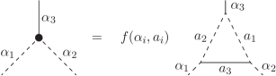
Figure 7: Polyakov conformal triangle for a scalar Yukawa interaction.

The graphs of Figure 6, however, are the lowest order contributions to the full vertex function that we will denote by $V(\bar{y},\alpha,\gamma;\delta,\delta^{\prime})$, where the last two arguments are regularizing parameters. These are required in the derivation of one of the two consistency equations defining the large $N$ bootstrap formalism [29, 30, 31, 44]. The first equation represents Figure 6 and is

$$1=V(\bar{y},\alpha,\gamma;0,0),$$ (6.1)

where $\bar{y}$ is similar to the early amplitude combination $y$ but includes the normalization of the Polyakov conformal triangle of Figure 7. Indeed (6.1) is responsible for determining the terms in the $1/N$ expansion of $\bar{y}$ once the first few orders of $\eta$ have been reproduced in this formalism. This is because the explicit expressions are necessary to extract $\eta_{3}$ from the third order term of the second bootstrap equation which is

$$\frac{T_{F}Nr(\alpha-1)}{C_{F}p(\gamma)}=\frac{\big{[}1+2\chi_{\pi}\frac{\partial}{\partial\delta^{\prime}}V(\bar{y},\alpha,\gamma;\delta,\delta^{\prime})\big{]}}{\big{[}1+2\chi_{\pi}\frac{\partial}{\partial\delta}V(\bar{y},\alpha,\gamma;\delta,\delta^{\prime})\big{]}}\bigg{|}_{\delta=\delta^{\prime}=0}.$$ (6.2)

We note briefly that the regularizations $\delta$ and $\delta^{\prime}$ that appear here arise because of singularities in the $2$-point Schwinger–Dyson equations when all the vertices are replaced by conformal triangles. In other words it was recognised in the original work of [7] that in the absence of any regularization the $2$-point functions with dressed vertices would be finite overall. However each of the contributing diagrams were individually divergent. To accommodate this, and similar to the introduction of $\Delta$ earlier, the vertex anomalous dimension has to be continued in a parallel way to (3.2). This is illustrated in Figure 8 for the leading order contribution to $V(\bar{y},\alpha,\gamma;\delta,\delta^{\prime})$, where we have set

$$\chi_{\pi}=2\tilde{\Delta}_{\pi}$$

for shorthand. This figure indicates the values of the exponents of the internal lines of the Polyakov triangle. Moreover the appearance of both $\delta$ and $\delta^{\prime}$ on the external legs of the graph on the left hand side indicate the addition of the regularizations to the exponents of the respective fields. This is reflected internally in the conformal triangles in the right hand graph as each of the vertices have to be unique even when there is a regularization.

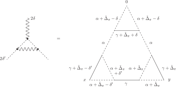
Figure 8: Regularized one loop contribution to the vertex bootstrap equations.

Given the form of (6.2) we can rederive $\eta_{2}$ from knowledge of the value of the graph of Figure 8. This was determined in [15], using the technique given in [44], for the Ising Gross–Neveu model as a function of the exponents of that theory and that result can be translated to (2.3). If we expand $V(\bar{y},\alpha,\gamma;\delta,\delta^{\prime})$ in large $N$ in the same notation as (2.7) then to the order that will eventually be necessary to evaluate $\eta_{3}$ we recall [15]

$$V_{1}=-\frac{Q^{3}}{\tilde{\Delta}_{\pi}\big{(}\tilde{\Delta}_{\pi}-\delta\big{)}\big{(}\tilde{\Delta}_{\pi}-\delta^{\prime}\big{)}}\exp\big{[}F(\delta,\delta^{\prime},\tilde{\Delta}_{\pi})\big{]}$$

with

$$Q=-\frac{a^{2}(\alpha-1)a(\gamma)}{(\alpha-1)^{2}\Gamma(\mu)}$$

and

$$F\big{(}\delta,\delta^{\prime},\tilde{\Delta}_{\pi}\big{)}=\bigg{[}5B_{\gamma}-2B_{\alpha-1}-3B_{0}-\frac{2}{\alpha-1}\bigg{]}\tilde{\Delta}_{\pi}-[B_{\gamma}-B_{0}]\delta$$

$$\hphantom{F\big{(}\delta,\delta^{\prime},\tilde{\Delta}_{\pi}\big{)}=}{}+\bigg{[}B_{0}-B_{\alpha-1}-\frac{1}{\alpha-1}\bigg{]}\delta^{\prime}+\bigg{[}C_{\alpha-1}-\frac{1}{\alpha-1}\bigg{]}\delta\delta^{\prime}$$

$$\hphantom{F\big{(}\delta,\delta^{\prime},\tilde{\Delta}_{\pi}\big{)}=}{}+\bigg{[}C_{\gamma}+C_{0}-2C_{\alpha-1}+\frac{2}{(\alpha-1)^{2}}\bigg{]}\tilde{\Delta}_{\pi}\delta{}+\frac{1}{2}\bigg{[}\frac{1}{(\alpha-1)^{2}}-C_{\alpha-1}-C_{0}\bigg{]}{\delta^{\prime}}^{2}$$

$$\hphantom{F\big{(}\delta,\delta^{\prime},\tilde{\Delta}_{\pi}\big{)}=}+\bigg{[}C_{0}-C_{\gamma}-2C_{\alpha-1}+\frac{2}{(\alpha-1)^{2}}\bigg{]}\tilde{\Delta}_{\pi}\delta^{\prime}-\frac{1}{2}[C_{\gamma}+C_{0}]\delta^{2}$$

$$\hphantom{F(\delta,\delta^{\prime},\tilde{\Delta}_{\pi})=}{}+\bigg{[}C_{\alpha-1}-\frac{7}{2}C_{\gamma}-\frac{3}{2}C_{0}-\frac{1}{(\alpha-1)^{2}}\bigg{]}\tilde{\Delta}_{\pi}^{2}+O\big{(}\tilde{\Delta}_{\pi}^{3},\delta^{3},{\delta^{\prime}}^{3}\big{)},$$ (6.3)

where the order symbol indicates that terms cubic in any combination of the parameters are neglected. The functions $B_{z}$ and $C_{z}$ are defined by [44]

$$B_{z}=\psi(\mu-z)+\psi(z),\qquad B_{0}=\psi(1)+\psi(\mu),$$

$$C_{z}=\psi^{\prime}(z)-\psi^{\prime}(\mu-z),\qquad C_{0}=\psi^{\prime}(\mu)-\psi^{\prime}(1)$$

in terms of the Euler $\psi$ function. With (6.3) and setting $V=V_{1}/N$ in (6.1) and (6.2) it is straightforward to expand both bootstrap equations to $O(1/N)$ and verify the earlier expressions for $\eta_{1}$ and $\eta_{2}$.

Having established the formalism reproduces available results the extension to the next order to find $\eta_{3}$ requires several steps. The first is to compute the next term in the $1/N$ expansion of (6.3) as that will contribute to the $O\big{(}1/N^{2}\big{)}$ part of (6.2). However contributions from all the graphs of Figure 6 bar the one loop one have to be determined and included as they correspond to $V_{2}$. The relevant parts of these graphs were calculated in [15]. By this we mean that a computational shortcut was used akin to that used in [44]. From examining the terms in the formal Taylor expansion of (6.2) in powers of $1/N$ the part involving $V_{2}$ occurs in the combination

$$\bigg{[}\frac{\partial}{\partial\delta^{\prime}}V_{2}(y,\alpha,\gamma;\delta,\delta^{\prime})-\frac{\partial}{\partial\delta}V_{2}(y,\alpha,\gamma;\delta,\delta^{\prime})\bigg{]}\bigg{|}_{\delta=\delta^{\prime}=0}.$$ (6.4)

In [15] the contribution to (6.4) from each of the higher order correction graphs in Figure 6 were determined. Indeed in most cases only the value for the difference in derivatives could be found. Appending the group theory values from the color.h routine allows us to finally extract $\eta_{3}$. We find

$$\eta_{3}=\bigg{[}\frac{(2\mu-1)\big{(}35\mu^{3}-43\mu^{2}+16\mu-2\big{)}}{4\mu^{2}(\mu-1)^{4}}C_{F}^{2}-\frac{\mu^{2}\big{(}43\mu^{2}-35\mu+6\big{)}}{8\mu^{2}(\mu-1)^{4}}C_{F}C_{A}$$

$$\hphantom{\eta_{3}=\bigg{[}}{}-\frac{\mu^{4}\big{(}4\mu^{3}-5\mu^{2}-9\mu-14\big{)}}{48\mu^{2}(\mu-1)^{4}}C_{A}^{2}-\frac{\mu^{4}\big{(}4\mu^{3}-2\mu^{2}-3\mu+10\big{)}}{4\mu^{2}(\mu-1)^{4}}\frac{d_{F}^{abcd}d_{F}^{abcd}}{T_{F}^{2}N_{A}}$$

$$\hphantom{\eta_{3}=\bigg{[}}{}+\bigg{[}\frac{1}{2}(11\mu-3)(2\mu-1)^{2}-\frac{1}{4}\mu(19\mu-2)(2\mu-1)C_{F}C_{A}-\frac{1}{24}\mu^{3}\big{(}2\mu^{2}-6\mu-23\big{)}C_{A}^{2}$$

$$\hphantom{\eta_{3}=\bigg{[}+\bigg{[}}{}-\frac{\mu^{3}\big{(}2\mu^{2}-3\mu+4\big{)}d_{F}^{abcd}d_{F}^{abcd}}{2T_{F}^{2}N_{A}}\bigg{]}\frac{\Psi(\mu)}{\mu(\mu-1)^{3}}$$

$$\hphantom{\eta_{3}=\bigg{[}}{}+\frac{3(2C_{F}-4\mu C_{F}+\mu C_{A})^{2}}{8(\mu-1)^{2}}\Psi^{2}(\mu)+\frac{(2C_{F}-4\mu C_{F}+\mu C_{A})^{2}}{8(\mu-1)^{2}}\Phi(\mu)$$

$$\hphantom{\eta_{3}=\bigg{[}}{}+\bigg{[}(2\mu-1)(\mu+1)C_{F}^{2}-\frac{1}{2}\mu(5\mu-1)C_{F}C_{A}-\frac{1}{24}\mu^{2}(\mu-4)C_{A}^{2}$$

$$\hphantom{\eta_{3}=\bigg{[}+\bigg{[}}{}+\mu^{2}(\mu+8)\frac{d_{F}^{abcd}d_{F}^{abcd}}{T_{F}^{2}N_{A}}\bigg{]}\bigg{[}\Theta(\mu)+\frac{1}{(\mu-1)^{2}}\bigg{]}\frac{1}{4(\mu-1)^{2}}$$

$$\hphantom{\eta_{3}=\bigg{[}}{}-\bigg{[}C_{A}^{2}-24\frac{d_{F}^{abcd}d_{F}^{abcd}}{N_{A}T_{F}^{2}}\bigg{]}\bigg{[}\Theta(\mu)+\frac{1}{(\mu-1)^{2}}\bigg{]}[2\Psi(\mu)+\Xi(\mu)]\frac{\mu^{2}}{16(\mu-1)}\bigg{]}\frac{\eta_{1}^{3}}{C_{F}^{2}}.$$

Again the pieces arising from the light-by-light graphs can be clearly identified. In addition to the Euler $\psi$ function and its derivatives a new function arises which is related to the function $I(\mu)$ defined in [44]. It corresponds to the derivative of a two loop self-energy graph, where a regularizing exponent of one of the propagators is differentiated. In [24] this master graph was expressed in terms of an ${}_{4}F_{3}$ hypergeometric function where the regularizing parameter appears in the parameter arguments of the function. A compact expression for $I(\mu)$ that is valid in $d$-dimensions was recorded in [4]. Here we have set

$$I(\mu)=-\frac{2}{3(\mu-1)}+\Xi(\mu),$$

so that $\Xi(\mu)$ has an $\epsilon$ expansion involving multiple zeta values [3, 24, 44]. For instance,

$$\Xi(1-\epsilon)=\frac{2}{3}\zeta_{3}\epsilon^{2}+\zeta_{4}\epsilon^{3}+\frac{13}{3}\zeta_{5}\epsilon^{4}+O\big{(}\epsilon^{5}\big{)}.$$

In strictly three dimensions [44]

$$I\bigg{(}\frac{3}{2}\bigg{)}=2\ln 2+\frac{3\psi^{\prime\prime}\big{(}\mbox{\small{$\frac{1}{2}$}}\big{)}}{2\pi^{2}}$$

and the expansion around three dimensions is known up to ten terms [5].

7 Results

We focus in this section on general aspects of the critical exponents of (2.3) that we have determined. One of the main reasons for considering a generalized universality class was the fact that known results for specific models could be extracted as well as be of use where a different Lie group underlies the physics problem. To assist with that we have collected electronic expressions in an attached data file. One aspect of the results that needs to be stated is that we have checked that the $d$-dimensional exponents are in agreement with several models where the results were determined directly. For instance, the original Ising Gross–Neveu model of [48] corresponds to the abelian limit of the symmetry group by specifying

$$C_{F}=1,\qquad T_{F}=1,\qquad d_{F}^{abcd}d_{F}^{abcd}=1,\qquad C_{A}=0$$

while the Mott insulating phase [2, 20] that corresponds to taking the symmetry group to be ${\rm SU}(2)$ takes the values

$$C_{F}=\frac{3}{4},\qquad T_{F}=\frac{1}{2},\qquad d_{F}^{abcd}d_{F}^{abcd}=\frac{5}{64},\qquad C_{A}=2.$$

For the more recent application of (2.3) to the fractionalized Gross–Neveu model discussed in [35] the respective values are

$$C_{F}=2,\qquad T_{F}=2,\qquad d_{F}^{abcd}d_{F}^{abcd}=\frac{20}{3},\qquad C_{A}=2.$$

For each of these cases the $\epsilon$ expansion of the exponents near four dimensions with $d=4-2\epsilon$ are in full agreement with known three and four loop perturbative results [9, 21, 23, 27, 32, 35, 52, 53]. In the case of the Ising Gross–Neveu model exponents these also are in accord with two dimensional perturbation theory [10, 12, 16, 18, 25, 26, 47]. Moreover taking the limits for the three cases, all the large $N$ exponents agree with previous work [8, 11, 13, 14, 17, 32, 34, 39, 45].

One advantage of the arbitrary group approach in $d$-dimensions means that the structure of the exponents can be studied in various representations. For example if we restrict the fermions to be in the adjoint representation $A$ whence $C_{F}=C_{A}$ and $T_{F}=C_{A}$. In that case we find

$$\eta_{2}^{\rm adj}=\bigg{[}\frac{13\mu^{2}-12\mu+2}{4\mu[\mu-1]^{2}}+\frac{3\mu-2}{2[\mu-1]}\Psi(\mu)\bigg{]}\big{(}\eta_{1}^{\rm adj}\big{)}^{2},$$

$$\chi_{\pi\,1}^{\rm adj}=\frac{\mu}{2[\mu-1]}\eta_{1}^{\rm adj},$$

$$\chi_{\pi\,2}^{\rm adj}=\bigg{[}\bigg{[}\frac{3\mu^{2}}{\mu-1}\frac{d_{A}^{abcd}d_{A}^{abcd}}{C_{A}^{4}N_{A}}-\frac{\mu^{2}}{8[\mu-1]}\bigg{]}\Theta(\mu)+\frac{\mu(3\mu-2)}{4[\mu-1]^{2}}\Psi(\mu)$$

$$\hphantom{\chi_{\pi\,2}^{\rm adj}=\bigg{[}\bigg{[}}{}-\frac{\mu(\mu+1)(\mu-3)}{6[\mu-1]^{2}}-\frac{\mu^{2}(2\mu-1)}{[\mu-1]^{2}}\frac{d_{A}^{abcd}d_{A}^{abcd}}{C_{A}^{4}N_{A}}\bigg{]}\big{(}\eta_{1}^{\rm adj}\big{)}^{2},$$

$$\lambda_{2}^{\rm adj}=\bigg{[}\bigg{[}\frac{1}{6}\mu\big{(}3\mu^{2}-6\mu+2\big{)}+4\mu\frac{d_{A}^{abcd}d_{A}^{abcd}}{C_{A}^{4}N_{A}}\bigg{]}\frac{1}{[\mu-1][\mu-2]^{2}\eta_{1}^{\rm adj}}$$

$$\hphantom{\lambda_{2}^{\rm adj}=\bigg{[}}{}-\bigg{[}\frac{1}{24}\mu^{2}(2\mu-3)+2\mu^{2}(2\mu-3)\frac{d_{A}^{abcd}d_{A}^{abcd}}{C_{A}^{4}N_{A}}\bigg{]}\frac{\Psi^{2}(\mu)+\Phi(\mu)}{[\mu-1][\mu-2]}$$

$$\hphantom{\lambda_{2}^{\rm adj}=\bigg{[}}{}-\bigg{[}\frac{1}{24}(\mu-1)\big{(}96\mu^{5}-438\mu^{4}+549\mu^{3}+4\mu^{2}-288\mu+96\big{)}$$

$$\hphantom{\lambda_{2}^{\rm adj}=\bigg{[}{-}\bigg{[}}{}+\mu^{2}(3\mu-5)(2\mu-5)\frac{d_{A}^{abcd}d_{A}^{abcd}}{C_{A}^{4}N_{A}}\bigg{]}\frac{\Psi(\mu)}{[\mu-1]^{2}[\mu-2]^{2}}$$

$$\hphantom{\lambda_{2}^{\rm adj}=\bigg{[}}{}+\bigg{[}3\mu^{2}(5\mu-7)\frac{d_{A}^{abcd}d_{A}^{abcd}}{C_{A}^{4}N_{A}}-\frac{1}{8}\mu^{2}(\mu-2)(12\mu-7)\bigg{]}\frac{\Theta(\mu)}{[\mu-1][\mu-2]}$$

$$\hphantom{\lambda_{2}^{\rm adj}=\bigg{[}}{}+\frac{192\mu^{8}-1544\mu^{7}+4770\mu^{6}-6865\mu^{5}+3951\mu^{4}+724\mu^{3}-1896\mu^{2}+768\mu-96}{48\mu[\mu-1]^{3}[\mu-2]^{2}}$$

$$\hphantom{\lambda_{2}^{\rm adj}=\bigg{[}}{}-\frac{\mu^{2}\big{(}4\mu^{4}-18\mu^{3}+26\mu^{2}-15\mu+7\big{)}}{2[\mu-1]^{3}[\mu-2]^{2}}\frac{d_{A}^{abcd}d_{A}^{abcd}}{C_{A}^{4}N_{A}}\bigg{]}\big{(}\eta_{1}^{\rm adj}\big{)}^{2},$$

$$\eta_{3}^{\rm adj}=\bigg{[}\frac{(3\mu-2)^{2}}{8[\mu-1]^{2}}[\Phi(\mu)+3\Psi^{2}(\mu)]-\frac{\mu^{2}(2\mu-1)(\mu^{2}-1)}{2[\mu-1]^{4}}\frac{d_{A}^{abcd}d_{A}^{abcd}}{C_{A}^{4}N_{A}}$$

$$\hphantom{\eta_{3}^{\rm adj}=\bigg{[}}{}-\frac{8\mu^{7}-10\mu^{6}-17\mu^{5}-1184\mu^{4}+2448\mu^{3}-1704\mu^{2}+480\mu-48}{96\mu^{2}[\mu-1]^{4}}$$

$$\hphantom{\eta_{3}^{\rm adj}=\bigg{[}}{}-\bigg{[}\frac{1}{12}\big{(}\mu^{5}-3\mu^{4}-160\mu^{3}+267\mu^{2}-132\mu+18\big{)}$$

$$\hphantom{\eta_{3}^{\rm adj}=\bigg{[}{-}\bigg{[}}{}+\frac{1}{2}\mu^{3}(2\mu+1)(\mu-2)\frac{d_{A}^{abcd}d_{A}^{abcd}}{C_{A}^{4}N_{A}}\bigg{]}\frac{\Psi(\mu)}{\mu[\mu-1]^{3}}$$

$$\hphantom{\eta_{3}^{\rm adj}=\bigg{[}}{}+\bigg{[}\frac{1}{4}\mu^{2}(\mu+8)\frac{d_{A}^{abcd}d_{A}^{abcd}}{C_{A}^{4}N_{A}}-\frac{1}{96}(\mu^{3}+8\mu^{2}-36\mu+24)\bigg{]}\frac{\Theta(\mu)}{[\mu-1]^{2}}$$

$$\hphantom{\eta_{3}^{\rm adj}=\bigg{[}}{}-\frac{\mu^{2}}{8[\mu-1]}\bigg{[}1-24\frac{d_{A}^{abcd}d_{A}^{abcd}}{C_{A}^{4}N_{A}}\bigg{]}\Theta(\mu)\Psi(\mu)-\frac{\mu^{2}\Xi(\mu)}{16[\mu-1]^{3}}\bigg{[}1-24\frac{d_{A}^{abcd}d_{A}^{abcd}}{C_{A}^{4}N_{A}}\bigg{]}$$

$$\hphantom{\eta_{3}^{\rm adj}=\bigg{[}}{}-\frac{\mu^{2}}{16[\mu-1]}\bigg{[}1-24\frac{d_{A}^{abcd}d_{A}^{abcd}}{C_{A}^{4}N_{A}}\bigg{]}\Xi(\mu)\Theta(\mu)\bigg{]}\big{(}\eta_{1}^{\rm adj}\big{)}^{3},$$

where $d_{A}^{abcd}$ is the adjoint version of the fully symmetric rank $4$ Casimir. These exponents simplify substantially in three dimensions since

$$\lambda\big{|}_{d=3}=1-\frac{16}{3\pi^{2}N}+\bigg{[}96\frac{d_{A}^{abcd}d_{A}^{abcd}}{C_{A}^{4}N_{A}}+\frac{5248}{\pi^{2}}-432\bigg{]}\frac{1}{27\pi^{2}N^{2}},$$

$$\eta\big{|}_{d=3}=\frac{8}{3\pi^{2}N}+\frac{1216}{27\pi^{4}N^{2}}+\big{[}\big{[}9072\zeta_{3}-864\pi^{2}\ln 2\big{]}\big{[}C_{A}^{4}N_{A}-24d_{A}^{abcd}d_{A}^{abcd}\big{]}$$

$$\hphantom{\eta\big{|}_{d=3}=}{}+\big{[}25920\pi^{2}-435456\big{]}d_{A}^{abcd}d_{A}^{abcd}+\big{[}151072-8760\pi^{2}\big{]}C_{A}^{4}N_{A}\big{]}\frac{1}{243\pi^{6}C_{A}^{4}N_{A}N^{3}}.$$

The group valued coefficient of the terms involving $\zeta_{3}$ and $\pi^{2}\ln 2$, which derive from $I\big{(}\mbox{\small{$\frac{3}{2}$}}\big{)}$, has an interesting combination of Casimirs. Indeed there might be instances of this factor being zero for certain Lie groups. However, we have computed the value of $\big{(}C_{A}^{4}N_{A}-24d_{A}^{abcd}d_{A}^{abcd}\big{)}$ for all the classical and exceptional Lie groups and found that it is always non-zero.

8 Discussion

As the Ising Gross–Neveu universality class is central to a number of phase transitions in various materials, we have examined a generalized version of the underlying quantum field theory that incorporates the respective condensed matter systems. The key aspect is that the core interaction is endowed with a non-abelian symmetry that has a parallel in gauge theories. There the gauge interaction of QED is extended from an abelian to a non-abelian one to produce QCD by the inclusion of the generators of a Lie group thereby endowing QED with a colour symmetry. The similar extension of the Ising Gross–Neveu model is simpler in some respects. One obvious one is the absence of gauge symmetry. A benefit, however, is that considering (2.3) at the outset means results for specific phase transitions can be quickly deduced by specifying the Lie group. Indeed if a phase transition were discovered in a material that was in the same universality class as the Ising Gross–Neveu model but possessed a new symmetry other than the specific examples we have noted here, then information on the exponents can readily be deduced from our results. Throughout we have focussed on the application of the critical point large $N$ technique developed in [42, 43, 44] to determine $d$-dimensional critical exponents. The advantage of this is that results are available for the renormalization group functions of the four dimensional quantum field theories in the same universality class too. By the same token the large $N$ exponents contain a wealth of information on the structure of the same functions. For instance, coefficients in the anomalous dimension beyond the first few known loop orders can be accessed at successive orders in $1/N$. This is particularly useful in that our $O\big{(}1/N^{2}\big{)}$ and $O\big{(}1/N^{3}\big{)}$ exponents can reveal where the new colour group Casimirs, such as $d_{F}^{abcd}d_{F}^{abcd}$, appear. In indicating the parallel of the QED to QCD generalization, examining the large $N$ $O\big{(}1/N^{2}\big{)}$ exponents in this universality class, albeit with a simpler vertex structure, does provide useful insight into what to expect in the calculation of critical exponents in QCD at $O\big{(}1/N^{2}\big{)}$. We have to qualify this comment by noting that while there are similarities, in the QCD large $N$ critical exponent computation for $\nu$ for instance, there will be more graphs to consider than those of Figure 5. This is because in (2.3) Feynman diagrams with subgraphs involving three $\pi^{a}$ lines connecting to a fermion loop are zero after taking the $\gamma$-matrix trace. In QCD this would not be the case due to each vertex adding an extra $\gamma$-matrix to the trace. While such graphs remain to be computed the associated group theory factor that would result should not involve any Casimir higher than $d_{F}^{abcd}d_{F}^{abcd}$.

Acknowledgements

This work was fully supported by a DFG Mercator Fellowship and in part with the STFC Consolidated ST/T000988/1. The graphs were drawn with the Axodraw package [6]. Computations were carried out in part using the symbolic manipulation language Form [37, 46].

References

- [1] Ashkin J., Teller E., Statistics of two-dimensional lattices with four components, Phys. Rev. 64 (1943), 178–184.
- [2] Assaad F.F., Herbut I.F., Pinning the order: the nature of quantum criticality in the Hubbard model on honeycomb lattice, Phys. Rev. X 3 (2013), 031010, 8 pages, arXiv:1304.6340.
- [3] Bierenbaum I., Weinzierl S., The massless two-loop two-point function, Eur. Phys. J. C 32 (2003), 67–78, arXiv:hep-ph/0308311.
- [4] Broadhurst D.J., Gracey J.A., Kreimer D., Beyond the triangle and uniqueness relations: non-zeta counterterms at large from positive knots, Z. Phys. C 75 (1997), 559–574, arXiv:hep-th/9607174.
- [5] Broadhurst D.J., Kotikov A.V., Compact analytical form for non-zeta terms in critical exponents at order , Phys. Lett. B 441 (1998), 345–353, arXiv:hep-th/9612013.
- [6] Collins J.C., Vermaseren J.A.M., Axodraw Version 2, arXiv:1606.01177.
- [7] D’eramo M., Peliti L., Parisi G., Theoretical predictions for critical exponents at the -point of bose liquids, Lett. Nuovo Cimento 2 (1971), 878–880.
- [8] Derkachov S.É., Kivel N.A., Stepanenko A.S., Vasil’ev A.N., On calculation in expansions of critical exponents in the Gross–Neveu model with the conformal technique, arXiv:hep-th/9302034.
- [9] Fei L., Giombi S., Klebanov I.R., Tarnopolsky G., Yukawa CFTs and emergent supersymmetry, Progr. Theoret. Exp. Phys. 2016 (2016), 12C105, 32 pages, arXiv:1607.05316.
- [10] Gracey J.A., Three loop calculations in the Gross–Neveu model, Nuclear Phys. B 341 (1990), 403–418.
- [11] Gracey J.A., Calculation of exponent to in the Gross Neveu model, Internat. J. Modern Phys. A 6 (1991), 395–407, Erratum, Internat. J. Modern Phys. A 6 (1991), 2755.
- [12] Gracey J.A., Computation of the three-loop -function of the Gross–Neveu model in minimal subtraction, Nuclear Phys. B 367 (1991), 657–674.
- [13] Gracey J.A., Anomalous mass dimension at in the Gross–Neveu model, Phys. Lett. B 297 (1992), 293–297.
- [14] Gracey J.A., Computation of at in the Gross–Neveu model in arbitrary dimensions, Internat. J. Modern Phys. A 9 (1994), 567–589, arXiv:hep-th/9306106.
- [15] Gracey J.A., Computation of critical exponent at in the four-fermi model in arbitrary dimensions, Internat. J. Modern Phys. A 9 (1994), 727–744, arXiv:hep-th/9306107.
- [16] Gracey J.A., Four loop mass anomalous dimension in the Gross–Neveu model, Nuclear Phys. B 802 (2008), 330–350, arXiv:0804.1241.
- [17] Gracey J.A., Large critical exponents for the chiral Heisenberg Gross–Neveu universality class, Phys. Rev. D 97 (2018), 105009, 17 pages, arXiv:1801.01320.
- [18] Gracey J.A., Luthe T., Schröder Y., Four loop renormalization of the Gross–Neveu model, Phys. Rev. D 94 (2016), 125028, 18 pages, arXiv:1609.05071.
- [19] Gross D.J., Neveu A., Dynamical symmetry breaking in asymptotically free field theories, Phys. Rev. D 10 (1974), 3235–3253.
- [20] Herbut I.F., Juric̆ić V., Vafek O., Relativistic Mott criticality in graphene, Phys. Rev. B 80 (2009), 075432, 4 pages, arXiv:0904.1019.
- [21] Ihrig B., Mihaila L.N., Scherer M.M., Critical behavior of Dirac fermions from perturbative renormalization, Phys. Rev. B 98 (2018), 125109, 20 pages, arXiv:1806.04977.
- [22] Janssen L., Herbut I.F., Antiferromagnetic critical point on graphene’s honeycomb lattice: A functional renormalization group approach, Phys. Rev. B 89 (2014), 205403, 14 pages, arXiv:1402.6277.
- [23] Kärkkäinen L., Lacaze R., Lacock P., Petersson B., Critical behavior of the three-dimensional Gross–Neveu and Higgs–Yukawa models, Nuclear Phys. B 415 (1994), 781–796, arXiv:hep-lat/9310020.
- [24] Kotikov A.V., The Gegenbauer polynomial technique: the evaluation of a class of Feynman diagrams, Phys. Lett. B 375 (1996), 240–248, arXiv:hep-ph/9512270.
- [25] Ludwig A.W.W., Critical behavior of the two-dimensional random -state Potts model by expansion in , Nuclear Phys. B 285 (1987), 97–142.
- [26] Luperini C., Rossi P., Three-loop function(s) and effective potential in the Gross–Neveu model, Ann. Physics 212 (1991), 371–401.
- [27] Mihaila L.N., Zerf N., Ihrig B., Herbut I.F., Scherer M.M., Gross–Neveu–Yukawa model at three loops and Ising critical behavior of Dirac systems, Phys. Rev. B 96 (2017), 165133, 6 pages, arXiv:1703.08801.
- [28] Parisi G., On self-consistency conditions in conformal covariant field theory, Lett. Nuovo Cimento 4 (1972), 777–780.
- [29] Parisi G., Peliti L., Calculation of critical indices, Lett. Nuovo Cimento 2 (1971), 627–628.
- [30] Polyakov A.M., Microscopic description of critical phenomena, Sov. Phys. JETP 28 (1969), 533–539.
- [31] Polyakov A.M., Conformal symmetry of critical fluctuations, JETP Lett. 12 (1970), 381–383.
- [32] Ray S., Ihrig B., Kruti D., Gracey J.A., Scherer M.M., Janssen L., Fractionalized quantum criticality in spin-orbital liquids from field theory beyond the leading order, Phys. Rev. B 103 (2021), 155160, 18 pages, arXiv:2101.10335.
- [33] Rosenstein B., Warr B.J., Park S.H., Four-fermion theory is renormalizable in 2+1 dimensions, Phys. Rev. Lett. 62 (1989), 1433–1436.
- [34] Rosenstein B., Warr B.J., Park S.H., Dynamical symmetry breaking in four-fermion interaction models, Phys. Rep. 205 (1991), 59–108.
- [35] Seifert U.F.P., Dong X.Y., Chulliparambil S., Vojta M., Tu H.H., Janssen L., Fractionalized fermionic quantum criticality in spin-orbital Mott insulators, Phys. Rev. Lett. 125 (2020), 257202, 7 pages, arXiv:2009.05051.
- [36] Sorella S., Otsuka Y., Yunoki S., Absence of a spin liquid phase in the Hubbard model on the honeycomb lattice, Sci. Rep. 2 (2012), 992, 5 pages, arXiv:1207.1783.
- [37] Tentyukov M., Vermaseren J.A.M., The multithreaded version of FORM, Comput. Phys. Comm. 181 (2010), 1419–1427, arXiv:hep-ph/0702279.
- [38] van Ritbergen T., Schellekens A.N., Vermaseren J.A.M., Group theory factors for Feynman diagrams, Internat. J. Modern Phys. A 14 (1999), 41–96, arXiv:hep-ph/9802376.
- [39] Vasil’ev A.N., Derkachov S.É., Kivel N.A., Stepanenko A.S., The expansion in the Gross–Neveu model: conformal bootstrap calculation of the index in order , Theoret. and Math. Phys. 94 (1993), 127–136.
- [40] Vasil’ev A.N., Nalimov M.Yu., Analog of dimensional regularization for calculation of the renormalization group functions in the expansion for arbitrary dimension of space, Theoret. and Math. Phys. 55 (1983), 423–431.
- [41] Vasil’ev A.N., Nalimov M.Yu., The model: calculation of anomalous dimensions and the mixing matrices in the order , Theoret. and Math. Phys. 56 (1983), 643–653.
- [42] Vasil’ev A.N., Pismak Yu.M., Honkonen J.R., expansion: calculation of the exponents and in the order for arbitrary number of dimensions, Theoret. and Math. Phys. 47 (1981), 465–475.
- [43] Vasil’ev A.N., Pismak Yu.M., Honkonen J.R., Simple method of calculating the critical indices in the expansion, Theoret. and Math. Phys. 46 (1981), 104–113.
- [44] Vasil’ev A.N., Pismak Yu.M., Honkonen J.R., expansion: calculation of the exponent in the order by the conformal bootstrap method, Theoret. and Math. Phys. 50 (1982), 127–134.
- [45] Vasil’ev A.N., Stepanenko A.S., -expansion in the Gross–Neveu model: calculation of the index to the order by the conformal bootstrap method, Theoret. and Math. Phys. 97 (1993), 1349–1354.
- [46] Vermaseren J.A.M., New features of FORM, arXiv:math-ph/0010025.
- [47] Wetzel W., Two-loop -function for the Gross–Neveu model, Phys. Lett. B 153 (1985), 297–299.
- [48] Wilson K.G., Renormalization group and critical phenomena. II. Phase-space cell analysis of critical behavior, Phys. Rev. B 4 (1971), 3184–3205.
- [49] Wilson K.G., Feynman graph expansion for critical exponents, Phys. Rev. Lett. 28 (1972), 548–551.
- [50] Wilson K.G., Fisher M.E., Critical exponents in 3.99 dimensions, Phys. Rev. Lett. 28 (1972), 240–243.
- [51] Wilson K.G., Kogut J., The renormalization group and the expansion, Phys. Rep. 12 (1974), 75–199.
- [52] Zerf N., Mihaila L.N., Marquard P., Herbut I.F., Scherer M.M., Four-loop critical exponents for the Gross–Neveu–Yukawa models, Phys. Rev. D 96 (2017), 096010, 19 pages, arXiv:1709.05057.
- [53] Zinn-Justin J., Four-fermion interaction near four dimensions, Nuclear Phys. B 367 (1991), 105–122.