BGK models for inert mixtures: comparison and applications

Abstract.

Consistent BGK models for inert mixtures are compared, first in their kinetic behavior and then versus the hydrodynamic limits that can be derived in different collision-dominated regimes. The comparison is carried out both analytically and numerically, for the latter using an asymptotic preserving semi-Lagrangian scheme for the BGK models. Application to the plane shock wave in a binary mixture of noble gases is also presented.

1. Introduction

Since the seminal paper of Bhatnagar, Gross and Krook [10], BGK models of the Boltzmann equation [14, 28] play the role of simpler and effective modeling tools to describe the dynamics of rarefied gases. Their importance is much more evident when gas mixtures are taken into account. However, the extension to an arbitrary mixture of monoatomic gases is not trivial, since interactions and exchanges between different components, as well as conservation of total momentum and energy, must be properly considered.
The first mathematically rigorous contribution appeared in [2], where the authors proposed a BGK model characterized by a single global operator for each species, able to reproduce the correct exchange rates for momemtum and kinetic energy among species of the Boltzmann equations for mixtures, assuming intermolecular potentials of Maxwell molecules type. Later, several BGK models have been introduced, characterized by different structures of the BGK operators (see for instance [24, 26, 27] and the reference therein). In [22] the authors consider a BGK model for inert mixtures whose single global collision operator for each species allows to correctly reproduce the conservation of total momentum and kinetic energy; moreover, in the same paper a comparison among this BGK model and the one proposed in [2] is presented and discussed. For both BGK models in [2] and [22] the possibility to include simple chemical reactions has been considered, and their extension to bimolecular chemical reactions in mixtures of monoatomic gases can be found in [23] and [6, 19], respectively.
Recently, in [11] a further different consistent BGK-type model is built up, that mimics the structure of the Boltzmann equations for mixtures, namely in which the collision operator for each species is a sum of bi-species BGK operators. This last model is consistent and well–posed as the one in [2], but in addition allows to deal with general intermolecular potentials. The exchange rates for momentum and energy of each BGK operator coincide by construction with the corresponding exchange rates of each Boltzmann binary integral operator, getting thus exact conservations. The structure of the collision operator in this case allows to consistently derive evolution equations for the main macroscopic fields in different hydrodynamic regimes, according to the dominant collisional phenomenon [3, 4].
This paper is aiming at comparing the behaviors of the above mentioned BGK models for inert mixtures of monoatomic gases in various regimes, from kinetic to hydrodynamic, and to highlight their analogies and discrepancies. In addition, two different Navier-Stokes hydrodynamic limits, characterized by global velocity and temperature or multi-velocity and multi-temperature, respectively, and obtained from the consistent BGK model in [11], are numerically tested with respect to their capability to reproduce the correct dynamics of realistic mixtures of noble gases, with particular attention to the case of mixtures of heavy and light particles (the so called $\varepsilon$-mixtures [18]). For the numerical solutions to BGK models, semi-Lagrangian methods proposed in [15, 22] will be adopted together with a conservative reconstruction technique [12, 13], which enables us to capture the correct behaviors of hydrodynamic limit models. As regards details and properties of semi-Lagrangian schemes (for single gas BGK model), we refer to papers regarding the construction of high order semi-Lagrangian schemes [8, 20, 33], treatment of boundary problems [21, 32] and convergence analysis [9, 34, 35].
The paper is organized as follows. In section 2, we briefly recall the classical Boltzmann equation for inert gas mixtures. Section 3 is devoted to the description of the three BGK models considered in this paper. Next, in section 4, we study analytically the discrepancy between BGK models at the level of collision operators. Then, in section 5, we present hydrodynamic limits at Navier-Stokes level that can be obtained from the kinetic BGK models. In section 6, we perform numerical experiments in which we investigate the discrepancy of the three BGK models, compare them with their two corresponding Navier-Stokes limits, and study the Riemann problem and the steady shock structure in binary mixtures of noble gases, with different mass ratios.

2. Kinetic Boltzmann-Type Equations

Let us consider a mixture of $L$ monoatomic inert gases. Under the assumption that $s$-th gas has a mass $m_{s}>0$, its dynamics can be described through the distribution functions $f_{s}({\bf x},{\bf v},t)$, $s=1,\cdots,L$ defined on phase space $({\bf x},{\bf v})\in\mathbb{R}^{3}\times\mathbb{R}^{3}$ at time $t>0$, whose evolution is governed by the Boltzmann-type equations:

(2.1) $$\frac{\partial{f_{s}}}{\partial t}+{\bf v}\cdot\nabla_{\textbf{x}}f_{s}=Q_{s},$$

where $Q_{s}$ is the collision term of the $s$-th species, which collects bi-species collision operators between $s$-th and other $k$-th gases:

$$Q_{s}=\sum_{k=1}^{N}Q_{sk}(f_{s},f_{k}).$$

The binary collision operator $Q_{sk}$ can be cast as

(2.2) $$Q_{sk}(f_{s},f_{k})=\int_{\mathbb{R}^{3}\times\mathbb{S}^{2}}d{\bf w}\,d{\boldsymbol{\omega}}\,g_{sk}\left(|\bf{y}|,\hat{\bf{y}}\cdot{\boldsymbol{\omega}}\right)\bigg{[}f_{s}({\bf v}^{\prime})f_{k}({\bf w}^{\prime})-f_{s}({\bf v})f_{k}({\bf w})\bigg{]}$$

with a non-negative scattering kernel $g_{sk}$ depending on intermolecular potentials. Here we use the integration variable ${\bf w}\in\mathbb{R}^{3}$, a unit vector on a sphere $\boldsymbol{\omega}\in\mathbb{S}^{2}$, the relative velocity ${\bf y}:={\bf v}-{\bf w}$ and its unit vector $\hat{{\bf y}}:={\bf y}/|{\bf y}|$. The other two variables ${\bf v}^{\prime}$ and ${\bf w}^{\prime}$ are post collisional velocities of $s$-th and $k$-th gases whose masses are $m_{s}$, $m_{k}$ and pre-collisional velocities are ${\bf v}$, ${\bf w}$, respectively:

$${\bf v}^{\prime}=\frac{m_{s}{\bf v}+m_{k}{\bf w}}{m_{s}+m_{k}}+\frac{m_{k}}{m_{s}+m_{k}}|{\bf y}|\boldsymbol{\omega},\quad{\bf w}^{\prime}=\frac{m_{s}{\bf v}+m_{k}{\bf w}}{m_{s}+m_{k}}-\frac{m_{s}}{m_{s}+m_{k}}|{\bf y}|\boldsymbol{\omega}.$$

(for more details, see for instance [14] and references therein).

The distribution function $f_{s}$, $s=1,\dots,L$, can be used to reproduce $s$-species macroscopic quantities such as number density $n_{s}$, average velocity $u_{s}$, absolute temperature $T_{s}$:

$$n_{s}=\langle f_{s},1\rangle,\quad n_{s}u_{s}=\langle f_{s},{\bf v}\rangle,\quad 3n_{s}K_{B}T_{s}=m_{s}\langle f_{s},|{\bf v}-u_{s}|^{2}\rangle$$

where

$$\langle f,h\rangle:=\int_{\mathbb{R}^{3}}dvf({\bf v})h({\bf v}).$$

Similarly, global macroscopic variables such as number density $n$, mass density $\rho$, velocity $u$ and temperature $T$ of the mixture can be obtained as follows:

$$n=\sum_{s=1}^{L}n_{s},\quad\rho=\sum_{s=1}^{L}\rho_{s},\quad\rho_{s}=m_{s}n_{s},\quad s=1,\cdots,L$$

$$u=\frac{1}{\rho}\sum_{s=1}^{L}\rho_{s}u_{s},\quad 3nK_{B}T=3\sum_{s=1}^{L}n_{s}K_{B}T_{s}+\sum_{s=1}^{L}\rho_{s}|u_{s}-u|^{2}$$

The equilibrium solution to (2.1) is given by the Maxwellian which shares a common velocity $u$ and temperature $T$:

$$f_{s}^{eq}=n_{s}M\left({\bf v};u,\frac{K_{B}T}{m_{s}}\right)$$

where

(2.3) $$M\left({\bf v};a,b\right)\equiv\left(\frac{1}{2\pi b}\right)^{3/2}\exp\left(-\frac{1}{2b}\left|{\bf v}-a\right|^{2}\right),\quad a\in\mathbb{R}^{3},\,b>0.$$

The structure of the collision operators $Q_{s}$ allows to guarantee fundamental properties of the Boltzmann equations for inert gas mixtures: conservation laws, uniqueness of equilibrium solutions, H- theorem.

3. BGK-type models

In this section we briefly recall the three different BGK models for eqns. (2.1)-(2.2) which have been compared in this paper.

3.1. The BGK Model of Andries, Aoki and Perthame (AAP model)

In [2], a BGK-type model was proposed, that allows to reproduce the same exchange rate in momentum and energy of the Boltzmann equation (2.1). In this model the collision term $Q_{s}$ (2.2) of the Boltzmann equation is replaced by a relaxation operator which drives the evolution towards an attracting auxiliary Maxwellian $M^{s}$, depending on fictitious parameters. In spite of such structural change, this BGK model still satisfies the main properties of the Boltzmann equation such as conservation law, $H$-theorem, indifferentiability principle. The scaled model equations are described by

(3.1) $$\frac{\partial{f_{s}}}{\partial{t}}+{\bf v}\cdot\nabla_{\textbf{x}}{f_{s}}=\frac{\nu_{s}}{\varepsilon}\left(n_{s}M^{s}-f_{s}\right),\quad s=1,\cdots,L,$$

where $\varepsilon$ is the Knudsen number, $\nu_{s}$ is the collision frequency for $s$-species gas and $M^{s}$ is the attracting Maxwellian:

$$M^{s}=M\left({\bf v};u^{s},\frac{K_{B}T^{s}}{m_{s}}\right),$$

where $M$ is defined in (2.3). Notice that $M^{s}$ is defined in terms of fictitious parameters $u^{s},T^{s}$ (different from the actual fields $u_{s},T_{s}$), which, under the assumption of Maxwell molecules interaction potential, are explicit functions of the actual moments of the distribution function as follows:

(3.2) $$\begin{split}u^{s}&=u_{s}+\frac{1}{m_{s}n_{s}\nu_{s}}\sum_{k=1}^{L}\xi^{sk}u_{k},\cr T^{s}&=T_{s}-\frac{m_{s}}{3K_{B}}\left(|u^{s}|^{2}-|u_{s}|^{2}\right)+\frac{2}{3n_{s}K_{B}\nu_{s}}\sum_{k=1}^{L}\gamma^{sk}T_{k}\cr&\quad+\frac{2}{3n_{s}K_{B}\nu_{s}}\sum_{k=1}^{L}\nu_{1}^{sk}\frac{m_{s}m_{k}n_{s}n_{k}}{(m_{s}+m_{k})^{2}}\left(m_{s}u_{s}+m_{k}u_{k}\right)\left(u_{k}-u_{s}\right),\end{split}$$

where

(3.3) $$\begin{split}\xi_{sk}&=\nu_{1}^{sk}\frac{m_{s}m_{k}n_{s}n_{k}}{m_{s}+m_{k}}-\delta_{sk}\sum_{r=1}^{L}\nu_{1}^{sr}\frac{m_{s}m_{r}n_{s}n_{r}}{m_{s}+m_{r}}\cr\gamma^{sk}&=3K_{B}\nu_{1}^{sk}\frac{m_{s}m_{k}n_{s}n_{k}}{(m_{s}+m_{k})^{2}}-\delta_{sk}\sum_{r=1}^{L}3K_{B}\nu_{1}^{sr}\frac{m_{s}m_{r}n_{s}n_{r}}{(m_{s}+m_{r})^{2}}.\end{split}$$

The collision frequency $\nu_{\ell}^{sk}$ is defined by

$$\nu_{\ell}^{sk}=2\pi|g|\int_{0}^{\pi}g(\omega)(1-\cos\omega)^{\ell}\sin\omega d\omega,$$

and satisfies $\nu_{\ell}^{sk}\leq 2\nu_{0}^{sk}$ for $\ell=1,2$. We remark that this model is well defined with the choice

$$\nu_{s}=\sum_{k=1}^{L}\nu_{0}^{sk}n_{k},$$

which guarantees the positivity of temperature. Moreover, for consistency, we hereafter assume the following case:

(3.4) $$\nu_{0}^{sk}=\nu_{1}^{sk}=:\lambda_{sk}.$$

3.2. The BGK model preserving global conservations (GS model)

Another BGK-type model with one attracting Maxwellian for each species has been proposed in [6, 22]. The fictitious parameters are adjusted to impose the same conservation laws of the Boltzmann equation (2.1), namely species number densities, global momentum, total kinetic energy. In [6, 22], the model has been originally designed to describe a bimolecular reversible chemical reaction in a four species mixture; the model has been then adapted to a general $L$ species inert gas mixture in [22]. The scaled model reads

(3.5) $$\frac{\partial{f_{s}}}{\partial{t}}+{\bf v}\cdot\nabla_{\textbf{x}}{f_{s}}=\frac{\nu_{s}}{\varepsilon}\left(n_{s}M^{s}_{GS}-f_{s}\right).$$

where $\nu_{s}$ is the collision frequency for $s$-species gas and $M^{s}_{GS}$ is the attracting Maxwellian:

(3.6) $$M_{GS}^{s}=M\left({\bf v};\bar{u},\frac{K_{B}\bar{T}}{m_{s}}\right),$$

where $M$ is defined in (2.3). Note that it depends only on the auxiliary parameters $\bar{u}$ and $\bar{T}$, which are determined by imposing the conservation of total momentum and energy:

$$\sum_{s=1}^{L}\int_{\mathbb{R}^{3}}m_{s}\begin{pmatrix}{\bf v}\\ |{\bf v}|^{2}/2\end{pmatrix}\left(n_{s}M^{s}_{GS}-f_{s}\right)\,d{\bf v} =0,$$

Consequently, we obtain the following representation of $\bar{u}$ and $\bar{T}$ in terms of the actual macroscopic fields $u_{s}$ and $T_{s}$:

$$\begin{split}\bar{u}&=\frac{\sum_{s=1}^{L}\nu_{s}m_{s}n_{s}u_{s}}{\sum_{s=1}^{L}\nu_{s}m_{s}n_{s}},\end{split}$$

$$\begin{split}\bar{T}&=\frac{\sum_{s=1}^{L}\nu_{s}n_{s}\left(m_{s}\left(|u_{s}|^{2}-|\bar{u}|^{2}\right)+3K_{B}T_{s}\right)}{3K_{B}\sum_{s=1}^{L}\nu_{s}n_{s}}.\end{split}$$

In [22], it is proved that the positivity of auxiliary temperature $\bar{T}$ is guaranteed and the H-theorem holds for the space homogeneous case.

3.3. A general consistent BGK model for inert gas mixtures (BBGSP model)

In [11], authors introduce a different BGK-type model whose BGK operators $Q_{s}$ mimic the structure of the Boltzmann ones, namely are sums of bi-species operators $Q_{sk}$, each of them prescribing the same exchange rates of the corresponding term of the Boltzmann equations. This model also satisfies the main qualitative properties of Boltzmann equation such as conservation laws, $H$-theorem, indifferentiability principle. The scaled equations read

(3.7) $$\frac{\partial{f_{s}}}{\partial{t}}+{\bf v}\cdot\nabla_{\textbf{x}}{f_{s}}=\frac{1}{\varepsilon}\sum_{k=1}^{L}\nu_{sk}\left(n_{s}M_{sk}-f_{s}\right),\quad s=1,\cdots,L,$$

with

$$M_{sk}=M\left({\bf v};u_{sk},\frac{K_{B}T_{sk}}{m_{s}}\right),$$

where $M$ is defined in (2.3). The auxiliary parameters $u_{sk}$ and $T_{sk}$ are defined by

(3.8) $$\begin{split}u_{sk}&=(1-a_{sk})u_{s}+a_{sk}u_{k}\cr T_{sk}&=(1-b_{sk})T_{s}+b_{sk}T_{k}+\frac{\gamma_{sk}}{K_{B}}\left|u_{s}-u_{k}\right|^{2}\end{split}$$

with

(3.9) $$a_{sk}=\frac{\lambda_{sk}n_{k}m_{k}}{\nu_{sk}(m_{s}+m_{k})},\quad b_{sk}=\frac{2a_{sk}m_{s}}{m_{s}+m_{k}},\quad\gamma_{sk}=\frac{m_{s}a_{sk}}{3}\left(\frac{2m_{k}}{m_{s}+m_{k}}-a_{sk}\right).$$

In [11], authors proved that the positivity of $T_{sk}$ is guaranteed by

$$T_{s}>0,\quad T_{k}>0,\quad\nu_{sk}\geq\frac{1}{2}\lambda_{sk}n_{k}.$$

Considering this, throughout this paper, we set $\nu_{sk}=\nu_{0}^{sk}n_{k}=\lambda_{sk}n_{k}$. This implies

$$a_{sk}=\frac{m_{k}}{m_{s}+m_{k}},\quad b_{sk}=\frac{2a_{sk}m_{s}}{m_{s}+m_{k}},\quad\gamma_{sk}=\frac{m_{s}a_{sk}}{3}\left(\frac{2m_{k}}{m_{s}+m_{k}}-a_{sk}\right).$$

4. Discrepancy between BGK-type models

In this section, our goal is to check the discrepancy between AAP model (3.1) and BBGSP model (3.7). For this, we start from multiplying the two models (3.1) and (3.7) by $\displaystyle\frac{\varepsilon}{n_{s}}$, and subtract the resulting equations. After then, we expand two Maxwellians $M^{s}$, $M_{sk}$ around $u_{s}$ and $T_{s}$ to obtain

$$\nu_{s}M^{s}-\sum_{k=1}^{L}\nu_{sk}M_{sk}$$

$$=\sum_{k=1}^{L}\nu_{sk}\Bigg{[}\left(M_{s}+\frac{\partial M}{\partial u}\bigg{|}_{(u,T)=(u_{s},T_{s})}(u^{s}-u_{s})+\frac{\partial M}{\partial T}\bigg{|}_{(u,T)=(u_{s},T_{s})}(T^{s}-T_{s})+\text{h.o.t.}\right)$$

$$\qquad\quad\quad-\left(M_{s}+\frac{\partial M}{\partial u}\bigg{|}_{(u,T)=(u_{s},T_{s})}(u_{sk}-u_{s})+\frac{\partial M}{\partial T}\bigg{|}_{(u,T)=(u_{s},T_{s})}(T_{sk}-T_{s})+\text{h.o.t.}\right)\Bigg{]},$$

where

$$M_{s} :=M\left({\bf v};u_{s},\frac{K_{B}T_{s}}{m_{s}}\right),$$

$$\frac{\partial M}{\partial u}\bigg{|}_{(u,T)=(u_{s},T_{s})} :=\frac{m_{s}({\bf v}-u_{s})}{K_{B}T_{s}}M_{s},$$

$$\frac{\partial M}{\partial T}\bigg{|}_{(u,T)=(u_{s},T_{s})} :=\left(-\frac{3}{2T_{s}}+\frac{m_{s}|{\bf v}-u_{s}|^{2}}{2K_{B}T_{s}^{2}}\right)M_{s}.$$

Then, we have

$$\nu_{s}M^{s}-\sum_{k=1}^{L}\nu_{sk}M_{sk} =\left(\frac{\partial M}{\partial u}\bigg{|}_{(u,T)=(u_{s},T_{s})}\right)\mathcal{E}_{u}+\left(\frac{\partial M}{\partial T}\bigg{|}_{(u,T)=(u_{s},T_{s})}\right)\mathcal{E}_{T}+\text{h.o.t.}$$

where

(4.1) $$\begin{split}\mathcal{E}_{u}&:=\sum_{k=1}^{L}\nu_{sk}\left(u^{s}-u_{sk}\right),\quad\mathcal{E}_{T}:=\sum_{k=1}^{L}\nu_{sk}\left(T^{s}-T_{sk}\right).\end{split}$$

Here $\mathcal{E}_{u}$ and $\mathcal{E}_{T}$ are the contributions of leading order errors with respect to the derivative of $u$ and $T$, and all the remainders are denoted by h.o.t..

In the following Proposition, we provide the explicit forms of $\mathcal{E}_{u}$ and $\mathcal{E}_{T}$ (the proof can be found in Appendix A.1.)

Proposition 4.1.

Suppose that $M_{s}$ in (3.1) and $M_{sk}$ in (3.7) are sufficiently smooth with respect to macroscopic variables, velocity and temperature. Assuming that $\nu_{s}=\sum\nu_{sk}$, the leading error terms $\mathcal{E}_{U}$ and $\mathcal{E}_{T}$ in (4.1) are given by

$$(1)~{}\mathcal{E}_{u} =0$$

$$(2)~{}\mathcal{E}_{T} =\frac{m_{s}}{3K_{B}}\sum_{k=1}^{L}\nu_{sk}(a_{sk})^{2}|u_{s}-u_{k}|^{2}-\frac{m_{s}}{3K_{B}}\left(\frac{1}{\nu_{s}}\sum_{r=1}^{L}\nu_{sr}a_{sr}(u_{r}-u_{s})\right)\cdot\left(\sum_{r=1}^{L}\nu_{sr}a_{sr}(u_{r}-u_{s})\right).$$

Remark 4.1.

In a similar manner, we can compare the AAP model (3.1) and the GS model (3.5) as follows:

$$\nu_{s}M^{s}-\nu_{s}M_{GS}^{s} =\left(\frac{\partial M}{\partial u}\bigg{|}_{(u,T)=(u_{s},T_{s})}\right)\bar{\mathcal{E}}_{u}+\left(\frac{\partial M}{\partial T}\bigg{|}_{(u,T)=(u_{s},T_{s})}\right)\bar{\mathcal{E}}_{T}+\text{h.o.t.,}$$

where

(4.2) $$\begin{split}\bar{\mathcal{E}}_{u}&:=\nu_{s}\left(u^{s}-\bar{u}\right),\quad\bar{\mathcal{E}}_{T}:=\nu_{s}\left(T^{s}-\bar{T}\right).\end{split}$$

Note that $\mathcal{E}_{u}$ in this case does not vanish:

$$\bar{\mathcal{E}}_{u} =\sum_{r\neq s}\left(\nu_{1}^{sr}\frac{m_{r}n_{r}}{m_{s}+m_{r}}-\frac{\nu_{s}\nu_{r}m_{r}n_{r}}{\sum_{r=1}^{L}\nu_{r}m_{r}n_{r}}\right)(u_{r}-u_{s}).$$

Due to the complexity of $\bar{\mathcal{E}}_{T}$, we provide its form in Appendix A.2. This analysis shows a more pronounced discrepancy between AAP and GS models; it will be confirmed and quantified in the next section at Navier-Stokes level, and discussed later in the numerical tests in section 6.1.

5. Hydrodynamic limits at Navier–Stokes (NS) level

Here we describe the Navier-Stokes asymptotics that can be derived from the different BGK models to $\mathcal{O}(\varepsilon)$.

5.1. NS equations with global velocity and temperature

In [3], the hydrodynamic limit of the BBGSP model (3.7)-(3.9) at the Navier-Stokes level is derived using the Chapman-Enskog expansion in a collision dominated regime. The equations for macroscopic variables $n$, $u$ and $T$, obtained as $\varepsilon$-order closure of the macroscopic equations (moments of the BGK ones), are given by

(5.1) $$\begin{split}&\frac{\partial n_{s}}{\partial t}+\nabla\cdot(n_{s}u)+\varepsilon\nabla\cdot(n_{s}u_{s}^{(1)})=0,\quad s=1,\cdots,L\cr&\frac{\partial}{\partial t}(\rho u)+\nabla\cdot(\rho u\otimes u)+\nabla(nK_{B}T)+\varepsilon\nabla\cdot(P^{(1)})=0,\cr&\frac{\partial}{\partial t}\left(\frac{1}{2}\rho|u|^{2}+\frac{3}{2}nK_{B}T\right)+\nabla\cdot\left[\left(\frac{1}{2}\rho|u|^{2}+\frac{5}{2}nK_{B}T\right)u\right]+\varepsilon\nabla\cdot(P^{(1)}\cdot u)+\varepsilon\nabla\cdot q^{(1)}=0,\end{split}$$

where $u_{s}^{(1)}$, $P^{(1)}$, $q^{(1)}$ are first order corrections with respect to $\varepsilon$. The diffusion velocity $u_{s}^{(1)}$ takes the following form:

(5.2) $$u_{s}^{(1)} =\sum_{k=1}^{L}\frac{L_{sk}}{\rho_{s}\rho_{k}}\nabla(n_{k}K_{B}T)$$

where the symmetric matrix $L$ is computed as

$$L =\tilde{\textsf{M}}^{-1}\Omega,\quad\Omega_{sk}=\rho_{s}\delta_{sk}-\frac{\rho_{s}\rho_{k}}{\rho},$$

$$\tilde{\textsf{M}}_{sk} =\textsf{M}_{sk}-\frac{1}{2}\kappa,\quad\text{where}\,\kappa=\min_{s\neq k}\textsf{M}_{sk}$$

(5.3) $$\textsf{M}_{sk} =\frac{\lambda_{sk}\rho_{s}}{m_{s}+m_{k}}-\delta_{sk}\sum_{r=1}^{L}\frac{\lambda_{sr}\rho_{r}}{m_{s}+m_{r}}.$$

The first order corrections for pressure tensor $P^{(1)}$ is of the following form:

(5.4) $$P_{\alpha\beta}^{(1)} =-\mu\left(\frac{\partial u_{\alpha}}{\partial x_{\beta}}+\frac{\partial u_{\beta}}{\partial x_{\alpha}}-\frac{2}{3}\nabla\cdot u\delta_{\alpha\beta}\right),\quad 1\leq\alpha,\beta\leq 3,$$

where the viscosity coefficient $\mu$ is given by

(5.5) $$\mu:=\sum_{s=1}^{L}\frac{n_{s}K_{B}T}{\sum_{s=1}^{L}\nu_{sk}^{(0)}}.$$

Here we denote by $\nu_{sk}^{(0)}$ the leading order in the expansion of the collision frequency $\nu_{sk}$. The heat flux $q^{(1)}$ is given by

(5.6) $$q^{(1)} =\frac{5}{2}K_{B}T\sum_{s=1}^{L}n_{s}u_{s}^{(1)}-\lambda\nabla T,$$

where $\lambda$ is the thermal conductivity coefficient:

(5.7) $$\lambda=\frac{5}{2}K_{B}^{2}T\sum_{s=1}^{L}\frac{n_{s}}{m_{s}\sum_{k=1}^{L}\nu_{sk}^{(0)}}.$$

For detailed description of this model, we refer to [3]. It is remarkable that such results are in complete agreement with those obtained from the AAP model (3.1)-(3.2) [2]. This is not surprising since these results are indeed exact for the Boltzmann equations with Maxwell molecules.

The same structure of the Navier-Stokes equations (5.1), with first order corrections (5.2),(5.4) and (5.6), is reproduced also by the $\varepsilon$-order asymptotics of the GS model (3.5)-(3.6). However, the matrix M involved in the Fick’s law (5.2) for diffusion velocities is different from (5.3); indeed, in case of BGK model (3.5)-(3.6), such matrix accounts for all mechanical interactions via the inverse relaxation times $\nu_{s}$, whereas for the other BGK models considered above only the bi-species collision frequencies $\nu^{1}_{sk}=\lambda_{sk}$ are involved. Its expression for GS model is given by [7]

$$\textsf{M}^{GS}_{sk}=\frac{\nu_{s}\nu_{k}}{\sum_{r=1}^{L}\rho_{k}\nu_{k}}\rho_{s}-\nu_{s}\delta_{sk}$$

and consequently the diffusion velocities $u_{s}^{(1)}$ in the Navier-Stokes equations are quantitatively different from the previous ones. As regards the transport coefficients, namely viscosity $\eta$ and thermal conductivity $\lambda$, they are exactly given by (5.5) and (5.7), respectively, also for the BGK model (3.5)-(3.6).

5.1.1. Representation of NS equations for $n_{s}$, $u$ and $T$

The system (5.1) can be rewritten in the following form, which is more convenient for its numerical treatment:

(5.8) $$\begin{split}\frac{\partial n_{s}}{\partial t}&=-\nabla\cdot(n_{s}u)-\varepsilon\nabla\cdot(n_{s}u_{s}^{(1)}),\quad s=1,\cdots,L\cr\frac{\partial u}{\partial t}&=\frac{u}{\rho}\left(\nabla\cdot\left(\sum_{i=1}^{L}\varepsilon\rho_{s}u_{s}^{(1)}\right)\right)-u\nabla\cdot u-\frac{\nabla(nK_{B}T)}{\rho}-\frac{\varepsilon\nabla\cdot(P^{(1)})}{\rho}\cr\frac{\partial T}{\partial t}&=-\frac{|u|^{2}}{3nK_{B}}\left(\nabla\cdot\left(\sum_{i=1}^{L}\varepsilon\rho_{s}u_{s}^{(1)}\right)\right)+\frac{2u}{3nK_{B}}\cdot\left(\varepsilon\nabla\cdot(P^{(1)})\right)+\frac{T}{n}\left(\nabla\cdot\left(\sum_{s=1}^{L}\varepsilon n_{s}u_{s}^{(1)}\right)\right)\cr&\quad-\left(\nabla T\right)\cdot u-\frac{2}{3}T\nabla\cdot u-\frac{2}{3nK_{B}}\varepsilon\nabla\cdot(P^{(1)}\cdot u)-\frac{2}{3nK_{B}}\varepsilon\nabla\cdot q^{(1)}.\end{split}$$

5.2. NS equations with multi-velocity and temperature

An interesting point of (3.7) is the possibility of allowing different hydrodynamic limits, thanks to the structure of the BBGSP collision operators as a sum of bispecies relaxation terms. In [4], the authors consider the case in which intra-species collisions are the dominant process in the evolution of the mixture. This occurs for instance in the so called $\varepsilon$-mixtures of heavy and light gases [18], where molecules with very disparate masses exchange energy more slowly than molecules of the same species, and also in some applications to plasmas and astrophysics [37]. In this case it is possible to define a proper Knudsen number and obtain the adimensional scaled equations:

(5.9) $$\frac{\partial{f_{s}}}{\partial{t}}+{\bf v}\cdot\nabla_{\textbf{x}}{f_{s}}=\frac{1}{\varepsilon}\nu_{ss}\left(n_{s}M_{ss}-f_{s}\right)+\frac{1}{\kappa}\sum_{k\neq s}^{L}\nu_{sk}\left(n_{s}M_{sk}-f_{s}\right).$$

This scaling leads to a Navier-Stokes model of multi-velocity and multi-temperature for $s$-species gases. In this case, the equations for macroscopic variables $n_{s}$, $u_{s}$ and $T_{s}$ are given by

(5.10) $$\begin{split}&\frac{\partial n_{s}}{\partial t}+\nabla\cdot(n_{s}u_{s})=0,\cr&\frac{\partial}{\partial t}(\rho_{s}u_{s})+\nabla\cdot(\rho_{s}u_{s}\otimes u_{s})+\nabla(n_{s}K_{B}T_{s})+\varepsilon\nabla\cdot(P_{s}^{(1)})=\frac{1}{\kappa}\sum_{k\neq s}^{L}\mathcal{R}_{sk},\cr&\frac{\partial}{\partial t}\left(\frac{1}{2}\rho_{s}|u_{s}|^{2}+\frac{3}{2}n_{s}K_{B}T_{s}\right)+\nabla\cdot\left[\left(\frac{1}{2}\rho_{s}|u_{s}|^{2}+\frac{5}{2}n_{s}K_{B}T_{s}\right)u_{s}\right]\cr&\qquad\qquad\qquad\qquad\qquad\qquad+\varepsilon\nabla\cdot(P_{s}^{(1)}\cdot u_{s})+\varepsilon\nabla\cdot q_{s}^{(1)}=\frac{1}{\kappa}\sum_{k\neq s}^{L}\mathcal{S}_{sk},\end{split}$$

for $s=1,\cdots,L$, with

$$\begin{split}\mathcal{R}_{sk}&=\lambda_{sk}m_{sk}n_{s}n_{k}(u_{k}-u_{s}),\cr\mathcal{S}_{sk}&=\lambda_{sk}\frac{m_{sk}}{m_{s}+m_{k}}n_{s}n_{k}\left[(m_{s}u_{s}+m_{k}u_{k})\cdot(u_{k}-u_{s})+3K_{B}(T_{k}-T_{s})\right]\cr m_{sk}&=\frac{m_{s}m_{k}}{m_{s}+m_{k}}.\end{split}$$

Here the pressure tensor is given by

$$P_{s}^{(1)} =-\frac{n_{s}K_{B}T_{s}}{\nu_{ss}^{(0)}}\mathcal{H}_{s}+\frac{1}{\nu_{ss}^{(0)}}\sum_{k\neq s}^{L}\nu_{sk}^{(0)}(a_{sk}^{(0)})^{2}m_{s}n_{s}\left[(u_{s}-u_{k})\otimes(u_{s}-u_{k})-\frac{1}{3}|u_{s}-u_{k}|^{2}I\right]$$

$$\mathcal{H}_{s,\alpha\beta} =\frac{\partial u_{s,\alpha}}{\partial x_{\beta}}+\frac{\partial u_{s,\beta}}{\partial x_{\alpha}}-\frac{2}{3}\cdot\nabla u_{s}\delta_{\alpha\beta},$$

and the heat flux vector takes the following form:

$$q_{s}^{(1)} =-\frac{5}{2}\frac{n_{s}K_{B}^{2}T_{s}}{n_{s}\nu_{ss}^{(0)}}\nabla T_{s}+5\frac{m_{s}n_{s}}{\nu_{ss}^{(0)}}\sum_{k\neq s}^{L}\frac{\nu_{sk}^{(0)}(a_{sk}^{(0)})^{2}}{m_{s}+m_{k}}K_{B}(T_{k}-T_{s})(u_{k}-u_{s})$$

$$\quad+\frac{1}{3}\frac{m_{s}n_{s}}{\nu_{ss}^{(0)}}\sum_{k\neq s}^{L}\nu_{sk}^{(0)}(a_{sk}^{(0)})^{2}\left(\frac{5m_{k}}{m_{s}+m_{k}}-a_{sk}^{(0)}\right)\left|u_{k}-u_{s}\right|^{2}(u_{k}-u_{s}).$$

Note that multi-temperature Euler equations can be obtained by putting $\varepsilon=0$ in (5.10). We refer to [31, 36] where multi-temperature Euler equations are described in the framework of Extended Thermodynamics.

It is worth noticing that, according to [30], shock structure in Helium-Argon mixtures can be better reproduced by the multi-temperature description. In numerical tests, we will also numerically deal with the Helium-Argon mixtures.

5.2.1. Representation of NS equations for $n_{s}$, $u$ and $T$

We rewrite (5.10) as follows (for detail see Appendix B.2.)

(5.11) $$\begin{split}\frac{\partial n_{s}}{\partial t}&=-\nabla\cdot(n_{s}u),\quad s=1,\cdots,L\cr\frac{\partial u_{s}}{\partial t}&=-u_{s}\nabla\cdot u_{s}-\frac{\nabla(n_{s}K_{B}T_{s})}{\rho_{s}}-\frac{\varepsilon\nabla\cdot(P_{s}^{(1)})}{\rho_{s}}+\frac{1}{\rho_{s}}\sum_{k\neq s}^{L}\mathcal{R}_{sk}\cr\frac{\partial T_{s}}{\partial t}&=\frac{2u_{s}}{3n_{s}K_{B}}\cdot\left(\varepsilon\nabla\cdot(P_{s}^{(1)})-\sum_{k\neq s}^{L}\mathcal{R}_{sk}\right)-\left(\nabla T_{s}\right)\cdot u_{s}-\frac{2}{3}T_{s}\nabla\cdot u_{s}\cr&\quad-\frac{2}{3n_{s}K_{B}}\varepsilon\nabla\cdot(P_{s}^{(1)}\cdot u)-\frac{2}{3n_{s}K_{B}}\varepsilon\nabla\cdot q_{s}^{(1)}+\frac{2}{3n_{s}K_{B}}\sum_{k\neq s}^{L}\mathcal{S}_{sk}.\end{split}$$

6. Numerical tests

In this section, we present several numerical examples. First, we numerically check the discrepancies between the three BGK-type models for inert gas mixtures given by (3.1), (3.5) and (3.7). Second, with reference to the scaled model (5.9) we approximate the two corresponding systems of NS equations (5.1) and (5.10). Third, we consider a binary mixture of noble gases with large mass ratio, in which the multi-velocity and temperature description (5.9) and (5.10) may explain better the behavior of gases. Finally, we study the structure of a stationary shock wave for a binary mixture of noble gases.

To compute numerical solutions to (3.1) and (3.5), we consider a semi-Lagrangian method introduced in [22]. Since the method has been introduced with a non-conservative reconstruction, to make the method conservative we adopt a technique introduced in [12, 13]. In particular, we make use of Q-CWENO23 and Q-CWENO35 reconstructions, which are based on CWENO23 [29] and CWENO35 [17], respectively. For details, we refer to [12, 13]. For (3.7), we use a conservative semi-Lagrangian method introduced in [15]. For the time discretization, we consider an implicit Runge-Kutta method (DIRK) and a backward difference formula (BDF). In particular, we here consider a second order DIRK method and a third order BDF3 method in [15].

Note that we perform numerical simulations based on Chu reduction [16] as in [15, 22], that allows to reduce the problem from 3D to 1D in velocity and space, under suitable symmetry assumptions. Below we list the name of schemes, which will be used in this section:

1. RK2-QCWENO23: DIRK2 with Q-CWENO23.

2. BDF3-QCWENO35: BDF3 with Q-CWENO35.

For discretization of the space and velocity (1D) domain, we use $N_{x}$ and $N_{v}+1$ grid points with uniform mesh sizes $\Delta x$ and $\Delta v$, respectively. Based on this, we will use grid points $x_{i}$ and $v_{j}$ over computation domain $[x_{min},x_{max}]\times[v_{min},v_{max}]$. To fix a time step $\Delta t$, we use a CFL number defined by

$$\text{CFL}=\max\left\{|v_{min}|,|v_{max}|\right\}\frac{\Delta t}{\Delta x}.$$

To compute the solutions of NS equations (5.1) and (5.10), we instead solve (5.8) and (5.11) with spectral methods, which make the treatment of the many derivatives appearing there easier. Let us consider a general representation of the two NS equations:

(6.1) $$U_{t}=F(U,U_{x},U_{xx}),$$

where $U\equiv U(x,t)$ is assumed to be smooth and periodic on the spatial domain. Given values of $\{U_{i}^{n}\}$, we first compute Fourier coefficients $\hat{U}_{k}$, $k=-N_{x}/2,\cdots,N_{x}/2-1$ using the fast Fourier transform (FFT). Then, we compute the $n$th spatial derivatives of functions involved in equations of interest using the inverse fast Fourier transform of $\{(jk)^{n}\hat{U}_{k}\}$ where $j$ denotes the imaginary number. For the time integration in (6.1), we adopt an explicit RK4 scheme.

6.1. Comparison among the BGK models

Here we numerically investigate the discrepancy between the three BGK-type models for gas mixture. For this, as in [1, 22], we consider a mixture of four monoatomic gases whose molecular masses are given by

(6.2) $$m_{1}=58.5,\quad m_{2}=18,\quad m_{3}=40,\quad m_{4}=36.5.$$

We use the following mechanical collision frequencies:

(6.3) $$\nu_{0}^{11}=5,\quad\nu_{0}^{12}=6,\quad\nu_{0}^{13}=2,\quad\nu_{0}^{14}=7$$

(6.4) $$\nu_{0}^{22}=4,\quad\nu_{0}^{23}=5,\quad\nu_{0}^{24}=8$$

(6.5) $$\nu_{0}^{33}=4,\quad\nu_{0}^{34}=3$$

(6.6) $$\nu_{0}^{44}=6$$

with $\nu_{0}^{sk}=\nu_{0}^{ks}$ for $s,k=1,\dots,4$. Since we are comparing the three BGK models, the only common NS limit is the one with global velocity and temperature.

6.1.1. Smooth initial data with large variance in velocity

In section 4, Proposition 4.1 shows that the discrepancy between the AAP model (3.1) and the BBGSP model (3.7) becomes apparent when there is a large variance in the macroscopic velocities of gases. To show these aspects, we set as initial data Maxwellians whose macroscopic fields are given by

(6.8) $$\begin{split}n_{0}^{s}(x)=\frac{1}{m_{s}},\quad T_{0}^{s}(x)=\frac{4}{\sum_{s=1}^{4}n_{0}^{s}},\qquad\qquad\qquad\qquad\cr u_{0}^{s}(x)=\frac{\eta_{s}}{\sigma_{s}}\left[\exp\left(-\left(\sigma_{s}x-1+\frac{s}{3}\right)^{2}\right)+\exp\left(-\left(\sigma_{s}x+3-\frac{s}{10}\right)^{2}\right)\right]\end{split}$$

where $\sigma_{s}=(10,13,16,9)$ and $\eta_{s}=(-30,-10,10,30)$, for $s=1,\cdots,4$. We impose periodic boundary conditions on the space domain $[-1,1]$ and truncate velocity domain by $[-15,15]$. We compute numerical solutions using RK2-QCWENO23 for $N_{x}=200$ and $N_{v}=60$. We first check the discrepancy of the three models at final time $t_{f}=0.04$. We use CFL $=0.2$ up to $t=0.004$ and CFL$=2$ for $t\in[0.004,0.04]$ in order to be able to resolve the relaxation towards local equilibrium.

We first measure the discrepancy of three BGK-type models for different values of $\varepsilon=10^{-q}$, $2\leq q\leq 8$, and plot the differences of two solutions to the AAP model (3.1) and the BBGSP model (3.7) using relative $L^{1}$-norm in Figure 1(a). Here we compare the quantity $g_{1}(x,v,t)\equiv\int_{\mathbb{R}^{2}}f\left(x,{\bf v},t\right)\,dv_{2}\,dv_{3}$, which is based on the Chu reduction (for details, we refer to [16]). Similarly, we report numerical results relevant to the comparison of the two models AAP (3.1) and GS (3.5) in Figure 1(b). Figure 1(a) shows that the differences between the AAP and BBGSP models are of order $\mathcal{O}\left(\varepsilon\right)$ for relatively large values of $\varepsilon\in[10^{-1},10^{-3}]$, while they become of order $\mathcal{O}\left(\varepsilon^{2}\right)$ for small values of $\varepsilon\in[10^{-4},10^{-6}]$. On the contrary, we can only observe differences of order $\mathcal{O}\left(\varepsilon\right)$ between AAP and GS models in Figure 1(b). These numerical evidences support the analytical result that the three models share the same Euler limit, and in addition AAP (3.1) and BBGSP (3.7) models have the same hydrodynamic limits at the NS level. On the contrary, the GS model (3.5) has a quantitatively different hydrodynamic limit, as shown in section 5.1. Although we obtain similar results for global velocity $u$ and temperature $T$, we omit them here for brevity.

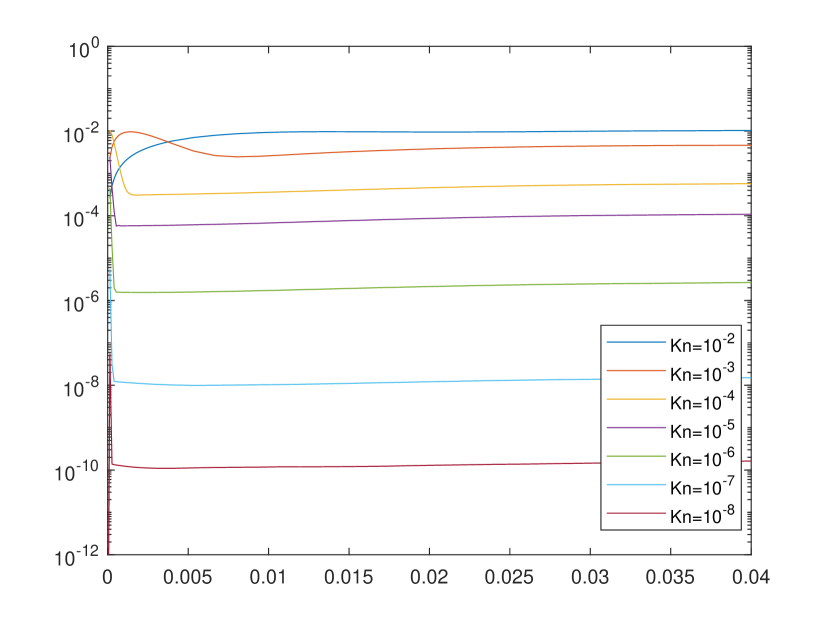
(a) AAP and BBGSP models

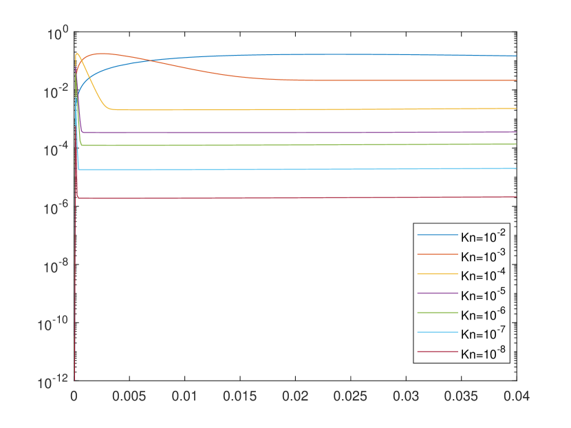
(b) AAP and GS models

Figure 1. Time evolution of relative $L^{1}$-norm of the differences in the distribution functions $g_{1}$ between BGK models for various values of $\varepsilon$.

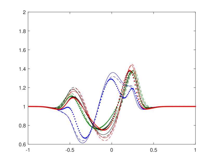
(a) Density $\rho_{s}$, $s=1,2,3,4$

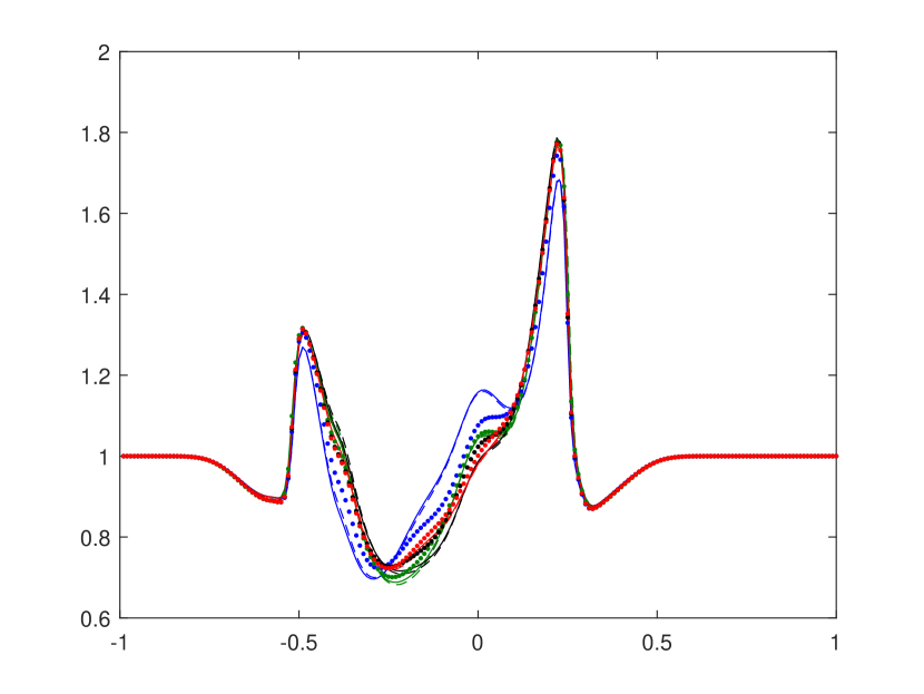
(b) Density $\rho_{s}$, $s=1,2,3,4$

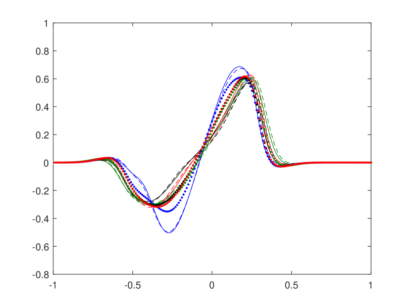
(c) Velocity $u_{s}$, $s=1,2,3,4$

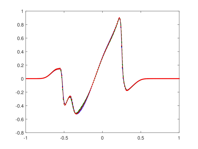
(d) Velocity $u_{s}$, $s=1,2,3,4$

(e) Temperature $T_{s}$, $s=1,2,3,4$

(f) Temperature $T_{s}$, $s=1,2,3,4$

Figure 2. Comparison of the three BGK models for $\varepsilon=10^{-2}$ (Left) and $\varepsilon=10^{-3}$ (Right) with initial data in (6.8).

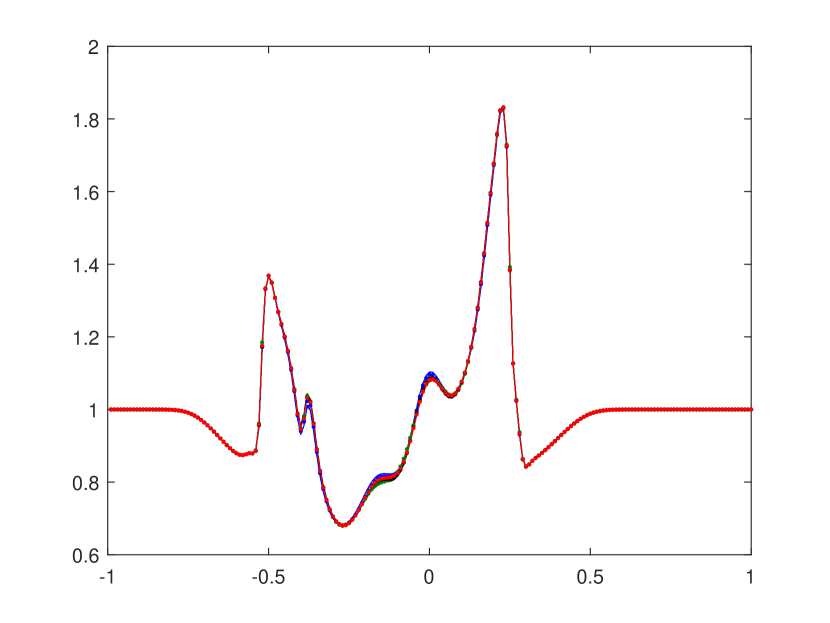
(a) Density $\rho_{s}$, $s=1,2,3,4$

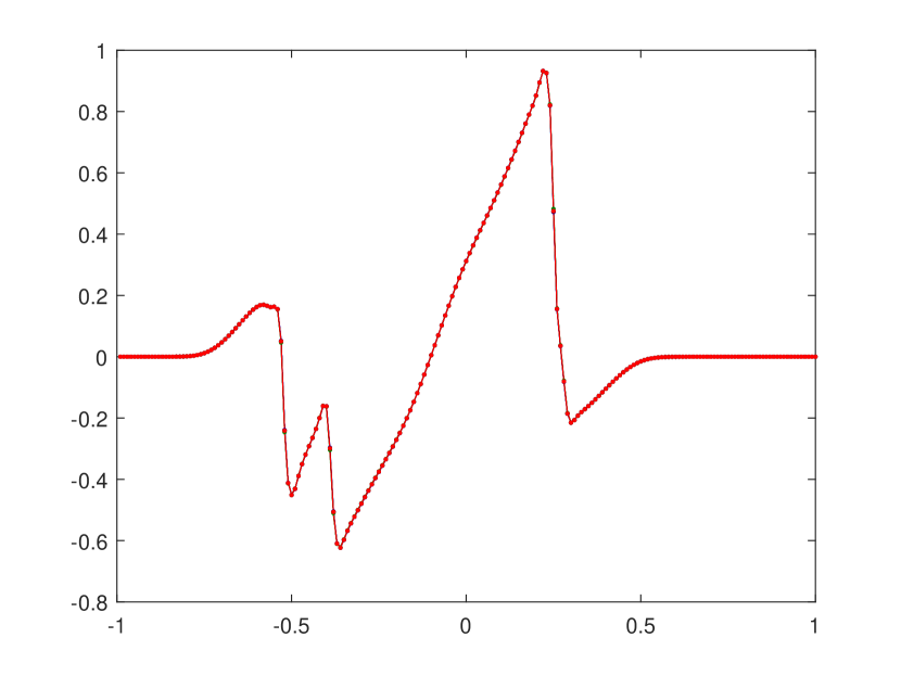
(b) Velocity $u_{s}$, $s=1,2,3,4$

Figure 3. Comparison of the three BGK models for $\varepsilon=10^{-4}$ with initial data in (6.8).

In Figs 2-3, we plotted the numerical solutions of the four gases obtained with the three BGK methods at $t_{f}=0.2$, using CFL$=0.2$ up to $t=0.02$ and CFL$=2$ for $t\in[0.02,0.2]$. The results show that some difference appears for $\varepsilon=10^{-2}$, especially between GS models and the other ones, which instead remain closer to each other, but all species velocities and temperatures are close to global velocity and temperature already from $\varepsilon=10^{-3}$, while densities equalize slower. Although we took smooth initial data, it is noticeable that shocks appear as time flows around $x=0.27$. Figure 3(a) shows even that densities are almost overlapped for $\varepsilon=10^{-4}$. Here we omit the profiles of temperature since they show similar trends of Figure 2(f).

6.2. Comparison with NS equations

Here we focus on the different hydrodynamic limits that can be obtained from the BGK model (3.7) in order to highlight their peculiar behaviors.

6.2.1. Case 1: global velocity and temperature

In this test, we check the capability to capture hydrodynamic limit (5.1) by solving model (3.7). For this, we consider the same test proposed in [1, 22]. Here we consider the mixture of four monoatomic gases with molecular masses in (6.2) and collision frequencies in (6.3).

We set initial data as Maxwellians whose macroscopic fields are

(6.9) $$\begin{split}n_{0}^{s}(x)=\frac{1}{m_{s}},\quad T_{0}^{s}(x)=\frac{4}{\sum_{s=1}^{4}n_{0}^{s}},\qquad\qquad\qquad\qquad\cr u_{0}^{s}(x)=\frac{s}{\sigma_{s}}\left[\exp\left(-\left(\sigma_{s}x-1+\frac{s}{3}\right)^{2}\right)+\exp\left(-\left(\sigma_{s}x+3-\frac{s}{10}\right)^{2}\right)\right]\end{split}$$

for $s=1,\cdots,4$, where $\sigma_{s}=(10,13,16,19)$.

To confirm the agreement between the limiting solutions to (3.7) and the solutions to NS equations (5.1), we consider various choices of Knudsen numbers $\varepsilon=10^{-k}$, $k=2,3,4$. Here we compute numerical solutions to (3.7) using $N_{x}=500$ and $N_{v}=60$. We take CFL$=0.2$ up to $t=0.02$, and CFL$=2$ in $t\in[0.02,0.2]$.

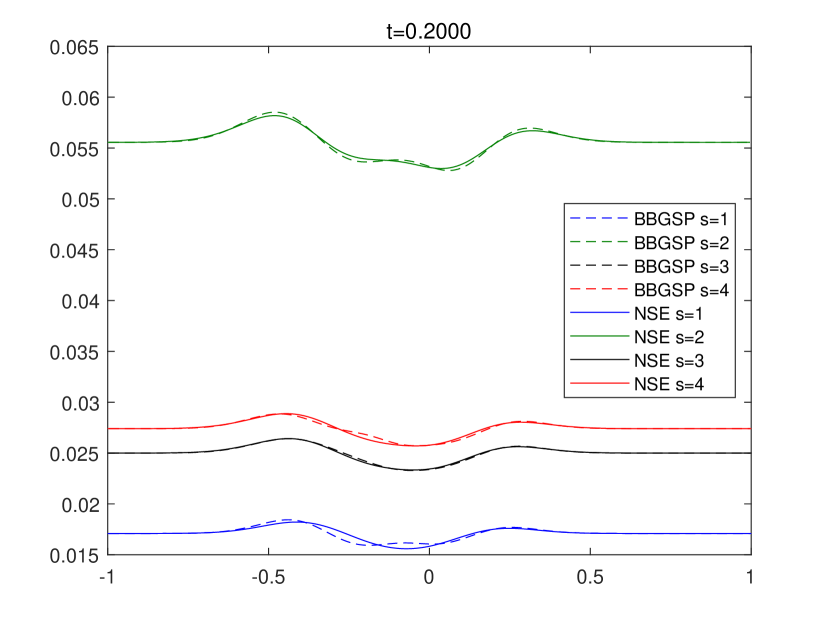
(a) Number density $n_{s}$, $s=1,2,3,4$

(b) Number density $n_{s}$, $s=1,2,3,4$

(c) Density $\rho_{s}$, $s=1,2,3,4$

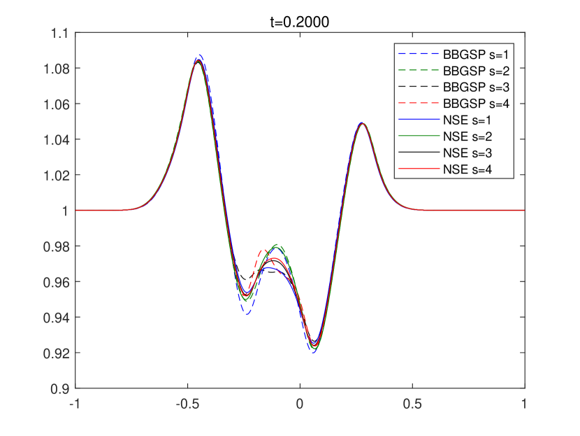
(d) Density $\rho_{s}$, $s=1,2,3,4$

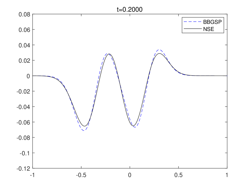
(e) Velocity $u$

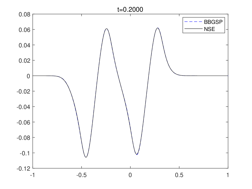
(f) Velocity $u$

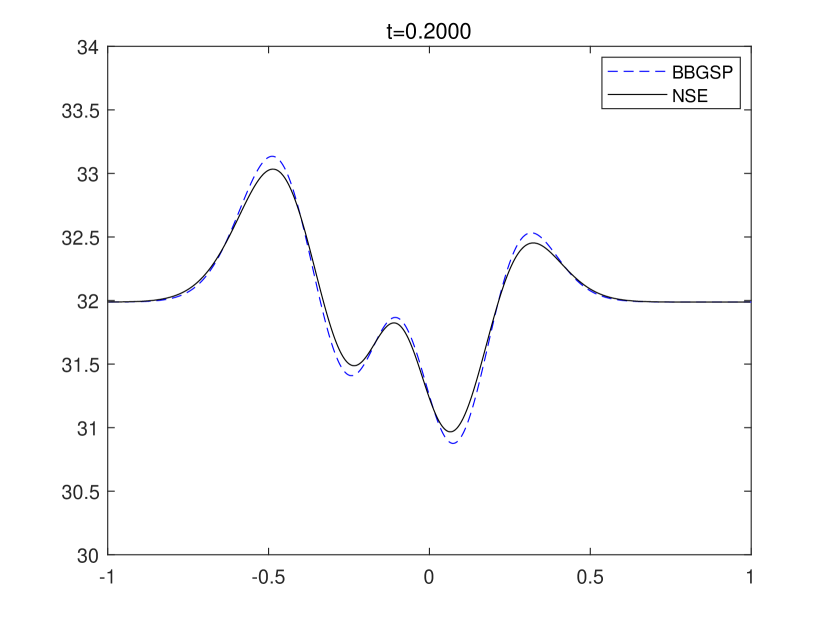
(g) Temperature $T$

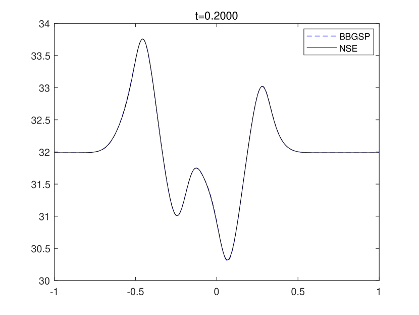
(h) Temperature $T$

Figure 4. Comparison of BGK model (3.7) and NS equations (5.1) for $\varepsilon=10^{-2}$ (Left) and $\varepsilon=10^{-3}$ (Right) with initial data in (6.9).

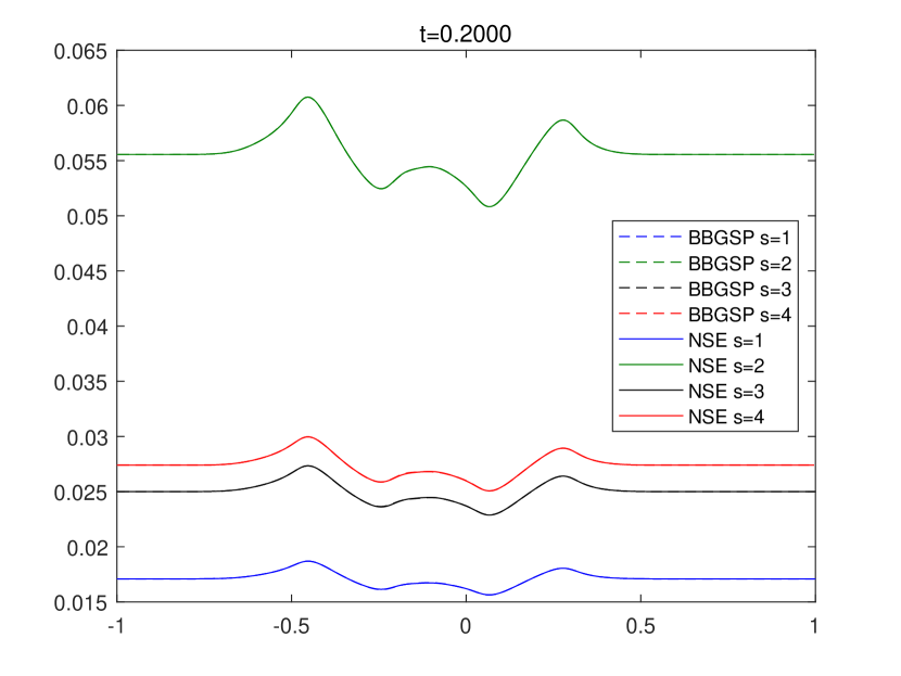
(a) Number density $n_{s}$, $s=1,2,3,4$

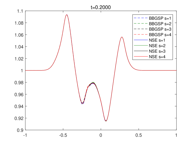
(b) Density $\rho_{s}$, $s=1,2,3,4$

(c) Velocity $u$

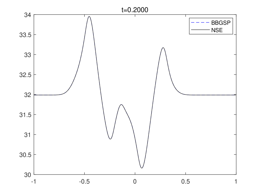
(d) Temperature $T$

Figure 5. Comparison of BGK model (3.7) and NS equations (5.1) for $\varepsilon=10^{-4}$ with initial data in (6.9).

In Figures 4, we observe that for these parameters and initial data BGK solutions (3.7) and NS solutions (5.1) are quite different for $\varepsilon=10^{-2}$. However, both solutions give similar values of macroscopic quantities as we take smaller Knudsen numbers. For $\varepsilon=10^{-3}$, global velocity $u$ and temperature $T$ are almost overlapped, contrary to species densities. In Figure 5, we note that even species densities become identical for a sufficiently small Knudsen number $\varepsilon=10^{-4}$.

6.2.2. Case 2: multi velocity and temperature

Here we consider the case in which intra-species collisions are dominant, and hence we impose $\kappa\neq\varepsilon$ in (5.9) so that the scaled version of the BBGSP model (3.7) leads to the multi-velocity and multi-temperature NS equations (5.10) for small values of $\varepsilon$. Here, we take Knudsen number $\varepsilon=10^{-k}$, $k=2,3,4$ and set $\kappa=1$. We compute numerical solutions with the same numerical setting of sect. 6.2.1.

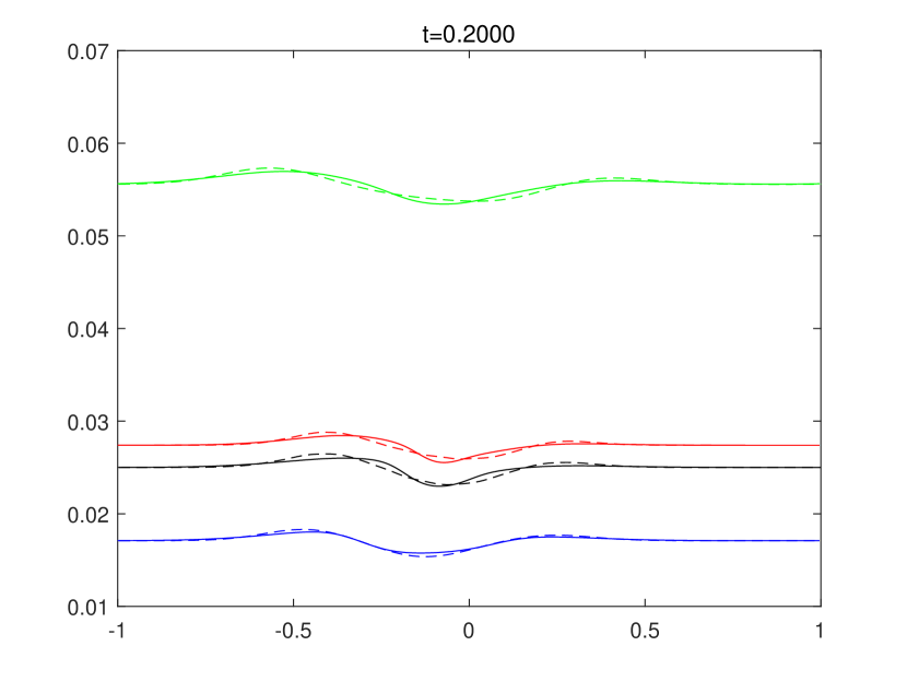
(a) Number density $n_{s}$, $s=1,2,3,4$

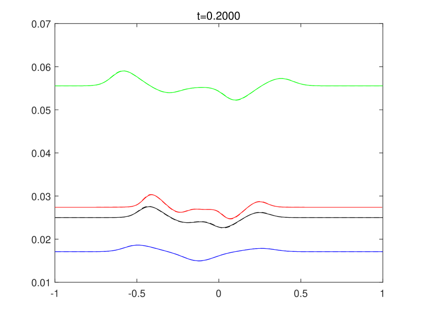
(b) Number density $n_{s}$, $s=1,2,3,4$

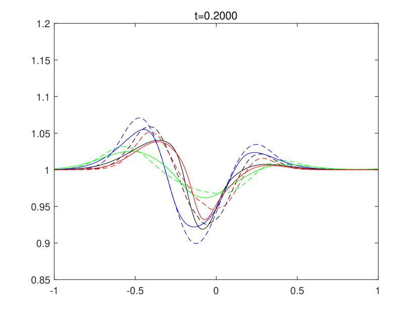
(c) Density $\rho_{s}$, $s=1,2,3,4$

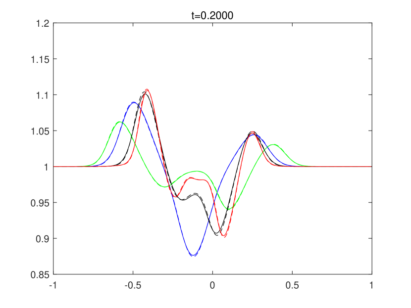
(d) Density $\rho_{s}$, $s=1,2,3,4$

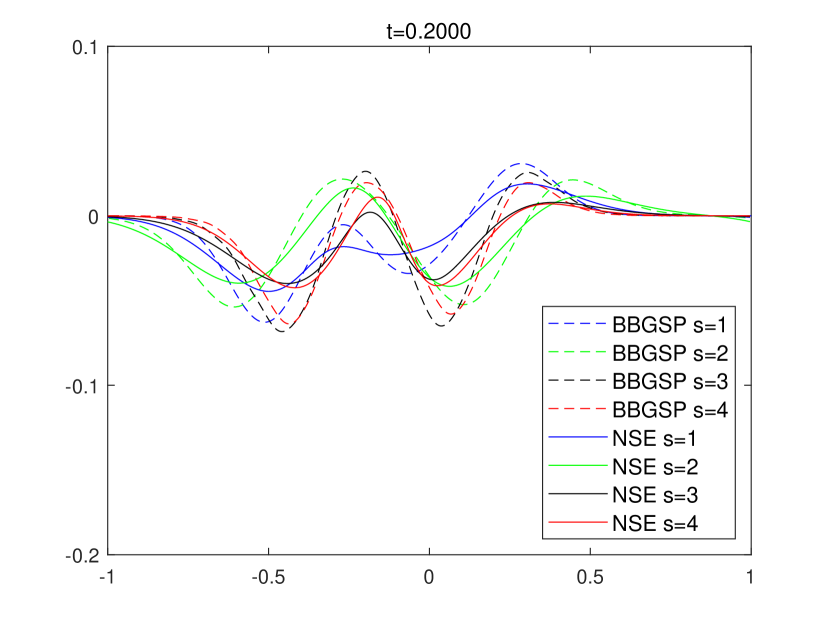
(e) Velocity $u_{s}$, $s=1,2,3,4$

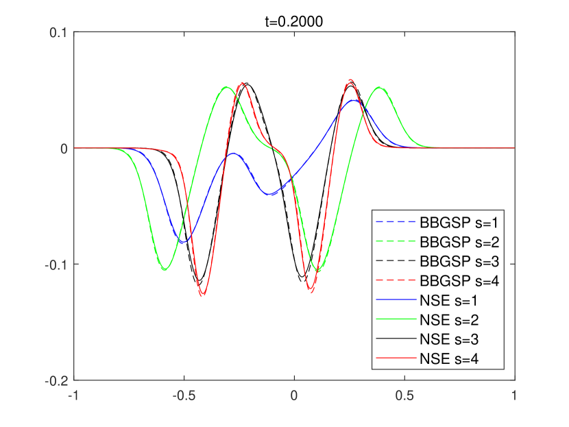
(f) Velocity $u_{s}$, $s=1,2,3,4$

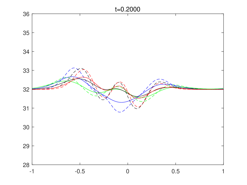
(g) Temperature $T_{s}$, $s=1,2,3,4$

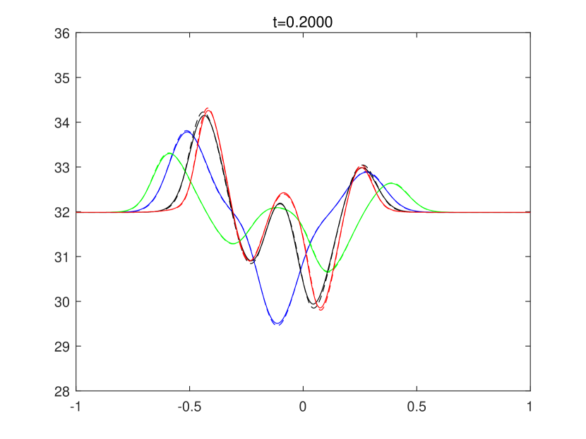
(h) Temperature $T_{s}$, $s=1,2,3,4$

Figure 6. Comparison of the scaled BBGSP model (5.9) and Navier-Stokes equations (5.10) with $\kappa=1$ for $\varepsilon=10^{-2}$ (Left) and $\varepsilon=10^{-3}$ (Right) with initial data in (6.9).

(a) Number density $n_{s}$, $s=1,2,3,4$

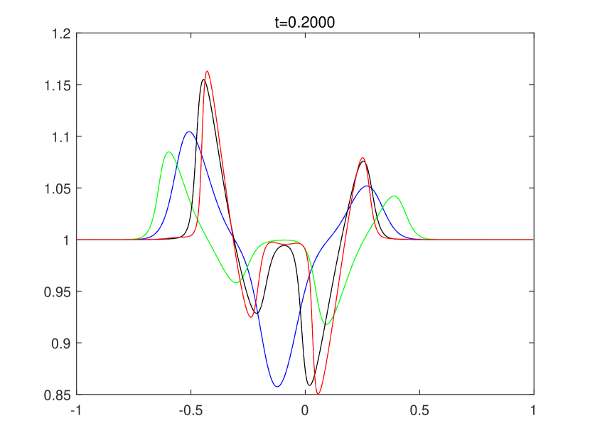
(b) Density $\rho_{s}$, $s=1,2,3,4$

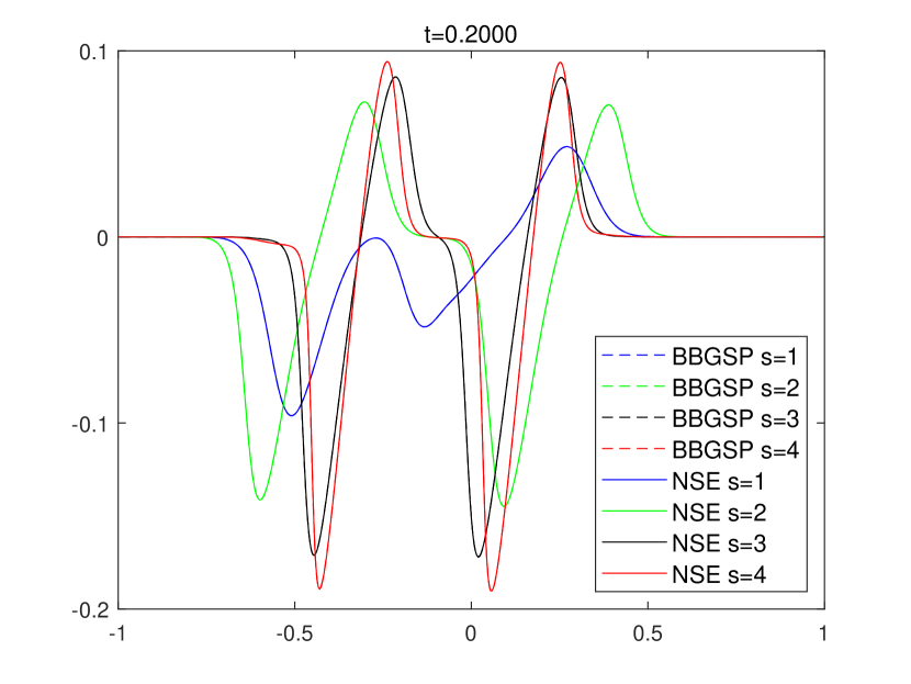
(c) Velocity $u_{s}$, $s=1,2,3,4$

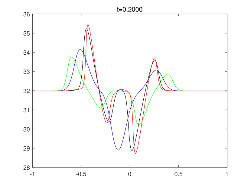
(d) Temperature $T_{s}$, $s=1,2,3,4$

Figure 7. Comparison of the scaled BBGSP model (5.9) and Navier-Stokes equations (5.10) with $\kappa=1$ for $\varepsilon=10^{-4}$ with initial data in (6.9).

In Figures 6-7, we can observe, contrary to the previous case (that can be reproduced by taking $\kappa=\varepsilon$), a clear separation between macroscopic quantities of the different species; moreover, the behavior of the BGK solutions of (5.9) are similar to those of multi-velocity and multi-temperature NS description (5.10). We note that in Figure 7 for $\varepsilon=10^{-4}$ the kinetic and macroscopic solutions show very good agreement in each species velocity and temperature.

6.3. Shock problem for binary gas mixture

In this test, we consider a shock problem for binary mixture of two noble gases: Helium (He) and Argon (Ar), for which mass ratio becomes relatively large. We aim at checking in this real case which Navier-Stokes description (for global or species macroscopic fields) is better capable to capture the behavior of the mixture.

To perform the realistic simulation, we consider molecular mass of He and Ar as follows:

$$m_{1}^{m}\approx 4\times 10^{-3}kg/mol\,(He),\quad m_{2}^{m}\approx 40\times 10^{-3}kg/mol\,(Ar).$$

In view of this, we rewrite the BBGSP model (3.7) in terms of mole. We divide $f_{s}$ by the Avogadro’s number $N_{a}\approx 6.02\times 10^{23}$. Now, we denote the molecular density by

$$f_{s}^{m}(\textbf{x},{\bf v},t):=\frac{f(\textbf{x},{\bf v},t)}{N_{a}}$$

for $s=1,2$. Then, we can rewrite (3.7) as

(6.10) $$\frac{\partial{f_{s}^{m}}}{\partial{t}}+{\bf v}\cdot\nabla_{\textbf{x}}{f_{s}^{m}}=\frac{1}{\varepsilon}\sum_{k=1}^{L}\nu_{sk}\left(n_{s}M_{sk}-f_{s}^{m}\right),\quad M_{sk}=M({\bf v};u_{sk}^{m},\frac{RT_{sk}^{m}}{m_{s}^{m}}),$$

with macroscopic quantities at the level of mole:

$$n_{s}^{m}=\langle f_{s}^{m},1\rangle,\quad n_{s}^{m}u_{s}^{m}=\langle f_{s}^{m},{\bf v}\rangle,\quad 3n_{s}^{m}RT_{s}^{m}=m_{s}^{m}\langle f_{s}^{m},|{\bf v}-u_{s}|^{2}\rangle.$$

Here we define the universal gas constant $R$ as $R:=K_{B}N_{a}\approx 8.3145\,J/mol$ and the molecular mass $m_{s}^{m}$ as $m_{s}^{m}=m_{s}N_{a}$. Note that the values of $u_{sk}^{m}$ and $T_{sk}^{m}$ are samely defined as in (3.8) by using $m_{s}^{m}$, $n_{s}^{m}$, $u_{s}^{m}$, $T_{s}^{m}$. For global macroscopic variables we use the following expressions:

$$n^{m}=\sum_{s=1}^{L}n_{s}^{m},\quad\rho^{m}=\sum_{s=1}^{L}\rho_{s}^{m},\quad\rho_{s}^{m}=m_{s}^{m}n_{s}^{m},\quad s=1,\cdots,L$$

$$u^{m}=\frac{1}{\rho^{m}}\sum_{s=1}^{L}\rho_{s}^{m}u_{s}^{m},\quad 3n^{m}RT^{m}=3\sum_{s=1}^{L}n_{s}^{m}RT_{s}^{m}+\sum_{s=1}^{L}\rho_{s}^{m}|u_{s}^{m}-u^{m}|^{2}$$

Let us consider room temperature $T_{s}^{m}=300K$. As in [5], here we use the collision frequencies corresponding to $T_{s}^{m}=300K$ based on the following formula:

(6.11) $$\begin{split}\nu_{0}^{ss}&=\frac{4}{3}\frac{T}{\mu_{s}(T)},\quad s=1,2\cr\nu_{0}^{12}&=\frac{2\sqrt{2}}{3}\frac{(m_{1}+m_{2})^{\frac{1}{4}}}{(m_{1}m_{2})^{\frac{1}{2}}}\frac{T}{(\mu_{1}(T)\mu_{2}(T))^{\frac{1}{2}}},\end{split}$$

where viscosity coefficients $\mu_{s}$ for noble gases are provided in [25]. In case of Helium and Argon, we have

$$\nu_{0}^{11}=19.96,\quad\nu_{0}^{12}=1.153$$

$$\nu_{0}^{21}=1.153,\quad\nu_{0}^{22}=17.52.$$

Note that we set $\nu_{sk}=\nu_{0}^{sk}n_{k}$. Now, we consider a shock problem by taking the Maxwellian as initial data which reproduces the following macroscopic variables:

$$\left(\rho_{0}^{m},u_{0}^{m},T_{0}^{m}\right)=\begin{cases}\left(1.7628,\,0,\,300\right),\quad x<0.5\\ \left(0.8814,\,0,\,300\right),\quad x>0.5\end{cases}$$

The units of $\rho_{0}^{m}$, $u_{0}^{m}$, $T_{0}^{m}$ are $kg/m^{3}$, $m/s$, $K$, respectively. Now, we set

$$\begin{split}\left(\rho_{01}^{m},\rho_{02}^{m}\right)&=\begin{cases}\left(0.1598,\,1.6030\right),\quad x<0.5\\ \left(0.0799,\,0.8015\right),\quad x>0.5\\ \end{cases}.\end{split}$$

Note that the density of Helium and Argon gases for $T_{0}^{m}=300K$ for $p^{m}=1\,bar$ are given by

$$\rho_{1}^{m}=0.1598\,kg/m^{3},\quad\rho_{2}^{m}=1.603\,kg/m^{3}.$$

For numerical simulation, we assume the free-flow boundary condition on the spatial domain $x\in[-6,6]$ with velocity domain $v\in[-160,160]$. We compute numerical solutions with $N_{x}=600$ and $N_{v}=320$ up to $t_{f}=0.06$. Here we use CFL=$1.5$ and take different values of $\varepsilon=10^{-q}$, $q=3,4,5$.

In Figure 8, for relatively large values of $\kappa=10^{-3}$, the panels on the left column show that the global velocity and temperature is closely related to the dynamics of Argon gas. This is because its density is ten times bigger than that of Helium gas. Thus, it is difficult to describe the dynamics of mixtures involving Helium gas with global velocity and temperature description. On the other hand, the panels on the right column enables us to capture the behaviors of Helium gas and this is the case where multi-velocity and multi-temperature description can be a suitable model for a better description of this dynamics. In the following Figures 9-10, both species velocities and temperatures are close to global velocity and temperature. Here the global velocity and temperature Euler system can be already a suitable choice for describing the dynamics of binary mixtures.

In the right panels of Figures 8-10, we observe that the species velocity and temperature for light gas show very different behaviors as both $\varepsilon$ and $\kappa$ becomes smaller. For a better understanding of these observations with the scaled BBGSP model (5.9), let us consider binary gas mixtures with $m_{2}=rm_{1}$ where $r<1$ denotes their mass ratio. Then, in the limit $r\rightarrow 0$, we obtain

$$M_{12} \rightarrow M\left({\bf v};u_{1},\frac{K_{B}T_{1}}{m_{1}}\right),\quad M_{21}\rightarrow M\left({\bf v};u_{1},\frac{K_{B}T_{2}}{m_{2}}+\frac{1}{3}|u_{1}-u_{2}|^{2}\right),$$

while $M_{ss}=M\left(v;u_{s},\frac{K_{B}T_{s}}{m_{s}}\right)$ for $s=1,2$. The form of $M_{12}$ and $M_{21}$ implies that as the intra-species collisions becomes dominant, light gas tends to follow the behavior of heavy gas:

$$\frac{\partial{f_{2}}}{\partial{t}}+{\bf v}\cdot\nabla_{\textbf{x}}{f_{2}} =\frac{\nu_{21}}{\kappa}\left(n_{2}M\left({\bf v};u_{1},\frac{K_{B}T_{2}}{m_{2}}+\frac{1}{3}|u_{1}-u_{2}|^{2}\right)-f_{2}\right)+\frac{\nu_{22}}{\varepsilon}\left(n_{2}M_{22}-f_{2}\right),$$

while heavy gas tends to behave like a single gas:

$$\frac{\partial{f_{1}}}{\partial{t}}+{\bf v}\cdot\nabla_{\textbf{x}}{f_{1}} =\frac{\nu_{11}}{\varepsilon}\left(n_{1}M_{11}-f_{1}\right)+\frac{\nu_{12}}{\kappa}\left(n_{1}M\left({\bf v};u_{1},\frac{K_{B}T_{1}}{m_{1}}\right)-f_{1}\right).$$

Furthermore, the formula (6.11) for noble gases gives

$$\nu_{0}^{12} =\frac{2\sqrt{2}}{3}\left(\frac{m_{2}}{m_{1}}\right)^{\frac{1}{4}}\frac{\left(1+\frac{m_{2}}{m_{1}}\right)^{\frac{1}{4}}}{(m_{2})^{\frac{1}{2}}}\frac{T}{(\mu_{1}(T)\mu_{2}(T))^{\frac{1}{2}}}=\frac{2\sqrt{2}}{3}r^{\frac{1}{4}}\frac{(1+r)^{\frac{1}{4}}}{(m_{2})^{\frac{1}{2}}}\frac{T}{\left(\mu_{1}(T)\mu_{2}(T)\right)^{\frac{1}{2}}},$$

in which, for a fixed value of $m_{2}>0$ the limit $r\rightarrow 0$ implies $\nu_{0}^{12}\rightarrow 0$. If $\nu_{0}^{12}<<\kappa$, the scaled BBGSP model (5.9) formally reduces to two independent equations:

$$\frac{\partial{f_{1}}}{\partial{t}}+{\bf v}\cdot\nabla_{\textbf{x}}{f_{1}} =\frac{\nu_{11}}{\varepsilon}\left(n_{1}M\left({\bf v};u_{1},\frac{K_{B}T_{1}}{m_{1}}\right)-f_{1}\right)$$

$$\frac{\partial{f_{2}}}{\partial{t}}+{\bf v}\cdot\nabla_{\textbf{x}}{f_{s}} =\frac{\nu_{22}}{\varepsilon}\left(n_{2}M\left({\bf v};u_{2},\frac{K_{B}T_{2}}{m_{2}}\right)-f_{2}\right).$$

where $\nu_{ss}=\nu_{0}^{ss}n_{s}$.

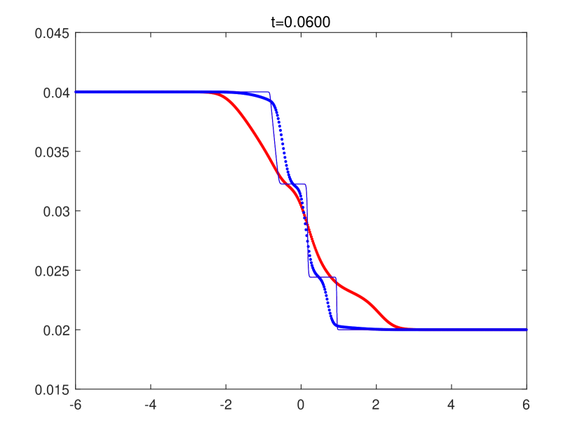
(a) Number density $n_{s}$, $s=1,2$

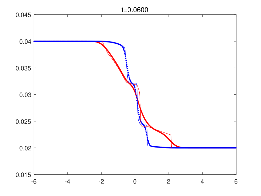
(b) Number density $n_{s}$, $s=1,2$

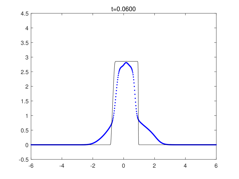
(c) Velocity $u$

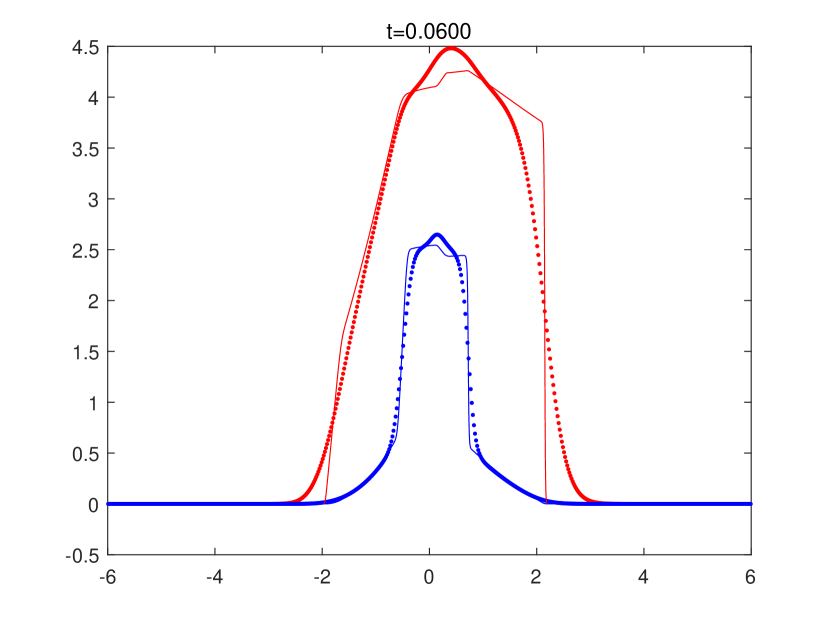
(d) Velocity $u$

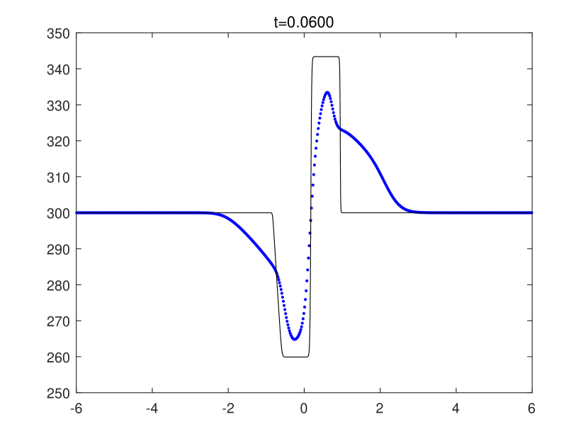
(e) Temperature $T$

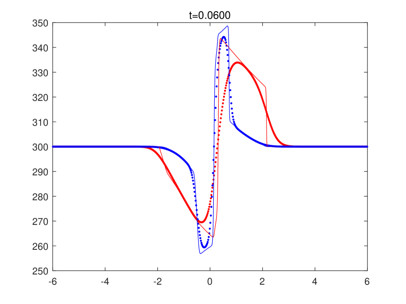
(f) Temperature $T$

Figure 8. Comparison of the scaled BBGSP model (5.9) for $\varepsilon=\kappa=10^{-3}$ with: (left) global velocity and temperature Euler system (5.1) for $\varepsilon=0$ and (right) multi-velocity and multi-temperature Euler system (5.10) for $\varepsilon=0$, $\kappa=10^{-3}$. We use the initial data in (6.3).

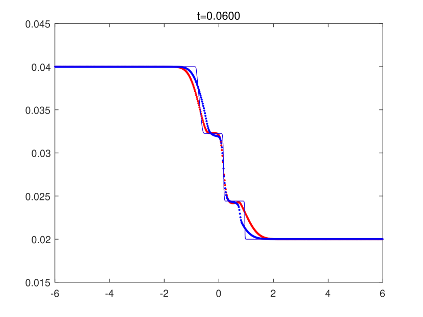
(a) Number density $n_{s}$, $s=1,2$

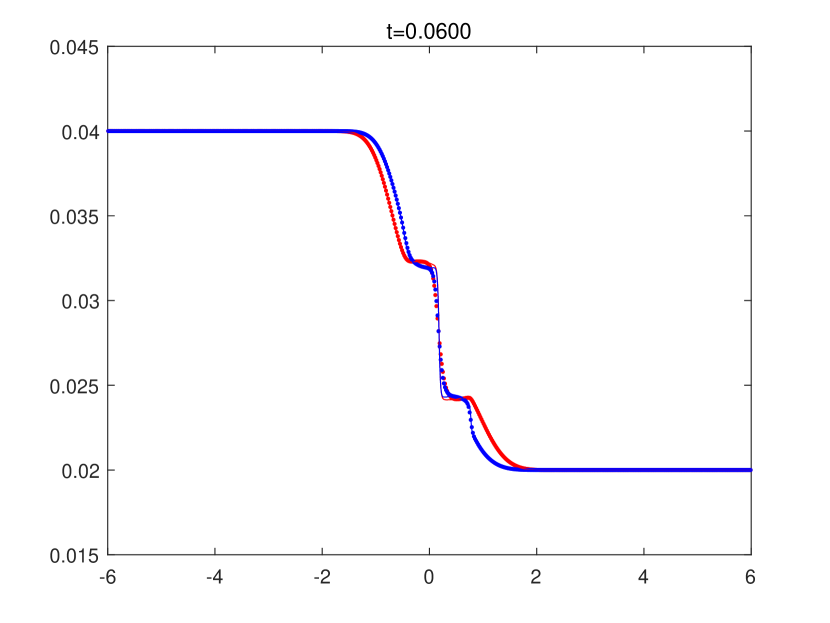
(b) Number density $n_{s}$, $s=1,2$

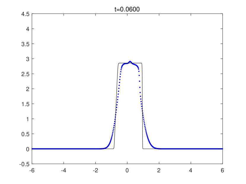
(c) Velocity $u$

(d) Velocity $u$

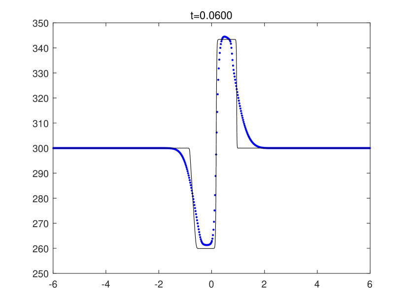
(e) Temperature $T$

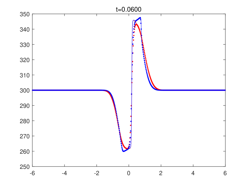
(f) Temperature $T$

Figure 9. Comparison of the scaled BBGSP model (5.9) for $\varepsilon=\kappa=10^{-4}$ with: (left) global velocity and temperature Euler system (5.1) for $\varepsilon=0$ and (right) multi-velocity and multi-temperature Euler system (5.10) for $\varepsilon=0$, $\kappa=10^{-4}$. We use the initial data in (6.3).

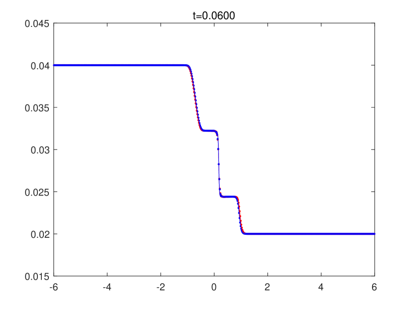
(a) Number density $n_{s}$, $s=1,2$

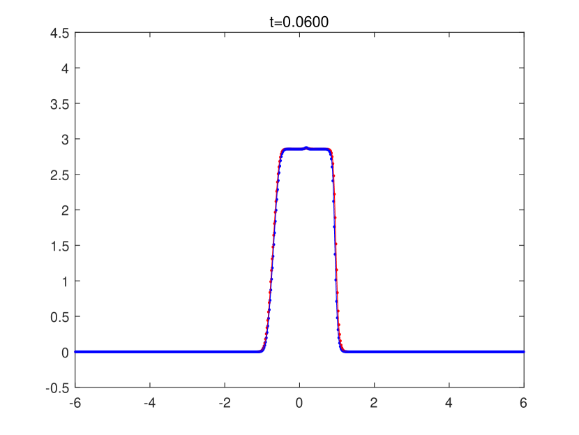
(b) Velocity $u$

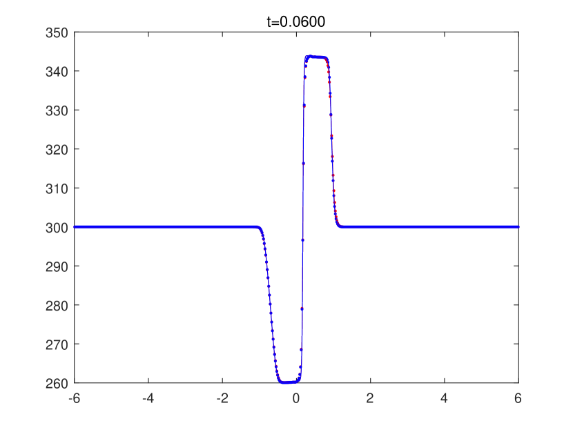
(c) Temperature $T$

Figure 10. Comparison of the scaled BBGSP model (5.9) for $\varepsilon=\kappa=10^{-5}$ with multi-velocity and multi-temperature Euler system (5.10) for $\varepsilon=0$, $\kappa=10^{-5}$. We use the initial data in (6.3).

6.4. Stationary shock

In this test, we consider a classical problem of gas dynamics, namely the shock wave structure obtained by the Navier-Stokes description in a binary mixture of two noble gases: Neon (Ne) and Argon (Ar). This problem has been faced in [5] by using the qualitative theory of dynamical systems applied to the time-independent version of the NS equations, which can be rewritten as a suitable system of first order ODEs. Here we alternatively obtain the stationary shock solution as asymptotic solution of the time-dependent Navier-Stokes equations (5.1) and also by solving the BBGSP model.

For this test, we consider molecular masses:

$$m_{1}=20\text{(Ne)},\quad m_{2}=40\text{(Ar)}.$$

Based on (6.11), we set collision frequencies for $T=300$K by

$$\nu_{0}^{11}=12.46,\quad\nu_{0}^{12}=15.22$$

$$\nu_{0}^{21}=15.22,\quad\nu_{0}^{22}=17.52.$$

We take initial data by the Maxwellian whose macroscopic fields reproduce

$$\begin{split}\begin{pmatrix}n_{s}(x,0)\\ u_{s}(x,0)\\ T_{s}(x,0)\end{pmatrix}=E_{L}^{s}+\frac{E_{R}^{s}-E_{L}^{s}}{2}\big{(}\tanh(ax)+1\big{)},\quad x\in[-20,20]\end{split}$$

where $a$ is a parameter which adjusts the slope of the smooth jump associated to the initial data (we take $a=2$). The two states $E_{L}^{s}$ and $E_{R}^{s}$, $s=1,2$, are chosen according to the Rankine-Hugoniot conditions as follows [5]:

$$\begin{split}E_{R}^{s}&=\left(n_{s}^{\infty},u^{\infty},T^{\infty}\right),\\ E_{L}^{s}&=\left(\frac{4M\!a^{2}}{M\!a^{2}+3}n_{s}^{\infty},\,\frac{M\!a^{2}+3}{4M\!a^{2}}u^{\infty},\,\frac{(5M\!a^{2}-1)(M\!a^{2}+3)}{16M\!a^{2}}T^{\infty}\right)\cr c^{\infty}&=\sqrt{\frac{5n^{\infty}T^{\infty}}{3\rho^{\infty}}}=\sqrt{\frac{5(n_{1}^{\infty}+n_{2}^{\infty})T^{\infty}}{3(\rho_{1}^{\infty}+\rho_{2}^{\infty})}}\cr M\!a&=\sqrt{\frac{u^{\infty}}{c^{\infty}}},\end{split}$$

where $M\!a$ is the Mach number. We consider concentrations $\displaystyle\chi_{1}=\frac{n_{1}}{n}=0.1$ and $\displaystyle\chi_{2}=\frac{n_{2}}{n}=0.9$, and set

$$n_{1}=\chi_{1}n,\quad n_{2}=\chi_{2}n,\quad M\!a=\sqrt{0.6},\quad T^{\infty}=300.$$

In this problem, we impose the inflow and outflow boundary conditions. We consider velocity domain $[-32,32]$ and compute numerical solutions with $N_{v}=80$, $N_{x}=200$ and CFL$=0.5$. For comparison, we set $\varepsilon=1$ for this problem.

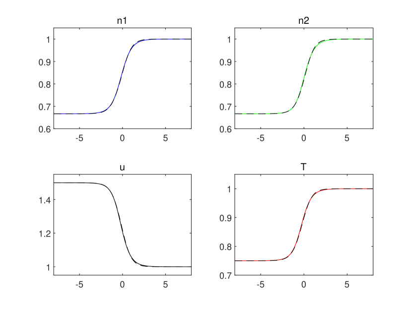
Figure 11. BDF3-QCWENO35 for $\varepsilon=\kappa=10^{-0}$. Neon and Argon with $n_{1}=0.1m_{1},\quad n_{2}=0.9m_{2}$. Black dashed lines are reference NS solutions and solid lines are BGK solutions.

In Figure 11, we plot normalized macroscopic fields:

$$n_{s}/n_{s}^{\infty},\quad u/u^{\infty},\quad T/T^{\infty}.$$

Our solution shows very good agreement between the long-time solution of the BBGSP model and the reference solution asymptotically obtained from the NS equations (5.1) discretized by a MacCormack scheme $(N_{x}=800)$. Moreover, the results are in accordance with the steady shock wave solution that can be obtained by solving the stationary (ODEs) system of Navier-Stokes equations [5]. For other relevant tests, we refer to [5].

Appendix A Leading error terms in Proposition 4.1 and Remark 4.1

A.1. Proof of Proposition 4.1

Proof.

$\bullet$ Proof of (1): To show this, we first express $u^{s}$ and $u_{sk}$ in terms of $u_{s}$ and $u_{k}$ in $\mathcal{E}_{u}$:

$$\sum_{k=1}^{L}\nu_{sk}(u^{s}-u_{sk}) =\sum_{k=1}^{L}\nu_{sk}\bigg{[}\left(u_{s}+\frac{1}{m_{s}n_{s}\nu_{s}}\sum_{r=1}^{L}\xi^{sr}u_{r}\right)-\left((1-a_{sk})u_{s}+a_{sk}u_{k}\right)\bigg{]}$$

$$=\sum_{k=1}^{L}\nu_{sk}\bigg{[}\left(\frac{1}{m_{s}n_{s}\nu_{s}}\sum_{r=1}^{L}\xi^{sr}u_{r}\right)-a_{sk}(u_{k}-u_{s})\bigg{]}.$$

By the definition of $\xi^{sr}$ in (3.3) and $a_{sk}$ in (3.9), we obtain

$$\sum_{k=1}^{L}\nu_{sk}(u^{s}-u_{sk}) =\sum_{k=1}^{L}\nu_{sk}\bigg{[}\left(\frac{1}{m_{s}n_{s}\nu_{s}}\sum_{r=1}^{L}\xi^{sr}u_{r}\right)-a_{sk}(u_{k}-u_{s})\bigg{]}$$

$$=\sum_{r=1}^{L}\left(\frac{\nu_{1}^{sr}m_{r}n_{r}}{m_{s}+m_{r}}-\delta_{sr}\sum_{\ell=1}^{L}\frac{\nu_{1}^{s\ell}m_{\ell}n_{\ell}}{m_{s}+m_{\ell}}\right)u_{r}-\sum_{k=1}^{L}\bigg{[}\frac{\lambda_{sk}m_{k}n_{k}}{m_{s}+m_{k}}(u_{k}-u_{s})\bigg{]}=0.$$

In the last line, we use the relation $\nu_{1}^{s\ell}=\lambda_{s\ell}$ in (3.4).
Proof (2): To prove this, we begin by splitting in $\mathcal{E}_{T}$ (4.1) into two parts:

$$\sum_{k=1}^{L}\nu_{sk}(T^{s}-T_{sk}) =I+II+III,$$

where

$$I =\sum_{k=1}^{L}\nu_{sk}\bigg{[}\frac{2}{3n_{s}K_{B}\nu_{s}}\sum_{r=1}^{L}\gamma^{sr}T_{r}-b_{sk}(T_{k}-T_{s})\bigg{]}$$

$$II =\frac{2m_{s}}{3K_{B}}\sum_{r=1}^{L}\nu_{sr}\bigg{[}\nu_{1}^{sr}\frac{m_{r}n_{r}}{\nu_{sr}(m_{s}+m_{r})^{2}}\left(m_{s}u_{s}+m_{r}u_{r}\right)\left(u_{r}-u_{s}\right)\bigg{]}-\sum_{k=1}^{L}\nu_{sk}\frac{\gamma_{sk}}{K_{B}}|u_{s}-u_{k}|^{2}$$

$$III =-\frac{m_{s}}{3K_{B}}\sum_{k=1}^{L}\nu_{sk}\bigg{[}|u^{s}|^{2}-|u_{s}|^{2}\bigg{]}$$

Inserting $\gamma^{sr}$ in (3.3) into $I$, we have

$$I =\frac{2}{3n_{s}K_{B}}\sum_{r=1}^{L}\gamma^{sr}T_{r}-\sum_{k=1}^{L}\nu_{sk}b_{sk}(T_{k}-T_{s})$$

$$=2\sum_{r=1}^{L}\left(\nu_{1}^{sr}\frac{m_{s}m_{r}n_{r}}{(m_{s}+m_{r})^{2}}-\delta_{sr}\sum_{\ell=1}^{L}\nu_{1}^{s\ell}\frac{m_{s}m_{\ell}n_{\ell}}{(m_{s}+m_{\ell})^{2}}\right)T_{r}-\sum_{k=1}^{L}\nu_{sk}b_{sk}(T_{k}-T_{s})$$

$$=0.$$

In the last line, we use $\displaystyle b_{sk}=\frac{2a_{sk}m_{s}}{m_{s}+m_{k}}=\frac{2\lambda_{sk}m_{s}m_{k}n_{k}}{\nu_{sk}(m_{s}+m_{r})^{2}}$ and $\nu_{1}^{sk}=\lambda_{sk}.$ Next, we simplify $II$ as

$$II =\frac{2m_{s}}{3K_{B}}\sum_{r=1}^{L}\nu_{sr}\bigg{[}a_{sr}\left(u_{s}+\frac{m_{r}}{m_{s}+m_{r}}(u_{r}-u_{s})\right)\cdot\left(u_{r}-u_{s}\right)\bigg{]}-\sum_{k=1}^{L}\nu_{sk}\frac{\gamma_{sk}}{K_{B}}|u_{s}-u_{k}|^{2}$$

$$=\frac{2m_{s}}{3K_{B}}\sum_{r=1}^{L}\nu_{sr}\bigg{[}a_{sr}u_{s}\cdot\left(u_{r}-u_{s}\right)+a_{sr}\frac{m_{r}}{m_{s}+m_{r}}|u_{r}-u_{s}|^{2}\bigg{]}-\sum_{k=1}^{L}\nu_{sk}\frac{\gamma_{sk}}{K_{B}}|u_{s}-u_{k}|^{2}$$

This combined with $\gamma_{sk}$ in (3.9) gives

$$II =\frac{2m_{s}}{3K_{B}}\sum_{r=1}^{L}\nu_{sk}a_{sk}\bigg{[}u_{s}\cdot\left(u_{k}-u_{s}\right)\bigg{]}+\frac{m_{s}}{3K_{B}}\sum_{k=1}^{L}\nu_{sk}(a_{sk})^{2}|u_{s}-u_{k}|^{2}.$$

Now, the following relation

$$|u_{sk}|^{2}=|a_{sk}(u_{s}-u_{k})-u_{s}|^{2}=(a_{sk})^{2}|u_{s}-u_{k}|^{2}-2a_{sk}(u_{s}-u_{k})\cdot u_{s}+|u_{s}|^{2}$$

implies

$$II+III =-\frac{m_{s}}{3K_{B}}\sum_{k=1}^{L}\nu_{sk}\bigg{[}|u^{s}|^{2}-|u_{sk}|^{2}\bigg{]}.$$

To simplify further this, recall the relation

(A.1) $$u^{s} =u_{s}+\frac{1}{\nu_{s}}\sum_{r=1}^{L}\nu_{sr}a_{sr}(u_{r}-u_{s}),$$

and use this to get

$$II+III =-\frac{m_{s}}{3K_{B}}\sum_{k=1}^{L}\nu_{sk}\left[2u_{s}+\frac{1}{\nu_{s}}\sum_{r=1}^{L}\nu_{sr}a_{sr}(u_{r}-u_{s})-a_{sk}(u_{s}-u_{k})\right]$$

$$\qquad\qquad\qquad\cdot\left[\frac{1}{\nu_{s}}\sum_{r=1}^{L}\nu_{sr}a_{sr}(u_{r}-u_{s})+a_{sk}(u_{s}-u_{k})\right]$$

$$=A+B$$

where

$$A =-\frac{m_{s}}{3K_{B}}\sum_{k=1}^{L}\nu_{sk}\left[2u_{s}+\frac{1}{\nu_{s}}\sum_{r=1}^{L}\nu_{sr}a_{sr}(u_{r}-u_{s})\right]\left[\frac{1}{\nu_{s}}\sum_{r=1}^{L}\nu_{sr}a_{sr}(u_{r}-u_{s})\right]$$

$$=-\frac{m_{s}}{3\nu_{s}K_{B}}\left[2u_{s}\nu_{s}+\sum_{r=1}^{L}\nu_{sr}a_{sr}(u_{r}-u_{s})\right]\cdot\left[\sum_{r=1}^{L}\nu_{sr}a_{sr}(u_{r}-u_{s})\right]$$

$$B =-\left(\frac{2m_{s}u_{s}}{3K_{B}}\cdot\sum_{k=1}^{L}\nu_{sk}a_{sk}(u_{s}-u_{k})-\frac{m_{s}}{3K_{B}}\sum_{k=1}^{L}\nu_{sk}(a_{sk})^{2}|u_{s}-u_{k}|^{2}\right).$$

To be more concise, we can rewrite $A$ and $B$ as

$$A =-\frac{2m_{s}u_{s}}{3K_{B}}\cdot X-\frac{m_{s}}{3\nu_{s}K_{B}}|X|^{2}$$

$$B =\frac{2m_{s}u_{s}}{3K_{B}}\cdot X+\frac{m_{s}}{3K_{B}}Y$$

where

$$X=\sum_{r=1}^{L}\nu_{sr}a_{sr}(u_{r}-u_{s}),\quad Y=\sum_{r=1}^{L}\nu_{sr}(a_{sr})^{2}|u_{r}-u_{s})|^{2}.$$

Then, we have

$$II+III$$

$$=\frac{m_{s}}{3K_{B}}\sum_{k=1}^{L}\nu_{sk}(a_{sk})^{2}|u_{s}-u_{k}|^{2}-\frac{m_{s}}{3\nu_{s}K_{B}}\left(\sum_{r=1}^{L}\nu_{sr}a_{sr}(u_{r}-u_{s})\right)\cdot\left(\sum_{r=1}^{L}\nu_{sr}a_{sr}(u_{r}-u_{s})\right),$$

which gives the desired result. ∎

A.2. Calculation of $\bar{\mathcal{E}}_{u}$ and $\bar{\mathcal{E}}_{T}$ terms in (4.2).

Proof.

$\bullet$ Proof of (1): We first rewrite $\bar{u}$ as

$$\bar{u} =u_{s}+\frac{1}{\sum_{r=1}^{L}\nu_{r}m_{r}n_{r}}\sum_{r\neq s}\nu_{r}m_{r}n_{r}(u_{r}-u_{s}).$$

This, combined with the expression of $u^{s}$ in (A.1), gives

$$\bar{\mathcal{E}}_{u} =\nu_{s}(u^{s}-\bar{u})$$

$$=\nu_{s}\left(\frac{1}{\nu_{s}}\sum_{r\neq s}\left(\nu_{1}^{sr}\frac{m_{r}n_{r}}{m_{s}+m_{r}}\right)(u_{r}-u_{s})-\frac{1}{\sum_{r=1}^{L}\nu_{r}m_{r}n_{r}}\sum_{r\neq s}\nu_{r}m_{r}n_{r}(u_{r}-u_{s})\right)$$

$$=\sum_{r\neq s}\left(\nu_{1}^{sr}\frac{m_{r}n_{r}}{m_{s}+m_{r}}-\frac{\nu_{s}\nu_{r}m_{r}n_{r}}{\sum_{r=1}^{L}\nu_{r}m_{r}n_{r}}\right)(u_{r}-u_{s}).$$

Proof (2):

From the definition of $T^{s}$ and $\bar{T}$, we have

$$\bar{\mathcal{E}}_{T} =\nu_{s}(T^{s}-\bar{T})$$

$$=\nu_{s}\bigg{[}T_{s}-\frac{m_{s}}{3K_{B}}\left(|u^{s}|^{2}-|u_{s}|^{2}\right)+\frac{2}{3n_{s}K_{B}\nu_{s}}\sum_{r=1}^{L}\gamma^{sr}T_{r}$$

$$\qquad\qquad+\frac{2}{3n_{s}K_{B}\nu_{s}}\sum_{r=1}^{L}\nu_{1}^{sr}\frac{m_{s}m_{r}n_{s}n_{r}}{(m_{s}+m_{r})^{2}}\left(m_{s}u_{s}+m_{r}u_{r}\right)\left(u_{r}-u_{s}\right)$$

$$\qquad\qquad-\left(T_{s}-\frac{\sum_{r=1}^{L}\nu_{r}n_{r}m_{r}\left(|\bar{u}|^{2}-|u_{r}|^{2}\right)}{3K_{B}\sum_{r=1}^{L}\nu_{r}n_{r}}+\frac{\sum_{r\neq s}\nu_{r}n_{r}(T_{r}-T_{s})}{\sum_{r=1}^{L}\nu_{r}n_{r}}\right)\bigg{]}$$

$$=J_{1}+J_{2}+J_{3},$$

where

$$J_{1} =\nu_{s}\left[T_{s}+\frac{2}{3n_{s}K_{B}\nu_{s}}\sum_{r=1}^{L}\gamma^{sr}T_{r}-\left(T_{s}-\frac{\sum_{r=1}^{L}\nu_{r}n_{r}m_{r}\left(|\bar{u}|^{2}-|u_{r}|^{2}\right)}{3K_{B}\sum_{r=1}^{L}\nu_{r}n_{r}}+\frac{\sum_{r\neq s}\nu_{r}n_{r}(T_{r}-T_{s})}{\sum_{r=1}^{L}\nu_{r}n_{r}}\right)\right]$$

$$J_{2} =\nu_{s}\left[\frac{\sum_{r=1}^{L}\nu_{r}n_{r}m_{r}\left(|\bar{u}|^{2}-|u_{r}|^{2}\right)}{3K_{B}\sum_{r=1}^{L}\nu_{r}n_{r}}\right]$$

$$J_{3} =\sum_{k=1}^{L}\nu_{sk}\bigg{[}-\frac{m_{s}}{3K_{B}}\left(|u^{s}|^{2}-|u_{s}|^{2}\right)+\frac{2}{3K_{B}\nu_{s}}\sum_{r=1}^{L}\nu_{1}^{sr}\frac{m_{s}m_{r}n_{r}}{(m_{s}+m_{r})^{2}}\left(m_{s}u_{s}+m_{r}u_{r}\right)\left(u_{r}-u_{s}\right)\bigg{]}.$$

For $J_{1}$, we use

$$\gamma^{sr}=3K_{B}\nu_{1}^{sr}\frac{m_{s}m_{r}n_{s}n_{r}}{(m_{s}+m_{r})^{2}}-\delta_{sr}3K_{B}\sum_{\ell=1}^{L}\nu_{1}^{s\ell}\frac{m_{s}m_{\ell}n_{s}n_{\ell}}{(m_{s}+m_{\ell})^{2}},$$

to obtain

$$J_{1} =\nu_{s}\bigg{[}\frac{2}{\nu_{s}}\left(\nu_{1}^{ss}\frac{m_{s}m_{s}n_{s}}{(m_{s}+m_{s})^{2}}-\sum_{\ell=1}^{L}\nu_{1}^{s\ell}\frac{m_{s}m_{\ell}n_{\ell}}{(m_{s}+m_{\ell})^{2}}\right)T_{s}+\frac{2}{\nu_{s}}\sum_{r\neq s}\nu_{1}^{sr}\frac{m_{s}m_{r}n_{r}}{(m_{s}+m_{r})^{2}}T_{r}$$

$$\quad-\left(\frac{\sum_{r\neq s}\nu_{r}n_{r}(T_{r}-T_{s})}{\sum_{r=1}^{L}\nu_{r}n_{r}}\right)\bigg{]}$$

$$=\sum_{r\neq s}\left(2\nu_{1}^{sr}\frac{m_{s}m_{r}n_{r}}{(m_{s}+m_{r})^{2}}-\frac{\nu_{s}\nu_{r}n_{r}}{\sum_{r=1}^{L}\nu_{r}n_{r}}\right)(T_{r}-T_{s}).$$

Next, for $J_{2}$, we use

$$|\bar{u}|^{2}-|u_{r}|^{2} =\left(\frac{\sum_{\ell=1}^{L}\nu_{\ell}m_{\ell}n_{\ell}(u_{\ell}-u_{r})}{\sum_{\ell=1}^{L}\nu_{\ell}m_{\ell}n_{\ell}}\right)\cdot\left(\frac{\sum_{\ell=1}^{L}\nu_{\ell}m_{\ell}n_{\ell}(u_{\ell}+u_{r})}{\sum_{\ell=1}^{L}\nu_{\ell}m_{\ell}n_{\ell}}\right).$$

Then, we have

$$J_{1}+J_{2} =\sum_{r\neq s}\left(2\nu_{1}^{sr}\frac{m_{s}m_{r}n_{r}}{(m_{s}+m_{r})^{2}}-\frac{\nu_{s}\nu_{r}n_{r}}{\sum_{r=1}^{L}\nu_{r}n_{r}}\right)(T_{r}-T_{s})$$

$$\quad+\nu_{s}\frac{\sum_{r=1}^{L}\nu_{r}n_{r}m_{r}\left[\left(\sum_{\ell=1}^{L}\nu_{\ell}m_{\ell}n_{\ell}(u_{\ell}-u_{r})\right)\cdot\left(\sum_{\ell=1}^{L}\nu_{\ell}m_{\ell}n_{\ell}(u_{\ell}+u_{r})\right)\right]}{3K_{B}\sum_{r=1}^{L}\nu_{r}n_{r}\left|\sum_{\ell=1}^{L}\nu_{\ell}m_{\ell}n_{\ell})\right|^{2}}$$

For $J_{3}$, we use

$$|u^{s}|^{2}-|u_{s}|^{2}=\left(\frac{1}{\nu_{s}}\sum_{r\neq s}\left(\nu_{1}^{sr}\frac{m_{r}n_{r}}{m_{s}+m_{r}}\right)(u_{r}-u_{s})\right)\cdot\left(2u_{s}+\frac{1}{\nu_{s}}\sum_{r\neq s}\left(\nu_{1}^{sr}\frac{m_{r}n_{r}}{m_{s}+m_{r}}\right)(u_{r}-u_{s})\right)$$

to get

$$J_{3} =\nu_{s}\bigg{[}-\frac{m_{s}}{3K_{B}}\left(|u^{s}|^{2}-|u_{s}|^{2}\right)+\frac{2}{3K_{B}\nu_{s}}\sum_{r=1}^{L}\nu_{1}^{sr}\frac{m_{s}m_{r}n_{r}}{(m_{s}+m_{r})^{2}}\left(m_{s}u_{s}+m_{r}u_{r}\right)\left(u_{r}-u_{s}\right)\bigg{]}$$

$$=-\frac{m_{s}}{3K_{B}}\left(\sum_{r\neq s}\left(\nu_{1}^{sr}\frac{m_{r}n_{r}}{m_{s}+m_{r}}\right)(u_{r}-u_{s})\right)\cdot\left(2u_{s}+\frac{1}{\nu_{s}}\sum_{r\neq s}\left(\nu_{1}^{sr}\frac{m_{r}n_{r}}{m_{s}+m_{r}}\right)(u_{r}-u_{s})\right)$$

$$\quad+\frac{2m_{s}}{3K_{B}}\sum_{r\neq s}\nu_{1}^{sr}\frac{m_{r}n_{r}}{m_{s}+m_{r}}\left(u_{s}+\frac{m_{r}}{m_{s}+m_{r}}(u_{r}-u_{s})\right)\left(u_{r}-u_{s}\right)$$

$$=-\frac{m_{s}}{3K_{B}}\left(\sum_{r\neq s}\left(\nu_{1}^{sr}\frac{m_{r}n_{r}}{m_{s}+m_{r}}\right)(u_{r}-u_{s})\right)\cdot\left(\frac{1}{\nu_{s}}\sum_{r\neq s}\left(\nu_{1}^{sr}\frac{m_{r}n_{r}}{m_{s}+m_{r}}\right)(u_{r}-u_{s})\right)$$

$$\quad+\frac{2m_{s}}{3K_{B}}\sum_{r\neq s}\nu_{1}^{sr}\frac{m_{r}^{2}n_{r}}{(m_{s}+m_{r})^{2}}\left|u_{r}-u_{s}\right|^{2}.$$

To sum up, we rewrite $\bar{\mathcal{E}}_{u}$ in terms of $u_{s}$ and $T_{s}$ with $\bar{\mathcal{E}}_{u}=J_{1}+J_{2}+J_{3}$.

∎

Appendix B Representation of NS equations for $n_{s}$, $u$ and $T$

B.1. Derivation of (5.8)

We begin with the first equation in (5.1):

$$\begin{split}&\frac{\partial n_{s}}{\partial t}=-\nabla\cdot(n_{s}u)-\varepsilon\nabla\cdot(n_{s}u_{s}^{(1)}),\quad s=1,\cdots,L.\end{split}$$

The sum of these $L$ equations leads to

(B.1) $$\begin{split}&\frac{\partial n}{\partial t}=-\nabla\cdot(nu)-\nabla\cdot\left(\sum_{s=1}^{L}\varepsilon n_{s}u_{s}^{(1)}\right),\cr&\frac{\partial\rho}{\partial t}=-\nabla\cdot(\rho u)-\nabla\cdot\left(\sum_{i=1}^{L}\varepsilon\rho_{s}u_{s}^{(1)}\right).\end{split}$$

Next, we rewrite the second equation in (5.1) as

$$\begin{split}&u\frac{\partial\rho}{\partial t}+\rho\frac{\partial u}{\partial t}+u\nabla\cdot(\rho u)+\rho u\nabla\cdot u+\nabla(nK_{B}T)+\varepsilon\nabla\cdot(P^{(1)})=0.\end{split}$$

This together with (B.1) gives

(B.2) $$\begin{split}\frac{\partial u}{\partial t}&=\frac{u}{\rho}\left(\nabla\cdot\left(\sum_{i=1}^{L}\varepsilon\rho_{s}u_{s}^{(1)}\right)\right)-u\nabla\cdot u-\frac{\nabla(nK_{B}T)}{\rho}-\frac{\varepsilon\nabla\cdot(P^{(1)})}{\rho}.\end{split}$$

For the third equation in (5.1), we transform it into the following form:

(B.3) $$\begin{split}\frac{\rho u}{2}\cdot\frac{\partial u}{\partial t}+\frac{u}{2}\cdot\frac{\partial}{\partial t}\left(\rho u\right)+\frac{3K_{B}T}{2}\frac{\partial n}{\partial t}+\frac{3nK_{B}}{2}\frac{\partial T}{\partial t}&\cr+\nabla\left(\frac{1}{2}\rho|u|^{2}\right)\cdot u+\left(\frac{1}{2}\rho|u|^{2}\right)\nabla\cdot u&\cr+\nabla\left(\frac{5}{2}nK_{B}T\right)\cdot u+\left(\frac{5}{2}nK_{B}T\right)\nabla\cdot u&\cr+\varepsilon\nabla\cdot(P^{(1)}\cdot u)+\varepsilon\nabla\cdot q^{(1)}&=0.\end{split}$$

To simplify this, we use

(B.4) $$\nabla\left(\textbf{a}\cdot\textbf{b}\right)=\textbf{a}\times\left(\nabla\times\textbf{b}\right)+\textbf{b}\times\left(\nabla\times\textbf{a}\right)+(\textbf{a}\cdot\nabla)\textbf{b}+(\textbf{b}\cdot\nabla)\textbf{a},$$

to have

$$\begin{split}&\nabla\left(\frac{1}{2}\rho|u|^{2}\right)=\nabla\left(\frac{\rho u}{2}\cdot u\right)=\left(\frac{\rho u}{2}\times\left(\nabla\times u\right)+u\times\left(\nabla\times\frac{\rho u}{2}\right)+\left(\frac{\rho u}{2}\cdot\nabla\right)u+\left(u\cdot\nabla\right)\frac{\rho u}{2}\right).\end{split}$$

Also, we use the following decomposition:

$$\begin{split}&\nabla\left(\frac{5}{2}nK_{B}T\right)\cdot u=\frac{1}{\rho}\nabla\left(nK_{B}T\right)\cdot\frac{\rho u}{2}+\nabla\left(\frac{3}{2}nK_{B}T\right)\cdot u+\nabla\left(\frac{1}{2}nK_{B}T\right)\cdot u.\end{split}$$

Using these relations, we write (B.3) in the following form:

$$\begin{split}&\frac{\rho u}{2}\cdot\left(\frac{\partial u}{\partial t}+u\cdot\nabla u+\frac{1}{\rho}\nabla\left(nK_{B}T\right)\right)+\frac{u}{2}\cdot\left(\frac{\partial}{\partial t}\left(\rho u\right)+\nabla\cdot(\rho u\otimes u)+\nabla\left(nK_{B}T\right)\right)\cr&+\frac{3K_{B}T}{2}\left(\frac{\partial n}{\partial t}+\nabla n\cdot u+n\nabla\cdot u\right)+\frac{3nK_{B}}{2}\frac{\partial T}{\partial t}\cr&+\left(\frac{\rho u}{2}\times\left(\nabla\times u\right)+u\times\left(\nabla\times\frac{\rho u}{2}\right)\right)\cdot u\cr&+\left(\left(u\cdot\nabla\right)\frac{\rho u}{2}\right)\cdot u+\left(\frac{1}{2}\rho|u|^{2}\right)\nabla\cdot u-\nabla\cdot(\rho u\otimes u)\cdot\frac{u}{2}\cr&+\left(\frac{3}{2}nK_{B}\nabla T\right)\cdot u+nK_{B}T\nabla\cdot u+\varepsilon\nabla\cdot(P^{(1)}\cdot u)+\varepsilon\nabla\cdot q^{(1)}=0.\end{split}$$

Recalling (B.2), the second equation in (5.1), (B.1) and

$$\left(\frac{\rho u}{2}\times\left(\nabla\times u\right)+u\times\left(\nabla\times\frac{\rho u}{2}\right)\right)\cdot u =0$$

$$\left(\left(u\cdot\nabla\right)\frac{\rho u}{2}\right)\cdot u+\left(\frac{1}{2}\rho|u|^{2}\right)\nabla\cdot u =\nabla\cdot(\rho u\otimes u)\cdot\frac{u}{2}$$

we finally derive

$$\begin{split}&\frac{u}{2}\cdot\left(u\left(\nabla\cdot\left(\sum_{i=1}^{L}\varepsilon\rho_{s}u_{s}^{(1)}\right)\right)\right)-u\cdot\left(\varepsilon\nabla\cdot(P^{(1)})\right)\cr&+\frac{3K_{B}T}{2}\left(-\nabla\cdot\left(\sum_{s=1}^{L}\varepsilon n_{s}u_{s}^{(1)}\right)\right)+\frac{3nK_{B}}{2}\frac{\partial T}{\partial t}\cr&+\left(\frac{3}{2}nK_{B}\nabla T\right)\cdot u+nK_{B}T\nabla\cdot u+\varepsilon\nabla\cdot(P^{(1)}\cdot u)+\varepsilon\nabla\cdot q^{(1)}=0.\end{split}$$

This gives the expression in (5.8).

B.2. Derivation of (5.11)

We begin with the first equation in (5.10):

(B.5) $$\begin{split}&\frac{\partial n_{s}}{\partial t}=-\nabla\cdot(n_{s}u_{s}),\quad s=1,\cdots,L.\end{split}$$

which implies

$$\begin{split}&\frac{\partial\rho_{s}}{\partial t}=-\nabla\cdot(\rho_{s}u_{s}).\end{split}$$

Next, we use this to simplify the second equation in (5.10) as

$$\begin{split}-\rho_{s}\frac{\partial u_{s}}{\partial t}&=u_{s}\left(\frac{\partial\rho_{s}}{\partial t}+\nabla\cdot(\rho_{s}u_{s})\right)+\rho_{s}u_{s}\nabla\cdot u_{s}+\nabla(n_{s}K_{B}T_{s})+\varepsilon\nabla\cdot(P_{s}^{(1)})-\sum_{k\neq s}^{L}\mathcal{R}_{sk}\cr&=\rho_{s}u_{s}\nabla\cdot u_{s}+\nabla(n_{s}K_{B}T_{s})+\varepsilon\nabla\cdot(P_{s}^{(1)})-\sum_{k\neq s}^{L}\mathcal{R}_{sk}.\end{split}$$

This reduces to

(B.6) $$\begin{split}\frac{\partial u_{s}}{\partial t}&=-u_{s}\nabla\cdot u_{s}-\frac{\nabla(n_{s}K_{B}T_{s})}{\rho_{s}}-\frac{\varepsilon\nabla\cdot(P_{s}^{(1)})}{\rho_{s}}+\frac{1}{\rho_{s}}\sum_{k\neq s}^{L}\mathcal{R}_{sk}.\end{split}$$

For the third equation in (5.10), we rewrite it as

(B.7) $$\begin{split}\frac{\rho_{s}u_{s}}{2}\cdot\frac{\partial u_{s}}{\partial t}+\frac{u_{s}}{2}\cdot\frac{\partial}{\partial t}\left(\rho_{s}u_{s}\right)+\frac{3K_{B}T_{s}}{2}\frac{\partial n_{s}}{\partial t}+\frac{3n_{s}K_{B}}{2}\frac{\partial T_{s}}{\partial t}&\cr+\nabla\left(\frac{1}{2}\rho_{s}|u_{s}|^{2}\right)\cdot u_{s}+\left(\frac{1}{2}\rho_{s}|u_{s}|^{2}\right)\nabla\cdot u_{s}&\cr+\nabla\left(\frac{5}{2}n_{s}K_{B}T_{s}\right)\cdot u_{s}+\left(\frac{5}{2}n_{s}K_{B}T_{s}\right)\nabla\cdot u_{s}&\cr+\varepsilon\nabla\cdot(P_{s}^{(1)}\cdot u_{s})+\varepsilon\nabla\cdot q_{s}^{(1)}&=\sum_{k\neq s}^{L}\mathcal{S}_{sk}.\end{split}$$

To simplify this, we use (B.4) to obtain

$$\begin{split}&\nabla\left(\frac{1}{2}\rho_{s}|u_{s}|^{2}\right)\cdot u_{s}\cr&=\left(\frac{\rho_{s}u_{s}}{2}\times\left(\nabla\times u_{s}\right)+u_{s}\times\left(\nabla\times\frac{\rho_{s}u_{s}}{2}\right)+\left(\frac{\rho_{s}u_{s}}{2}\cdot\nabla\right)u_{s}+\left(u_{s}\cdot\nabla\right)\frac{\rho_{s}u_{s}}{2}\right)\cdot u_{s}.\end{split}$$

Using this and the following decomposition:

$$\nabla\left(\frac{5}{2}n_{s}K_{B}T_{s}\right)\cdot u_{s}=\frac{1}{\rho_{s}}\nabla\left(n_{s}K_{B}T_{s}\right)\cdot\frac{\rho_{s}u_{s}}{2}+\nabla\left(\frac{3}{2}n_{s}K_{B}T_{s}\right)\cdot u_{s}+\nabla\left(\frac{1}{2}n_{s}K_{B}T_{s}\right)\cdot u_{s}$$ .

we can rewrite (B.7) as

$$\begin{split}&\frac{\rho_{s}u_{s}}{2}\cdot\left(\frac{\partial u_{s}}{\partial t}+u_{s}\cdot\nabla u_{s}+\frac{1}{\rho_{s}}\nabla\left(n_{s}K_{B}T_{s}\right)\right)\cr&+\frac{u_{s}}{2}\cdot\left(\frac{\partial}{\partial t}\left(\rho_{s}u_{s}\right)+\nabla\cdot(\rho_{s}u_{s}\otimes u_{s})+\nabla\left(n_{s}K_{B}T_{s}\right)\right)\cr&+\frac{3K_{B}T_{s}}{2}\left(\frac{\partial n_{s}}{\partial t}+\nabla n_{s}\cdot u_{s}+n_{s}\nabla\cdot u_{s}\right)+\frac{3n_{s}K_{B}}{2}\frac{\partial T_{s}}{\partial t}\cr&+\left(\frac{\rho_{s}u_{s}}{2}\times\left(\nabla\times u_{s}\right)+u_{s}\times\left(\nabla\times\frac{\rho_{s}u_{s}}{2}\right)\right)\cdot u_{s}\cr&+\left(\left(u_{s}\cdot\nabla\right)\frac{\rho_{s}u_{s}}{2}\right)\cdot u_{s}+\left(\frac{1}{2}\rho_{s}|u_{s}|^{2}\right)\nabla\cdot u_{s}-\nabla\cdot(\rho_{s}u_{s}\otimes u_{s})\cdot\frac{u_{s}}{2}\cr&+\left(\frac{3}{2}n_{s}K_{B}\nabla T_{s}\right)\cdot u_{s}+n_{s}K_{B}T_{s}\nabla\cdot u_{s}+\varepsilon\nabla\cdot(P_{s}^{(1)}\cdot u_{s})+\varepsilon\nabla\cdot q_{s}^{(1)}=\sum_{k\neq s}^{L}\mathcal{S}_{sk}.\end{split}$$

Finally, we use (B.6), the second equation in (5.10), (B.5) and the following relations:

$$\left(\frac{\rho_{s}u_{s}}{2}\times\left(\nabla\times u_{s}\right)+u_{s}\times\left(\nabla\times\frac{\rho_{s}u_{s}}{2}\right)\right)\cdot u_{s} =0$$

$$\left(\left(u_{s}\cdot\nabla\right)\frac{\rho_{s}u_{s}}{2}\right)\cdot u_{s}+\left(\frac{1}{2}\rho_{s}|u_{s}|^{2}\right)\nabla\cdot u_{s} =\nabla\cdot(\rho_{s}u_{s}\otimes u_{s})\cdot\frac{u_{s}}{2}$$

to derive

$$\begin{split}&u_{s}\cdot\left(-\varepsilon\nabla\cdot(P_{s}^{(1)})+\sum_{k\neq s}^{L}\mathcal{R}_{sk}\right)+\frac{3n_{s}K_{B}}{2}\frac{\partial T_{s}}{\partial t}\cr&+\left(\frac{3}{2}n_{s}K_{B}\nabla T_{s}\right)\cdot u_{s}+n_{s}K_{B}T_{s}\nabla\cdot u_{s}+\varepsilon\nabla\cdot(P_{s}^{(1)}\cdot u_{s})+\varepsilon\nabla\cdot q_{s}^{(1)}=\sum_{k\neq s}^{L}\mathcal{S}_{sk}.\end{split}$$

This gives the expression in (5.11).

References

- [1] A. Aimi, M. Diligenti, M. Groppi, C. Guardasoni, On the numerical solution of a BGK-type model for chemical reactions, Eur. J. Mech. B Fluids, 26 (2007), 455–472.
- [2] P. Andries, K. Aoki, B. Perthame, A consistent BGK-type model for gas mixtures, J. Stat. Phys., 106 (2002), 993–1018.
- [3] M. Bisi, A. V. Bobylev, M. Groppi, G. Spiga, Hydrodynamic equations from a BGK model for inert gas mixtures, In: AIP Conference Proceedings, AIP Publishing LLC, 2132 (2019), 130010.
- [4] M. Bisi, M. Groppi, G. Martalò, Macroscopic equations for inert gas mixtures in different hydrodynamic regimes, J. Phys. A: Math. and Theor., 54 (2021), 085201.
- [5] M. Bisi, M. Groppi, G. Martalò, The evaporation–condensation problem for a binary mixture of rarefied gases. Contin. Mech. Thermodyn., 32 (2020), 1109–1126.
- [6] M. Bisi, M. Groppi, G. Spiga, Kinetic Bhatnagar-Gross-Krook model for fast reactive mixtures and its hydrodynamic limit, Phys. Rev. E, 81 (2010), 036327.
- [7] M. Bisi, G. Spiga, Navier–Stokes hydrodynamic limit of BGK kinetic equations for an inert mixture of polyatomic gases, In: “From Particle Systems to Partial Differential Equations V” (eds. P. Goncalves and A. J. Soares), Springer Proceedings in Mathematics and Statistics, 258 (2018), 13–31.
- [8] S. Boscarino, S. Y. Cho, G. Russo and S.-B. Yun, High order conservative Semi-Lagrangian scheme for the BGK model of the Boltzmann equation, Commun. Comput. Phys., 29 (2021), 1–56.
- [9] S. Boscarino, S. Y. Cho, G. Russo, S.-B. Yun, Convergence estimates of a semi-Lagrangian scheme for the ellipsoidal BGK model for polyatomic molecules. arXiv preprint arXiv:2003.00215. (2020)
- [10] P. L. Bhatnagar, E. P. Gross and K. Krook, A model for collision processes in gases, Phys. Rev., 94 (1954), 511–524.
- [11] A. V. Bobylev, M. Bisi, M. Groppi, G. Spiga, I. F. Potapenko, A general consistent BGK model for gas mixtures, Kinet. Relat. Models, 11 (2018), 1377.
- [12] S. Y. Cho, S. Boscarino, G. Russo, S.-B. Yun, Conservative semi-Lagrangian schemes for kinetic equations Part I: Reconstruction, J. Comput. Phys, 432 (2021), 110159.
- [13] S. Y. Cho, S. Boscarino, G. Russo, S.-B. Yun, Conservative semi-Lagrangian schemes for kinetic equations Part II: Applications, arXiv preprint, arXiv:2007.13166, (2020).
- [14] C. Cercignani, The Boltzmann Equation and its Applications, Springer, New York, 1988.
- [15] S. Y. Cho, S. Boscarino, M. Groppi. G. Russo, Conservative semi-Lagrangian schemes for a general consistent BGK model for inert gas mixtures, arXiv preprint, arXiv:2012.02497, (2020).
- [16] C. K. Chu, Kinetic-theoretic description of the formation of a shock wave, Phys. Fluids, 8 (1965), 12–22.
- [17] I. Cravero, G. Puppo, M. Semplice and G.Visconti, CWENO: uniformly accurate reconstructions for balance laws. Math. Comp., 87 (2018), 1689–1719.
- [18] V. S. Galkin, N. K. Makashev, Kinetic derivation of the gas-dynamic equation for multicomponent mixtures of light and heavy particles, Fluid Dyn., 29 (1994), 140–155.
- [19] M. Groppi, S. Rjasanow, G. Spiga, A kinetic relaxation approach to fast reactive mixtures: shock wave structure, J. Stat. Mech. Theory Exp., 2009 (2009), P10010.
- [20] M. Groppi, G. Russo and G. Stracquadanio, High order semi-Lagrangian methods for the BGK equation, Commun. Math. Sci., 14 (2016), 389–414.
- [21] M. Groppi, G. Russo, G. Stracquadanio, Boundary conditions for semi-Lagrangian methods for the BGK model, Commun. Appl. Ind. Math., 7 (2016), 138–164.
- [22] M. Groppi, G. Russo and G. Stracquadanio, Semi-Lagrangian Approximation of BGK Models for Inert and Reactive Gas Mixtures, In: “From Particle Systems to Partial Differential Equations V” ((Eds.) P. Gonçalves and A. Soares), Springer Proceedings in Mathematics and Statistics 258 (2018), 53–80.
- [23] M. Groppi and G. Spiga, A Bhatnagar-Gross-Krook-type approach for chemically reacting gas mixtures, Phys. Fluids, 16 (2004), 4273–4284.
- [24] J.R. Haack, C.D Hauck, M.S. Murillo, A conservative, entropic multispecies BGK model, J. Stat. Phys., 168 (2017), 826–856.
- [25] J. Kestin, K. Knierim, E. A. Mason, B. Najafi, S. T. Ro, M. Waldman, Equilibrium and transport properties of the noble gases and their mixtures at low density, J. Phys. Chem. Ref. Data, 13 (1984), 229–303.
- [26] C. Klingenberg, M. Pirner, Existence, uniqueness and positivity of solutions for BGK models for mixtures, J. Differential Equations, 264 (2018), 702–727.
- [27] C. Klingenberg, M. Pirner, G. Puppo, A consistent kinetic model for a two-component mixture with an application to plasma, Kinet. Relat. Models, 10 (2017), 445–465.
- [28] M.N. Kogan, Rarefied Gas Dynamics, Plenum Press, New York, 1969.
- [29] D. Levy, G.Puppo, G.Russo, Central WENO schemes for hyperbolic systems of conservation laws, ESAIM: Math. Model. Numer. Anal., 33 (1999), 547–571.
- [30] D. Madjarević and S. Simić, Shock structure in helium-argon mixture-a comparison of hyperbolic multi-temperature model with experiment, EPL, 102 (2013), 44002.
- [31] T. Ruggeri and S. Simić, On the hyperbolic system of a mixture of Eulerian fluids: a comparison between single- and multi-temperature models, Math. Methods Appl. Sci., 30 (2007), 827–849.
- [32] G. Russo, F. Filbet, Semilagrangian schemes applied to moving boundary problems for the BGK model of rarefied gas dynamics, Kinet. Relat. Models,, 2 (2009), 231–250.
- [33] G. Russo and P. Santagati, A new class of large time step methods for the BGK models of the Boltzmann equation, arXiv preprint, arXiv:1103.5247v1, 2011.
- [34] G. Russo, P. Santagati, S.-B. Yun, Convergence of a semi-Lagrangian scheme for the BGK model of the Boltzmann equation, SIAM J. Numer. Anal., 50 (2012), 1111–1135, .
- [35] G. Russo and S.-B. Yun, Convergence of a semi-Lagrangian scheme for the ellipsoidal BGK model of the Boltzmann equation, SIAM J. Numer. Anal., 56 (2018), 3580–3610, .
- [36] S. Simić, M. Pavic-Colic and D. Madjarević, Non-equilibrium mixtures of gases: modelling and computation, Riv. di Mat. della Univ. di Parma, 6 (2015), 135–214.
- [37] J. Vranjes and P.S. Krstic, Collisions, magnetization, and transport coefficients in the lower solar atmosphere, Astron. Astrophys., 554 (2013), A22.