Distributionally Robust Federated Averaging

Abstract

In this paper, we study communication efficient distributed algorithms for distributionally robust federated learning via periodic averaging with adaptive sampling. In contrast to standard empirical risk minimization, due to the minimax structure of the underlying optimization problem, a key difficulty arises from the fact that the global parameter that controls the mixture of local losses can only be updated infrequently on the global stage. To compensate for this, we propose a Distributionally Robust Federated Averaging (DRFA) algorithm that employs a novel snapshotting scheme to approximate the accumulation of history gradients of the mixing parameter. We analyze the convergence rate of DRFA in both convex-linear and nonconvex-linear settings. We also generalize the proposed idea to objectives with regularization on the mixture parameter and propose a proximal variant, dubbed as DRFA-Prox, with provable convergence rates. We also analyze an alternative optimization method for regularized case in strongly-convex-strongly-concave and non-convex (under PL condition)-strongly-concave settings. To the best of our knowledge, this paper is the first to solve distributionally robust federated learning with reduced communication, and to analyze the efficiency of local descent methods on distributed minimax problems. We give corroborating experimental evidence for our theoretical results in federated learning settings.

1 Introduction

Federated learning (FL) has been a key learning paradigm to train a centralized model from an extremely large number of devices/users without accessing their local data [21]. A commonly used approach is to aggregate the individual loss functions usually weighted proportionally to their sample sizes and solve the following optimization problem in a distributed manner:

$$\min_{\boldsymbol{w}\in\mathcal{W}}F(\boldsymbol{w}):=\sum_{i=1}^{N}\frac{n_{i}}{n}\left\{f_{i}(\boldsymbol{w}):=\mathbb{E}_{\xi\sim\mathcal{P}_{i}}[\ell(\boldsymbol{w};\xi)]\right\},$$ (1)

where $N$ is number of clients each with $n_{i}$ training samples drawn from some unknown distribution $\mathcal{P}_{i}$ (possibly different from other clients), $f_{i}(\boldsymbol{w})$ is the local objective at device $i$ for a given loss function $\ell$, $\mathcal{W}$ is a closed convex set, and $n$ is total number of samples.

In a federated setting, in contrast to classical distributed optimization, in solving the optimization problem in Eq. 1, three key challenges need to be tackled including i) communication efficiency, ii) the low participation of devices, and iii) heterogeneity of local data shards. To circumvent the communication bottleneck, an elegant idea is to periodically average locally evolving models as employed in FedAvg algorithm [34]. Specifically, each local device optimizes its own model for $\tau$ local iterations using SGD, and then a subset of devices is selected by the server to communicate their models for averaging. This approach, which can be considered as a variant of local SGD [44, 13, 14] but with partial participation of devices, can significantly reduce the number of communication rounds, as demonstrated both empirically and theoretically in various studies [26, 20, 12, 15, 46].

While being compelling from the communication standpoint, FedAvg does not necessarily tackle the data heterogeneity concern in FL. In fact, it has been shown that the generalization capability of the central model learned by FedAvg, or any model obtained by solving Eq. 1 in general, is inevitably plagued by increasing the diversity among local data distributions [24, 18, 12]. This is mainly due to the fact the objective in Eq. 1 assumes that all local data are sampled from the same distribution, but in a federated setting, local data distributions can significantly vary from the average distribution. Hence, while the global model enjoys a good average performance, its performance often degrades significantly on local data when the distributions drift dramatically.

To mitigate the data heterogeneity issue, one solution is to personalize the global model to local distributions. A few notable studies [8, 32] pursued this idea and proposed to learn a mixture of the global and local models. While it is empirically observed that the per-device mixture model can reduce the generalization error on local distributions compared to the global model, however, the learned global model still suffers from the same issues as in FedAvg, which limits its adaptation to newly joined devices. An alternative solution is to learn a model that has uniformly good performance over almost all devices by minimizing the agnostic (distributionally robust) empirical loss:

$$\min_{\boldsymbol{w}\in\mathcal{W}}\max_{\boldsymbol{\lambda}\in\Lambda}F(\boldsymbol{w},\boldsymbol{\lambda}):=\sum_{i=1}^{N}\lambda_{i}f_{i}(\boldsymbol{w}),\vspace{-0.1cm}$$ (2)

where $\boldsymbol{\lambda}\in\Lambda\doteq\{\boldsymbol{\lambda}\in\mathbb{R}_{+}^{N}:\sum_{i=1}^{N}\lambda_{i}=1\}$ is the global weight for each local loss function.

The main premise is that by minimizing the robust empirical loss, the learned model is guaranteed to perform well over the worst-case combination of empirical local distributions, i.e., limiting the reliance to only a fixed combination of local objectives. Mohri et al. [35] was among the first to introduce the agnostic loss into federated learning, and provided convergence rates for convex-linear and strongly-convex-strongly-concave functions. However, in their setting, the server has to communicate with local user(s) at each iteration to update the global mixing parameter $\boldsymbol{\lambda}$, which hinders its scalability due to communication cost.

The aforementioned issues, naturally leads to the following question: Can we propose a provably communication efficient algorithm that is also distributionally robust? The purpose of this paper is to give an affirmative answer to this question by proposing a Distributionally Robust Federated Averaging (DRFA) algorithm that is distributionally robust, while being communication-efficient via periodic averaging, and partial node participation, as we show both theoretically and empirically. From a high-level algorithmic perspective, we develop an approach to analyze minimax optimization methods where model parameter $\boldsymbol{w}$ is trained distributedly at local devices, and mixing parameter $\boldsymbol{\lambda}$ is only updated at server periodically. Specifically, each device optimizes its model locally, and a subset of them are adaptively sampled based on $\boldsymbol{\lambda}$ to perform model averaging. We note that since $\boldsymbol{\lambda}$ is updated only at synchronization rounds, it will inevitably hurt the convergence rate. Our key technical contribution is the introduction and analysis of a randomized snapshotting schema to approximate the accumulation of history of local gradients to update $\boldsymbol{\lambda}$ as to entail good convergence.

Contributions. We summarize the main contributions of our work as follows:

• To the best of our knowledge, the proposed DRFA algorithm is the first to solve distributionally robust optimization in a communicationally efficient manner for federated learning, and to give theoretical analysis on heterogeneous (non-IID) data distributions. The proposed idea of decoupling the updating of $\boldsymbol{w}$ from $\boldsymbol{\lambda}$ can be integrated as a building block into other federated optimization methods, e.g. [18, 23] to yield a distributionally robust solution.

• We derive the convergence rate of our algorithm when loss function is convex in $\boldsymbol{w}$ and linear in $\boldsymbol{\lambda}$, and establish an $O({1}/{T^{3/8}})$ convergence rate with only $O\left(T^{3/4}\right)$ communication rounds. For nonconvex loss, we establish convergence rate of $O({1}/{T^{1/8}})$ with only $O\left(T^{3/4}\right)$ communication rounds. Compared to [35], we significantly reduce the communication rounds.

• For the regularized objectives, we propose a variant algorithm, dubbed as DRFA-Prox, and prove that it enjoys the same convergence rate as DRFA. We also analyze an alternative method for optimizing regularized objective and derive the convergence rate in strongly-convex-strongly-concave and non-convex (under PL condition)-strongly-concave settings.

• We demonstrate the practical efficacy of the proposed algorithm over competitive baselines through experiments on federated datasets.

2 Related Work

Federated Averaging. Recently, many federated methods have been considered in the literature. FedAvg, as a variant of local GD/SGD, is firstly proposed in [34] to alleviate the communication bottleneck in FL. The first convergence analysis of local SGD on strongly-convex smooth loss functions has established in [44] by showing an $O\left({1}/{T}\right)$ rate with only $O(\sqrt{T})$ communication rounds. The analysis of the convergence of local SGD for nonconvex functions and its adaptive variant is proposed in [13]. The extension to heterogeneous data allocation and general convex functions, with a tighter bound, is carried out in [19]. [12] analyzed local GD and SGD on nonconvex loss functions as well as networked setting in a fully decentralized setting. The recent work [26] analyzes the convergence of FedAvg under non-iid data for strongly convex functions. In [47, 46], Woodworth et al compare the convergence rate of local SGD and mini-batch SGD, under homogeneous and heterogeneous settings respectively.

Distributionally Robust Optimization. There is a rich body of literature on Distributionally Robust Optimization (DRO), and here, we try to list the most closely related work. DRO is an effective approach to deal with the imbalanced or non-iid data [37, 38, 9, 50, 9, 35], which is usually formulated as a minimax problem. A bandit mirror descent algorithm to solve the DRO minimax problem is proposed in [37] . Another approach is to minimize top-k losses in the finite sum to achieves the distributional robustness [9]. The first proposal of the DRO in federated learning is [35], where they advocate minimizing the maximum combination of empirical losses to mitigate data heterogeneity.

Smooth Minimax Optimization. Another related line of work to this paper is the minimax optimization. One popular primal-dual optimization method is (stochastic) gradient descent ascent or (S)GDA for short. The first work to prove that (S)GDA can converge efficiently on nonconvex-concave objectives is [29]. Other classic algorithms for the minimax problem are extra gradient descent (EGD) [22] and optimistic gradient descent (OGD), which are widely studied and applied in machine learning (e.g., GAN training [11, 6, 31, 28]). The algorithm proposed in [45] combines the ideas of mirror descent and Nesterov’s accelerated gradient descent (AGD) [40], to achieve $\tilde{O}\left({1}/{T^{2}}\right)$ rate on strongly-convex-concave functions, and $\tilde{O}\left({1}/{T^{1/3}}\right)$ rate on nonconvex-concave functions. A proximally guided stochastic mirror descent and variance reduction gradient method (PGSMD/PGSVRG) for nonconvex-concave optimization is proposed in [42]. Recently, an algorithm using AGD as a building block is designed in [30], showing a linear convergence rate on strongly-convex-strongly-concave objective, which matches with the theoretical lower bound [49]. The decentralized minimax problem is studied in [43, 33, 31], however, none of these works study the case where one variable is distributed and trained locally, and the other variable is updated periodically, similar to our proposal.

3 Distributionally Robust Federated Averaging

We consider a federated setting where $N$ users aim to learn a global model in a collaborative manner without exchanging their data with each other. However, users can exchange information via a server that is connected to all users. Recall that the distributionally robust optimization problem can be formulated as $\min_{\boldsymbol{w}\in\mathcal{W}}\max_{\boldsymbol{\lambda}\in\Lambda}F(\boldsymbol{w},\boldsymbol{\lambda}):=\sum_{i=1}^{N}\lambda_{i}f_{i}(\boldsymbol{w})$, where $f_{i}(\boldsymbol{w})$ is the local objective function corresponding to user $i$, which is often defined as the empirical or true risk over its local data. As mentioned earlier, we address this problem in a federated setting where we assume that $i$th local data shard is sampled from a local distribution $\mathcal{P}_{i}$– possibly different from the distribution of other data shards. Our goal is to train a central model $\boldsymbol{w}$ with limited communication rounds. We will start with this simple setting where the global objective is linear in the mixing parameter $\boldsymbol{\lambda}$, and will show in Section 5 that our algorithm can also provably optimize regularized objectives where a functional constraint is imposed on the mixing parameter, with a slight difference in the scheme to update $\boldsymbol{\lambda}$.

3.1 The proposed algorithm

To solve the aforementioned problem, we propose DRFA algorithm as summarized in Algorithm 1, which consists of two main modules: local model updating and periodic mixture parameter synchronization. The local model updating is similar to the common local SGD [44] or FedAvg [34], however, there is a subtle difference in selecting the clients as we employ an adaptive sampling schema. To formally present the steps of DRFA, let us define $S$ as the rounds of communication between server and users and $\tau$ as the number of local updates that each user runs between two consecutive rounds of communication. We use $T=S\tau$ to denote the total number of iterations the optimization proceeds.

0:  $N$ clients , synchronization gap $\tau$, total number of iterations $T$, $S=T/\tau$, learning rates $\eta$, $\gamma$, sampling size $m$, initial model $\bar{\boldsymbol{w}}^{(0)}$ and initial $\boldsymbol{\lambda}^{(0)}$.

0:  Final solutions $\hat{\boldsymbol{w}}=\frac{1}{mT}\sum_{t=1}^{T}\sum_{i\in{\mathcal{D}^{(\lfloor\frac{t}{\tau}\rfloor)}}}\boldsymbol{w}^{(t)}_{i}$, $\hat{\boldsymbol{\lambda}}=\frac{1}{S}\sum_{s=0}^{S-1}\boldsymbol{\lambda}^{(s)}$, or (2) $\boldsymbol{w}^{T}$, $\boldsymbol{\lambda}^{S}$.

1:  for  $s=0$ to $S-1$  do

2:     Server samples $\mathcal{D}^{(s)}\subset[N]$ according to $\boldsymbol{\lambda}^{(s)}$ with size of $m$

3:     Server samples $t^{\prime}$ from $s\tau+1,\ldots,(s+1)\tau$ uniformly at random

4:     Server broadcasts $\bar{\boldsymbol{w}}^{(s)}$ and $t^{\prime}$ to all clients $i\in\mathcal{D}^{(s)}$

5:     for clients $i\in\mathcal{D}^{(s)}$ parallel do 6:        Client sets $\boldsymbol{w}_{i}^{(s\tau)}=\bar{\boldsymbol{w}}^{(s)}$ 7:        for $t=s\tau,\ldots,(s+1)\tau-1$ do 8:           $\boldsymbol{w}^{(t+1)}_{i}=\prod_{\mathcal{W}}\left(\boldsymbol{w}^{(t)}_{i}-\eta\nabla f_{i}(\boldsymbol{w}^{(t)}_{i};\xi^{(t)}_{i})\right)$ 9:        end for 10:     end for 11:     Client $i\in\mathcal{D}^{(s)}$ sends $\boldsymbol{w}^{((s+1)\tau)}_{i}$ and $\boldsymbol{w}^{(t^{\prime})}_{i}$ back to the server

12:     Server computes $\bar{\boldsymbol{w}}^{(s+1)}=\frac{1}{m}\sum_{i\in\mathcal{D}^{(s)}}\boldsymbol{w}^{((s+1)\tau)}_{i}$

13:     Server computes $\boldsymbol{w}^{(t^{\prime})}=\frac{1}{m}\sum_{i\in\mathcal{D}^{(s)}}\boldsymbol{w}^{(t^{\prime})}_{i}$

14:     Server uniformly samples a subset $\mathcal{U}\subset[N]$ of clients with size $m$ // Update $\boldsymbol{\lambda}$ 15:     Server broadcasts $\boldsymbol{w}^{(t^{\prime})}$ to each client $i\in\mathcal{U}$, compute $f_{i}(\boldsymbol{w}^{(t^{\prime})};\xi_{i})$ over a local minibatch 16:     Make $N$-dimensional vector $\boldsymbol{v}$: $v_{i}=\frac{N}{m}f_{i}(\boldsymbol{w}^{(t^{\prime})};\xi_{i}$) if $i\in\mathcal{U}$, otherwise ${v}_{i}=0$ 17:      Server updates $\boldsymbol{\lambda}^{(s+1)}=\prod_{\Lambda}\left(\boldsymbol{\lambda}^{(s)}+\tau\gamma\boldsymbol{v}\right)$

18:  end for

Algorithm 1 Distributionally Robust Federated Averaging (DRFA)

Periodic model averaging via adaptive sampling. Let $\bar{\boldsymbol{w}}^{(s)}$ and $\boldsymbol{\lambda}^{(s)}$ denote the global primal and dual parameters at server after synchronization stage $s-1$, respectively. At the beginning of the $s$th communication stage, server selects $m$ clients $\mathcal{D}^{(s)}\subset[N]$ randomly based on the probability vector $\boldsymbol{\lambda}^{(s)}$ and broadcasts its current model $\bar{\boldsymbol{w}}^{(s)}$ to all the clients $i\in\mathcal{D}^{(s)}$. Each client $i$, after receiving the global model, updates it using local SGD on its own data for $\tau$ iterations. To be more specific, let $\boldsymbol{w}^{(t+1)}_{i}$ denote the model at client $i$ at iteration $t$ within stage $s$. At each local iteration $t=s\tau,\ldots,(s+1)\tau$, client $i$ updates its local model according to the following rule

$$\boldsymbol{w}^{(t+1)}_{i}=\prod_{\mathcal{W}}\left(\boldsymbol{w}^{(t)}_{i}-\eta\nabla f_{i}(\boldsymbol{w}^{(t)}_{i};\xi^{(t)}_{i})\right),$$

where $\prod_{\mathcal{W}}(\cdot)$ is the projection onto $\mathcal{W}$ and the stochastic gradient is computed on a random sample $\xi^{(t)}_{i}$ picked from the $i$th local dataset. After $\tau$ local steps, each client sends its current model $\boldsymbol{w}^{((s+1)\tau)}_{i}$ to the server to compute the next global average primal model $\bar{\boldsymbol{w}}^{(s+1)}=(1/m)\sum_{i\in\mathcal{D}^{(s)}}\boldsymbol{w}^{((s+1)\tau)}_{i}$. This procedure is repeated for $S$ stages. We note that adaptive sampling not only addresses the scalability issue, but also leads to smaller communication load compared to full participation case.

Periodic mixture parameter updating. The global mixture parameter $\boldsymbol{\lambda}$ controls the mixture of different local losses, and can only be updated by server at synchronization stages. The updating scheme for $\boldsymbol{\lambda}$ will be different when the objective function is equipped with or without the regularization on $\boldsymbol{\lambda}$. In the absence of regularization on $\boldsymbol{\lambda}$, the problem is simply linear in $\boldsymbol{\lambda}$. A key observation is that in linear case, the gradient of $\boldsymbol{\lambda}$ only depends on $\boldsymbol{w}$, so we can approximate the sum of history gradients over the previous local period (which does not show up in the real dynamic). Indeed, between two synchronization stages, from iterations $s\tau+1$ to $(s+1)\tau$, in the fully synchronized setting [35], we can update $\boldsymbol{\lambda}$ according to

$$\boldsymbol{\lambda}^{(s+1)}=\prod_{\Lambda}\left(\boldsymbol{\lambda}^{(s)}+\gamma\sum_{t=s\tau+1}^{(s+1)\tau}\nabla_{\boldsymbol{\lambda}}F(\boldsymbol{w}^{(t)},\boldsymbol{\lambda}^{(s)})\right)$$

where $\boldsymbol{w}^{(t)}=\frac{1}{m}\sum_{i\in\mathcal{D}^{(s)}}\boldsymbol{w}_{i}^{(t)}$ is the average model at iteration $t$.

To approximate this update, we propose a random snapshotting schema as follows. At the beginning of the $s$th communication stage, server samples a random iteration $t^{\prime}$ (snapshot index) from the range of $s\tau+1$ to $(s+1)\tau$ and sends it to sampled devices $\mathcal{D}^{(s)}$ along with the global model. After the local updating stage is over, every selected device sends its local model at index $t^{\prime}$, i.e., $\boldsymbol{w}^{(t^{\prime})}_{i}$, back to the server. Then, server computes the average model $\boldsymbol{w}^{(t^{\prime})}=\frac{1}{|\mathcal{D}^{(s)}|}\sum_{i\in\mathcal{D}^{(s)}}\boldsymbol{w}^{(t^{\prime})}_{i}$, that will be used for updating the mixture parameter $\boldsymbol{\lambda}^{(s)}$ to $\boldsymbol{\lambda}^{(s+1)}$ ($\boldsymbol{\lambda}^{(s+1)}$ will be used at stage $s+1$ for sampling another subset of users $\mathcal{D}^{(s+1)}$). To simulate the update we were supposed to do in the fully synchronized setting, server broadcasts $\boldsymbol{w}^{(t^{\prime})}$ to a set $\mathcal{U}$ of $m$ clients, selected uniformly at random, to stochastically evaluate their local losses $f_{i}(\cdot),i\in\mathcal{U}$ at $\boldsymbol{w}^{(t^{\prime})}$ using a random minibatch $\xi_{i}$ of their local data. After receiving evaluated losses, server will construct the vector $\boldsymbol{v}$ as in Algorithm 1, where $v_{i}=\frac{N}{m}f_{i}(\boldsymbol{w}^{(t^{\prime})};\xi_{i}),i\in\mathcal{U}$ to compute a stochastic gradient at dual parameter. We claim that this is an unbiased estimation by noting the following identity:

$$\mathbb{E}_{t^{\prime},\mathcal{U},\xi_{i}}\left[\tau\boldsymbol{v}\right]=\mathbb{E}_{t^{\prime}}\left[\tau\nabla_{\boldsymbol{\lambda}}F\left(\boldsymbol{w}^{(t^{\prime})},\boldsymbol{\lambda}^{(s)}\right)\right]=\sum_{t=s\tau+1}^{(s+1)\tau}\nabla_{\boldsymbol{\lambda}}F\left(\boldsymbol{w}^{(t)},\boldsymbol{\lambda}^{(s)}\right).$$ (3)

However, the above estimation has a high variance in the order of $O(\tau^{2})$, so a crucial question that we need to address is finding the proper choice of $\tau$ to guarantee convergence, while minimizing the overall communication cost. We also highlight that unlike local SGD, the proposed algorithm requires two rounds of communication at each synchronization step for decoupled updating of parameters.

4 Convergence Analysis

In this section, we present our theoretical results on the guarantees of the DRFA algorithm for two general class of convex and nonconvex smooth loss functions. All the proofs are deferred to appendix.

Technical challenge. Before stating the main results we would like to highlight one of the main theoretical challenges in proving the convergence rate. In particular, a key step in analyzing the local descent methods with periodic averaging is to bound the deviation between local and (virtual) global at each iteration. In minimizing empirical risk (finite sum), [20] gives a tight bound on the deviation of a local model from averaged model which depends on the quantity $\frac{1}{N}\sum_{i=1}^{N}\|\nabla f_{i}(\boldsymbol{x}^{*})\|^{2}$, where $\boldsymbol{x}^{*}$ is the minimizer of $\frac{1}{N}\sum_{i=1}^{N}f_{i}(\boldsymbol{x})$. However, their analysis is not generalizable to minimax setting, as the dynamic of primal-dual method will change the minimizer of $F(\cdot,\boldsymbol{\lambda}^{(s)})$ every time $\boldsymbol{\lambda}^{(s)}$ is updated, which makes the analysis more challenging compared to the average loss case. In light of this and in order to subject heterogeneity of local distributions to a more formal treatment in minimax setting, we introduce a quantity to measure dissimilarity among local gradients.

Definition 1 (Weighted Gradient Dissimilarity).

A set of local objectives $f_{i}(\cdot),i=1,2,\ldots,N$ exhibit $\Gamma$ gradient dissimilarity defined as $\Gamma:=\sup_{\boldsymbol{w}\in\mathcal{W},\boldsymbol{p}\in\Lambda,i\in[n],}\sum_{j\in[n]}p_{j}\|\nabla f_{i}(\boldsymbol{w})-\nabla f_{j}(\boldsymbol{w})\|^{2}$.

The above notion is a generalization of gradient dissimilarity, which is employed in the analysis of local SGD in federated setting [27, 8, 26, 46]. This quantity will be zero if and only if all local functions are identical. The obtained bounds will depend on the gradient dissimilarity as local updates only employ samples from local data with possibly different statistical realization.

We now turn to analyzing the convergence of the proposed algorithm. Before, we make the following customary assumptions:

Assumption 1 (Smoothness/Gradient Lipschitz).

Each component function $f_{i}(\cdot),i=1,2,\ldots,N$ and global function $F(\cdot,\cdot)$ are $L$-smooth, which implies: $\|\nabla f_{i}(\boldsymbol{x}_{1})-\nabla f_{i}(\boldsymbol{x}_{2})\|\leq L\|\boldsymbol{x}_{1}-\boldsymbol{x}_{2}\|,\forall i\in[N],\forall\boldsymbol{x}_{1},\boldsymbol{x}_{2}$ and $\|\nabla F(\boldsymbol{x}_{1},\boldsymbol{y}_{1})-\nabla F(\boldsymbol{x}_{2},\boldsymbol{y}_{2})\|\leq L\|(\boldsymbol{x}_{1},\boldsymbol{y}_{1})-(\boldsymbol{x}_{2},\boldsymbol{y}_{2})\|,\forall(\boldsymbol{x}_{1},\boldsymbol{y}_{1}),(\boldsymbol{x}_{2},\boldsymbol{y}_{2})$.

Assumption 2 (Gradient Boundedness).

The gradient w.r.t $\boldsymbol{w}$ and $\boldsymbol{\lambda}$ are bounded, i.e., $\|\nabla f_{i}(\boldsymbol{w})\|\leq G_{w}$ and $\|\nabla_{\boldsymbol{\lambda}}F(\boldsymbol{w},\boldsymbol{\lambda})\|\leq G_{\lambda}$.

Assumption 3 (Bounded Domain).

The diameters of $\mathcal{W}$ and $\Lambda$ are bounded by $D_{\mathcal{W}}$ and $D_{\Lambda}$.

Assumption 4 (Bounded Variance).

Let $\tilde{\nabla}F(\boldsymbol{w};\boldsymbol{\lambda})$ be stochastic gradient for $\boldsymbol{\lambda}$, which is the $N$-dimensional vector such that the $i$th entry is $f_{i}(\boldsymbol{w};\xi)$, and the rest are zero. Then we assume $\|\nabla f_{i}(\boldsymbol{w};\xi)-\nabla f_{i}(\boldsymbol{w})\|\leq\sigma^{2}_{w},\forall i\in[N]$ and $\|\tilde{\nabla}F(\boldsymbol{w};\boldsymbol{\lambda})-\nabla F(\boldsymbol{w};\boldsymbol{\lambda})\|\leq\sigma^{2}_{\lambda}$.

4.1 Convex losses

The following theorem establishes the convergence rate of primal-dual gap for convex objectives.

Theorem 1.

Let each local function $f_{i}$ be convex, and global function $F$ be linear in $\boldsymbol{\lambda}$. Assume the conditions in Assumptions 1-4 hold. If we optimize (2) using Algorithm 1 with synchronization gap $\tau=\frac{T^{1/4}}{\sqrt{m}}$, learning rates $\eta=\frac{1}{4L\sqrt{T}}$ and $\gamma=\frac{1}{T^{5/8}}$, for the returned solutions $\hat{\boldsymbol{w}}$ and $\hat{\boldsymbol{\lambda}}$ it holds that

$$\max_{\boldsymbol{\lambda}\in\Lambda}\mathbb{E}[F(\hat{\boldsymbol{w}},\boldsymbol{\lambda})]-\min_{\boldsymbol{w}\in\mathcal{W}}\mathbb{E}[F(\boldsymbol{w},\hat{\boldsymbol{\lambda}})]\leq O\Big{(}\frac{D_{\mathcal{W}}^{2}+G_{w}^{2}}{\sqrt{T}}+\frac{D_{\Lambda}^{2}}{T^{3/8}}+\frac{G_{\lambda}^{2}}{m^{1/2}T^{3/8}}+\frac{\sigma_{\lambda}^{2}}{m^{3/2}T^{3/8}}+\frac{\sigma_{w}^{2}+\Gamma}{m\sqrt{T}}\Big{)}.$$

The proof of Theorem 1 is deferred to Appendix C. Since we update $\boldsymbol{\lambda}$ only at the synchronization stages, it will almost inevitably hurt the convergence. The original agnostic federated learning [35] using SGD can achieve an $O(1/\sqrt{T})$ convergence rate, but we achieve a slightly slower rate $O\left(1/T^{3/8}\right)$ to reduce the communication complexity from $O(T)$ to $O(T^{3/4})$. Indeed, we trade $O(T^{1/8})$ convergence rate for $O(T^{1/4})$ communication rounds. As we will show in the proof, if we choose $\tau$ to be a constant, then we recover the same $O(1/{\sqrt{T}})$ rate as [35]. Also, the dependency of the obtained rate does not demonstrate a linear speedup in the number of sampled workers $m$. However, increasing $m$ will also accelerate the rate, but does not affect the dominating term. We leave tightening the obtained rate to achieve a linear speedup in terms of $m$ as an interesting future work.

4.2 Nonconvex losses

We now proceed to state the convergence in the case where local objectives $f_{i},i\in[N]$ are nonconvex, e.g., neural networks. Since $f_{i}$ is no longer convex, the primal-dual gap is not a meaningful quantity to measure the convergence. Alternatively, following the standard analysis of nonconvex minimax optimization, one might consider the following functions to facilitate the analysis.

Definition 2.

We define function $\Phi(\cdot)$ at any primal parameter $\boldsymbol{w}$ as:

$$\Phi(\boldsymbol{w}):=F(\boldsymbol{w},\boldsymbol{\lambda}^{*}(\boldsymbol{w})),\quad\text{where}\;\boldsymbol{\lambda}^{*}(\boldsymbol{w}):=\arg\max_{\boldsymbol{\lambda}\in\Lambda}F(\boldsymbol{w},\boldsymbol{\lambda}).$$ (4)

However, as argued in [29], on nonconvex-concave(linear) but not strongly-concave objective, directly using $\|\nabla\Phi(\boldsymbol{w})\|$ as convergence measure is still difficult for analysis. Hence, Moreau envelope of $\Phi$ can be utilized to analyze the convergence as used in several recent studies [7, 29, 42].

Definition 3 (Moreau Envelope).

A function $\Phi_{p}(\boldsymbol{x})$ is the $p$-Moreau envelope of a function $\Phi$ if $\Phi_{p}(\boldsymbol{x}):=\min_{\boldsymbol{w}\in\mathcal{W}}\left\{\Phi(\boldsymbol{w})+\frac{1}{2p}\|\boldsymbol{w}-\boldsymbol{x}\|^{2}\right\}$.

We will use $1/2L$-Moreau envelope of $\Phi$, following the setting in [29, 42], and state the convergence rates in terms of $\|\nabla\Phi_{1/2L}(\boldsymbol{w})\|$.

Theorem 2.

Assume each local function $f_{i}$ is nonconvex, and global function $F$ is linear in $\boldsymbol{\lambda}$. Also, assume the conditions in Assumptions 1-4 hold. If we optimize (2) using Algorithm 1 with synchronization gap $\tau=T^{1/4}$, letting $\boldsymbol{w}^{t}=\frac{1}{m}\sum_{\mathcal{D}^{(\lfloor\frac{t}{\tau}\rfloor)}}\boldsymbol{w}_{i}^{(t)}$ to denote the virtual average model at $t$th iterate, by choosing $\eta=\frac{1}{4LT^{3/4}}$ and $\gamma=\frac{1}{\sqrt{T}}$, we have:

$${\frac{1}{T}\sum_{t=1}^{T}\mathbb{E}\left[\left\|\nabla\Phi_{1/2L}(\boldsymbol{w}^{t})\right\|^{2}\right]\leq O\left(\frac{D_{\Lambda}^{2}}{T^{1/8}}+\frac{\sigma_{\lambda}^{2}}{mT^{1/4}}+\frac{G_{\lambda}^{2}}{T^{1/4}}+\frac{G_{w}\sqrt{G_{w}^{2}+\sigma_{w}^{2}}}{T^{1/8}}+\frac{D_{\mathcal{W}}(\sigma_{w}+\sqrt{\Gamma})}{T^{1/2}}\right)}.$$

The proof of Theorem 2 is deferred to Appendix D. We obtain an $O\left({1}/{T^{1/8}}\right)$ rate here, with $O\left({1}/{T^{3/4}}\right)$ communication rounds. Compared to SOTA algorithms proposed in [29, 42] in nonconvex-concave setting which achieves an $O\left({1}/{T^{1/4}}\right)$ rate in a single machine setting, our algorithm is distributed and communication efficient. Indeed, we trade $O\left({1}/{T^{1/8}}\right)$ rate for saving $O\left({1}/{T^{1/4}}\right)$ communications. One thing worth noticing is that in [29], it is proposed to use a smaller step size for the primal variable than dual variable, while here we choose a small step size for dual variable too. That is mainly because the approximation of dual gradients in our setting introduces a large variance which necessities to employ smaller rate to compensate for high variance. Also, the number of participated clients will not accelerate the leading term, unlike vanilla local SGD or its variants [34, 44, 18].

0:  The algorithm is identical to Algorithm 1 except the updating rule for $\boldsymbol{\lambda}$. 1:   Server uniformly samples a subset $\mathcal{U}\subset[N]$ of clients with size $m$ // Update $\boldsymbol{\lambda}$ 2:   Server broadcasts $\boldsymbol{w}^{(t^{\prime})}$ to each client $i\in\mathcal{U}$ 3:   Each client $i\in\mathcal{U}$ computes $f_{i}(\boldsymbol{w}^{(t^{\prime})};\xi_{i})$ over a local minibatch $\xi_{i}$ and sends to server 4:   Server computes $N$-dimensional vector $\boldsymbol{v}$: ${v}_{i}=\frac{N}{m}f_{i}(\boldsymbol{w}^{(t^{\prime})};\xi_{i}$) if $i\in\mathcal{U}$, otherwise ${v}_{i}=0$ 5:    Server updates $\boldsymbol{\lambda}^{(s+1)}=\arg\max_{\boldsymbol{u}\in\Lambda}\left\{\tau g(\boldsymbol{u})-\frac{1}{2\gamma}\|\boldsymbol{\lambda}^{(s)}+\gamma\tau\boldsymbol{v}-\boldsymbol{u}\|^{2}\right\}.$

Algorithm 2 Distributionally Robust Federated Averaging: Proximal Method (DRFA-Prox)

5 DRFA-Prox: Optimizing Regularized Objective

As mentioned before, our algorithm can be generalized to impose a regularizer on $\boldsymbol{\lambda}$ captured by a regularization function $g(\boldsymbol{\lambda})$ and to solve the following minimax optimization problem:

$$\min_{\boldsymbol{w}\in\mathcal{W}}\max_{\boldsymbol{\lambda}\in\Lambda}F(\boldsymbol{w},\boldsymbol{\lambda}):=\left\{f(\boldsymbol{w},\boldsymbol{\lambda}):=\sum_{i=1}^{N}\lambda_{i}f_{i}(\boldsymbol{w})\right\}+g(\boldsymbol{\lambda}).$$ (5)

The regularizer $g(\boldsymbol{\lambda})$ can be introduced to leverage the domain prior, or to make the $\boldsymbol{\lambda}$ update robust to adversary (e.g., the malicious node may send a very large fake gradient of $\boldsymbol{\lambda}$). The choices of $g$ include KL-divergence, optimal transport [16, 36], or $\ell_{p}$ distance.

In regularized setting, by examining the structure of the gradient w.r.t. $\boldsymbol{\lambda}$, i.e., $\nabla_{\boldsymbol{\lambda}}F(\boldsymbol{w},\boldsymbol{\lambda})=\nabla_{\boldsymbol{\lambda}}f(\boldsymbol{w},\boldsymbol{\lambda})+\nabla_{\boldsymbol{\lambda}}g(\boldsymbol{\lambda}).$, while $\nabla_{\boldsymbol{\lambda}}f(\boldsymbol{w},\boldsymbol{\lambda})$ is independent of $\boldsymbol{\lambda}$, but $\nabla_{\boldsymbol{\lambda}}g(\boldsymbol{\lambda})$ has dependency on $\boldsymbol{\lambda}$, and consequently our approximation method in Section 3 is not fully applicable here. Inspired by the proximal gradient methods [2, 39, 3], which is widely employed in the problems where the gradient of the regularized term is hard to obtain, we adapt a similar idea, and propose a proximal variant of DRFA, called DRFA-Prox, to tackle regularized objectives. In DRFA-Prox, the only difference is the updating rule of $\boldsymbol{\lambda}$ as detailed in Algorithm 2. We still employ the gradient approximation in DRFA to estimate history gradients of $\nabla_{\boldsymbol{\lambda}}f$, however we utilize proximity operation to update $\boldsymbol{\lambda}$:

$$\boldsymbol{\lambda}^{(s+1)}=\arg\max_{\boldsymbol{u}\in\Lambda}\left\{\tau g(\boldsymbol{u})-\frac{1}{2\gamma}\|\boldsymbol{\lambda}^{(s)}+\gamma\tau\boldsymbol{v}-\boldsymbol{u}\|^{2}\right\}.$$

As we will show in the next subsection, DRFA-Prox enjoys the same convergence rate as DRFA, both on convex and nonconvex losses.

5.1 Convergence of DRFA-Prox

The following theorems establish the convergence rate of DRFA-Prox for convex and nonconvex objectives in federated setting.

Theorem 3 (Convex loss).

Let each local function $f_{i}$ be convex. Assume the conditions in Assumptions 1-4 hold. If we optimize (5) using Algorithm 2 with synchronization gap $\tau=\frac{T^{1/4}}{\sqrt{m}}$, $\eta=\frac{1}{4L\sqrt{T}}$, and $\gamma=\frac{1}{T^{5/8}}$, for the returned solutions $\hat{\boldsymbol{w}}$ and $\hat{\boldsymbol{\lambda}}$ it holds that:

$$\min_{\boldsymbol{w}\in\mathcal{W}}\max_{\boldsymbol{\lambda}\in\Lambda}\mathbb{E}[F(\hat{\boldsymbol{w}},\boldsymbol{\lambda}) -F(\boldsymbol{w},\hat{\boldsymbol{\lambda}})]\leq O\Big{(}\frac{D_{\mathcal{W}}^{2}+G_{w}^{2}}{\sqrt{T}}+\frac{D_{\Lambda}^{2}}{T^{3/8}}+\frac{G_{\lambda}^{2}}{m^{1/2}T^{3/8}}+\frac{\sigma_{\lambda}^{2}}{m^{3/2}T^{3/8}}+\frac{\sigma_{w}^{2}+\Gamma}{m\sqrt{T}}\Big{)}.$$

The proof of Theorem 3 is deferred to Appendix E.1. Clearly, we obtain a convergence rate of $O\left({1}/{T^{3/8}}\right)$, which is same as rate obtained in Theorem 1 for DRFA in non-regularized case.

Theorem 4 (Nonconvex loss).

Assume each local function $f_{i}$ is nonconvex. Also, assume the conditions in Assumptions 1-4 hold. If we optimize (5) using Algorithm 2 with synchronization gap $\tau=T^{1/4}$, letting $\boldsymbol{w}^{t}=\frac{1}{m}\sum_{\mathcal{D}^{(\lfloor\frac{t}{\tau}\rfloor)}}\boldsymbol{w}_{i}^{(t)}$ to denote the virtual average model at $t$th iterate, by choosing $\eta=\frac{1}{4LT^{3/4}}$ and $\gamma=\frac{1}{\sqrt{T}}$, we have:

$${\frac{1}{T}\sum_{t=1}^{T}\mathbb{E}\left[\left\|\nabla\Phi_{1/2L}(\boldsymbol{w}^{t})\right\|^{2}\right]\leq O\left(\frac{D_{\Lambda}^{2}}{T^{1/8}}+\frac{\sigma_{\lambda}^{2}}{mT^{1/4}}+\frac{G_{\lambda}^{2}}{T^{1/4}}+\frac{G_{w}\sqrt{G_{w}^{2}+\sigma_{w}^{2}}}{T^{1/8}}+\frac{D_{\mathcal{W}}(\sigma_{w}+\sqrt{\Gamma})}{T^{1/2}}\right)}.$$

The proof of Theorem 4 is deferred to Appendix E.2. Note that, we recover the same convergence rate as DRFA on nonconvex losses (Theorem 5). However, we should remark that solving the proximal problem will take extra computation time, which is not reflected in the convergence rate.

5.2 An alternative algorithm for regularized objective

Here we present an alternative method similar to vanilla AFL [35] to optimize regularized objective (5), where we choose to do the full batch gradient ascent for $\boldsymbol{\lambda}$ every $\tau$ iterations according to $\boldsymbol{\lambda}^{(s+1)}=\prod_{\Lambda}\left(\boldsymbol{\lambda}^{(s)}+\gamma\nabla_{\lambda}F\left(\bar{\boldsymbol{w}}^{(s)},\boldsymbol{\lambda}^{(s)}\right)\right)$. We establish convergence rates in terms of $\Phi(\boldsymbol{w})$ as in Definition 2, under assumption that $F(\cdot,\boldsymbol{\lambda})$ is strongly-convex or satisfies PL-condition [17] in $\boldsymbol{w}$, and strongly-concave in $\boldsymbol{\lambda}$. Due to lack of space, we present a summary of the rates and defer the exact statements to Appendix B and the proofs to Appendices F and G.

Strongly-convex-strongly-concave case. In this setting, we obtain an $\tilde{O}\left({\tau}/{T}\right)$ rate. If we choose $\tau=1$, which is fully synchronized SGDA, then we recover the same rate $\tilde{O}\left({1}/{T}\right)$ as in [35]. If we choose $\tau$ to be $O(\sqrt{T/m})$, we recover the rate $\tilde{O}\left({1}/{\sqrt{mT}}\right)$, which achieves a linear speedup in the number of sampled workers (see Theorem 5 in Appendix B).

Nonconvex (PL condition)-strongly-concave case. We also provide the convergence analysis when $F$ is nonconvex but satisfying the PL condition [17] in $\boldsymbol{w}$, and strongly concave in $\boldsymbol{\lambda}$. In this setting, we also obtain an $\tilde{O}\left({\tau}/{T}\right)$ convergence rate which is slightly worse than that of strongly-convex-strongly-concave case. The best known result of non-distributionally robust version of FedAvg on PL condition is $O({1}/{T})$ [12], with $O(T^{1/3})$ communication rounds. It turns out that we trade some convergence rates to guarantee worst-case performance (see Theorem 6 in Appendix B).

6 Experiments

In this section, we empirically verify DRFA and compare its performance to other baselines. More experimental results are discussed in the Appendix A. We implement our algorithm based on Distributed API of PyTorch [41] using MPI as our main communication interface, and on an Intel Xeon E5-2695 CPU with $28$ cores. We use three datasets, namely, Fashion MNIST [48], Adult [1], and Shakespeare [4] datasets. The code repository used for these experiments can be found at: https://github.com/MLOPTPSU/FedTorch/

Synchronization gap. To show the effects of synchronization gap on DRFA algorithm, we run the first experiment on the Fashion MNIST dataset with logistic regression as the model. We run the experiment with $10$ devices and a server, where each device has access to only one class of data, making it distributionally heterogeneous. We use different synchronization gaps of $\tau\in\{5,10,15\}$, and set $\eta=0.1$ and $\gamma=8\times 10^{-3}$. The results are depicted in Figure 1, where out of all the test accuracies on each single local distribution, we report the worst one as the worst distribution accuracy. Based on our optimization scheme, we aim at optimizing the worst distribution accuracy (or loss), thus the measure depicted in Figure 1 is in accordance with our goal in the optimization. It can be inferred that the smaller the synchronization gap is, the fewer number of iterations required to achieve $50\%$ accuracy in the worst distribution (Figure 1). However, the larger synchronization gap needs fewer number of communication and shorter amount of time to achieve $50\%$ accuracy in the worst distribution (Figure 1 and 1).

Figure 1: Comparing the effects of synchronization gap on the DRFA algorithm on the Fashion MNIST dataset with a logistic regression model. The figures are showing the worst distribution accuracy during the training.

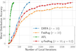
Figure 2: Comparing DRFA algorithm with AFL [35], q-FedAvg [25], and FedAvg on Fashion MNIST dataset with logistic regression. DRFA can achieve the same level of worst distribution accuracy, with fewer number of communication rounds, and hence, lower runtime. It also efficiently decreases the variance among the performance of different nodes with fewer communication rounds.

Comparison with baselines. From the algorithmic point of view, the AFL algorithm [35] is a special case of our DRFA algorithm, by setting the synchronization gap $\tau=1$. Hence, the first experiment suggests that we can increase the synchronization gap and achieve the same level of worst accuracy among distributions with fewer number of communications. In addition to AFL, q-FedAvg proposed by Li et al. [25] aims at balancing the performance among different clients, and hence, improving the worst distribution accuracy. In this part, we compare DRFA with AFL, q-FedAVG, and FedAvg.

To compare them, we run our algorithm, as well as AFL, q-FedAvg and FedAvg on Fashion MNIST dataset with logistic regression model on $10$ devices, each of which has access to one class of data. We set $\eta=0.1$ for all algorithms, $\gamma=8\times 10^{-3}$ for DRFA and AFL, and $q=0.2$ for q-FedAvg. The batch size is $50$ and synchronization gap is $\tau=10$. Figure 2 shows that AFL can reach to the $50\%$ worst distribution accuracy with fewer number of local iterations, because it updates the primal and dual variables at every iteration. However, Figure 2 shows that DRFA outperforms AFL, q-FedAvg and FedAvg in terms of number of communications, and subsequently, wall-clock time required to achieve the same level of worst distribution accuracy (due to much lower number of communication needed).

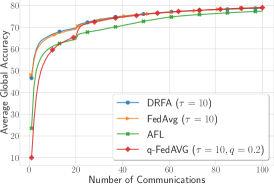
Figure 3: Averag global accuracy for each algorithm for $100$ rounds of communication. It shows that DRFA keeps the same level of global accuracy as FedAvg, while it boosts its worst performing distribution accuracy.

Note that, q-FedAvg has is very close to AFL in terms of communication rounds, but it is far behind it in terms of local computations. Also, note that FedAvg has the same computation complexity as DRFA and q-FedAvg at each round but cannot reach the $50\%$ accuracy even after $300$ rounds of communication. Similar to q-FedAvg, to show how different devices are performing, Figure 2 depicts the standard deviation among the accuracy of different clients, which shows the level of fairness of the learned model among different clients. It can be inferred that DRFA can achieve the same level as AFL and q-FedAvg with fewer number of communication rounds, making it more efficient. To compare the average performance of these algorithms, Figure 3 shows the global training accuracy of them over $100$ rounds of communication on Fashion MNIST with logistic regression, where DRFA performs as good as FedAvg in this regard. AFL needs more communication rounds to reach to the same level.

7 Conclusion

In this paper we propose a communication efficient scheme for distributionally robust federated model training. In addition, we give the first analysis of local SGD in distributed minimax optimization, under general smooth convex-linear, and nonconvex linear, strongly-convex-strongly-concave and nonconvex (PL-condition)-strongly concave settings. The experiments demonstrate the convergence of our method, and the distributional robustness of the learned model. The future work would be improving obtained convergence rates due to gap we observed compared to centralized case. Another interesting question worth exploring will be investigating variance reduction schemes to achieve faster rates, in particular for updating mixing parameter.

Broader Impact

This work advocates a distributionally robust algorithm for federated learning. The algorithmic solution is designed to preserve the privacy of users, while training a high quality model. The proposed algorithm tries to minimize the maximum loss among worst case distribution over clients’ data. Hence, we can ensure that even if the data distribution among users is highly heterogeneous, the trained model is reasonably good for everyone, and not benefiting only a group of clients. This will ensure the fairness in training a global model with respect to every user, and it is vitally important for critical decision making systems such as healthcare. In such a scenario, the model learned by simple algorithms such as FedAvg would have an inconsistent performance over different distributions, which is not acceptable. However, the resulting model from our algorithm will have robust performance over different distributions it has been trained on.

Appendix A Additional Experiments

In this section, we further investigate the effectiveness of the proposed DRFA algorithm. To do so, we use the Adult and Shakespeare datasets.

Experiments on Adult dataset. The Adult dataset contains census data, with the target of predicting whether the income is greater or less than $\$50K$. The data has $14$ features from age, race, gender, among others. It has $32561$ samples for training distributed across different groups of sensitive features. One of these sensitive features is gender, which has two groups of “male” and “female”. The other sensitive feature we will use is the race, where it has $5$ groups of “black”, “white”, “Asian-Pac-Islander”, “Amer-Indian-Eskimo”, and “other”. We can distribute data among nodes based on the value of these features, hence make it heterogeneously distributed.

For the first experiment, we distribute the training data across $10$ nodes, 5 of which contain only data from the female group and the other $5$ have the male group’s data. Since the size of different groups’ data is not equal, the data distribution is unbalanced among nodes. Figure 4 compares DRFA with AFL [35], q-FedAvg [25], and FedAvg [34] on the Adult dataset, where the data is distributed among the nodes based on the gender feature. We use logistic regression as the loss function, the learning rate is set to $0.1$ and batch size is $50$ for all algorithms, $\gamma$ is set to $0.2$ for both DRFA and AFL, and $q=0.5$ is tuned for the best results for q-FedAvg. The worst distribution or node accuracy during the communication rounds shows that DRFA can achieve the same level of worst accuracy with a far fewer number of communication rounds, and hence, less overall wall-clock time. However, AFL computational cost is less than that of DRFA. Between each communication rounds DRFA, q-FedAvg and FedAvg have $10$ update steps. FedAvg after the same number of communications as AFL still cannot reach the same level of worst accuracy. Figure 4 shows the standard deviation of accuracy among different nodes as a measure for the fairness of algorithms. It can be inferred that DRFA efficiently decreases the variance with a much fewer number of communication rounds with respect to other algorithms.

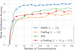
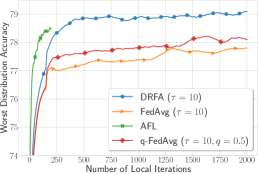
Figure 4: Comparing the worst distribution accuracy on DRFA, AFL, q-FedAvg, and FedAVG on the Adult dataset. We have $10$ nodes, and data is distributed among them based on the gender feature. The loss function is logistic regression. DRFA needs a fewer number of communications to reach the same worst distribution accuracy than the AFL and q-FedAvg algorithms. Also, DRFA efficiently decreases the variance of the performance of different clients.

Next, we distribute the Adult data among clients based on the “race” feature, which has $5$ different groups. Again the size of data among these groups is not equal and makes the distribution unbalanced. We distribute the data among $10$ nodes, where every node has only data from one group of the race feature. For this experiment, we use a nonconvex loss function, where the model is a multilayer perceptron (MLP) with $2$ hidden layers, each with $50$ neurons. The first layer has $14$ and the last layer has $2$ neurons. The learning rate is set to $0.1$ and batch size is $50$ for all algorithms, the $\gamma$ is set to $0.2$ for DRFA and AFL, and the $q$ parameter in q-FedAvg is tuned for $0.5$. Figure 5 shows the results of this experiment, where again, DRFA can achieve the same worst-case accuracy with a much fewer number of communications than AFL and q-FedAvg. In this experiment, with the same number of local iterations, AFL still cannot reach to the DRFA performance. In addition, the variance on the performance of different clients in Figure 5 suggests that DRFA is more successful than q-FedAvg to balance the performance of clients.

Figure 5: Comparing the worst distribution accuracy on DRFA, AFL, q-FedAvg, and FedAvg with the Adult dataset. We have $10$ nodes, and data is distributed among them based on the race feature. The model is an MLP with $2$ hidden layers, each with $50$ neurons and a cross-entropy loss function. DRFA needs a fewer number of communications to reach the same worst distribution accuracy than the AFL and q-FedAvg algorithms. Moreover, DRFA is more efficient in reducing the performance variance among different clients than q-FedAvg.

Experiments on Shakespeare dataset. Now, we run the same experiments on the Shakespeare dataset. This dataset contains the scripts from different Shakespeare’s plays divided based on the character in each play. The task is to predict the next character in the text, providing the preceding characters. For this experiment, we use $100$ clients’ data to train our RNN model. The RNN model comprises an embedding layer from $86$ characters to $50$, followed by a layer of GRU [5] with $50$ units. The output is going through a fully connected layer with an output size of $86$ and a cross-entropy loss function. We use the batch size of $2$ with $50$ characters in each batch. The learning rate is optimized to $0.8$ for the FedAvg and used for all algorithms. The $\gamma$ is tuned to the $0.01$ for AFL and DRFA, and $q=0.1$ is the best for the q-FedAvg. Figure 6 shows the results of this experiment on the Shakespeare dataset. It can be seen that DRFA and FedAvg can reach to the same worst distribution accuracy compared to AFL and q-FedAvg. The reason that FedAvg is working very well in this particular dataset is that the distribution of data based on the characters in the plays does not make it heterogeneous. In settings close to homogeneous distribution, FedAvg can achieve the best results, with DRFA having a slight advantage over that.

Figure 6: Comparing different algorithms on training an RNN on Shakespeare dataset using $100$ clients. DRFA and FedAvg outperform the other two algorithms in terms of communication efficiency, however, AFL can achieve the same level with lower computation cost. In the average performance, AFL requires much more communication to reach to the same level as FedAvg and DRFA.

Appendix B Formal Convergence Theory for Alternative Algorithm in Regularized Case

Here, we will present the formal convergence theory of the algorithm we described in Section 5.2, where we use full batch gradient ascent to update $\boldsymbol{\lambda}^{(s)}$. To do so, the server sends the current global model $\bar{\boldsymbol{w}}^{(s)}$ to all clients and each client evaluates the global model on its local data shards and send $f_{i}(\bar{\boldsymbol{w}}^{(s)})$ back to the server. Then the server can compute the full gradient over dual parameter $\boldsymbol{\lambda}$ and take a gradient ascent (GA) step to update it. The algorithm is named DRFA-GA and described in Algorithm 3. We note that DRFA-GA can be considered as communication-efficient variant of AFL, but without sampling clients to evaluate the gradient at dual parameter. We conduct the convergence analysis on the setting where the regularized term is strongly-concave in $\boldsymbol{\lambda}$, and loss function is strongly-convex and nonconvex but satisfying Polyak-Łojasiewicz (PL) condition in $\boldsymbol{w}$. So, our theory includes strongly-convex-strongly-concave and nonconvex (PL condition)-strongly-concave cases.

Strongly-Convex-Strongly-Concave case.  We start by stating the convergence rate when the individual local objectives are strongly convex and the regularizer $g(\boldsymbol{\lambda})$ is strongly concave in $\boldsymbol{\lambda}$, making the global objective $F(\boldsymbol{w},\boldsymbol{\lambda}):=\sum_{i=1}^{N}\lambda_{i}f_{i}(\boldsymbol{w})+g(\boldsymbol{\lambda})$ also strongly concave in $\boldsymbol{\lambda}$.

Theorem 5.

Let each local function $f_{i}$ be $\mu$-strongly convex, and global function $F$ is $\mu$-strongly concave in $\boldsymbol{\lambda}$. Under Assumptions 1, 2,3,4, if we optimize (5) using the DRFA-GA (Algorithm 3) with synchronization gap $\tau$, choosing learning rates as $\eta=\frac{4\log T}{\mu T}$ and $\gamma=\frac{1}{L}$ and $T\geq\frac{16\alpha\log T}{\mu}$, where $\alpha=\kappa L+L$, using the averaging scheme $\hat{\boldsymbol{w}}=\frac{2}{mT}\sum_{t=T/2}^{T}\sum_{i\in{\mathcal{D}^{(\left\lfloor\frac{t}{\tau}\right\rfloor)}}}\boldsymbol{w}^{(t)}_{i}$ we have:

$$\mathbb{E}[\Phi(\hat{\boldsymbol{w}})-\Phi(\boldsymbol{w}^{*})]=\tilde{O}\left(\frac{\mu D_{\mathcal{W}}^{2}}{T}+\frac{\kappa^{2}L\tau D_{\Lambda}^{2}}{T}+\frac{\sigma_{w}^{2}+G_{w}^{2}}{\mu mT}+\frac{\kappa^{2}\tau^{2}(\sigma_{w}^{2}+\Gamma)}{\mu T^{2}}+\frac{\kappa^{6}\tau^{2}G_{w}^{2}}{\mu T^{2}}\right),$$

where $\kappa=L/\mu$, and $\boldsymbol{w}^{*}$ is the minimizer of $\Phi$.

Proof.

The proof is given in Section F. ∎

Corollary 1.

Continuing with Theorem 5, if we choose $\tau=\sqrt{T/m}$, we recover the rate:

$$\mathbb{E}[\Phi(\hat{\boldsymbol{w}})-\Phi(\boldsymbol{w}^{*})]=\tilde{O}\left(\frac{\kappa^{2}LD_{\Lambda}^{2}}{\sqrt{mT}}+\frac{\mu D_{\mathcal{W}}^{2}}{T}+\frac{\kappa^{2}(\sigma_{w}^{2}+\Gamma)+\kappa^{6}G_{w}^{2}}{\mu mT}\right).$$

Here we obtain $\tilde{O}\left(\frac{\tau}{T}\right)$ rate in Theorem 5. If we choose $\tau=1$, which is fully synchronized SGD, then we recover the same rate $\tilde{O}\left(\frac{1}{T}\right)$ as in vanilla agnostic federated learning [35]. If we choose $\tau$ to be $O(\sqrt{T/m})$, we recover the rate $\tilde{O}\left(\frac{1}{\sqrt{mT}}+\frac{1}{mT}\right)$, which can achieve linear speedup with respect to number of sampled workers. The dependency on gradient dissimilarity $\Gamma$ shows that the data heterogeneity will slow down the rate, but will not impact the dominating term.

0:  $N$ clients , synchronization gap $\tau$, total number of iterations $T$, $S=T/\tau$, learning rates $\eta$, $\gamma$, sampling size $m$, initial model $\bar{\boldsymbol{w}}^{(0)}$ and initial $\boldsymbol{\lambda}^{(0)}$.

0:  Final solutions $\hat{\boldsymbol{w}}=\frac{2}{mT}\sum_{t=T/2}^{T}\sum_{i\in{\mathcal{D}^{(\lfloor\frac{t}{\tau}\rfloor)}}}\boldsymbol{w}^{(t)}_{i}$, $\hat{\boldsymbol{\lambda}}=\frac{1}{S}\sum_{s=0}^{S-1}\boldsymbol{\lambda}^{(s)}$, or (2) $\boldsymbol{w}^{T}$, $\boldsymbol{\lambda}^{S}$.

1:  for  $s=0$ to $S-1$  do

2:     Server samples $\mathcal{D}^{(s)}\subset[N]$ according to $\boldsymbol{\lambda}^{(s)}$ with size of $m$

3:     Server broadcasts $\bar{\boldsymbol{w}}^{(s)}$ to all clients $i\in\mathcal{D}^{(s)}$

4:     for clients $i\in\mathcal{D}^{(s)}$ parallel do 5:        Client sets $\boldsymbol{w}_{i}^{(s\tau)}=\bar{\boldsymbol{w}}^{(s)}$ 6:        for $t=s\tau,\ldots,(s+1)\tau-1$ do 7:           $\boldsymbol{w}^{(t+1)}_{i}=\prod_{\mathcal{W}}\left(\boldsymbol{w}^{(t)}_{i}-\eta\nabla f_{i}(\boldsymbol{w}^{(t)}_{i};\xi^{(t)}_{i})\right)$ 8:        end for 9:     end for 10:     Client $i\in\mathcal{D}^{(s)}$ sends $\boldsymbol{w}^{((s+1)\tau)}_{i}$ back to the server 11:     Server sends $\bar{\boldsymbol{w}}^{(s)}$ to all clients // Update $\boldsymbol{\lambda}$ 12:     Each client $i\in[N]$ evaluates $\bar{\boldsymbol{w}}^{(s)}$ on its local data and sends $f_{i}(\bar{\boldsymbol{w}}^{(s)})$ back to server 13:     Server updates $\boldsymbol{\lambda}^{(s+1)}=\prod_{\Lambda}\left(\boldsymbol{\lambda}^{(s)}+\gamma\nabla_{\boldsymbol{\lambda}}F\left(\bar{\boldsymbol{w}}^{(s)},\boldsymbol{\lambda}^{(s)}\right)\right)$

14:     Server computes $\bar{\boldsymbol{w}}^{(s+1)}=\frac{1}{m}\sum_{i\in\mathcal{D}^{(s)}}\boldsymbol{w}^{((s+1)\tau)}_{i}$

15:  end for

Algorithm 3 Distributionally Robust Federated Averaging: Gradient Ascent (DRFA-GA)

Nonconvex (PL condition)-Strongly-Concave Setting. We provide the convergence analysis under the condition where $F$ is nonconvex but satisfies PL condition in $\boldsymbol{w}$, and strongly concave in $\boldsymbol{\lambda}$. In the constraint problem, to prove the convergence, we have to consider a generalization of PL condition [17] as formally stated below.

Definition 4 (($\mu$,$\eta$)-generalized Polyak-Łojasiewicz (PL)).

The global objective function $F(\cdot,\boldsymbol{\lambda})$ is differentiable and satisfies the ($\mu$,$\eta$)-generalized Polyak-Łojasiewicz condition with constant $\mu$ if the following holds:

$$\frac{1}{2\eta^{2}}\left\|\boldsymbol{w}-\prod_{\mathcal{W}}\left(\boldsymbol{w}-\eta\nabla_{\boldsymbol{w}}F(\boldsymbol{w},\boldsymbol{\lambda})\right)\right\|_{2}^{2}\geq\mu(F(\boldsymbol{w},\boldsymbol{\lambda})-\min_{\boldsymbol{w}^{\prime}\in\mathcal{W}}F(\boldsymbol{w}^{\prime},\boldsymbol{\lambda})),\forall\boldsymbol{\lambda}\in\Lambda$$

.

Remark 1.

When the constraint is absent, it reduces to vanilla PL condition [17]. The similar generalization of PL condition is also mentioned in [17], where they introduce a variant of PL condition to prove the convergence of proximal gradient method. Also we will show that, if $F$ satisfies $\mu$-PL condition in $\boldsymbol{w}$, $\Phi(\boldsymbol{w})$ also satisfies $\mu$-PL condition.

We now proceed to provide the global convergence of $\Phi$ in this setting.

Theorem 6.

Let global function $F$ satisfy ($\mu$,$\eta$)-generalized PL condition in $\boldsymbol{w}$ and $\mu$-strongly-concave in $\boldsymbol{\lambda}$. Under Assumptions 1,2,3,4, if we optimize (5) using the DRFA-GA (Algorithm 3) with synchronization gap $\tau$, choosing learning rates $\eta=\frac{4\log T}{\mu T}$, $\gamma=\frac{1}{L}$ and $m\geq T$, with the total iterations satisfying $T\geq\frac{8\alpha\log T}{\mu}$ where $\alpha=L+\kappa L$, $\kappa=\frac{L}{\mu}$, we have:

$$\mathbb{E}\left[\Phi(\boldsymbol{w}^{(T)})-\Phi(\boldsymbol{w}^{*})\right] \leq O\left(\frac{\Phi(\boldsymbol{w}^{(0)})-\Phi(\boldsymbol{w}^{*})}{T}\right)+\tilde{O}\left(\frac{\sigma_{w}^{2}+G_{w}^{2}}{\mu T}\right)+\tilde{O}\left(\frac{\kappa^{2}L\tau D_{\Lambda}^{2}}{T}\right)$$

$$\quad+\tilde{O}\left(\frac{\kappa^{6}\tau^{2}G_{w}^{2}}{\mu T^{2}}\right)+\tilde{O}\left(\frac{\kappa^{2}\tau^{2}(\sigma_{w}^{2}+\Gamma)}{\mu T^{2}}\right).$$

where $\boldsymbol{w}^{*}\in\arg\min_{\boldsymbol{w}\in\mathcal{W}}\Phi(\boldsymbol{w})$.

Proof.

The proof is given in Section G. ∎

Corollary 2.

Continuing with Theorem 6, if we choose $\tau=\sqrt{T/m}$, we recover the rate:

$$\mathbb{E}[\Phi(\hat{\boldsymbol{w}})-\Phi(\boldsymbol{w}^{*})]=\tilde{O}\left(\frac{\kappa^{2}LD_{\Lambda}^{2}}{\sqrt{T}}+\frac{\Phi(\boldsymbol{w}^{(0)})-\Phi(\boldsymbol{w}^{*})}{T}+\frac{\kappa^{2}(\sigma_{w}^{2}+\Gamma)+\kappa^{6}G_{w}^{2}}{\mu T}\right).$$

We obtain $\tilde{O}\left(\frac{\tau}{T}\right)$ convergence rate here, slightly worse than that of strongly-convex-strongly-concave case. We also get linear speedup in the number of sampled workers if properly choose $\tau$. The best known result of non-distributionally robust version of FedAvg on PL condition is $O(\frac{1}{T})$ [12], with $O(T^{1/3})$ communication rounds. It turns out that we trade some convergence rate to guarantee a worst case performance. We would like to mention that, here we require $m$, the number of sampled clients to be a large number, which is the imperfection of our analysis. However, we would note that, this is similar to the analysis in [10] for projected SGD on constrained nonconvex minimization problems, where it is required to employ growing mini-batch sizes with iterations to guarantee convergence to a first-order stationary point (i.e., imposing a constraint on minibatch size based on target accuracy $\epsilon$ which plays a similar rule to $m$ in our case).

Appendix C Proof of Convergence of DRFA for Convex Losses (Theorem 1)

In this section we will present the proof of Theorem 1, which states the convergence of DRFA in convex-linear setting.

C.1 Preliminary

Before delving into the proof, let us introduce some useful variables and lemmas for ease of analysis. We define a virtual sequence $\{\boldsymbol{w}^{(t)}\}_{t=1}^{T}$ that will be used in our proof, and we also define some intermediate variables:

$$\boldsymbol{w}^{(t)} =\frac{1}{m}\sum_{i\in{\mathcal{D}^{(\lfloor\frac{t}{\tau}\rfloor)}}}\boldsymbol{w}^{(t)}_{i},$$ (average model of selected devices)

$$\bar{\boldsymbol{u}}^{(t)} =\frac{1}{m}\sum_{i\in\mathcal{D}^{(\lfloor\frac{t}{\tau}\rfloor)}}\nabla f_{i}(\boldsymbol{w}^{(t)}_{i}),$$ (average full gradient of selected devices)

$$\boldsymbol{u}^{(t)} =\frac{1}{m}\sum_{i\in{\mathcal{D}^{(\lfloor\frac{t}{\tau}\rfloor)}}}\nabla f_{i}(\boldsymbol{w}^{(t)}_{i};\xi^{(t)}_{i})$$ (average stochastic gradient of selected devices)

$$\bar{\boldsymbol{v}}^{(t)} =\nabla_{\boldsymbol{\lambda}}F(\boldsymbol{w}^{(t)},\boldsymbol{\lambda})=\left[f_{1}(\boldsymbol{w}^{(t)}),\ldots,f_{N}(\boldsymbol{w}^{(t)})\right]$$ (full gradient w.r.t. dual)

$$\bar{\Delta}_{s} =\sum_{t=s\tau+1}^{(s+1)\tau}\gamma\bar{\boldsymbol{v}}^{(t)},$$

$$\Delta_{s} =\tau\gamma\boldsymbol{v},$$ (see below)

$$\delta^{(t)} =\frac{1}{m}\sum_{i\in\mathcal{D}^{(\lfloor\frac{t}{\tau}\rfloor)}}\left\|\boldsymbol{w}^{(t)}_{i}-\boldsymbol{w}^{(t)}\right\|^{2},$$

where $\boldsymbol{v}\in\mathbb{R}^{N}$ is the stochastic gradient for dual variable generated by Algorithm 1 for updating $\boldsymbol{\lambda}$, such that ${v}_{i}=f_{i}(\boldsymbol{w}^{(t^{\prime})};\xi_{i})$ for $i\in\mathcal{U}\subset[N]$ where $\xi_{i}$ is stochastic minibatch sampled from $i$th local data shard, and $t^{\prime}$ is the snapshot index sampled from $s\tau+1$ to $(s+1)\tau$.

C.2 Overview of the Proof

The proof techniques consist of analyzing the one-step progress for the virtual iterates $\boldsymbol{w}^{(t+1)}$ and $\boldsymbol{\lambda}^{(s+1)}$, however periodic decoupled updating along with sampling makes the analysis more involved compared to fully synchronous primal-dual schemes for minimax optimization. Let us start from analyzing one iteration on $\boldsymbol{w}$. From the updating rule we can show that

$$\mathbb{E}\|\boldsymbol{w}^{(t+1)}-\boldsymbol{w}\|^{2} \leq\mathbb{E}\|\boldsymbol{w}^{(t)}-\boldsymbol{w}\|^{2}-2\eta\mathbb{E}\left[F(\boldsymbol{w}^{(t)},\boldsymbol{\lambda}^{(\lfloor\frac{t}{\tau}\rfloor)})-F(\boldsymbol{w},\boldsymbol{\lambda}^{(\lfloor\frac{t}{\tau}\rfloor)})\right]$$

$$\quad+L\eta\mathbb{E}\left[\delta^{(t)}\right]+\eta^{2}\mathbb{E}\|\bar{\boldsymbol{u}}^{(t)}-\boldsymbol{u}^{(t)}\|^{2}+\eta^{2}G_{w}^{2}.$$

Note that, similar to analysis of local SGD, e.g.,  [44], the key question is how to bound the deviation $\delta^{(t)}$ between local and (virtual) averaged model. By the definition of gradient dissimilarity, we establish that:

$$\frac{1}{T}\sum_{t=0}^{T}\mathbb{E}\left[\delta^{(t)}\right]=10\eta^{2}\tau^{2}\left(\sigma_{w}^{2}+\frac{\sigma_{w}^{2}}{m}+\Gamma\right).$$

It turns out the deviation can be upper bounded by variance of stochastic graident, and the gradient dissimilarity. The latter term controls how heterogenous the local component functions are, and it becomes zero when all local functions are identical, which means we are doing minibatch SGD on the same objective function in parallel.

Now we switch to the one iteration analysis on $\boldsymbol{\lambda}$:

$$\mathbb{E}\|\boldsymbol{\lambda}^{(s+1)}-\boldsymbol{\lambda}\|^{2} \leq\mathbb{E}\|\boldsymbol{\lambda}^{(s)}-\boldsymbol{\lambda}\|^{2}$$

$$\quad-\sum_{t=s\tau+1}^{(s+1)\tau}\mathbb{E}[2\gamma(F(\boldsymbol{w}^{(t)},\boldsymbol{\lambda}^{(s)})-F(\boldsymbol{w}^{(t)},\boldsymbol{\lambda}))]+\mathbb{E}\|\bar{\Delta}_{s}\|^{2}+\mathbb{E}\|\Delta_{s}-\bar{\Delta}_{s}\|^{2}.$$

It suffices to bound the variance of $\Delta_{s}$. Using the identity of independent variables we can prove:

$$\mathbb{E}[\|\Delta_{s}-\bar{\Delta}_{s}\|^{2}]\leq\gamma^{2}\tau^{2}\frac{\sigma_{\lambda}^{2}}{m}.$$

It shows that the variance depends quadratically on $\tau$, and can achieve linear speed up with respect to the number of sampled workers. Putting all pieces together, and doing the telescoping sum will yield the result in Theorem 1.

C.3 Proof of Technical Lemmas

In this section we are going to present some technical lemmas that will be used in the proof of Theorem 1.

Lemma 1.

The stochastic gradient $\boldsymbol{u}^{(t)}$ is unbiased, and its variance is bounded, which implies:

$$\mathbb{E}_{\xi_{i}^{(t)},\mathcal{D}^{(\lfloor\frac{t}{\tau}\rfloor)}}\left[\boldsymbol{u}^{(t)}\right] =\mathbb{E}_{\mathcal{D}^{(\lfloor\frac{t}{\tau}\rfloor)}}\left[\bar{\boldsymbol{u}}^{(t)}\right]=\mathbb{E}\left[\sum_{i=1}^{N}\lambda^{(\lfloor\frac{t}{\tau}\rfloor)}_{i}\nabla f_{i}(\boldsymbol{w}^{(t)}_{i})\right],$$

$$\mathbb{E}\left[\|\boldsymbol{u}^{(t)}-\bar{\boldsymbol{u}}^{(t)}\|^{2}\right] =\frac{\sigma^{2}_{w}}{m}.$$

Proof.

The unbiasedness is due to the fact that we sample the clients according to $\boldsymbol{\lambda}^{(\lfloor\frac{t}{\tau}\rfloor)}$. The variance term is due to the identity $\mathrm{Var}(\sum_{i=1}^{m}\boldsymbol{X}_{i})=\sum_{i=1}^{m}\mathrm{Var}(\boldsymbol{X}_{i})$. ∎

Lemma 2.

The stochastic gradient at $\boldsymbol{\lambda}$ generated by Algorithm 1 is unbiased, and its variance is bounded, which implies:

$$\mathbb{E}[\Delta_{s}]=\bar{\Delta}_{s},\quad\quad\mathbb{E}[\|\Delta_{s}-\bar{\Delta}_{s}\|^{2}]\leq\gamma^{2}\tau^{2}\frac{\sigma_{\lambda}^{2}}{m}.$$ (6)

Proof.

The unbiasedness is due to we sample the workers uniformly. The variance term is due to the identity $\mathrm{Var}(\sum_{i=1}^{m}\boldsymbol{X}_{i})=\sum_{i=1}^{m}\mathrm{Var}(\boldsymbol{X}_{i})$. ∎

Lemma 3 (One Iteration Primal Analysis).

For DRFA, under the same conditions as in Theorem 1, for all $\boldsymbol{w}\in\mathcal{W}$, the following holds:

$$\mathbb{E}\|\boldsymbol{w}^{(t+1)}-\boldsymbol{w}\|^{2} \leq\mathbb{E}\|\boldsymbol{w}^{(t)}-\boldsymbol{w}\|^{2}-2\eta\mathbb{E}\left[F(\boldsymbol{w}^{(t)},\boldsymbol{\lambda}^{(\lfloor\frac{t}{\tau}\rfloor)})-F(\boldsymbol{w},\boldsymbol{\lambda}^{(\lfloor\frac{t}{\tau}\rfloor)})\right]$$

$$\quad+L\eta\mathbb{E}\left[\delta^{(t)}\right]+\eta^{2}\mathbb{E}\|\bar{\boldsymbol{u}}^{(t)}-\boldsymbol{u}^{(t)}\|^{2}+\eta^{2}G_{w}^{2}.$$

Proof.

From the updating rule we have:

$$\mathbb{E}\|\boldsymbol{w}^{(t+1)}-\boldsymbol{w}\|^{2} =\mathbb{E}\left\|\prod_{\mathcal{W}}(\boldsymbol{w}^{(t)}-\eta\boldsymbol{u}^{(t)})-\boldsymbol{w}\right\|^{2}\leq\mathbb{E}\|\boldsymbol{w}^{(t)}-\eta\bar{\boldsymbol{u}}^{(t)}-\boldsymbol{w}\|^{2}+\eta^{2}\mathbb{E}\|\bar{\boldsymbol{u}}^{(t)}-\boldsymbol{u}^{(t)}\|^{2}$$

$$\leq\mathbb{E}\|\boldsymbol{w}^{(t)}-\boldsymbol{w}^{*}\|^{2}+\underbrace{\mathbb{E}[-2\eta\langle\bar{\boldsymbol{u}}^{(t)},\boldsymbol{w}^{(t)}-\boldsymbol{w}^{*}\rangle]}_{T_{1}}+\underbrace{\eta^{2}\mathbb{E}\|\bar{\boldsymbol{u}}^{(t)}\|^{2}}_{T_{2}}+\mathbb{E}\|\bar{\boldsymbol{u}}^{(t)}-\boldsymbol{u}^{(t)}\|^{2}$$ (7)

We are going to bound $T_{1}$ first:

$$T_{1} =\mathbb{E}_{\mathcal{D}^{(\lfloor\frac{t}{\tau}\rfloor)}}\left[\frac{1}{m}\sum_{i\in\mathcal{D}^{(\lfloor\frac{t}{\tau}\rfloor)}}\left[-2\eta\left\langle\nabla f_{i}(\boldsymbol{w}^{(t)}_{i}),\boldsymbol{w}^{(t)}-\boldsymbol{w}^{(t)}_{i}\right\rangle-2\eta\left\langle\nabla f_{i}(\boldsymbol{w}^{(t)}_{i}),\boldsymbol{w}^{(t)}_{i}-\boldsymbol{w}^{*}\right\rangle\right]\right]$$ (8)

$$\leq\mathbb{E}_{\mathcal{D}^{(\lfloor\frac{t}{\tau}\rfloor)}}\left[2\eta\frac{1}{m}\sum_{i\in\mathcal{D}^{(\lfloor\frac{t}{\tau}\rfloor)}}\left[f_{i}(\boldsymbol{w}^{(t)}_{i})-f_{i}(\boldsymbol{w}^{(t)})+\frac{L}{2}\|\boldsymbol{w}^{(t)}-\boldsymbol{w}^{(t)}_{i}\|^{2}+f_{i}(\boldsymbol{w})-f_{i}(\boldsymbol{w}^{(t)}_{i})\right]\right]$$ (9)

$$=-2\eta\mathbb{E}\left[\sum_{i=1}^{N}\lambda^{(\lfloor\frac{t}{\tau}\rfloor)}_{i}f_{i}(\boldsymbol{w}^{(t)})-\lambda^{(\lfloor\frac{t}{\tau}\rfloor)}_{i}f_{i}(\boldsymbol{w})\right]+L\eta\mathbb{E}\left[\delta^{(t)}\right]$$

$$=-2\eta\mathbb{E}\left[F(\boldsymbol{w}^{(t)},\boldsymbol{\lambda}^{(\lfloor\frac{t}{\tau}\rfloor)})-F(\boldsymbol{w},\boldsymbol{\lambda}^{(\lfloor\frac{t}{\tau}\rfloor)})\right]+L\eta\mathbb{E}\left[\delta^{(t)}\right],$$

where from (8) to (9) we use the smoothness and convexity properties.

We then turn to bounding $T_{2}$ as follows:

$$T_{2}=\eta^{2}\mathbb{E}\left\|\frac{1}{m}\sum_{i\in\mathcal{D}^{(\lfloor\frac{t}{\tau}\rfloor)}}\nabla f_{i}(\boldsymbol{w}^{(t)}_{i})\right\|^{2}\leq\eta^{2}\frac{1}{m}\sum_{i\in\mathcal{D}^{(\lfloor\frac{t}{\tau}\rfloor)}}\mathbb{E}\left\|\nabla f_{i}(\boldsymbol{w}^{(t)}_{i})\right\|^{2}\leq\eta^{2}G_{w}^{2}.$$

Plugging $T_{1}$ and $T_{2}$ back to (7) gives:

$$\mathbb{E}\|\boldsymbol{w}^{(t+1)}-\boldsymbol{w}\|^{2} \leq\mathbb{E}\|\boldsymbol{w}^{(t)}-\boldsymbol{w}\|^{2}-2\eta\mathbb{E}\left[F(\boldsymbol{w}^{(t)},\boldsymbol{\lambda}^{(\lfloor\frac{t}{\tau}\rfloor)})-F(\boldsymbol{w},\boldsymbol{\lambda}^{(\lfloor\frac{t}{\tau}\rfloor)})\right]$$

$$\quad+L\eta\mathbb{E}\left[\delta^{(t)}\right]+\eta^{2}\mathbb{E}\|\bar{\boldsymbol{u}}^{(t)}-\boldsymbol{u}^{(t)}\|^{2}+\eta^{2}G_{w}^{2},$$

thus concluding the proof. ∎

The following lemma bounds the deviation between local models and (virtual) global average model over sampled devices over $T$ iterations. We note that the following result is general and will be used in all variants.

Lemma 4 (Bounded Squared Deviation).

For DRFA, DRFA-Prox and DRFA-GA algorithms, the expected average squared norm distance of local models $\boldsymbol{w}^{(t)}_{i},i\in\mathcal{D}^{(\lfloor\frac{t}{\tau}\rfloor)}$ and $\boldsymbol{w}^{(t)}$ is bounded as follows:

$$\frac{1}{T}\sum_{t=0}^{T}\mathbb{E}\left[\delta^{(t)}\right]\leq 10\eta^{2}\tau^{2}\left(\sigma_{w}^{2}+\frac{\sigma_{w}^{2}}{m}+\Gamma\right).$$

where expectation is taken over sampling of devices at each iteration.

Proof.

Consider $s\tau\leq t\leq(s+1)\tau$. Recall that, we only perform the averaging based on a uniformly sampled subset of workers $\mathcal{D}^{(\lfloor\frac{t}{\tau}\rfloor)}$ of $[N]$. Following the updating rule we have:

$$\mathbb{E}[\delta^{(t)}] =\mathbb{E}\left[\frac{1}{m}\sum_{i\in\mathcal{D}^{(\lfloor\frac{t}{\tau}\rfloor)}}\|\boldsymbol{w}^{(t)}_{i}-\boldsymbol{w}^{(t)}\|^{2}\right]$$

$$\leq\mathbb{E}\left[\frac{1}{m}\sum_{i\in\mathcal{D}^{(\lfloor\frac{t}{\tau}\rfloor)}}\mathbb{E}\left\|\boldsymbol{w}^{(s\tau)}-\sum_{r=s\tau}^{t-1}\eta\nabla f_{i}(\boldsymbol{w}^{(r)}_{i};\xi_{i}^{(r)})-\left(\boldsymbol{w}^{(s\tau)}-\frac{1}{m}\sum_{i^{\prime}\in\mathcal{D}}\sum_{r=s\tau}^{t-1}\eta\nabla f_{i^{\prime}}(\boldsymbol{w}^{(r)}_{i^{\prime}};\xi_{i^{\prime}}^{(r)})\right)\right\|^{2}\right]$$

$$=\mathbb{E}\left[\frac{1}{m}\sum_{i\in\mathcal{D}^{(\lfloor\frac{t}{\tau}\rfloor)}}\left\|\sum_{r=s\tau}^{t-1}\eta\nabla f_{i}(\boldsymbol{w}^{(r)}_{i};\xi_{i}^{(r)})-\frac{1}{m}\sum_{i^{\prime}\in\mathcal{D}^{(\lfloor\frac{t}{\tau}\rfloor)}}\sum_{r=s\tau}^{t-1}\eta\nabla f_{i^{\prime}}(\boldsymbol{w}^{(r)}_{i^{\prime}};\xi_{i^{\prime}}^{(r)})\right\|^{2}\right]$$

$$\leq\mathbb{E}\left[\frac{1}{m}\sum_{i\in\mathcal{D}^{(\lfloor\frac{t}{\tau}\rfloor)}}\eta^{2}\tau\sum_{r=s\tau}^{(s+1)\tau}\left\|\nabla f_{i}(\boldsymbol{w}^{(r)}_{i};\xi_{i}^{(r)})-\frac{1}{m}\sum_{i^{\prime}\in\mathcal{D}^{(\lfloor\frac{t}{\tau}\rfloor)}}\nabla f_{i^{\prime}}(\boldsymbol{w}^{(r)}_{i^{\prime}};\xi_{i^{\prime}}^{(r)})\right\|^{2}\right]$$

$$=\eta^{2}\tau\mathbb{E}\left[\frac{1}{m}\sum_{i\in\mathcal{D}^{(\lfloor\frac{t}{\tau}\rfloor)}}\sum_{r=s\tau}^{(s+1)\tau}\left\|\nabla f_{i}(\boldsymbol{w}^{(r)}_{i};\xi_{i}^{(r)})-\nabla f_{i}(\boldsymbol{w}^{(r)}_{i})+\nabla f_{i}(\boldsymbol{w}^{(r)}_{i})-\nabla f_{i}(\boldsymbol{w}^{(r)})\vphantom{-\frac{1}{m}\sum_{i^{\prime}\in\mathcal{D}^{(\lfloor\frac{t}{\tau}\rfloor)}}\nabla f_{i^{\prime}}(\boldsymbol{w}^{(r)}_{i^{\prime}})}\right.\right.$$

$$\qquad\qquad\left.\left.+\nabla f_{i}(\boldsymbol{w}^{(r)})-\frac{1}{m}\sum_{i^{\prime}\in\mathcal{D}^{(\lfloor\frac{t}{\tau}\rfloor)}}\nabla f_{i^{\prime}}(\boldsymbol{w}^{(r)})+\frac{1}{m}\sum_{i^{\prime}\in\mathcal{D}^{(\lfloor\frac{t}{\tau}\rfloor)}}\nabla f_{i^{\prime}}(\boldsymbol{w}^{(r)})\right.\right.$$

$$\qquad\qquad\left.\left.-\frac{1}{m}\sum_{i^{\prime}\in\mathcal{D}^{(\lfloor\frac{t}{\tau}\rfloor)}}\nabla f_{i^{\prime}}(\boldsymbol{w}^{(r)}_{i^{\prime}})+\frac{1}{m}\sum_{i^{\prime}\in\mathcal{D}^{(\lfloor\frac{t}{\tau}\rfloor)}}\nabla f_{i^{\prime}}(\boldsymbol{w}^{(r)}_{i^{\prime}})-\frac{1}{m}\sum_{i^{\prime}\in\mathcal{D}^{(\lfloor\frac{t}{\tau}\rfloor)}}\nabla f_{i^{\prime}}(\boldsymbol{w}^{(r)}_{i^{\prime}};\xi_{i^{\prime}}^{(r)})\right\|^{2}\right]$$ (10)

Applying Jensen’s inequality to split the norm yields:

$$\mathbb{E}[\delta^{(t)}] \leq 5\eta^{2}\tau\sum_{r=s\tau}^{(s+1)\tau}\left(\sigma_{w}^{2}+L^{2}\mathbb{E}\left[\frac{1}{m}\sum_{i\in\mathcal{D}^{(\lfloor\frac{t}{\tau}\rfloor)}}\left\|\boldsymbol{w}^{(r)}_{i}-\boldsymbol{w}^{(r)}\right\|^{2}\right]+L^{2}\mathbb{E}\left[\frac{1}{m}\sum_{i^{\prime}\in\mathcal{D}^{(\lfloor\frac{t}{\tau}\rfloor)}}\left\|\boldsymbol{w}^{(r)}_{i^{\prime}}-\boldsymbol{w}^{(r)}\right\|^{2}\right]\right.$$

$$\qquad\qquad\left.+\mathbb{E}\left[\frac{1}{m}\sum_{i^{\prime}\in\mathcal{D}^{(\lfloor\frac{t}{\tau}\rfloor)}}\left\|\nabla f_{i}(\boldsymbol{w}^{(r)})-\nabla f_{i^{\prime}}(\boldsymbol{w}^{(r)})\right\|^{2}\right]+\frac{\sigma_{w}^{2}}{m}\right)$$ (11)

$$\leq 5\eta^{2}\tau\sum_{r=s\tau}^{(s+1)\tau}\left(\sigma^{2}_{w}+2L^{2}\mathbb{E}[\delta^{(r)}]+\Gamma+\frac{\sigma^{2}_{w}}{m}\right),$$ (12)

where from (10) to (11) we use the Jensen’s inequality.

Now we sum (12) over $t=s\tau$ to $(s+1)\tau$ to get:

$$\sum_{t=s\tau}^{(s+1)\tau}\mathbb{E}[\delta^{(t)}] \leq 5\eta^{2}\tau\sum_{t=s\tau}^{(s+1)\tau}\sum_{r=s\tau}^{(s+1)\tau}\left(\sigma^{2}_{w}+2L^{2}\mathbb{E}[\delta^{(r)}]+\Gamma+\frac{\sigma^{2}_{w}}{m}\right)$$

$$=5\eta^{2}\tau^{2}\sum_{r=s\tau}^{(s+1)\tau}\left(\sigma_{w}^{2}+2\mathbb{E}[\delta^{(r)}]+\Gamma+\frac{\sigma_{w}^{2}}{m}\right).$$

Re-arranging the terms and using the fact $1-10\eta^{2}\tau^{2}L^{2}\geq\frac{1}{2}$ yields:

$$\sum_{t=s\tau}^{(s+1)\tau}\mathbb{E}[\delta^{(t)}]\leq 10\eta^{2}\tau^{2}\sum_{r=s\tau}^{(s+1)\tau}\left(\sigma_{w}^{2}+\Gamma+\frac{\sigma_{w}^{2}}{m}\right).$$

Summing over communication steps $s=0$ to $S-1$, and dividing both sides by $T=S\tau$ yields:

$$\frac{1}{T}\sum_{t=0}^{T}\mathbb{E}[\delta^{(t)}]\leq 10\eta^{2}\tau^{2}\left(\sigma_{w}^{2}+\frac{\sigma_{w}^{2}}{m}+\Gamma\right),$$

as desired. ∎

Lemma 5 (Bounded Norm Deviation).

For DRFA, DRFA-Prox and DRFA-GA, $\forall i\in\mathcal{D}^{(\lfloor\frac{t}{\tau}\rfloor)}$, the norm distance between $\boldsymbol{w}^{(t)}$ and $\boldsymbol{w}^{(t)}_{i}$ is bounded as follows:

$$\frac{1}{T}\sum_{t=0}^{T}\mathbb{E}\left[\frac{1}{m}\sum_{i\in\mathcal{D}^{(\lfloor\frac{t}{\tau}\rfloor)}}\left\|\boldsymbol{w}^{(t)}_{i}-\boldsymbol{w}^{(t)}\right\|\right]\leq 2\eta\tau\left(\sigma_{w}+\frac{\sigma_{w}}{m}+\sqrt{\Gamma}\right).$$

Proof.

Similar to what we did in Lemma 4, we assume $s\tau\leq t\leq(s+1)\tau$. Again, we only apply the averaging based on a uniformly sampled subset of workers $\mathcal{D}^{(\lfloor\frac{t}{\tau}\rfloor)}$ of $[N]$. From the updating rule we have:

$$\mathbb{E}\left[\frac{1}{m}\sum_{i\in\mathcal{D}^{(\lfloor\frac{t}{\tau}\rfloor)}}\|\boldsymbol{w}^{(t)}_{i}-\boldsymbol{w}^{(t)}\|\right]$$

$$=\mathbb{E}\left[\frac{1}{m}\sum_{i\in\mathcal{D}^{(\lfloor\frac{t}{\tau}\rfloor)}}\left\|\boldsymbol{w}^{(s\tau)}-\sum_{r=s\tau}^{t-1}\eta\nabla f_{i}(\boldsymbol{w}^{(r)}_{i};\xi_{i}^{(r)})-\left(\boldsymbol{w}^{(s\tau)}-\frac{1}{m}\sum_{i^{\prime}\in\mathcal{D}}\sum_{r=s\tau}^{t-1}\eta\nabla f_{i^{\prime}}(\boldsymbol{w}^{(r)}_{i^{\prime}};\xi_{i^{\prime}}^{(r)})\right)\right\|\right]$$

$$=\mathbb{E}\left[\frac{1}{m}\sum_{i\in\mathcal{D}^{(\lfloor\frac{t}{\tau}\rfloor)}}\mathbb{E}\left\|\sum_{r=s\tau}^{t-1}\eta\nabla f_{i}(\boldsymbol{w}^{(r)}_{i};\xi_{i}^{(r)})-\frac{1}{m}\sum_{i^{\prime}\in\mathcal{D}^{(\lfloor\frac{t}{\tau}\rfloor)}}\sum_{r=s\tau}^{t-1}\eta\nabla f_{i^{\prime}}(\boldsymbol{w}^{(r)}_{i^{\prime}};\xi_{i^{\prime}}^{(r)})\right\|\right]$$

$$\leq\mathbb{E}\left[\frac{1}{m}\sum_{i\in\mathcal{D}^{(\lfloor\frac{t}{\tau}\rfloor)}}\eta\sum_{r=s\tau}^{(s+1)\tau}\mathbb{E}\left\|\nabla f_{i}(\boldsymbol{w}^{(r)}_{i};\xi_{i}^{(r)})-\frac{1}{m}\sum_{i^{\prime}\in\mathcal{D}^{(\lfloor\frac{t}{\tau}\rfloor)}}\nabla f_{i^{\prime}}(\boldsymbol{w}^{(r)}_{i^{\prime}};\xi_{i^{\prime}}^{(r)})\right\|\right]$$

$$=\eta\mathbb{E}\left[\frac{1}{m}\sum_{i\in\mathcal{D}^{(\lfloor\frac{t}{\tau}\rfloor)}}\sum_{r=s\tau}^{(s+1)\tau}\left\|\nabla f_{i}(\boldsymbol{w}^{(r)}_{i};\xi_{i}^{(r)})-\nabla f_{i}(\boldsymbol{w}^{(r)}_{i})+\nabla f_{i}(\boldsymbol{w}^{(r)}_{i})-\nabla f_{i}(\boldsymbol{w}^{(r)})+\nabla f_{i}(\boldsymbol{w}^{(r)})\vphantom{\sum_{i^{\prime}\in\mathcal{D}^{(\lfloor\frac{t}{\tau}\rfloor)}}}\right.\right.$$

$$\quad\left.\left.-\frac{1}{m}\sum_{i^{\prime}\in\mathcal{D}^{(\lfloor\frac{t}{\tau}\rfloor)}}\nabla f_{i^{\prime}}(\boldsymbol{w}^{(r)})+\frac{1}{m}\sum_{i^{\prime}\in\mathcal{D}^{(\lfloor\frac{t}{\tau}\rfloor)}}\nabla f_{i^{\prime}}(\boldsymbol{w}^{(r)})-\frac{1}{m}\sum_{i^{\prime}\in\mathcal{D}^{(\lfloor\frac{t}{\tau}\rfloor)}}\nabla f_{i^{\prime}}(\boldsymbol{w}^{(r)}_{i^{\prime}})\right.\right.$$

$$\quad\left.\left.+\frac{1}{m}\sum_{i^{\prime}\in\mathcal{D}^{(\lfloor\frac{t}{\tau}\rfloor)}}\nabla f_{i^{\prime}}(\boldsymbol{w}^{(r)}_{i^{\prime}})-\frac{1}{m}\sum_{i^{\prime}\in\mathcal{D}^{(\lfloor\frac{t}{\tau}\rfloor)}}\nabla f_{i^{\prime}}(\boldsymbol{w}^{(r)}_{i^{\prime}};\xi_{i^{\prime}}^{(r)})\right\|\right]$$

Applying the triangular inequality to split the norm yields:

$$\mathbb{E}\left[\frac{1}{m}\vphantom{\sum_{i\in\mathcal{D}^{(\lfloor\frac{t}{\tau}\rfloor)}}}\right. \left.\sum_{i\in\mathcal{D}^{(\lfloor\frac{t}{\tau}\rfloor)}}\|\boldsymbol{w}^{(t)}_{i}-\boldsymbol{w}^{(t)}\|\right]$$

$$\leq\eta\mathbb{E}\left[\frac{1}{m}\sum_{i\in\mathcal{D}^{(\lfloor\frac{t}{\tau}\rfloor)}}\sum_{r=s\tau}^{(s+1)\tau}\left(\sigma_{w}+L\left\|\boldsymbol{w}^{(r)}_{i}-\boldsymbol{w}^{(r)}\right\|\right.\right.$$

$$\quad\left.\left.+\frac{1}{m}\sum_{i^{\prime}\in\mathcal{D}^{(\lfloor\frac{t}{\tau}\rfloor)}}L\left\|\boldsymbol{w}^{(r)}_{i^{\prime}}-\boldsymbol{w}^{(r)}\right\|+\frac{1}{m}\sum_{i^{\prime}\in\mathcal{D}^{(\lfloor\frac{t}{\tau}\rfloor)}}\left\|\nabla f_{i}(\boldsymbol{w}^{(r)})-\nabla f_{i^{\prime}}(\boldsymbol{w}^{(r)})\right\|+\frac{\sigma_{w}}{m}\right)\right]$$

$$=\eta\sum_{r=s\tau}^{(s+1)\tau}\left(\sigma_{w}+2L\mathbb{E}\left[\frac{1}{m}\sum_{i^{\prime}\in\mathcal{D}^{(r)}}\mathbb{E}\|\boldsymbol{w}^{(r)}_{i^{\prime}}-\boldsymbol{w}^{(r)}\|\right]+\sqrt{\Gamma}+\frac{\sigma_{w}}{m}\right).$$ (13)

Now summing (13) over $t=s\tau$ to $(s+1)\tau$ gives:

$$\sum_{t=s\tau}^{(s+1)\tau}\mathbb{E}\left[\frac{1}{m}\right.\left.\sum_{i\in\mathcal{D}^{(\lfloor\frac{t}{\tau}\rfloor)}}\|\boldsymbol{w}^{(t)}_{i}-\boldsymbol{w}^{(t)}\|\right]$$

$$\leq\eta\sum_{t=s\tau}^{(s+1)\tau}\sum_{r=s\tau}^{(s+1)\tau}\left(\sigma_{w}+2L\mathbb{E}\left[\frac{1}{m}\sum_{i^{\prime}\in\mathcal{D}^{(r)}}\|\boldsymbol{w}^{(r)}_{i^{\prime}}-\boldsymbol{w}^{(r)}\|\right]+\sqrt{\Gamma}+\frac{\sigma_{w}}{m}\right)$$

$$=\eta\tau\sum_{r=s\tau}^{(s+1)\tau}\left(\sigma_{w}+2L\mathbb{E}\left[\frac{1}{m}\sum_{i^{\prime}\in\mathcal{D}^{(r)}}\|\boldsymbol{w}^{(r)}_{i^{\prime}}-\boldsymbol{w}^{(r)}\|\right]+\sqrt{\Gamma}+\frac{\sigma_{w}}{m}\right).$$

Re-arranging the terms and using the fact $1-2\eta\tau L\geq\frac{1}{2}$ yields:

$$\sum_{t=s\tau}^{(s+1)\tau}\mathbb{E}\left[\frac{1}{m}\sum_{i\in\mathcal{D}^{(\lfloor\frac{t}{\tau}\rfloor)}}\|\boldsymbol{w}^{(t)}_{i}-\boldsymbol{w}^{(t)}\|\right]\leq 2\eta\tau\sum_{r=s\tau}^{(s+1)\tau}\left(\sigma_{w}+\sqrt{\Gamma}+\frac{\sigma_{w}}{m}\right).$$

Summing over $s=0$ to $S-1$, and dividing both sides by $T=S\tau$ yields:

$$\frac{1}{T}\sum_{t=0}^{T}\mathbb{E}\left[\frac{1}{m}\sum_{i\in\mathcal{D}^{(\lfloor\frac{t}{\tau}\rfloor)}}\|\boldsymbol{w}^{(t)}_{i}-\boldsymbol{w}^{(t)}\|\right]\leq 2\eta\tau\left(\sigma_{w}+\frac{\sigma_{w}}{m}+\sqrt{\Gamma}\right),$$

which concludes the proof. ∎

Lemma 6 (One Iteration Dual Analysis).

For DRFA, under the assumption of Theorem 1, the following holds true for any $\boldsymbol{\lambda}\in\Lambda$:

$$\mathbb{E}\|\boldsymbol{\lambda}^{(s+1)}-\boldsymbol{\lambda}\|^{2} \leq\mathbb{E}\|\boldsymbol{\lambda}^{(s)}-\boldsymbol{\lambda}\|^{2}$$

$$\quad-\sum_{t=s\tau+1}^{(s+1)\tau}\mathbb{E}[2\gamma(F(\boldsymbol{w}^{(t)},\boldsymbol{\lambda}^{(\lfloor\frac{t}{\tau}\rfloor)})-F(\boldsymbol{w}^{(t)},\boldsymbol{\lambda}))]+\mathbb{E}\|\bar{\Delta}_{t}\|^{2}+\mathbb{E}\|\Delta_{t}-\bar{\Delta}_{t}\|^{2}.$$

Proof.

According to the updating rule for $\boldsymbol{\lambda}$ and the fact $F$ is linear in $\boldsymbol{\lambda}$ we have:

$$\mathbb{E}\left\|\boldsymbol{\lambda}^{(s+1)}-\boldsymbol{\lambda}\right\|^{2} =\mathbb{E}\left\|\prod_{\Lambda}(\boldsymbol{\lambda}^{(s)}+\Delta_{s})-\boldsymbol{\lambda}\right\|^{2}$$

$$\leq\mathbb{E}\left\|\boldsymbol{\lambda}^{(s)}-\boldsymbol{\lambda}+\Delta_{s}\right\|^{2}$$

$$=\mathbb{E}\left\|\boldsymbol{\lambda}^{(s)}-\boldsymbol{\lambda}+\bar{\Delta}_{s}\right\|^{2}+\mathbb{E}\left\|\Delta_{s}-\bar{\Delta}_{s}\right\|^{2}$$

$$=\mathbb{E}\|\boldsymbol{\lambda}^{(s)}-\boldsymbol{\lambda}\|^{2}+\mathbb{E}\left[2\left\langle\bar{\Delta}_{s},\boldsymbol{\lambda}^{(s)}-\boldsymbol{\lambda}\right\rangle\right]+\mathbb{E}\|\bar{\Delta}_{s}\|^{2}+\mathbb{E}\|\Delta_{s}-\bar{\Delta}_{s}\|^{2}$$

$$=\mathbb{E}\|\boldsymbol{\lambda}^{(s)}-\boldsymbol{\lambda}\|^{2}$$

$$\quad+2\gamma\sum_{t=s\tau+1}^{(s+1)\tau}\mathbb{E}\left[\left\langle\nabla_{\boldsymbol{\lambda}}F(\boldsymbol{w}^{(t)},\boldsymbol{\lambda}^{(s)}),\boldsymbol{\lambda}^{(s)}-\boldsymbol{\lambda}\right\rangle\right]+\mathbb{E}\|\bar{\Delta}_{s}\|^{2}+\mathbb{E}\|\Delta_{s}-\bar{\Delta}_{s}\|^{2}$$

$$=\|\boldsymbol{\lambda}^{(s)}-\boldsymbol{\lambda}\|^{2}$$

$$\quad-2\gamma\sum_{t=s\tau+1}^{(s+1)\tau}\mathbb{E}\left[F(\boldsymbol{w}^{(t)},\boldsymbol{\lambda})-F(\boldsymbol{w}^{(t)},\boldsymbol{\lambda}^{(s)}))\right]+\mathbb{E}\|\bar{\Delta}_{s}\|^{2}+\mathbb{E}\|\Delta_{s}-\bar{\Delta}_{s}\|^{2},$$

as desired.

∎

C.4 Proof for Theorem 1

Proof.

Equipped with above results, we are now turn to proving the Theorem 1. We start by noting that $\forall\boldsymbol{w}\in\mathcal{W}$, $\forall\boldsymbol{\lambda}\in\Lambda$, according the convexity of global objective w.r.t. $\boldsymbol{w}$ and its linearity in terms of $\boldsymbol{\lambda}$ we have:

$$\mathbb{E}[F(\hat{\boldsymbol{w}},\boldsymbol{\lambda})-\mathbb{E}[F(\boldsymbol{w},\hat{\boldsymbol{\lambda}})]$$

$$\leq\frac{1}{T}\sum_{t=1}^{T}\left\{\mathbb{E}\left[F(\boldsymbol{w}^{(t)},\boldsymbol{\lambda})\right]-\mathbb{E}\left[F(\boldsymbol{w},\boldsymbol{\lambda}^{(\lfloor\frac{t}{\tau}\rfloor)})\right]\right\}$$

$$\leq\frac{1}{T}\sum_{t=1}^{T}\left\{\mathbb{E}\left[F(\boldsymbol{w}^{(t)},\boldsymbol{\lambda})\right]-\mathbb{E}\left[F(\boldsymbol{w}^{(t)},\boldsymbol{\lambda}^{(\lfloor\frac{t}{\tau}\rfloor)})\right]+\mathbb{E}\left[F(\boldsymbol{w}^{(t)},\boldsymbol{\lambda}^{(\lfloor\frac{t}{\tau}\rfloor)})\right]-\mathbb{E}\left[F(\boldsymbol{w},\boldsymbol{\lambda}^{(\lfloor\frac{t}{\tau}\rfloor)})\right]\right\}$$

$$\leq\frac{1}{T}\sum_{s=0}^{S-1}\sum_{t=s\tau+1}^{(s+1)\tau}\mathbb{E}\{F(\boldsymbol{w}^{(t)},\boldsymbol{\lambda})-F(\boldsymbol{w}^{(t)},\boldsymbol{\lambda}^{(s)})\}$$ (14)

$$\quad+\frac{1}{T}\sum_{t=1}^{T}\mathbb{E}\{F(\boldsymbol{w}^{(t)},\boldsymbol{\lambda}^{(\lfloor\frac{t}{\tau}\rfloor)})-F(\boldsymbol{w},\boldsymbol{\lambda}^{(\lfloor\frac{t}{\tau}\rfloor)})\},$$ (15)

To bound the term in (14), pluggin Lemma 2 into Lemma 6, we have:

$$\frac{1}{T}\sum_{s=0}^{S-1}\sum_{t=s\tau+1}^{(s+1)\tau}\mathbb{E}(F(\boldsymbol{w}^{(t)},\boldsymbol{\lambda})-F(\boldsymbol{w}^{(t)},\boldsymbol{\lambda}^{(\lfloor\frac{t}{\tau}\rfloor)})) \leq\frac{1}{2\gamma T}\|\boldsymbol{\lambda}^{(0)}-\boldsymbol{\lambda}\|^{2}+\frac{\gamma\tau}{2}G_{\lambda}^{2}+\frac{\gamma\tau\sigma_{\lambda}^{2}}{2m}$$

$$\leq\frac{D_{\Lambda}^{2}}{2\gamma T}+\frac{\gamma\tau G_{\boldsymbol{\lambda}}^{2}}{2}+\frac{\gamma\tau\sigma_{\lambda}^{2}}{2m}.$$

To bound the term in (15), we plug Lemma 1 into Lemma 3 and apply the telescoping sum from $t=1$ to $T$ to get:

$$\frac{1}{T}\sum_{t=1}^{T}\mathbb{E}(F(\boldsymbol{w}^{(t)},\boldsymbol{\lambda}^{(\lfloor\frac{t}{\tau}\rfloor)})-F(\boldsymbol{w},\boldsymbol{\lambda}^{(\lfloor\frac{t}{\tau}\rfloor)}))$$

$$\leq\frac{1}{2T\eta}\mathbb{E}\|\ \boldsymbol{w}^{(0)}-\boldsymbol{w}\|^{2}+5L\eta^{2}\tau^{2}\left(\sigma_{w}^{2}+\frac{\sigma_{w}^{2}}{m}+\Gamma\right)+\frac{\eta G_{w}^{2}}{2}+\frac{\eta\sigma_{w}^{2}}{2m}$$

$$\leq\frac{D_{\mathcal{W}}^{2}}{2T\eta}+5L\eta^{2}\tau^{2}\left(\sigma_{w}^{2}+\frac{\sigma_{w}^{2}}{m}+\Gamma\right)+\frac{\eta G_{w}^{2}}{2}+\frac{\eta\sigma_{w}^{2}}{2m}.$$

Putting pieces together, and taking max over dual $\boldsymbol{\lambda}$, min over primal $\boldsymbol{w}$ yields:

$$\min_{\boldsymbol{w}\in\mathcal{W}}\max_{\boldsymbol{\lambda}\in\Lambda}\mathbb{E}[F(\hat{\boldsymbol{w}},\boldsymbol{\lambda})-\mathbb{E}[F(\boldsymbol{w},\hat{\boldsymbol{\lambda}})]$$

$$\leq\frac{D_{\mathcal{W}}^{2}}{2T\eta}+5L\eta^{2}\tau^{2}\left(\sigma_{w}^{2}+\frac{\sigma_{w}^{2}}{m}+\Gamma\right)+\frac{\eta G_{w}^{2}}{2}+\frac{\eta\sigma_{w}^{2}}{2m}+\frac{D_{\Lambda}^{2}}{2\gamma T}+\frac{\gamma\tau G_{\boldsymbol{\lambda}}^{2}}{2}+\frac{\gamma\tau\sigma_{\lambda}^{2}}{2m}.$$

Plugging in $\tau=\frac{T^{1/4}}{\sqrt{m}}$, $\eta=\frac{1}{4L\sqrt{T}}$, and $\gamma=\frac{1}{T^{5/8}}$, we conclude the proof by getting:

$$\max_{\boldsymbol{\lambda}\in\Lambda}\mathbb{E}[F(\hat{\boldsymbol{w}},\boldsymbol{\lambda})]-\min_{\boldsymbol{w}\in\mathcal{W}}\mathbb{E}[F(\boldsymbol{w},\hat{\boldsymbol{\lambda}})]\leq O\Big{(} \frac{D_{\mathcal{W}}^{2}+G_{w}^{2}}{\sqrt{T}}+\frac{D_{\Lambda}^{2}}{T^{3/8}}.$$

$$+\frac{G_{\lambda}^{2}}{m^{1/2}T^{3/8}}+\frac{\sigma_{\lambda}^{2}}{m^{3/2}T^{3/8}}+\frac{\sigma_{w}^{2}+\Gamma}{m\sqrt{T}}\Big{)},$$

as desired. ∎

Appendix D Proof of Convergence of DRFA for Nonconvex Losses (Theorem 2)

This section is devoted to the proof of Theorem 2).

D.1 Overview of Proofs

Inspired by the techniques in [29] for analyzing the behavior of stochastic gradient descent ascent (SGDA) algorithm on nonconvex-concave objectives, we consider the Moreau Envelope of $\Phi$:

$$\Phi_{p}(\boldsymbol{x}):=\min_{\boldsymbol{w}\in\mathcal{W}}\left\{\Phi(\boldsymbol{w})+\frac{1}{2p}\|\boldsymbol{w}-\boldsymbol{x}\|\right\}.$$

We first examine the one iteration dynamic of DRFA:

$$\mathbb{E}[\Phi_{1/2L}(\boldsymbol{w}^{(t)})] \leq\mathbb{E}[\Phi_{1/2L}(\boldsymbol{w}^{(t-1)})]+2\eta D_{\mathcal{W}}L^{2}\mathbb{E}\left[\frac{1}{m}\sum_{i\in\mathcal{D}^{(\lfloor\frac{t-1}{\tau}\rfloor)}}\left\|\boldsymbol{w}^{(t-1)}_{i}-\boldsymbol{w}^{(t-1)}\right\|\right]$$

$$2\eta L\left(\mathbb{E}[\Phi(\boldsymbol{w}^{(t-1)})]-\mathbb{E}[F(\boldsymbol{w}^{(t-1)},\boldsymbol{\lambda}^{\lfloor\frac{t-1}{\tau}\rfloor})]\right)-\frac{\eta}{4}\mathbb{E}\left[\left\|\nabla\Phi_{1/2L}(\boldsymbol{w}^{(t-1)})\right\|^{2}\right].$$

We already know how to bound $\mathbb{E}\left[\frac{1}{m}\sum_{i\in\mathcal{D}^{(\lfloor\frac{t-1}{\tau}\rfloor)}}\left\|\boldsymbol{w}^{(t-1)}_{i}-\boldsymbol{w}^{(t-1)}\right\|\right]$ in Lemma 5. Then the key is to bound $\mathbb{E}[\Phi(\boldsymbol{w}^{(t-1)})]-\mathbb{E}[F(\boldsymbol{w}^{(t-1)},\boldsymbol{\lambda}^{(\lfloor\frac{t-1}{\tau}\rfloor)})]$. Indeed this term characterizes how far the current dual variable drifts from the optimal dual variable $\boldsymbol{\lambda}^{*}(\boldsymbol{w}^{(t-1)})$. Then by examining the dynamic of dual variable we have $\forall\boldsymbol{\lambda}\in\Lambda$:

$$\sum_{t=(s-1)\tau+1}^{s\tau}\left(\mathbb{E}\left[\Phi(\boldsymbol{w}^{(t)})\right]-\right.\left.\mathbb{E}\left[F(\boldsymbol{w}^{(t)},\boldsymbol{\lambda}^{(s-1)})\right]\right)$$

$$\leq\sum_{t=(s-1)\tau+1}^{s\tau}\left(\mathbb{E}\left[F(\boldsymbol{w}^{(t)},\boldsymbol{\lambda}^{*}(\boldsymbol{w}^{t}))\right]-\mathbb{E}\left[F(\boldsymbol{w}^{(t)},\boldsymbol{\lambda})\right]\right)$$

$$\quad+\gamma\tau^{2}\frac{\sigma_{\lambda}^{2}}{m}+\gamma\tau^{2}G_{\lambda}^{2}+\frac{1}{2\gamma}\left(\mathbb{E}\left[\left\|\boldsymbol{\lambda}-\boldsymbol{\lambda}^{(s-1)}\right\|^{2}\right]-\mathbb{E}\left[\left\|\boldsymbol{\lambda}-\boldsymbol{\lambda}^{(s)}\right\|^{2}\right]\right).$$

The above inequality makes it possible to replace $\boldsymbol{\lambda}$ with $\boldsymbol{\lambda}^{*}$, and doing the telescoping sum so that the last term cancels up. However, in the minimax problem, the optimal dual variable changes every time when we update primal variable. Thus, we divide $S$ global stages into $\sqrt{S}$ groups, and applying the telescoping sum within one group, by setting $\boldsymbol{\lambda}=\boldsymbol{\lambda}^{*}(\boldsymbol{w}^{c\sqrt{S}\tau})$ at $c$th stage.

D.2 Proof of Useful Lemmas

Before presenting the proof of Theorem 2, let us introduce the following useful lemmas.

Lemma 7 (One iteration analysis).

For DRFA, under the assumptions of Theorem 2, the following statement holds:

$$\mathbb{E}[\Phi_{1/2L} (\boldsymbol{w}^{(t)})]\leq\mathbb{E}[\Phi_{1/2L}(\boldsymbol{w}^{(t-1)})]+2\eta D_{\mathcal{W}}L^{2}\mathbb{E}\left[\frac{1}{m}\sum_{i\in\mathcal{D}^{(\lfloor\frac{t-1}{\tau}\rfloor)}}\left\|\boldsymbol{w}^{(t-1)}_{i}-\boldsymbol{w}^{(t-1)}\right\|\right]$$

$$+2\eta L\left(\mathbb{E}[\Phi(\boldsymbol{w}^{(t-1)})]-\mathbb{E}[F(\boldsymbol{w}^{(t-1)},\boldsymbol{\lambda}^{(\lfloor\frac{t-1}{\tau})\rfloor})]\right)-\frac{\eta}{4}\mathbb{E}\left[\left\|\nabla\Phi_{1/2L}(\boldsymbol{w}^{(t-1)})\right\|^{2}\right].$$

Proof.

Define $\tilde{\boldsymbol{w}}^{(t)}=\min_{\boldsymbol{w}\in\mathcal{W}}\Phi(\boldsymbol{w})+L\|\boldsymbol{w}-\boldsymbol{w}^{(t)}\|^{2}$, the by the definition of $\Phi_{1/2L}$ we have:

$$\Phi_{1/2L}(\boldsymbol{w}^{(t)})\leq\Phi(\tilde{\boldsymbol{w}}^{(t-1)})+L\|\tilde{\boldsymbol{w}}^{(t-1)}-\boldsymbol{w}^{(t)}\|^{2}.$$ (16)

Meanwhile according to updating rule we have:

$$\mathbb{E}\left[\left\|\tilde{\boldsymbol{w}}^{(t-1)}-\boldsymbol{w}^{(t)}\right\|^{2}\right]$$

$$=\mathbb{E}\left[\left\|\tilde{\boldsymbol{w}}^{(t-1)}-\prod_{\mathcal{W}}\left(\boldsymbol{w}^{(t-1)}-\frac{1}{m}\sum_{i\in\mathcal{D}^{(\lfloor\frac{t-1}{\tau}\rfloor)}}\nabla_{x}f_{i}(\boldsymbol{w}^{(t-1)}_{i};\xi_{i}^{(t-1)})\right)\right\|^{2}\right]$$

$$\leq\mathbb{E}\left[\left\|\tilde{\boldsymbol{w}}^{(t-1)}-\boldsymbol{w}^{(t-1)}\right\|^{2}\right]+\mathbb{E}\left[\left\|\frac{1}{m}\sum_{i\in\mathcal{D}^{(\lfloor\frac{t-1}{\tau}\rfloor)}}\nabla_{x}f_{i}(\boldsymbol{w}^{(t-1)}_{i};\xi_{i}^{(t-1)})\right\|^{2}\right]$$

$$\quad+2\eta\mathbb{E}\left[\left\langle\tilde{\boldsymbol{w}}^{(t-1)}-\boldsymbol{w}^{(t-1)},\frac{1}{m}\sum_{i\in\mathcal{D}^{(\lfloor\frac{t-1}{\tau}\rfloor)}}\nabla_{x}f_{i}(\boldsymbol{w}^{(t-1)}_{i})\right\rangle\right].$$

Applying Cauchy inequality to the last inner product term yields:

$$\mathbb{E}\left[\left\|\tilde{\boldsymbol{w}}^{(t-1)}-\boldsymbol{w}^{(t)}\right\|^{2}\right]$$

$$\leq\mathbb{E}\left[\left\|\tilde{\boldsymbol{w}}^{(t-1)}-\boldsymbol{w}^{(t-1)}\right\|^{2}\right]+\eta^{2}(G_{w}^{2}+\sigma_{w}^{2})+2\eta\left\langle\tilde{\boldsymbol{w}}^{(t-1)}-\boldsymbol{w}^{(t-1)},\frac{1}{m}\sum_{i\in\mathcal{D}^{(\lfloor\frac{t-1}{\tau}\rfloor)}}\nabla_{x}f_{i}(\boldsymbol{w}^{(t-1)})\right\rangle$$

$$\quad+\eta\mathbb{E}\left[\left\|\tilde{\boldsymbol{w}}^{(t-1)}-\boldsymbol{w}^{(t-1)}\right\|\right]\mathbb{E}\left[\frac{1}{m}\sum_{i\in\mathcal{D}^{(\lfloor\frac{t-1}{\tau}\rfloor)}}\left\|\nabla_{x}f_{i}(\boldsymbol{w}^{(t-1)}_{i})-\nabla_{x}f_{i}(\boldsymbol{w}^{(t-1)})\right\|\right]$$

$$\leq\mathbb{E}\left[\left\|\tilde{\boldsymbol{w}}^{(t-1)}-\boldsymbol{w}^{(t-1)}\right\|^{2}\right]+\eta^{2}(G_{w}^{2}+\sigma_{w}^{2})+\eta D_{\mathcal{W}}L\mathbb{E}\left[\frac{1}{m}\sum_{i\in\mathcal{D}^{(\lfloor\frac{t-1}{\tau}\rfloor)}}\left\|\boldsymbol{w}^{(t-1)}_{i}-\boldsymbol{w}^{(t-1)}\right\|\right]$$

$$\quad+2\eta\mathbb{E}\left[\left\langle\tilde{\boldsymbol{w}}^{(t-1)}-\boldsymbol{w}^{(t-1)},\nabla_{x}F(\boldsymbol{w}^{(t-1)},\boldsymbol{\lambda}^{\lfloor\frac{t-1}{\tau}\rfloor})\right\rangle\right].$$ (17)

According to smoothness of $F$ we obtain:

$$\mathbb{E}\left[\left\langle\tilde{\boldsymbol{w}}^{(t-1)}-\boldsymbol{w}^{(t-1)},\nabla_{x}F(\boldsymbol{w}^{(t-1)},\boldsymbol{\lambda}^{\lfloor\frac{t-1}{\tau}\rfloor})\right\rangle\right]$$

$$\leq\mathbb{E}\left[F(\tilde{\boldsymbol{w}}^{(t-1)},\boldsymbol{\lambda}^{\lfloor\frac{t-1}{\tau}\rfloor})\right]-\mathbb{E}\left[F(\boldsymbol{w}^{(t-1)},\boldsymbol{\lambda}^{\lfloor\frac{t-1}{\tau}\rfloor})\right]+\frac{L}{2}\mathbb{E}\left[\left\|\tilde{\boldsymbol{w}}^{(t-1)}-\boldsymbol{w}^{(t-1)}\right\|^{2}\right]$$

$$\leq\mathbb{E}\left[\Phi(\tilde{\boldsymbol{w}}^{(t-1)})\right]-\mathbb{E}\left[F(\boldsymbol{w}^{(t-1)},\boldsymbol{\lambda}^{\lfloor\frac{t-1}{\tau}\rfloor})\right]+\frac{L}{2}\mathbb{E}\left[\left\|\tilde{\boldsymbol{w}}^{(t-1)}-\boldsymbol{w}^{(t-1)}\right\|^{2}\right]$$

$$\leq\underbrace{\mathbb{E}\left[\Phi(\tilde{\boldsymbol{w}}^{(t-1)})\right]+L\mathbb{E}\left[\left\|\tilde{\boldsymbol{w}}^{(t-1)}-\boldsymbol{w}^{(t-1)}\right\|^{2}\right]}_{\leq\mathbb{E}\left[\Phi(\boldsymbol{w}^{(t-1)})\right]+L\mathbb{E}\left[\left\|\boldsymbol{w}^{(t-1)}-\boldsymbol{w}^{(t-1)}\right\|^{2}\right]}-\mathbb{E}\left[F(\boldsymbol{w}^{(t-1)},\boldsymbol{\lambda}^{\lfloor\frac{t-1}{\tau}\rfloor})\right]-\frac{L}{2}\mathbb{E}\left[\left\|\tilde{\boldsymbol{w}}^{(t-1)}-\boldsymbol{w}^{(t-1)}\right\|^{2}\right]$$

$$\leq\mathbb{E}\left[\Phi(\boldsymbol{w}^{(t-1)})\right]-\mathbb{E}\left[F(\boldsymbol{w}^{(t-1)},\boldsymbol{\lambda}^{\lfloor\frac{t-1}{\tau}\rfloor})\right]-\frac{L}{2}\mathbb{E}\left[\left\|\tilde{\boldsymbol{w}}^{(t-1)}-\boldsymbol{w}^{(t-1)}\right\|^{2}\right].$$ (18)

Plugging (17) and (18) into (16) yields:

$$\Phi_{1/2L}(\boldsymbol{w}^{(t)}) \leq\Phi(\tilde{\boldsymbol{w}}^{(t-1)})+L\mathbb{E}\left[\left\|\tilde{\boldsymbol{w}}^{(t-1)}-\boldsymbol{w}^{(t-1)}\right\|^{2}\right]$$

$$\quad+L\eta^{2}(G_{w}^{2}+\sigma_{w}^{2})+\eta D_{\mathcal{W}}L^{2}\mathbb{E}\left[\frac{1}{m}\sum_{i\in\mathcal{D}^{(\lfloor\frac{t-1}{\tau}\rfloor)}}\left\|\boldsymbol{w}^{(t-1)}_{i}-\boldsymbol{w}^{(t-1)}\right\|\right]$$

$$\quad+2L\eta\left(\mathbb{E}\left[\Phi(\boldsymbol{w}^{(t-1)})\right]-\mathbb{E}\left[F(\boldsymbol{w}^{(t-1)},\boldsymbol{\lambda}^{\lfloor\frac{t-1}{\tau}\rfloor})\right]-\frac{L}{2}\mathbb{E}\left[\left\|\tilde{\boldsymbol{w}}^{(t-1)}-\boldsymbol{w}^{(t-1)}\right\|^{2}\right]\right)$$

$$\leq\Phi_{1/2L}(\boldsymbol{w}^{(t-1)})+L\mathbb{E}\left[\left\|\tilde{\boldsymbol{w}}^{(t-1)}-\boldsymbol{w}^{(t-1)}\right\|^{2}\right]$$

$$\quad+L\eta^{2}(G_{w}^{2}+\sigma_{w}^{2})+\eta D_{\mathcal{W}}L^{2}\mathbb{E}\left[\frac{1}{m}\sum_{i\in\mathcal{D}^{(\lfloor\frac{t-1}{\tau}\rfloor)}}\left\|\boldsymbol{w}^{(t-1)}_{i}-\boldsymbol{w}^{(t-1)}\right\|\right]$$

$$\quad+2L\eta\left(\mathbb{E}\left[\Phi(\boldsymbol{w}^{(t-1)})\right]-\mathbb{E}\left[F(\boldsymbol{w}^{(t-1)},\boldsymbol{\lambda}^{\lfloor\frac{t-1}{\tau}\rfloor})\right]\right)-\frac{\eta}{4}\mathbb{E}\left[\left\|\nabla\Phi_{1/2L}(\boldsymbol{w}^{(t-1)})\right\|^{2}\right],$$

where we use the result from Lemma 2.2 in [7], i.e, $\nabla\Phi_{1/2L}(\boldsymbol{w})=2L(\boldsymbol{w}-\tilde{\boldsymbol{w}})$. ∎

Lemma 8.

For DRFA, $\forall\boldsymbol{\lambda}\in\Lambda$, under the same conditions as in Theorem 2, the following statement holds true:

$$\sum_{t=(s-1)\tau+1}^{s\tau}\left(\mathbb{E}\left[\Phi(\boldsymbol{w}^{(t)})\right]\right. \left.-\mathbb{E}\left[F(\boldsymbol{w}^{(t)},\boldsymbol{\lambda}^{(s-1)})\right]\right)$$

$$\leq\sum_{t=(s-1)\tau+1}^{s\tau}\left(\mathbb{E}\left[F(\boldsymbol{w}^{(t)},\boldsymbol{\lambda}^{*}(\boldsymbol{w}^{t}))\right]-\mathbb{E}\left[F(\boldsymbol{w}^{(t)},\boldsymbol{\lambda})\right]\right)$$

$$\quad+\gamma\tau^{2}\frac{\sigma_{\lambda}^{2}}{m}+\gamma\tau^{2}{G_{\lambda}^{2}}+\frac{1}{2\gamma}\left(\mathbb{E}\left[\left\|\boldsymbol{\lambda}-\boldsymbol{\lambda}^{(s-1)}\right\|^{2}\right]-\mathbb{E}\left[\left\|\boldsymbol{\lambda}-\boldsymbol{\lambda}^{(s)}\right\|^{2}\right]\right).$$

Proof.

$\forall\boldsymbol{\lambda}\in\Lambda$, according to updating rule for $\boldsymbol{\lambda}^{(s-1)}$, we have:

$$\left\langle\boldsymbol{\lambda}-\boldsymbol{\lambda}^{(s)},\boldsymbol{\lambda}^{(s)}-\boldsymbol{\lambda}^{(s-1)}-\Delta_{s-1}\right\rangle\geq 0.$$

Taking expectation on both sides, and doing some algebraic manipulation yields:

$$\mathbb{E}\left[\left\|\vphantom{\lambda^{(s)}}\right.\right. \left.\left.\boldsymbol{\lambda}-\boldsymbol{\lambda}^{(s)}\right\|^{2}\right]$$

$$\leq 2\mathbb{E}\left[\left\langle\boldsymbol{\lambda}^{(s-1)}-\boldsymbol{\lambda},\Delta_{s-1}\right\rangle\right]+2\mathbb{E}\left[\left\langle\boldsymbol{\lambda}^{(s)}-\boldsymbol{\lambda}^{(s-1)},\Delta_{s-1}\right\rangle\right]$$

$$\quad+\mathbb{E}\left[\left\|\boldsymbol{\lambda}-\boldsymbol{\lambda}^{(s-1)}\right\|^{2}\right]-\mathbb{E}\left[\left\|\boldsymbol{\lambda}^{(s)}-\boldsymbol{\lambda}^{(s-1)}\right\|^{2}\right]$$

$$\leq 2\mathbb{E}\left[\left\langle\boldsymbol{\lambda}^{(s-1)}-\boldsymbol{\lambda},\bar{\Delta}_{s-1}\right\rangle\right]+2\mathbb{E}\left[\left\langle\boldsymbol{\lambda}^{(s)}-\boldsymbol{\lambda}^{(s-1)},\bar{\Delta}_{s-1}\right\rangle\right]$$

$$\quad+2\mathbb{E}\left[\left\langle\boldsymbol{\lambda}^{(s)}-\boldsymbol{\lambda}^{(s-1)},\Delta_{s-1}-\bar{\Delta}_{s-1}\right\rangle\right]+\mathbb{E}\left[\left\|\boldsymbol{\lambda}-\boldsymbol{\lambda}^{(s-1)}\right\|^{2}\right]-\mathbb{E}\left[\left\|\boldsymbol{\lambda}^{(s)}-\boldsymbol{\lambda}^{(s-1)}\right\|^{2}\right].$$

Applying the Cauchy-Schwartz and aritmetic mean-geometric mean inequality: $2\langle\boldsymbol{p},\boldsymbol{q}\rangle\leq 2\|\boldsymbol{p}\|\|\boldsymbol{q}\|\leq\frac{1}{2}\|\boldsymbol{p}\|^{2}+2\|\boldsymbol{q}\|^{2}$, we have:

$$\mathbb{E}\left[\left\|\vphantom{\lambda^{(s)}}\right.\right. \left.\left.\boldsymbol{\lambda}-\boldsymbol{\lambda}^{(s)}\right\|^{2}\right]$$

$$\leq 2\gamma\mathbb{E}\left[\sum_{t=(s-1)\tau+1}^{s\tau}F(\boldsymbol{w}^{(t)},\boldsymbol{\lambda}^{(s-1)})-F(\boldsymbol{w}^{(t)},\boldsymbol{\lambda})\right]+\mathbb{E}\left[\left\|\boldsymbol{\lambda}-\boldsymbol{\lambda}^{(s-1)}\right\|^{2}\right]$$

$$\quad+\mathbb{E}\left[\frac{1}{2}\left\|\boldsymbol{\lambda}^{(s)}-\boldsymbol{\lambda}^{(s-1)}\right\|^{2}+2\left\|\Delta_{s-1}-\bar{\Delta}_{s-1}\right\|^{2}\right]+\mathbb{E}\left[\frac{1}{2}\left\|\boldsymbol{\lambda}^{(s)}-\boldsymbol{\lambda}^{(s-1)}\right\|^{2}+2\left\|\bar{\Delta}_{s-1}\right\|^{2}\right]$$

$$\quad-\mathbb{E}\left[\left\|\boldsymbol{\lambda}^{(s)}-\boldsymbol{\lambda}^{(s-1)}\right\|^{2}\right]$$

$$\leq 2\gamma\mathbb{E}\left[\sum_{t=(s-1)\tau+1}^{s\tau}F(\boldsymbol{w}^{(t)},\boldsymbol{\lambda}^{(s-1)})-F(\boldsymbol{w}^{(t)},\boldsymbol{\lambda})\right]+\gamma^{2}\tau^{2}\frac{\sigma_{\lambda}^{2}}{m}+\gamma^{2}\tau^{2}{G_{\lambda}^{2}}+\mathbb{E}\left[\left\|\boldsymbol{\lambda}-\boldsymbol{\lambda}^{(s-1)}\right\|^{2}\right].$$

By adding $\sum_{t=(s-1)\tau+1}^{s\tau}F(\boldsymbol{w}^{(t)},\boldsymbol{\lambda}^{*}(\boldsymbol{w}^{(t)}))$ on both sides and re-arranging the terms we have:

$$\sum_{t=(s-1)\tau+1}^{s\tau}\left(\mathbb{E}\left[\Phi(\boldsymbol{w}^{(t)})\right]-\mathbb{E}\left[F(\boldsymbol{w}^{(t)},\boldsymbol{\lambda}^{(s-1)})\right]\right)$$

$$\leq\sum_{t=(s-1)\tau+1}^{s\tau}\left(\mathbb{E}\left[F(\boldsymbol{w}^{(t)},\boldsymbol{\lambda}^{*}(\boldsymbol{w}^{t}))\right]-\mathbb{E}\left[F(\boldsymbol{w}^{(t)},\boldsymbol{\lambda})\right]\right)+\gamma\tau^{2}\frac{\sigma_{\lambda}^{2}}{m}+\gamma\tau^{2}{G_{\lambda}^{2}}$$

$$\quad+\frac{1}{2\gamma}\left(\mathbb{E}\left[\left\|\boldsymbol{\lambda}-\boldsymbol{\lambda}^{(s-1)}\right\|^{2}\right]-\mathbb{E}\left[\left\|\boldsymbol{\lambda}-\boldsymbol{\lambda}^{(s)}\right\|^{2}\right]\right).$$

∎

Lemma 9.

For DRFA, under the assumptions in Theorem 2, the following statement holds true:

$$\frac{1}{T}\sum_{t=1}^{T}\left(\mathbb{E}\left[\Phi(\boldsymbol{w}^{(t)})\right]-\mathbb{E}\left[F(\boldsymbol{w}^{(t)},\boldsymbol{\lambda}^{(\lfloor\frac{t}{\tau}\rfloor)})\right]\right)\leq 2\sqrt{S}\tau\eta G_{w}\sqrt{G_{w}^{2}+\sigma_{w}^{2}}+\gamma\tau\frac{\sigma_{\lambda}^{2}}{m}+\gamma\tau{G_{\lambda}^{2}}+\frac{D_{\Lambda}^{2}}{2\sqrt{S}\tau\gamma}$$

Proof.

Without loss of generality we assume $\sqrt{S}$ is an integer, so we can equally divide index $0$ to $S-1$ into $\sqrt{S}$ groups. Then we have:

$$\frac{1}{T}\sum_{t=1}^{T} \left(\mathbb{E}\left[\Phi(\boldsymbol{w}^{(t)})\right]-\mathbb{E}\left[F(\boldsymbol{w}^{(t)},\boldsymbol{\lambda}^{(\lfloor\frac{t}{\tau}\rfloor)})\right]\right)$$

$$=\frac{1}{T}\sum_{c=0}^{\sqrt{S}-1}\left[\sum_{s=c\sqrt{S}+1}^{(c+1)\sqrt{S}}\sum_{t=(s-1)\tau+1}^{s\tau}\left(\mathbb{E}\left[\Phi(\boldsymbol{w}^{(t)})\right]-\mathbb{E}\left[F(\boldsymbol{w}^{(t)},\boldsymbol{\lambda}^{(s-1)})\right]\right)\right].$$ (19)

Now we and examine one group. Plugging in Lemma 8 and letting $\boldsymbol{\lambda}=\boldsymbol{\lambda}^{*}(\boldsymbol{w}^{(c+1)\sqrt{S}\tau})$ yields:

$$\sum_{s=c\sqrt{S}+1}^{(c+1)\sqrt{S}}\sum_{t=(s-1)\tau+1}^{s\tau}\left(\mathbb{E}\left[\Phi(\boldsymbol{w}^{(t)})\right]-\mathbb{E}\left[F(\boldsymbol{w}^{(t)},\boldsymbol{\lambda}^{(s-1)})\right]\right)$$

$$\quad\leq\sum_{s=c\sqrt{S}+1}^{(c+1)\sqrt{S}}\sum_{t=(s-1)\tau+1}^{s\tau}\left(\mathbb{E}\left[F(\boldsymbol{w}^{(t)},\boldsymbol{\lambda}^{*}(\boldsymbol{w}^{t}))\right]-\mathbb{E}\left[F(\boldsymbol{w}^{(t)},\boldsymbol{\lambda}^{*}(\boldsymbol{w}^{(c+1)\sqrt{S}\tau}))\right]\right)$$

$$\qquad+\gamma\tau^{2}\frac{\sqrt{S}\sigma_{\lambda}^{2}}{m}+\gamma\tau^{2}{\sqrt{S}G_{\lambda}^{2}}+\frac{1}{2\gamma}\sum_{s=c\sqrt{S}+1}^{(c+1)\sqrt{S}}\left(\mathbb{E}\left[\left\|\boldsymbol{\lambda}^{*}(\boldsymbol{w}^{(c+1)\sqrt{S}\tau})-\boldsymbol{\lambda}^{(s-1)}\right\|^{2}\right]-\mathbb{E}\left[\left\|\boldsymbol{\lambda}^{*}(\boldsymbol{w}^{(c+1)\sqrt{S}\tau})-\boldsymbol{\lambda}^{(s)}\right\|^{2}\right]\right)$$

$$\quad\leq\sum_{s=c\sqrt{S}+1}^{(c+1)\sqrt{S}}\sum_{t=(s-1)\tau+1}^{s\tau}\left(\mathbb{E}\left[F(\boldsymbol{w}^{(t)},\boldsymbol{\lambda}^{*}(\boldsymbol{w}^{t}))\right]-\mathbb{E}\left[F(\boldsymbol{w}^{((c+1)\sqrt{S}\tau)},\boldsymbol{\lambda}^{*}(\boldsymbol{w}^{t}))\right]\right.$$

$$\qquad\left.+\mathbb{E}\left[F(\boldsymbol{w}^{((c+1)\sqrt{S}\tau)},\boldsymbol{\lambda}^{*}(\boldsymbol{w}^{(c+1)\sqrt{S}\tau}))\right]-\mathbb{E}\left[F(\boldsymbol{w}^{(t)},\boldsymbol{\lambda}^{*}(\boldsymbol{w}^{(c+1)\sqrt{S}\tau}))\right]\right)$$

$$\qquad+\gamma\tau^{2}\frac{\sqrt{S}\sigma_{\lambda}^{2}}{m}+\gamma\tau^{2}{\sqrt{S}G_{\lambda}^{2}}+\frac{1}{2\gamma}\sum_{s=c\sqrt{S}+1}^{(c+1)\sqrt{S}}\left(\mathbb{E}\left[\left\|\boldsymbol{\lambda}^{*}(\boldsymbol{w}^{(c+1)\sqrt{S}\tau})-\boldsymbol{\lambda}^{(s-1)}\right\|^{2}\right]-\mathbb{E}\left[\left\|\boldsymbol{\lambda}^{*}(\boldsymbol{w}^{(c+1)\sqrt{S}\tau})-\boldsymbol{\lambda}^{(s)}\right\|^{2}\right]\right)$$ (20)

$$\quad\leq\sum_{s=c\sqrt{S}+1}^{(c+1)\sqrt{S}}\sum_{t=(s-1)\tau+1}^{s\tau}(2\sqrt{S}\tau\eta G_{w}\sqrt{G_{w}^{2}+\sigma_{w}^{2}})+\gamma\tau\frac{\sqrt{S}\sigma_{\lambda}^{2}}{m}+\gamma\tau{\sqrt{S}G_{\lambda}^{2}}+\frac{D_{\Lambda}^{2}}{2\gamma}$$ (21)

$$\quad\leq 2S\tau^{2}\eta G_{w}\sqrt{G_{w}^{2}+\sigma_{w}^{2}}+\gamma\tau^{2}\frac{\sqrt{S}\sigma_{\lambda}^{2}}{m}+\gamma\tau^{2}{\sqrt{S}G_{\lambda}^{2}}+\frac{D_{\Lambda}^{2}}{2\gamma},$$ (22)

where from (20) to (21) we use the $G_{w}$-Lipschitz property of $F(\cdot,\boldsymbol{\lambda})$ so that $F(\boldsymbol{w}^{t_{1}},\boldsymbol{\lambda})-F(\boldsymbol{w}^{t_{2}},\boldsymbol{\lambda})\leq G_{w}\|\boldsymbol{w}^{t_{1}}-\boldsymbol{w}^{t_{2}}\|$.

Now plugging (22) back to (19) yields:

$$\frac{1}{T}\sum_{t=1}^{T}\left(\mathbb{E}\left[\Phi(\boldsymbol{w}^{(t)})\right]-\mathbb{E}\left[F(\boldsymbol{w}^{(t)},\boldsymbol{\lambda}^{(s)})\right]\right) \leq\frac{1}{T}2\sqrt{S}S\tau^{2}\eta G_{w}\sqrt{G_{w}^{2}+\sigma_{w}^{2}}+\gamma\tau\frac{\sigma_{\lambda}^{2}}{m}+\gamma\tau{G_{\lambda}^{2}}+\frac{\sqrt{S}D_{\Lambda}^{2}}{2T\gamma}$$

$$\leq 2\sqrt{S}\tau\eta G_{w}\sqrt{G_{w}^{2}+\sigma_{w}^{2}}+\gamma\tau\frac{\sigma_{\lambda}^{2}}{m}+\gamma\tau{G_{\lambda}^{2}}+\frac{D_{\Lambda}^{2}}{2\sqrt{S}\tau\gamma}.$$

∎

D.3 Proof of Theorem 2

Now we proceed to the formal proof of Theorem 2. Re-arranging terms in Lemma 7, summing over $t=1$ to $T$, and dividing by $T$ yields:

$$\frac{1}{T}\sum_{t=1}^{T}\mathbb{E}\left[\left\|\nabla\Phi_{1/2L}\right.\right. \left.\left.(\boldsymbol{w}^{(t)})\right\|^{2}\right]$$

$$\leq\frac{4}{\eta T}\mathbb{E}[\Phi_{1/2L}(\boldsymbol{w}^{(0)})]+\frac{1}{2T}\sum_{t=1}^{T}D_{\mathcal{W}}L^{2}\mathbb{E}\left[\frac{1}{m}\sum_{i\in\mathcal{D}^{(\lfloor\frac{t}{\tau}\rfloor)}}\left\|\boldsymbol{w}^{(t)}_{i}-\boldsymbol{w}^{(t)}\right\|\right]$$

$$\quad+L\frac{1}{2T}\sum_{t=1}^{T}\left(\mathbb{E}[\Phi(\boldsymbol{w}^{(t)})]-\mathbb{E}[F(\boldsymbol{w}^{(t)},\boldsymbol{\lambda}^{\lfloor\frac{t}{\tau}\rfloor})]\right).$$

Plugging in Lemma 5 and 9 yields:

$$\frac{1}{T}\sum_{t=1}^{T}\mathbb{E}\left[\left\|\nabla\Phi_{1/2L}(\boldsymbol{w}^{(t)})\right\|^{2}\right] \leq\frac{4}{\eta T}\mathbb{E}[\Phi_{1/2L}(\boldsymbol{w}^{(0)})]+\eta\tau D_{\mathcal{W}}L^{2}\left(\sigma_{w}+\frac{\sigma_{w}}{m}+\sqrt{\Gamma}\right).$$

$$\quad+\frac{L}{2}\left(2\sqrt{S}\tau\eta G_{w}\sqrt{G_{w}^{2}+\sigma_{w}^{2}}+\gamma\tau\frac{\sigma_{\lambda}^{2}}{m}+\gamma\tau{G_{\lambda}^{2}}+\frac{D_{\Lambda}^{2}}{2\sqrt{S}\tau\gamma}\right)$$

$$\leq\frac{4}{\eta T}\mathbb{E}[\Phi_{1/2L}(\boldsymbol{w}^{(0)})]+\eta\tau D_{\mathcal{W}}L^{2}\left(\sigma_{w}+\frac{\sigma_{w}}{m}+\sqrt{\Gamma}\right)$$

$$\quad+\sqrt{S}\tau\eta G_{w}L\sqrt{G_{w}^{2}+\sigma_{w}^{2}}+\gamma\tau\frac{\sigma_{\lambda}^{2}L}{2m}+\gamma\tau\frac{G_{\lambda}^{2}L}{2}+\frac{D_{\Lambda}^{2}L}{4\sqrt{S}\tau\gamma}.$$

Plugging in $\eta=\frac{1}{4LT^{3/4}}$ , $\gamma=\frac{1}{T^{1/2}}$ and $\tau=T^{1/4}$ we recover the convergence rate as cliamed:

$$\frac{1}{T}\sum_{t=1}^{T}\mathbb{E}\left[\left\|\nabla\Phi_{1/2L}(\boldsymbol{w}^{(t)})\right\|^{2}\right] \leq\frac{4}{T^{1/4}}\mathbb{E}[\Phi_{1/2L}(\boldsymbol{w}^{(0)})]+\frac{L^{2}}{T^{1/2}}\left(\sigma_{w}+\frac{\sigma_{w}}{m}+\sqrt{\Gamma}\right)$$

$$\quad+\frac{1}{T^{1/8}}G_{w}L\sqrt{G_{w}^{2}+\sigma_{w}^{2}}+\frac{\sigma_{\lambda}^{2}L}{2mT^{1/4}}+\frac{G_{\lambda}^{2}L}{2T^{1/4}}+\frac{D_{\Lambda}^{2}L}{4T^{1/8}},$$

which concludes the proof. ∎

Appendix E Proof of Convergence of DRFA-Prox

This section is devoted to the proof of convergence of DRFA-Prox algorithm in both convex and nonconvex settings.

E.1 Convex Setting

In this section we are going to provide the proof of Theorem 3, the convergence of DRFA-Prox on convex losses, i.e., global objective $F$ is convex in $\boldsymbol{w}$. Let us first introduce a key lemma:

Lemma 10.

For DRFA-Prox, $\forall\boldsymbol{\lambda}\in\Lambda$, and for any $s$ such that $0\leq s\leq\frac{T}{\tau}-1$ we have:

$$\sum_{t=s\tau+1}^{(s+1)\tau}\left(\mathbb{E}\left[F(\boldsymbol{w}^{(t)},\boldsymbol{\lambda})\right]-\mathbb{E}\left[F(\boldsymbol{w}^{(t)},\boldsymbol{\lambda}^{(s)})\right]\right)$$

$$\leq-\frac{1}{2\gamma}\mathbb{E}\|\boldsymbol{\lambda}^{(s+1)}-\boldsymbol{\lambda}\|^{2}+\frac{1}{2\gamma}\mathbb{E}[\|\boldsymbol{\lambda}^{(s)}-\boldsymbol{\lambda}\|^{2}]+\frac{1}{2\gamma}\mathbb{E}[\|\bar{\Delta}_{s}-\Delta_{s}\|^{2}]$$

$$\quad+\tau^{2}\gamma G_{w}(G_{w}+\sqrt{G_{w}^{2}+G_{\lambda}^{2}+\sigma_{\lambda}^{2}})+\tau^{2}\gamma G_{\lambda}^{2}$$

Proof.

Recall that to update $\boldsymbol{\lambda}^{(s)}$, we sampled a index $t^{\prime}$ from $s\tau+1$ to $(s+1)\tau$, and obtain the averaged model $\boldsymbol{w}^{(t^{\prime})}$. Now, consider iterations from $s\tau+1$ to $(s+1)\tau$. Define following function:

$$\Psi(\boldsymbol{u}) =\tau f(\boldsymbol{w}^{(t^{\prime})},\boldsymbol{y})+\tau g(\boldsymbol{u})-\frac{1}{2\gamma}\|\boldsymbol{y}+\Delta_{s}-\boldsymbol{u}\|^{2}$$

$$=\tau f(\boldsymbol{w}^{(t^{\prime})},\boldsymbol{y})+\tau g(\boldsymbol{u})-\frac{1}{2\gamma}\|\boldsymbol{y}+\bar{\Delta}_{s}-\boldsymbol{u}\|^{2}-\frac{1}{2\gamma}\|\bar{\Delta}_{s}-\Delta_{s}\|^{2}$$ (23)

$$\quad+\frac{1}{\gamma}\langle\bar{\Delta}_{s}-\Delta_{s},\boldsymbol{y}+\bar{\Delta}_{s}-\boldsymbol{u}\rangle.$$

By taking the expectation on both side, we get:

$$\mathbb{E}[\Psi(\boldsymbol{u})]$$

$$=\mathbb{E}[\tau f(\boldsymbol{w}^{(t^{\prime})},\boldsymbol{y})]+\frac{1}{\gamma}\mathbb{E}[\left\langle\bar{\Delta}_{s},\boldsymbol{u}-\boldsymbol{y}\right\rangle]+\mathbb{E}[\tau g(\boldsymbol{u})]-\frac{1}{2\gamma}\mathbb{E}\|\boldsymbol{u}-\boldsymbol{y}\|^{2}-\frac{1}{2\gamma}\mathbb{E}\|\bar{\Delta}_{s}-\Delta_{s}\|^{2}-\frac{1}{2\gamma}\mathbb{E}\|\bar{\Delta}_{s}\|^{2}$$

$$=\mathbb{E}\left[\sum_{t=s\tau+1}^{(s+1)\tau}F(\boldsymbol{w}^{(t)},\boldsymbol{u})\right]-\frac{1}{2\gamma}\mathbb{E}\|\boldsymbol{u}-\boldsymbol{y}\|^{2}-\frac{1}{2\gamma}\mathbb{E}\|\bar{\Delta}_{s}-\Delta_{s}\|^{2}-\frac{1}{2\gamma}\mathbb{E}\|\bar{\Delta}_{s}\|^{2}$$

where we used the fact that $\mathbb{E}[\tau f(\boldsymbol{w}^{(t^{\prime})},\boldsymbol{y})]=\mathbb{E}\left[\sum_{t=s\tau+1}^{(s+1)\tau}f(\boldsymbol{w}^{(t)},\boldsymbol{y})\right]$ and $\frac{1}{\gamma}\mathbb{E}[\left\langle\Delta_{s},\boldsymbol{u}-\boldsymbol{y}\right\rangle]=\sum_{t=s\tau+1}^{(s+1)\tau}\mathbb{E}\left[f(\boldsymbol{w}^{(t)},\boldsymbol{u})-f(\boldsymbol{w}^{(t)},\boldsymbol{y})\right]$.

Define the operator:

$$T_{g}(\boldsymbol{y}):=\arg\max_{\boldsymbol{u}\in\Lambda}\left\{\tau g(\boldsymbol{u})-\frac{1}{2\gamma}\|\boldsymbol{y}+\Delta_{s}-\boldsymbol{u}\|^{2}\right\}$$ (24)

Since $\Psi(\boldsymbol{u})$ is $\frac{1}{2\gamma}$-strongly concave, and $T_{g}(\boldsymbol{y})$ is the maximizer of $\Psi(\boldsymbol{u})$, we have:

$$\mathbb{E}[\Psi(T_{g}(\boldsymbol{y}))]-\mathbb{E}[\Psi(\boldsymbol{u})]\geq\frac{1}{2\gamma}\mathbb{E}\|T_{g}(\boldsymbol{y})-\boldsymbol{u}\|^{2}$$

Notice that:

$$\mathbb{E}[\Psi(T_{g}(\boldsymbol{y}))]=\mathbb{E}\left[\sum_{t=s\tau+1}^{(s+1)\tau}F(\boldsymbol{w}^{(t)},T_{g}(\boldsymbol{y}))\right]-\frac{1}{2\gamma}\mathbb{E}[\|T_{g}(\boldsymbol{y})-\boldsymbol{y}\|^{2}]-\frac{1}{2\gamma}\mathbb{E}[\|\bar{\Delta}_{s}-\Delta_{s}\|^{2}]-\frac{1}{2\gamma}\mathbb{E}\|\bar{\Delta}_{s}\|^{2}$$

So we know that $\mathbb{E}\left[\sum_{t=s\tau+1}^{(s+1)\tau}F(\boldsymbol{w}^{(t)},T_{g}(\boldsymbol{y}))\right]\geq\mathbb{E}[\Psi(T_{g}(\boldsymbol{y}))]$, and hence:

$$\mathbb{E}\left[\sum_{t=s\tau+1}^{(s+1)\tau}F(\boldsymbol{w}^{(t)},T_{g}(\boldsymbol{y}))\right]-\mathbb{E}[\Psi(\boldsymbol{u})]\geq\mathbb{E}[\Psi(T_{g}(\boldsymbol{y}))]-\mathbb{E}[\Psi(\boldsymbol{u})]\geq\frac{1}{2\gamma}\mathbb{E}\|T_{g}(\boldsymbol{y})-\boldsymbol{u}\|^{2}$$

Plugging in $\mathbb{E}[\Psi(\boldsymbol{u})]$ results in:

$$\mathbb{E} \left[\sum_{t=s\tau+1}^{(s+1)\tau}F(\boldsymbol{w}^{(t)},T_{g}(\boldsymbol{y}))\right]-\mathbb{E}[\Psi(\boldsymbol{u})]$$

$$=\mathbb{E}\left[\sum_{t=s\tau+1}^{(s+1)\tau}F(\boldsymbol{w}^{(t)},T_{g}(\boldsymbol{y}))\right]-\left(\mathbb{E}\left[\sum_{t=s\tau+1}^{(s+1)\tau}F(\boldsymbol{w}^{(t)},\boldsymbol{u})\right]-\frac{1}{2\gamma}\mathbb{E}[\|\boldsymbol{u}-\boldsymbol{y}\|^{2}]-\frac{1}{2\gamma}\mathbb{E}[\|\bar{\Delta}_{s}-\Delta_{s}\|^{2}]-\frac{1}{2\gamma}\mathbb{E}\|\bar{\Delta}_{s}\|^{2}\right)$$

$$\geq\frac{1}{2\gamma}\mathbb{E}\|T_{g}(\boldsymbol{y})-\boldsymbol{u}\|^{2}.$$

Re-arranging the terms yields:

$$\mathbb{E}\left[\sum_{t=s\tau+1}^{(s+1)\tau}F(\boldsymbol{w}^{(t)},\boldsymbol{u})\right] -\mathbb{E}\left[\sum_{t=s\tau+1}^{(s+1)\tau}F(\boldsymbol{w}^{(t)},T_{g}(\boldsymbol{y}))\right]$$

$$\leq-\frac{1}{2\gamma}\mathbb{E}\|T_{g}(\boldsymbol{y})-\boldsymbol{u}\|^{2}+\frac{1}{2\gamma}\mathbb{E}[\|\boldsymbol{y}-\boldsymbol{u}\|^{2}]+\frac{1}{2\gamma}\mathbb{E}[\|\bar{\Delta}_{s}-\Delta_{s}\|^{2}]+\frac{1}{2\gamma}\mathbb{E}\|\bar{\Delta}_{s}\|^{2}.$$ (25)

Let $\boldsymbol{u}=\boldsymbol{\lambda}$, $\boldsymbol{y}=\boldsymbol{\lambda}^{(s)}$, then we have:

$$\sum_{t=s\tau+1}^{(s+1)\tau}\left(\mathbb{E}\left[F(\boldsymbol{w}^{(t)},\boldsymbol{\lambda})\right]-\mathbb{E}\left[F(\boldsymbol{w}^{(t)},T_{g}(\boldsymbol{\lambda}^{(s)}))\right]\right)$$

$$\leq-\frac{1}{2\gamma}\mathbb{E}\|T_{g}(\boldsymbol{\lambda}^{(s)})-\boldsymbol{\lambda}\|^{2}+\frac{1}{2\gamma}\mathbb{E}[\|\boldsymbol{\lambda}^{(s)}-\boldsymbol{\lambda}\|^{2}]+\frac{1}{2\gamma}\mathbb{E}[\|\bar{\Delta}_{s}-\Delta_{s}\|^{2}]+\frac{1}{2\gamma}\mathbb{E}\|\bar{\Delta}_{s}\|^{2}.$$

Since $T_{g}(\boldsymbol{\lambda}^{(s)})=\boldsymbol{\lambda}^{(s+1)}$, we have:

$$\sum_{t=s\tau+1}^{(s+1)\tau}\left(\mathbb{E}\left[F(\boldsymbol{w}^{(t)},\boldsymbol{\lambda})\right]-\mathbb{E}\left[F(\boldsymbol{w}^{(t)},\boldsymbol{\lambda}^{(s)})\right]\right)$$

$$\leq-\frac{1}{2\gamma}\mathbb{E}\|T_{g}(\boldsymbol{\lambda}^{(s)})-\boldsymbol{\lambda}\|^{2}+\frac{1}{2\gamma}\mathbb{E}[\|\boldsymbol{\lambda}^{(s)}-\boldsymbol{\lambda}\|^{2}]+\frac{1}{2\gamma}\mathbb{E}[\|\bar{\Delta}_{s}-\Delta_{s}\|^{2}]+\frac{1}{2\gamma}\mathbb{E}\|\bar{\Delta}_{s}\|^{2}$$

$$\quad+\underbrace{\sum_{t=s\tau+1}^{(s+1)\tau}\left(\mathbb{E}\left[F(\boldsymbol{w}^{(t)},\boldsymbol{\lambda}^{(s+1)})\right]-\mathbb{E}\left[F(\boldsymbol{w}^{(t)},\boldsymbol{\lambda}^{(s)})\right]\right)}_{T_{1}}.$$

Now our remaining task is to bound $T_{1}$. By the Lipschitz property of $F$, we have the following upper bound for $T_{1}$:

$$T_{1}\leq\tau G_{w}\mathbb{E}\|\boldsymbol{\lambda}^{(s+1)}-\boldsymbol{\lambda}^{(s)}\|.$$ (26)

Then, by plugging $\boldsymbol{u}=\boldsymbol{\lambda}^{(s)}$, $\boldsymbol{y}=\boldsymbol{\lambda}^{(s)}$ into (25), we have the following lower bound:

$$\frac{1}{2\gamma}\mathbb{E}\|\boldsymbol{\lambda}^{(s+1)}-\boldsymbol{\lambda}^{(s)}\|^{2}-\frac{1}{2\gamma}\mathbb{E}[\|\bar{\Delta}_{s}-\Delta_{s}\|^{2}]-\frac{1}{2\gamma}\mathbb{E}\|\bar{\Delta}_{s}\|^{2}\leq T_{1}.$$ (27)

Combining (26) and (27) we have:

$$\frac{1}{2\gamma}\mathbb{E}\|\boldsymbol{\lambda}^{(s+1)}-\boldsymbol{\lambda}^{(s)}\|^{2} -\frac{1}{2\gamma}\mathbb{E}[\|\bar{\Delta}_{s}-\Delta_{s}\|^{2}]-\frac{1}{2\gamma}\mathbb{E}\|\bar{\Delta}_{s}\|^{2}$$

$$\leq\tau G_{w}\mathbb{E}\|\boldsymbol{\lambda}^{(s+1)}-\boldsymbol{\lambda}^{(s)}\|\leq\tau G_{w}\sqrt{\mathbb{E}\|\boldsymbol{\lambda}^{(s+1)}-\boldsymbol{\lambda}^{(s)}\|^{2}}.$$ (28)

Let $X=\sqrt{\mathbb{E}\|\boldsymbol{\lambda}^{(s+1)}-\boldsymbol{\lambda}^{(s)}\|^{2}}$, $A=\frac{1}{2\gamma}$, $B=-\tau G_{w}$ and $C=-\frac{1}{2\gamma}\mathbb{E}[\|\bar{\Delta}_{s}-\Delta_{s}\|^{2}]-\frac{1}{2\gamma}\mathbb{E}\|\bar{\Delta}_{s}\|^{2}$, then we can re-formulate (28) as:

$$AX^{2}+BX+C\leq 0.$$ (29)

Obviously $A\geq 0$. According to the root of quadratic equation, we know that:

$$X\leq\frac{-B+\sqrt{B^{2}-4AC}}{2A} =\frac{\tau G_{w}+\sqrt{G_{w}^{2}\tau^{2}+\frac{1}{\gamma^{2}}(\mathbb{E}[\|\bar{\Delta}_{s}-\Delta_{s}\|^{2}]+\mathbb{E}\|\bar{\Delta}_{s}\|^{2})}}{1/\gamma}$$

$$\leq\tau\gamma\left(G_{w}+\sqrt{G_{w}^{2}+G_{\lambda}^{2}+\sigma_{\lambda}^{2}}\right).$$

Hence, we have

$$T_{1}\leq\tau G_{w}\mathbb{E}\|\boldsymbol{\lambda}^{(s+1)}-\boldsymbol{\lambda}^{(s)}\|\leq\tau^{2}\gamma G_{w}\left(G_{w}+\sqrt{G_{w}^{2}+G_{\lambda}^{2}+\sigma_{\lambda}^{2}}\right),$$

which concludes the proof.

∎

Proof of Theorem 3. We start the proof by noting that $\forall\boldsymbol{w}\in\mathcal{W}$, $\forall\boldsymbol{\lambda}\in\Lambda$, according the convexity in $\boldsymbol{w}$ and concavity in $\boldsymbol{\lambda}$, we have:

$$\mathbb{E}[F(\hat{\boldsymbol{w}},\boldsymbol{\lambda})-\mathbb{E}[F(\boldsymbol{w},\hat{\boldsymbol{\lambda}})]$$

$$\leq\frac{1}{T}\sum_{t=1}^{T}\left\{\mathbb{E}\left[F(\boldsymbol{w}^{(t)},\boldsymbol{\lambda})\right]-\mathbb{E}\left[F(\boldsymbol{w},\boldsymbol{\lambda}^{(\lfloor\frac{t}{\tau}\rfloor)})\right]\right\}$$

$$\leq\frac{1}{T}\sum_{t=1}^{T}\left\{\mathbb{E}\left[F(\boldsymbol{w}^{(t)},\boldsymbol{\lambda})\right]-\mathbb{E}\left[F(\boldsymbol{w}^{(t)},\boldsymbol{\lambda}^{(\lfloor\frac{t}{\tau}\rfloor)})\right]+\mathbb{E}\left[F(\boldsymbol{w}^{(t)},\boldsymbol{\lambda}^{(\lfloor\frac{t}{\tau}\rfloor)})\right]-\mathbb{E}\left[F(\boldsymbol{w},\boldsymbol{\lambda}^{(\lfloor\frac{t}{\tau}\rfloor)})\right]\right\}$$

$$\leq\frac{1}{T}\sum_{s=0}^{S-1}\sum_{t=s\tau+1}^{(s+1)\tau}\mathbb{E}[F(\boldsymbol{w}^{(t)},\boldsymbol{\lambda})-F(\boldsymbol{w}^{(t)},\boldsymbol{\lambda}^{(s)})]+\frac{1}{T}\sum_{t=1}^{T}\mathbb{E}[F(\boldsymbol{w}^{(t)},\boldsymbol{\lambda}^{(\lfloor\frac{t}{\tau}\rfloor)})-F(\boldsymbol{w},\boldsymbol{\lambda}^{(\lfloor\frac{t}{\tau}\rfloor)})].$$ (30)

To bound the first term in (30), plugging Lemma 2 into Lemma 10, and summing over $s=0$ to $S-1$ where $S=T/\tau$, and dividing both sides with $T$ yields:

$$\frac{1}{T}\sum_{s=0}^{S-1}\sum_{t=s\tau+1}^{(s+1)\tau}\left\{\right. \left.\mathbb{E}\left[F(\boldsymbol{w}^{(t)},\boldsymbol{\lambda})\right]-\mathbb{E}\left[F(\boldsymbol{w}^{(t)},\boldsymbol{\lambda}^{(s)})\right]\right\}$$

$$\leq\frac{1}{2\gamma T}D_{\Lambda}^{2}+\frac{1}{2\gamma\tau}\mathbb{E}[\|\bar{\Delta}_{s}-\Delta_{s}\|^{2}]+\tau\gamma G_{w}(G_{w}+\sqrt{G_{w}^{2}+G_{\lambda}^{2}+\sigma_{\lambda}^{2}})+\gamma\tau G_{\lambda}^{2}$$

$$\leq\frac{1}{2\gamma T}D_{\Lambda}^{2}+\frac{1}{2\gamma}\mathbb{E}[\|\bar{\Delta}_{s}-\Delta_{s}\|^{2}]+\tau\gamma(G_{w}+\sqrt{G_{w}^{2}+G_{\lambda}^{2}+\sigma_{\lambda}^{2}})+\gamma\tau G_{\lambda}^{2}$$

$$\leq\frac{D_{\Lambda}^{2}}{2\gamma T}+\frac{\gamma\tau\sigma_{\lambda}^{2}}{2m}+\tau\gamma G_{w}(G_{w}+\sqrt{G_{w}^{2}+G_{\lambda}^{2}+\sigma_{\lambda}^{2}})+\gamma\tau G_{\lambda}^{2}.$$

To bound the second term in (30), we plug Lemma 1 and Lemma 4 into Lemma 3 and apply the telescoping sum from $t=1$ to $T$ to get:

$$\frac{1}{T}\sum_{t=1}^{T}\mathbb{E}[F(\boldsymbol{w}^{(t)},\boldsymbol{\lambda}^{(\lfloor\frac{t}{\tau}\rfloor)}) -F(\boldsymbol{w},\boldsymbol{\lambda}^{(\lfloor\frac{t}{\tau}\rfloor)})]$$

$$\leq\frac{1}{2T\eta}\mathbb{E}\|\ \boldsymbol{w}^{(0)}-\boldsymbol{w}\|^{2}+5L\eta^{2}\tau^{2}\left(\sigma_{w}^{2}+\frac{\sigma_{w}^{2}}{m}+\Gamma\right)+\frac{\eta G_{w}^{2}}{2}+\frac{\eta\sigma_{w}^{2}}{2m}$$

$$\leq\frac{D_{\mathcal{W}}^{2}}{2T\eta}+5L\eta^{2}\tau^{2}\left(\sigma_{w}^{2}+\frac{\sigma_{w}^{2}}{m}+\Gamma\right)+\frac{\eta G_{w}^{2}}{2}+\frac{\eta\sigma_{w}^{2}}{2m},$$

So that we can conclude:

$$\mathbb{E}[F(\hat{\boldsymbol{w}},\boldsymbol{\lambda})-\mathbb{E}[F(\boldsymbol{w},\hat{\boldsymbol{\lambda}})] \leq\frac{D_{\mathcal{W}}^{2}}{2T\eta}+5L\eta^{2}\tau^{2}\left(\sigma_{w}^{2}+\frac{\sigma_{w}^{2}}{m}+\Gamma\right)+\frac{\eta G_{w}^{2}}{2}+\frac{\eta\sigma_{w}^{2}}{2m}+\frac{D_{\Lambda}^{2}}{2\gamma T}$$

$$\quad+\gamma\tau G_{\lambda}^{2}+\frac{\gamma\tau\sigma_{\lambda}^{2}}{2m}+\tau\gamma G_{w}(G_{w}+\sqrt{G_{w}^{2}+G_{\lambda}^{2}+\sigma_{\lambda}^{2}}).$$

Since the RHS does not depend on $\boldsymbol{w}$ and $\boldsymbol{\lambda}$, we can maximize over $\boldsymbol{\lambda}$ and minimize over $\boldsymbol{w}$ on both sides:

$$\min_{\boldsymbol{w}\in\mathcal{W}}\max_{\boldsymbol{\lambda}\in\Lambda}\mathbb{E}[F(\hat{\boldsymbol{w}},\boldsymbol{\lambda})-\mathbb{E}[F(\boldsymbol{w},\hat{\boldsymbol{\lambda}})]$$

$$\leq\frac{D_{\mathcal{W}}^{2}}{2T\eta}+5L\eta^{2}\tau^{2}\left(\sigma_{w}^{2}+\frac{\sigma_{w}^{2}}{m}+\Gamma\right)+\frac{\eta G_{w}^{2}}{2}+\frac{\eta\sigma_{w}^{2}}{2m}+\frac{D_{\Lambda}^{2}}{2\gamma T}$$

$$\quad+\gamma\tau G_{\lambda}^{2}+\frac{\gamma\tau\sigma_{\lambda}^{2}}{2m}+\tau\gamma G_{w}\left(G_{w}+\sqrt{G_{w}^{2}+G_{\lambda}^{2}+\sigma_{\lambda}^{2}}\right).$$

Plugging in $\tau=\frac{T^{1/4}}{\sqrt{m}}$, $\eta=\frac{1}{4L\sqrt{T}}$, and $\gamma=\frac{1}{T^{5/8}}$, we get:

$$\max_{\boldsymbol{\lambda}\in\Lambda}\mathbb{E}[F(\hat{\boldsymbol{w}},\boldsymbol{\lambda})]-\min_{\boldsymbol{w}\in\mathcal{W}}\mathbb{E}[F(\boldsymbol{w},\hat{\boldsymbol{\lambda}})]\leq O\Big{(}\frac{D_{\mathcal{W}}^{2}+G_{w}^{2}}{\sqrt{T}}+\frac{D_{\Lambda}^{2}+G_{w}^{2}}{T^{3/8}}+\frac{G_{\lambda}^{2}}{m^{1/2}T^{3/8}}+\frac{\sigma_{\lambda}^{2}}{m^{3/2}T^{3/8}}+\frac{\sigma_{w}^{2}+\Gamma}{m\sqrt{T}}\Big{)},$$

thus concluding the proof.

E.2 Nonconvex Setting

In this section we are going to prove Theorem 4. The whole framework is similar to the proof of Theorem 3, but to bound $\mathbb{E}\left[\Phi(\boldsymbol{w}^{(t)})\right]-\mathbb{E}\left[F(\boldsymbol{w}^{(t)},\boldsymbol{\lambda}^{(\lfloor\frac{t}{\tau}\rfloor)})\right]$ term, we employ different technique for proximal method. The following lemma characterize the bound of $\mathbb{E}\left[\Phi(\boldsymbol{w}^{(t)})\right]-\mathbb{E}\left[F(\boldsymbol{w}^{(t)},\boldsymbol{\lambda}^{(\lfloor\frac{t}{\tau}\rfloor)})\right]$:

Lemma 11.

For DRFA-Prox, under Theorem 4’s assumption, the following statement holds true:

$$\frac{1}{T}\sum_{t=1}^{T}\mathbb{E}\left[\Phi(\boldsymbol{w}^{(t)})-F(\boldsymbol{w}^{(t)},\boldsymbol{\lambda}^{(\lfloor\frac{t}{\tau}\rfloor)})\right]$$

$$\leq 2\sqrt{S}\tau\eta G_{w}\sqrt{G_{w}^{2}+\sigma_{w}^{2}}+\gamma\tau\frac{\sigma_{\lambda}^{2}}{2m}+\gamma\tau\frac{G_{\lambda}^{2}}{2}+\frac{D_{\Lambda}^{2}}{2\sqrt{S}\tau}+\tau\gamma G_{w}\left(G_{w}+\sqrt{G_{w}^{2}+G_{\lambda}^{2}+\sigma_{\lambda}^{2}}\right).$$

Proof.

We recall that in Lemma 10, we have:

$$\sum_{t=s\tau+1}^{(s+1)\tau}\left(\mathbb{E}\left[F(\boldsymbol{w}^{(t)},\boldsymbol{\lambda})\right]-\mathbb{E}\left[F(\boldsymbol{w}^{(t)},\boldsymbol{\lambda}^{(s)})\right]\right)$$

$$\leq-\frac{1}{2\gamma}\mathbb{E}\|\boldsymbol{\lambda}^{(s+1)}-\boldsymbol{\lambda}\|^{2}+\frac{1}{2\gamma}\mathbb{E}[\|\boldsymbol{\lambda}^{(s)}-\boldsymbol{\lambda}\|^{2}]+\frac{1}{2\gamma}\mathbb{E}[\|\bar{\Delta}_{s}-\Delta_{s}\|^{2}]+\frac{1}{2\gamma}\mathbb{E}[\|\bar{\Delta}_{s}\|^{2}]$$

$$\quad+\tau^{2}\gamma\left(G_{w}+\sqrt{G_{w}^{2}+G_{\lambda}^{2}+\sigma_{\lambda}^{2}}\right).$$

Adding $\sum_{t=s\tau+1}^{(s+1)\tau}\mathbb{E}\left[\Phi(\boldsymbol{w}^{(t)})\right]$ to both sides, and re-arranging the terms give:

$$\sum_{t=s\tau+1}^{(s+1)\tau}\left(\mathbb{E}\left[\Phi(\boldsymbol{w}^{(t)})\right]\right.\left.-\mathbb{E}\left[F(\boldsymbol{w}^{(t)},\boldsymbol{\lambda}^{(s)})\right]\right)$$

$$\leq\sum_{t=s\tau+1}^{(s)\tau}\left(\mathbb{E}\left[\Phi(\boldsymbol{w}^{(t)})\right]-\mathbb{E}\left[F(\boldsymbol{w}^{(t)},\boldsymbol{\lambda})\right]\right)-\frac{1}{2\gamma}\mathbb{E}\|\boldsymbol{\lambda}^{(s+1)}-\boldsymbol{\lambda}\|^{2}$$

$$\quad+\frac{1}{2\gamma}\mathbb{E}[\|\boldsymbol{\lambda}^{(s)}-\boldsymbol{\lambda}\|^{2}]+\frac{1}{2\gamma}\mathbb{E}[\|\bar{\Delta}_{s}-\Delta_{s}\|^{2}]+\frac{1}{2\gamma}\mathbb{E}[\|\bar{\Delta}_{s}\|^{2}]+\tau^{2}\gamma G_{w}\left(G_{w}+\sqrt{G_{w}^{2}+G_{\lambda}^{2}+\sigma_{\lambda}^{2}}\right).$$

Then, we follow the same procedure as in Lemma 9. Without loss of generality we assume $\sqrt{S}$ is an integer, so we can equally divide index $0$ to $S-1$ into $\sqrt{S}$ groups. Then we examine one block by summing $s$ from $s=c\sqrt{S}$ to $(c+1)\sqrt{S}-1$, and set $\boldsymbol{\lambda}=\boldsymbol{\lambda}^{*}(\boldsymbol{w}^{(c+1)\sqrt{S}\tau})$:

$$\sum_{s=c\sqrt{S}}^{(c+1)\sqrt{S}-1} \sum_{t=s\tau+1}^{(s+1)\tau}\left(\mathbb{E}\left[\Phi(\boldsymbol{w}^{(t)})\right]-\mathbb{E}\left[F(\boldsymbol{w}^{(t)},\boldsymbol{\lambda}^{(s)})\right]\right)$$

$$\leq\sum_{s=c\sqrt{S}}^{(c+1)\sqrt{S}-1}\sum_{t=s\tau+1}^{(s+1)\tau}\left(\mathbb{E}\left[F(\boldsymbol{w}^{(t)},\boldsymbol{\lambda}^{*}(\boldsymbol{w}^{t}))\right]-\mathbb{E}\left[F(\boldsymbol{w}^{(t)},\boldsymbol{\lambda}^{*}(\boldsymbol{w}^{(c+1)\sqrt{S}\tau}))\right]\right)$$

$$\quad+\sqrt{S}\tau^{2}\gamma G_{w}(G_{w}+\sqrt{G_{w}^{2}+G_{\lambda}^{2}+\sigma_{\lambda}^{2}})+\gamma\tau^{2}\frac{\sqrt{S}\sigma_{\lambda}^{2}}{2m}+\gamma\tau^{2}\frac{\sqrt{S}G_{\lambda}^{2}}{2}$$

$$\quad+\frac{1}{2\gamma}\sum_{s=c\sqrt{S}}^{(c+1)\sqrt{S}-1}\left(\mathbb{E}\left[\left\|\boldsymbol{\lambda}^{*}(\boldsymbol{w}^{(c+1)\sqrt{S}\tau})-\boldsymbol{\lambda}^{(s)}\right\|^{2}\right]-\mathbb{E}\left[\left\|\boldsymbol{\lambda}^{*}(\boldsymbol{w}^{(c+1)\sqrt{S}\tau})-\boldsymbol{\lambda}^{(s+1)}\right\|^{2}\right]\right)$$

Adding and subtracting $\mathbb{E}\left[F(\boldsymbol{w}^{(t)},\boldsymbol{\lambda}^{*}(\boldsymbol{w}^{t}))\right]-\mathbb{E}\left[F(\boldsymbol{w}^{(t)},\boldsymbol{\lambda}^{*}(\boldsymbol{w}^{(c+1)\sqrt{S}\tau}))\right]$ yields:

$$\sum_{s=c\sqrt{S}}^{(c+1)\sqrt{S}-1} \sum_{t=s\tau+1}^{(s+1)\tau}\left(\mathbb{E}\left[\Phi(\boldsymbol{w}^{(t)})\right]-\mathbb{E}\left[F(\boldsymbol{w}^{(t)},\boldsymbol{\lambda}^{(s)})\right]\right)$$

$$\leq\sum_{s=c\sqrt{S}}^{(c+1)\sqrt{S}-1}\sum_{t=s\tau+1}^{(s+1)\tau}\left(\mathbb{E}\left[F(\boldsymbol{w}^{(t)},\boldsymbol{\lambda}^{*}(\boldsymbol{w}^{t}))\right]-\mathbb{E}\left[F(\boldsymbol{w}^{((c+1)\sqrt{S}\tau)},\boldsymbol{\lambda}^{*}(\boldsymbol{w}^{t}))\right]\right.$$

$$\quad\left.+\mathbb{E}\left[F(\boldsymbol{w}^{((c+1)\sqrt{S}\tau)},\boldsymbol{\lambda}^{*}(\boldsymbol{w}^{(c+1)\sqrt{S}\tau}))\right]-\mathbb{E}\left[F(\boldsymbol{w}^{(t)},\boldsymbol{\lambda}^{*}(\boldsymbol{w}^{(c+1)\sqrt{S}\tau}))\right]\right)$$

$$\quad+\gamma\tau^{2}\frac{\sqrt{S}\sigma_{\lambda}^{2}}{2m}+\gamma\tau^{2}\frac{\sqrt{S}G_{\lambda}^{2}}{2}+\sqrt{S}\tau^{2}\gamma G_{w}(G_{w}+\sqrt{G_{w}^{2}+G_{\lambda}^{2}+\sigma_{\lambda}^{2}})$$

$$\quad+\frac{1}{2\gamma}\sum_{s=c\sqrt{S}+1}^{(c+1)\sqrt{S}}\left(\mathbb{E}\left[\left\|\boldsymbol{\lambda}^{*}(\boldsymbol{w}^{(c+1)\sqrt{S}\tau})-\boldsymbol{\lambda}^{(s)}\right\|^{2}\right]-\mathbb{E}\left[\left\|\boldsymbol{\lambda}^{*}(\boldsymbol{w}^{(c+1)\sqrt{S}\tau})-\boldsymbol{\lambda}^{(s+1)}\right\|^{2}\right]\right)$$

$$\leq\sum_{s=c\sqrt{S}}^{(c+1)\sqrt{S}-1}\sum_{t=s\tau+1}^{(s+1)\tau}(2\sqrt{S}\tau\eta G_{w}\sqrt{G_{w}^{2}+\sigma_{w}^{2}})+\gamma\tau^{2}\frac{\sqrt{S}\sigma_{\lambda}^{2}}{2m}+\gamma\tau^{2}\frac{\sqrt{S}G_{\lambda}^{2}}{2}+\frac{D_{\Lambda}^{2}}{2\gamma}$$

$$\quad+\sqrt{S}\tau^{2}\gamma G_{w}\left(G_{w}+\sqrt{G_{w}^{2}+G_{\lambda}^{2}+\sigma_{\lambda}^{2}}\right)$$

$$\leq 2S\tau^{2}\eta G_{w}\sqrt{G_{w}^{2}+\sigma_{w}^{2}}+\gamma\tau^{2}\frac{\sqrt{S}\sigma_{\lambda}^{2}}{2m}+\gamma\tau^{2}\frac{\sqrt{S}G_{\lambda}^{2}}{2}+\frac{D_{\Lambda}^{2}}{2\gamma}$$

$$\quad+\sqrt{S}\tau^{2}\gamma G_{w}\left(G_{w}+\sqrt{G_{w}^{2}+G_{\lambda}^{2}+\sigma_{\lambda}^{2}}\right).$$

So we can conclude that:

$$\sum_{s=c\sqrt{S}}^{(c+1)\sqrt{S}-1}\sum_{t=s\tau+1}^{(s+1)\tau}\left(\mathbb{E}\left[\Phi(\boldsymbol{w}^{(t)})\right]-\mathbb{E}\left[F(\boldsymbol{w}^{(t)},\boldsymbol{\lambda}^{(s)})\right]\right)$$

$$\leq 2S\tau^{2}\eta G_{w}\sqrt{G_{w}^{2}+\sigma_{w}^{2}}+\gamma\tau^{2}\frac{\sqrt{S}\sigma_{\lambda}^{2}}{2m}+\gamma\tau^{2}\frac{\sqrt{S}G_{\lambda}^{2}}{2}\frac{D_{\Lambda}^{2}}{2\gamma}+\sqrt{S}\tau^{2}\gamma G_{w}\left(G_{w}+\sqrt{G_{w}^{2}+G_{\lambda}^{2}+\sigma_{\lambda}^{2}}\right)$$

Summing above inequality over $c$ from $0$ to $\sqrt{S}-1$, and dividing both sides by $T$ gives

$$\frac{1}{T}\sum_{s=0}^{S-1} \sum_{t=s\tau+1}^{(s+1)\tau}\left(\mathbb{E}\left[\Phi(\boldsymbol{w}^{(t)})\right]-\mathbb{E}\left[F(\boldsymbol{w}^{(t)},\boldsymbol{\lambda}^{(s)})\right]\right)$$

$$\leq 2\sqrt{S}\tau\eta G_{w}\sqrt{G_{w}^{2}+\sigma_{w}^{2}}+\gamma\tau\frac{\sigma_{\lambda}^{2}}{2m}+\gamma\tau\frac{G_{\lambda}^{2}}{2}+\frac{D_{\Lambda}^{2}}{2\sqrt{S}\tau\gamma}+\tau\gamma G_{w}\left(G_{w}+\sqrt{G_{w}^{2}+G_{\lambda}^{2}+\sigma_{\lambda}^{2}}\right),$$

which concludes the proof. ∎

Proof of Theorem 4. Now we proceed to the formal proof of Theorem 4. Re-arranging terms in Lemma 7, summing over $t=1$ to $T$, and dividing by $T$ yields:

$$\frac{1}{T}\sum_{t=1}^{T}\mathbb{E}\left[\left\|\nabla\Phi_{1/2L}\right.\right.\left.\left.(\boldsymbol{w}^{(t)})\right\|^{2}\right]$$

$$\leq\frac{4}{\eta T}\mathbb{E}[\Phi_{1/2L}(\boldsymbol{w}^{(0)})]+\frac{1}{2T}\sum_{t=1}^{T}D_{\mathcal{W}}L^{2}\mathbb{E}\left[\frac{1}{m}\sum_{i\in\mathcal{D}^{(\lfloor\frac{t}{\tau}\rfloor)}}\left\|\boldsymbol{w}^{(t)}_{i}-\boldsymbol{w}^{(t)}\right\|\right]$$

$$\quad+L\frac{1}{2T}\sum_{t=1}^{T}\left(\mathbb{E}[\Phi(\boldsymbol{w}^{(t)})]-\mathbb{E}[F(\boldsymbol{w}^{(t)},\boldsymbol{\lambda}^{\lfloor\frac{t}{\tau}\rfloor})]\right).$$

Plugging in Lemmas 5 and 11 yields:

$$\frac{1}{T}\sum_{t=1}^{T} \mathbb{E}\left[\left\|\nabla\Phi_{1/2L}(\boldsymbol{w}^{(t)})\right\|^{2}\right]$$

$$\leq\frac{4}{\eta T}\mathbb{E}[\Phi_{1/2L}(\boldsymbol{w}^{(0)})]+\eta\tau D_{\mathcal{W}}L^{2}\left(\sigma_{w}+\frac{\sigma_{w}}{m}+\sqrt{\Gamma}\right).$$

$$\quad+\frac{L}{2}\left(2\sqrt{S}\tau\eta G_{w}\sqrt{G_{w}^{2}+\sigma_{w}^{2}}+\gamma\tau\frac{\sigma_{\lambda}^{2}}{2m}+\gamma\tau\frac{G_{\lambda}^{2}}{2}+\frac{D_{\Lambda}^{2}}{2\sqrt{S}\tau}+\tau\gamma G_{w}(G_{w}+\sqrt{G_{w}^{2}+G_{\lambda}^{2}+\sigma_{\lambda}^{2}})\right)$$

$$\leq\frac{4}{\eta T}\mathbb{E}[\Phi_{1/2L}(\boldsymbol{w}^{(0)})]+\eta\tau D_{\mathcal{W}}L^{2}\left(\sigma_{w}+\frac{\sigma_{w}}{m}+\sqrt{\Gamma}\right)$$

$$\quad+\sqrt{S}\tau\eta G_{w}L\sqrt{G_{w}^{2}+\sigma_{w}^{2}}+\gamma\tau\frac{\sigma_{\lambda}^{2}L}{4m}+\gamma\tau\frac{G_{\lambda}^{2}L}{4}+\frac{D_{\Lambda}^{2}L}{4\sqrt{S}\gamma\tau}+\frac{\tau\gamma LG_{w}(G_{w}+\sqrt{G_{w}^{2}+G_{\lambda}^{2}+\sigma_{\lambda}^{2}})}{2}.$$

Plugging in $\eta=\frac{1}{4LT^{3/4}}$ , $\gamma=\frac{1}{T^{1/2}}$ and $\tau=T^{1/4}$ we recover the stated convergence rate as:

$$\frac{1}{T}\sum_{t=1}^{T} \mathbb{E}\left[\left\|\nabla\Phi_{1/2L}\vphantom{\left\|\boldsymbol{w}^{(t)}\right\|^{2}}(\boldsymbol{w}^{(t)})\right\|^{2}\right]$$

$$\leq\frac{4}{T^{1/4}}\mathbb{E}[\Phi_{1/2L}(\boldsymbol{w}^{(0)})]+\frac{L^{2}}{T^{1/2}}\left(\sigma_{w}+\frac{\sigma_{w}}{m}+\sqrt{\Gamma}\right)$$

$$+\frac{1}{T^{1/8}}G_{w}L\sqrt{G_{w}^{2}+\sigma_{w}^{2}}+\frac{\sigma_{\lambda}^{2}L}{4mT^{1/4}}+\frac{G_{\lambda}^{2}L}{4T^{1/4}}+\frac{D_{\Lambda}^{2}L}{4T^{1/8}}+\frac{LG_{w}(G_{w}+\sqrt{G_{w}^{2}+G_{\lambda}^{2}+\sigma_{\lambda}^{2}})}{2T^{1/4}}.$$

∎

Appendix F Proof of Convergence of DRFA-GA in Strongly-Convex-Strongly-Concave Setting

In this section we proceed to the proof of the convergence in strongly-convex-strongly-concave setting (Theorem 5). In this section we abuse the notation and use the following definition for $\bar{\boldsymbol{u}}_{t}$:

$$\bar{\boldsymbol{u}}_{t}=\sum_{i=1}^{N}\lambda_{i}^{(\lfloor\frac{t}{\tau}\rfloor)}\nabla f_{i}(\boldsymbol{w}_{i}^{(t)}).$$

F.1 Overview of the Proof

We again start with the dynamic of one iteration:

$$\mathbb{E}\left\|\boldsymbol{w}^{(t+1)}-\boldsymbol{w}^{*}\right\|^{2} \leq\left(1-\frac{\mu\eta}{2}\right)\mathbb{E}\left\|\boldsymbol{w}^{(t)}-\boldsymbol{w}^{*}\right\|^{2}-\eta\mathbb{E}\left[\Phi(\boldsymbol{w}^{(t)})-\Phi(\boldsymbol{w}^{*})\right]$$

$$\quad+\eta^{2}\frac{2\sigma_{w}^{2}+4G_{w}^{2}}{m}4L^{2}\left(\eta^{2}+\frac{\eta}{\mu}\right)\mathbb{E}\left[\delta^{(t)}\right]$$

$$\quad+4\left(\frac{\eta}{\mu}+\eta^{2}\right)\mathbb{E}\|\nabla_{\boldsymbol{w}}F(\boldsymbol{w}^{(t)},\boldsymbol{\lambda}^{(\lfloor\frac{t}{\tau}\rfloor)})-\nabla\Phi(\boldsymbol{w}^{(t)})\|^{2}.$$

In addition to the local-global deviation, in this case we also have a new term $\|\nabla_{\boldsymbol{w}}F(\boldsymbol{w}^{(t)},\boldsymbol{\lambda}^{(\lfloor\frac{t}{\tau}\rfloor)})-\nabla\Phi(\boldsymbol{w}^{(t)})\|^{2}$. Recall that $\nabla\Phi(\boldsymbol{w}^{(t)})$ is the gradient evaluated at $\boldsymbol{\lambda}^{*}(\boldsymbol{w}^{(t)})$. A straightforward approach is to use the smoothness of $\Phi$, to convert the difference between gradient to the difference between $\boldsymbol{\lambda}^{(\lfloor\frac{t}{\tau}\rfloor)}$ and $\boldsymbol{\lambda}^{*}(\boldsymbol{w}^{(t)})$. By examining the dynamic of $\boldsymbol{\lambda}$, we can prove that:

$$\mathbb{E}\left\|\boldsymbol{\lambda}^{*}(\boldsymbol{w}^{(t)})-\boldsymbol{\lambda}^{(\lfloor\frac{t}{\tau}\rfloor)}\right\|^{2}\leq 2\left(1-\frac{1}{2\kappa}\right)^{(\lfloor\frac{t}{\tau}\rfloor)}\mathbb{E}\left\|\boldsymbol{\lambda}^{(0)}-\boldsymbol{\lambda}^{*}(\boldsymbol{w}^{(0)})\right\|^{2}+2(4\kappa^{2}+1)\kappa^{2}\tau^{2}\eta^{2}G_{w}^{2}.$$

Putting these pieces together, and unrolling the recursion will conclude the proof.

F.2 Proof of Technical Lemmas

Lemma 12 ( Lin et al. [29]. Properties of $\Phi(\cdot)$ and $\boldsymbol{\lambda}^{*}(\cdot)$).

If $F(\cdot,\boldsymbol{\lambda})$ is $L$-smooth function and $F(\boldsymbol{w},\cdot)$ is $\mu$-strongly-concave, $L$-smooth function, let $\kappa=\frac{L}{\mu}$, then $\Phi(\boldsymbol{w})$ is $\alpha$-smooth function where $\alpha=L+\kappa L$ and $\boldsymbol{\lambda}^{*}(\boldsymbol{w})$ is $\kappa$-Lipschitz. Also $\nabla\Phi(\boldsymbol{w})=\nabla_{\boldsymbol{w}}F(\boldsymbol{w},\boldsymbol{\lambda}^{*}(\boldsymbol{w}))$.

Lemma 13.

For DRFA-GA, under Theorem 5’s assumptions, the following holds true:

$$\mathbb{E}\left\|\boldsymbol{w}^{(t+1)}-\boldsymbol{w}^{*}\right\|^{2} \leq\left(1-\frac{\mu\eta}{2}\right)\mathbb{E}\left\|\boldsymbol{w}^{(t)}-\boldsymbol{w}^{*}\right\|^{2}-\eta\mathbb{E}\left[\Phi(\boldsymbol{w}^{(t)})-\Phi(\boldsymbol{w}^{*})\right]$$

$$\quad+\eta^{2}\frac{2\sigma_{w}^{2}+4G_{w}^{2}}{m}4L^{2}\left(\eta^{2}+\frac{\eta}{\mu}\right)\mathbb{E}\left[\delta^{(t)}\right]$$ (31)

$$\quad+4\left(\frac{\eta}{\mu}+\eta^{2}\right)\mathbb{E}\|\nabla_{\boldsymbol{w}}F(\boldsymbol{w}^{(t)},\boldsymbol{\lambda}^{(\lfloor\frac{t}{\tau}\rfloor)})-\nabla\Phi(\boldsymbol{w}^{(t)})\|^{2}.$$

Proof.

According to Lemma B2 in [30], if $F(\cdot,\boldsymbol{\lambda})$ is $\mu$-strongly-convex, then $\Phi(\cdot)$ is also $\mu$-strongly-convex. Noting this, from the strong convexity and the updating rule we have:

$$\mathbb{E}\|\boldsymbol{w}^{(t+1)} -\boldsymbol{w}^{*}\|^{2}$$

$$=\mathbb{E}\left\|\prod_{\mathcal{W}}\left(\boldsymbol{w}^{(t)}-\eta\boldsymbol{u}^{(t)}\right)-\boldsymbol{w}^{*}\right\|^{2}\leq\mathbb{E}\|\boldsymbol{w}^{(t)}-\eta\bar{\boldsymbol{u}}^{(t)}-\boldsymbol{w}^{*}\|^{2}+\eta^{2}\mathbb{E}\|\bar{\boldsymbol{u}}^{(t)}-\boldsymbol{u}^{(t)}\|^{2}$$

$$=\mathbb{E}\|\boldsymbol{w}^{(t)}-\boldsymbol{w}^{*}\|^{2}+\underbrace{\mathbb{E}[-2\eta\langle\bar{\boldsymbol{u}}^{(t)},\boldsymbol{w}^{(t)}-\boldsymbol{w}^{*}\rangle]}_{T_{1}}+\underbrace{\eta^{2}\mathbb{E}\|\bar{\boldsymbol{u}}^{(t)}\|^{2}}_{T_{2}}+\eta^{2}\mathbb{E}\|\bar{\boldsymbol{u}}^{(t)}-\boldsymbol{u}^{(t)}\|^{2}$$ (32)

First we are to bound the variance $\mathbb{E}\|\bar{\boldsymbol{u}}^{(t)}-\boldsymbol{u}^{(t)}\|^{2}$:

$$\mathbb{E}\|\bar{\boldsymbol{u}}^{(t)}-\boldsymbol{u}^{(t)}\|^{2} =\mathbb{E}\left\|\frac{1}{m}\sum_{i\in\mathcal{D}^{(\lfloor\frac{t}{\tau}\rfloor)}}\nabla f_{i}(\boldsymbol{w}_{i}^{(t)})-\bar{\boldsymbol{u}}^{(t)}\right\|^{2}$$

$$=\mathbb{E}\left\|\frac{1}{m}\sum_{i\in\mathcal{D}^{(\lfloor\frac{t}{\tau}\rfloor)}}\nabla f_{i}(\boldsymbol{w}_{i}^{(t)};\xi_{i}^{(t)})-\frac{1}{m}\sum_{i\in\mathcal{D}^{(\lfloor\frac{t}{\tau}\rfloor)}}\bar{\boldsymbol{u}}^{(t)}\right\|^{2}\leq\frac{2\sigma_{w}^{2}+4G_{w}^{2}}{m},$$

where we use the fact $Var(\sum_{i=1}^{m}\boldsymbol{X}_{i})=\sum_{i=1}^{m}Var(\boldsymbol{X}_{i})$ for independent variables $\boldsymbol{X}_{i},i=1,\ldots,m$, and $Var(\nabla f_{i}(\boldsymbol{w}_{i}^{(t)};\xi_{i}^{(t)}))=\mathbb{E}\left\|\nabla f_{i}(\boldsymbol{w}_{i}^{(t)};\xi_{i}^{(t)})-\bar{\boldsymbol{u}}^{(t)}\right\|^{2}\leq 2\left\|\nabla f_{i}(\boldsymbol{w}_{i}^{(t)};\xi_{i}^{(t)})-\nabla f_{i}(\boldsymbol{w}_{i}^{(t)})\right\|^{2}+2\left\|\nabla f_{i}(\boldsymbol{w}_{i}^{(t)})-\bar{\boldsymbol{u}}^{(t)}\right\|^{2}\leq 2\sigma_{w}^{2}+4G_{w}^{2}$.

Then we switch to bound $T_{1}$:

$$T_{1} =2\eta\mathbb{E}\left[-\left\langle\nabla\Phi(\boldsymbol{w}^{(t)}),\boldsymbol{w}^{(t)}-\boldsymbol{w}^{*}\right\rangle+\left\langle\nabla\Phi(\boldsymbol{w}^{(t)})-\bar{\boldsymbol{u}}^{(t)},\boldsymbol{w}^{(t)}-\boldsymbol{w}^{*}\right\rangle\right]$$

$$\leq 2\eta\mathbb{E}\left[-(\Phi(\boldsymbol{w}^{(t)})-\Phi(\boldsymbol{w}^{*}))-\frac{\mu}{2}\|\boldsymbol{w}^{(t)}-\boldsymbol{w}^{*}\|^{2}+\frac{1}{\mu}\|\nabla\Phi(\boldsymbol{w}^{(t)})-\bar{\boldsymbol{u}}^{(t)}\|^{2}+\frac{\mu}{4}\|\boldsymbol{w}^{(t)}-\boldsymbol{w}^{*}\|^{2}\right]$$

$$\leq\mathbb{E}\left[-2\eta(\Phi(\boldsymbol{w}^{(t)})-\Phi(\boldsymbol{w}^{*}))-\frac{\mu\eta}{2}\|\boldsymbol{w}^{(t)}-\boldsymbol{w}^{*}\|^{2}+\frac{2\eta}{\mu}\|\nabla\Phi(\boldsymbol{w}^{(t)})-\bar{\boldsymbol{u}}^{(t)}\|^{2}\right]$$

$$\leq\mathbb{E}\left[-2\eta(\Phi(\boldsymbol{w}^{(t)})-\Phi(\boldsymbol{w}^{*}))-\frac{\mu\eta}{2}\|\boldsymbol{w}^{(t)}-\boldsymbol{w}^{*}\|^{2}+\frac{4\eta}{\mu}\left\|\nabla\Phi(\boldsymbol{w}^{(t)})-\nabla_{\boldsymbol{w}}F(\boldsymbol{w}^{(t)},\boldsymbol{\lambda}^{(\lfloor\frac{t}{\tau}\rfloor)})\right\|^{2}\right.$$

$$\left.\quad+\frac{4\eta}{\mu}\|\nabla_{\boldsymbol{w}}F(\boldsymbol{w}^{(t)},\boldsymbol{\lambda}^{(\lfloor\frac{t}{\tau}\rfloor)})-\bar{\boldsymbol{u}}^{(t)}\|^{2}\right]$$

$$\leq\mathbb{E}\left[-2\eta(\Phi(\boldsymbol{w}^{(t)})-\Phi(\boldsymbol{w}^{*}))-\frac{\mu\eta}{2}\|\boldsymbol{w}^{(t)}-\boldsymbol{w}^{*}\|^{2}+\frac{4\eta}{\mu}\left\|\nabla\Phi(\boldsymbol{w}^{(t)})-\nabla_{\boldsymbol{w}}F(\boldsymbol{w}^{(t)},\boldsymbol{\lambda}^{(\lfloor\frac{t}{\tau}\rfloor)})\right\|^{2}\right.$$

$$\left.\quad+\frac{4L^{2}\eta}{\mu}\sum_{k=1}^{K}\lambda^{(\lfloor\frac{t}{\tau}\rfloor)}_{i}\|\boldsymbol{w}^{(t)}-\boldsymbol{w}^{(t)}_{i}\|^{2}\right],$$

where in the second step we use the arithmetic and geometric inequality and the strong convexity of $\Phi(\cdot)$; and at the last step we use the smoothness, the convexity of $\|\cdot\|^{2}$ and Jensen’s inequality.

Then, we can bound $T_{2}$ as:

$$T_{2} \leq\eta^{2}\mathbb{E}\left[4\left\|\bar{\boldsymbol{u}}^{(t)}-\nabla_{\boldsymbol{w}}F(\boldsymbol{w}^{(t)},\boldsymbol{\lambda}^{(\lfloor\frac{t}{\tau}\rfloor)})\right\|^{2}+4\|\nabla_{\boldsymbol{w}}F(\boldsymbol{w}^{(t)},\boldsymbol{\lambda}^{(\lfloor\frac{t}{\tau}\rfloor)})-\nabla\Phi(\boldsymbol{w}^{(t)})\|^{2}\right.$$

$$\qquad\qquad\qquad\left.+2\left\|\nabla\Phi(\boldsymbol{w}^{(t)})\right\|^{2}\right]$$

$$\leq\eta^{2}\mathbb{E}\left[4\left\|\bar{\boldsymbol{u}}^{(t)}-\nabla_{\boldsymbol{w}}F(\boldsymbol{w}^{(t)},\boldsymbol{\lambda}^{(\lfloor\frac{t}{\tau}\rfloor)})\right\|^{2}+4\left\|\nabla_{\boldsymbol{w}}F(\boldsymbol{w}^{(t)},\boldsymbol{\lambda}^{(\lfloor\frac{t}{\tau}\rfloor)})-\nabla\Phi(\boldsymbol{w}^{(t)})\right\|^{2}\right.$$

$$\qquad\qquad\qquad\left.+4\alpha(\Phi(\boldsymbol{w}^{(t)})-\Phi(\boldsymbol{w}^{*}))\vphantom{\left\|\nabla\Phi(\boldsymbol{w}^{(t)})\right\|^{2}}\right]$$

$$\leq\eta^{2}\mathbb{E}\left[4L^{2}\sum_{i=1}^{N}\lambda^{(\lfloor\frac{t}{\tau}\rfloor)}_{i}\|\boldsymbol{w}^{(t)}-\boldsymbol{w}^{(t)}_{i}\|^{2}+4\|\nabla_{\boldsymbol{w}}F(\boldsymbol{w}^{(t)},\boldsymbol{\lambda}^{(\lfloor\frac{t}{\tau}\rfloor)})-\nabla\Phi(\boldsymbol{w}^{(t)})\|^{2}\right.$$

$$\qquad\qquad\qquad\left.+4\alpha(\Phi(\boldsymbol{w}_{t})-\Phi(\boldsymbol{w}^{*}))\vphantom{\left\|\nabla\Phi(\boldsymbol{w}^{(t)})\right\|^{2}}\right]$$

$$\leq\eta^{2}\mathbb{E}\left[4L^{2}\frac{1}{m}\sum_{i\in\mathcal{D}^{(\lfloor\frac{t}{\tau}\rfloor)}}\|\boldsymbol{w}^{(t)}-\boldsymbol{w}^{(t)}_{i}\|^{2}+4\|\nabla_{\boldsymbol{w}}F(\boldsymbol{w}^{(t)},\boldsymbol{\lambda}^{(\lfloor\frac{t}{\tau}\rfloor)})-\nabla\Phi(\boldsymbol{w}^{(t)})\|^{2}\right.$$

$$\qquad\qquad\qquad\left.+4\alpha(\Phi(\boldsymbol{w}_{t})-\Phi(\boldsymbol{w}^{*}))\vphantom{\left\|\nabla\Phi(\boldsymbol{w}^{(t)})\right\|^{2}}\right].$$

Plugging $T_{1}$ and $T_{2}$ back to (32) results in:

$$\mathbb{E}\left\|\boldsymbol{w}^{(t+1)}-\boldsymbol{w}^{*}\right\|^{2} \leq\left(1-\frac{\mu\eta}{2}\right)\mathbb{E}\left\|\boldsymbol{w}^{(t)}-\boldsymbol{w}^{*}\right\|^{2}+(4\alpha\eta^{2}-2\eta)\mathbb{E}\left[\Phi(\boldsymbol{w}^{(t)})-\Phi(\boldsymbol{w}^{*})\right]$$

$$\quad+\eta^{2}\frac{2\sigma_{w}^{2}+4G_{w}^{2}}{m}+4L^{2}\left(\eta^{2}+\frac{\eta}{\mu}\right)\mathbb{E}\left[\delta^{(t)}\right]$$

$$\quad+4\left(\frac{\eta}{\mu}+\eta^{2}\right)\mathbb{E}\|\nabla_{\boldsymbol{w}}F(\boldsymbol{w}^{(t)},\boldsymbol{\lambda}^{(\lfloor\frac{t}{\tau}\rfloor)})-\nabla\Phi(\boldsymbol{w}^{(t)})\|^{2}.$$ (33)

By choosing $\eta<\frac{1}{4\alpha}$, it holds that $(4\alpha\eta^{2}-2\eta)<-\eta$, therefore we conclude the proof. ∎

Lemma 14 (Decreasing Optimal Gap of $\boldsymbol{\lambda}$).

For DRFA-GA, if $F(\boldsymbol{w},\cdot)$ is $\mu$-strongly-concave, choosing $\gamma=\frac{1}{L}$, the optimality gap of $\boldsymbol{\lambda}$ is decreasing by the following recursive relation:

$$\mathbb{E}\left\|\boldsymbol{\lambda}^{*}(\boldsymbol{w}^{(t)})-\boldsymbol{\lambda}^{(\lfloor\frac{t}{\tau}\rfloor)}\right\|^{2}\leq 2\left(1-\frac{1}{2\kappa}\right)^{\lfloor\frac{t}{\tau}\rfloor}\mathbb{E}\left\|\boldsymbol{\lambda}^{(0)}-\boldsymbol{\lambda}^{*}(\boldsymbol{w}^{(0)})\right\|^{2}+2(4\kappa^{2}+1)\kappa^{2}\tau^{2}\eta^{2}G_{w}^{2}.$$

Proof: Assume $s\tau+1\leq t\leq(s+1)\tau$. By the Jensen’s inequality:

$$\mathbb{E}\|\boldsymbol{\lambda}^{*}(\boldsymbol{w}^{(t)})-\boldsymbol{\lambda}^{(\lfloor\frac{t}{\tau}\rfloor)}\|^{2} \leq 2\mathbb{E}\|\boldsymbol{\lambda}^{*}(\boldsymbol{w}^{(t)})-\boldsymbol{\lambda}^{*}(\boldsymbol{w}^{(s\tau)})\|^{2}+2\mathbb{E}\|\boldsymbol{\lambda}^{*}(\boldsymbol{w}^{(s\tau)})-\boldsymbol{\lambda}^{(s)}\|^{2}.$$

Firstly we are going to bound $\mathbb{E}\|\boldsymbol{\lambda}^{*}(\boldsymbol{w}^{(t)})-\boldsymbol{\lambda}^{*}(\boldsymbol{w}^{(s\tau)})\|^{2}$. We use the $\kappa$-Lipschitz property of $\boldsymbol{\lambda}^{*}(\cdot)$:

$$\mathbb{E}\left\|\boldsymbol{\lambda}^{*}(\boldsymbol{w}^{(t)})-\boldsymbol{\lambda}^{*}\left(\boldsymbol{w}^{(s\tau)}\right)\right\|^{2}\leq\kappa^{2}\mathbb{E}\|\boldsymbol{w}^{(t)}-\boldsymbol{w}^{(s\tau)}\|^{2}\leq\kappa^{2}\tau^{2}\eta^{2}G_{w}^{2}.$$

Then we switch to bound $\mathbb{E}\|\boldsymbol{\lambda}^{(s)}-\boldsymbol{\lambda}^{*}(\boldsymbol{w}^{(s\tau)})\|^{2}$. We apply the Jensen’s inequality first to get:

$$\mathbb{E}\left\|\boldsymbol{\lambda}^{(s)}\right.\left.-\boldsymbol{\lambda}^{*}(\boldsymbol{w}^{(s\tau)})\right\|^{2} \leq\left(1+\frac{1}{2(\kappa-1)}\right)\mathbb{E}\left\|\boldsymbol{\lambda}^{(s)}-\boldsymbol{\lambda}^{*}\left(\boldsymbol{w}^{((s-1)\tau)}\right)\right\|^{2}$$

$$\quad+\left(1+2(\kappa-1)\right)\mathbb{E}\left\|\boldsymbol{\lambda}^{*}\left(\boldsymbol{w}^{((s-1)\tau)}\right)-\boldsymbol{\lambda}^{*}\left(\boldsymbol{w}^{(s\tau)}\right)\right\|^{2}$$

$$\leq\left(1+\frac{1}{2(\kappa-1)}\right)\mathbb{E}\left\|\boldsymbol{\lambda}^{(s)}-\boldsymbol{\lambda}^{*}\left(\boldsymbol{w}^{((s-1)\tau)}\right)\right\|^{2}+2\kappa^{3}\tau^{2}\eta^{2}G_{w}^{2},$$ (34)

where we use the fact that $\boldsymbol{\lambda}^{*}(\cdot)$ is $\kappa$-Lipschitz.

To bound $\mathbb{E}\left\|\boldsymbol{\lambda}^{(s)}-\boldsymbol{\lambda}^{*}\left(\boldsymbol{w}^{((s-1)\tau)}\right)\right\|^{2}$, by the updating rule of $\boldsymbol{\lambda}$ and the $\mu$-strongly-concavity of $F(\boldsymbol{w},\cdot)$ we have:

$$\mathbb{E}\left\|\boldsymbol{\lambda}^{(s)}\right. \left.-\boldsymbol{\lambda}^{*}\left(\boldsymbol{w}^{((s-1)\tau)}\right)\right\|^{2}$$

$$\leq\mathbb{E}\left\|\boldsymbol{\lambda}^{(s-1)}-\boldsymbol{\lambda}^{*}\left(\boldsymbol{w}^{((s-1)\tau)}\right)\right\|^{2}+\gamma^{2}\left\|\nabla_{\boldsymbol{\lambda}}F\left(\boldsymbol{w}^{((s-1)\tau)},\boldsymbol{\lambda}^{(s-1)}\right)\right\|^{2}$$

$$\quad+2\gamma\left\langle\nabla_{\boldsymbol{\lambda}}F\left(\boldsymbol{w}^{((s-1)\tau)},\boldsymbol{\lambda}^{(s-1)}\right),\boldsymbol{\lambda}^{(s-1)}-\boldsymbol{\lambda}^{*}\left(\boldsymbol{w}^{((s-1)\tau)}\right)\right\rangle$$

$$\leq(1-\mu\gamma)\mathbb{E}\left\|\boldsymbol{\lambda}^{(s-1)}-\boldsymbol{\lambda}^{*}\left(\boldsymbol{w}^{((s-1)\tau)}\right)\right\|^{2}$$

$$\quad+\underbrace{(2\gamma^{2}L-2\gamma)}_{\leq 0}\left[F\left(\boldsymbol{w}^{((s-1)\tau)},\boldsymbol{\lambda}^{*}\left(\boldsymbol{w}^{((s-1)\tau)}\right)\right)-F\left(\boldsymbol{w}^{((s-1)\tau)},\boldsymbol{\lambda}^{(s-1)}\right)\right]$$

$$\leq\left(1-\frac{1}{\kappa}\right)\mathbb{E}\left\|\boldsymbol{\lambda}^{(s-1)}-\boldsymbol{\lambda}^{*}\left(\boldsymbol{w}^{((s-1)\tau)}\right)\right\|^{2},$$ (35)

where we used the smoothness property of $F(\boldsymbol{w},\cdot)$:

$${\small\left\|\nabla_{\boldsymbol{\lambda}}F\left(\boldsymbol{w}^{((s-1)\tau)},\boldsymbol{\lambda}^{(s-1)}\right)\right\|^{2}\leq 2L\left(F\left(\boldsymbol{w}^{((s-1)\tau)},\boldsymbol{\lambda}^{*}\left(\boldsymbol{w}^{((s-1)\tau)}\right)\right)-F\left(\boldsymbol{w}^{((s-1)\tau)},\boldsymbol{\lambda}^{(s-1)}\right)\right).}$$

Plugging (35) into (34) yields:

$$\mathbb{E}\left\|\boldsymbol{\lambda}^{(s)}\right. \left.-\boldsymbol{\lambda}^{*}(\boldsymbol{w}^{(s\tau)})\right\|^{2}$$

$$\leq\left(1+\frac{1}{2(\kappa-1)}\right)\left(1-\frac{1}{\kappa}\right)\mathbb{E}\left\|\boldsymbol{\lambda}^{(s-1)}-\boldsymbol{\lambda}^{*}\left(\boldsymbol{w}^{((s-1)\tau)}\right)\right\|^{2}+2\kappa^{3}\tau^{2}\eta^{2}G_{w}^{2}$$

$$\leq\left(1-\frac{1}{2\kappa}\right)\mathbb{E}\left\|\boldsymbol{\lambda}^{(s-1)}-\boldsymbol{\lambda}^{*}\left(\boldsymbol{w}^{((s-1)\tau)}\right)\right\|^{2}+2\kappa^{3}\tau^{2}\eta^{2}G_{w}^{2}.$$

Applying the recursion on the above relation gives:

$$\mathbb{E}\|\boldsymbol{\lambda}^{(s)}-\boldsymbol{\lambda}^{*}(\boldsymbol{w}^{(s\tau)})\|^{2}\leq\left(1-\frac{1}{2\kappa}\right)^{s}\mathbb{E}\left\|\boldsymbol{\lambda}^{{0}}-\boldsymbol{\lambda}^{*}(\boldsymbol{w}^{(0)})\right\|^{2}+4\kappa^{4}\tau^{2}\eta^{2}G_{w}^{2}.$$

Putting these pieces together concludes the proof:

$$\mathbb{E}\left\|\boldsymbol{\lambda}^{*}(\boldsymbol{w}^{(t)})-\boldsymbol{\lambda}^{(\lfloor\frac{t}{\tau}\rfloor)}\right\|^{2}\leq 2\left(1-\frac{1}{2\kappa}\right)^{\lfloor\frac{t}{\tau}\rfloor}\mathbb{E}\left\|\boldsymbol{\lambda}_{{0}}-\boldsymbol{\lambda}^{*}(\boldsymbol{w}^{(0)})\right\|^{2}+2(4\kappa^{2}+1)\kappa^{2}\tau^{2}\eta^{2}G_{w}^{2}.$$

∎

Lemma 15.

For $\eta\mu\leq 1$, $\kappa>1$,$\tau\geq 1$, the following inequalities holds:

$$\sum_{t=0}^{T}\left(1-\frac{1}{2}\eta\mu\right)^{t}\left(1-\frac{1}{2\kappa}\right)^{\lfloor\frac{t}{\tau}\rfloor}\leq\frac{2\kappa\tau}{1-\frac{1}{2}\eta\mu},$$

$$\sum_{t=0}^{T}\left(1-\frac{1}{4}\eta\mu\right)^{t}\left(1-\frac{1}{2\kappa}\right)^{\lfloor\frac{t}{\tau}\rfloor}\leq\frac{2\kappa\tau}{1-\frac{1}{4}\eta\mu}.$$

Proof.

$$\sum_{t=0}^{T}(1-\frac{1}{2}\eta\mu)^{t}(1-\frac{1}{2\kappa})^{\lfloor\frac{t}{\tau}\rfloor} =\sum_{s=0}^{S-1}\sum_{t=1}^{\tau}(1-\frac{1}{2}\eta\mu)^{s\tau+t}(1-\frac{1}{2\kappa})^{s}$$

$$\leq\sum_{s=0}^{S-1}(1-\frac{1}{2\kappa})^{s}\sum_{t=1}^{\tau}\left(1-\frac{1}{2}\eta\mu\right)^{s\tau+t}$$

$$\leq 2\sum_{s=0}^{S-1}(1-\frac{1}{2\kappa})^{s}\frac{\left(1-\frac{1}{2}\eta\mu\right)^{s\tau}(1-\left(1-\frac{1}{2}\eta\mu\right)^{\tau})}{\eta\mu}$$

$$=\frac{2(1-\left(1-\frac{1}{2}\eta\mu\right)^{\tau})}{\eta\mu}\sum_{s=0}^{S-1}\left(1-\frac{1}{2\kappa}\right)^{s}\left(1-\frac{1}{2}\eta\mu\right)^{s\tau}$$

$$\leq\frac{2(1-\left(1-\frac{1}{2}\eta\mu\right)^{\tau})}{\eta\mu}\sum_{s=0}^{S-1}\left(1-\frac{1}{2\kappa}\right)^{s}\left(1-\frac{1}{2}\eta\mu\right)^{s}$$ (36)

$$\leq\frac{2\tau\ln\frac{1}{\left(1-\frac{1}{2}\eta\mu\right)}}{\eta\mu}\frac{1}{1-\left(1-\frac{1}{2\kappa}\right)\left(1-\frac{1}{2}\eta\mu\right)}$$ (37)

$$\leq\frac{2\tau\ln\frac{1}{\left(1-\frac{1}{2}\eta\mu\right)}}{\left(\frac{\eta\mu}{2\kappa}+(\frac{1}{2}-\frac{1}{4\kappa})\eta^{2}\mu^{2}\right)}\leq\frac{4\kappa\tau}{\eta\mu}\left(\frac{1}{1-\frac{1}{2}\eta\mu}-1\right)$$ (38)

$$\leq\frac{2\kappa\tau}{\eta\mu}\left(\frac{\eta\mu}{1-\frac{1}{2}\eta\mu}\right)=\frac{2\kappa\tau}{1-\frac{1}{2}\eta\mu},$$ (39)

where from (36) to (37) we use the inequality $1-a^{x}\leq x\ln\frac{1}{a}$, and from (38) to (39) we use the inequality $\ln x\leq x-1$.

Similarly, for the second statement:

$$\sum_{t=0}^{T}(1-\frac{1}{4}\eta\mu)^{t}(1-\frac{1}{2\kappa})^{\lfloor\frac{t}{\tau}\rfloor} =\sum_{s=0}^{S-1}\sum_{t=1}^{\tau}\left(1-\frac{1}{4}\eta\mu\right)^{s\tau+t}(1-\frac{1}{2\kappa})^{s}$$

$$\leq\sum_{s=0}^{S-1}(1-\frac{1}{2\kappa})^{s}\sum_{t=1}^{\tau}\left(1-\frac{1}{4}\eta\mu\right)^{s\tau+t}$$

$$\leq 2\sum_{s=0}^{S-1}(1-\frac{1}{2\kappa})^{s}\frac{\left(1-\frac{1}{4}\eta\mu\right)^{s\tau}(1-\left(1-\frac{1}{4}\eta\mu\right)^{\tau})}{\eta\mu}$$

$$=\frac{2(1-\left(1-\frac{1}{4}\eta\mu\right)^{\tau})}{\eta\mu}\sum_{s=0}^{S-1}\left(1-\frac{1}{2\kappa}\right)^{s}\left(1-\frac{1}{4}\eta\mu\right)^{s\tau}$$

$$\leq\frac{2(1-\left(1-\frac{1}{4}\eta\mu\right)^{\tau})}{\eta\mu}\sum_{s=0}^{S-1}\left(1-\frac{1}{2\kappa}\right)^{s}\left(1-\frac{1}{4}\eta\mu\right)^{s}$$

$$\leq\frac{2\tau\ln\frac{1}{\left(1-\frac{1}{4}\eta\mu\right)}}{\eta\mu}\frac{1}{1-\left(1-\frac{1}{2\kappa}\right)\left(1-\frac{1}{4}\eta\mu\right)}$$

$$\leq\frac{2\tau\ln\frac{1}{\left(1-\frac{1}{4}\eta\mu\right)}}{\left(\frac{\eta\mu}{2\kappa}+(\frac{1}{4}-\frac{1}{8\kappa})\eta^{2}\mu^{2}\right)}\leq\frac{4\kappa\tau}{\eta\mu}\left(\frac{1}{1-\frac{1}{4}\eta\mu}-1\right)$$

$$\leq\frac{2\kappa\tau}{\eta\mu}\left(\frac{\eta\mu}{1-\frac{1}{4}\eta\mu}\right)=\frac{2\kappa\tau}{1-\frac{1}{4}\eta\mu}.$$

∎

F.3 Proof of Theorem 5

Now we proceed to the proof of Theorem 5. According to Lemma 13 we have:

$$\mathbb{E}\left\|\boldsymbol{w}^{(t+1)}-\boldsymbol{w}^{*}\right\|^{2} \leq\left(1-\frac{\mu\eta}{2}\right)\mathbb{E}\left\|\boldsymbol{w}^{(t)}-\boldsymbol{w}^{*}\right\|^{2}-\eta\mathbb{E}\left[\Phi(\boldsymbol{w}^{(t)})-\Phi(\boldsymbol{w}^{*})\right]+\eta^{2}\frac{2\sigma_{w}^{2}+4G_{w}^{2}}{m}$$

$$\quad+4L^{2}\left(\eta^{2}+\frac{\eta}{\mu}\right)\mathbb{E}\left[\delta^{(t)}\right]+4\left(\frac{\eta}{\mu}+\eta^{2}\right)\mathbb{E}\left\|\nabla_{\boldsymbol{w}}F(\boldsymbol{w}^{(t)},\boldsymbol{\lambda}^{(\lfloor\frac{t}{\tau}\rfloor)})-\nabla\Phi(\boldsymbol{w}^{(t)})\right\|^{2}$$

$$\leq\left(1-\frac{\mu\eta}{2}\right)\mathbb{E}\left\|\boldsymbol{w}^{(t)}-\boldsymbol{w}^{*}\right\|^{2}-\eta\mathbb{E}\left[\Phi(\boldsymbol{w}^{(t)})-\Phi(\boldsymbol{w}^{*})\right]+\eta^{2}\frac{2\sigma_{w}^{2}+4G_{w}^{2}}{m}$$

$$\quad+4L^{2}\left(\eta^{2}+\frac{\eta}{\mu}\right)\mathbb{E}\left[\delta^{(t)}\right]+4\left(\frac{\eta}{\mu}+\eta^{2}\right)L^{2}\mathbb{E}\left\|\boldsymbol{\lambda}^{*}(\boldsymbol{w}^{(t)})-\boldsymbol{\lambda}^{(\lfloor\frac{t}{\tau}\rfloor)}\right\|^{2},$$

where we use the smoothness of $F$ at the last step to substitute $\|\nabla_{\boldsymbol{w}}F(\boldsymbol{w}^{(t)},\boldsymbol{\lambda}^{*}(\boldsymbol{w}^{(t)}))-\nabla_{\boldsymbol{w}}F(\boldsymbol{w}^{(t)},\boldsymbol{\lambda}^{(\lfloor\frac{t}{\tau}\rfloor)})\|^{2}$:

$$\left\|\nabla_{\boldsymbol{w}}F(\boldsymbol{w}^{(t)},\boldsymbol{\lambda}^{*}(\boldsymbol{w}^{(t)}))-\nabla_{\boldsymbol{w}}F(\boldsymbol{w}^{(t)},\boldsymbol{\lambda}^{(\lfloor\frac{t}{\tau}\rfloor)})\right\|^{2}\leq L^{2}\left\|\boldsymbol{\lambda}^{*}(\boldsymbol{w}^{(t)})-\boldsymbol{\lambda}^{(\lfloor\frac{t}{\tau}\rfloor)}\right\|^{2}.$$

Then plugging in Lemma 14 yields:

$$\mathbb{E}\|\boldsymbol{w}^{(t+1)}-\boldsymbol{w}^{*}\|^{2} \leq\left(1-\frac{\mu\eta}{2}\right)\mathbb{E}\left\|\boldsymbol{w}^{(t)}-\boldsymbol{w}^{*}\right\|^{2}-\eta\mathbb{E}\left[\Phi(\boldsymbol{w}^{(t)})-\Phi(\boldsymbol{w}^{*})\right]+\eta^{2}\frac{2\sigma_{w}^{2}+4G_{w}^{2}}{m}$$

$$\quad+4L^{2}\left(\eta^{2}+\frac{\eta}{\mu}\right)\mathbb{E}\left[\delta^{(t)}\right]$$

$$\quad+8\left(\frac{\eta}{\mu}+\eta^{2}\right)L^{2}\left(\left(1-\frac{1}{2\kappa}\right)^{\lfloor\frac{t}{\tau}\rfloor}\mathbb{E}\|\boldsymbol{\lambda}^{(0)}-\boldsymbol{\lambda}^{*}(\boldsymbol{w}^{(0)})\|^{2}+\kappa^{2}\tau^{2}\eta^{2}G_{w}^{2}\left(4\kappa^{2}+1\right)\right).$$ (40)

Unrolling the recursion yields:

$$\mathbb{E}\|\boldsymbol{w}^{(T)}-\boldsymbol{w}^{*}\|^{2}$$

$$\leq\left(1-\frac{1}{2}\mu\eta\right)^{T}\mathbb{E}\|\boldsymbol{w}^{(0)}-\boldsymbol{w}^{*}\|^{2}+\sum_{t=1}^{T}\left(1-\frac{1}{2}\mu\eta\right)^{t}\left[8L^{2}\kappa^{2}\tau^{2}\eta^{2}G_{w}^{2}\left(\frac{\eta}{\mu}+\eta^{2}\right)\left(4\kappa^{2}+1\right)\right]$$

$$\quad+\sum_{t=1}^{T}\left(1-\frac{1}{2}\mu\eta\right)^{t}\left[\eta^{2}\frac{2\sigma_{w}^{2}+4G_{w}^{2}}{m}+4L^{2}\left(\eta^{2}+\frac{\eta}{\mu}\right)\mathbb{E}\left[\delta^{(t)}\right]\right]$$

$$\quad+8\left(\frac{\eta}{\mu}+\eta^{2}\right)L^{2}\mathbb{E}\|\boldsymbol{\lambda}^{(0)}-\boldsymbol{\lambda}^{*}(\boldsymbol{w}^{(0)})\|^{2}\sum_{t=1}^{T}\left(1-\frac{1}{2}\mu\eta\right)^{t}\left(1-\frac{1}{2\kappa}\right)^{\lfloor\frac{t}{\tau}\rfloor}$$ (41)

$$\leq\exp\left(-\frac{1}{2}\mu\eta T\right)D_{\mathcal{W}}^{2}+\eta\frac{4\sigma_{w}^{2}+8G_{w}^{2}}{\mu m}+8L^{2}\left(\frac{\eta}{\mu}+\frac{1}{\mu^{2}}\right)\sum_{t=0}^{T}\mathbb{E}\left[\delta^{(t)}\right]$$

$$\quad+16L^{2}\kappa^{2}\tau^{2}\eta^{2}G_{w}^{2}\left(\frac{\eta}{\mu}+\frac{1}{\mu^{2}}\right)\left(4\kappa^{2}+1\right)+16L^{2}\left(\frac{\kappa\tau}{1-\frac{1}{2}\eta\mu}\right)\left(\frac{\eta}{\mu}+\eta^{2}\right)D_{\Lambda}^{2},$$ (42)

where we used the result from Lemma 15 from (41) to (42). Now, we simplify (40) by applying the telescoping sum on (40) for $t=\frac{T}{2}$ to $T$:

$$\frac{2}{T}\sum_{t=T/2}^{T}\mathbb{E}\left[\Phi(\boldsymbol{w}^{(t)})-\Phi(\boldsymbol{w}^{*})\right]$$

$$\leq\frac{2}{\eta T}\mathbb{E}\|\boldsymbol{w}^{(T/2)}-\boldsymbol{w}^{*}\|^{2}+\eta\frac{2\sigma_{w}^{2}+4G_{w}^{2}}{m}+4L^{2}\left(\eta+\frac{1}{\mu}\right)\frac{2}{T}\sum_{t=T/2}^{T}\mathbb{E}\left[\delta^{(t)}\right]$$

$$\quad+8\left(\frac{1}{\mu}+\eta\right)L^{2}D_{\Lambda}^{2}\frac{2}{T}\sum_{t=T/2}^{T}\left(1-\frac{1}{2\kappa}\right)^{\lfloor\frac{t}{\tau}\rfloor}+8\left(\frac{1}{\mu}+\eta\right)\kappa^{2}\tau^{2}\eta^{2}L^{2}G_{w}^{2}\left(4\kappa^{2}+1\right)$$

$$\leq\frac{2}{\eta T}\mathbb{E}\|\boldsymbol{w}^{(T/2)}-\boldsymbol{w}^{*}\|^{2}+\eta\frac{2\sigma_{w}^{2}+4G_{w}^{2}}{m}+80\eta^{2}\tau^{2}L^{2}\left(\eta+\frac{1}{\mu}\right)\left(\sigma_{w}^{2}+\frac{\sigma_{w}^{2}}{m}+\Gamma\right)$$

$$\quad+16\left(\frac{1}{\mu}+\eta\right)L^{2}O\left(\frac{\tau\exp(-\mu\eta T/4\tau)}{T}D_{\Lambda}^{2}\right)+8\left(\frac{1}{\mu}+\eta\right)\kappa^{2}\tau^{2}\eta^{2}L^{2}G_{w}^{2}\left(4\kappa^{2}+1\right)$$

$$\leq\frac{2}{\eta T}\mathbb{E}\|\boldsymbol{w}^{(T/2)}-\boldsymbol{w}^{*}\|^{2}+\eta\frac{2\sigma_{w}^{2}+4G_{w}^{2}}{m}+80\eta^{2}\tau^{2}L^{2}\left(\eta+\frac{1}{\mu}\right)\left(\sigma_{w}^{2}+\frac{\sigma_{w}^{2}}{m}+\Gamma\right)$$

$$\quad+16\left(\frac{1}{\mu}+\eta\right)L^{2}O\left(\frac{\tau\exp(-\mu\eta T/4\tau)}{T}D_{\Lambda}^{2}\right)+8\left(\frac{1}{\mu}+\eta\right)\kappa^{2}\tau^{2}\eta^{2}L^{2}G_{w}^{2}\left(4\kappa^{2}+1\right).$$

Plugging in (42) yields:

$$\frac{2}{T} \sum_{t=T/2}^{T}\mathbb{E}\left[\Phi(\boldsymbol{w}^{(t)})-\Phi(\boldsymbol{w}^{*})\right]$$

$$\leq\frac{2}{\eta T}\left(\exp\left(-\frac{1}{4}\mu\eta T\right)D_{\mathcal{W}}^{2}+\eta\frac{4\sigma_{w}^{2}+8G_{w}^{2}}{\mu m}+8L^{2}\left(\frac{\eta}{\mu}+\frac{1}{\mu^{2}}\right)\sum_{t=0}^{T}\mathbb{E}\left[\delta^{(t)}\right]\right)$$

$$\quad+\frac{2}{\eta T}\left(16L^{2}\kappa^{2}\tau^{2}\eta^{2}G_{w}^{2}\left(\frac{\eta}{\mu}+\frac{1}{\mu^{2}}\right)\left(4\kappa^{2}+1\right)+16L^{2}\left(\frac{\kappa\tau}{1-\frac{1}{2}\eta\mu}\right)\left(\frac{\eta}{\mu}+\eta^{2}\right)D_{\Lambda}^{2}\right)$$

$$\quad+\eta\frac{2\sigma_{w}^{2}+4G_{w}^{2}}{m}+80\eta^{2}\tau^{2}L^{2}\left(\eta+\frac{1}{\mu}\right)\left(\sigma_{w}^{2}+\frac{\sigma_{w}^{2}}{m}+\Gamma\right)$$

$$\quad+16\left(\frac{1}{\mu}+\eta\right)L^{2}O\left(\frac{\tau\exp(-\mu\eta T/4\tau)}{T}D_{\Lambda}^{2}\right)+8\left(\frac{1}{\mu}+\eta\right)\kappa^{2}\tau^{2}\eta^{2}L^{2}G_{w}^{2}\left(4\kappa^{2}+1\right).$$

Combining the terms yields:

$$\frac{2}{T}\sum_{t=T/2}^{T}\mathbb{E}\left[\Phi(\boldsymbol{w}^{(t)})-\Phi(\boldsymbol{w}^{*})\right]$$

$$\leq\frac{2}{\eta T}\exp\left(-\frac{1}{4}\mu\eta T\right)D_{\mathcal{W}}^{2}+16\left(\frac{1}{\mu}+\eta\right)L^{2}O\left(\frac{\tau\exp(-\mu\eta T/4\tau)}{T}D_{\Lambda}^{2}\right)$$

$$\quad+\left(\frac{4}{\mu T}+\eta\right)\frac{2\sigma_{w}^{2}+4G_{w}^{2}}{m}+\left(1+\frac{2}{\mu\eta T}\right)80\eta^{2}\tau^{2}L^{2}\left(\eta+\frac{1}{\mu}\right)\left(\sigma_{w}^{2}+\frac{\sigma_{w}^{2}}{m}+\Gamma\right)$$

$$\quad+\left(\frac{4}{\mu\eta T}+1\right)8L^{2}\kappa^{2}\tau^{2}\eta^{2}G_{w}^{2}\left(4\kappa^{2}+1\right)\left(\eta+\frac{1}{\mu}\right)$$

$$\quad+\frac{32L^{2}}{T}\left(\frac{\kappa\tau}{1-\frac{1}{2}\eta\mu}\right)\left(\frac{1}{\mu}+\eta\right)D_{\Lambda}^{2}.$$

And finally, plugging in $\eta=\frac{4\log T}{\mu T}$ and using the fact that $\Phi(\frac{2}{T}\sum_{t=T/2}^{T}\boldsymbol{w}^{(t)})\leq\frac{2}{T}\sum_{t=T/2}^{T}\Phi(\boldsymbol{w}^{(t)})$ yields:

$$\mathbb{E}[\Phi(\hat{\boldsymbol{w}})-\Phi(\boldsymbol{w}^{*})]$$

$$\leq\frac{\mu D_{\mathcal{W}}^{2}}{2T\log T}+16\left(\frac{1}{\mu}+\frac{4\log T}{\mu T}\right)L^{2}O\left(\frac{\tau}{T^{(1+1/\tau)}}D_{\Lambda}^{2}\right)$$

$$\quad+\left(\frac{4}{\mu T}+\frac{4\log T}{\mu T}\right)\frac{2\sigma_{w}^{2}+4G_{w}^{2}}{m}+\left(1+\frac{2}{\mu\eta T}\right)\frac{1280\kappa^{2}\tau^{2}\log^{2}T}{T^{2}}\left(\eta+\frac{1}{\mu}\right)\left(\sigma_{w}^{2}+\frac{\sigma_{w}^{2}}{m}+\Gamma\right)$$

$$\quad+\left(\frac{1}{\log T}+1\right)\frac{8\kappa^{4}\tau^{2}\log^{2}T}{T^{2}}G_{w}^{2}\left(4\kappa^{2}+1\right)\left(\frac{4\log T}{\mu T}+\frac{1}{\mu}\right)$$

$$\quad+\frac{32L^{2}}{T}\left(\frac{\kappa\tau}{1-\frac{2\log T}{T}}\right)\left(\frac{1}{\mu}+\frac{4\log T}{\mu T}\right)D_{\Lambda}^{2}$$

$$\leq\tilde{O}\left(\frac{\mu D_{\mathcal{W}}^{2}}{T}\right)+O\left(\frac{\kappa L\tau D_{\Lambda}^{2}}{T^{(1+1/\tau)}}\right)+\tilde{O}\left(\frac{\sigma_{w}^{2}+G_{w}^{2}}{\mu mT}\right)+O\left(\frac{\kappa^{2}\tau^{2}(\sigma_{w}^{2}+\Gamma)}{\mu T^{2}}\right)$$

$$\quad+\tilde{O}\left(\frac{\kappa^{2}L\tau D_{\Lambda}^{2}}{T}\right)+\tilde{O}\left(\frac{\kappa^{6}\tau^{2}G_{w}^{2}}{\mu T^{2}}\right).$$

∎

Appendix G Proof of Convergence of DRFA-GA in Nonconvex (PL Condition)-Strongly-Concave Setting

G.1 Overview of Proofs

In this section we will present formal proofs in nonconvex (PL condition)-strongly-concave setting (Theorem 6). The main idea is similar to strongly-convex-strongly-concave case: we start from one iteration analysis, and plug in the upper bound of $\delta^{(t)}$ and $\|\nabla_{\boldsymbol{w}}F(\boldsymbol{w}^{(t)},\boldsymbol{\lambda}^{(\lfloor\frac{t}{\tau}\rfloor)})-\nabla\Phi(\boldsymbol{w}^{(t)})\|^{2}$.

However, a careful analysis need to be employed in order to deal with projected SGD in constrained nonconvex optimization problem. We employ the technique used in [10], where they advocate to study the following quantity:

$$P_{\mathcal{W}}(\boldsymbol{w},\boldsymbol{g},\eta)=\frac{1}{\eta}\left[\boldsymbol{w}-\prod_{\mathcal{W}}\left(\boldsymbol{w}-\eta\boldsymbol{g}\right)\right].$$

If we plug in $\boldsymbol{w}=\boldsymbol{w}^{(t)}$, $\boldsymbol{g}=\boldsymbol{u}^{(t)}=\frac{1}{m}\sum_{i\in\mathcal{D}^{(\lfloor\frac{t}{\tau}\rfloor)}}\nabla f_{i}(\boldsymbol{w}_{i}^{(t)};\xi_{i}^{t})$, then

$$P_{\mathcal{W}}(\boldsymbol{w}^{(t)},\boldsymbol{u}^{(t)},\eta)=\frac{1}{\eta}\left[\boldsymbol{w}^{(t)}-\prod_{\mathcal{W}}\left(\boldsymbol{w}^{(t)}-\eta\boldsymbol{u}^{(t)}\right)\right].$$

characterize the difference between iterates $\boldsymbol{w}^{(t+1)}$ and $\boldsymbol{w}^{(t)}$. A trivial property of operator $P_{\mathcal{W}}$ is contraction mapping, which follows the property of projection:

$$\left\|P_{\mathcal{W}}(\boldsymbol{w},\boldsymbol{g}_{1},\eta)-P_{\mathcal{W}}(\boldsymbol{w},\boldsymbol{g}_{2},\eta)\right\|^{2}\leq\left\|\boldsymbol{g}_{1}-\boldsymbol{g}_{2}\right\|^{2}.$$

The significant property of operator $P_{\mathcal{W}}$ is given by the following lemma:

Lemma 16 (Property of Projection, [10] Lemma 1).

For all $\boldsymbol{w}\in\mathcal{W}\subset\mathbb{R}^{d}$, $\boldsymbol{g}\in\mathbb{R}^{d}$ and $\eta>0$, we have:

$$\left\langle\boldsymbol{g},P_{\mathcal{W}}(\boldsymbol{w},\boldsymbol{g},\eta)\right\rangle\geq\left\|P_{\mathcal{W}}(\boldsymbol{w},\boldsymbol{g},\eta)\right\|^{2}.$$

The above lemma establishes a lower bound for the inner product $\left\langle\boldsymbol{g},P_{\mathcal{W}}(\boldsymbol{y},\boldsymbol{g},\eta)\right\rangle$, and will play a significant role in our analysis.

G.2 Proof of Technical Lemmas

Lemma 17.

If $F(\cdot,\boldsymbol{\lambda})$ satisfies $\mu$-generalized PL condition, then $\Phi(\cdot)$ also satisfies $\mu$-generalized PL condition.

Proof.

Let $\boldsymbol{w}^{*}\in\arg\min_{\boldsymbol{w}\in\mathcal{W}}\Phi(\boldsymbol{w})$. Since $F(\cdot,\boldsymbol{\lambda})$ satisfies $\mu$-generalized PL condition, we have for any $\boldsymbol{w}\in\mathcal{W}$:

$$\frac{1}{2\eta^{2}}\left\|\boldsymbol{w}-\prod_{\mathcal{W}}\left(\boldsymbol{w}-\eta\nabla_{\boldsymbol{w}}F(\boldsymbol{w},\boldsymbol{\lambda}^{*}(\boldsymbol{w}))\right)\right\|^{2} \geq\mu(F(\boldsymbol{w},\boldsymbol{\lambda}^{*}(\boldsymbol{w})-\min_{\boldsymbol{w}^{\prime}\in\mathcal{W}}F(\boldsymbol{w}^{\prime},\boldsymbol{\lambda}^{*}(\boldsymbol{w}))$$

$$\geq\mu(F(\boldsymbol{w},\boldsymbol{\lambda}^{*}(\boldsymbol{w})-F(\boldsymbol{w}^{*},\boldsymbol{\lambda}^{*}(\boldsymbol{w}))$$

$$\geq\mu(F(\boldsymbol{w},\boldsymbol{\lambda}^{*}(\boldsymbol{w})-F(\boldsymbol{w}^{*},\boldsymbol{\lambda}^{*}(\boldsymbol{w}^{*})).$$

which immediately implies $\frac{1}{2\eta^{2}}\|\boldsymbol{w}-\prod_{\mathcal{W}}\left(\boldsymbol{w}-\eta\nabla\Phi(\boldsymbol{w})\right)\|^{2}\geq\mu(\Phi(\boldsymbol{w})-\Phi(\boldsymbol{w}^{*}))$ as desired. ∎

Lemma 18.

For DRFA-GA, under Theorem 6’s assumptions, we have:

$$\mathbb{E}\left[\Phi(\boldsymbol{w}^{(t+1)})-\Phi(\boldsymbol{w}^{*})\right] \leq\left(1-\frac{\mu\eta}{4}\right)\mathbb{E}\left[\Phi(\boldsymbol{w}^{(t)})-\Phi(\boldsymbol{w}^{*})\right]$$

$$\quad+\frac{3\eta}{2}\mathbb{E}\left\|\sum_{i=1}^{N}\lambda^{(\lfloor\frac{t}{\tau}\rfloor)}_{i}\nabla f_{i}(\boldsymbol{w}^{(t)}_{i})-\nabla\Phi(\boldsymbol{w}^{(t)})\right\|^{2}+3\eta\frac{2\sigma_{w}^{2}+4G_{w}^{2}}{2m},$$ (43)

where $\alpha=L+\kappa L$

Proof.

Define the following quantities:

$$\boldsymbol{u}_{t}=\frac{1}{m}\sum_{i\in D^{t}}\nabla f_{i}(\boldsymbol{w}_{i}^{(t)};\xi_{i}^{t}),\bar{\boldsymbol{u}}_{t}=\sum_{i=1}^{N}\lambda_{i}^{(\lfloor\frac{t}{\tau}\rfloor)}\nabla f_{i}(\boldsymbol{w}_{i}^{(t)}).$$

$$\tilde{R}^{(t)}=P_{\mathcal{W}}(\boldsymbol{w}^{t},\boldsymbol{u}_{t},\eta)=\boldsymbol{w}^{(t)}-\frac{1}{\eta}\prod_{\mathcal{W}}\left(\boldsymbol{w}^{(t)}-\eta\boldsymbol{u}_{t}\right)$$

$${R}^{(t)}=P_{\mathcal{W}}(\boldsymbol{w}^{t},\bar{\boldsymbol{u}}_{t},\eta)=\boldsymbol{w}^{(t)}-\frac{1}{\eta}\prod_{\mathcal{W}}\left(\boldsymbol{w}^{(t)}-\eta\bar{\boldsymbol{u}}_{t}\right)$$

$$\hat{R}^{(t)}=P_{\mathcal{W}}(\boldsymbol{w}^{t},\Phi(\boldsymbol{w}^{(t)}),\eta)=\boldsymbol{w}^{(t)}-\frac{1}{\eta}\prod_{\mathcal{W}}\left(\boldsymbol{w}^{(t)}-\eta\nabla\Phi(\boldsymbol{w}^{(t)})\right).$$

By the $\alpha$-smoothness of $\Phi$ and the updating rule of $\boldsymbol{w}$ we have:

$$\mathbb{E}[\Phi(\boldsymbol{w}^{(t+1)})]-\mathbb{E}[\Phi(\boldsymbol{w}^{(t)})] \leq\frac{\alpha}{2}\mathbb{E}\left[\left\|\boldsymbol{w}^{(t+1)}-\boldsymbol{w}^{(t)}\right\|^{2}\right]+\left\langle\nabla\Phi(\boldsymbol{w}^{(t)}),\boldsymbol{w}^{(t+1)}-\boldsymbol{w}^{(t)}\right\rangle$$

$$\leq\frac{\eta^{2}\alpha}{2}\mathbb{E}\left[\left\|\tilde{R}^{(t)}\right\|^{2}\right]-\eta\mathbb{E}\left[\left\langle\nabla\Phi(\boldsymbol{w}^{(t)}),\tilde{R}^{(t)}\right\rangle\right]$$

$$\leq\frac{\eta^{2}\alpha}{2}\mathbb{E}\left[\left\|\tilde{R}^{(t)}\right\|^{2}\right]-\eta\mathbb{E}\left[\left\langle\boldsymbol{u}_{t},P_{\mathcal{W}}(\boldsymbol{y}^{t},\boldsymbol{u}_{t},\eta)\right\rangle\right]$$

$$\quad-\eta\mathbb{E}\left[\left\langle\nabla\Phi(\boldsymbol{w}^{(t)})-\boldsymbol{u}_{t},\tilde{R}^{(t)}\right\rangle\right].$$

According to Lemma 16, we can bound the first dot product term in the last inequality by $\|\tilde{R}^{(t)}\|^{2}$, so then we have:

$$\mathbb{E}[\Phi(\boldsymbol{w}^{(t+1)})] -\mathbb{E}[\Phi(\boldsymbol{w}^{(t)})]$$

$$\leq\frac{\eta^{2}\alpha}{2}\mathbb{E}\left[\left\|\tilde{R}^{(t)}\right\|^{2}\right]-\eta\mathbb{E}\left[\|\tilde{R}^{(t)}\|^{2}\right]-\eta\mathbb{E}\left[\left\langle\nabla\Phi(\boldsymbol{w}^{(t)})-\boldsymbol{u}_{t},\tilde{R}^{(t)}\right\rangle\right]$$

$$\leq-\left(\eta-\frac{\eta^{2}\alpha}{2}\right)\mathbb{E}\left[\left\|\tilde{R}^{(t)}\right\|^{2}\right]-\eta\mathbb{E}\left[\left\langle\nabla\Phi(\boldsymbol{w}^{(t)})-\boldsymbol{u}_{t},\tilde{R}^{(t)}\right\rangle\right]$$

$$\leq-\left(\eta-\frac{\eta^{2}\alpha}{2}\right)\mathbb{E}\left[\left\|\tilde{R}^{(t)}\right\|^{2}\right]+\frac{\eta}{2}\mathbb{E}\left[\left\|\nabla\Phi(\boldsymbol{w}^{(t)})-\boldsymbol{u}_{t}\right\|^{2}+\left\|\tilde{R}^{(t)}\right\|^{2}\right]$$

$$\leq\underbrace{-\left(\frac{\eta}{2}-\frac{\eta^{2}\alpha}{2}\right)}_{\leq-\frac{1}{4}\eta}\mathbb{E}\left[\left\|\tilde{R}^{(t)}\right\|^{2}\right]+\eta\mathbb{E}\left[\left\|\nabla\Phi(\boldsymbol{w}^{(t)})-\bar{\boldsymbol{u}}_{t}\right\|^{2}+\left\|\bar{\boldsymbol{u}}_{t}-\boldsymbol{u}_{t}\right\|^{2}\right]$$

$$\leq-\frac{1}{4}\eta\mathbb{E}\left[\left\|\tilde{R}^{(t)}\right\|^{2}\right]+\eta\mathbb{E}\left[\left\|\nabla\Phi(\boldsymbol{w}^{(t)})-\bar{\boldsymbol{u}}_{t}\right\|^{2}\right]+\frac{\eta(2\sigma_{w}^{2}+4G_{w}^{2})}{m}.$$ (44)

Notice that:

$$\mathbb{E}\left[\left\|\hat{R}^{(t)}\right\|^{2}\right] \leq 2\mathbb{E}\left[\left\|\tilde{R}^{(t)}\right\|^{2}\right]+2\mathbb{E}\left[\left\|\hat{R}^{(t)}-\tilde{R}^{(t)}\right\|^{2}\right]$$

$$\leq 2\mathbb{E}\left[\left\|\tilde{R}^{(t)}\right\|^{2}\right]+4\mathbb{E}\left[\left\|\hat{R}^{(t)}-{R}^{(t)}\right\|^{2}\right]+4\mathbb{E}\left[\left\|{R}^{(t)}-\tilde{R}^{(t)}\right\|^{2}\right]$$

$$\leq 2\mathbb{E}\left[\left\|\tilde{R}^{(t)}\right\|^{2}\right]+4\mathbb{E}\left[\left\|\hat{R}^{(t)}-{R}^{(t)}\right\|^{2}\right]+4\mathbb{E}\left[\left\|\boldsymbol{u}^{(t)}-\bar{\boldsymbol{u}}^{(t)}\right\|^{2}\right]$$

$$\leq 2\mathbb{E}\left[\left\|\tilde{R}^{(t)}\right\|^{2}\right]+4\mathbb{E}\left[\left\|\nabla\Phi(\boldsymbol{w}^{(t)})-\bar{\boldsymbol{u}}_{t}\right\|^{2}\right]+\frac{4\eta(2\sigma_{w}^{2}+4G_{w}^{2})}{m}.$$ (45)

Thus, plugging (45) into (44) to substitute $\mathbb{E}\left[\left\|\tilde{R}^{(t)}\right\|^{2}\right]$ yields:

$$\mathbb{E}[\Phi(\boldsymbol{w}^{(t+1)})] -\mathbb{E}[\Phi(\boldsymbol{w}^{(t)})]$$

$$\leq-\frac{1}{8}\eta\mathbb{E}\left[\left\|\hat{R}^{(t)}\right\|^{2}\right]+\frac{1}{2}\eta\mathbb{E}\left[\left\|\nabla\Phi(\boldsymbol{w}^{(t)})-\bar{\boldsymbol{u}}_{t}\right\|^{2}\right]+\frac{\eta(2\sigma_{w}^{2}+4G_{w}^{2})}{2m}$$

$$\quad+\eta\mathbb{E}\left[\left\|\nabla\Phi(\boldsymbol{w}^{(t)})-\bar{\boldsymbol{u}}_{t}\right\|^{2}\right]+\frac{\eta(2\sigma_{w}^{2}+4G_{w}^{2})}{m}$$

$$\leq-\frac{1}{8}\eta\mathbb{E}\left[\left\|\hat{R}^{(t)}\right\|^{2}\right]+\frac{3}{2}\eta\mathbb{E}\left[\left\|\nabla\Phi(\boldsymbol{w}^{(t)})-\bar{\boldsymbol{u}}_{t}\right\|^{2}\right]+\frac{3\eta(2\sigma_{w}^{2}+4G_{w}^{2})}{2m}.$$ (46)

Plugging in the generalized PL-condition:

$$\frac{1}{\eta^{2}}\mathbb{E}\left[\left\|\prod_{\mathcal{W}}\left(\boldsymbol{w}^{(t)}-\eta\nabla\Phi(\boldsymbol{w}^{(t)})\right)-\boldsymbol{w}^{(t)}\right\|^{2}\right]=\mathbb{E}\left[\left\|\hat{R}^{(t)}\right\|^{2}\right]\geq 2\mu\left(\mathbb{E}[\Phi(\boldsymbol{w}^{t})]-\mathbb{E}[\Phi(\boldsymbol{w}^{*})]\right)$$

into (46) yields:

$$\mathbb{E}\left[\Phi(\boldsymbol{w}^{(t+1)})-\Phi(\boldsymbol{w}^{*})\right] \leq\left(1-\frac{\mu\eta}{4}\right)\mathbb{E}\left[\Phi(\boldsymbol{w}^{(t)})-\Phi(\boldsymbol{w}^{*})\right]$$

$$\quad+\frac{3\eta}{2}\mathbb{E}\left\|\sum_{i=1}^{N}\lambda^{(\lfloor\frac{t}{\tau}\rfloor)}_{i}\nabla f_{i}(\boldsymbol{w}^{(t)}_{i})-\nabla\Phi(\boldsymbol{w}^{(t)})\right\|^{2}+3\eta\frac{2\sigma_{w}^{2}+4G_{w}^{2}}{2m}.$$

∎

G.3 Proof for Theorem 6

Now we proceed to the proof of Theorem 6. According to Lemma 18 we have:

$$\mathbb{E}\left[\Phi(\boldsymbol{w}^{(t+1)})-\Phi(\boldsymbol{w}^{*})\right] \leq\left(1-\frac{\mu\eta}{4}\right)\mathbb{E}\left[\Phi(\boldsymbol{w}^{(t)})-\Phi(\boldsymbol{w}^{*})\right]$$

$$\quad+\frac{3\eta}{2}\underbrace{\mathbb{E}\left\|\sum_{i=1}^{N}\lambda^{(\lfloor\frac{t}{\tau}\rfloor)}_{i}\nabla f_{i}(\boldsymbol{w}^{(t)}_{i})-\nabla\Phi(\boldsymbol{w}^{(t)})\right\|^{2}}_{T_{1}}+3\eta\frac{2\sigma_{w}^{2}+4G_{w}^{2}}{2m}.$$

Now, we bound the term $T_{1}$ in above as:

$$T_{1} \leq 2\mathbb{E}\left\|\nabla_{\boldsymbol{w}}\Phi(\boldsymbol{w}^{(t)})-\sum_{i=1}^{N}\lambda^{(\lfloor\frac{t}{\tau}\rfloor)}_{i}\nabla_{\boldsymbol{w}}f_{i}(\boldsymbol{w}^{(t)})\right\|^{2}$$

$$\quad+2\mathbb{E}\left\|\sum_{i=1}^{N}\lambda^{(\lfloor\frac{t}{\tau}\rfloor)}_{i}\nabla_{\boldsymbol{w}}f_{i}(\boldsymbol{w}^{(t)})-\sum_{i=1}^{N}\lambda^{(\lfloor\frac{t}{\tau}\rfloor)}_{i}\nabla f_{i}(\boldsymbol{w}^{(t)}_{i})\right\|^{2}$$

$$\leq 2\mathbb{E}\left\|\nabla_{\boldsymbol{w}}F(\boldsymbol{w}^{(t)},\boldsymbol{\lambda}^{*}(\boldsymbol{w}^{(t)}))-\nabla_{\boldsymbol{w}}F(\boldsymbol{w}^{(t)},\boldsymbol{\lambda}^{(\lfloor\frac{t}{\tau}\rfloor)})\right\|^{2}$$

$$\quad+2\sum_{i=1}^{N}\lambda^{(\lfloor\frac{t}{\tau}\rfloor)}_{i}\mathbb{E}\left\|\nabla_{\boldsymbol{w}}f_{i}(\boldsymbol{w}^{(t)})-\nabla f_{i}(\boldsymbol{w}^{(t)}_{i})\right\|^{2}$$

$$\leq 2L^{2}\mathbb{E}\left\|\boldsymbol{\lambda}^{*}(\boldsymbol{w}^{(t)})-\boldsymbol{\lambda}^{(\lfloor\frac{t}{\tau}\rfloor)})\right\|^{2}+2L^{2}\mathbb{E}\left[\delta^{(t)}\right]$$

$$\leq 2L^{2}\left(2\left(1-\frac{1}{2\kappa}\right)^{\lfloor\frac{t}{\tau}\rfloor}\mathbb{E}\|\boldsymbol{\lambda}^{(0)}-\boldsymbol{\lambda}^{*}(\boldsymbol{w}^{(0)})\|^{2}+2\kappa^{2}\tau^{2}\eta^{2}G_{w}^{2}\left(4\kappa^{2}+1\right)\right)+2L^{2}\mathbb{E}\left[\delta^{(t)}\right],$$

where we plug in the Lemma 14. Plugging $T_{1}$ back yields:

$$\mathbb{E}\left[\Phi(\boldsymbol{w}^{(t+1)})-\Phi(\boldsymbol{w}^{*})\right]$$

$$\leq\left(1-\frac{1}{4}\mu\eta\right)\mathbb{E}\left[\Phi(\boldsymbol{w}^{(t)})-\Phi(\boldsymbol{w}^{*})\right]+3\eta\frac{2\sigma_{w}^{2}+4G_{w}^{2}}{2m}$$

$$\quad+\frac{3\eta}{2}\left(4L^{2}\left(1-\frac{1}{2\kappa}\right)^{\lfloor\frac{t}{\tau}\rfloor}\mathbb{E}\|\boldsymbol{\lambda}^{*}(\boldsymbol{w}^{(0)})-\boldsymbol{\lambda}^{(0)}\|^{2}+4L^{2}\kappa^{2}\tau^{2}\eta^{2}G_{w}^{2}\left(4\kappa^{2}+1\right)+2L^{2}\mathbb{E}\left[\delta^{(t)}\right]\right)$$

$$\leq\left(1-\frac{1}{4}\mu\eta\right)\mathbb{E}\left[\Phi(\boldsymbol{w}^{(t)})-\Phi(\boldsymbol{w}^{*})\right]+3\eta\frac{2\sigma_{w}^{2}+4G_{w}^{2}}{2m}$$

$$\quad+6\eta L^{2}\left(\left(1-\frac{1}{2\kappa}\right)^{\lfloor\frac{t}{\tau}\rfloor}\mathbb{E}\|\boldsymbol{\lambda}^{*}(\boldsymbol{w}^{(0)})-\boldsymbol{\lambda}^{(0)}\|^{2}\right)$$

$$\quad+\frac{3\eta}{2}\left(4L^{2}\kappa^{2}\tau^{2}\eta^{2}G_{w}^{2}\left(4\kappa^{2}+1\right)+2L^{2}\mathbb{E}\left[\delta^{(t)}\right]\right).$$

Unrolling the recursion yields

$$\mathbb{E}\left[\Phi(\boldsymbol{w}^{(T)})-\Phi(\boldsymbol{w}^{*})\right]$$

$$\leq\left(1-\frac{1}{4}\mu\eta\right)^{T}\mathbb{E}\left[\Phi(\boldsymbol{w}^{(0)})-\Phi(\boldsymbol{w}^{*})\right]+\sum_{t=0}^{T}\left(1-\frac{1}{4}\mu\eta\right)^{t}3\eta\frac{2\sigma_{w}^{2}+4G_{w}^{2}}{2m}$$

$$\quad+6\eta L^{2}\mathbb{E}\|\boldsymbol{\lambda}^{*}(\boldsymbol{w}^{(0)})-\boldsymbol{\lambda}_{0}\|^{2}\sum_{t=0}^{T}\left[\left(1-\frac{1}{2}\mu\eta\right)^{t}\left(1-\frac{1}{2\kappa}\right)^{\lfloor\frac{t}{\tau}\rfloor}\right]$$

$$\quad+\frac{3}{2}\eta\left(\sum_{t=0}^{T}\left(1-\frac{1}{4}\mu\eta\right)^{t}4L^{2}\kappa^{2}\tau^{2}\eta^{2}G_{w}^{2}\left(4\kappa^{2}+1\right)+2L^{2}\sum_{t=0}^{T}\left(1-\frac{1}{4}\mu\eta\right)^{t}\mathbb{E}\left[\delta^{(t)}\right]\right)$$

$$\leq\exp\left(-\frac{\mu\eta T}{4}\right)\mathbb{E}\left[\Phi(\boldsymbol{w}^{(0)})-\Phi(\boldsymbol{w}^{*})\right]+12\frac{2\sigma_{w}^{2}+4G_{w}^{2}}{2\mu m}$$

$$\quad+6\eta L^{2}\mathbb{E}\|\boldsymbol{\lambda}^{*}(\boldsymbol{w}^{(0)})-\boldsymbol{\lambda}^{(0)}\|^{2}\left(\frac{2\kappa\tau}{1-\frac{1}{4}\eta\mu}\right)$$

$$\quad+\frac{6}{\mu}\left(4L^{2}\kappa^{2}\tau^{2}\eta^{2}G_{w}^{2}\left(4\kappa^{2}+1\right)\right)+3\eta L^{2}\left(10\eta^{2}\tau^{2}\left(\sigma_{w}^{2}+\frac{\sigma_{w}^{2}}{m}+\Gamma\right)\right)T,$$

where we use the result of Lemmas 4 and 15. Plugging in $\eta=\frac{4\log T}{\mu T}$, and $m\geq T$, we have:

$$\Phi(\boldsymbol{w}^{(t)})-\Phi(\boldsymbol{w}^{*}) \leq O\left(\frac{\Phi(\boldsymbol{w}^{(0)})-\Phi(\boldsymbol{w}^{*})}{T}\right)+\tilde{O}\left(\frac{\sigma_{w}^{2}+G_{w}^{2}}{\mu T}\right)+\tilde{O}\left(\frac{\kappa^{2}L\tau D_{\Lambda}^{2}}{T}\right)$$

$$\quad+\tilde{O}\left(\frac{\kappa^{6}\tau^{2}G_{w}^{2}}{\mu T^{2}}\right)+\tilde{O}\left(\frac{\kappa^{2}\tau^{2}(\sigma_{w}^{2}+\Gamma)}{\mu T^{2}}\right),$$

thus concluding the proof. ∎

References

- [1] Adult dataset. URL https://archive.ics.uci.edu/ml/datasets/Adult.
- Beck [2017] Amir Beck. First-order methods in optimization. SIAM, 2017.
- Beck and Teboulle [2009] Amir Beck and Marc Teboulle. A fast iterative shrinkage-thresholding algorithm for linear inverse problems. SIAM journal on imaging sciences, 2(1):183–202, 2009.
- Caldas et al. [2018] Sebastian Caldas, Peter Wu, Tian Li, Jakub Konečnỳ, H Brendan McMahan, Virginia Smith, and Ameet Talwalkar. Leaf: A benchmark for federated settings. arXiv preprint arXiv:1812.01097, 2018.
- Cho et al. [2014] Kyunghyun Cho, Bart Van Merriënboer, Caglar Gulcehre, Dzmitry Bahdanau, Fethi Bougares, Holger Schwenk, and Yoshua Bengio. Learning phrase representations using rnn encoder-decoder for statistical machine translation. arXiv preprint arXiv:1406.1078, 2014.
- Daskalakis et al. [2017] Constantinos Daskalakis, Andrew Ilyas, Vasilis Syrgkanis, and Haoyang Zeng. Training gans with optimism. arXiv preprint arXiv:1711.00141, 2017.
- Davis and Drusvyatskiy [2019] Damek Davis and Dmitriy Drusvyatskiy. Stochastic model-based minimization of weakly convex functions. SIAM Journal on Optimization, 29(1):207–239, 2019.
- Deng et al. [2020] Yuyang Deng, Mohammad Mahdi Kamani, and Mehrdad Mahdavi. Adaptive personalized federated learning. arXiv preprint arXiv:2003.13461, 2020.
- Fan et al. [2017] Yanbo Fan, Siwei Lyu, Yiming Ying, and Baogang Hu. Learning with average top-k loss. In Advances in neural information processing systems, pages 497–505, 2017.
- Ghadimi et al. [2016] Saeed Ghadimi, Guanghui Lan, and Hongchao Zhang. Mini-batch stochastic approximation methods for nonconvex stochastic composite optimization. Mathematical Programming, 155(1-2):267–305, 2016.
- Goodfellow et al. [2014] Ian Goodfellow, Jean Pouget-Abadie, Mehdi Mirza, Bing Xu, David Warde-Farley, Sherjil Ozair, Aaron Courville, and Yoshua Bengio. Generative adversarial nets. In Advances in neural information processing systems, pages 2672–2680, 2014.
- Haddadpour and Mahdavi [2019] Farzin Haddadpour and Mehrdad Mahdavi. On the convergence of local descent methods in federated learning. arXiv preprint arXiv:1910.14425, 2019.
- Haddadpour et al. [2019a] Farzin Haddadpour, Mohammad Mahdi Kamani, Mehrdad Mahdavi, and Viveck Cadambe. Local sgd with periodic averaging: Tighter analysis and adaptive synchronization. In Advances in Neural Information Processing Systems, pages 11080–11092, 2019a.
- Haddadpour et al. [2019b] Farzin Haddadpour, Mohammad Mahdi Kamani, Mehrdad Mahdavi, and Viveck Cadambe. Trading redundancy for communication: Speeding up distributed sgd for non-convex optimization. In International Conference on Machine Learning, pages 2545–2554, 2019b.
- Haddadpour et al. [2020] Farzin Haddadpour, Mohammad Mahdi Kamani, Aryan Mokhtari, and Mehrdad Mahdavi. Federated learning with compression: Unified analysis and sharp guarantees. arXiv preprint arXiv:2007.01154, 2020.
- Kantorovich [2006] Leonid V Kantorovich. On the translocation of masses. Journal of Mathematical Sciences, 133(4):1381–1382, 2006.
- Karimi et al. [2016] Hamed Karimi, Julie Nutini, and Mark Schmidt. Linear convergence of gradient and proximal-gradient methods under the polyak-łojasiewicz condition. In Joint European Conference on Machine Learning and Knowledge Discovery in Databases, pages 795–811. Springer, 2016.
- Karimireddy et al. [2019] Sai Praneeth Karimireddy, Satyen Kale, Mehryar Mohri, Sashank J Reddi, Sebastian U Stich, and Ananda Theertha Suresh. Scaffold: Stochastic controlled averaging for on-device federated learning. arXiv preprint arXiv:1910.06378, 2019.
- Khaled et al. [2020] A Khaled, K Mishchenko, and P Richtárik. Tighter theory for local sgd on identical and heterogeneous data. In The 23rd International Conference on Artificial Intelligence and Statistics (AISTATS 2020), 2020.
- Khaled et al. [2019] Ahmed Khaled, Konstantin Mishchenko, and Peter Richtárik. Better communication complexity for local sgd. arXiv preprint arXiv:1909.04746, 2019.
- Konečnỳ et al. [2016] Jakub Konečnỳ, H Brendan McMahan, Felix X Yu, Peter Richtárik, Ananda Theertha Suresh, and Dave Bacon. Federated learning: Strategies for improving communication efficiency. arXiv preprint arXiv:1610.05492, 2016.
- Korpelevich [1976] GM Korpelevich. The extragradient method for finding saddle points and other problems. Matecon, 12:747–756, 1976.
- Li et al. [2018] Tian Li, Anit Kumar Sahu, Manzil Zaheer, Maziar Sanjabi, Ameet Talwalkar, and Virginia Smith. Federated optimization in heterogeneous networks. arXiv preprint arXiv:1812.06127, 2018.
- Li et al. [2019a] Tian Li, Anit Kumar Sahu, Manzil Zaheer, Maziar Sanjabi, Ameet Talwalkar, and Virginia Smithy. Feddane: A federated newton-type method. In 2019 53rd Asilomar Conference on Signals, Systems, and Computers, pages 1227–1231. IEEE, 2019a.
- Li et al. [2019b] Tian Li, Maziar Sanjabi, Ahmad Beirami, and Virginia Smith. Fair resource allocation in federated learning. In International Conference on Learning Representations, 2019b.
- Li et al. [2019c] Xiang Li, Kaixuan Huang, Wenhao Yang, Shusen Wang, and Zhihua Zhang. On the convergence of fedavg on non-iid data. arXiv preprint arXiv:1907.02189, 2019c.
- Li et al. [2019d] Xiang Li, Wenhao Yang, Shusen Wang, and Zhihua Zhang. Communication efficient decentralized training with multiple local updates. arXiv preprint arXiv:1910.09126, 2019d.
- Liang and Stokes [2018] Tengyuan Liang and James Stokes. Interaction matters: A note on non-asymptotic local convergence of generative adversarial networks. arXiv preprint arXiv:1802.06132, 2018.
- Lin et al. [2019] Tianyi Lin, Chi Jin, and Michael I Jordan. On gradient descent ascent for nonconvex-concave minimax problems. arXiv preprint arXiv:1906.00331, 2019.
- Lin et al. [2020] Tianyi Lin, Chi Jin, Michael Jordan, et al. Near-optimal algorithms for minimax optimization. arXiv preprint arXiv:2002.02417, 2020.
- Liu et al. [2019] Mingrui Liu, Youssef Mroueh, Wei Zhang, Xiaodong Cui, Tianbao Yang, and Payel Das. Decentralized parallel algorithm for training generative adversarial nets. arXiv preprint arXiv:1910.12999, 2019.
- Mansour et al. [2020] Yishay Mansour, Mehryar Mohri, Jae Ro, and Ananda Theertha Suresh. Three approaches for personalization with applications to federated learning. arXiv preprint arXiv:2002.10619, 2020.
- Mateos-Núnez and Cortés [2015] David Mateos-Núnez and Jorge Cortés. Distributed subgradient methods for saddle-point problems. In 2015 54th IEEE Conference on Decision and Control (CDC), pages 5462–5467. IEEE, 2015.
- McMahan et al. [2017] Brendan McMahan, Eider Moore, Daniel Ramage, Seth Hampson, and Blaise Aguera y Arcas. Communication-efficient learning of deep networks from decentralized data. In Artificial Intelligence and Statistics, pages 1273–1282, 2017.
- Mohri et al. [2019] Mehryar Mohri, Gary Sivek, and Ananda Theertha Suresh. Agnostic federated learning. arXiv preprint arXiv:1902.00146, 2019.
- Monge [1781] Gaspard Monge. Mémoire sur la théorie des déblais et des remblais. Histoire de l’Académie Royale des Sciences de Paris, 1781.
- Namkoong and Duchi [2016] Hongseok Namkoong and John C Duchi. Stochastic gradient methods for distributionally robust optimization with f-divergences. In Advances in neural information processing systems, pages 2208–2216, 2016.
- Namkoong and Duchi [2017] Hongseok Namkoong and John C Duchi. Variance-based regularization with convex objectives. In Advances in neural information processing systems, pages 2971–2980, 2017.
- Nesterov [2013] Yu Nesterov. Gradient methods for minimizing composite functions. Mathematical Programming, 140(1):125–161, 2013.
- Nesterov [1983] Yurii E Nesterov. A method for solving the convex programming problem with convergence rate o (1/k^ 2). In Dokl. akad. nauk Sssr, volume 269, pages 543–547, 1983.
- Paszke et al. [2019] Adam Paszke, Sam Gross, Francisco Massa, Adam Lerer, James Bradbury, Gregory Chanan, Trevor Killeen, Zeming Lin, Natalia Gimelshein, Luca Antiga, et al. Pytorch: An imperative style, high-performance deep learning library. In NeurIPS, pages 8024–8035, 2019.
- Rafique et al. [2018] Hassan Rafique, Mingrui Liu, Qihang Lin, and Tianbao Yang. Non-convex min-max optimization: Provable algorithms and applications in machine learning. arXiv preprint arXiv:1810.02060, 2018.
- Srivastava et al. [2011] Kunal Srivastava, Angelia Nedić, and Dušan Stipanović. Distributed min-max optimization in networks. In 2011 17th International Conference on Digital Signal Processing (DSP), pages 1–8. IEEE, 2011.
- Stich [2018] Sebastian U Stich. Local sgd converges fast and communicates little. arXiv preprint arXiv:1805.09767, 2018.
- Thekumparampil et al. [2019] Kiran Koshy Thekumparampil, Prateek Jain, Praneeth Netrapalli, and Sewoong Oh. Efficient algorithms for smooth minimax optimization. arXiv preprint arXiv:1907.01543, 2019.
- Woodworth et al. [2020a] Blake Woodworth, Kumar Kshitij Patel, and Nathan Srebro. Minibatch vs local sgd for heterogeneous distributed learning. arXiv preprint arXiv:2006.04735, 2020a.
- Woodworth et al. [2020b] Blake Woodworth, Kumar Kshitij Patel, Sebastian U Stich, Zhen Dai, Brian Bullins, H Brendan McMahan, Ohad Shamir, and Nathan Srebro. Is local sgd better than minibatch sgd? arXiv preprint arXiv:2002.07839, 2020b.
- Xiao et al. [2017] Han Xiao, Kashif Rasul, and Roland Vollgraf. Fashion-mnist: a novel image dataset for benchmarking machine learning algorithms, 2017.
- Zhang et al. [2019] Junyu Zhang, Mingyi Hong, and Shuzhong Zhang. On lower iteration complexity bounds for the saddle point problems. arXiv preprint arXiv:1912.07481, 2019.
- Zhu et al. [2019] Dixian Zhu, Zhe Li, Xiaoyu Wang, Boqing Gong, and Tianbao Yang. A robust zero-sum game framework for pool-based active learning. In Proceedings of Machine Learning Research, volume 89 of Proceedings of Machine Learning Research, pages 517–526. PMLR, 2019.