Spectral Analysis of Product Formulas for Quantum Simulation

Abstract

We consider Hamiltonian simulation using the first order Lie-Trotter product formula under the assumption that the initial state has a high overlap with an energy eigenstate, or a collection of eigenstates in a narrow energy band. This assumption is motivated by quantum phase estimation (QPE) and digital adiabatic simulation (DAS). Treating the effective Hamiltonian that generates the Trotterized time evolution using rigorous perturbative methods, we show that the Trotter step size needed to estimate an energy eigenvalue within precision $\epsilon$ using QPE can be improved in scaling from $\epsilon$ to $\epsilon^{1/2}$ for a large class of systems (including any Hamiltonian which can be decomposed as a sum of local terms or commuting layers that each have real-valued matrix elements). For DAS we improve the asymptotic scaling of the Trotter error with the total number of gates $M$ from $\mathcal{O}(M^{-1})$ to $\mathcal{O}(M^{-2})$, and for any fixed circuit depth we calculate an approximately optimal step size that balances the error contributions from Trotterization and the adiabatic approximation. These results partially generalize to diabatic processes, which remain in a narrow energy band separated from the rest of the spectrum by a gap, thereby contributing to the explanation of the observed similarities between the quantum approximate optimization algorithm and diabatic quantum annealing at small system sizes. Our analysis depends on the perturbation of eigenvectors as well as eigenvalues, and on quantifying the error using state fidelity (instead of the matrix norm of the difference of unitaries which is sensitive to an overall global phase).

I Introduction

The Lie-Trotter product formula trotter1959product ; suzuki1976generalized was originally used by Lloyd lloyd1996universal to establish the first method for efficiently approximating the dynamics $U(t)=e^{-itH}$ generated by a local Hamiltonian $H$ with a universal quantum computer. After many refinements childs2019theory ; childs2019nearly ; campbell2019random this approach (often called “Trotterization”) continues to be an appealing method for Hamiltonian simulation from both experimental and mathematical perspectives.

The method is based on dividing $U(t)$ into $L$ short-time evolutions $U(t)=U^{L}(\delta t),t=L\delta t$, and replacing each $U(\delta t)$ with an approximation $T(\delta t)$. The parameter $L$ is the number of Trotter steps and $\delta t>0$ is the Trotter step size. Given a decomposition of the Hamiltonian into a sum of layers $H=\sum_{n=1}^{\Gamma}H_{n}$ , the first order product formula approximation is

$$T(\delta t)\equiv\prod_{n=1}^{\Gamma}e^{-iH_{n}\delta t},$$ (1)

where $\delta t$ and $L$ are chosen to depend on the tolerable level of error, as we subsequently discuss.

Most prior works quantify the Trotter error in terms of the operator norm $\|U(\delta t)-T(\delta t)\|$, but in this work we directly compare states evolved under the exact and approximate time evolution to produce a tighter error estimate for the specific class of initial states we consider. We quantify the Trotter error in terms of the phase error $\theta$ and the fidelity error $f$,

$$T(\delta t)^{L}|\psi\rangle=\sqrt{1-f}e^{i\theta}U(t)|\psi\rangle+\sqrt{f}U(t)|\psi^{\perp}\rangle.$$ (2)

where $|\psi\rangle$ is the initial state. While the operator norm can always be used to upper bound $f$ and $\theta$ for an arbitrary initial state $|\psi\rangle$, we identify situations in which analyzing $f$ and $\theta$ for specific initial states produces tighter error bounds than the general case.

Our results are based on a spectral analysis of the effective Hamiltonian $\widetilde{H}$ that generates the Trotterized time evolution,

$$\widetilde{H}\equiv i\log(T(\delta t))/\delta t,\quad T(\delta t)=e^{-i\widetilde{H}\delta t}$$ (3)

Regarding $\delta t$ as a small parameter, perturbative methods can be used to compare the spectrum $\{E_{k},|\psi_{k}\rangle\}$ of the original Hamiltonian $H$ to the spectrum $\{\widetilde{E}_{k},|\widetilde{\psi}_{k}\rangle\}$ of the effective Hamiltonian $\tilde{H}$. These methods lead us to consider applications in which the initial state $|\psi\rangle$ is (or is close to) an eigenstate of $H$, enabling an improved upper bound on the Trotter step size in Quantum Phase Estimation (QPE) and Digital Adiabatic Simulation (DAS).

QPE is one of the most important quantum simulation algorithms kitaev1995quantum , which relates Hamiltonian time-evolution $U(t)=e^{-itH}$ to the measurement of energy eigenvalues reiher2017elucidating ; kivlichan2020improved ; nielsen2002quantum . In the ideal version of the algorithm, measuring the output of the phase estimation circuit collapses the system into an energy eigenstate of $H$. If we replace the time evolution with the product formula approximation $T(\delta t)^{L}$, then (in the ideal case) we will instead measure an energy eigenvalue of $\widetilde{H}$. Therefore the Trotter error is directly related to the difference in spectrum between $H$ and $\widetilde{H}$. Under conditions which are satisfied in many cases of interest, we show that the first order perturbative correction vanishes and use this to rigorously show that the Trotter error in phase can be reduced from $\mathcal{O}(L\delta t^{2})$ to $\mathcal{O}(L\delta t^{3})$. In terms of the target precision $\epsilon$ of the QPE, this means the Trotter step size can be enlarged from $\delta t=\mathcal{O}(\epsilon)$ to $\delta t=\mathcal{O}(\epsilon^{1/2})$.

DAS can be used to implement adiabatic quantum computation farhi2001quantum ; aharonov2008adiabatic ; albash2018adiabatic and adiabatic state preparation aharonov2003adiabatic ; wan2020fast on a digital quantum computer. The scaling of Trotter error in DAS has previously been analyzed in terms of the operator norm barends2016digitized ; sun2018adiabatic . We find this measure of error is dominated by the accumulation of a global phase, whereas in adiabatic algorithms it is generally only the fidelity error $f$ that matters. We regard the Trotterized time evolution as a discretized adiabatic evolution under an effective Hamiltonian, and obtain tighter bounds on the fidelity error by applying an adiabatic theorem to the effective Hamiltonian.

This paper is organized as follows: we first illustrate the setting of the problems and our main results, together with the techniques and lemmas used in the proof. The primary mathematical tools are a rigorous perturbation method ambainis2004elementary and the Magnus expansion blanes2009magnus . Then we apply the main results to analyze Trotter error in QPE and DAS, in both cases we achieve improvements in circuit complexity.

II Main Results

II.1 Set up and Notations

Usually, the Trotter error is quantified by the norm distance between operators:

$$\Delta\equiv\|\hat{\Delta}\|,\quad\hat{\Delta}\equiv T(\delta t)^{L}-U(t)$$ (4)

The notation $\|\cdot\|$ refers to the operator norm : $\|M\|=\max_{\|x\|_{2}=1}\|M|x\rangle\|_{2}$, where $\|\cdot\|_{2}$ is the Euclidean norm of vector $\|v\|_{2}=\sqrt{vv^{\dagger}}$. To quantify $\Delta$, it’s enough to quantify the norm distance error of a single Trotter step $\delta\equiv\|T(\delta t)-U(\delta t)\|$ as $\Delta\leq L\delta$. For a given error tolerance $\epsilon$, the restriction of $\Delta\leq\epsilon$ determines the gate complexity of the algorithm.

In this paper, we separate the digital error into phase error $\theta$ and fidelity error $f$ defined by

$$f\equiv 1-|\langle\psi|U^{\dagger}(t)T(\delta t)^{L}|\psi\rangle|^{2}$$ (5)

$$\theta\equiv\text{Arg}\left(\langle\psi|U^{\dagger}(t)T(\delta t)^{L}|\psi\rangle\right)$$ (6)

where $|\psi\rangle$ is an initial state. For any $L,\delta t$ that satisfy $\Delta\leq 1/\sqrt{2}$, the Euclidean distance error $\mathcal{E}\equiv\|\hat{\Delta}|\psi\rangle\|_{2}$ satisfies (see Appendix A)

$$f+\frac{\theta^{2}}{4}\leq\mathcal{E}^{2}\leq 2f+\theta^{2}$$ (7)

Without further assumptions about $H$ and $|\psi\rangle$, the two parameters are bounded by $f=\mathcal{O}(\Delta^{2}),|\theta|=\mathcal{O}(\Delta)$ as $\mathcal{E}\leq\Delta$. However, in some special cases, we find that both $f$ and $\theta^{2}$ have a different parameteric scaling with $\Delta$. This means that $\Delta$ does not always reflect the true Trotter error that we are interested in, which leads us to a different approach.

II.2 Improved $f$ : Spectral Analysis

The Trotterized evolution operator $T(\delta t)^{L}$ can be viewed as an exact evolution under an effective Hamiltonian $\widetilde{H}\equiv i\log(T(\delta t))/\delta t$. Owing to the tiny size of $\delta t$, the spectrum of $\widetilde{H}$ is $\{\widetilde{E}_{k},|\widetilde{\psi}_{k}\rangle\}$ is close to that of $H$. Based on this observation, suppose the initial state is one of the eigenstate $|\psi_{k}\rangle$ of $H$, $f$ and $\theta$ can be quantified by the difference between spectrum:

$$f=\mathcal{O}(1-|\langle\psi_{k}|\widetilde{\psi}_{k}\rangle|^{2})$$ (8)

$$\theta=\mathcal{O}(|\widetilde{E}_{k}-E_{k}|t)$$ (9)

To ensure there exists a one-to-one correspondence between $|\psi_{k}\rangle$ and $|\tilde{\psi}_{k}\rangle$, we assume the spectrum is nondegenerate. Therefore there is some spectral gap $\lambda_{k}=\min(E_{k}-E_{k-1},E_{k+1}-E_{k})$ around this eigenstate. We use $\lambda$ as a general lower bound for the spectral gap around an initial eigenstate.

The upper bound for the difference between energy eigenvalues is based on an upper bound for $\|\widetilde{H}\|$. Using the Baker-Campbell-Hausdorff formula,

$$\widetilde{H}(\delta t)=H+\frac{i\delta t}{2}\sum_{l>m}[H_{l},H_{m}]+\mathcal{O}(\delta t^{2}).$$ (10)

The first few terms of the standard (Rayleigh-Schrodinger) perturbation theory can be used to estimate $f$ and $\theta$, but to avoid convergence issues and derive rigorous results we use other methods  ambainis2004elementary ; jansen2007bounds that are widely used in proofs of adiabatic theorems. By Weyl’s inequality, the perturbation in the eigenvalues satisfies

$$|\widetilde{E}_{k}-E_{k}|\leq\|\widetilde{H}-H\|\\$$ (11)

The perturbation of the eigenvectors is derived from the following lemma.

Lemma 1 (Rigorous perturbation method jansen2007bounds ).

$H(s)$ is a parameterized Hamiltonian with spectrum :$\{E_{j}(s),P_{j}(s)\}$, define

$$P(s)=\sum_{j=1}^{m}P_{j}(s)$$

as the projector into a subspace $\mathcal{A}$ spanned by $m$ eigenstates. Its derivative has norm upper bound:

$$\|P^{\prime}(s)\|\leq\sqrt{m}\|H^{\prime}(s)\|/\lambda$$ (12)

where $\lambda$ is the lower bound of energy gap between the eigenstates in and outside region $\mathcal{A}$.

For a single eigenvector, lemma 1 implies

$$\sqrt{1-|\langle\widetilde{\psi}_{k}|\psi_{k}\rangle|^{2}} =\|\widetilde{P}_{k}-P_{k}\|$$ (13)

$$=\|P(\delta t)-P(0)\|\leq\delta t\max_{s\in[0,\delta t]}\|P^{\prime}(s)\|$$

$$\leq\max_{s\in[0,\delta t]}\|\widetilde{H}^{\prime}(s)\|\delta t/\lambda$$

The term $\|\widetilde{H}^{\prime}(s)\|$ quantifies the size of the perturbation. The necessary bound on $\|\widetilde{H}^{\prime}\|$ has already been obtained using the Magnus expansion in previous work, see Appendix B for more details.

Lemma 2 (Magnus Expansiontran2020faster ).

Given $\widetilde{H}$ defined in Eq : (3), when $\delta t=\mathcal{O}(N^{-1})$, for all $s\in[0,\delta t]$:

$$\|\widetilde{H}(s)-H\|=\mathcal{O}(h\delta t),\quad\|\widetilde{H}^{\prime}(s)\|=\mathcal{O}(h)$$ (14)

$$h=\frac{\alpha}{2}+\frac{4}{3}(\beta+128\alpha\|H\|)\delta t$$ (15)

$$\alpha\equiv\sum_{n>m}||[H_{n},H_{m}]||$$

$$\beta\equiv\sum_{l\geq n>m}||[H_{l},[H_{n},H_{m}]]||$$

For example, if $H=\sum_{j=1}^{N}h_{j}$ is a local Hamiltonian on $N$ qubits that satisfies $[h_{j},h_{k}]=0,\forall|j-k|>1$, then $h=\mathcal{O}(N)+\mathcal{O}(N^{2}\delta t)=\mathcal{O}(N)$. In general, the parameter dependence of $h$ is complicated but will always be $\textrm{poly}(N)$ for any $k$-local Hamiltonian. To simplify the notation we retain the form of $h$ in the following paragraph.

The following result follows from Lemma 1 with Lemma 2, see Appendix C.

Corollary 1 (Eigenstate as initial state).

For any $H$ and any eigenstate $|\psi_{k}\rangle$ of $H$ separated from the rest of the spectrum by a spectral gap $\lambda$, the time evolution under the 1st-order product formula satisfies :

$$T(\delta t)^{L}|\psi_{k}\rangle=\sqrt{1-f}e^{i\theta}U(t)|\psi_{k}\rangle+\sqrt{f}|\psi_{k}^{\perp}\rangle$$

where the fidelity error and phase error satisfy

$$|\theta|=\mathcal{O}(Lh\delta t^{2})$$ (16)

$$f=\min\left\{\mathcal{O}\left(\frac{h^{2}\delta t^{2}}{\lambda^{2}}\right),\mathcal{O}(L^{2}h^{2}\delta t^{4})\right\}$$ (17)

with $h$ defined in Lemma 2.

As a comparison, $\Delta=\mathcal{O}(Lh\delta t^{2})$ in general. Corollary 1 implies that the fidelity error $f$ eventually stops growing with with the total number of Trotter steps $L$, which is an extreme example of $f\ll\Delta^{2}$. After a short initial period, the Trotter error only accumulates in the global phase. This fact can be related to the leakage rate property csahinouglu2020hamiltonian of the Trotterized evolution operator. Suppose the initial state is $|\psi\rangle=\sum_{k}c_{k}|\psi_{k}\rangle$, where $|\psi_{k}\rangle$ all belong to a special region $\mathcal{A}$, like low-energy states. The leakage rate is the percentage for $|\psi\rangle$ to go outside that region after $T(\delta t)^{L}$: $1-\text{Tr}(P_{\mathcal{A}}T(\delta t)^{L}|\psi\rangle\langle\psi|T^{\dagger}(\delta t)^{L})$. Using the argument about $\widetilde{H}$ we prove:

Theorem 1 (Leakage rate).

$T(\delta t)^{L}$ is Trotterized evolution operator, if the initial state $\rho$ belongs to subregion $\mathcal{A}$ spanned by $m$ eigenstates:

$$P=\sum_{j=1}^{m}P_{j},\quad\text{Tr}(\rho P)=1$$

Then the leakage rate can be bounded by the norm distance between $P$ and corresponding effective projector $\widetilde{P}$ induced by $\widetilde{H}$ if $\|P-\widetilde{P}\|<1$:

$$1-\text{Tr}(T(\delta t)^{L}\rho T^{\dagger}(\delta t)^{L}P) =\mathcal{O}\left(\|P-\widetilde{P}\|^{2}\right)$$

$$=\mathcal{O}\left(\frac{mh^{2}\delta t^{2}}{\lambda^{2}}\right)$$

where $\lambda$ is the lower bound of energy gap between the eigenstates in and outside region $\mathcal{A}$.

II.3 Improved $\theta$ : Special Perturbation

The bound $\theta=\mathcal{O}(\Delta)$ can be tight, even when the initial state is an eigenstate. However, we show that it can be improved by a factor of $\delta t$ under assumptions that are satisfied for many Hamiltonians of interest, and this improves the scaling of the Trotter step size needed for QPE. This can be illustrated by the simple case $H=H_{A}+H_{B}$ in which the Hamiltonian is decomposed into two commuting layers,

$$T(\delta t)=e^{-iH_{A}\delta t}e^{-iH_{B}\delta t}=e^{-i\widetilde{H}\delta t},$$

$$\widetilde{H}=H-i\frac{\delta t}{2}[H_{A},H_{B}]+\mathcal{O}(\delta t^{2}).$$

The leading perturbation term is $V\equiv-i\delta t[H_{A},H_{B}]/2$. In standard perturbation theory, the 1st order correction in energy is $E^{(1)}=\langle\psi_{k}|V|\psi_{k}\rangle$. However,

$$\langle\psi_{k}|[H_{A},H_{B}]|\psi_{k}\rangle=\langle\psi_{k}|[H,H_{B}]|\psi_{k}\rangle=0.$$

In previous section we prove an upper bound of Trotter error in energy of order $\mathcal{O}(h\delta t)$. While under this special situation, because $E^{(1)}=0$, the shift in energy at most has order $\mathcal{O}(\delta t^{2})$. This improvement can be applied to a general decomposition $H=\sum_{n=1}^{\Gamma}H_{n}$. Whenever the leading order correction,

$$V=\frac{i\delta t}{2}\sum_{l>m}[H_{l},H_{m}],$$

is off-diagonal in the eigenbasis of $H$, we can reduce the Trotter error in energy from $\mathcal{O}(\delta t)$ to $\mathcal{O}(\delta t^{2})$. In the setting of Corollary 1, the following result is proven by rigorous perturbative methods in Appendix E.

Lemma 3.

$H$ is a normalized local Hamiltonian on $N$ sites with spectrum $\{E_{k},|\psi_{k}\rangle\}$, $\widetilde{H}$ is its corresponding effective Hamiltonian induced from 1st order product formula. The new spectrum is $\{\widetilde{E}_{k},|\widetilde{\psi}_{k}\rangle\}$. The first perturbation of $\widetilde{H}$ is off-diagonal in the eigenbasis of $H$:

$$\forall|\psi_{k}\rangle,\quad\langle\psi_{k}|\widetilde{H}-H|\psi_{k}\rangle=\mathcal{O}(\delta t^{2})$$ (18)

Further if $\delta t=\mathcal{O}(\lambda/N)$, where $\lambda$ is the lower bound of spectral gap between $|\psi_{k}\rangle$ and neighboring eigenstates, then the shift in energy satisfies:

$$|\widetilde{E}_{k}-E_{k}|=\mathcal{O}\left(N^{2}\delta t^{2}\max\left\{1,\frac{1}{\lambda^{2}}\right\}\right)$$ (19)

In addition to Hamiltonians that can be decomposed into two commuting layers (of which a prominent class of examples are Hamiltonians $H=H_{X}+H_{Z}$ that have local terms which involve only Pauli $X$ or Pauli $Z$ operators), we list other different conditions where Eq : (18) is satisfied.

• Real Hamiltonians. Assume all of the local terms of $H$ have real matrix elements in some basis. The components of an eigenstate $|\psi_{k}\rangle$ of any real symmetric matrices can all be taken to be real. Consider an arbitrary commutator in $V$, $\langle\psi_{k}|H_{l}H_{m}|\psi_{k}\rangle$ is conjugate to $\langle\psi_{k}|H_{m}H_{l}|\psi_{k}\rangle$, and both are real numbers. So they are equal and appear with opposite signs in the commutator. Therefore, $\forall k,l,m,\langle\psi_{k}|[H_{l},H_{m}]|\psi_{k}\rangle=0$.

• Any Hamiltonian whose layers (or local terms) can be totally ordered to satisfy $[H_{l},H_{m}]=0,\forall|l-m|>1$. This condition is satisfied by 1D Hamiltonians with nearest-neighbor interactions, as well as general lattice Hamiltonians regarded as 1D chains of super-sites (since our results do not depend on the local dimension). This condition leads to a recursive relation: $[H_{l},H_{l+2}]=[H_{l},H-H_{l-1}-H_{l+1}]=0$. If $[H_{l-1},H_{l}]$ is off-diagonal, $[H_{l},H_{l+1}]$ is also off-diagonal as any operator in the form of $[O,H]$ is off-diagonal in the eigenbasis of $H$. The case of $l=1$ is special as we don’t have $H_{0}$. Thus $[H_{1},H_{2}]=[H_{1},H]$ is off-diagonal. As a result, $\forall l,[H_{l},H_{l+1}]$ is off-diagonal. These assumptions can be satisfied for any Hamiltonian with geometrically local terms in 1D.

• Frustration-free Hamiltonians bravyi2010complexity . This type of Hamiltonian satisfies $H=\sum_{j}\Pi_{j},H|\psi_{0}\rangle=E|\psi_{0}\rangle,\Pi_{j}|\psi_{0}\rangle=E_{j}|\psi_{0}\rangle$ where $|\psi_{0}\rangle$ is ground state. With this property, when the initial state is the ground state, there will be no Trotter error no matter how big $\delta t$ is. In Lemma 19, the upper bound on the Trotter error is inversely proportional to the spectral gap $\lambda$. However, it’s possible for frustration-free Hamiltonian to be gapless bravyi2012criticality . This example shows that our methods can still overestimate the Trotter error for gapless Hamiltonians.

The second part of Eq : (7) indicates that $f$ and $\theta$ can be used to bound the Euclidean distance error as well. We have just proved that $f$ and $\theta^{2}$ can both be much smaller than $\Delta$, which means under these conditions the norm distance can’t reflect Trotter error in Euclidean distance either.

Finally, we provide an example $H=H_{1}+H_{2}+H_{3}$ in which $V$ is not off-diagonal to show the result in Lemma 19 is not fully general. Let $H$ be a diagonal matrix $\Lambda$ in the eigenbasis of itself. In this basis choose:

$$H_{1}=X\otimes I,\quad H_{2}=Y\otimes I,\quad H_{3}=\Lambda-H_{1}-H_{2}$$

Thus:

$$V/\delta t=i[(X+Y)\otimes I,\Lambda]/2+Z\otimes I$$

The first term is off-diagonal, the second term is not. Thus $V$ is not off-diagonal.

II.4 Improved $f$ : Adiabatic Theorem

DAS is a special type of time-dependent evolution simulation task poulin2011quantum ; berry2020time that leverages the quantum adiabatic theorem cheung2011improved ; jansen2007bounds . Physically, when the Hamiltonian evolves with time slowly enough, an initial state in some eigenspace will stay close to that eigenspace of the time-dependent Hamiltonian at all times. The evolution operator under $\hat{H}(t)$ has expression:

$$i\frac{d}{dt}|\psi(t)\rangle=\hat{H}(t)|\psi(t)\rangle,\quad|\psi(T)\rangle=\hat{A}(T)|\psi(0)\rangle$$

$$\hat{A}(T)=\exp_{\mathcal{T}}\left(-i\int_{0}^{T}\hat{H}(t)dt\right)$$

We restrict out attention to the linear adiabatic path $\hat{H}(t)=(1-t/T)H_{i}+t/TH_{f}$. In terms of the dimensionless parameter $s=t/T$,

$$H(s)\equiv\hat{H}(Ts)=(1-s)H_{i}+sH_{f}$$

$$A(T)\equiv\exp_{\mathcal{T}}\left(-iT\int_{0}^{1}H(s)ds\right)=\hat{A}(T)$$

$T\to\infty$ corresponds to the case where evolution is performed adiabatically:

$$\lim_{T\to\infty}A(T)|\psi_{i}\rangle=|\psi_{f}\rangle$$

$|\psi_{i}\rangle$ is one eigenstate of initial Hamiltonian $H_{i}$ and $|\psi_{f}\rangle$ is the corresponding one of $H_{f}$. $T$ quantifies how slowly the evolution is, it also reflects how close the evolved state is to $|\psi_{f}\rangle$. We apply the following rigorous adiabatic theorem.

Lemma 4 (Adiabatic theorem jansen2007bounds ).

The error of adiabatic evolution is quantified by:

$$\epsilon_{adb}\equiv\|P_{f}-A(T)P_{i}A^{\dagger}(T)\|$$ (20)

where $P_{f}=|\psi_{f}\rangle\langle\psi_{f}|$, $P_{i}=|\psi_{i}\rangle\langle\psi_{i}|$. $A(T)$ is the adiabatic evolution operator. Then:

$$\epsilon_{\text{adb}}\leq\mathcal{G}(T,H)$$ (21)

with

$$\mathcal{G}(T,H) \equiv\frac{1}{T}\left(\frac{\|H^{\prime}(0)\|}{\lambda(0)^{2}}+\frac{\|H^{\prime}(1)\|}{\lambda(1)^{2}}\right)$$ (22)

$$+\frac{1}{T}\int_{0}^{1}\frac{\|H^{\prime\prime}(s)\|}{\lambda^{2}(s)}+7\frac{\|H^{\prime}(s)\|^{2}}{\lambda^{3}(s)}ds$$

$\lambda(s)$ is the lower bound of energy gap between $|\psi(s)\rangle$ and other eigenstates during evolution. $|\psi(s)\rangle$ is the eigenstate in $H(s)$ associated with $|\psi_{i}\rangle$.

Notice the adiabatic theorem refers to fidelity error,

$$\epsilon_{\text{adb}}=\sqrt{1-|\langle\psi_{f}|A(T)|\psi_{i}\rangle|^{2}}.$$

To simulate this process with Trotterization, we first approximate $A$ by a product of short time evolutions,

$$A_{d}\equiv\prod_{a=1}^{M}U_{a},\quad U_{a}\equiv e^{-iH_{a}\bar{\delta t}}$$ (23)

$$\bar{\delta t}\equiv\frac{T}{M},\quad H_{a}\equiv H\left(\frac{a}{M}\right)$$ (24)

Here $M$ is the discretization number. Note that going from $A$ to $A_{d}$ already incurs some discretization error. Each short time evolution operator is further Trotterized,

$$A_{t}\equiv\prod_{a=1}^{M}U^{t}_{a},\quad U^{t}_{a}\equiv U^{t}\left(\frac{a}{M}\right)$$ (25)

$$U^{t}(s)\equiv e^{-i\bar{\delta t}(1-s)H_{i}}e^{-i\bar{\delta t}sH_{f}}$$ (26)

Therefore the parameter $M$ determines both the discretization error and the additional Trotter error. The expression of $U^{t}(s)$ actually depends on how the Trotterization is performed, while our argument applies to general product formulas, thus we use the above definition as an instance.

The total error of DAS, which is the fidelity distance between $A_{t}|\psi_{i}\rangle$ and $|\psi_{f}\rangle$, is divided into three parts. The first part comes from adiabatic evolution itself, it can be quantified by Lemma 4. The other two stem from discretization and Trotterization steps. To simplify the question, we only study the case where the error caused by discretization is negligible comparing to the error from adiabatic theorem, which is to say:

$$\epsilon^{\prime}_{\text{adb}}\equiv\|P_{f}-A_{d}P_{i}A^{\dagger}_{d}\|$$ (27)

$$\epsilon_{\text{dis}}\equiv|\epsilon^{\prime}_{\text{adb}}-\epsilon_{\text{adb}}|\ll\epsilon_{\text{adb}}$$ (28)

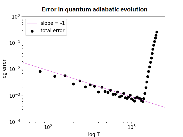
Figure 1: Error scaling of DAS. The example is $H_{i}=-\sum_{i}X_{i},H_{f}=-\sum_{i}(Z_{i}+Z_{i}Z_{i+1})$ on $N=8$ sites without periodic boundary conditions. The initial state is the ground state of $H_{i}$. The discretization number is fixed at $M=2000$. The figures illustrate how $\epsilon^{\prime}_{\text{tot}},\epsilon^{\prime}_{\text{adb}}$ and $\epsilon_{\text{tro}}$ scale with parameter $T$ ranging from $[M/50,M]$ evenly. Each point is a complete run of DAS and there are 50 of them in one line. The vertical axis is shown on a $\log_{10}$ scale. The first figure is only about $\epsilon^{\prime}_{\text{tot}}$, the second figure is a combination of $\epsilon^{\prime}_{\text{adb}}$ and $\epsilon_{\text{tro}}$. As to $\epsilon^{\prime}_{\text{adb}}$, the overall scaling of $\mathcal{O}(T^{-1})$ indicates the correctness of prediction by adiabatic theorem. Note that the Trotter error remains small when $T,M$ are comparable to each other. $\epsilon^{\prime}_{\text{tot}}$ is close to the summation of $\epsilon^{\prime}_{\text{adb}}$ and $\epsilon_{\text{tro}}$. The overall scaling is similar to that of $\epsilon^{\prime}_{\text{adb}}$, while after a turning point the error grows rapidly, and the curve matches with that of $\epsilon_{\text{tro}}$. The turning point is the place where the minimal error is reached. Approximately it’s $0.75M$.

We focus on the Trotter error in DAS,

$$\epsilon_{\text{tro}}\equiv\|A_{d}P_{i}A^{\dagger}_{d}-A_{t}P_{i}A^{\dagger}_{t}\|\leq\|A_{d}-A_{t}\|$$ (29)

which has previously been bounded in terms of operator norm : $\|A_{d}-A_{t}\|=\mathcal{O}(T^{2}/M)$ barends2016digitized . However, as indicated by the adiabatic theorem, all we need to control is the fidelity error, and by building on the techniques in Corollary 1 we will demonstrate that $\epsilon_{\text{tro}}$ has a tighter upper bound that differs from $\|A_{d}-A_{t}\|$. We associate a time-evolving effective Hamiltonian $\widetilde{H}(s)$ with $U^{t}(s)$,

$$\widetilde{H}(s)\equiv i\log(U^{t}(s))/\bar{\delta t}$$ (30)

Notice that at the beginning point $s=0$ and end point $s=1$, $\widetilde{H}(s)$ is the same as $H_{i}$ and $H_{f}$. So the adiabatic evolution under $\widetilde{H}(s)$ can also transform $|\psi_{i}\rangle$ to $|\psi_{f}\rangle$. Naturally the total error should also be quantified with adiabatic theorem.

$$\epsilon^{\prime}_{\text{tot}}\equiv\|P_{f}-A_{t}P_{i}A^{\dagger}_{t}\|$$ (31)

Again, we require that the error caused by discretization is negligible:

$$\epsilon_{\text{tot}}\equiv\|P_{f}-\widetilde{A}(T)P_{i}\widetilde{A}^{\dagger}(T)\|$$

$$\widetilde{A}(T)\equiv\exp_{\mathcal{T}}\left(-iT\int_{0}^{1}\widetilde{H}(s)ds\right)$$

$$\widetilde{\epsilon}_{\text{dis}}\equiv|\epsilon^{\prime}_{\text{tot}}-\epsilon_{\text{tot}}|\ll\epsilon_{\text{tot}}$$

Here $\epsilon_{\text{tot}}$ is the adiabatic error of evolution under $\widetilde{H}(s)$, which is also the continuous limit of $\epsilon^{\prime}_{\text{tot}}$. Using the adiabatic theorem we have:

$$\epsilon_{\text{tot}}\leq\mathcal{G}(T,\widetilde{H})$$ (32)

Combining with Lemma 2, Lemma 4 and the triangle inequality $\epsilon_{\text{tro}}\leq\epsilon^{\prime}_{\text{adb}}+\epsilon^{\prime}_{\text{tot}}$, we prove the following proposition in Appendix F.

Proposition 1.

Consider a digital adiabatic evolution with initial Hamiltonian $H_{i}$, final Hamiltonian $H_{f}$, total evolution time $T$, and discretization number $M$. If the discretization error is negligible comparing to the continuous limit then

$$\epsilon_{dis}\ll\epsilon_{adb},\quad\widetilde{\epsilon}_{dis}\ll\epsilon_{tot}$$ (33)

then the Trotter error has upper bound:

$$\epsilon_{\text{tro}}=\mathcal{O}(\mathcal{G}(T,H)+\mathcal{G}(T,\widetilde{H}))$$ (34)

with $\mathcal{G}$ introduced in Lemma 4. Define:

$$C_{0}\equiv\|H_{i}\|,\quad C_{1}\equiv\|[H_{i},H_{f}]\|$$

$$D\equiv\|H_{i}-H_{f}\|$$

when $D/\lambda\gg 1$, where $\lambda$ is the lower bound of spectral gap during adiabatic evolution under $H(s)$ and $\widetilde{H}(s)$, and $(C_{0}+3D/2)T<M/4$, we obtain:

$$\epsilon_{\text{tro}}=\mathcal{O}\left(\frac{D^{2}}{T\lambda^{3}}\right)+\mathcal{O}\left(\frac{C_{1}^{2}T}{M^{2}\lambda^{3}}\right)$$ (35)

From Proposition 35 we already derive a result different from $\|A_{d}-A_{t}\|$. Numerical results (see Fig. 1) seem to indicate that $\epsilon_{\text{tro}}$ is close to $\epsilon^{\prime}_{\text{tot}}-\epsilon^{\prime}_{\text{adb}}$, which means this result can be further improved. Also this result only works for $T/M=\mathcal{O}(N^{-1})$.

Though taken for granted in most works, the criterion for Eq : (33) to hold is critical to the error analysis. This question has its independent interest. The discretized adiabatic evolution has been the subject of some analysis ambainis2004elementary , but we believe the result can be intrinsically improved and thus leave it for future work.

III Applications

III.1 Quantum Phase Estimation

The QPE algorithm constructs a quantum circuit to detect the phase $\theta$ of a unitary operator: $U|\psi\rangle=e^{i\theta}|\psi\rangle$. For an exact QPE algorithm, the measurement outcome is the integer $a$ closest to $2^{l}\theta$, where $l$ is the size of the first register. Since it’s unlikely for $2^{l}\theta$ to be an integer, there is an inherent error $\xi=\mathcal{O}(2^{-l})$ in this algorithm. The probability of measuring the value closest to the true $\theta$ is at least $4/\pi^{2}$ nielsen2002quantum .

The influence of the Trotter error comes from two aspects. Again we regard the Trotterized evolution operator as an exact evolution operator under the effective Hamiltonian $\widetilde{H}$. This effective Hamiltonian has an eigenstate $|\widetilde{\psi}\rangle$, which is very close to initial eigenstate $|\psi\rangle$ : $|\psi\rangle=\sqrt{1-p}|\widetilde{\psi}\rangle+\sqrt{p}|\widetilde{\psi}^{\perp}\rangle$. As a result, the final phase detected should be $\widetilde{\theta}$ and the success rate should be decreased by a factor of $(1-p)$. However, since usually $p$ is much smaller comparing to 1, this change in success rate is almost negligible.

More importantly, the Trotter error in phase $\delta\theta=|\widetilde{\theta}-\theta|$ should satisfy $\delta\theta<\xi$, otherwise the phase error caused by Trotterization will be detected. This relation gives us a constraint on the Trotter error:

$$|\widetilde{E}-E|t\leq\xi$$ (36)

In QPE, $\theta$ should be set to be close to 1 to avoid wasting the accuracy provided by the first register, thus $t=\mathcal{O}(1/|E|)$. However, we can only guess about $E$ before the algorithm. Here we use $t_{0}$ to denote an appropriate choice of time scale in $U$. Thus

$$L=\mathcal{O}\left(\frac{t_{0}}{\delta t}\right)$$ (37)

where $L$ is the Trotterization number.

The following result follows from Lemma 19.

Corollary 2.

Suppose there’s a quantum circuit performing QPE, the size of the first register is $l$ thus the inherent error is $\xi=\mathcal{O}(2^{-l})$. The unitary operator is $U=e^{-iHt_{0}}$ where $H$satisfies one of the conditions from Lemma 19 in the previous section. To guarantee that the Trotter error in phase is smaller than the inherent error $\xi$, we have:

$$\delta t=\mathcal{O}\left(\frac{1}{N}\sqrt{\frac{\xi}{t_{0}}}\min\{1,\lambda\}\right)$$ (38)

$$L=\mathcal{O}\left(N\sqrt{\frac{t_{0}^{3}}{\xi}}\max\left\{1,\frac{1}{\lambda}\right\}\right)$$ (39)

$$\text{Circuit Depth}=\mathcal{O}\left(\sqrt{\frac{N^{3}t_{0}^{3}}{\xi^{3}}}\max\left\{1,\frac{1}{\lambda}\right\}\right)$$ (40)

$\lambda$ is the lower bound of spectral gap between initial state $|\psi\rangle$ and its neighboring eigenstates.

As a comparison, in general case with $|\widetilde{E}-E|=\mathcal{O}(N\delta t)$, the final circuit depth is $\mathcal{O}(N^{2}t^{2}_{0}/\xi^{2})$.

III.2 Optimizing Digital Adiabatic Simulation

Although a better upper bound of $\epsilon_{\text{tro}}$ has been derived in Proposition 35, it is really $\epsilon^{\prime}_{\text{tot}}$ rather than $\epsilon_{\text{tro}}$ that is the most relevant quantity, for it doesn’t matter whether the error originates from numerical procedure or the finite size of $T$. Motivated by this, here we elaborate on a different question: given a DAS task with $H_{i}$, $H_{f}$ and $|\psi_{i}\rangle$ specified, and a quantum computer with fixed circuit depth $M$, find the optimal $T$ to minimize the estimated total error $\epsilon^{\prime}_{\text{tot}}$.

There exists a trade-off between Trotter error and adiabatic error: on one hand, $T$ can’t be too small as the adiabatic error is inversely proportional to $T$; on the other hand, the error caused by Trotterization increases with $T$ (for a fixed depth $M$). The trade-off is balanced when the two errors are of the same magnitude. We use $T_{c}$ to denote the balanced point, which is exactly the turning point in Fig. 1, if our estimation of $\epsilon_{\text{tot}}$ is accurate enough. The value of $T_{c}$ depends on the estimation of $\epsilon^{\prime}_{\text{tot}}$. In Proposition 35 we have derived an upper bound for $\epsilon^{\prime}_{\text{tot}}$ and denote it with the function $\mathcal{G}(T,\widetilde{H})$. The critical value of $T_{c}$ and the optimal error are defined by

$$\epsilon_{\text{opt}}\equiv\inf_{T}\mathcal{G}(T,\widetilde{H}),\quad T_{c}\equiv\arg\min\mathcal{G}(T,\widetilde{H}).$$ (41)

The next Corollary indicates that $T_{c}$ is proportional to $M$ and their optimal ratio determines the gate complexity of DAS. The result follows from Proposition 35.

Corollary 3 (Optimal choice of $T$).

In the setting of Proposition 35, we intend to perform a digital adiabatic evolution on a quantum device with circuit depth $M$. If $(8C_{0}+12D)D\leq 3C_{1}$, then the upper bound of $\epsilon^{\prime}_{\text{tot}}$ reaches its minimal value at:

$$T_{c}=\frac{2MD}{3C_{1}}$$ (42)

Accordingly,

$$\epsilon_{\text{opt}}=\mathcal{O}\left(\frac{DC_{1}}{M\lambda^{3}}\right)$$ (43)

Alternatively, to achieve an error $\epsilon$ we can keep the ratio $T_{c}/M$ fixed and take the depth of quantum circuit $M$ to be:

$$\text{Circuit Depth}=\mathcal{O}\left(\frac{NDC_{1}}{\lambda^{3}\epsilon}\right)$$ (44)

$N$ is the width of quantum circuit and $\lambda$ is the lower bound of spectral gap.

However, the $T_{c}$ derived still deviates a lot from the turning point in Fig. 1, because our estimation of $\epsilon^{\prime}_{\text{tot}}$ is much larger than the actual value. A tighter bound for $\epsilon^{\prime}_{\text{tot}}$ would lead to a more accurate estimate of $T_{c}$. Additional factors may contribute to the location of the turning point; for example, if the spectral gap of $\widetilde{H}(s)$ closes as $\delta t$ gets larger, the application of the adiabatic theorem will eventually fail.

IV Conclusion $\&$ Outlook

Our main contribution is the observation that refined estimation of Trotter error can be established from effective Hamiltonian $\widetilde{H}$. When the initial state is an eigenstate, we first relate the fidelity error and phase error to the spectrum analysis of $\widetilde{H}$, and find that during evolution, most error accumulates in the phase. Further, if the leading perturbation term of $\widetilde{H}$ vanishes in the eigenbasis of $H$, the Trotter error in energy is reduced from $\mathcal{O}(\delta t)$ to $\mathcal{O}(\delta t^{2})$, which results in improvement of QPE. We remark that the improvement in Trotter step size with phase estimation error $\epsilon$ from $\epsilon$ to $\epsilon^{1/2}$ can be compared to the step size of $\epsilon^{1/2}$ that is obtained from the use of a second-order product formula approximation. Similar results apply to other QPE methods such as robust phase estimation russo2020evaluating (see Appendix G), as long as the Trotterized unitary operator is used. Finally, we show that the spectral analysis method is particularly suitable to analyzing Trotter error in DAS, and we demonstrate how consideration of the various types of error leads to an optimal time parameter $T_{c}$ for DAS when the circuit depth of the quantum circuit is fixed.

There are many targets to pursuit in future work. Here we have only studied Trotter error for the 1st order product formula, and it will be interesting to see whether similar properties exist for higher-order product formulas. One may also seek examples of $f\ll\Delta^{2}$ in time-dependent Hamiltonian situation, in which the initial state is the eigenstate of the initial Hamiltonian, generalizing our results for DAS. Third, numerically the Trotter error in DAS is more close to $\epsilon^{\prime}_{\text{tot}}-\epsilon^{\prime}_{\text{adb}}$ rather than the summation of them, we believe with detail analysis this improvement can be achieved. The forth point is the criterion for the time step scale $T/M$ in DAS that keeps the error caused by discretization negligible. Finally, we would like to try the effective Hamiltonian idea in other quantum simulation algorithms campbell2019random ; low2019hamiltonian ; low2017optimal ; berry2015simulating .

V Acknowledgement

We thank Rolando Somma and Burak Şahinoğlu for helpful discussions. This material is based upon work supported by the U.S. Department of Energy, Office of Science, National Quantum Information Science Research Centers, Quantum Systems Accelerator (QSA).

.1 Appendix A : Proof of Eq : (7)

First we will quantify the region for $f$ and $\theta$ in Eq : (2). We know that $f\in[0,1]$ by definition. As to $\theta$, consider the inner product:

$$\langle\psi|U^{\dagger}(t)T(\delta t)^{L}|\psi\rangle=1+\langle\psi|U^{\dagger}(t)\hat{\Delta}|\psi\rangle$$

Since $\Delta\equiv\|T(\delta t)^{L}-U(t)\|\leq 1/\sqrt{2}$:

$$|\sin\theta|\leq|\langle\psi|U^{\dagger}(t)\hat{\Delta}|\psi\rangle|\leq\Delta\leq 1/\sqrt{2}.$$

Thus $|\theta|\in[-\pi/4,\pi/4]$. In this region, $\theta$ satisfies:

$$1-\frac{\theta^{2}}{2}\leq\cos\theta\leq 1-\frac{\theta^{2}}{4}$$

Similarly,

$$1-f\leq\sqrt{1-f}\leq 1-\frac{f}{2}$$

The Euclidean distance between two evolved states $\mathcal{E}=\|T(\delta t)^{L}|\psi\rangle-U(t)|\psi\rangle\|_{2}$ can be exactly represented with $f$ and $\theta$.

$$\mathcal{E}^{2}=2-2\sqrt{1-f}\cos\theta$$ (45)

From above estimation, we can quantify the upper/lower bound of $\mathcal{E}$ in terms of $f$ and $\theta$:

$$2-2\sqrt{1-f}\cos\theta\geq 2-2(1-\frac{f}{2})(1-\frac{\theta^{2}}{4})\geq f+\frac{\theta^{2}}{4}$$

$$2-2\sqrt{1-f}\cos\theta\leq 2-2(1-f)(1-\frac{\theta^{2}}{2})\leq 2f+\theta^{2}$$

Combine them together:

$$f+\frac{\theta^{2}}{4}\leq\mathcal{E}^{2}\leq 2f+\theta^{2}$$

Appendix A A Appendix B : Proof of Lemma 2

Here we exhibit how to compare the spectrum and eigenstates of effective Hamiltonian $\{\widetilde{E}_{k},|\widetilde{\psi}_{k}\rangle\}$ with that of original Hamiltonian $\{E_{k},|\psi_{k}\rangle\}$ rigorously. The method has already been established in [22]. Magnus expansion sets up connection between two types of exponential operators:

$$\exp_{\mathcal{T}}\left[-i\int_{0}^{t}E(\tau)d\tau\right]=\exp(-iX),\quad-iX=\sum_{j}\Omega_{j}$$

$$\Omega_{j}=\frac{1}{j^{2}}\sum_{\sigma\in S_{j}}\frac{(-1)^{d}(-i)^{j}}{C^{d}_{j-1}}\cdot\int_{0}^{t}dt_{1}\cdots\int_{0}^{t_{n-1}}dt_{n}[E(t_{1}),\cdots,[E(t_{n-1}),E(t_{n})],\cdots]$$

where $S_{j}$ is permutation group and $d$ is a constant related to a permutation. This infinite series $\{\Omega_{j}\}$ is called Magnus expansion. It has been proved that:

$$\|\widetilde{H}-H\|\leq\frac{\alpha\delta t}{2}+\delta t^{2}(\beta+32\alpha\|H\|)$$

With parameters defined in Lemma 2. There are lots of constrains for $\delta t$ in the derivation, we summarize these constraints by setting $\delta t=\mathcal{O}(N^{-1})$. As to $\|\widetilde{H}^{\prime}\|$, previous results show:

$$\widetilde{H}=H-\frac{i}{2}\hat{\alpha}\delta t+\frac{1}{\delta t}\int_{0}^{\delta t}dx\hat{\beta}(x)+\frac{1}{\delta t}\sum_{n=2}\Omega_{n}(\delta t)$$

$$\hat{\alpha}=\sum_{l>m}[H_{l},H_{m}],\quad\|\hat{\beta}(x)\|\leq x^{2}\beta$$

$$\|\Omega_{n}\|\leq\sum_{\sigma}\int\cdots\int dt_{1}\cdots dt_{n}\mathcal{C}_{n}$$

$$\mathcal{C}_{n}\leq 2^{n}(\|H\|+\alpha\delta t+\beta\delta t^{2})^{n-1}(\alpha\delta t+\beta\delta t^{2})$$

When we upper bound the derivatives, we separate the above expression into three parts and consider the worst case: (we write $\delta t$ as $t$ temporarily for abbreviation)

$$\|\left(\frac{1}{t}\int_{0}^{t}\hat{\beta}(x)dx\right)^{\prime}\|\leq\frac{1}{t}\|\hat{\beta}(t)\|+\frac{1}{t^{2}}\int_{0}^{t}\|\hat{\beta}(x)\|dx\leq\frac{4}{3}\beta t$$

Next we will prove $\|\sum_{n=2}\Omega^{\prime}_{n}(t)\|\leq\omega t^{2}$ to directly use the above scenario.

$$\|\sum_{n=2}\Omega^{\prime}(t)\| \leq\sum_{n=2}n!\frac{t^{n-1}}{(n-1)!}\mathcal{C}_{n}$$

$$\leq\sum_{n=2}nt^{n-1}2^{n}(\|H\|+\alpha t+\beta t^{2})^{n-1}(\alpha t+\beta t^{2})$$

$$=2t(\alpha+\beta t)\sum_{n=2}n(2\|H\|t+2\alpha t^{2}+2\beta t^{3})^{n-1}$$

$$=2t(\alpha+\beta t)g(2\|H\|t+2\alpha t^{2}+2\beta t^{3})$$

where $g(y)=(y^{2}/(1-y))^{\prime}<4y+4y^{2}<8y$ when $y<1/2$. Thus:

$$\omega=128\alpha\|H\|$$

Replace $t$ with $\delta t$. Finally:

$$\|\widetilde{H}^{\prime}(\delta t)\|\leq\frac{\alpha}{2}+\frac{4}{3}(\beta+128\alpha\|H\|)\delta t$$

A.1 Appendix C : Proof of Cororllary 1

This result is a special case of Theorem 1. Here we prove it in a more direct way. Calculate the inner product between $U(t)|\psi_{k}\rangle$ and $T(\delta t)^{L}|\psi_{k}\rangle$ using spectral decomposition $\widetilde{H}=\sum_{j}\widetilde{E}_{j}\widetilde{P}_{j}$:

$$\sqrt{1-f}e^{i\theta} =\langle\psi_{k}|U^{\dagger}(t)T(\delta t)^{L}|\psi_{k}\rangle$$

$$=\sum_{j}e^{i(E_{k}-\widetilde{E}_{j})t}|\langle\psi_{k}|\widetilde{\psi}_{j}\rangle|^{2}$$

$$=e^{i(E_{k}-\widetilde{E}_{k})t}|\langle\psi_{k}|\widetilde{\psi}_{k}\rangle|^{2}+\sum_{j\neq k}e^{i(E_{k}-\widetilde{E}_{j})t}|\langle\psi_{k}|\widetilde{\psi}_{j}\rangle|^{2}$$

$$=e^{i(E_{k}-\widetilde{E}_{k})t}\left[|\langle\psi_{k}|\widetilde{\psi}_{k}\rangle|^{2}+\sum_{j\neq k}e^{i(\widetilde{E}_{k}-\widetilde{E}_{j})t}|\langle\psi_{k}|\widetilde{\psi}_{j}\rangle|^{2}\right]$$

Define $\varepsilon$ and $\eta$ as:

$$\varepsilon=1-|\langle\psi_{k}|\widetilde{\psi}_{k}\rangle|^{2},\quad\eta=\sum_{j\neq k}e^{i(\widetilde{E}_{k}-\widetilde{E}_{j})t}|\langle\psi_{k}|\widetilde{\psi}_{j}\rangle|^{2}$$

Then:

$$1-f=|1-\varepsilon+\eta|^{2},\quad\theta=(E_{k}-\widetilde{E}_{k})t+\text{Arg}(1-\varepsilon+\eta)$$

The complex number $\eta$ is upper bounded by $|\eta|\leq\varepsilon$ and the equality is satisfied when all the phases $(\widetilde{E}_{j}-\widetilde{E}_{k})t$ differ by $2\pi j$, hence:

$$f=\mathcal{O}(1-|\langle\psi_{k}|\widetilde{\psi}_{k}\rangle|^{2}),\quad\theta=\mathcal{O}(|\widetilde{E}_{k}-E_{k}|t)$$

Combine with Lemma 2:

$$f=\mathcal{O}\left(\frac{h^{2}\delta t^{2}}{\lambda^{2}}\right),\quad|\theta|=\mathcal{O}(Lh\delta t^{2})$$

Of course, $f=\theta=0$ when $L=0$. However, in this upper bound $f$ is irrelevant to $L$. To fix this, notice we have another upper bound for $f$ from Eq : (7):

$$f\leq\mathcal{E}^{2}\leq\Delta^{2}=\mathcal{O}(L^{2}h^{2}\delta t^{4})$$

Appendix B B Appendix D : Proof of Eq : (13) and Theorem 1

Consider the norm distance between two projectors $\delta p=\|P_{x}-P_{y}\|,P_{x}=|x\rangle\langle x|,P_{y}=|y\rangle\langle y|$, one observation is that this matrix is normal, hence its norm is the largest value of absolute eigenvalues of the following matrix:

$$|y\rangle=a|x\rangle+b|x^{\perp}\rangle,\quad\Delta P=\begin{bmatrix}1-a^{2}&-ab\\ -ab&-b^{2}\end{bmatrix}$$

Although $\Delta P$ is only the representation of projector difference in a subspace spanned by $\{|x\rangle,|y\rangle\}$, other dimensions won’t effect the spectrum of it. The parameters $a,b$ can be set as non-negative real numbers for there are two degrees of freedom on the phases of $|y\rangle$ and $|x^{\perp}\rangle$. Also $a^{2}$ is the fidelity between two states.

Solve this matrix, the largest absolute value of $\Delta P$ is:

$$\delta p=b=\sqrt{1-|\langle x|y\rangle|^{2}}$$

We also also extend this result to multi-state projectors. Suppose we have two projectors $P_{A}$ and $P_{B}$ that each corresponds to an $m$-dimensional subspace. $A$,$B$ are the invariant spaces of the two projectors. To make the problem meaningful, they should be close to each other in the sense that $\|P_{A}-P_{B}\|<1$. In another word, $A$ and $B$ share $m-1$ dimensions. Then we can re-choose two sets of basis in $A$ and $B$ such that only one element is different. Then the problem is reduced to the previous one. Based on this observation:

$$\min_{|\phi_{a}\rangle\in\mathcal{H}_{A}}\text{tr}(P_{B}|\phi_{a}\rangle\langle\phi_{a}|)=1-\|P_{A}-P_{B}\|^{2}$$

Similar result can be extended to mixed state, since the extreme status corresponds to pure state:

$$\min_{\rho_{a}\in\mathcal{H}_{A}}\text{tr}(P_{B}\rho_{a})=1-\|P_{A}-P_{B}\|^{2}$$ (46)

In Theorem 1, we have an original projector $P$ that is composed of $m$ eigenstate projectors, and an “effective” projector $\widetilde{P}$ which is very close to $P$. Their norm distance has been well-quantified. Write:

$$\delta p\equiv\|\widetilde{P}-P\|$$

Our initial state $\rho$ is a mixed state inside the space of $P$, which means $\text{tr}(\rho P)=1$. In Eq : (46) we have proved that:

$$\text{tr}(\rho\widetilde{P})\geq 1-\delta p^{2}$$

Now we want to quantify the leakage rate:

$$1-\text{tr}(\widetilde{U}\rho\widetilde{U}^{\dagger}P)=1-\text{tr}(\rho\widetilde{U}^{\dagger}P\widetilde{U})$$

where $\widetilde{U}$ is the Trotterized evolution operator. Easy to see that $[\widetilde{U},\widetilde{P}]=0$. Therefore:

$$\|\widetilde{P}-\widetilde{U}^{\dagger}P\widetilde{U}\|=\|\widetilde{P}-P\|=\delta p$$

$$\widetilde{U}^{\dagger}P\widetilde{U}=P+(\widetilde{P}-P)+(\widetilde{U}^{\dagger}P\widetilde{U}-\widetilde{P})$$

$$\|\widetilde{U}^{\dagger}P\widetilde{U}-P\|\leq 2\delta p$$

Use the same argument in Eq : (46) we derive:

$$\text{tr}(\rho\widetilde{U}^{\dagger}P\widetilde{U})\geq 1-4\delta p^{2}$$

$$1-\text{tr}(\rho\widetilde{U}^{\dagger}P\widetilde{U})=\mathcal{O}(\delta p^{2})$$

The leakage rate has order $\mathcal{O}(\delta p^{2})$.

Appendix C C Appendix E : Proof of Lemma 19

Define $H(s)$ as:

$$H(s)\equiv H+sV,\quad V\equiv\frac{i}{2}\sum_{l>m}[H_{l},H_{m}]$$

with eigenstates and eigenvalues:

$$H(s)|\psi(s)\rangle=E(s)|\psi(s)\rangle$$

The actual effective Hamiltonian satisfies $\widetilde{H}=H(\delta t)+V_{2}$. Use the method in Lemma 2 we can prove $\|V_{2}\|=\mathcal{O}(\delta t^{2}(\beta+32\alpha\|H\|))$. We focus on the error in energy caused by $H(s)$ first. Lemma 19 states that $\langle\psi(0)|V|\psi(0)\rangle=0$. To exploit this condition, define fidelity distance $f(s)$ from the following equation:

$$|\psi(s)\rangle=\sqrt{1-f(s)}|\psi(0)\rangle+\sqrt{f(s)}|\psi(0)^{\perp}\rangle$$

We don’t need $e^{i\theta(s)}$ as there’s a degree of freedom on the phase of $|\psi(s)\rangle$. Use the method in Corollary 1 we have:

$$1-|\langle\psi(0)|\psi(s)\rangle|^{2}=f(s)=\|P(s)-P(0)\|^{2}$$

$$\|P(s)-P(0)\|\leq s\max_{x\in[0,s]}\|P^{\prime}(x)\|,\max_{x\in[0,s]}\|P^{\prime}(x)\|\leq\frac{\|V\|}{\lambda}$$

Hence, $f(s)\leq\frac{\|V\|^{2}s^{2}}{\lambda^{2}}$. Since $E(s)=\langle\psi(s)|H(s)|\psi(s)\rangle$ and $\langle\psi(0)|V|\psi(0)\rangle=0$:

$$E(s)-E(0)= \langle\psi(s)|H(s)|\psi(s)\rangle-\langle\psi(0)|H|\psi(0)\rangle$$

$$= f(s)(\langle\psi(0)^{\perp}|H|\psi(0)^{\perp}\rangle-\langle\psi(0)|H|\psi(0)\rangle)+f(s)s\langle\psi(0)^{\perp}|V|\psi(0)^{\perp}\rangle$$

$$+s\sqrt{(1-f(s))f(s)}(\langle\psi(0)|V|\psi(0)^{\perp}\rangle+c.c)$$

Here we use the following argument for upper bound:

$$|\phi\rangle=\frac{1}{\sqrt{2}}(|\phi\rangle+|\psi^{\perp}\rangle)$$

$$\langle\phi|V|\phi\rangle=\frac{1}{2}(\langle\psi|V|\psi\rangle+\langle\psi^{\perp}|V|\psi^{\perp}\rangle+\langle\psi|V|\psi^{\perp}\rangle+c.c)$$

$$\langle\psi|V|\psi^{\perp}\rangle+c.c\leq 2\|V\|$$

Finally:

$$|E(s)-E(0)|\leq\frac{\|V\|^{2}\cdot\|H\|s^{2}}{\lambda^{2}}+\frac{2\|V\|^{2}s^{2}}{\lambda}+\frac{\|V\|^{3}s^{3}}{\lambda^{2}}$$

When $\|V\|s<\lambda$ and $\|H\|>2\lambda$, only the first term remains. Thus:

$$|E(\delta t)-E(0)|=\mathcal{O}\left(\frac{\|V\|^{2}\cdot\|H\|\delta t^{2}}{\lambda^{2}}\right)$$ (47)

Quantify the error caused by $V_{2}$ with Weyl’s inequality:

$$|\widetilde{E}-E(0)| \leq|\widetilde{E}-E(\delta t)|+|E(\delta t)-E(0)|$$

$$=\mathcal{O}(\delta t^{2}(\beta+32\alpha\|H\|))+\mathcal{O}\left(\frac{\|V\|^{2}\cdot\|H\|\delta t^{2}}{\lambda^{2}}\right)$$

$$=\mathcal{O}\left(N^{2}\delta t^{2}\max\left\{1,\frac{1}{\lambda^{2}}\right\}\right)$$

Appendix D D Appendix F : Proof of Proposition 35 and Corollary 3

The content in this Appendix is nothing more than combining Lemma 2 with Lemma 4. To quantify $\mathcal{G}(T,\widetilde{H})$, our target is the derivative of $\widetilde{H}(s)$ defined as:

$$\widetilde{H}(s)\equiv i\log\left(\exp(-it(1-s)H_{i})\exp(-itsH_{f})\right)/t$$

We use $t$ to denote $\delta t$ for simplicity in this Appendix. $\widetilde{H}$ satisfies:

$$e^{-it\widetilde{H}(s)}=e^{-itH_{i}}\cdot\left(e^{istH_{i}}e^{-istH_{f}}\right)=e^{-itH_{i}}e^{-itG(s)}$$

We separate the calculation of $\widetilde{H}$ into two parts. In the first part we take derivative with respect to $t$, and represent $\widetilde{H}$ with $H_{i}$ and $G(s)$; next we calculate $G(s)$ by taking derivatives with respect to $s$ instead. The procedure is similar to that of Appendix B. The following special functions are used in the estimation:

$$\mathcal{F}_{0}(x)=\sum_{j=0}^{\infty}x^{j}=\frac{1}{1-x}$$

$$\mathcal{F}_{1}(x)=\sum_{j=1}^{\infty}\frac{1}{j}x^{j-1}=-\ln(1-x)/x$$

$$\mathcal{F}_{2}(x)=\sum_{j=2}^{\infty}\frac{1}{j^{2}}x^{j}=\int_{0}^{x}-\ln(1-x^{\prime})dx^{\prime}$$

They have the following upper bounds when $0\leq x\leq 1/2$:

$$\mathcal{F}_{0}\leq 1+2x,\quad\mathcal{F}_{1}\leq 1+x,\quad\mathcal{F}_{2}\leq\frac{x^{2}}{2}(1+x)$$

We express $\widetilde{H}$ in terms of $G$ first. Under the setting of Magnus expansion:

$$-it\widetilde{H}(s)=\sum_{j=1}^{\infty}\Omega_{j}(s,t),\quad E(s,t)=-ie^{-itH_{i}}(H_{i}+G(s,t))e^{itH_{i}}$$

$$\Omega_{j}(s,t)=\frac{1}{j^{2}}\sum_{\sigma\in S_{j}}\frac{(-1)^{d}}{C^{d}_{j-1}}\int_{0}^{t}dt_{1}\cdots\int_{0}^{t_{j-1}}dt_{j}[E(t_{1}),\cdots[E(t_{j-1}),E(t_{j})]]$$

$d$ is a constant relevant to permutation $\sigma$. As to $\widetilde{H}^{\prime}(s)$, the integrand in $\Omega^{\prime}_{j}(s)$ becomes summation over $j$ different commutators; while for $\widetilde{H}^{\prime\prime}(s)$, the integrand of $\Omega_{j}^{\prime\prime}(s)$ contains $j(j-1)$ pairs of $E^{\prime}$ or $j$ $E^{\prime\prime}$. Thus:

$$\|\widetilde{H}^{\prime}(s)\|\leq\|G^{\prime}\|\cdot\mathcal{F}_{1}\left(2(\|H_{i}+G\|)t\right)$$

$$\|\widetilde{H}^{\prime\prime}(s)\|\leq\|G^{\prime\prime}\|\cdot\mathcal{F}_{1}\left(2(\|H_{i}+G\|)t\right)+2\|G^{\prime}\|^{2}t\cdot\mathcal{F}_{0}(2\|H+G\|t)$$

The next step is to represent $G(s,t)$ with $H_{i}$ and $H_{f}$, and we consider $s$ as variable instead.

$$\frac{d}{ds}e^{-itG(s,t)}=\widetilde{E}(s,t)e^{-itG(s,t)},\quad\widetilde{E}(s,t)=e^{istH_{i}}(itH_{i}-itH_{f})e^{-istH_{i}}$$

$$G(s,t)=its(H_{i}-H_{f})+t^{2}\int_{0}^{s}ds^{\prime}\int_{0}^{s^{\prime}}ds^{\prime\prime}e^{its^{\prime\prime}H_{i}}[H_{i},H_{f}]e^{-its^{\prime\prime}H_{i}}+\sum_{j=2}^{\infty}\widetilde{\Omega}_{j}(s,t)$$

$$\widetilde{\Omega}_{j}(s,t)=\frac{1}{j^{2}}\sum_{\sigma\in S_{j}}\frac{(-1)^{d}}{C^{d}_{j-1}}\int_{0}^{s}ds_{1}\cdots\int_{0}^{s_{j-1}}ds_{j}[E(s_{1}),\cdots,[E(s_{j-1}),E(s_{j})]]$$

To abbreviate the result, define:

$$C_{0}\equiv\|H_{i}\|,\quad C_{1}\equiv\|[H_{i},H_{f}]\|,\quad C_{2}\equiv\|[H_{i},[H_{i},H_{f}]]\|,\quad D\equiv\|H_{i}-H_{f}\|$$

Notice that we treat $\widetilde{\Omega}_{1}(s,t)$ separately to derive a better result. The norm of $G(s,t),G^{\prime}(s,t)$ and $G^{\prime\prime}(s,t)$ can be bounded by:

$$\|G(s,t)\|\leq sD+\frac{1}{2t}\mathcal{F}_{2}(2stD)$$

$$\|\frac{d}{ds}G(s,t)\|\leq D+stC_{1}\mathcal{F}_{1}(2stD)$$

$$\|\frac{d^{2}}{ds^{2}}G(s,t)\|\leq C_{1}t+2C_{1}^{2}s^{2}t^{3}\mathcal{F}_{0}(2stD)+C_{2}st^{2}(\mathcal{F}_{1}(2stD)-1)$$

Combine everything together:

$$\|\widetilde{H}^{\prime}(s)\|\leq[D+C_{1}t(1+2Dt)][1+(2C_{0}+3D)t]$$

$$\|\widetilde{H}^{\prime\prime}(s)\|\leq\left(C_{1}t+4C_{1}^{2}t^{3}+2DC_{2}t^{3}\right)[1+(2C_{0}+3D)t]+2t\left(D+C_{1}t(1+2Dt)\right)^{2}\frac{1}{1-(2C_{0}+3D)t}$$

Here it’s required that $tD<1/4$ and $(\|H_{i}\|+\max\|G(s)\|)t<1/4$.

Put the above results in $\mathcal{G}(T,\widetilde{H})$:

$$\mathcal{G}(T,\widetilde{H}) =\frac{1}{T}\left(\frac{\|\widetilde{H}^{\prime}(0)\|}{\widetilde{\lambda}(0)^{2}}+\frac{\|\widetilde{H}^{\prime}(1)\|}{\widetilde{\lambda}(1)^{2}}\right)+\frac{1}{T}\int_{0}^{1}\frac{\|\widetilde{H}^{\prime\prime}(s)\|}{\widetilde{\lambda}^{2}(s)}+7\frac{\|\widetilde{H}^{\prime}(s)\|^{2}}{\widetilde{\lambda}^{3}(s)}ds$$

$$\leq\frac{2}{T\lambda^{2}}\max\|\widetilde{H}^{\prime}(s)\|+\frac{1}{T\lambda^{2}}\max\|\widetilde{H}^{\prime\prime}(s)\|+\frac{7}{T\lambda^{3}}\max\|\widetilde{H}^{\prime}(s)\|^{2}$$

$\lambda\equiv\inf_{s}\{\widetilde{\lambda}(s)\}$. In this upper bound, $\widetilde{H}^{\prime\prime}(s)$ won’t appear in the leading term. Given $N$ as the size of the system, roughly, the magnitudes of quantities are $t=\mathcal{O}(N^{-1}),D=\mathcal{O}(N),C_{k}=\mathcal{O}(N^{k+1})$. As a result, $\|\widetilde{H}^{\prime}\|=\mathcal{O}(N),\|\widetilde{H}^{\prime\prime}\|=\mathcal{O}(N)$, and the leading term of the upper bound is:

$$\epsilon_{\text{tot}} \leq\mathcal{O}\left(\frac{1}{T\lambda^{3}}\left(D+C_{1}t(1+2Dt)\right)^{2}[1+(2C_{0}+3D)t]^{2}\right)$$

$$=\mathcal{O}\left(\frac{1}{T\lambda^{3}}\left(D+\frac{3C_{1}T}{2M}\right)^{2}\right)$$

The maximal of the above upper bound is reached at:

$$\frac{T_{c}}{M}=\frac{2D}{3C_{1}}$$ (48)

We further requires that $(8C_{0}+12D)D\leq 3C_{1}$ to let $T_{c}$ satisfies $(\|H_{i}\|+\max\|G(s)\|)T<M/4$.

Appendix E E Appendix G : Trotter Error in Robust Phase Estimation

The idea of Robust Phase Estimation is, begin with two quantum states:

$$|\alpha\rangle=\frac{1}{\sqrt{2}}\left(|0\rangle+|1\rangle\right)$$

$$|\beta\rangle=\frac{1}{\sqrt{2}}\left(|0\rangle+i|1\rangle\right)$$

The target is the phase difference $(E_{0}-E_{1})t$. It can be derived from the outcome of two measurements:

$$P_{\alpha}=|\langle\alpha|U(t)|\alpha\rangle|^{2}=\frac{1}{2}(1+\cos((E_{1}-E_{0})t))$$

$$P_{\beta}=|\langle\alpha|U(t)|\beta\rangle|^{2}=\frac{1}{2}(1+\sin((E_{1}-E_{0})t))$$

Thus:

$$\tan((E_{1}-E_{0})t)=\frac{2P_{\beta}-1}{2P_{\alpha}-1}$$

Now let’s consider the Trotterized version:

$$|0\rangle=\sqrt{1-f_{0}}|\widetilde{0}\rangle+\sqrt{f_{0}}|\widetilde{0}^{\perp}\rangle$$

$$|1\rangle=\sqrt{1-f_{1}}|\widetilde{1}\rangle+\sqrt{f_{1}}|\widetilde{1}^{\perp}\rangle$$

$$\widetilde{U}|\widetilde{0}\rangle=e^{-i\widetilde{E}_{0}t}|\widetilde{0}\rangle\quad,\quad\widetilde{U}|\widetilde{1}\rangle=e^{-i\widetilde{E}_{1}t}|\widetilde{1}\rangle$$

From here we have:

$$\langle\alpha|\widetilde{U}(t)|\alpha\rangle=\frac{1}{2}[e^{-i\widetilde{E}_{0}t}+e^{-i\widetilde{E}_{1}t}+2\sqrt{f_{1}}\text{Re}(\langle\widetilde{0}|\widetilde{1}^{\perp}\rangle)e^{-i\widetilde{E}_{0}t}+2\sqrt{f_{0}}\text{Re}(\langle\widetilde{0}^{\perp}|\widetilde{1}\rangle)e^{-i\widetilde{E}_{1}t}]+\mathcal{O}(f)$$

$$\langle\alpha|\widetilde{U}(t)|\beta\rangle=\frac{1}{2}[e^{-i\widetilde{E}_{0}t}+ie^{-i\widetilde{E}_{1}t}+\sqrt{f_{0}}e^{-i\widetilde{E}_{1}t}(i\langle\widetilde{0}^{\perp}|\widetilde{1}\rangle+i\langle\widetilde{1}|\widetilde{0}^{\perp}\rangle)$$

$$+\sqrt{f_{1}}e^{-i\widetilde{E}_{0}t}(i\langle\widetilde{0}|\widetilde{1}^{\perp}\rangle+\langle\widetilde{1}^{\perp}|\widetilde{0}\rangle)]+\mathcal{O}(f)$$

And calculate the new probability:

$$\widetilde{P}_{\alpha}=\frac{1}{2}[1+\cos((\widetilde{E}_{1}-\widetilde{E}_{0})t)]+\mathcal{O}(\sqrt{f})$$

$$\widetilde{P}_{\beta}=\frac{1}{2}[1+\sin((\widetilde{E}_{1}-\widetilde{E}_{0})t)]+\mathcal{O}(\sqrt{f})$$

The final value for phase difference is:

$$\delta\widetilde{\theta} =\arctan\left[\frac{2\widetilde{P}_{\beta}-1}{a\widetilde{P}_{\alpha}-1}\right]$$

$$=\arctan(\tan((\widetilde{E}_{1}-\widetilde{E}_{0})t)+\mathcal{O}(\sqrt{f}))$$

$$=(\widetilde{E}_{1}-\widetilde{E}_{0})t+\frac{\mathcal{O}(\sqrt{f})}{1+|\widetilde{E}_{1}-\widetilde{E}_{0}|^{2}t^{2}}+\cdots$$

$$=\delta\theta+(\widetilde{E}_{1}-E_{1}-\widetilde{E}_{0}+E_{0})t+\mathcal{O}(\sqrt{f})$$

The second equation is only true when $\mathcal{O}(\sqrt{f})\ll[1+\cos((\widetilde{E}_{1}-\widetilde{E}_{0})t)]/2$.

We have proved that the trotter error in fidelity doesn’t grow linearly with $L$. Thus, if $t$ is a constant instead of a small quantity, the effect of $\mathcal{O}(\sqrt{f})$ can be neglected. The final error in energy difference has order:

$$|\delta\widetilde{\theta}-\delta\theta|/t=\mathcal{O}(|\widetilde{E}-E|)$$

References

• [1] Hale F Trotter. On the product of semi-groups of operators. Proceedings of the American Mathematical Society, 10(4):545–551, 1959.
• [2] Masuo Suzuki. Generalized trotter’s formula and systematic approximants of exponential operators and inner derivations with applications to many-body problems. Communications in Mathematical Physics, 51(2):183–190, 1976.
• [3] Seth Lloyd. Universal quantum simulators. Science, pages 1073–1078, 1996.
• [4] Andrew M Childs, Yuan Su, Minh C Tran, Nathan Wiebe, and Shuchen Zhu. A theory of trotter error. arXiv preprint arXiv:1912.08854, 2019.
• [5] Andrew M Childs and Yuan Su. Nearly optimal lattice simulation by product formulas. Physical review letters, 123(5):050503, 2019.
• [6] Earl Campbell. Random compiler for fast hamiltonian simulation. Physical review letters, 123(7):070503, 2019.
• [7] As usual in trotterization, the guideline for the decomposition is that one has a way to implement $e^{itH_{j}}$ efficiently for each $H_{j}$. A sufficient condition for this is for each $H_{j}$ to be a sum of pairwise commuting local terms.
• [8] A Yu Kitaev. Quantum measurements and the abelian stabilizer problem. arXiv preprint quant-ph/9511026, 1995.
• [9] Markus Reiher, Nathan Wiebe, Krysta M Svore, Dave Wecker, and Matthias Troyer. Elucidating reaction mechanisms on quantum computers. Proceedings of the National Academy of Sciences, 114(29):7555–7560, 2017.
• [10] Ian D Kivlichan, Craig Gidney, Dominic W Berry, Nathan Wiebe, Jarrod McClean, Wei Sun, Zhang Jiang, Nicholas Rubin, Austin Fowler, Alán Aspuru-Guzik, et al. Improved fault-tolerant quantum simulation of condensed-phase correlated electrons via trotterization. Quantum, 4:296, 2020.
• [11] Michael A Nielsen and Isaac Chuang. Quantum computation and quantum information, 2002.
• [12] Edward Farhi, Jeffrey Goldstone, Sam Gutmann, Joshua Lapan, Andrew Lundgren, and Daniel Preda. A quantum adiabatic evolution algorithm applied to random instances of an np-complete problem. Science, 292(5516):472–475, 2001.
• [13] Dorit Aharonov, Wim Van Dam, Julia Kempe, Zeph Landau, Seth Lloyd, and Oded Regev. Adiabatic quantum computation is equivalent to standard quantum computation. SIAM review, 50(4):755–787, 2008.
• [14] Tameem Albash and Daniel A Lidar. Adiabatic quantum computation. Reviews of Modern Physics, 90(1):015002, 2018.
• [15] Dorit Aharonov and Amnon Ta-Shma. Adiabatic quantum state generation and statistical zero knowledge. In Proceedings of the thirty-fifth annual ACM symposium on Theory of computing, pages 20–29, 2003.
• [16] Kianna Wan and Isaac Kim. Fast digital methods for adiabatic state preparation. arXiv preprint arXiv:2004.04164, 2020.
• [17] Rami Barends, Alireza Shabani, Lucas Lamata, Julian Kelly, Antonio Mezzacapo, Urtzi Las Heras, Ryan Babbush, Austin G Fowler, Brooks Campbell, Yu Chen, et al. Digitized adiabatic quantum computing with a superconducting circuit. Nature, 534(7606):222–226, 2016.
• [18] Yin Sun, Jun-Yi Zhang, Mark S Byrd, and Lian-Ao Wu. Adiabatic quantum simulation using trotterization. arXiv preprint arXiv:1805.11568, 2018.
• [19] Andris Ambainis and Oded Regev. An elementary proof of the quantum adiabatic theorem. arXiv preprint quant-ph/0411152, 2004.
• [20] Sergio Blanes, Fernando Casas, JA Oteo, and José Ros. The magnus expansion and some of its applications. Physics reports, 470(5-6):151–238, 2009.
• [21] Sabine Jansen, Mary-Beth Ruskai, and Ruedi Seiler. Bounds for the adiabatic approximation with applications to quantum computation. Journal of Mathematical Physics, 48(10):102111, 2007.
• [22] Minh C Tran, Yuan Su, Daniel Carney, and Jacob M Taylor. Faster digital quantum simulation by symmetry protection. arXiv preprint arXiv:2006.16248, 2020.
• [23] Burak Şahinoğlu and Rolando D Somma. Hamiltonian simulation in the low energy subspace. arXiv preprint arXiv:2006.02660, 2020.
• [24] Sergey Bravyi and Barbara Terhal. Complexity of stoquastic frustration-free hamiltonians. Siam journal on computing, 39(4):1462–1485, 2010.
• [25] Sergey Bravyi, Libor Caha, Ramis Movassagh, Daniel Nagaj, and Peter W Shor. Criticality without frustration for quantum spin-1 chains. Physical review letters, 109(20):207202, 2012.
• [26] David Poulin, Angie Qarry, Rolando Somma, and Frank Verstraete. Quantum simulation of time-dependent hamiltonians and the convenient illusion of hilbert space. Physical review letters, 106(17):170501, 2011.
• [27] Dominic W Berry, Andrew M Childs, Yuan Su, Xin Wang, and Nathan Wiebe. Time-dependent hamiltonian simulation with l1 -norm scaling. Quantum, 4:254, 2020.
• [28] Donny Cheung, Peter Høyer, and Nathan Wiebe. Improved error bounds for the adiabatic approximation. Journal of Physics A: Mathematical and Theoretical, 44(41):415302, 2011.
• [29] Lucas T Brady, Christopher L Baldwin, Aniruddha Bapat, Yaroslav Kharkov, and Alexey V Gorshkov. Optimal protocols in quantum annealing and qaoa problems. arXiv preprint arXiv:2003.08952, 2020.
• [30] Guido Pagano, Aniruddha Bapat, Patrick Becker, Katherine S Collins, Arinjoy De, Paul W Hess, Harvey B Kaplan, Antonis Kyprianidis, Wen Lin Tan, Christopher Baldwin, et al. Quantum approximate optimization of the long-range ising model with a trapped-ion quantum simulator. Proceedings of the National Academy of Sciences, 2020.
• [31] Leo Zhou, Sheng-Tao Wang, Soonwon Choi, Hannes Pichler, and Mikhail D Lukin. Quantum approximate optimization algorithm: performance, mechanism, and implementation on near-term devices. arXiv preprint arXiv:1812.01041, 2018.
• [32] AE Russo, KM Rudinger, BCA Morrison, and AD Baczewski. Evaluating energy differences on a quantum computer with robust phase estimation. arXiv preprint arXiv:2007.08697, 2020.
• [33] Guang Hao Low and Isaac L Chuang. Hamiltonian simulation by qubitization. Quantum, 3:163, 2019.
• [34] Guang Hao Low and Isaac L Chuang. Optimal hamiltonian simulation by quantum signal processing. Physical review letters, 118(1):010501, 2017.
• [35] Dominic W Berry, Andrew M Childs, Richard Cleve, Robin Kothari, and Rolando D Somma. Simulating hamiltonian dynamics with a truncated taylor series. Physical review letters, 114(9):090502, 2015.