Estimating the effective reproduction number for heterogeneous models using actual data

Abstract

This document contain the Supplementary Materials for the manuscript entitled "Estimating the effective reproduction number for heterogeneous models using incidence data" by Jorge et al.

Supplementary Material 1
Methodology applied to epidemiological compartment models

Applying the method to epidemiological models

We proceed to illustrate the application of the method developed in this work to compartmental epidemic models. We chose two simple models that are known in literature and two variations of a meta-population model that is used in the main framework and developed in Supplementary Material 2. We seek to show the method step by step, presenting its detailed calculations. All models presented are composed of ordinary differential equations. In the transitions between infected compartments described in these models, $\mathbfcal{V}(t,\tau)$, the the infected compartments $\bm{x}(t,\tau)$ appear with linear dependence. Therefore we can simplify:

$$\dfrac{\partial\overline{\mathcal{V}_{i}}}{\partial u_{j}}=\dfrac{\partial\mathcal{V}_{i}}{\partial x_{j}}=cte\qquad\text{and}\qquad\frac{d}{d\omega}\bm{u}(\omega)=-\frac{\partial{\mathbfcal{V}}}{\partial\bm{x}}\bm{u}(\omega).$$ (1)

In addition, all the parameters of the models in this Supplementary Material are constant, which leads to

$$\bm{\Omega}(t)=\frac{\partial}{\partial\bm{X}}{\mathbfcal{F}}(t)\qquad\text{and}\qquad\overline{\bm{\Gamma}}(\omega)=\bm{\Gamma}(\tau)$$ (2)

SEIR model

The SEIR model is designed by introducing a new exposed $E$ stage of the disease into the SIR model [1]. We can assume that when an individual becomes infected, it must go through a latency period before showing its first symptoms and starting to infect other individuals. This is accomplished by introducing the exposed compartment $E$ and its removal rate $\kappa$. Thus, all individuals who are infected start in the exposed state and, on average, after a $1/\kappa$ latency time are introduced into the $I$ compartment. It is also possible to introduce a factor related to a $\epsilon$ pre-symptomatic infection. This way, individuals can start to infect in the exposed compartment, before presenting symptoms. Thus, this model, considering pre-symptomatic infection, can be written as

$$\frac{dS}{dt} =-\frac{\beta S}{N}\Big{[}I+\epsilon E\Big{]},$$ (3)

$$\frac{dE}{dt} =\frac{\beta S}{N}\Big{[}I+\epsilon E\Big{]}-\kappa E,$$ (4)

$$\frac{dI}{dt} =\kappa E-\gamma I,$$ (5)

$$\frac{dR}{dt} =\gamma I.$$ (6)

Thus, we can sort the infected compartments as $\bm{X}(t)=[E(t),\;I(t)]$. In this way the distributions of the infectious phase are defined as $\bm{x}(t,\tau)=[i_{e}(t,\tau),i_{i}(t,\tau)]$. We get ${\mathbfcal{F}}(t)$ e ${\mathbfcal{V}}(t,\tau)$:

$${\mathbfcal{F}}(t)=\begin{pmatrix}\frac{\beta S}{N}\big{[}I+\epsilon E\big{]}\\[4.30554pt] 0\end{pmatrix},\qquad{\mathbfcal{V}}(t,\tau)=\begin{pmatrix}\kappa i_{e}(t,\tau)\\[4.30554pt] \gamma i_{i}(t,\tau)-\kappa i_{e}(t,\tau)\end{pmatrix},$$ (7)

as we recover the sub-set of equations for the infected compartments with:

$$\frac{d}{dt}\bm{X}(t)=\mathbfcal{F}(t)-\int_{0}^{\infty}\mathbfcal{V}(t,\tau)d\tau.$$ (8)

The change from $E$ to $I$ is not considered a new infection, but the progression of the disease stage. Therefore, new infections only occur in the exposed compartment $E$, causing $\mathcal{F}_{2}(t)=0$. Thus, from ${\mathbfcal{F}}(t)$, we obtain $\bm{\Omega}(t)$:

$$\bm{\Omega}(t)=\Big{[}\frac{\partial}{\partial\bm{X}}{\mathbfcal{F}}(t)\Big{]}=\begin{pmatrix}\epsilon\frac{\beta S}{N}&\frac{\beta S}{N}\\ 0&0\end{pmatrix}.$$ (9)

We proceed to obtain $\Gamma(\tau)$ by solving

$$\frac{d}{d\omega}\bm{u}(\omega)=-\frac{\partial{\mathbfcal{V}}}{\partial\bm{x}}\bm{u}(\omega)=\begin{bmatrix}-\kappa&0\\ \kappa&-\gamma\end{bmatrix}\bm{u}(\omega).$$ (10)

In order to obtain

$$\bm{u}(\omega)=\begin{bmatrix}e^{-\kappa\omega}&0\\ \frac{\kappa}{\gamma-\kappa}[e^{-\kappa\omega}-e^{-\gamma\omega}]&e^{-\gamma\omega}\end{bmatrix}\bm{u}(0).$$ (11)

Therefore:

$$\bm{\Gamma}(\tau)=\begin{bmatrix}e^{-\kappa\omega}&0\\ \frac{\kappa}{\gamma-\kappa}[e^{-\kappa\tau}-e^{-\gamma\tau}]&e^{-\gamma\tau}\end{bmatrix}$$ (12)

With $\bm{\Omega}(t)$ and $\bm{\Gamma}(\tau)$ we perform the multiplication between the matrices, in order to obtain

$$\bm{A}(t,\tau)=\begin{bmatrix}\epsilon\frac{\beta S}{N}&\frac{\beta S}{N}\\ 0&0\end{bmatrix}\begin{bmatrix}e^{-\kappa\tau}&0\\ \frac{\kappa}{\gamma-\kappa}[e^{-\kappa\tau}-e^{-\gamma\tau}]&e^{-\gamma\tau}\end{bmatrix}.$$ (13)

All terms in the second line are null, leaving only

$$A_{11}(t,\tau) =\epsilon\frac{\beta S}{N}e^{-\kappa\tau}+\frac{\beta S}{N}\frac{\kappa}{\gamma-\kappa}[e^{-\kappa\tau}-e^{-\gamma\tau}],$$ (14)

$$A_{12}(t,\tau) =\frac{\beta S}{N}e^{-\gamma\tau}.$$ (15)

Performing the integral from zero to infinity with respect to $\tau$ we obtain the reproduction numbers of the system ${\mathbfcal{R}}(t)$:

$${\mathbfcal{R}}(t)=\beta\frac{S}{N}\begin{pmatrix}\dfrac{\epsilon}{\kappa}+\dfrac{1}{\gamma}&\dfrac{1}{\gamma}\\[8.61108pt] 0&0\end{pmatrix}.$$ (16)

Where it is clear that

$$\bm{\overline{\mathbfcal{R}}}=\beta\frac{S}{N}\begin{pmatrix}\dfrac{\epsilon}{\kappa}+\dfrac{1}{\gamma}\\[8.61108pt] \dfrac{1}{\gamma}\end{pmatrix}.$$ (17)

Since there is only generation of new infected in the exposed compartment, we have to $\mathcal{F}_{1}(t)=\mathcal{F}^{T}(t)$. Thus, the vector $\bm{\alpha}(t)$ can be written as $\bm{\alpha}=\big{(}1,0\big{)}$, thus

$${\mathbfcal{R}}=\bm{\alpha}\otimes\bm{\overline{\mathbfcal{R}}}=\begin{pmatrix}1\\ 0\end{pmatrix}\bigotimes\beta\frac{S}{N}\begin{pmatrix}\dfrac{\epsilon}{\kappa}+\dfrac{1}{\gamma}\\[8.61108pt] \dfrac{1}{\gamma}\end{pmatrix}.$$ (18)

Thus, to obtain the total reproduction number of the system, it is enough to make the scalar product between $\bm{\overline{\mathbfcal{R}}}$ and $\bm{\alpha}$:

$$\mathcal{R}^{T}(t)=\bm{\alpha}\bm{\cdot}\bm{\overline{\mathbfcal{R}}}=\frac{\beta S}{N}\Big{[}\frac{\epsilon}{\kappa}+\frac{1}{\gamma}\Big{]},$$ (19)

which leads to

$$g^{T}(\tau)=\frac{\epsilon\;e^{-\kappa\tau}+\frac{\kappa}{\gamma-\kappa}[e^{-\kappa\tau}-e^{-\gamma\tau}]}{\epsilon/\kappa+1/\gamma}.$$ (20)

When we make $\epsilon\to 0$, we retrieve the result of the reproduction number of the classic SEIR model (without pre-symptomatic infection),$\mathcal{R}_{0}=\beta/\gamma$. Similarly, the generation interval distribution of the SEIR model is also reduced to the well-known form in the literature [2], demonstrating robustness in the method. It is trivial to apply the method to the SIR model, whose analysis corresponds to tanking a limit of $\kappa\to\infty$. Therefore, both the reproduction number and the generation interval distribution, $g(\tau)=\gamma e^{-\gamma\tau}$, return to the known results from literature [3].

SIIR model

This is an adaptation of the SIR model, where we include two different manifestations of the disease, $I_{1}$ and $I_{2}$. In this model, there is only one susceptible population whose individuals can evolve into two compartments that carry the infectious agent. Both types of the disease carry the same pathogen, so that individuals infected with either type can go for $I_{1}$ and $I_{2}$. When infected, an individual has the probability $p$ of manifesting the type $I_{1}$ of the disease and $q=(1-p)$ of manifesting the type $I_{2}$. We assume two independent infection rates $\beta_{1}$ and $\beta_{2}$ for $I_{1}$ and $I_{2}$. Likewise, each slot has its own $\gamma_{1}$ or $\gamma_{2}$ removal rate. So, we write the model equations:

$$\frac{dS}{dt} =-\frac{(\beta_{1}I_{1}+\beta_{2}I_{2})S}{N},$$ (21)

$$\frac{dI_{1}}{dt} =p\frac{(\beta_{1}I_{1}+\beta_{2}I_{2})S}{N}-\gamma_{1}I_{1},$$ (22)

$$\frac{dI_{2}}{dt} =q\frac{(\beta_{1}I_{1}+\beta_{2}I_{2})S}{N}-\gamma_{2}I_{2},$$ (23)

$$\frac{dR}{dt} =\gamma_{1}I_{1}+\gamma_{2}I_{2}.$$ (24)

We sort the infected compartments as $\bm{X}(t)=[I_{1}(t),\;I_{2}(t)]$ and $\bm{x}(t,\tau)=[i_{1}(t,\tau),i_{2}(t,\tau)]$, where it is clear that $\bm{X}(t)=\int_{0}^{\infty}\bm{x}(t,\tau)d\tau$. We obtain ${\mathbfcal{F}}(t)$ and ${\mathbfcal{V}}(t,\tau)$ as:

$${\mathbfcal{F}}(t)=\dfrac{S}{N}\begin{pmatrix}p(\beta_{1}I_{1}+\beta_{2}I_{2})\\[4.30554pt] q(\beta_{1}I_{1}+\beta_{2}I_{2})\end{pmatrix},\qquad{\mathbfcal{V}}(t,\tau)=\begin{pmatrix}\gamma_{1}i_{1}(t,\tau)\\ \gamma_{2}i_{2}(t,\tau)\end{pmatrix}.$$ (25)

Thus

$$\bm{\Omega}(t)=\dfrac{S}{N}\begin{pmatrix}p\beta_{1}&p\beta_{2}\\[4.30554pt] q\beta_{1}&q\beta_{2}\end{pmatrix},\qquad-\frac{\partial{\mathbfcal{V}}}{\partial\bm{x}}=\begin{pmatrix}-\gamma_{1}&0\\ 0&-\gamma_{2}\end{pmatrix}.$$ (26)

The linear O.D.E system described by the matrix $-\partial{\mathbfcal{V}}/\partial\bm{x}$ it is simple to solve, since this is a diagonal matrix. So, we get

$$\bm{\Gamma}(\tau)=\begin{pmatrix}e^{-\gamma_{1}\tau}&0\\ 0&e^{-\gamma_{2}\tau}\end{pmatrix},$$ (27)

which, when multiplied by the matrix $\bm{\Omega}(t)$ results in

$$\bm{A}(t,\tau)=\dfrac{S}{N}\begin{pmatrix}p\beta_{1}\;e^{-\gamma_{1}\tau}&p\beta_{2}\;e^{-\gamma_{2}\tau}\\[8.61108pt] q\beta_{1}\;e^{-\gamma_{1}\tau}&q\beta_{2}\;e^{-\gamma_{2}\tau}\end{pmatrix}$$ (28)

It is interesting to realize that this is one of the cases where $A_{ij}(t,\tau)=\alpha_{i}\overline{A}_{j}(t,\tau)$, recalling that $\overline{A}_{j}(t,\tau)=\sum_{i}A_{ij}(t,\tau)$. Therefore $\bm{\alpha}=\big{(}p,q\big{)}$ and we can factorize the matrix into $\overline{\bm{A}}$ and $\bm{\alpha}$ as:

$$\bm{A}=\bm{\alpha}\otimes\overline{\bm{A}}=\begin{pmatrix}p\\ q\end{pmatrix}\bigotimes\begin{pmatrix}\dfrac{\beta_{1}S}{N}\;e^{-\gamma_{1}\tau}\\[8.61108pt] \dfrac{\beta_{2}S}{N}\;e^{-\gamma_{2}\tau}\\ \end{pmatrix}.$$ (29)

Where $\otimes$ represents the tensorial product, $\bm{\alpha}\otimes\bm{\overline{\bm{A}}}=\Big{[}\alpha_{i}\overline{A}_{j}\Big{]}$. Integrating $\overline{\bm{A}}(t,\tau)$ in relation to $\tau$ we get:

$$\bm{\overline{\mathbfcal{R}}}(t)=\int_{0}^{\infty}\overline{\bm{A}}(t,\tau)d\tau=\dfrac{S}{N}\begin{pmatrix}\beta_{1}/\gamma_{1}\\[4.30554pt] \beta_{2}/\gamma_{2}\\ \end{pmatrix}.$$ (30)

Therefore, we proceed to the scalar product between $\bm{\alpha}$ and $\overline{\mathcal{\bm{R}}}$:

$$\mathcal{R}^{T}(t)=\bm{\alpha\cdot\overline{\mathbfcal{R}}}=\frac{S(t)}{N}\bigg{[}p\frac{\beta_{1}}{\gamma_{1}}+q\frac{\beta_{2}}{\gamma_{2}}\bigg{]}.$$ (31)

When $t\to 0$, $\mathcal{R}_{0}=p\beta_{1}/\gamma_{1}+q\beta_{2}/\gamma_{2}$. We realize that the total reproduction number is the sum of the reproduction numbers of the two types of infection times the percentage of occurrence of each. Thus, we proceed to obtain the distribution of the generation interval, which takes the form:

$$g^{T}(\tau)=\dfrac{p\beta_{1}\;e^{-\gamma_{1}\tau}+q\beta_{2}\;e^{-\gamma_{2}\tau}}{\beta_{1}/\gamma_{1}+\beta_{2}/\gamma_{2}}.$$ (32)

SIR-type meta-population model

In this section we consider a meta-population model that will be used in the main framework and is detailed at Supplementary Material 2. Here we summarize the model. We consider the existence of “$n$” meta-populations with coupled SIR-type dynamics. Where, due to the movement of individuals between meta-populations, an infected compartment in one meta-population can influence the disease transmission process of all the others. The coupling of the equations happens by the transmission rates $\lambda_{ik}$ related to the contamination process that emerges from the flow of individuals. The SIR-type model for $n$ meta-populations can be written as

$$\frac{dS_{i}}{dt}= -\sum_{j}^{n}\lambda_{ij}(t)\;I_{j}(t)\;S_{i}(t),$$ (33)

$$\frac{dI_{i}}{dt}= \sum_{j}^{n}\lambda_{ij}(t)\;I_{j}(t)\;S_{i}(t)-\gamma\;I_{i}(t),$$ (34)

$$\frac{dR_{i}}{dt}= \gamma I_{i}(t),$$ (35)

in which $S_{i}(t)$, $I_{i}(t)$ and $R_{i}(t)$ correspond to the susceptible, infected and removed individuals that belong to the meta-population “$i$”. The $\lambda_{ij}$ parameter is related to the transmission between the meta-populations “$i$” and “$j$”, see Supplementary Material 2. We assume that the recover rate $\gamma$ is uniform for all meta-populations.The infected compartments are sorted as $\bm{X}(t)=[I_{1}(t),\;I_{2}(t),\ldots,I_{n}(t)]$ and $\bm{x}(t,\tau)=[i_{1}(t,\tau),\;i_{2}(t,\tau),\ldots,i_{n}(t,\tau)]$, where it is clear that $\bm{X}(t)=\int_{0}^{\infty}\bm{x}(t,\tau)d\tau$. We proceed to identify $\mathcal{F}_{i}(t)$ and $\mathcal{V}_{i}(t,\tau)$ as

$$\bm{\mathbfcal{F}}(t)=\Bigg{[}\sum_{j}^{n}\lambda_{ij}(t)I_{j}(t)S_{i}(t)\Bigg{]},\qquad\bm{\mathbfcal{V}}(t,\tau)=\Bigg{[}-\gamma\;i_{i}(t,\tau)\Bigg{]}$$ (36)

Therefore we get:

$$\bm{\Omega}(t)=\begin{pmatrix}\lambda_{11}S_{1}&\lambda_{12}S_{1}&\ldots&\lambda_{1n}S_{1}\\ \lambda_{21}S_{2}&\lambda_{22}S_{2}&\ldots&\lambda_{2n}S_{2}\\ \vdots&\vdots&\ddots&\vdots\\ \lambda_{n1}S_{n}&\lambda_{n2}S_{n}&\ldots&\lambda_{nn}S_{n}\end{pmatrix},\qquad-\frac{\partial\bm{\mathbfcal{V}}}{\partial\bm{x}}=\begin{pmatrix}\gamma&0&\ldots&0\\ 0&\gamma&\ldots&0\\ \vdots&\vdots&\ddots&\vdots\\ 0&0&\ldots&\gamma\end{pmatrix}.$$ (37)

It is clear to see that $-\partial\bm{\mathbfcal{V}}/\partial\bm{x}$ is a diagonal matrix, such that $\dfrac{d}{d\omega}\bm{u}(\omega)=-\dfrac{\partial\bm{\mathbfcal{V}}}{\partial\bm{x}}\bm{u}(\omega)$ are of trivial solution

$$\bm{\Gamma}(\tau)=e^{-\gamma\tau}\mathds{I},$$ (38)

where $\mathds{I}$ represents the identity matrix of dimension “$n$”. Thus, when multiplying the matrices $\bm{\Omega}$ and $\bm{\Gamma}$ we arrive at:

$$\bm{A}(t,\tau)=\Big{[}\lambda_{ik}S_{i}\;e^{-\gamma\tau}\Big{]}$$ (39)

Integramos $\bm{A}$ de forma a obter a matriz de próxima geração do sistema $\bm{\mathbfcal{R}}$, dada por:

$$\bm{\mathbfcal{R}}(t)=\Bigg{[}\dfrac{\lambda_{ik}S_{i}}{\gamma}\Bigg{]}.$$ (40)

That leads to:

$$g_{ij}(\tau)=g(\tau)=\gamma\;e^{-\gamma\,\tau}.$$ (41)

Whereby, if only one meta-population is considered, the SIR model results are recovered [3].

SEIIR-type meta-population model

Finally, we present a meta-population model related to the transmission dynamics of SARS-Cov-2 coronavirus. As in the previous section, the meta-populations are connected by the commuter movement of individuals. In this model, individuals that are infected have to pass through a latency period to become infectious, during that time, we consider that those are in the exposed compartment $E$. After a mean latency period of $1/k$, those infected can become symptomatic or asymptomatic, $I^{s}$ and $I^{a}$ respectively. While in these compartments, the individuals of “$j$” are able to generate new infected ones in “$i$” based on the transmission rate $\lambda_{ij}$. However, asymptomatic ones are considered to have a lower transmissibility, thus, the transmission rate must be multiplied by a factor $\delta$ that lowers it’s infectivity. The SEIIR model was developed by Oliveira in [4] and in Supplementary Material 2 we derive an SEIIR-type meta-population model that can be written as:

$$\frac{dS_{i}}{dt}= -\sum_{j}^{n}\lambda_{ij}(t)\;S_{i}(t)\Big{[}I^{s}_{j}(t)+\delta I^{a}_{j}(t)\Big{]}\;S_{i}(t),$$ (42)

$$\frac{dE_{i}}{dt}= \sum_{j}^{n}\lambda_{ij}(t)\;S_{i}(t)\Big{[}I^{s}_{j}(t)+\delta I^{a}_{j}(t)\Big{]}-\kappa\;E_{i}(t),$$ (43)

$$\frac{dI^{s}_{i}}{dt}= p\kappa\;E_{i}(t)-\gamma_{s}I^{s}_{i}(t),$$ (44)

$$\frac{dI^{a}_{i}}{dt}= (1-p)\kappa\;E_{i}(t)-\gamma_{a}I^{a}_{i}(t),$$ (45)

$$\frac{dR_{i}}{dt}= \gamma_{s}I^{s}_{i}(t)+\gamma_{a}I^{a}_{i}(t).$$ (46)

To proceed with the methodology, we sort the compartments as $X=[E_{1},...,E_{n},{I_{1}}^{a},...,{I_{n}}^{a},{I_{1}}^{s},...,{I_{n}}^{s}]$ and $x=[{i^{e}}_{1},...,{i^{e}}_{n},{i^{s}}_{1},...,{i_{n}}^{s},{i_{1}}^{a},...,{i_{n}}^{a}]$ in a way that if there are $n$ meta-populations we have $3n$ infected compartments. Therefore, we obtain $\mathbfcal{F}(t)$ and $\mathbfcal{V}(t,\tau)$ as:

$$\mathcal{F}_{i}(t)=\begin{cases}\sum_{j}^{n}\lambda_{ij}(t)\;S_{i}(t)\Big{[}I^{s}_{j}(t)+\delta I^{a}_{j}(t)\Big{]},&\text{for $i\leq n$}\\ 0,&\text{for $i>n$}\end{cases}$$ (47)

$$\mathcal{V}_{i}(t,\tau)=\begin{cases}\kappa\;x_{i}(t,\tau),&\text{for $i\leq n$}\\ \gamma_{s}\;x_{i}(t,\tau)-p\kappa\;x_{i-n}(t,\tau),&\text{for $n<i\leq 2n$}\\ \gamma_{a}\;x_{i}(t,\tau)-(1-p)\kappa\;x_{i-2n}(t,\tau),&\text{for $2n<i$}\end{cases}$$ (48)

where $I_{j}^{s}=X_{j+n}$ and $I_{j}^{a}=X_{j+2n}$. Thus, from (47), we obtain:

$$\bm{\Omega}(t)=\begin{pmatrix}\bm{0}&\vline&\bm{\Omega^{s}}&\vline&\bm{\Omega^{a}}\\ \hline\cr\bm{0}&\vline&\bm{0}&\vline&\bm{0}\\ \hline\cr\bm{0}&\vline&\bm{0}&\vline&\bm{0}\end{pmatrix},\qquad\qquad-\frac{\partial\bm{\mathbfcal{V}}}{\partial\bm{x}}=\begin{pmatrix}-\kappa&0&0\\ p\kappa&-\gamma_{s}&0\\ (1-p)\kappa&0&-\gamma_{a}\end{pmatrix}\mbox{\Large{$\otimes$}}\;\mbox{\Large{$\mathds{I}_{n}$}}.$$ (49)

Whereby ${\mathds{I}_{n}}$ is an $n\times n$ identity matrix and $\otimes$ is a tensor product. Also, $\bm{\Omega}$ is divided into nine $n\times n$ submatrices, where $\bm{0}$ is an all-zeroes $n\times n$ matrix, $\bm{\Omega}^{s}\equiv\Big{[}\lambda_{ij}S_{i}\Big{]}$ and $\bm{\Omega}^{a}\equiv\delta\bm{\Omega}^{s}$. Solving the system of differential equations on the characteristic line, we obtain:

$$\bm{\Gamma}(\tau)=\begin{pmatrix}e^{-\kappa\tau}&0&0\\[8.61108pt] p\frac{\kappa}{\gamma_{s}-\kappa}\Big{(}e^{-\kappa\tau}-e^{-\gamma_{s}\tau}\Big{)}&e^{-\gamma_{s}\tau}&0\\[8.61108pt] (1-p)\frac{\kappa}{\gamma_{a}-\kappa}\Big{(}e^{-\kappa\tau}-e^{-\gamma_{a}\tau}\Big{)}&0&e^{-\gamma_{a}\tau}\end{pmatrix}\mbox{\Large{$\otimes$}}\;\mbox{\Large{${\mathds{I}_{n}}$}}.$$ (50)

We proceed into the multiplication of the matrices $\bm{\Omega}$ and $\bm{\Gamma}$ in order to obtain:

$$\bm{A}(t,\tau)=\begin{pmatrix}\bm{A^{e}}&\vline&\bm{A^{s}}&\vline&\bm{A^{a}}\\ \hline\cr\bm{0}&\vline&\bm{0}&\vline&\bm{0}\\ \hline\cr\bm{0}&\vline&\bm{0}&\vline&\bm{0}\end{pmatrix}$$ (51)

whereby the submatrices are defined as:

$$\bm{A^{e}}(t)\equiv\Bigg{[}\lambda_{ij}(t)S_{i}(t)\bigg{(}p\frac{\kappa}{\gamma_{s}-\kappa}\Big{(}e^{-\kappa\tau}-e^{-\gamma_{s}\tau}\Big{)}+\delta(1-p)\frac{\kappa}{\gamma_{a}-\kappa}\Big{(}e^{-\kappa\tau}-e^{-\gamma_{a}\tau}\Big{)}\bigg{)}\Bigg{]},$$ (52)

$\bm{A^{s}}\equiv e^{-\gamma_{s}\tau}\bm{\Omega^{s}}$ and $\bm{A^{a}}\equiv e^{-\gamma_{a}\tau}\bm{\Omega^{a}}$. Therefore, the next generation matrix is

$$\bm{\mathbfcal{R}}(t)=\begin{pmatrix}\bm{\mathbfcal{R}^{e}}&\vline&\bm{\mathbfcal{R}^{s}}&\vline&\bm{\mathcal{R}^{a}}\\ \hline\cr\bm{0}&\vline&\bm{0}&\vline&\bm{0}\\ \hline\cr\bm{0}&\vline&\bm{0}&\vline&\bm{0}\end{pmatrix}$$ (53)

where:

$$\bm{\mathbfcal{R}^{e}}(t)\equiv\Bigg{[}\lambda_{ij}(t)S_{i}(t)\bigg{(}\frac{p}{\gamma_{s}}+\delta\frac{(1-p)}{\gamma_{a}}\bigg{)}\Bigg{]},$$ (54)

Because there is no generation of infected individuals on the symptomatic and asymptomatic compartments, the expressions for $\bm{\mathbfcal{R}^{s}}$ and $\bm{\mathbfcal{R}^{a}}$ are not needed. This is so because $\mathcal{F}_{i}(t)$ for $i>n$ is null for any time. Therefore, the renewal equations of $\mathcal{F}_{i}(t)$ for $i>n$ have the tautological result that zero equals zero, regardless of the values of $\bm{\mathbfcal{R}^{s}}$ or $\bm{\mathbfcal{R}^{a}}$. Thus, all we need to describe the dynamics is $\bm{\mathbfcal{R}}$ for $i,j\leq n$, that is $\bm{\mathbfcal{R}^{e}}$. Lastly, we obtain the generation interval distribution matrix for $i,j\leq n$:

$$g_{ij}(\tau)\equiv g(\tau)=\frac{\frac{p}{\gamma_{s}}g^{s}(\tau)+\frac{\delta(1-p)}{\gamma_{a}}g^{a}(\tau)}{\frac{p}{\gamma_{s}}+\frac{\delta(1-p)}{\gamma_{a}}},$$ (55)

for

$$g^{a}(\tau)=\frac{\kappa\gamma_{a}}{\gamma_{a}-\kappa}(e^{-\kappa\tau}-e^{-\gamma_{a}\tau}),\qquad\qquad\qquad g^{s}(\tau)=\frac{\kappa\gamma_{s}}{\gamma_{s}-\kappa}(e^{-\kappa\tau}-e^{-\gamma_{s}\tau}).$$ (56)

Whereby, if only one meta-population is considered, we return to the results in literature [4].

Supplementary Material 2
Meta-population models formulation

Meta-population models formulation

In this Supplementary Material we will be, inspired by [5], developing a meta-population model that takes into account the movement of individuals between meta-populations to describe the propagation of a disease through out multiple municipalities . We will be interpreting the inter-municipal flow as a complex network where its nodes represent municipalities and the weight of its edges represents the intensity of the flow between the connected municipalities. We also consider that each municipality can be interpreted as a meta-population, with its own compartments and parameters, which can be represented by a vector $\bm{y}_{i}(t)$, where the index “$i$” indicates the meta-population portrayed.Each entry of $\bm{y}_{i}(t)$ represents a compartment of this meta-population, such as $\bm{y}_{i}(t)=\big{(}S_{i}(t),I_{i}(t),R_{i}(t)\big{)}$ in the case of a SIR model. In which $S_{i}(t)$, $I_{i}(t)$ and $R_{i}(t)$ correspond to the susceptible, infected and removed individuals that are residents of the meta population "$i$", respectively. The sum of the elements of $\bm{y}_{i}$ corresponds to the number of individuals of the meta-population "$i$", in the SIR model we have $S_{i}(t)+I_{i}(t)+R_{i}(t)=N_{i}(t)$.

We can represent the amount of individuals that goes from the meta-population "$i$" to another meta-population "$j$" each day as $\varphi_{ij}$, so it represents the flow of individuals between those meta-populations. Since each meta-population is described from it’s compartments, we can describe the flow of those using $\bm{y}_{i}(t)$ in

$$\text{Flow from $i$ to $j$}=\varphi_{ij}(t)\frac{\bm{y}_{i}}{N_{i}}.\centering\@add@centering$$ (57)

We define $\Phi_{ij}(t)\equiv\frac{\varphi_{ij}(t)}{N_{i}}$ as the density of flow. In that way, $\Phi_{ij}\;\bm{y_{i}}$ is the number of individuals from each compartment class that are flowing from "$i$" to "$j$". It’s natural to see that sum of $\Phi_{ij}\;\bm{y}_{i}$ for each compartment class of $\bm{y}_{i}$ is equal to $\varphi_{ij}$, in the SIR model for example: $\Phi_{ij}\;S_{i}+\Phi_{ij}\;I_{i}+\Phi_{ij}\;R_{i}=\varphi_{ij}$.

Given that the meta-populations are connected through the flow , it is necessary to identify how they. For this purpose, graphs are used which, in general, represent complex networks, given the large number of connections. To represent networks, matrices are used, as in the case of adjacency matrices whose elements represent the density of flow ($\Phi_{ij}$). Thus, the values of each $\Phi_{ij}(t)$ are the weight of the edges with a null value representing the absence of an edge. Since there are no self interactions in this network, we do not consider the flow of a meta-population to itself, thus $\varphi_{ii}\equiv 0$ .

Due to the circulation of individuals through the network, the characteristics of the meta-populations will be changed. Thus, we define the effective population of “$i$” described by the vector $\bm{y}_{e,\;i}=\big{(}S_{e\;,i}(t),I_{e\;,i}(t),R_{e\;,i}(t)\big{)}$ which corresponds to individuals located, at time t, in the “i” meta-population regardless of their origin meta-population.The effective population represents the new characteristics of a population due to the flow; for example, a meta-population that does not have infected resident individuals may have carriers of the pathogen in their effective population due to the flow from some other meta-population that presents infected individuals. We can write $\bm{y}_{e,\;i}$ as:

$$\bm{y}_{e,\;i}(t)=\overbrace{\bm{y}_{i}(t)}^{\text{ Resident Pop. }}-\quad\overbrace{\sum_{j\neq i}^{n}\,\Phi_{ij}\;\bm{y}_{i}(t)}^{\text{Outflow}}\quad+\quad\overbrace{\sum_{j\neq i}^{n}\Phi_{ji}\;\bm{y}_{j}(t)}^{\text{Inflow}}$$ (58)

For, $N$ being the number of meta populations. Rearranging the equation:

$$\bm{y}_{e,\;i}(t)=\bm{y}_{i}(t)\Big{(}1-\sum_{j}^{n}\,\Phi_{ij}\Big{)}+\sum_{j}^{n}\Phi_{ji}\;\bm{y}_{j}(t)$$ (59)

It’s clear then that the effective population of "$i$" is the sum of the individuals from "$i$" that are in "$i$" , $\bm{y}_{i}\Big{(}1-\sum_{j\neq i}^{n}\,\Phi_{ij}\Big{)}$, with the individuals from other meta populations that are in "$i$", $\sum_{j\neq i}^{n}\Phi_{ji}\;\bm{y}_{j}$. If we sum each element of $\bm{y}_{e,\;i}$ we have the effective population number: $N_{e,\;i}=N_{i}-\sum_{j\neq i}^{n}\varphi_{ij}+\sum_{j\neq i}^{n}\varphi_{ji}$. It is important to highlight that the resident population is not changed, therefore, we do not consider migration but only commuter periodic movement, whereby the individuals of one meta-population go to another to work or study.

We now proceed in order to describe how the transmission of a disease occurs in a meta-population, taking into account the flow of individuals in the network. We must then describe the occurrence of new infections in the meta-population $\bm{y}_{i}(t)$, which can occur within the “i” meta-population

$$\frac{\beta_{i}}{N_{i}}\,\times\overbrace{S_{i}\Big{(}1-\sum_{j}^{n}\,\Phi_{ij}\Big{)}}^{\text{Susceptible Indv. from ``$i$'' in ``$i$''}}\times\overbrace{I_{e,\;i}}^{\text{Infected Indv. in ``$i$''}},$$ (60)

or on another meta-population "$j$"

$$\frac{\beta_{j}}{N_{j}}\times\overbrace{\Phi_{ij}\,S_{i}}^{\text{Susceptible Indv. from ``$i$'' in ``$j$''}}\times\overbrace{I_{e,\;j}}^{\text{Infected Indv. in ``$j$''}}.$$ (61)

$\beta_{i}(t)$ and $\beta_{j}(t)$ being the transmission rates within the “i” and “j” meta-populations, respectively. The parameters $\beta_{i}(t)$ and $\Phi_{ij}(t)$ are time dependent, so we can incorporate the changes in the behavior of the populations on those variables. Thus, the number of new infections of individuals that belong to “$i$”, $\mathcal{F}_{i}(t)$, will be equal to the sum of (60) and (61). We can substitute equation (59) in expressions (60) and (61), in order to expand the term of the effective population of infected individuals($I_{e\;,i}(t)$ ,$I_{e\;,i}(t)$) and be able to express them according to the infected residents in each meta-population. Carrying out these operations, we get to:

$$\mathcal{F}_{i}(t)=\sum_{j}^{n}\lambda_{ij}(t)\;S_{i}(t)I_{j}(t)$$ (62)

For:

$$\lambda_{ii} =\frac{\beta_{i}}{N_{i}}\;\Big{(}1-\sum_{j}^{n}\,\Phi_{ij}\Big{)}^{2}+\sum_{j}^{n}\;\frac{\beta_{j}}{N_{j}}\;\Phi_{ij}^{2}$$ (63)

$$\lambda_{ij} =\frac{\beta_{i}}{N_{i}}\;\Phi_{ji}\Big{(}1-\sum_{k}^{n}\,\Phi_{ik}\Big{)}+\frac{\beta_{j}}{N_{j}}\;\Phi_{ij}\;\Big{(}1-\sum_{k}^{n}\,\Phi_{jk}\Big{)}+\sum_{k}^{n}\frac{\beta_{k}}{N_{k}}\Phi_{ik}\;\Phi_{jk}$$ (64)

The $\lambda_{ij}(t)$ are related to the transmission between individuals of the same meta-population and from individuals of the “j” meta-population to individuals of the “i” meta-population.

SIR-Type model

In this section, we construct the set of equations for the SIR-type model based in the contamination process modeled in this Supplementary Material. We will be modeling the resident populations of each municipality and will not be considering migration, therefore, resident individuals of one meta-population will always remain residents of that same meta-population. It is assumed that the susceptible population can only decrease due to infection process, therefore, no life and death dynamic. In the same way, the removed individuals are only generated by a removing rate $\gamma$, uniform for all meta-populations. Gathering those considerations, we write the system of equations:

$$\frac{dS_{i}}{dt}= -\sum_{j}^{n}\lambda_{ij}(t)\;I_{j}(t)\;S_{i}(t),$$ (65)

$$\frac{dI_{i}}{dt}= \sum_{j}^{n}\lambda_{ij}(t)\;I_{j}(t)\;S_{i}(t)-\gamma\;I_{i}(t),$$ (66)

$$\frac{dR_{i}}{dt}= \gamma I_{i}(t).$$ (67)

Where it is clear that when $\varphi_{ij}=0$, for all $i$’s and $j$’s, each meta-population will be described by the classical SIR homogeneous model. Of course, this SIR approach is not taking into account the other heterogeneities of a disease besides space. On the following section we present a more sophisticated approach focused on the Covid-19 transmission dynamics.

A meta-population model for Covid-19 (SEIIR)

In this section, we establish a more precise description for the dynamics of SARS-Cov-2 coronavirus on the municipalities network. To do so, we consider, as in [4], that the infected individuals can be separated in three classes: the exposed $E$, individuals infected which are in the latency period and do not transmit the disease; the symptomatic individuals $I^{s}$, that are infectious, present a substantial amount of symptoms and are registered in the official data; the asymptomatic/undetected ones $I^{a}$, that are infectious but present mild/non-existing symptoms and are not registered in the official data. The infected individuals always start in the exposed compartment, a portion $p$ of them eventually becomes symptomatic and the other $(1-p)$ portion becomes asymptomatic. Since we have two types of infectious individuals, both of them must be taken in consideration in the generation of new infected. Therefore, assuming that the asymptomatic individuals transmission rate is a fraction $\delta$ of the symptomatic transmission rate, it is simple to derive, similarly to (60) and (61), the number of infected individuals that are generated on the exposed compartment of each meta-population:

$$\mathcal{F}^{e}_{i}(t)=\sum_{j}^{n}\lambda_{ij}(t)\;S_{i}(t)\Big{[}I^{s}_{j}(t)+\delta I^{a}_{j}(t)\Big{]}.$$ (68)

Therefore, by the same assumptions presented on the previews section, the following model is obtained:

$$\frac{dS_{i}}{dt}= -\sum_{j}^{n}\lambda_{ij}(t)\;S_{i}(t)\Big{[}I^{s}_{j}(t)+\delta I^{a}_{j}(t)\Big{]}\;S_{i}(t),$$ (69)

$$\frac{dE_{i}}{dt}= \sum_{j}^{n}\lambda_{ij}(t)\;S_{i}(t)\Big{[}I^{s}_{j}(t)+\delta I^{a}_{j}(t)\Big{]}-\kappa\;E_{i}(t),$$ (70)

$$\frac{dI^{s}_{i}}{dt}= p\kappa\;E_{i}(t)-\gamma_{s}I^{s}_{i}(t),$$ (71)

$$\frac{dI^{a}_{i}}{dt}= (1-p)\kappa\;E_{i}(t)-\gamma_{a}I^{a}_{i}(t),$$ (72)

$$\frac{dR_{i}}{dt}= \gamma_{s}I^{s}_{i}(t)+\gamma_{a}I^{a}_{i}(t).$$ (73)

Whereby $\kappa$, $\gamma_{s}$ and $\gamma_{a}$ are the removing rate of the exposed, symptomatic and asymptomatic compartments, respectively, and are uniform in all meta-populations.

Supplementary Material 3
Expressions and parameter values for evaluating $\mathbfcal{R}(t)$ for the meta-population models

Expressions for evaluating $\mathbfcal{R}(t)$ using incidence data

Here, we derive the expressions and parameter values needed to estimate the reproduction numbers for the meta-population models. Firstly, we start by substituting the explicit expressions of the reproduction numbers of each model in the equation 2.24 of the main framework. After some straightforward calculations, we obtain:

$$\mathbfcal{Q}_{i}(t)=\sum_{j}^{n}\lambda_{ij}(t)a_{j}(t).$$ (74)

whereby, $\mathbfcal{Q}_{i}(t)=\mathcal{B}_{i}(t)/S_{i}(t)$ and

$$a_{j}=\sum_{\tau=0}^{t}\frac{1}{\gamma}g(\tau)\Delta t$$ (75)

for the SIR model and

$$a_{j}=\sum_{\tau=0}^{t}\Big{[}\frac{p}{\gamma_{s}}+\frac{\delta(1-p)}{\gamma_{a}}\Big{]}g(\tau)\Delta t$$ (76)

for the SEIIR model. We consider that the $\mathcal{B}_{i}(t)$ is the collection of all the new infections during a $\Delta t$ time interval of 1 day. With appropriate units of measure, we have $\Delta t=1$. In the SIR model we consider that every infection is reported, $\rho_{i}=1$ and in the SEIIR case only the symptomatic individuals report their infections, $\rho_{i}=p$. We proceed into estimating the susceptible population. If we integrate (65) and substitute (62) and equation 2.23 of the main framework, we get:

$$S_{i}(t)=N_{i}-\sum_{t^{\prime}=0}^{t}\frac{\mathcal{B}_{i}(t^{\prime})}{\rho_{i}}.$$ (77)

Finally, substituting (63) and (64) in (74) results in:

$$\mathbfcal{Q}_{i}(t)=\sum_{j}^{n}\Theta_{ij}(t)\beta_{j}(t),$$ (78)

for:

$$\Theta_{ii} =\frac{1}{N_{i}}\Bigg{[}a_{i}\Big{(}1-\sum_{k}^{n}\varphi_{ik}\Big{)}^{2}+\sum_{j}^{n}a_{j}\varphi_{ji}\Big{(}1-\sum_{k}^{n}\varphi_{ik}\Big{)}\Bigg{]},$$ (79)

$$\Theta_{ij} =\frac{1}{N_{j}}\Bigg{[}a_{j}\varphi_{ij}\Big{(}1-\sum_{k}^{n}\varphi_{jk}\Big{)}+\varphi_{ij}\sum_{k}^{n}a_{k}\varphi_{kj}\Bigg{]}.$$ (80)

Therefore value of $\mathcal{Q}_{i}(t)$ and $\theta_{ij}$ for each day can be obtained using the reported data and parameters. Thus, for each day, this leaves us with algebraic system of “$n$” variables, $\beta_{j}(t)$ and “$n$” equations. We can analytically solve this system for every meta-population, with the help of a computer algorithm, and obtain the daily values of $\beta_{j}(t)$ of every meta population. Substituting the values of every $\beta_{j}(t)$ in (63) and (64), we can compute the values of the $\lambda_{i}j(t)$’s which leads us to the values of the reproduction number, equations 3.1 and 3.2 of the main framework. Since the available data is of daily number of cases, the $\bm{\mathcal{R}}(t)$ is evaluated for each calendar day.

Parameters

To estimate the $\beta_{i}(t)$ parameters, and consequently estimate the reproduction numbers, the parameters of both models must be obtained. $\delta$, $\gamma_{a}$, $\gamma_{s}$, $p$, and $\kappa$ are estimated for the state of Rio de Janeiro in [6] and can be found on Table 1. Additionally, in the SIR type model we assume $\gamma=\gamma_{s}$. The intermunicipal commuter movement of workers and students for the cities of Brazil, $\varphi_{ij}$, can be found in a study conducted by IBGE (Brasilian Institute of Geography and Statistics) [7].

Supplementary Table 1: Key epidemiological parameters of the SEIIR model obtained in [6].

Parameter	Description	Value
$\delta$	Asymptomatic/non-detected infectivity factor	$0.258$
$p$	Proportion of latent (E) that proceed to symptomatic infective	$0.273$
$\kappa^{-1}$	Mean exposed period (days-1)	$1/0.25$
$\gamma_{a}^{-1}$	Mean asymptomatic period (days-1)	$1/0.288$
$\gamma_{s}^{-1}$	Mean symptomatic period (days-1)	$1/0.25$

Supplementary Material 4
Additional information about the municipalities

Additional information about the municipalities

Municipality	Acronyms	Populational size	Total reported cases
Belford Roxo	BR	485,687	8,578
Duque de Caxias	DdC	905,129	8,736
Magé	Ma	242,113	3,539
Mesquita	Mq	800,835	1,351
Nilópolis	Ns	154,749	1,245
Niterói	Nt	497,883	12,165
Nova Iguaçu	NI	167,287	5,908
Queimados	Q	150,333	2,376
Rio de Janeiro	RJ	6,592,227	95,444
São Gonçalo	SG	1,075,372	11,601
São João de Meriti	SJdM	448,340	3,167

Supplementary Table 2:

Supplementary Table 3: The selected cities of the state of Rio de Janeiro in the Southeast of Brazil with their acronyms, number of inhabitants, and the reported COVID-19 cases until September 14th (2020). In bold, the capital (Rio de Janeiro).

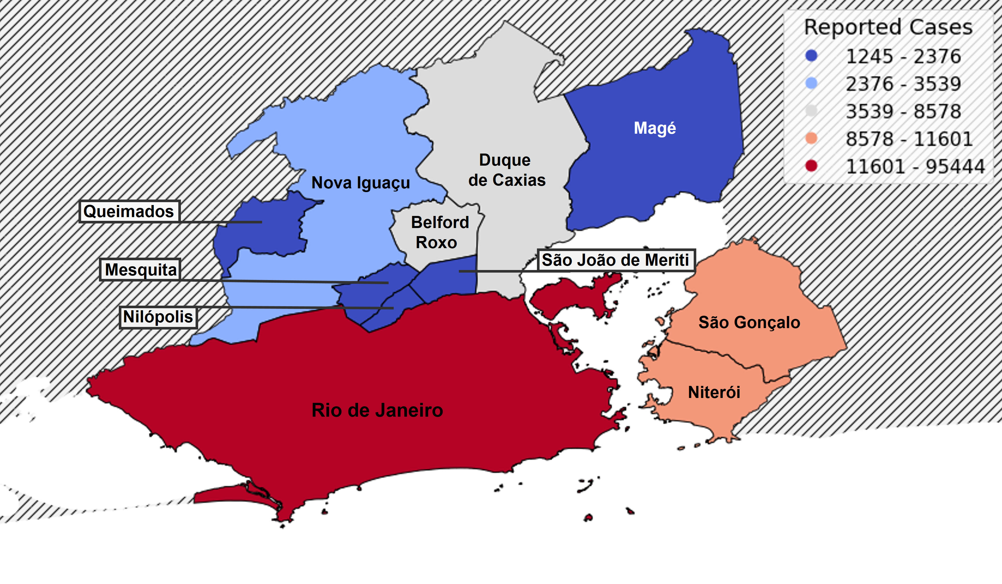
Supplementary Figure 1: Distribution of cases by the chosen cities of this study.

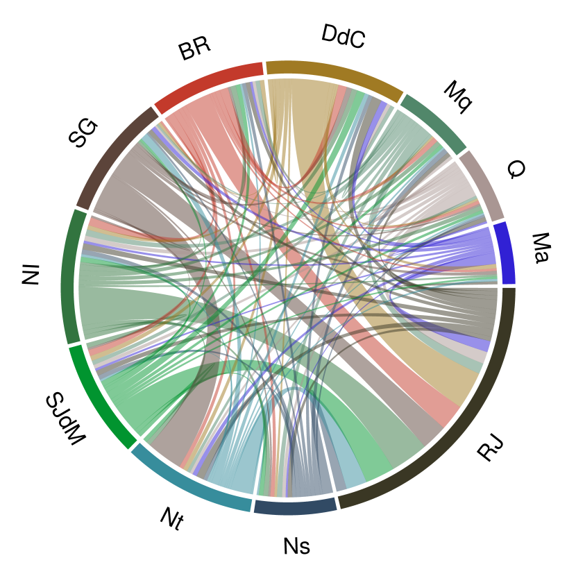
Supplementary Figure 2: Average daily commuter movement between municipalities, due to workplaces. The thickness of each line is proportional to the amount of movement from one municipality to another. Colors are used only for the purpose of better visualization and have no specific meaning.

- [1] Kermack, W. O. & McKendrick, A. G. A contribution to the mathematical theory of epidemics. Proceedings of the Royal Society of London (Series A) 115, 700–721 (1927).
- [2] Champredon, D., Dushoff, J. & Earn, D. J. Equivalence of the erlang-distributed seir epidemic model and the renewal equation. SIAM Journal on Applied Mathematics 78, 3258–3278 (2018).
- [3] Nishiura, H. & Chowell, G. The effective reproduction number as a prelude to statistical estimation of time-dependent epidemic trends. In Mathematical and statistical estimation approaches in epidemiology, 103–121 (Springer, 2009).
- [4] Oliveira, J. F. et al. Mathematical modeling of covid-19 in 14.8 million individuals in bahia, brazil .
- [5] Miranda, J. G. V. et al. Scaling effect in covid-19 spreading: The role of heterogeneity in a hybrid ode-network model with restrictions on the inter-cities flow. Physica D: Nonlinear Phenomena 415, 132792 (2021).
- [6] Jorge, D. C. et al. Assessing the nationwide impact of covid-19 mitigation policies on the transmission rate of sars-cov-2 in brazil. medRxiv (2020).
- [7] IBGE. Arranjos populacionais e concentrações urbanas no brasil (2016).