Dynamics of fluctuation correlation in a periodically driven classical system

Abstract

A many-body interacting system of classical kicked rotor serves as a prototypical model for studying Floquet heating dynamics. Having established the fact that this system exhibits a long-lived prethermal phase with quasi-conserved average Hamiltonian before entering into the chaotic heating regime, we use spatio-temporal fluctuation correlation of kinetic energy as a two-point observable to probe the above dynamic phases. We remarkably find the diffusive transport of fluctuation in the prethermal regime suggesting a novel underlying hydrodynamic picture in a generalized Gibbs ensemble with a definite temperature that depends on the driving parameter and the initial conditions. On the other hand, the heating regime is characterized by a diffusive growth of kinetic energy where the correlation is sharply localized around the fluctuation center for all time. Consequently, we attribute non-diffusive and non-localize structure of correlation to the crossover regime, connecting the prethermal phase to the heating phase, where the kinetic energy displays a complicated growth structure. We understand these numerical findings using the notion of relative phase matching where prethermal phase (heating regime) refers to an effectively coupled (isolated) nature of the rotors. We exploit the statistical uncorrelated nature of the angles of the rotors in the heating regime to find the analytical form of the correlator that mimics our numerical results in a convincing way.

Introduction.— In recent years periodically driven isolated systems emerge as an exciting field of research, giving justice to the fact that driven systems exhibit intriguing properties as compared to their equilibrium counterparts Shirley (1965); Dunlap and Kenkre (1986); Grifoni and Hänggi (1998). The quantum systems are studied extensively in this context theoretically Goldman and Dalibard (2014a); Eckardt (2017); Bukov et al. (2015a) as well as experimentally Wang et al. (2013); Rechtsman et al. (2013); Peng et al. (2016); Fleury et al. (2016); Maczewsky et al. (2017); for example, dynamical localization Kayanuma and Saito (2008); Nag et al. (2014, 2015), many-body localization D’Alessio and Polkovnikov (2013); D’Alessio and Rigol (2014); Ponte et al. (2015a, b); Lazarides et al. (2015); Zhang et al. (2016), quantum phase transitions Eckardt et al. (2005); Zenesini et al. (2009), Floquet topological insulator Oka and Aoki (2009); Kitagawa et al. (2011); Lindner et al. (2011); Rudner et al. (2013); Rodriguez-Vega et al. (2019); Seshadri et al. (2019); Nag et al. (2019a, 2020); Nag and Roy (2020), Floquet topological superconductor Ghosh et al. (2021a, b), Floquet time crystals Else et al. (2016); Khemani et al. (2016); Zhang et al. (2017); Yao et al. (2017), higher harmonic generation Faisal and Kamiński (1997); Nag et al. (2019b); Ikeda et al. (2018); Neufeld et al. (2019) are remarkable nonequilibrium phenomena. Consequently the heating happens to be very crucial factor as far as the stability of the driven systems is concerned Bilitewski and Cooper (2015); Reitter et al. (2017); Boulier et al. (2019). The consensus so far is that the driven quantum many-body systems heat up to an infinite-temperature state Moessner and Sondhi (2017); Luitz et al. (2017); D’Alessio and Rigol (2014); Seetharam et al. (2018) with some exceptions Prosen (1998); Haldar et al. (2018). However, it has been shown that heating can be suppressed for integrable systems due to infinite number of constants of motion, as manifested through the non-equilibrium steady states Russomanno et al. (2012); Nag et al. (2014); Gritsev and Polkovnikov (2017). On the other hand, many-body localized systems prevent heating for their effective local integrals of motion in the presence of interaction and disorder D’Alessio and Polkovnikov (2013); D’Alessio and Rigol (2014); Ponte et al. (2015a, b); Lazarides et al. (2015). The high frequency driving is another alternative route to prohibit the heating in the long-lived prethermal region, that grows exponentially with frequency, before heating up at the infinite temperature state  Choudhury and Mueller (2014); Bukov et al. (2015b); Citro et al. (2015); Mori (2015); Chandran and Sondhi (2016); Canovi et al. (2016); Mori et al. (2016); Lellouch et al. (2017); Weidinger and Knap (2017); Abanin et al. (2017a); Else et al. (2017); Zeng and Sheng (2017); Peronaci et al. (2018); Rajak et al. (2018); Mori (2018); Howell et al. (2019); Rajak et al. (2019); Abanin et al. (2017b).

Interestingly, the quasistationary prethermal state is concomitantly described by an effective static Hamiltonian, obtained using the Floquet-Magnus expansion, in the high-frequency regime Mori (2015); Canovi et al. (2016); Mori et al. (2016); Weidinger and Knap (2017); Abanin et al. (2017a); Else et al. (2017); Zeng and Sheng (2017); Peronaci et al. (2018). Here arises a very relevant question whether the classical systems exhibit such interesting intermediate prethermal plateau. Recently, using generic many-body systems of classical chaos theory Rajak et al. (2018, 2019) and periodically driven classical spin chains Howell et al. (2019); Mori (2018), the classical systems are also found to demonstrate the Floquet prethermalization. Similar to the quantum case, Floquet-Magnus expansion leads to an effective static classical Hamiltonian describing the prethermal phase where heating is exponentially suppressed Howell et al. (2019); Mori (2018); Rajak et al. (2019); Torre (2020); Hodson and Jarzynski (2021). The prethermal phase is further characterised by generalized Gibbs ensemble (GGE) causing hydrodynamic behavior to emerge in the above phase Castro-Alvaredo et al. (2016); Mori et al. (2018); Deutsch (2018).

The framework of fluctuating hydrodynamics becomes a convenient tool to investigate the equilibrium transport in classical non-linear systems Das and Dhar (2014); Mendl and Spohn (2013, 2014); Spohn (2014a); Mendl and Spohn (2015); Kundu and Dhar (2016); Dhar et al. (2019); Doyon (2019); Das et al. (2020). The integrable (non-integrable) classical systems typically admit ballistic (non-ballistic) transport Spohn (2014a); Das et al. (2014); Bastianello et al. (2018); De Nardis et al. (2018); Spohn (2020). The theory of fluctuating hydrodynamics is also employed to understand the transport in non-linear Fermi-Pasta-Ulam-Tsingou like systems Mendl and Spohn (2013); Das et al. (2014). Given the above background, we would like to investigate the non-equilibrium dynamics of fluctuation correlation of the kinetic energy in a model of interacting classical kicked rotors as a probe to the hydrodynamic behavior of the problem. The motivation behind choosing such model is that in the limit of large number of particles per site, a Bose-Hubbard model can be mapped to the above model Rajak et al. (2019). More importantly, kicked rotor systems can be realized in experiments using Josephson junctions with Bose-Einstein condensates Cataliotti et al. (2001). The time-periodic delta function kicks can be implemented by varying the potential depth and width controlling the intensity of laser light Cheneau et al. (2012); Goldman and Dalibard (2014b). The main questions that we pose in this work are as follows: How does a typical fluctuation behave in quasi-stationary prethermal states, as well as in the regime where kinetic energy grows in an unbounded manner Rajak et al. (2019)? Provided the notion of the GGE in the dynamic prethermal regime, does diffusive transport as seen for the case of static Hamiltonian Das et al. (2020) persist? Moreover, our questions are very pertinent experimentally where Floquet prethermalization has been realized in optical lattice platforms Messer et al. (2018); Rubio-Abadal et al. (2020).

Given the fact that the time-dynamics of the kinetic energy for the above system can be divided into three different temporal regimes depending on the nature of its growth Rajak et al. (2018, 2019), in this work, while numerically investigating the propagation of fluctuation (3) through the system as a function of time, we show that these dynamical regimes are characterized by distinct space-time behavior of the kinetic energy fluctuation correlation (see Fig. 1). Following the initial transient, the system enters into the prethermal regime, characterized by almost constant kinetic energy with exponentially suppressed heating, where the fluctuation spreads over space diffusively as a function of time (see Fig. 2). The spatio-temporal correlation becomes Gaussian whose variance $W$ increases linearly with time. Once the system starts absorbing energy from the drive, the fluctuation becomes exponentially localized around the site of disturbance and temporally frozen referring to the constant nature of $W$ with time (see Fig. 3). We refer this intermediate window as a crossover region that connects the spatially and temporally quasi-localized behavior of correlations at long time (see Fig. 4) with the prethermal phase. In that quasi-localized phase, $W$ decays to vanishingly small values while the kinetic energy of the system grows linearly with time. Therefore, the kinetic energy localization (diffusion) corresponds to the diffusion (localization) of fluctuation correlation. We qualitatively understand the underlying energy absorption mechanism in prethermal phase based on the hydrodynamic description. Our study considering fluctuation correlation of kinetic energy as a two-point observable, reveals new insight to the dynamic phases that are not accounted by the one-point observables. Moreover, dynamic features such as quasi-localization and localization of spatio-temporal correlations do not have any static analogue.

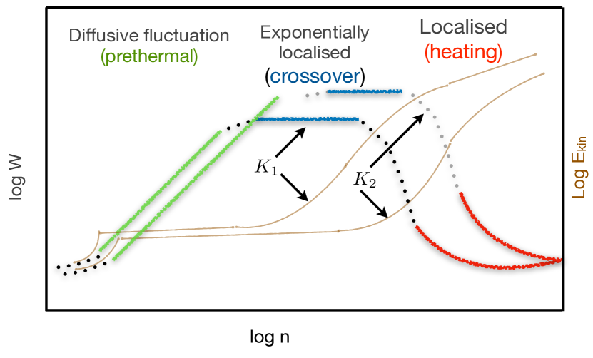
Figure 1: Schematic shows the evolution of relative width of spatio-temporal correlations (3), indicated by the log of variance $W$ (left axis), and the log of average kinetic energy per rotor $E_{\rm kin}(n)=(1/N)\sum^{N}_{j=1}\langle p^{2}_{j}(n)/2\rangle$ (right axis, brown solid line), as a function of number of kicks $n$ for two different values of driving parameters $K_{1}$ and $K_{2}$. The kinetic energy is quasi-conserved ($E_{\rm kin}(n)\sim n^{0}$, brown solid line) and the spread of spatio-temporal correlations is self-similar diffusive ($W\sim n$, green solid line) in the prethermal phase (see Fig. 2). The intermediate crossover regime is associated with non-diffusive growth of kinetic energy ($E_{\rm kin}(n)\not\sim n$, brown solid line) and temporally frozen correlations but exponentially localized in space ($W\sim n^{0}$, blue solid line), see Fig. 3. The diffusive growth of kinetic energy ($E_{\rm kin}(n)\sim n^{1}$, brown solid line) corresponds to heating regime where fluctuations tend to be almost $\delta$-correlated in space and time ($W\to 0$, with $n\to\infty$, red solid line), see Fig. 4. Interestingly, the lifetime of prethermal (heating) regime decrease (increases) with increasing driving parameter $K_{1}>K_{2}$. The different regimes of $W$ are connected by black (grey) dotted line for $K_{1}$ ($K_{2}$). We note that this plot is a cartoon representation while the exact numerical analysis for the evolution of the kinetic energy is given in Fig. $2$ of Ref. Rajak et al. (2019).

Model and correlation fluctuation.— We consider a generic non-equilibrium many-body system of classical chaos theory as given by Kaneko and Konishi (1989); Konishi and Kaneko (1990); Falcioni et al. (1991); Chirikov and Vecheslavov (1993, 1997); Mulansky et al. (2011); Rajak and Dana (2020).

$$H =\sum_{j=1}^{N}\left[\frac{p_{j}^{2}}{2}-\kappa\sum_{n=-\infty}^{+\infty}\delta(t-n\tau)V\left(r_{j}\right)\right],$$ (1)

where stretched variable $r_{j}=\phi_{j}-\phi_{j+1}$ and $V(r_{j})=1+\cos(r_{j})$. Here $\phi_{j}$, $j=1,\cdots,N$, are the angles of the rotors and $p_{j}$ are the corresponding angular momenta. The parameter $\kappa$ denotes the interaction as well as kick strength, and $\tau$ is the time period of delta kicks. The system described in Eq. (1) can have infinite energy density due to the unbounded nature of kinetic energy. We note that the total angular momentum of the system is an exact constant of motion, because the Hamiltonian in Eq. (1) is invariant under a global translation $\phi_{j}\rightarrow\phi_{j}+\alpha$, $\alpha$ being an arbitrary real number. Moreover, the Hamiltonian has discrete time translation symmetry $H(t)=H(t+\tau)$. Using classical Hamilton’s equations of motion, one can get the discrete maps of $\phi_{j}$ and $p_{j}$ between $n$-th and $(n+1)$-th kicks:

$$p_{j}(n+1) =p_{j}(n)-\kappa\left(V^{\prime}(r_{j-1})-V^{\prime}(r_{j})\right)$$

$$\phi_{j}(n+1) =\phi_{j}(n)+p_{j}(n+1)\tau.$$ (2)

Here $V^{\prime}$ describes derivative of $V$ with respect to $r_{j}$ evaluated after $n$-th kick. We consider periodic boundary conditions $\phi_{N+i}=\phi_{i}$. From Eq. (2), it can be noticed that the dynamics of the system is determined by only one dimenisonless parameter, $K=\kappa\tau$ that we use for all our further calculations  Rajak et al. (2018, 2019).

We compute here the spatio-temporal correlation of kinetic energy fluctuations, defined by

$$C(i,j,t,t_{w})=\frac{1}{4}\left[\langle{p_{i}^{2}(t)}{p_{j}^{2}(t_{w})}\rangle-\langle{p_{i}^{2}(t)}\rangle\langle{p_{j}^{2}(t_{w})}\rangle\right],$$ (3)

where $i$ and $j$, respectively, represent the positions of $i$-th and $j$-th rotors; $t$ ($t_{w}$) represents an arbitrary final time (initial waiting time). We always consider $t>t_{w}$ throughout the paper. The symbol $\langle..\rangle$ denotes the average over the initial conditions where $\phi_{j}(0)$ are chosen from a uniform distribution $\in[-\pi,\pi]$, and the corresponding momenta, $p_{j}(0)=0$ for $j=1,\cdots,N$. The spatio-temporal correlation captures how a typical small perturbation applied at time $t_{w}$ spreads in space $x\equiv i-j$ (with translation symmetry) and time $t$ through the system. We refer to the correlator in Eq. (3) as $C(x,t)$ while investigating below. The system shows an exponentially long prethermal state where the kinetic energy becomes almost constant, and eventually heats up after a crossover regime when the kinetic energy grows linearly with time Rajak et al. (2018, 2019). We have further analyzed different temporal regimes investigating the behavior of spatio-temporal correlation. The prethermal state can be characterized appropriately by a time-averaged Hamiltonian (see Eq. (5)). Therefore, although, the driven system breaks continuous time-translation symmetry, it preserves an effective time-translation symmetry inside the prethermal regime due to quasi-conservation of Floquet Hamiltonian at high frequencies. Thus, the spatio-temporal correlator becomes a function of space $x\equiv i-j$ and time $t\equiv t-t_{w}$ inside the prethermal regime. However, for other two regimes where the total energy is not a constant of motion, the correlator generally becomes a function of both $t$ and $t_{w}$ in addition to $x$.

We have summarized our main result of spatio-temporal correlation and its connection with the evolution of kinetic energy schematically in Fig. 1. In this context, we consider the width of the spatio-temporal correlations, i.e., variance

$$W=\frac{\sum_{x=-N/2}^{N/2}x^{2}C(x,t)}{\sum_{x=-N/2}^{N/2}C(x,t)},$$ (4)

to characterize different dynamical regimes. In order to measure the relative width of the fluctuations, the appropriate normalization of the distribution as described by the denominator is crucial. In the prethermal regime, the denominator is independent of time due to conservation of energy, while in the other regimes, the denominator is time dependent and normalizes the distribution at all times. We have schematically drawn the evolution of $W$ in Fig. 1 by acquiring detailed knowledge about spatio-temporal correlation in different phases as discussed below.

The observables are averaged over $10^{5}$ to $10^{6}$ initial conditions. Otherwise specifically mentioned in our simulations, we fix $\tau=1$ and $N=2048$. This makes $t=n$, and we use these terms interchangeably. The lifetime of the prethermal state for such systems (see Eq. (1)) increases exponentially in $1/K$ Rajak et al. (2019). For small values of $K$, the prethermal state persists for astronomically large time, thus making the numerical calculation extremely costly to probe all the dynamical phases by varying time. In order to circumvent this problem, we choose to tune $K$ such that the lifetime of the prethermal state can be substantially minimized and we can investigate the phase where fluctuations get localized within our numerical facilities. However, provided the distinct nature of these regimes, our findings would remain unaltered if one addresses them by varying time only. In our numerical calculations, we choose both $t,~{}t_{w}$ within the same phase.

We would like to emphasize the choice of $t$ and $t_{w}$ such that the fluctuation correlation of kinetic energy can behave distinctly in different regimes. There can be some quantitive but no qualitative changes in the correlator for $t$ and $t_{w}$ chosen from same regimes while quantitive changes are observed for $t$ and $t_{w}$ chosen from different regimes. In order to give an idea about the choice of $t$ and $t_{w}$, we exemplify a situation with $K=0.3$ where $10^{1}<t,~{}t_{w}<10^{3}$ for prethermal regime, $6\times 10^{3}<t,~{}t_{w}<10^{4}$ for the crossover regime and $2\times 10^{5}<t,~{}t_{w}<10^{7}$ for the heating regime Rajak et al. (2019). As discussed above the temporal width of various regimes vary with $K$ and hence $t$ and $t_{w}$ are needed to be appropriately chosen within the same regimes.

Results.— We first focus on the spreading of fluctuation (3) in the prethermal phase that is denoted by the green solid lines in Fig. 1. The prethermal phase can be described by a GGE with the total energy as a quasi-conserved quantity Rajak et al. (2019). In terms of the inverse frequency Floquet-Magnus expansion, the lowest order term of the Floquet Hamiltonian is the average Hamiltonian that governs the prethermal state at high frequency, given by

$$H^{*}=\frac{1}{\tau}\int_{0}^{\tau}H(t)dt=\sum_{j=1}^{N}\left[\frac{p_{j}^{2}}{2}-\frac{\kappa}{\tau}\left(1+\cos\left(\phi_{j}-\phi_{j+1}\right)\right)\right].$$ (5)

Employing the notion of GGE, the composite probability distributions can be written as

$$P^{*}(\{p_{j},r_{j}\})=\frac{1}{Z^{*}}\prod_{j=1}^{N}e^{-\big{(}\frac{p_{j}^{2}}{2}-\frac{\kappa V(r_{j})}{\tau}\big{)}/T^{*}},$$ (6)

where $Z^{*}$ is the partition function for the GGE and $T^{*}$ is the temperature associated with prethermal phase. Given the particular choice of the initial conditions here, the prethermal temperature is found to be $T^{*}=0.938363\frac{K}{\tau^{2}}$ Rajak et al. (2019); for more details see Appendix A. Moreover, this description of the GGE does not depend on the number of rotors $N$, thus indicating the thermodynamic stability of this phase.

We associate the prethermal phase with the diffusive spatio-temporal spread of kinetic energy correlation as shown in Fig. 2 (a). A relevant renormalization of $x$ and $y$-axes with time yields the following scaling form of the correlation: $C(x,t)\sim A_{K}t^{-1/2}f\big{(}xt^{-1/2}\big{)}$, with $f(y)=e^{-y^{2}/2D}/\sqrt{2\pi D}$, as depicted in Fig. 2 (b); for more detailed discussions see Appendix B. We thus find that the correlation at different space time collapse together. Here, $A_{K}$ denotes the amplitude of the Gaussian distribution respectively for a given value of $K$. The diffusion constant $D$ is a measure of variance $W$, being weakly dependent on the parameter $K$, grows linearly with time $W\sim t$. One can observe that the fluctuation spreads in a way such that the area under the correlation curves keep their area constant i.e. the sum rule $\sum_{x}C(x,t)$ is approximately independent of time in the prethermal phase. The sum rule determines $A_{K}=\sum_{x=-N/2}^{N/2}C(x,t)\approx\sum_{x=-N/2}^{N/2}C(x,0)=\delta_{x,0}\left(\langle p^{4}\rangle-\langle p^{2}\rangle^{2}\right)/4=0.4402K^{2}/\tau^{4}\delta_{x,0}$, by considering the fact that the energy absorption is exponentially suppressed in the prethermal regime Rajak et al. (2019); for more details see Appendix A. This supports our numerical result of quadratic growth of $A_{K}$ as shown in the inset of Fig. 2 (b). The apparent $27\%$ mismatch in the prefactor of $A_{K}$ with the numerically value might be due to the fact that exponentially slow variation of the kinetic energy in the prethermal phase is not taken into account theoretically.

The energy correlations of static rotor system at high temperature platform exhibit diffusive transport Lepri (2016); Dhar (2008). This is in resemblance with the present case of Floquet prethermalization at high frequency. Owing to the quasi-validity of equipartition theorem in the GGE picture Rajak et al. (2018, 2019), the kinetic and potential energy behave in an identical fashion. As a result, the correlation of total energy qualitatively follows the correlation of kinetic energy in the prethermal regime.

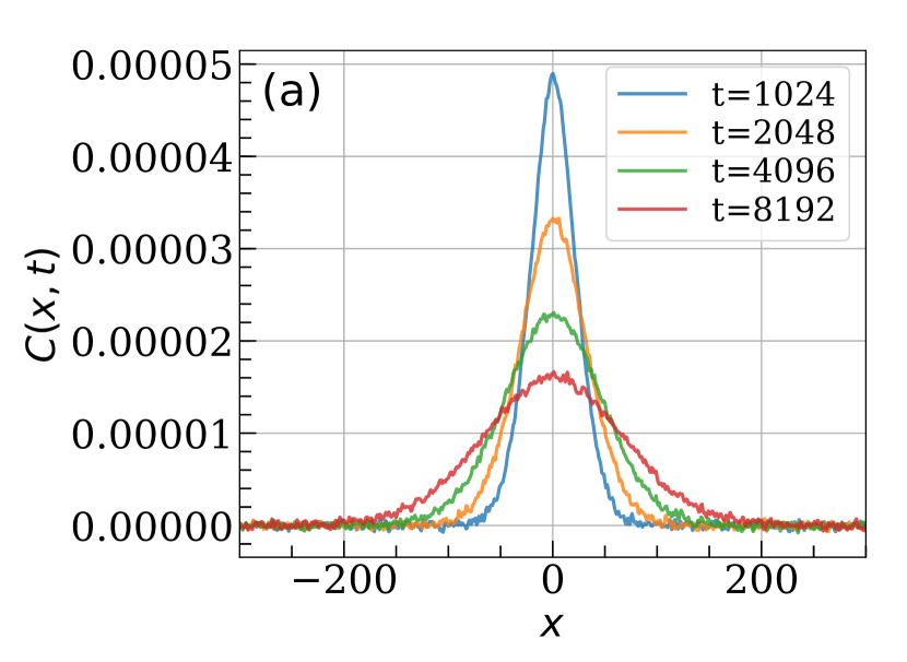
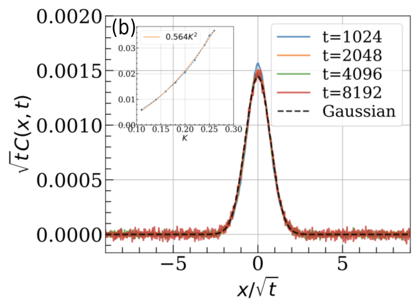
Figure 2: (a) The space-time spreading of kinetic energy correlation (3) for $K=0.14$ in the prethermal regime. (b) The diffusive Gaussian scaling of correlation is observed with appropriate renormalization: $C(x,t)=A_{K}t^{-1/2}f(xt^{-1/2}),~{}f(y)=e^{-y^{2}/2D}/\sqrt{2\pi D}$ with parameters $D\sim 0.727$ and $A_{K}\sim 0.0026$. Inset shows the quadratic variation of the total area under the curve $\sum_{x=1}^{N}C(x,t)$ with $K$. The parameters are $N=2048$, and $t_{w}=64$.

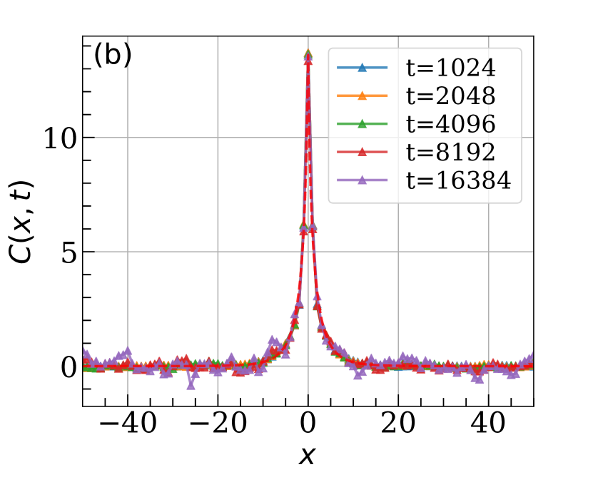
Figure 3: The space-time spreading of kinetic energy correlation (3) for (a) $K=0.45$, $t_{w}=142$ and $K=0.7$, $t_{w}=64$ (b), respectively, in the intermediate crossover regime. The correlation distribution is fitted with stretched exponential $C(x,t)\sim\frac{A_{K}}{2\alpha^{-1/\beta}\Gamma\left(1+\frac{1}{\beta}\right)}e^{-\alpha|x|^{\beta}}$ with $\alpha\sim 0.36~{}[1.05],\beta\sim 0.63~{}[0.65],A_{K}\sim 5.16~{}[41.51]$ for (a) [(b)]. The system size is $N=2048$ for both cases.

We now investigate the spatio-temporal evolution of correlation (3) in the intermediate crossover regime, designated by the blue solid line in Fig. 1, that lies between the prethermal and the heating region of kinetic energy. The system starts to absorb energy from the drive through many-body resonance channels causing the kinetic energy to grow in sub-diffusive followed by super-diffusive manner Rajak et al. (2018, 2019). However, the probability of the occurrence of such resonances decreases exponentially with $1/K$ in the high frequency limit. We find that the oscillators are maximally correlated with each other at $x=0$ and falls rapidly to zero in two sides $x$ as shown in Fig. 3 (a) and (b), for $K=0.45$ and $0.7$, respectively. To be precise, correlation decays stretched exponentially in short distances: $C(x,t)\sim A_{K}e^{-\alpha|x|^{\beta}}$ while it falls exponentially (i.e., more rapidly than stretched exponential) in long distances: $C(x,t)\sim e^{-\gamma|x|}$; for more details see Appendix D. Here, $\beta$ and $\gamma$ weakly depend on $K$ referring to the fact that driving parameter $K$ can in general control the spatial spread of fluctuation. These profiles do not change with time within the crossover region referring to the fact that variance of the spatial correlation distribution remains constant with time $W\sim t^{0}$. This allows us to differentiate it from the diffusive transport that occurs in the prethermal phase. However, with increasing time, one can observe that long distance correlation becomes more noisy leaving the spatial structures qualitatively unaltered.

At the end, we discuss the time zone where the average kinetic energy shows unbounded chaotic diffusion, as denoted by the red solid line in Fig. 1, resulting in the effective temperature to increase linearly with time Rajak et al. (2018, 2019). The correlation of the kinetic energy is fully localized in space and temporally frozen as shown in Fig. 4). To be precise, the correlation is nearly a $\delta$-function centered around $x=0$ i.e., fluctuation gets localized at the site of disturbance for all time. In this regime, the system shows fully chaotic behavior in the phase space and the angles of the rotors become statistically uncorrelated both in space and time. It is noteworthy that there is no description of average Hamilton exist here as the inverse frequency Floquet-Magnus expansion does not converge Mori (2018); Howell et al. (2019). In contrast to the prethermal phase, the amplitude of correlation peak in the crossover and heating regime increases as $K^{\eta}$ with $\eta>2$. On the other hand, the variance in the heating regime becomes decreasing function of $n$, precisely, $W\to 0$ for $n\to\infty$ that is markedly different from the behavior of $W$ in remaining two earlier regimes. Finally, we stress that our findings in this heating regime do not suffer from finite size effect suggesting the thermodynamic stability of this phase.

It is noteworthy that $\langle{p_{i}^{2}(t)}{p_{j}^{2}(t_{w})}\rangle$ and $\langle{p_{i}^{2}(t)}\rangle\langle{p_{j}^{2}(t_{w})}\rangle$ in the kinetic energy fluctuation both individually depend on time $t$ and the initial waiting time $t_{w}$. On the contrary, the connected part i.e., $C(i,j,t,t_{w})$ as a whole does not depend on $t$ instead depends on $t_{w}$ such that the peak height of $C(i,j,t,t_{w})$-profile increases with $t_{w}$. This can be physically understood as an initial value problem in terms of $p_{i,j}(t_{w})$ for the rotors that subsequently uncorrelated in the heating region. The peak value of the correlator is also found to be dependent on the coupling parameter $K$. In this region, the time-independent correlator effectively freezes into three discrete spatial points i.e., at the site of disturbance with $i=j$ and the remaining two adjacent sites with $i=j\pm 1$.

We shall now exploit the assumption of statistically uncorrelated (both in space and time) nature of the rotors to shed light on this intriguing behavior analytically. In terms of the stretched variable $r_{j}(n)=\phi_{j+1}(n)-\phi_{j}(n)$, the assumption leads to the following mathematical form

$$\langle\sin(r_{i}(n))\sin(r_{j}(m))\rangle=\frac{1}{2}~{}\delta_{n,m}\delta_{i,j},$$

$$\langle\sin(r_{i}(n))\sin(r_{j}(n^{\prime})\sin(r_{k}(m))\sin(r_{l}(m^{\prime}))\rangle=$$

$$\frac{1}{4}~{}(\delta_{n,n^{\prime}}\delta_{m,m^{\prime}}\delta_{i,j}\delta_{k,l}+\delta_{n,m}\delta_{n^{\prime},m^{\prime}}\delta_{i,k}\delta_{j,l}$$

$$+\delta_{n,m^{\prime}}\delta_{n^{\prime},m}\delta_{i,l}\delta_{j,k})+\frac{3}{8}\delta_{n,n^{\prime}}\delta_{m,m^{\prime}}\delta_{m,n}\delta_{i,j}\delta_{k,l}\delta_{i,k}$$ (7)

where the average is carried over different initial conditions, $i,j,k,l$ represent the position of the rotor and $n,n^{\prime},m,m^{\prime}$ denote the various times $t$’s in terms of the number of kicks. We note that $r_{j}(n)$ becomes uniform random variable in the heating region. The momentum of $i$-th rotor at any time $t$ can be formulated from the equation of motion (Eq. 2). The first term of the kinetic energy fluctuation correlator with $t>t_{w}\gg 1$ can be calculated in the heating regime as follows

$$\langle p_{i}^{2}(t)p_{j}^{2}(t_{w})\rangle=K^{4}\Big{(}2~{}t_{w}^{2}\delta_{i,j}+\frac{1}{2}~{}t_{w}^{2}\delta_{i,j+1}+\frac{1}{2}t_{w}^{2}\delta_{i,j-1}$$

$$+\frac{3}{4}t_{w}\delta_{i,j}+\frac{3}{8}~{}t_{w}\delta_{i,j+1}+\frac{3}{8}~{}t_{w}\delta_{i,j-1}+tt_{w}\delta_{i,i}\delta_{j,j}\Big{)}.$$ (8)

The last term reminds us the diffusive growth of kinetic energy $\langle p_{i}^{2}(t)\rangle=K^{2}t$ that is obtained in the heating region. Therefore, the kinetic energy fluctuation correlation (Eq. (3)) takes the following form

$$C(i,j,t,t_{w})=K^{4}\Big{(}\frac{t_{w}^{2}}{2}\delta_{i,j}+\frac{3t_{w}}{16}\delta_{i,j}+\frac{t_{w}^{2}}{8}\delta_{i,j+1}+\frac{3t_{w}}{32}\delta_{i,j+1}$$

$$+\frac{t_{w}^{2}}{8}\delta_{i,j-1}+\frac{3t_{w}}{32}\delta_{i,j-1}\Big{)}$$

$$=K^{4}\Big{(}\frac{t_{w}^{2}}{2}\delta_{i,j}+\frac{t_{w}^{2}}{8}\delta_{i,j+1}+\frac{t_{w}^{2}}{8}\delta_{i,j-1}\Big{)}+O(t_{w})$$ (9)

We note that for $t_{w}\gg 1$, the $O(t^{2}_{w})$ terms dominate over $O(t_{w})$ term. This clearly suggests that the assumption of uncorrelated nature of rotors is able to mimic the numerical outcome convincingly in the heating region i.e., $C(x,t)\neq 0$ for $x=0$ and $\pm 1$. In Fig. 4, we compare the numerical results with the prediction of Eq. 9 and find a match within $6\%$ error. The above result is derived considering the assumption that rotors are always uncorrelated under driving. As a result, the independent rotor approximation works better to explain the numerical outcomes for higher values of $K$ as the driven system enters into the heating region quite early. Most importantly, the analytical form in Eq. (9) correctly captures the value of the correlator at the adjacent sites of the disturbance $i=j\pm 1$ drops to $\frac{1}{4}$ of the peak value at $i=j$, as observed in Fig. 4. The non-zero value of correlation in the adjacent sites might be the effect of nearest-neighbor interactions of the system. In addition, the correlator is independent of final time $t$, whereas it depends on $t_{w}$, when the disturbance is applied on the system. It indicates that the correlator depends on the value of momentum at $t=t_{w}$, from where we start measuring the correlator, but correlator does not spread further with time since the rotors are effectively uncorrelated in this regime. The detailed analytical derivation is presented in Appendix E.

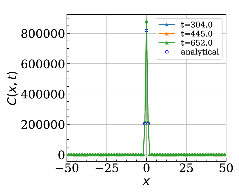
Figure 4: The correlations (3) become fully localized such as nearly a $\delta$-function in the heating region for $K=3$, with $t_{w}=142$, $N=2048$. The blue circles denote the correlation values as a function of initial wait time and the kick strength given by Eq. 9.

We here stress that Fig. 1, being a cartoon representation, can compactly demonstrate the results shown in Figs. 2, 3, and 4 as well as shed light on the physical understanding. We superimpose the time evolution of the variance $W$ of the correlation $C(x,t)$, obtained from analyzing the correlation profile in Figs. 2, 3, and 4, with the kinetic energy $E_{\rm kin}(n)$ that has already been reported Rajak et al. (2019). In the prethermal regime, $E_{\rm kin}(n)\sim n^{0}$ and the self-similar Gaussian scaling of $C(x,t)\sim f(xt^{-1/2})$ suggests $W\sim n$ (see Fig. 2(b)). In the crossover region, $E_{\rm kin}\not\sim n$ and the temporally frozen stretched exponential $C(x,t)\sim f(x,t^{0})$ yields $W\sim n^{0}$ (see Fig. 3). In the heating region, $E_{\rm kin}\sim n$, fluctuations become nearly $\delta$-correlated but frozen in time $C(x,t)\sim f(x,t^{0})\delta_{x,l}$ with $l\in[0,\pm 1]$, leads to the following situation $W\to 0$ as $n\to\infty$ (see Fig. 4). Therefore, the disjoint nature between the spatial and temporal structures of the correlation in crossover and heating regions causes distinct features in $W$ as compared to its combined spatio-temporal nature for prethermal region.

Discussions.— This is clearly noted in our study that the spatio-temporal correlation provides a deep insight to characterize different dynamical phases. The phase matching between adjacent rotors, captured by stretched variables $r_{j}(n)=\phi_{j+1}(n)-\phi_{j}(n)$, play very important role in determining the nature of spreading of the fluctuations. The time-evolution of the stretched variable, following the equations of motion (2), is given as $r_{j}(n+1)=r_{j}(n)+(p_{j+1}(n+1)-p_{j}(n+1))\tau$. Upon satisfying the resonance condition $p_{j}-p_{j+1}=2\pi m/\tau$ with $m$ as an integer number, the stretched variable rotates by $2\pi$ angle between two subsequent kicks. When all the rotors go through these resonances, their relative phase matching is lost and the eventually the coupled rotor system turned into an array of uncoupled independent rotor. At this stage, the system absorbs energy from the drive at a constant rate in an indefinite manner. This is precisely the case for heating up regime where fluctuation correlations do not spread in time and space. On the other hand, the resonances are considered to be extremely rare events in the prethermal regime suggesting the fact that relative phase matching between adjacent rotors allows the fluctuation to propagate diffusively throughout the system in time. The notion of the time independent average Hamilton in the prethermal region might be related to the fact that all the rotors rotate with a common collective phase and eventually controlled by an underlying synchronization phenomena Nag et al. (2019b); Khasseh et al. (2019).

Coming to the phenomenological mathematical description, the exponential suppressed heating and the validity of the constant sum-rule in the prethermal phase suggest a hydrodynamic diffusion picture (with diffusion constant $D$) for the fluctuation Spohn (2014b, 2016); Dhar et al. (2021); Ye et al. (2020):

$$\partial_{t}u(x,t)=\partial_{x}\bigg{(}\frac{D}{2}~{}\partial_{x}u(x,t)+B~{}\zeta(x,t)\bigg{)}$$ (10)

where $u(x,t)=\frac{1}{2}\left(p^{2}(x,t)-\langle p^{2}(x,t)\rangle\right)$ such that $\langle p^{2}(x,t)\rangle\neq\langle p^{2}(x,t^{\prime})\rangle$. The conservative noise $\zeta(x,t)$ of strength $B$ is delta correlated in space and time $\langle\zeta(x,t)\zeta(x^{\prime},t^{\prime})\rangle=\delta_{xx^{\prime}}\delta(t-t^{\prime})$. In the high-frequency limit, the equilibrium fluctuation dissipation relation can be extended to long-lived prethermal regime: $B^{2}\sim D{T^{*}}^{2}$; for more details see Appendix C. Given the plausible assumption that the noise part $B$ of the fluctuating current increases with increasing $K$, one can understand the diffusion process in a phenomenological way. The diffusion constant $D$ is then considered to be independent of $K$ while prethermal temperature is determined by $K$, as observed in GGE picture. Moreover, the self-similar Gaussian nature of fluctuation correlation in the prethermal phase can be understood from the solution of Eq. 10 such that $C(x,t)\sim\langle u^{2}(0,\tau_{i})\rangle e^{-x^{2}/(2Dt)}/\sqrt{2\pi Dt}$. In the other limit inside the infinite temperature heating regime, the non-diffusive transport leaves the $u(x,t)$ to be $\delta$ correlated in space while almost frozen in time. Now there is an extended crossover region, connecting the prethermal state to heating regime, where the diffusion equation does not take such simple form causing the system to exhibit an amalgamated behavior.

Before we conclude, we would like to re-emphasize that unlike the equilibrium case $t_{w}$ plays crucial role for the non-equilibrium case. To be more precise, only relevant time variable is the relative time $t\equiv t-t_{w}$ for equilibrium case respecting time translation symmetry. This is not true in the present case and the correlation is expected to exhibit complex structure for arbitrarily chosen $t$ and $t_{w}$ with $t>t_{w}$. Thanks to the GGE description of the prethermal region, we can consider the relative time $t\equiv t-t_{w}$ as the appropriate variable. One can think of the average Hamiltonian embeds an effective time translation symmetry in the prethermal phase. However, the effective GGE description fails for crossover and heating region, resulting in the fact that the two time instants $t$ and $t_{w}$ are equally important there. The effective time translation symmetry is no longer valid in the above two regions. This is what we clearly see for the heating regime where the peak value of the correlator depends on $t_{w}$.

Conclusions.— In conclusion, our study demonstrates that a typical two-point observable such as, the fluctuation correlation of kinetic energy, can be scrutinized to probe different dynamic phases of classical many-body kicked rotor system com . It is indeed counter intuitive that the average kinetic energy per rotor and their spatio-temporal correlations, being derived from the former quantity, yet yield opposite behavior. The GGE description of prethermal phase obeys diffusive transport where spatio-temporal correlation follows self similar Gaussian profile. During this diffusion, the correlation curves keep their area constant due to the quasi-conservation of the kinetic energy. In the long time limit where kinetic energy grows diffusively, fluctuation interestingly becomes frozen in space and time. We have also calculated the behavior of kinetic energy fluctuation analytically using the statistically uncorrelated nature of the angles of the rotors inside the heating regime and find a good match with the numerical results. There exists an extended crossover region where kinetic energy increases in a complicated way exhibiting both sub-diffusive to super-diffusive nature. The fluctuation interestingly shows a rapidly (slowly) decaying short (long) range stretched (regular) exponential localization. In this case the fluctuation does not have any time dynamics. Therefore, correlated phenomena in prethermal phase gradually assembles to completely uncorrelated heat up phase through a crossover region. These non-trivial phases of matter are the consequences of the driving and do not have any static analogue. Provided the understanding on long range quantum systems Lerose et al. (2019); Saha et al. (2019); De Tomasi (2019); Nag and Garg (2019); Modak and Nag (2020a, b), it would be interesting to study the fate of the above phases along with the crossover region in long-range classical systems. Furthermore, various intriguing nature of correlators can be observed for $t$ and $t_{w}$ chosen from different phases that is beyond the scope of the present study. The microscopic understanding of hydrodynamic picture and fluctuation-dissipation relation in dynamic systems are yet to be extensively analyzed in future.

Acknowledgement : We thank Andrea Gambassi and Emanule Dalla Torre for reading the manuscript and their constructive comments. A.R. acknowledges UGC, India for start-up research grant F. 30-509/2020(BSR). AK would like to thank the computational facilities Mario at ICTS and Ulysses at SISSA.

Appendix A Gibbs distribution in prethermal phase

Assuming that in the prethermal region, the ensemble is goverened by a Gibbs ensemble with

$$P^{*}=(Z^{*})^{-1}e^{-\left(H^{*}+\gamma\bar{p}+\delta\tilde{r}\right)/\left(T^{*}\right)},$$ (11)

where $\bar{p}=\sum_{j=1}^{N}p_{j}$ and $Z^{*}=\int dpdre^{-\left(H^{*}+\gamma\tilde{p}+\delta\tilde{r}\right)/T^{*}}$ are the total angular momentum and the GGE partition function of the system, respectively Rajak et al. (2019). Equating the initial energy with the GGE average energy, we obtain the effective temperature of the system. The kinetic energy $E_{\mathrm{kin}}$ of the driven system in the prethermal phase is given by

$$E_{\mathrm{kin}}=\frac{1}{N}\sum_{j=1}^{N}\int\frac{p_{j}^{2}}{2Z^{*}}\prod_{j^{\prime}=1}^{N}e^{-\left(p_{j^{\prime}}-\tilde{p}\right)^{2}/\left(2T^{*}\right)}dp_{j^{\prime}}=\frac{T^{*}+\tilde{p}^{2}}{2},$$ (12)

where $\tilde{p}=\gamma T^{*}/N$ with $\gamma$ being a constant. On the other hand, the total energy in this phase is given by

$$E^{*}=\sum_{j=1}^{N}\frac{\left\langle p_{j}^{2}\right\rangle_{*}}{2}+\frac{\kappa}{\tau}\sum_{j=1}^{N}\left\langle 1-\cos\left(\phi_{j}-\phi_{j+1}\right)\right\rangle_{*}.$$ (13)

The potential energy and total energy take the following from

$$\langle 1-\cos(r_{j})\rangle_{*} = (Z^{*})^{-1}\int dr(1-\cos(r_{j}))e^{-\frac{\kappa}{\tau T^{*}}(1-\cos(r_{j}))}$$

$$= 1-\frac{I_{1}(\epsilon)}{I_{0}(\epsilon)}$$

$$E^{*} = N\frac{T^{*}+\tilde{p}^{2}}{2}+\frac{N\kappa}{\tau}\left(1-\frac{I_{1}(\epsilon)}{I_{0}(\epsilon)}\right)$$ (14)

with $\epsilon=\kappa/(T^{*}\tau)$ and $I_{n}(x)$ denotes the modified Bessel’s function of order $n$ for the argument $x$.

The micro-canonical initial energy of the system is $E_{0}=N\frac{\tilde{p}^{2}}{2}+N\frac{\kappa}{\tau}$. Now neglecting the initial growth of the kinetic energy in the transient phase and quasi-conserved nature of kinetic energy in prethermal phase, one can consider $E_{0}\simeq E^{*}$. One thus arrives at the following

$$\frac{1}{\epsilon}+\left(\frac{I_{1}(\epsilon)}{I_{0}(\epsilon)}\right)=0\implies\epsilon=1.06569.$$ (15)

This implies $T^{*}=0.938363\frac{\kappa}{\tau}$. In the prethermal phase (with $\tilde{p}=0$ ), the average energy is then given by

$$E^{*}/N = \frac{T^{*}}{2}+\frac{\kappa}{\tau}\left(1-\frac{I_{1}(\epsilon)}{I_{0}(\epsilon)}\right)=\frac{\kappa}{\tau}\Big{(}\frac{0.938363}{2}+0.530819\Big{)}$$ (16)

$$= \frac{\kappa}{\tau}.$$

One can redefine the standard energy per-site, which is equivalent to average energy pumped into the site over a time period. In the prethermal phase, the probability distribution of kinetic and potential energies take the form

$$P^{*}(p)=\prod_{j^{\prime}=1}^{N}e^{-\left(p_{j^{\prime}}\right)^{2}/\left(1.876\frac{\kappa}{\tau}\right)}$$ (17)

$$P^{*}(r_{j})=\prod_{j^{\prime}=1}^{N}e^{-\left(1-\cos(r_{j})\right)/1.876}$$ (18)

The specific heat at constant volume can be obtained at the prethermal value as $C_{v}=\partial E/\partial T|_{T^{*}}$ with

$$E = \frac{T^{*}}{2}+\frac{\kappa}{\tau}\left(1-\frac{I_{1}(\kappa/(T^{*}\tau)}{I_{0}(\kappa/(T^{*}\tau)}\right)$$ (19)

$$C_{v} = \partial E/\partial T|_{T^{*}}=\frac{\kappa^{2}}{\tau^{2}{T^{*}}^{2}}-\frac{\kappa^{2}I_{1}\left(\frac{\kappa}{{T^{*}}\tau}\right){}^{2}}{\tau^{2}{T^{*}}^{2}I_{0}\left(\frac{\kappa}{{T^{*}}\tau}\right){}^{2}}$$ (20)

$$- \frac{\kappa I_{1}\left(\frac{\kappa}{{T^{*}}\tau}\right)}{\tau{T^{*}}I_{0}\left(\frac{\kappa}{{T^{*}}\tau}\right)}+\frac{1}{2}$$

$$= 0.88572.$$

Note that this value is independent of the driving frequency in the prethermal regime. It implies that the system absorbs heat at a constant rate irrespective of the driving frequency in the prethermal state.

The correlation functions assuming the system is in the prethermal GGE can be computed from the sum rule such that area under the correlation curves keep their area constant, $A_{K}=\sum_{x}C(x,t)\approx\frac{1}{4}(\langle p^{4}\rangle-\langle p^{2}\rangle^{2})$, where the average is defined as, $\langle y(p)\rangle=\int_{-\infty}^{\infty}dp~{}y(p)~{}e^{-p^{2}/T^{*}}/\int_{-\infty}^{\infty}dp~{}e^{-p^{2}/T^{*}}$. We find $A_{K}\sim 2{T^{*}}^{2}/4=1.72348K^{2}/4=0.4402K^{2}/\tau^{4}.$ We analyze this sum rule $A_{K}$ in the Fig. 2 (b) of the main text.

Appendix B Exponentially suppressed variation of prethermal temperature and diffusion constant

In the prethermal regime, the average kinetic energy is slowly changing in time, and heating is exponentially suppressed. This is shown in Fig. 5 (a), where the ratio of the prethermal temperature at time $t$ and $t_{w}$, defined by $\sum_{i}p_{i}(t)^{2}/\sum_{i}p_{i}(\tau_{w})^{2}$, is analyzed. The almost constant nature of variable $T(t)/T(t_{w})$ signifies that the temperature is not significantly changing with time. For high frequency drive with $K=0.14$, the temporal extent of the prethermal region is larger than that of the for $K=0.24$. These clearly indicate that the departure from the prethermal phase is caused by low frequency drive with higher values of $K$. We present this result in Fig. 1 of the main text. On the other hand, the unsubtracted correlation functions $\langle{p_{i}^{2}(t)}{p_{j}^{2}(t_{w})}\rangle$ in the prethermal region with $K=0.14$ are shown in Fig. 5 (b) referring to the drifts for the correlation in time. We note that correlation propagates even into the substantially separated rotors from fluctuation core at $x=0$. However, once the connected part is subtracted, the correlations decay to zero away from the $x=0$, which suggest the hydrodynamic picture as discussed in the main text.

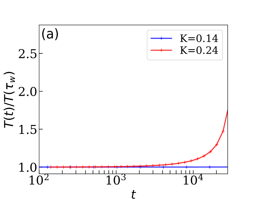
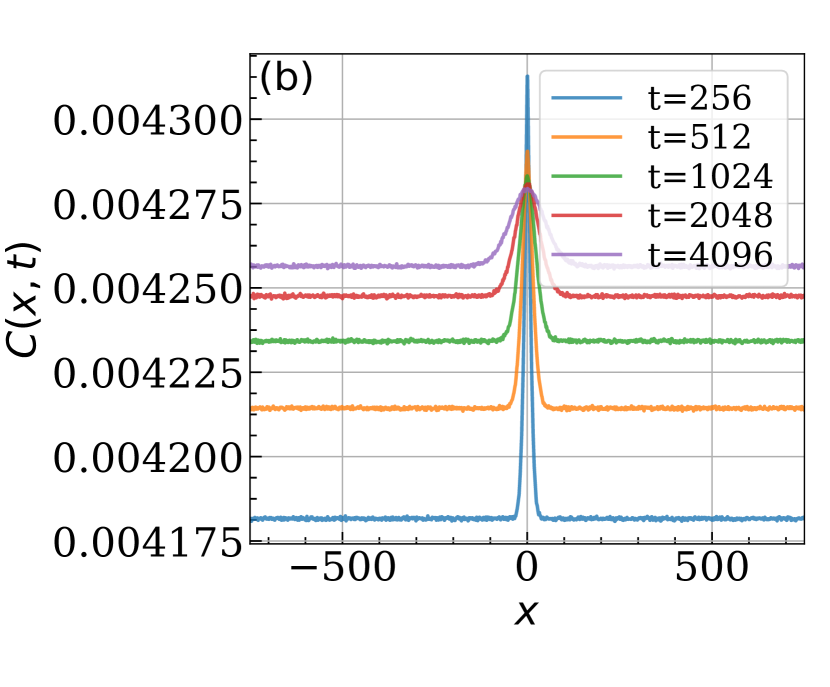
Figure 5: (a) Plot of prethermal temperature at time $t_{w}$ to time $t$ as defined by $T(t)/T(t_{w})=\sum_{i}p_{i}(t)^{2}/\sum_{i}p_{i}(\tau_{w})^{2}$. For smaller values $K$, the heating is suppressed for a larger timescale, while for $K=0.24$ the heating sets in early causing the prethermal temporal window to shrink. (b) Unsubtracted correlations of kinetic energy $\langle{p_{i}^{2}(t)}{p_{j}^{2}(t_{w})}\rangle$ for $K=0.14$ are shown. We find the drift in time for the correlation functions. With the deterministic part $\langle{p_{i}^{2}(t)}\rangle\langle{p_{j}^{2}(t_{w})}\rangle$ subtracted, this drift goes to zero. This is in contrast to an equilibrium system, where the average is independent of time.

In the prethermal regime, a typical fluctuation spreads in space and time diffusively in the system. A proper diffusive scaling makes the spatio-temporal correlation function collapse to a Gaussian distribution, with two free parameters: the amplitude of the Gaussian and the diffusion coefficient of the Gaussian. The mathematical form of the correlation for a given value of $K$ is thus given by $C(x,t)\sim A_{K}t^{-1/2}f\big{(}xt^{-1/2}\big{)}$, with $f(y)=e^{-y^{2}/2D}/\sqrt{2\pi D}$ where $A_{K}$ and $D$ are the amplitude and the diffusion coefficient for the Gaussian distribution. However, extracting the dependence of the diffusion coefficient on driving frequency is numerically more difficult due to both finite time and finite size effects. Our analysis suggests that the diffusion coefficient is very weakly dependent on the driving frequency of the system. We plot the dependence in Fig. 6 where it looks like the typical $K$ dependence might be due to finite time effect.

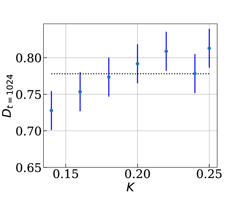
Figure 6: The diffusion constant extracted by fitting the scaled dynamical correlations at time $t=1024$. The diffusion constant looks very slowly changing with $0.15<K<0.23$ but appears to be saturating around $0.775$. Note that for smaller $K$, time $1024$ is not large enough for the hydrodynamical scale, hence the results are severely affected by the finite time effect.

Appendix C Solution of the hydrodynamic equation

We now discuss the hydrodynamic picture of the driven system at times when the prethermal description is valid, i.e. at times much less than the marginalized time ($t<<t_{m}$)Rajak et al. (2018, 2019). This time scales with the driving frequency as $t_{m}\sim e^{3/K}$. The emergent fluctuations in the prethermal region can be represented by the diffusion equation

$$\partial_{t}u(x,t)\approxeq\frac{D}{2}\partial_{x}^{2}u(x,t)+B\partial_{x}\zeta(x,t)$$ (21)

where $u(x,t)=\frac{1}{2}\left(p^{2}(x,t)-\langle p^{2}(x,t)\rangle\right)$ such that $\langle u(x,t)\rangle\neq\langle u(x,t^{\prime})\rangle$. The averages are taken over a GGE at temperature $T^{*}$. In the prethermal region, the temperature increment is exponentially suppressed, resulting in an effective hydrodynamic description of the system. The noise $\zeta(x,t)$ of strength $B$ is delta correlated in space and time $\langle\zeta(x,t)\zeta(x^{\prime},t^{\prime})\rangle=\delta_{xx^{\prime}}\delta(t-t^{\prime})$. The derivative under the noise term is due to the almost conserved nature of the total energy of the system in the prethermal phase. There could be an additional exponentially small forcing term present in the diffusion equation. This term might drive the system out of prethermal phase at later time.

One can solve the above equation by Fourier transform $u(x,t)=\frac{1}{\sqrt{2\pi}}\int dke^{ikx}u_{k}(t)$ and $\zeta(x,t)=\frac{1}{\sqrt{2\pi}}\int dke^{ikx}\zeta_{k}(t)$. The equation becomes

$$\partial_{t}u_{k}(t)=-\frac{Dk^{2}}{2}u_{k}(t)+{i\mkern 1.0mu}kB\zeta_{k}(t),$$ (22)

where the noise correlations are now given as $\langle\zeta_{k}(t)\zeta_{k^{\prime}}(t^{\prime})\rangle=\delta_{kk^{\prime}}\delta(t-t^{\prime})$. The general solution to the above equation is given as,

$$u_{k}(t)=e^{-\frac{Dk^{2}}{2}t}u_{k}(0)+{i\mkern 1.0mu}k\int_{-\infty}^{t}dt^{\prime}e^{-\frac{Dk^{2}}{2}(t-t^{\prime})}B\zeta_{k}(t^{\prime})$$ (23)

From this solution the correlation function is obtained by multiplying this equation by $u_{k}(\tau_{w})$ and taking an equilibrium average to get,

$$\langle u_{k}(t)u_{k^{\prime}}(\tau_{w})\rangle=e^{-\frac{Dk^{2}}{2}(t-\tau_{w})}\langle u_{k}(\tau_{w})^{2}\rangle\delta_{k,k^{\prime}}$$ (24)

The average is over the prethermal state. As shown in Ref. Rajak et al., 2019 that the different modes (away from $k=0$) in the prethermal state are independent and acquires marginal localization independent on the wave numbers. Following an inverse Fourier transform, we get the spatio-temporal correlation functions as,

$$C(x,t-\tau_{w}) = \frac{1}{\sqrt{2\pi}}\int dke^{-{i\mkern 1.0mu}kx}e^{-\frac{Dk^{2}}{2}(t-\tau_{w})}\langle u_{k}(\tau_{w})^{2}\rangle$$ (25)

$$= \frac{\langle u(\tau_{w})^{2}\rangle}{\sqrt{2\pi D(t-\tau_{w})}}e^{-x^{2}/(2D(t-\tau_{w}))}$$

Fluctuation Dissipation in the large time limit Eq. 23, the first part vanishes and the memory of the initial condition vanishes. One can obtain

$$u_{k}(t)=\lim_{t\to\infty}{i\mkern 1.0mu}k\int_{-\infty}^{t}dt^{\prime}e^{-\frac{Dk^{2}}{2}(t-t^{\prime})}B\zeta_{k}(t^{\prime})$$ (26)

Squaring both sides and using the correlations of the noise, we have

$$\langle u_{k}(t)^{2}\rangle = -k^{2}\int_{-\infty}^{t}dt^{\prime\prime}\int_{-\infty}^{t}dt^{\prime}e^{-\frac{Dk^{2}}{2}(t-t^{\prime})}e^{-\frac{Dk^{2}}{2}(t-t^{\prime\prime})}$$ (27)

$$\times B^{2}\langle\zeta_{k}(t^{\prime})\zeta_{k}(t^{\prime\prime})\rangle$$

$$=-k^{2}\int_{-\infty}^{t}dt^{\prime\prime}\int_{-\infty}^{t}dt^{\prime}e^{-\frac{Dk^{2}}{2}(t-t^{\prime})}e^{-\frac{Dk^{2}}{2}(t-t^{\prime\prime})}$$

$$\times B^{2}\delta(t^{\prime}-t^{\prime\prime})$$

$$\overset{t\to\infty}{=}-k^{2}\int_{-\infty}^{t}dt^{\prime}e^{-\frac{Dk^{2}}{2}2(t-t^{\prime})}B^{2}$$

$$= ~{}B^{2}/D$$

where we assumed that at large time $t$, the system is approximately in the prethermal state defined by the GGE temperature $T^{*}$. The fluctuations of average in the prethermal region is $\langle u_{k}^{2}\rangle_{T^{*}}=\langle u^{2}\rangle_{T^{*}}=C$. Note that this relation is exact in the case when the system is static. In the prethermal region, this relation is approximately correct to a large timescale, before the heating mechanism takes place. This yields $DC\approxeq B^{2}$, which we refer to as the approximate fluctuation dissipation relation (AFDR) in prethermal phase. The correction to this is of the order of $1/k^{2}$, if we consider a delta correlated noisy forcing term. In the large wavelength limit, i.e. at short but enough coarse-grained space, this contribution goes away and the result approximately holds true.

In the driven system, all the oscillators individually get kicked periodically in time. The kick inflicts extra energy to the system that gets dissipated in the system eventually. This results in an effective time averaged current in the system $j\sim K\langle\nabla_{x}V^{\prime}(x)\rangle$. This makes the noise coefficient $B\sim K$. Along with the AFDR, this give that $D\sim K^{0}$.

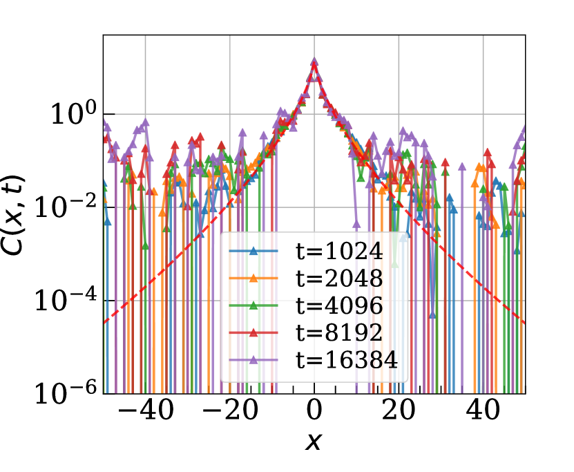
Figure 7: Plot of the correlations in the semi-log scale for the crossover region with $K=0.7$. The same quantity is plotted in Fig. 3 in linear scale with stretched exponential fit around the disturbance core at $x=0$. We here emphasize on the accuracy of stretched exponential fit by redrawing it in the semi-log scale.

Appendix D Stretched exponential correlations in crossover region

We here discuss the intermediate crossover region, where the correlations are exponentially localized in real space with no time dynamics. As mentioned in the main text and Fig. 3 of the main text, we find that the stretched exponential description of the system is in good agreement when the correlation are measured in the close vicinity of fluctuation core $x\ll|N/2|$ where $N$ is the system size $[-N/2:N/2]$. We redraw the same quantity in semi-log scale with stretched exponential fit in Fig. 7. We can observe that even in logarithmic scale, the stretched exponential fit of the correlator is appropriate around the disturbance core $x=0$. This indicates the robustness of the stretched exponential fit of the spatio-temporal correlator in the crossover regime. One can clearly notice that correlation becomes heavily fluctuating with time and space. The timescale of this crossover decrease with time, and in infinitely large time limit, the correlations become spatially delta correlated as shown in Fig. 4 of the main text.

Appendix E Frozen correlation in heating region

We here discuss the analytical form of the correlation in the heating region that is derived with the help of the assumptions as given in Eq. (7). We start by using Eq. (2), the momentum of $i$-th rotor at any time $t$ can be written as

$$p_{i}(t)=p_{i}(0)-K\sum_{n=0}^{t-1}[\sin(r_{i}(n))-\sin(r_{i-1}(n))],$$ (28)

where $p_{i}(0)$ is the momentum of the $i$-th rotor at time $t=0$. In our numerical calculations, we have assumed the initial momenta of all the rotors to be zero. The momentum of a rotor at any stroboscopic time $t$ depends on the initial momentum, and the values of angles of that rotor and its nearest neighbors at the earlier time. We below derive the correlator assuming the fact that rotors are always uncorrelated from the very beginning of the dynamics. This allows us to write the summation over time starting from $n=0$ as described below. However, we know from the numerical analysis that driven system requires some time to enter into the heating region. Hence we note that the independent rotor approximation works better to explain the numerical outcomes for higher values of $K$ as the driven system enters into the heating region quite early.

Now the first term of the kinetic energy fluctuation correlator with $t>t_{w}$ can be calculated in the heating regime as follows

$$\langle p_{i}^{2}(t)p_{j}^{2}(t_{w})\rangle=K^{4}\Bigg{\langle}\sum_{n,n^{\prime}=0}^{t-1}\sum_{m,m^{\prime}=0}^{t_{w}-1}\Bigg{[}[\sin(r_{i}(n))-\sin(r_{i-1}(n))]$$

$$\times[\sin(r_{i}(n^{\prime}))-\sin(r_{i-1}(n^{\prime}))]\times[\sin(r_{j}(m))-\sin(r_{j-1}(m))]$$

$$\times[\sin(r_{j}(m^{\prime}))-\sin(r_{j-1}(m^{\prime}))]\Bigg{]}\Bigg{\rangle}$$

$$=K^{4}\Bigg{\langle}\sum_{n,n^{\prime}=0}^{t-1}\sum_{m,m^{\prime}=0}^{t_{w}-1}\Bigg{[}\Big{[}\sin(r_{i}(n))\sin(r_{i}(n^{\prime}))$$

$$+\sin(r_{i-1}(n))\sin(r_{i-1}(n^{\prime}))$$

$$-\sin(r_{i}(n))\sin(r_{i-1}(n^{\prime}))-\sin(r_{i-1}(n))\sin(r_{i}(n^{\prime}))\Big{]}$$

$$\times\Big{[}\sin(r_{j}(m))\sin(r_{j}(m^{\prime}))+\sin(r_{j-1}(m))\sin(r_{j-1}(m^{\prime}))$$

$$-\sin(r_{j}(m))\sin(r_{j-1}(m^{\prime}))-\sin(r_{j-1}(m))\sin(r_{j}(m^{\prime}))\Big{]}\Bigg{]}\Bigg{\rangle}$$

$$=K^{4}\sum_{n,n^{\prime}=0}^{t-1}\sum_{m,m^{\prime}=0}^{t_{w}-1}\Big{(}2~{}\delta_{n,m}\delta_{n^{\prime},m^{\prime}}\delta_{i,j}+\frac{1}{2}~{}\delta_{n,m}\delta_{n^{\prime},m^{\prime}}\delta_{i,j+1}$$

$$+\frac{1}{2}~{}\delta_{n,m}\delta_{n^{\prime},m^{\prime}}\delta_{i,j-1}+\delta_{n,n^{\prime}}\delta_{m,m^{\prime}}\delta_{i,i}\delta_{j,j}$$

$$+\frac{3}{4}~{}\delta_{n,n^{\prime}}\delta_{m,m^{\prime}}\delta_{m,n}\delta_{i,i}\delta_{j,j}\delta_{i,j}$$

$$+\frac{3}{8}~{}\delta_{n,n^{\prime}}\delta_{m,m^{\prime}}\delta_{m,n}\delta_{i,i}\delta_{j,j}\delta_{i,j+1}$$

$$+\frac{3}{8}~{}\delta_{n,n^{\prime}}\delta_{m,m^{\prime}}\delta_{m,n}\delta_{i,i}\delta_{j,j}\delta_{i,j-1}\Big{)}$$

$$=K^{4}\Big{(}2~{}t_{w}^{2}\delta_{i,j}+\frac{3}{4}t_{w}\delta_{i,j}+\frac{1}{2}~{}t_{w}^{2}\delta_{i,j+1}+\frac{3}{8}~{}t_{w}\delta_{i,j+1}$$

$$+\frac{1}{2}~{}t_{w}^{2}\delta_{i,j-1}+\frac{3}{8}~{}t_{w}\delta_{i,j-1}+tt_{w}\delta_{i,i}\delta_{j,j}\Big{)}.$$ (29)

Here we use the fact that $\delta_{i,j}\delta_{i^{\prime},j}=\delta_{i,j}\delta_{i,j^{\prime}}=0$. The second part $\langle p_{i}^{2}(t)\rangle\langle p_{j}^{2}(t_{w})\rangle$ now looks like

$$\langle p_{i}^{2}(t)\rangle\langle p_{j}^{2}(t_{w})\rangle=K^{4}\Bigg{\langle}\sum_{n,n^{\prime}=0}^{t-1}[\sin(r_{i}(n))-\sin(r_{i-1}(n))]$$

$$\times[\sin(r_{i}(n^{\prime}))-\sin(r_{i-1}(n^{\prime}))]\Bigg{\rangle}$$

$$\times\Bigg{\langle}\sum_{m,m^{\prime}=0}^{t_{w}-1}[\sin(r_{j}(m))-\sin(r_{j-1}(m))]$$

$$\times[\sin(r_{j}(m^{\prime}))-\sin(r_{j-1}(m^{\prime}))]\Bigg{\rangle}$$

$$=K^{4}tt_{w}\delta_{i,i}\delta_{j,j}$$ (30)

This leads to write the kinetic energy correlator as

$$C(i,j,t,t_{w})=\frac{1}{4}[\langle p_{i}^{2}(t)p_{j}^{2}(t_{w})\rangle-\langle p_{i}^{2}(t)\rangle\langle p_{j}^{2}(t_{w})\rangle]$$

$$=K^{4}\Big{(}\frac{t_{w}^{2}}{2}\delta_{i,j}+\frac{t_{w}^{2}}{8}\delta_{i,j+1}+\frac{t_{w}^{2}}{8}\delta_{i,j-1}\Big{)}+O(t_{w}).$$ (31)

References

- Shirley (1965) J. H. Shirley, Phys. Rev. 138, B979 (1965).
- Dunlap and Kenkre (1986) D. H. Dunlap and V. M. Kenkre, Phys. Rev. B 34, 3625 (1986).
- Grifoni and Hänggi (1998) M. Grifoni and P. Hänggi, Physics Reports 304, 229 (1998).
- Goldman and Dalibard (2014a) N. Goldman and J. Dalibard, Phys. Rev. X 4, 031027 (2014a).
- Eckardt (2017) A. Eckardt, Review of Modern Physics 89, 011004 (2017).
- Bukov et al. (2015a) M. Bukov, L. D’Alessio, and A. Polkovnikov, Advances in Physics 64, 139 (2015a).
- Wang et al. (2013) Y. H. Wang, H. Steinberg, P. Jarillo-Herrero, and N. Gedik, Science 342, 453 (2013).
- Rechtsman et al. (2013) M. C. Rechtsman, J. M. Zeuner, Y. Plotnik, Y. Lumer, D. Podolsky, F. Dreisow, S. Nolte, M. Segev, and A. Szameit, Nature 496, 196 (2013).
- Peng et al. (2016) Y.-G. Peng, C.-Z. Qin, D. Zhao, Y. X. Shen, X.-Y. Xu, M. Bao, H. Jia, and X.-F. Zhu, Nature Communications 7, 13368 (2016).
- Fleury et al. (2016) R. Fleury, A. B. Khanikaev, and A. Alu, Nature communications 7, 11744 (2016).
- Maczewsky et al. (2017) L. J. Maczewsky, J. M. Zeuner, S. Nolte, and A. Szameit, Nature communications 8, 13756 (2017).
- Kayanuma and Saito (2008) Y. Kayanuma and K. Saito, Phys. Rev. A 77, 010101 (2008).
- Nag et al. (2014) T. Nag, S. Roy, A. Dutta, and D. Sen, Phys. Rev. B 89, 165425 (2014).
- Nag et al. (2015) T. Nag, D. Sen, and A. Dutta, Phys. Rev. A 91, 063607 (2015).
- D’Alessio and Polkovnikov (2013) L. D’Alessio and A. Polkovnikov, Annals of Physics 333, 19 (2013).
- D’Alessio and Rigol (2014) L. D’Alessio and M. Rigol, Physical Review X 4, 041048 (2014).
- Ponte et al. (2015a) P. Ponte, A. Chandran, Z. Papić, and D. A. Abanin, Annals of Physics 353, 196 (2015a).
- Ponte et al. (2015b) P. Ponte, Z. Papić, F. m. c. Huveneers, and D. A. Abanin, Phys. Rev. Lett. 114, 140401 (2015b).
- Lazarides et al. (2015) A. Lazarides, A. Das, and R. Moessner, Physical Review Letters 115, 030402 (2015).
- Zhang et al. (2016) L. Zhang, V. Khemani, and D. A. Huse, Phys. Rev. B 94, 224202 (2016).
- Eckardt et al. (2005) A. Eckardt, C. Weiss, and M. Holthaus, Physical Review Letters 95, 260404 (2005).
- Zenesini et al. (2009) A. Zenesini, H. Lignier, D. Ciampini, O. Morsch, and E. Arimondo, Phys. Rev. Lett. 102, 100403 (2009).
- Oka and Aoki (2009) T. Oka and H. Aoki, Physical Review B 79, 081406 (2009).
- Kitagawa et al. (2011) T. Kitagawa, T. Oka, A. Brataas, L. Fu, and E. Demler, Physical Review B 84, 235108 (2011).
- Lindner et al. (2011) N. H. Lindner, G. Refael, and V. Galitski, Nature Physics 7, 490 (2011).
- Rudner et al. (2013) M. S. Rudner, N. H. Lindner, E. Berg, and M. Levin, Physical Review X 3, 031005 (2013).
- Rodriguez-Vega et al. (2019) M. Rodriguez-Vega, A. Kumar, and B. Seradjeh, Phys. Rev. B 100, 085138 (2019).
- Seshadri et al. (2019) R. Seshadri, A. Dutta, and D. Sen, Phys. Rev. B 100, 115403 (2019).
- Nag et al. (2019a) T. Nag, V. Juričić, and B. Roy, Phys. Rev. Research 1, 032045 (2019a).
- Nag et al. (2020) T. Nag, V. Juricic, and B. Roy, arXiv preprint arXiv:2009.10719 (2020).
- Nag and Roy (2020) T. Nag and B. Roy, arXiv preprint arXiv:2010.11952 (2020).
- Ghosh et al. (2021a) A. K. Ghosh, T. Nag, and A. Saha, Phys. Rev. B 103, 045424 (2021a).
- Ghosh et al. (2021b) A. K. Ghosh, T. Nag, and A. Saha, Phys. Rev. B 103, 085413 (2021b).
- Else et al. (2016) D. V. Else, B. Bauer, and C. Nayak, Physical Review Letters 117, 090402 (2016).
- Khemani et al. (2016) V. Khemani, A. Lazarides, R. Moessner, and S. L. Sondhi, Physical Review Letters 116, 250401 (2016).
- Zhang et al. (2017) J. Zhang, P. Hess, A. Kyprianidis, P. Becker, A. Lee, J. Smith, G. Pagano, I.-D. Potirniche, A. C. Potter, A. Vishwanath, et al., Nature 543, 217 (2017).
- Yao et al. (2017) N. Y. Yao, A. C. Potter, I.-D. Potirniche, and A. Vishwanath, Physical Review Letters 118, 030401 (2017).
- Faisal and Kamiński (1997) F. H. M. Faisal and J. Z. Kamiński, Phys. Rev. A 56, 748 (1997).
- Nag et al. (2019b) T. Nag, R.-J. Slager, T. Higuchi, and T. Oka, Phys. Rev. B 100, 134301 (2019b).
- Ikeda et al. (2018) T. N. Ikeda, K. Chinzei, and H. Tsunetsugu, Phys. Rev. A 98, 063426 (2018).
- Neufeld et al. (2019) O. Neufeld, D. Podolsky, and O. Cohen, Nature communications 10, 1 (2019).
- Bilitewski and Cooper (2015) T. Bilitewski and N. R. Cooper, Phys. Rev. A 91, 033601 (2015).
- Reitter et al. (2017) M. Reitter, J. Näger, K. Wintersperger, C. Sträter, I. Bloch, A. Eckardt, and U. Schneider, Phys. Rev. Lett. 119, 200402 (2017).
- Boulier et al. (2019) T. Boulier, J. Maslek, M. Bukov, C. Bracamontes, E. Magnan, S. Lellouch, E. Demler, N. Goldman, and J. V. Porto, Phys. Rev. X 9, 011047 (2019).
- Moessner and Sondhi (2017) R. Moessner and S. L. Sondhi, Nature Physics 13, 424 (2017).
- Luitz et al. (2017) D. J. Luitz, Y. B. Lev, and A. Lazarides, SciPost Phys. 3, 029 (2017).
- Seetharam et al. (2018) K. Seetharam, P. Titum, M. Kolodrubetz, and G. Refael, Phys. Rev. B 97, 014311 (2018).
- Prosen (1998) T. c. v. Prosen, Phys. Rev. Lett. 80, 1808 (1998).
- Haldar et al. (2018) A. Haldar, R. Moessner, and A. Das, Phys. Rev. B 97, 245122 (2018).
- Russomanno et al. (2012) A. Russomanno, A. Silva, and G. E. Santoro, Physical Review Letters 109, 257201 (2012).
- Gritsev and Polkovnikov (2017) V. Gritsev and A. Polkovnikov, SciPost Phys 2, 021 (2017).
- Choudhury and Mueller (2014) S. Choudhury and E. J. Mueller, Physical Review A 90, 013621 (2014).
- Bukov et al. (2015b) M. Bukov, S. Gopalakrishnan, M. Knap, and E. Demler, Physical Review Letters 115, 205301 (2015b).
- Citro et al. (2015) R. Citro, E. G. Dalla Torre, L. D’Alessio, A. Polkovnikov, M. Babadi, T. Oka, and E. Demler, Annals of Physics 360, 694 (2015).
- Mori (2015) T. Mori, Phys. Rev. A 91, 020101 (2015).
- Chandran and Sondhi (2016) A. Chandran and S. L. Sondhi, Physical Review B 93, 174305 (2016).
- Canovi et al. (2016) E. Canovi, M. Kollar, and M. Eckstein, Physical Review E 93, 012130 (2016).
- Mori et al. (2016) T. Mori, T. Kuwahara, and K. Saito, Physical review letters 116, 120401 (2016).
- Lellouch et al. (2017) S. Lellouch, M. Bukov, E. Demler, and N. Goldman, Physical Review X 7, 021015 (2017).
- Weidinger and Knap (2017) S. A. Weidinger and M. Knap, Scientific Reports 7, 45382 (2017).
- Abanin et al. (2017a) D. A. Abanin, W. De Roeck, W. W. Ho, and F. Huveneers, Physical Review B 95, 014112 (2017a).
- Else et al. (2017) D. V. Else, B. Bauer, and C. Nayak, Physical Review X 7, 011026 (2017).
- Zeng and Sheng (2017) T.-S. Zeng and D. Sheng, Physical Review B 96, 094202 (2017).
- Peronaci et al. (2018) F. Peronaci, M. Schiró, and O. Parcollet, Phys. Rev. Lett. 120, 197601 (2018).
- Rajak et al. (2018) A. Rajak, R. Citro, and E. G. Dalla Torre, Journal of Physics A: Mathematical and Theoretical 51, 465001 (2018).
- Mori (2018) T. Mori, Phys. Rev. B 98, 104303 (2018).
- Howell et al. (2019) O. Howell, P. Weinberg, D. Sels, A. Polkovnikov, and M. Bukov, Phys. Rev. Lett. 122, 010602 (2019).
- Rajak et al. (2019) A. Rajak, I. Dana, and E. G. Dalla Torre, Physical Review B 100, 100302 (2019).
- Abanin et al. (2017b) D. Abanin, W. De Roeck, W. W. Ho, and F. Huveneers, Communications in Mathematical Physics 354, 809 (2017b).
- Torre (2020) E. G. D. Torre, arXiv preprint arXiv:2005.07207 (2020).
- Hodson and Jarzynski (2021) W. Hodson and C. Jarzynski, Phys. Rev. Research 3, 013219 (2021).
- Castro-Alvaredo et al. (2016) O. A. Castro-Alvaredo, B. Doyon, and T. Yoshimura, Phys. Rev. X 6, 041065 (2016).
- Mori et al. (2018) T. Mori, T. N. Ikeda, E. Kaminishi, and M. Ueda, Journal of Physics B: Atomic, Molecular and Optical Physics 51, 112001 (2018).
- Deutsch (2018) J. M. Deutsch, Reports on Progress in Physics 81, 082001 (2018).
- Das and Dhar (2014) S. G. Das and A. Dhar, arXiv preprint arXiv:1411.5247 (2014).
- Mendl and Spohn (2013) C. B. Mendl and H. Spohn, Phys. Rev. Lett. 111, 230601 (2013).
- Mendl and Spohn (2014) C. B. Mendl and H. Spohn, Phys. Rev. E 90, 012147 (2014).
- Spohn (2014a) H. Spohn, Journal of Statistical Physics 154, 1191 (2014a).
- Mendl and Spohn (2015) C. B. Mendl and H. Spohn, Journal of Statistical Mechanics: Theory and Experiment 2015, P03007 (2015).
- Kundu and Dhar (2016) A. Kundu and A. Dhar, Phys. Rev. E 94, 062130 (2016).
- Dhar et al. (2019) A. Dhar, A. Kundu, J. L. Lebowitz, and J. A. Scaramazza, Journal of Statistical Physics 175, 1298 (2019).
- Doyon (2019) B. Doyon, Journal of Mathematical Physics 60, 073302 (2019).
- Das et al. (2020) A. Das, K. Damle, A. Dhar, D. A. Huse, M. Kulkarni, C. B. Mendl, and H. Spohn, Journal of Statistical Physics 180, 238 (2020).
- Das et al. (2014) S. G. Das, A. Dhar, K. Saito, C. B. Mendl, and H. Spohn, Phys. Rev. E 90, 012124 (2014).
- Bastianello et al. (2018) A. Bastianello, B. Doyon, G. Watts, and T. Yoshimura, SciPost Phys 4, 33 (2018).
- De Nardis et al. (2018) J. De Nardis, D. Bernard, and B. Doyon, Phys. Rev. Lett. 121, 160603 (2018).
- Spohn (2020) H. Spohn, Journal of Physics A: Mathematical and Theoretical 53, 265004 (2020).
- Cataliotti et al. (2001) F. Cataliotti, S. Burger, C. Fort, P. Maddaloni, F. Minardi, A. Trombettoni, A. Smerzi, and M. Inguscio, Science 293, 843 (2001).
- Cheneau et al. (2012) M. Cheneau, P. Barmettler, D. Poletti, M. Endres, P. Schauß, T. Fukuhara, C. Gross, I. Bloch, C. Kollath, and S. Kuhr, Nature 481, 484 (2012).
- Goldman and Dalibard (2014b) N. Goldman and J. Dalibard, Physical review X 4, 031027 (2014b).
- Messer et al. (2018) M. Messer, K. Sandholzer, F. Görg, J. Minguzzi, R. Desbuquois, and T. Esslinger, Phys. Rev. Lett. 121, 233603 (2018).
- Rubio-Abadal et al. (2020) A. Rubio-Abadal, M. Ippoliti, S. Hollerith, D. Wei, J. Rui, S. L. Sondhi, V. Khemani, C. Gross, and I. Bloch, Phys. Rev. X 10, 021044 (2020).
- Kaneko and Konishi (1989) K. Kaneko and T. Konishi, Physical Review A 40, 6130 (1989).
- Konishi and Kaneko (1990) T. Konishi and K. Kaneko, Journal of Physics A: Mathematical and General 23, L715 (1990).
- Falcioni et al. (1991) M. Falcioni, U. M. B. Marconi, and A. Vulpiani, Physical Review A 44, 2263 (1991).
- Chirikov and Vecheslavov (1993) B. Chirikov and V. Vecheslavov, Journal of statistical physics 71, 243 (1993).
- Chirikov and Vecheslavov (1997) B. Chirikov and V. Vecheslavov, Journal of Experimental and Theoretical Physics 85, 616 (1997).
- Mulansky et al. (2011) M. Mulansky, K. Ahnert, A. Pikovsky, and D. L. Shepelyansky, Journal of Statistical Physics 145, 1256 (2011).
- Rajak and Dana (2020) A. Rajak and I. Dana, Physical Review E 102, 062120 (2020).
- Lepri (2016) S. Lepri, Thermal transport in low dimensions: from statistical physics to nanoscale heat transfer (Springer (2016)).
- Dhar (2008) A. Dhar, Advances in Physics 57, 457 (2008).
- Khasseh et al. (2019) R. Khasseh, R. Fazio, S. Ruffo, and A. Russomanno, Phys. Rev. Lett. 123, 184301 (2019).
- Spohn (2014b) H. Spohn, arXiv preprint arXiv:1411.3907 (2014b).
- Spohn (2016) H. Spohn, arXiv preprint arXiv:1601.00499 (2016).
- Dhar et al. (2021) A. Dhar, A. Kundu, and K. Saito, Chaos, Solitons & Fractals 144, 110618 (2021).
- Ye et al. (2020) B. Ye, F. Machado, C. D. White, R. S. K. Mong, and N. Y. Yao, Phys. Rev. Lett. 125, 030601 (2020).
- (107) We compute other fluctuation correlation such as, unequal (equal) space and equal (unequal) time correlation, that also shows distinct features in the different dynamic phases (in preparation).
- Lerose et al. (2019) A. Lerose, B. Žunkovič, A. Silva, and A. Gambassi, Phys. Rev. B 99, 121112 (2019).
- Saha et al. (2019) M. Saha, S. K. Maiti, and A. Purkayastha, Phys. Rev. B 100, 174201 (2019).
- De Tomasi (2019) G. De Tomasi, Phys. Rev. B 99, 054204 (2019).
- Nag and Garg (2019) S. Nag and A. Garg, Phys. Rev. B 99, 224203 (2019).
- Modak and Nag (2020a) R. Modak and T. Nag, Phys. Rev. Research 2, 012074 (2020a).
- Modak and Nag (2020b) R. Modak and T. Nag, Phys. Rev. E 101, 052108 (2020b).