Random Graphs with Prescribed $K$-Core Sequences:
A New Null Model for Network Analysis

Abstract.

In the analysis of large-scale network data, a fundamental operation is the comparison of observed phenomena to the predictions provided by null models: when we find an interesting structure in a family of real networks, it is important to ask whether this structure is also likely to arise in random networks with similar characteristics to the real ones. A long-standing challenge in network analysis has been the relative scarcity of reasonable null models for networks; arguably the most common such model has been the configuration model, which starts with a graph $G$ and produces a random graph with the same node degrees as $G$. This leads to a very weak form of null model, since fixing the node degrees does not preserve many of the crucial properties of the network, including the structure of its subgraphs.

Guided by this challenge, we propose a new family of network null models that operate on the $k$-core decomposition. For a graph $G$, the $k$-core is its maximal subgraph of minimum degree $k$; and the core number of a node $v$ in $G$ is the largest $k$ such that $v$ belongs to the $k$-core of $G$. We provide the first efficient sampling algorithm to solve the following basic combinatorial problem: given a graph $G$, produce a random graph sampled nearly uniformly from among all graphs with the same sequence of core numbers as $G$. This opens the opportunity to compare observed networks $G$ with random graphs that exhibit the same core numbers, a comparison that preserves aspects of the structure of $G$ that are not captured by more local measures like the degree sequence. We illustrate the power of this core-based null model on some fundamental tasks in network analysis, including the enumeration of networks motifs.

1. Introduction

Random graphs have long played a central role in the area of network analysis, and one of their crucial uses has been as null models: a way of producing families of synthetic graphs that match observed network data on specific basic properties. Armed with effective null models, we can take an observed network phenomenon and ask whether a random graph with similar characteristics would exhibit the same phenomenon or not.

This comparison to random-graph baselines is an essential strategy, but of course the challenge is to define what we mean by a random graph “with similar characteristics.” In these types of analyses, a widely-used null model — arguably the ubiquitous default — is the configuration model: given an observed network $G$, it generates random graphs sampled uniformly at random from among all graphs with the same degree sequence as $G$. The configuration model has provided a powerful way of asserting that observed properties of real networks are not simply a consequence of the node degrees, in that they would be unlikely in a random graph with the same degree sequence (newman2001random, ; fosdick2018configuring, ).

Despite the widespread use of the configuration model, it is well-understood to be an extremely weak null model, particularly for any question involving local rather than global structure. In particular, a random graph with a given degree sequence will typically have very little non-trivial local structure in the neighborhood of any given node $v$, and very little non-trivial community structure. Thus, real networks will almost always look very different from the predictions of a random draw from the configuration model on any question involving structures like local motifs or dense communities; and these are some of the main questions for which people seek out random graphs as baselines.

Given these limitations of the configuration model, researchers have sought other null models in which we sample uniformly or near-uniformly over different families of graphs defined by characteristics of a given real network. Stanton and Pinar, for example, show how to sample from graphs that match an observed network $G$ not just in its degree sequence but in the pairs of degrees $(d_{i},d_{j})$ arising from the edges $(i,j)$ of $G$ (stanton2012constructing, ). This increases the specificity of the null model, but it continues to lack non-trivial local or community structure. An interesting recent step toward null models designed to exhibit local structure was taken by Orsini et al. (orsini2015quantifying, ), who generalized and put into practice the $dK$-series hierarchy of random graph models (mahadevan2006systematic, ), where the lowest levels match the degree sequence or degree correlations and higher-levels — the 2.1-series and 2.5-series — also match statistics on triangles such as the average clustering coefficient or the sequence of clustering coefficients. This approach comes with the obstacle, however, there are not any practical algorithms for uniformly sampling from these subsequent levels that match more than just degrees and pairs of degrees; as a result, while they constitute valuable heuristics, they are not designed to provide guarantees on near-uniform sampling from the associated family of graphs.

Thus, a basic question has remained: given an observed graph $G$, can we construct a null model by sampling from a family of graphs matching characteristics of $G$ in such a way that the resulting random samples exhibit non-trivially rich local structure and community structure?

The present work: A null model based on the $k$-core.

In this paper, we provide a new approach to this question, by showing how to uniformly sample from graphs that match $G$ in its k-core properties. The resulting samples provide random-graph baselines with richer graph-theoretic structure than the configuration model, and we show that they can lead to potentially different conclusions when employed as null models.

To formulate our approach, we begin with some basic definitions. Given a graph $G$ and a number $k$, the $k$-core of $G$ is the (unique) maximal subgraph of $G$ in which every node has degree at least $k$; it can be found efficiently by iteratively deleting nodes of degree strictly less than $k$ in $G$. (For sufficiently large $k$, $G$ will have no subgraph of minimum degree $k$, and hence the $k$-core of $G$ for these large $k$ will be the empty graph.) Building on this definition, we say that the core-value $c_{v}$ of a node $v$ is the largest $k$ such that $v$ belongs to the $k$-core of $G$.

A long line of work in network analysis has shown that successive $k$-cores of $G$, for $k=0,1,2,...$, provides considerable information about the local structure of $G$, including the regions where it exhibits denser connectivity (dorogovtsev2006k, ; carmi2007model, ; shin2016corescope, ; laishram2018measuring, ; malliaros2020core, ). This information is equivalently captured by the sequence of core-values $c_{1}\geq c_{2}\geq\cdots\geq c_{n}$ of the $n$ nodes of $G$.

Given this, we ask the following question: by analogy with the configuration model, which samples uniformly from all graphs matching the degree sequence of $G$, can we sample uniformly (or near-uniformly) from all graphs matching the sequence of core numbers of $G$? We could do this in theory by brute-force rejection sampling, so our goal is to develop reasonable algorithms for generating such samples. This type of sampler would provide a genuinely new type of null model, by producing random graphs that match an observed $G$ on richer forms of structure than the degree sequence.

Sampling a random graph with a given core-value sequence.

We answer this question affirmatively, by providing a method for near-uniform sampling from graphs with a given core-value sequence. We provide an overview of our strategy here, and give details in the subsequent sections.

Our basic approach is to define a Markov chain whose state space is the set of all graphs with the given core-value sequence, and whose transitions are a set of graph transformations that preserve the core-values. The crux of the method, and the heart of our analysis, is the definition of a sufficiently rich set of local transformations such that sequences of these transformations, composed together, are able to transform a starting graph $G_{0}$ into any other graph with the same core-value sequence. Applying random transformation to an underlying graph thus produces a Markov chain on the set of all graphs of a given core-value sequence. Our results establish that the Markov chain is strongly connected; and by adding appropriate probabilities on the “identity transformation” that leaves the graph unchanged, we can also ensure that the chain is aperiodic and has a uniform stationary distribution. Thus, by generating random trajectories in this Markov chain, we can sample nearly-uniformly from the set of all graphs with a given core-value sequence.

As part of the analysis of this sampling procedure, we solve a problem of combinatorial interest in its own right. When we generate our Markov chain based on a given graph $G$, then $G$ itself provides a starting state for traversing the chain. But if we start instead from a given core-value sequence $c_{1}\geq c_{2}\geq\cdots\geq c_{n}$, then we face the following fundamental question: is the state space associated with $(c_{1},c_{2},\ldots,c_{n})$ non-empty? That is, do there exist any graphs with this core-value sequence? And if so, can we construct one? For degree sequences in simple graphs without loops or parallel edges, the corresponding realizability question — characterizing whether there exists a simple graph with a given degree sequence — is the subject of a famous theorem of Erdös and Gallai (erdos1960graphs, ; choudum1986simple, ) and the constructive Havel–Hakimi algorithm (havel1955remark, ; hakimi1962realizability, ). We provide a corresponding constructive characterization for the realizability of core-value sequences in simple graphs, and this gives us a starting point in the Markov chain when provided with a core-value sequence as input.

Through computational experiments, we demonstrate some of the basic properties of the samples produced by this Markov chain, including how they differ systematically from the output of the configuration model. We then demonstrate our methods in the context of a motif-counting application; the question here is whether the frequencies of particular small subgraphs in a given graph $G$ are significantly higher, significantly lower, or indistinguishable from the abundance of these subgraphs in a random-graph baseline. We show that a comparison to random graphs matching the degree sequence of $G$ may potentially lead to different conclusions than this same comparison to random graphs matching the core-value sequence of $G$; this points to some of the value in having multiple null models based on the different families of random graphs.

It is useful to note a few additional points about these results. First, there is a large collection of additional families of random graphs that have been studied extensively in network analysis, including stochastic block models, preferential attachment graphs, Kronecker graphs, and many others. It would be interesting to relate our family of random graphs with a given core-value sequence to these. But there is also an important distinction to be drawn in how these families are generally used in practice: they are typically used as generative models specified by optimizing a constant number of parameters and then generating graphs whose size $n$ may be arbitrarily large. In contrast, our approach is more closely aligned with models — such as the configuration model and more recent approaches such as the $dK$-series — based on uniform or near-uniform sampling from a family of graphs obtained by matching a base graph $G$ on a number of parameters (such as degrees or core-values) that are linear in the number of nodes.

Finally, we also note the following important open question. While we prove that random walks in our Markov chain will converge to the uniform stationary distribution on graphs of a fixed core-value sequence, it is an open question whether this chain can be proven to be rapidly mixing. This question aligns in interesting ways with the fact that despite recent progress, we still do not have a full understanding of the mixing properties of Markov chains on graphs with fixed degree sequences either (fosdick2018configuring, ). The questions in this area are quite challenging, though computational evidence is consistent with the premise that these chains tend to mix well in practice (milo2003uniform, ; stanton2012constructing, ). As in those cases, our computational experiments also suggest that random walks are sampling our state space effectively in practice, indicating the utility of our Markov-chain methods. Establishing provable bounds is thus a valuable and potentially quite challenging further question, and recent techniques in the theory of rapidly mixing Markov chains might be valuable here.

1.1. Additional related work

There are a large number of random graph models that are used for network analysis, and we refer to surveys by Sala et al. (sala2010measurement, ) and Drobyshevskiy and Turdakov (drobyshevskiy2019random, ) for a more expansive discussion. The models most relevant to our paper are those that are employed as “null models,” where the goal is to sample uniformly from the set of all graphs satisfying a certain property and then evaluate how likely other properties are under the null. The configuration model, which samples uniformly from the set of graphs with a prescribed degree sequence, is broadly used (bender1978asymptotic, ; bollobas1980probabilistic, ; molloy1995critical, ; molloy1998size, ; artzy2005generating, ; newman2001random, ; fosdick2018configuring, ). There are several variants of the configuration model for dealing with simple graphs, self-loops, and multi-edges; these details and a host of applications are covered in depth in the survey by Fosdick et al. (fosdick2018configuring, ). Furthermore, there are a number of configuration-type models for other relational data models such as hypergraphs (chodrow2020configuration, ) and simplicial complexes (young2017construction, ). The Chung–Lu model is similar to the configuration model but samples from from graphs whose expected degree sequence is the same as the one that is given (chung2002average, ; chung2002connected, ; chung2004spectra, ).

The space of graphs with a fixed degree sequence is a special case of the more general $dK$-graphs, which specifies degree correlation statistics for subgraphs of size $d$ (mahadevan2006systematic, ) (the configuration model corresponds to $d=1$). Pinar and Stanton (stanton2012constructing, ) developed a uniform sampler for the $d=2$ case, which generates graphs with a prescribed joint degree distribution. Further generalizations of the $dK$-graphs include those with prescribed degree correlations and clustering statistics (gjoka2013, ; colomer2013deciphering, ; orsini2015quantifying, ). All of these techniques rely on MCMC samplers, but those for the $d\geq 3$ cases or these generalized $dK$-graphs do not guarantee uniform samples. We also use MCMC sampling, but we can guarantee that the stationary distribution is uniform over the space of graphs with a specified $k$-core sequence.

A major application of null models is the determination of important small subgraph patterns, often called network motifs (shen2002network, ; milo2002network, ; milo2004superfamilies, ; sporns2004motifs, ; kovanen2011temporal, ). In these applications, small subgraphs are counted in the real network and the null model, and those appearing much more or less in the data compared to the null are deemed interesting for study. We include a set of experiments that revisits network motifs to see which are significant under our $k$-core null model.

2. Generating Random Graphs with a Given Core-Value Sequence

For generating a random graph with a given core-value sequence ${\bf c}=c_{1}\geq c_{2}\geq\cdots\geq c_{n}$, we will proceed as follows. First, we define the state space $\mathcal{S}_{\bf c}$ to be the set of all graphs with core-value sequence equal to ${\bf c}$. In this section, as in the rest of the paper, all graphs are undirected and simple, with no self-loops or parallel edges.

We will define a set of moves that apply to a graph $G\in\mathcal{S}_{\bf c}$; each move transforms $G$ into another graph $G^{\prime}\in\mathcal{S}_{\bf c}$ (where possibly $G^{\prime}=G$). The moves are defined such that if there is a move from $G$ to $G^{\prime}$, there is also one from $G^{\prime}$ to $G$. This allows us to define an undirected graph $\mathcal{H}_{\bf c}$ on the state space $\mathcal{S}_{\bf c}$, in which $G$ and $G^{\prime}$ are connected by an edge (or potentially by several parallel edges) if there is a move that transforms $G$ into $G^{\prime}$.

Let $\Delta$ be the maximum number of legal moves out of any one $G\in\mathcal{H}_{\bf c}$. We now define a random walk with self-loops as follows: For a graph $G$ with $D\leq\Delta$ legal moves out of it, the random walk remains at $G$ with probability $1-D/(2\Delta)$, and with probability $D/2\Delta$, it chooses one of the $D$ legal moves out of $G$.

Our main technical result is to show that for any two graphs $G_{1},G_{2}\in\mathcal{S}_{\bf c}$, it is possible to apply a sequence of moves that tranforms $G_{1}$ into $G_{2}$. This means that the undirected graph $\mathcal{H}_{\bf c}$ we have defined is connected, and so the random walk we have defined converges from any starting point to a unique stationary distribution that (by the definition of the transition probabilities) is uniform on $\mathcal{S}_{\bf c}$. We can therefore run the Markov chain from an arbitrary starting point, and the graph we have after $t$ steps will become arbitrarily close to a uniform graph with core-value sequence ${\bf c}$ as $t\rightarrow\infty$.

For the starting point, we can either use a given input graph, or we can start directly from a core-value sequence ${\bf c}$ and construct a graph that realizes this sequence, if one exists. We show first how to efficiently perform this latter operation, constructing a graph from a core-value sequence.

2.1. The realization problem for core-value sequences

Given a sequence ${\bf c}=c_{1}\geq c_{2}\geq\cdots\geq c_{n}$, how can we efficiently determine if there is a graph that has this as its core-value sequence, and to construct such a graph if one exists? Erdos and Gallai solved the analogous problem for degree sequences (erdos1960graphs, ; choudum1986simple, ), and here we give an efficient algorithm for core-value sequences.

Since core-values are define by degrees of subgraphs, it is useful to have some initial terminology for degree sequences as well. Recall that a graph is called $d$-regular if all of its node degrees are equal to $d$. We observe the following.

(2.1)

If $d$ is an even number, there exist $d$-regular graphs on every number of nodes $n\geq d+1$. If $d$ is an odd number, there exists a $d$-regular graph on $n\geq d+1$ nodes if and only if $n$ is even.

Proof.

There are many natural constructions; here is one that is easy to describe. We label the nodes $0,1,\ldots,{n-1}$ and interpret addition modulo $n$ (thus imagining the nodes organized in clockwise order). When $d$ is even, connect each node $i$ to the $d/2$ nodes on either side of it in this order: ${i-d/2},i-(d/2)+1,\ldots i+(d/2)$. When $d$ is odd and $n$ is even, connect each node $i$ to the nodes ${i-(d-1)/2},i-((d-1)/2)+1,\ldots i+((d-1)/2)$ as well as the “antipodal” node in the clockwise order, $i+(n/2)$.

Finally, we note that in any graph, the sum of the degrees of all nodes must be an even number (since every edge is counted twice), and therefore when $d$ is odd, any $d$-regular graph must have an even number of nodes. ∎

It will be useful to be able to talk about “almost regular” graphs when $d$ is odd and $n$ is odd, so we say that a graph $G$ is $d$-uniform if (i) $d$ is even and $G$ is $d$-regular; or (ii) $d$ is odd, $G$ has an even number of nodes, and $G$ is $d$-regular; or (iii) $d$ is odd, $G$ has an odd number of nodes, and $G$ consists of a single node of degree $d+1$ with all other nodes having degree $d$. By slightly extending the construction from the proof of (2.1) to handle case (iii) in this definition as well, we have

(2.2)

For all $d$ and all $n\geq d+1$, there exists a $d$-uniform graph on $n$ nodes.

We now consider the set of $c$-cores of $G$, for $c=0,1,2,\ldots$, where again the $c$-core $\Gamma_{c}$ is the unique maximal subgraph of minimum degree $c$. (In cases where it is clear from context, we will sometimes use $\Gamma_{c}$ to denote the set of nodes in the $c$-core, as well as the subgraph itself.) The following construction procedure for the $c$-cores of $G$ will be useful in the proofs as well.

• We first define $\Gamma_{0}$ to be all of $G$.

• Having constructed $\Gamma_{c}$ for a given $c$, we then repeatedly delete any node of degree at most $c$ from $\Gamma_{c}$, updating the degrees as we go, until no more deletions are possible. (Note that while all nodes in $\Gamma_{c}$ have degree at least $c$ at the start of this deletion process, some degrees in $\Gamma_{c}$ might drop below $c$ in the middle of the process.) Once the deletions from $\Gamma_{c}$ have stopped, all of the remaining nodes have degree at least $c+1$. Let $H$ be this subgraph of $G$. $H$ has minimum degree $c+1$; and since no node deleted so far can belong to any subgraph of minimum degree $c+1$, we see that $H$ is the unique maximal subgraph with this property. Thus $H=\Gamma_{c+1}$.

• We proceed in this way until we encounter a $c$ for which $\Gamma_{c}$ is empty; at that point, we define $c^{*}=c-1$, and declare $\Gamma_{c^{*}}$ to be the top core of $G$.

• We will refer to the order in which the nodes were deleted from $G$ in this process as a core deletion order; note that there is some amount of freedom in choosing the order in which nodes are deleted, and all such orders constitute valid core deletion orders.

We first consider the case in which all core-values in an $n$-node graph $G$ are the same number $c$. Note that in this case, we must have $n\geq c+1$, since each node must have at least $c$ neighbors. Conversely, as long as $n\geq c+1$, we observe that a $c$-uniform graph on $n$ nodes has all core-values equal to $c$. Thus we have a first realization result for core-values, for the case where all values are the same.

(2.3)

For a core-value sequence ${\bf c}=c_{1}\geq\cdots\geq c_{n}$ where all $c_{i}=c$, there exists a graph with this core-value sequence ${\bf c}$ if and only if $n\geq c+1$.

Now, we consider an arbitrary core-value sequence ${\bf c}=c_{1}\geq\cdots\geq c_{n}$. As in (2.3), the highest $c_{1}+1$ values must be the same in order for node $1$ to have a sufficient number of neighbors in the top core $\Gamma_{c_{1}}$. Thus, suppose $c_{c_{1}+1}=c_{1}$.

Now, suppose $|\Gamma_{c_{1}}|=n_{1}$, where $n_{1}\geq c_{1}+1$. Let $H$ be an $n_{1}$-uniform graph on the nodes $1,2,\ldots,n_{1}$. For each node $j>n_{1}$, we attach it to an arbitrary set of $c_{j}$ nodes in $H$, resulting in a graph $G$ on the nodes $1,2,\ldots,n$. We now claim

(2.4)

The graph $G$ has core-value sequence ${\bf c}=c_{1}\geq\cdots\geq c_{n}$.

Proof.

By construction, the $n_{1}$ nodes $i$ with $1\leq i\leq n_{1}$ all have $c_{i}=c_{1}$; they all belong to $H$ and hence have core-value equal to $c_{1}$. For $j>n_{1}$, note that it belongs to the subgraph induced on the nodes $\{1,2,\ldots,j\}$; since the minimum degree in this subgraph is $c_{j}$, we have $j\in\Gamma_{c_{j}}$. But since the degree of $j$ is $c_{j}$, we also have $j\not\in\Gamma_{c_{j}+1}$, and hence the core-value of $j$ is $c_{j}$, as required. ∎

From (2.4) it follows that $G$ realizes the given core-value sequence ${\bf c}$. Since the only assumption on ${\bf c}$ was that $c_{c_{1}+1}=c_{1}$, we have the following theorem about realization of core-value sequences.

(2.5)

A sequence ${\bf c}=c_{1}\geq\cdots\geq c_{n}$ is the core-value sequence of a simple graph if and only if $c_{c_{1}+1}=c_{1}$; and when this condition holds, there is an efficient algorithm to construct a graph with core-value sequence equal to ${\bf c}$.

2.2. A Markov Chain on All Graphs with a Given Core-Value Sequence

In the previous subsection, we showed how to construct a single member of the state space $\mathcal{S}_{\bf c}$ consisting of all graphs with core-value sequence ${\bf c}=c_{1}\geq\cdots\geq c_{n}$. We now define a move set on this state space, providing ways of transforming a given graph in $\mathcal{S}_{\bf c}$ into other graphs in $\mathcal{S}_{\bf c}$. For each move that transforms a graph $G$ to $G^{\prime}$, there will also be a move transforming $G^{\prime}$ to $G$; thus, the graph $\mathcal{H}_{\bf c}$ on $\mathcal{S}_{\bf c}$ in which $G$ and $G^{\prime}$ are adjacent when there is a move transforming one directly into the other is an undirected graph.

Let $G$ be a graph with core-value sequence ${\bf c}$. We note that sorting the nodes in the decreasing sequence of their indices $n,n-1,\ldots,2,1$ constitutes a core deletion order for $G$, and we will use this fact at certain points in the analysis.

The first set of moves is

• Move 1. Add and Delete. For any nodes $(i,j)$ not connected by an edge in $G$, we can add the edge $(i,j)$ provided that no core-values are affected. Similarly, for an edge $(i,j)$ of $G$, we can delete $(i,j)$ provided that no core-values are affected.

Given that we only add or delete edges when the core-values are unaffected, the resulting graph $G^{\prime}$ is also in $\mathcal{S}_{\bf c}$ by definition.

The remaining moves alter multiple edges at once, while preserving all core-values. The second set of moves is

• Move 2. Move Endpoint. Let $h,i,j$ be nodes of $G$ such that $c_{j}<\min(c_{h},c_{i})$, with $(h,j)$ an edge of $G$ and $(i,j)$ not an edge of $G$. We delete $(h,j)$ and insert $(i,j)$.

We claim

(2.6)

If $G\in\mathcal{S}_{\bf c}$ and we apply an instance of Move Endpoint involving nodes $h,i,j$, then the resulting graph $G^{\prime}$ is also in $\mathcal{S}_{\bf c}$.

Proof.

Consider the core deletion order $n,n-1,\ldots,2,1$ in $G$; we consider nodes in this same order in $G^{\prime}$ and analyze their core-values. Note that $j>\max(h,i)$ since $c_{j}<\min(c_{h},c_{i})$.

First, all nodes $j^{\prime}>j$ have the same edges into $\{1,2,\ldots,j^{\prime}-1\}$ in both $G$ and $G^{\prime}$, so all of them will get the same core-value and can be deleted in the same order. Next, $j$ has the same number of edges into $\{1,2,\ldots,j-1\}$ in both $G$ and $G^{\prime}$, so it can still be deleted when we encounter it in this order in $G^{\prime}$, and it will get the same core-value as as well. Finally, once $j$ is deleted, the subgraphs of $G$ and $G^{\prime}$ induced on the set of nodes $\{1,2,\ldots,j-1\}$ are identical, and so the ordering $j-1,j-2,\ldots,2,1$ forms a core deletion order in both.

From this, it follows that the sequence of core-values is the same in $G$ and $G^{\prime}$, and hence the Move Endpoint operation preserves the core-value sequence. ∎

The third set of moves is

• Move 3. Core Collapse and Core Expand. Let $h,i,j$ be nodes of $G$ with $c_{h}>c_{i}$ and $c_{i}=c_{j}$. If $(h,i)$ and $(h,j)$ are both edges of $G$ but $(i,j)$ is not, the Core Collapse operation deletes $(h,i)$ and $(h,j)$ and inserts $(i,j)$, provided that no core values are affected. Analogously, if $(i,j)$ is an edge of $G$ but $(h,i)$ and $(h,j)$ are not, the Core Expand operation deletes $(i,j)$ and inserts $(h,i)$ and $(h,j)$, again provided that no core values are affected.

  We will also allow “half-move” versions of Core Collapse and Core Expand, again only in the case where no core values are affected: in the half-move version of Core Collapse, only one of $(h,i)$ or $(h,j)$ is deleted; and in the half-move version of Core Expand, only one of $(h,i)$ or $(h,j)$ is inserted.

This concludes the description of the moves. We now analyze their global properties in the state space $\mathcal{S}_{\bf c}$.

2.3. Connectivity of the State Space

Recall that our strategy is to use the set of moves specified in the previous subsection to define an undirected graph $\mathcal{H}_{\bf c}$ on the state space $\mathcal{S}_{\bf c}$ of all graphs with core-value sequence ${\bf c}$. We now show that $\mathcal{H}_{\bf c}$ is connected — that is, for any graphs $G_{1},G_{2}\in\mathcal{S}_{\bf c}$, there is a sequence of moves that transforms $G_{1}$ into $G_{2}$. If we then define a random walk on $\mathcal{H}_{\bf c}$ with each edge out of a given state chosen uniformly, and self-loop probabilities at each state set as at the start of the section, the resulting process is connected and aperiodic, with a uniform stationary distribution that it converges to from any starting point.

It therefore remains only to establish the connectivity of $\mathcal{H}_{\bf c}$. To do this, we consider two arbitrary graphs $G_{1}$ and $G_{2}$ in $\mathcal{S}_{\bf c}$, and we describe a path connecting $G_{1}$ and $G_{2}$ in $\mathcal{H}_{\bf c}$. In order to do this, it is useful to recall a small amount of terminnology: the top core, as before, consists of the nodes with the highest core-value $c_{1}$. Suppose that there are $n_{1}$ such nodes; that is, $c_{n_{1}}=c_{1}$ and $c_{n_{1}+1}<c_{1}$. Let $V_{1}=\{1,2,\ldots,n_{1}\}$ be the set of nodes in the top core. Finally, for simplicity of exposition, we will assume for most of this discussion that $c_{1}>2$. This condition applies to all the intended applications of our methods, since graphs with $c_{1}\leq 2$ are much simpler in structure than the networks we work with in general. Moreover, the assumption $c_{1}>2$ can be removed with additional work; at the end of the section we describe how to achieve analogous results for the remaining cases of $c_{1}=2$ and $c_{1}=1$.

We construct the path from $G_{1}$ to $G_{2}$ in a sequence of steps. Since all of our moves have analogues that perform them in the “reverse” direction, we can describe the construction of this path working simultaneously from both its endpoints at $G_{1}$ and $G_{2}$.

Step 1: Linking all edges to the top core.

We first apply a sequence of moves to $G_{1}$ designed to produce a graph $G_{1}^{\prime}$ that has the same core-value sequence ${\bf c}$, in which all edges have at least one end in the set $V_{1}$.

For a number $c$, we use $\Gamma_{c}$ as before to denote the $c$-core. We consider the nodes following the order of a core deletion sequence $n,n-1,\ldots,2,1$. When we get to a node $i$, it has degree $c_{i}$ by the definition of a core elimination sequence. If $c_{i}<c_{1}$, then we consider each of $i$’s incident edges $(i,j)$ in turn, and process this edge according to the following set of cases.

• If $c_{j}=c_{1}$, then we do not need to do anything, since the edge $(i,j)$ already has one end in the top core $V_{1}$.

• If $c_{1}>c_{j}>c_{i}$, then we apply Move Endpoint to delete $(i,j)$ and replace it with an edge $(h,i)$ for any node $h\in V_{1}$ that is not currently a neighbor of $i$. Such a node $h$ must exist since $|V_{1}|\geq c_{1}+1$ while the degree of $i$ is $c_{i}<c_{1}$. By (2.6), all core-values are preserved by this operation.

• If $c_{j}=c_{i}$ and the degree of node $j$ is equal to $c_{j}$, then we apply the full version of the Core Expand operation, replacing the edge $(i,j)$ with two edges $(h,i)$ and $(h,j)$ to any node $h\in V_{1}$ that is not a neighbor of either. (By applying a sequence of Move Endpoint operations prior to this Core Expand operation, we can ensure that there is at least one node $h\in V_{1}$ that is not a neighbor of either $i$ or $j$.) We claim that $i$ and $j$ still have core-values equal to $c_{i}$ after this operation: their core-values are at least $c_{i}$ since the nodes in $\Gamma_{c_{i}}$ still have minimum degree $c_{i}$; and their core-values are at most $c_{i}$ since their degrees are equal to $c_{i}$. Since all other nodes have the same core-values before and after this operation, the core-value sequence of the graph has been preserved.

• If $c_{j}=c_{i}$ and the degree of node $j$ is greater than $c_{j}$, then we apply the half-move version of the Core Expand operation, replacing the edge $(i,j)$ with the single edge $(h,i)$ for any node $h\in V_{1}$ that is not a neighbor of $i$. In this case too we claim that that $i$ and $j$ still have core-values equal to $c_{i}$ after this operation. As before, their core-values are at least $c_{i}$ since the nodes in $\Gamma_{c_{i}}$ still have minimum degree $c_{i}$. The core-value of $i$ is at most $c_{i}$ since its degree is $c_{i}$. The core-value of $j$ is at most $c_{j}$ since we have removed an edge incident to it, which cannot raise its core-value. Since all other nodes have the same core-values before and after the operation, the core-value sequence of the graph has been preserved in this case as well.

We apply this process to each edge incident to node $i$ in turn; and we proceed node-by-node through the core deletion sequence in this way.

At the end of this procedure, we have the desired graph $G_{1}^{\prime}$: it has the same core-value sequence ${\bf c}$, and all its edges have at least one end in the set $V_{1}$. We apply the same process to $G_{2}$ as well, producing a graph $G_{2}^{\prime}$ that also has the property that every edge has at least one end in $V_{1}.$

Step 2: Converting the top core to a $c_{1}$-uniform graph.

Starting from $G_{1}^{\prime}$, we next apply a sequence of moves so that the edges with at least one end outside of $V_{1}$ remain the same, but the subgraph induced on $V_{1}$ becomes $c_{1}$-uniform. Note that this will preserve the core-value sequence, since all nodes in $V_{1}$ in will still have core-value equal to $c_{1}$. It will also uniquely determine the degree sequence of $V_{1}$, since the degree sequence of a $d$-uniform graph graph on $n$ nodes is uniquely determined by $d$ and $n$: it consists entirely of the value $d$ when at least one of $d$ or $n$ is even; and it consists of a single instance of $d+1$ and all other values equal to $d$ when both $d$ and $n$ are odd.

To make the subgraph on $V_{1}$ $c_{1}$-uniform, it suffices to apply a sequence of moves resulting in the following property:

($\ast$) Either (i) all degrees in the subgraph induced on $V_{1}$ are equal to $c$, or (ii) one node in the subgraph on $V_{1}$ has degree $c+1$, and all others have degree $c$.

An extension of our point in the previous paragraph is the following: which of cases (i) or (ii) occurs is determined by $c_{1}$ and $n_{1}$: since the sum of the degrees of all nodes in the subgraph on $V_{1}$ must be even, we will be in case (i) when at least one of $c_{1}$ or $n_{1}$ is even, and otherwise we will be in case (ii).

To achieve property $(\ast)$ starting from $G_{1}^{\prime}$, we first delete any edge if it joins two nodes $i$ and $j$ in $V_{1}$ that both have degree strictly greater than $c_{1}$. Since $i$ and $j$ still belong to a subgraph of minimum degree $c_{1}$, their core-values are still at least $c_{1}$; and since the deletion of the edge can’t have increased their core-values, they are still at most $c_{1}$ as well. After this, we may assume that there are no edges joining any nodes in $V_{1}$ where both ends have degree strictly greater than $c_{1}$.

Next, consider any node $h$ in $V_{1}$ of degree at least $c_{1}+2$. By the transformations in the previous paragraph, all of its neighbors have degree equal to $c_{1}$. Let $S$ be this set of neighbors. Each node in $S$ has an edge to at most $c_{1}-1$ other nodes in $S$, and so there is at least one pair of nodes in $S$, say $i$ and $j$, that are not joined by an edge. We apply the following transformation: We first add the edge $(i,j)$, and then we delete the edges $(h,i)$ and $(h,j)$. After this sequence of three Add and Delete moves, the degrees of $i$ and $j$ remain the same, and the degree of $h$ has been reduced by two. Since all three nodes $h,i,j$ — as well as all other nodes of $V_{1}$ — still have degree at least $c_{1}$, all core-values in $V_{1}$ remain $c_{1}$. The final thing we must verify is that in the middle of this sequence, after adding the edge $(i,j)$, we did not increase any core values strictly above $c_{1}$, thereby taking our constructed path out of the state space $\mathcal{S}_{\bf c}$. To show this, suppose that after adding $(i,j)$ (thereby increasing their degrees to $c_{1}+1$), we delete $G-V_{1}$ and all nodes of degree at most $c_{1}$ in $V_{1}$. By the guarantee from the previous paragraph that there were no edges connecting two nodes of degree greater than $V_{1}$ in $G$, the resulting subgraph of $G$ consists of a set of isolated nodes, together with a triangle on $\{h,i,j\}$. By our assumption that $c_{1}>2$ (in fact, it is sufficient here that $c_{1}>1$), no node in this subgraph has degree greater than $c_{1}$, and hence the graph after the addition of the edge $(i,j)$ continues to have an empty $(c_{i}+1)$-core.

If we repeatedly apply the operation in the previous paragraph, we arrive at a point where the subgraph on $V_{1}$ only has nodes of degrees $c_{1}$ and $c_{1}+1$, and there are no edges between any of the nodes of degree $c_{1}+1$. Finally, we perform a sequence of moves to reduce the number of nodes of degree $c_{1}+1$ to at most one. Thus, suppose there are two nodes $h$ and $\ell$ that each have degree $c_{1}+1$. There are two cases to consider:

• If there is a node $i$ that is a neighbor of one of $h,\ell$ but not the other — say that $i$ is a neighbor of $h$ but not $\ell$ — then we add the edge $(i,\ell)$ followed by deleting the edge $(h,i)$. After doing this, $h$ has degree $c_{1}$ and $\ell$ has degree $c_{1}+2$; by applying the procedure in the previous paragraph, we can then reduce the degree of $\ell$ to $c_{1}$ while preserving all other node degrees. In this way, we have strictly reduced the number of nodes of degree $c_{1}+1$.

• Suppose that the neighbor sets of $h$ and $\ell$ in $V_{1}$ are the same. Let $T$ be this set of common neighbors of $h$ and $\ell$. We have $|T|=c_{1}+1$, each node in $T$ has degree $c_{1}$, and for each node, two of its edges go to $h$ and $\ell$, so at most $c_{1}-2$ edges go to other nodes in $T$. Thus there is a pair of nodes in $T$, say $i$ and $j$, that are not joined by an edge. We add the edge $(i,j)$ and then delete the edges $(h,i)$ and $(j,\ell)$; as above, this preserves all core-values after each move, and strictly reduces the number of nodes of degree $c_{1}+1$.

Since we can apply at least one of these two cases to strictly reduce the number of nodes of degree $c_{1}+1$ whenever the number of such nodes is at least two, we can iteratively perform this reduction until the number of nodes of degree $c_{1}+1$ is at most one.

We have therefore arrived at the desired outcome: a graph $G_{1}^{\prime\prime}$ that agrees with $G_{1}^{\prime}$ on all edges not contained entirely in $V_{1}$, and with the property that the subgraph on $V_{1}$ is $c_{1}$-uniform. We perform the same process on $G_{2}^{\prime}$, arriving at a graph $G_{2}^{\prime\prime}$ whose subgraph on $V_{1}$ is also $c_{1}$-uniform.

Step 3: Transforming one $c_{1}$-uniform top core into another.

For a set of nodes $S$ in a graph $G$, let $G[S]$ denote the subgraph of $G$ induced on $S$. Since the subgraphs $G_{1}^{\prime\prime}[V_{1}]$ and $G_{2}^{\prime\prime}[V_{1}]$ are both $c_{1}$-uniform, their multisets of degrees are the same. If each contains a node of degree $c_{1}+1$, we choose an arbitrary bijection $\pi$ from $\{1,2,\ldots,n_{1}\}$ to itself that maps the node of degree $c_{1}+1$ in $G_{1}^{\prime\prime}[V_{1}]$ to the node of degree $c_{1}+1$ in $G_{2}^{\prime\prime}[V_{1}]$. Henceforth we can take this bijection as implicit, and assume for simplicity that the node of degree $c_{1}+1$ (if any) is the same in $G_{1}^{\prime\prime}[V_{1}]$ and $G_{2}^{\prime\prime}[V_{1}]$.

Since the degree sequences of $G_{1}^{\prime\prime}[V_{1}]$ and $G_{2}^{\prime\prime}[V_{1}]$ are the same, it is known via results on the switch chain (fosdick2018configuring, ) that we can transform one of these subgraphs into the other by a sequence of moves of the following form: find four nodes $\{h,i,j,k\}$ for which $(h,i)$ and $(j,\ell)$ are edges but $(h,j)$ and $(i,\ell)$ are not, and replace the edges $(h,i)$ and $(j,\ell)$ with $(h,j)$ and $(i,\ell)$. In our move set we do not have this operation available as a single move, but we can accomplish it by first adding the edges $(h,j)$ and $(i,\ell)$ and then deleting the edges $(h,i)$ and $(j,\ell)$. As before, we simply need to verify that in the middle of this sequence of two Add operations and two Delete operations, we do not cause any nodes to achieve a core-value greater than $c_{1}$. To establish this, suppose that after the two Add operations, we delete all nodes outside $V_{1}$ together with all nodes in $V_{1}$ of degree $c_{1}$. The only nodes remaining are the four nodes $\{h,i,j,k\}$ together with the node $m$ of degree $c_{1}+1$ (if there is one), and the edges $(h,i)$, $(j,\ell)$, $(h,j)$, and $(i,\ell)$, as well as any edges between $\{h,i,j,k\}$ and $m$. Since this 5-node subgraph is not the complete graph $K_{5}$ (since it lacks the edges $(h,\ell)$ and $(i,j)$), it has an empty 4-core. By our assumption that $c_{1}>2$, this means that there is no subgraph of minimum degree $c_{1}+1$ after deleting all nodes of degree at most $c_{1}$, and hence no node acquires a core-value of greater than $c_{1}$ via our sequence of moves.

By applying a sequence of these switch moves, implemented as sequences of two Add moves and two Delete moves each, we can thus produce a graph $G_{1}^{o}$ that agrees with $G_{1}^{\prime\prime}$ on all edges with at least one end outside $V_{1}$, and such that the subgraphs $G_{1}^{o}[V_{1}]$ and $G_{2}^{\prime\prime}[V_{1}]$ are isomorphic.

Step 4: Concatenating the Subpaths.

The graphs $G_{1}^{o}$ and $G_{2}^{\prime\prime}$ are almost the same: their induced subgraphs on $V_{1}$ are isomorphic, and for each node $j>n_{1}$, the node $j$ has degree $c_{j}$ in both, with all $c_{j}$ edges going to nodes in $V_{1}$. The ends of these $c_{j}$ edges from $j$ to $V_{1}$ might be different in $G_{1}^{o}$ and $G_{2}^{\prime\prime}$, but by applying a sequence of Move Endpoint operations, we can shift the endpoints of $j$’s edges to $V_{1}$ so that they become the same in the two graphs. Applying such operations to every $j>n_{1}$, we can thus transform $G_{1}^{o}$ to $G_{2}^{\prime\prime}$ by a sequence of Move Endpoint operations for the edges from each node $n_{1}+1,n_{2}+2,\ldots,n$ into $V_{1}$.

Finally, we can concatenate all the subpaths in $\mathcal{H}_{\bf c}$ that we have defined using our set of moves. This concatenation provides the path from $G_{1}$ to $G_{2}$ in $\mathcal{H}_{\bf c}$: it goes via the intermediate graphs

$$G_{1},G_{1}^{\prime},G_{1}^{\prime\prime},G_{1}^{o},G_{2}^{\prime\prime},G_{2}^{\prime},G_{2}$$

and the paths between each consecutive pair of graphs on this list using the sequences of moves describes in this subsection.

Recall from the beginning of this section that if $D(G)$ is the number of moves out of a graph $G\in\mathcal{S}_{\bf c}$, and $\Delta=\max_{G\in\mathcal{S}_{\bf c}}D(G)$, we define a uniform random walk on the graph $\mathcal{H}_{\bf c}$ in which the self-loop probability at $G$ is $1-D(G)/(2\Delta)$. We have thus established that

(2.7)

The graph $\mathcal{H}_{\bf c}$ defined by our move set on the collection of all graphs of core-value sequence ${\bf c}$ is connected. Moreover, the random walk on $\mathcal{H}_{\bf c}$ based on the self-loop probabilities we have defined has the property that it converges to a uniform stationary distribution from any starting point.

Handling the case $c_{1}\leq 2$.

As noted at the start of this subsection, the exposition has assumed that the highest core-value $c_{1}$ satisfies the assumption (mild in practice) that $c_{1}>2$. We now show how with additional work we can remove this assumption and still achieve comparable results.

First, consider the case in which the highest core-value $c_{1}$ satisfies $c_{1}=2$. The only place in the analysis where we use the assumption that $c_{1}>2$ is in Step 3 when we use two Add moves followed by two Delete moves to simulate the single switch move that replaces two edges $(h,i)$ and $(j,\ell)$ with $(h,j)$ and $(i,\ell)$; we need to ensure that no node increases its core-value when we do this. To handle the case $c_{1}=2$, we can thus simply enhance the Markov chain by including switch moves in the top core: when (i) the set of four nodes $\{h,i,j,k\}$ is a subset of the top core, (ii) $(h,i)$ and $(j,\ell)$ are edges and (iii) $(h,j)$ and $(i,\ell)$ are not edges, then we allow a single move that replaces the edges $(h,i)$ and $(j,\ell)$ with $(h,j)$ and $(i,\ell)$. This preserves all core-values even when $c_{1}\leq 2$. With this extra set of moves including switch moves in the top core, we now have a graph $\mathcal{H}_{\bf c}^{\prime}$ with more edges than $\mathcal{H}_{\bf c}$, and the analysis above shows that that $\mathcal{H}_{\bf c}^{\prime}$ is connected when $c_{1}=2$. A random walk on $\mathcal{H}_{\bf c}^{\prime}$ is thus sufficient to generate random graphs with a given core-value sequence when the highest core-value is 2.

Finally, the case $c_{1}=1$ has a particularly simple structure: the core-value sequence, for some $k$, has $k$ nodes with core-value $1$ and $n-k$ nodes with core-value $0$. Any $G$ with this core-value sequence has $n-k$ isolated nodes and $k$ nodes that form a union of trees, each of size at least 2. We can sample directly from this set of graphs, without recourse to the Markov chain developed here, by adapting an algorithm for generating uniform spanning trees (wilson1996generating, ): we first sample from the size distribution of components and then sample spanning trees of complete graphs of the chosen sizes.

3. Basic set-up for doing the computational experiments

In the previous section, we established that the Markov chain defined by the random walk on $\mathcal{H}_{\bf c}$ will converge to a uniform stationary distribution from any starting point. We now discuss some of the computational considerations involved in running the Markov chain so as to be able to sample from it.

The basic set up for computationally running this Markov chain has two steps. A graph is input in the form of a SparseMatrix. The core numbers are then calculated and an array of core values from largest to smallest is created. The nodes are then renamed from 1 to $n$ such that each node is distinct and the node name refers to the index of their core-value in the core array. This results in nodes named such that nodes with larger core-values have smaller names.

We then do a number of transition steps. Each transition step is identical, except for the graph being processed. The transition step takes in several values: the graph, the core array and an estimated upper bound on the highest degree of any node in the Markov chain. We then estimate an upper bound on how many possible transitions there are from this graph to other graphs. We do this by soliciting an upper bound on the number of possible transitions for each type of move - note that no two moves will ever give the same exact resultant graph. This is done by proposing many moves, not all of which are necessarily possible. We sum these upper bounds to get an upper bound on the total number of transitions from this graph. If that upper bound is larger than our estimated upper bound on the largest degree in the Markov chain, then we double that estimate and start over.

Next, we randomly select a number between 0 and the estimated degree upper bound. If the number is larger than our possible transition estimate, then we ”self loop” and draw again. Otherwise, we choose proportionally randomly among the moves, and then select a random proposed move. If it is not a possible move we ”self loop” and draw again. Otherwise, we apply the move, then call the transition function again. This rejection sampling method is used because calculating all possible moves is both memory intensive and time consuming.

4. Using the Core-Value Model for Network Analysis

Having now established the basic method for generating random graphs with a given core-value sequence, we provide a set of computational experiments showing how it can serve as a null model for network analysis tasks, parallel to the ways in which the configuration model that fixes node degrees is used. We will see that in some cases, the conclusions from our core-value null model form fundamental contrasts with the conclusions that would be reached using the configuration model.

4.1. Subgraphs and Motifs

We begin with an application where it is natural to expect that the contrast between the configuration model and the core-value model might be apparent: in the frequency of small subgraphs. When we are assessing the abundance of a particular subgraph in real network data, we may want to compare it to the frequency of this same subgraph in a randomized version of the network that preserves some invariant. The configuration model, by fixing only the node degrees, destroys most of the local structure, and hence can make particular small subgraphs seem highly frequent in the real network data as a result. Intuitively, our core-value model can be viewed as preserving enough local structure to maintain the core decomposition; will this give a different view of the abundance of small subgraphs? We show here that it does in general.

We begin by considering perhaps the simplest family of small subgraphs: triangles on three nodes. After this, we move on to an analysis of small motifs more generally. In both cases, the core-value model leads to different conclusions than the configuration model in several important respects.

Triangle-based statistics

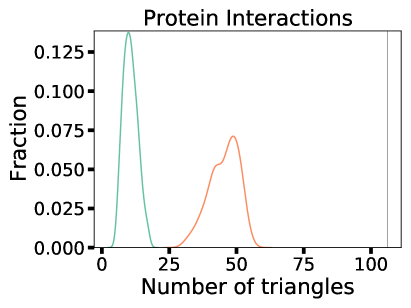
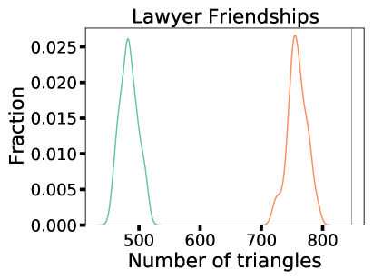
[Four histograms of triangle count]Four triangle count histograms, the k-core null model overlaps with the configuration model for Autonomous systems and Power Grid.

Figure 1. Distribution of the number of triangles from 50 random samples of graphs with a $k$-core sequence given by a real-world graph dataset and 50 random samples of graphs with a degree sequence given by a real-world graph dataset. The $k$-core samples have more triangles, and often the number of triangles in the dataset is within the range those observed in the random samples.

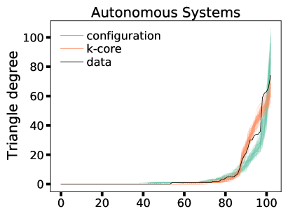
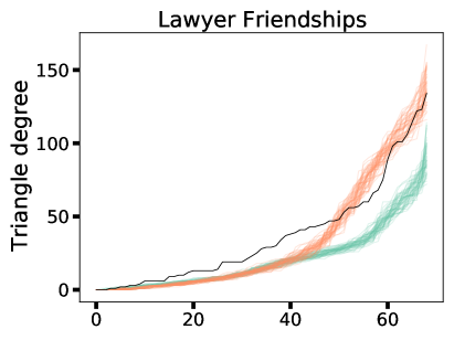
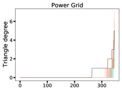
[Four exponential graphs]K-core triangle degree is consistently higher than the configuration model and closer to the true data.

Figure 2. Triangle degree sequences (given by the number of triangles adjacent to a given node) from 50 random samples of graphs with a $k$-core sequence given by a real-world graph dataset and 50 random samples of graphs with a degree sequence given by a real-world graph dataset. The $k$-core samples tend to match the triangle sequence more closely.

For our computational experiments here and in a number of the subsequent analyses, we use four graph datasets: an autonomous systems network (leskovec2005graphs, ), a protein structure network (milo2004superfamilies, ), a friendship network of lawyers working at the same firm (lazega2001collegial, ), and a power grid (son_kim_olave-rojas_alvarez-miranda_2018, ). For each dataset, we run our Markov-chain sampler for a number of steps equal to 100 times the number of edges in the graph, with input $k$-core sequence given by the dataset. We repeated this 50 times to get 50 random graphs with a prescribed $k$-core distribution.

We then compare the statistics of the resulting graph to the output of the configuration model. For this, we use 50 samples from a Markov-chain configuration model sampler for vertex-labeled simple graphs, using the double edge swap procedure described by Fosdick et al. (fosdick2018configuring, ).

As noted earlier in this section, one weakness of the configuration model is that it destroys local structure, and we observe this even on the small datasets considered here. Specifically, the total number of triangles in the configuration model samples is far below the number of triangles in the corresponding datasets (Figure 1).

The random samples from the prescribed $k$-core sequence have more triangles than those in the configuration model samples. Moreover, the distribution of the total number of triangles straddles the number of triangles in the autonomous systems dataset. Thus, the observed number of triangles in this datasets is unsurprising given the $k$-core sequence. In other words, we would not reject the null model of a random graph sampled uniformly at random from the space of graphs with the given $k$-core sequence, just based on the statistic of the number of triangles.

In addition to the total number of triangles, we also measure the triangle degree sequence in these random samples and compare them to the datasets (Figure 2). Here, the triangle degree of a node is the number of triangles in which it participates. We see that the triangle degree sequences given by the $k$-core sequence null model more closely match those of the data.

Taken together, the results of this subsection provide evidence that our $k$-core-based null model offers a substantially different baseline than the configuration model. In particular, for the datasets considered here, the core-based null model produces random samples with a larger number of triangles that capture some of the local structure in the graph. We will see in the next subsection that this same principle applies for motif analysis more generally.

Motif analysis

A longstanding application of null models for network analysis is the identification of important or unusual small subgraph patterns called network motifs (milo2002network, ). The main idea is to count the number of occurrences of several small subgraphs in a given dataset as well as in several random samples from a null model. “Motifs” are then subgraphs that appear significantly more or less often than in the null. Historically, the employed null model is the configuration model (milo2002network, ; milo2004superfamilies, ; fosdick2018configuring, ). Here, we consider both the configuration model and our $k$-core-based model as null models.

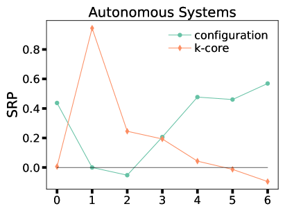
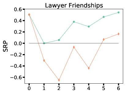
[Two line plots]K-core and configuration model diverge for all 7 subgraphs.

Figure 3. Subgraph ratio profile (SRP) plots under the $k$-core and configuration null models for four node subgraphs and triangles. The x-axis in the SRP plots are indexed by the seven subgraphs at the bottom.

In Figure 3 we consider the results of counting six different motifs consisting of six distinct (non-induced) subgraphs on four nodes each, as well as a motif consisting of the triangle so that we can view the results of the previous subsection in this context as well. To decide whether the number of copies of a given subgraph appears significantly more or less frequently than in a random baseline, a canonical approach is to the use the subgraph ratio profile (SRP), which essentially measures a normalized difference between the frequencies of the subgraph in the real network and in the random baseline. (We refer readers to Milo et al. (milo2004superfamilies, ) for the precise definition.) As a result, a positive SRP for a given subgraph indicates that the subgraph occurs more frequently in the real data than in a random baseline, while a negative SRP indicates that it occurs less frequently. Positive SRP values are thus taken as evidence that the corresponding subgraph is a meaningfully abundant motif in the network data.

Viewed in this context, we see that the SRP can be defined using any random-graph model that fixes some aspect of the structure of the real network. While the configuration model that fixes degrees is the standard approach, we can also define SRP values using the core-value model and ask whether we arrive at similar conclusions. As we see in Figure 3, the SRP values based on the core-value model are in fact quite different for two of our datasets, on autonomous systems and the social network on lawyers. In particular, we see that many SRP values are on opposite sides of $0$ across the two models, showing that a number of conclusions can change when we move a core-based null model. Moreover, these changes generally go in the conjectured direction based on the preservation of local structure: if we believe that the core-value model destroys less of the local structure in a network relative to the configuration model, then we would expect lower (and potentially negative) SRP values, and this is what see for many of the subgraphs in Figure 3. The results thus point to the crucial role in the choice of null model for interpreting these subgraph frequency questions — a type of issue that becomes feasible to ask given an efficient way to generate null graphs with fixed core-value sequences.

4.2. Edge-based statistics

To understand how the core-value model behaves in these types of applications, it is natural to explore some of its basic properties as well. Perhaps the most fundamental set of properties concern basic counts of edges and degrees.

When sampling based on a $k$-core description given by a dataset, a major difference with the configuration model is that the number of edges in the random sample can differ from those in the dataset. For a simple example, consider a 4-cycle and the graph obtained by adding one additional edge to the 4-cycle — all nodes in both graphs have a core value equal to two, but they differ in the number of edges. Here, we examine the distribution in the number of edges in random samples generated by our algorithm, where the core-value sequence is generated by a real-world dataset.

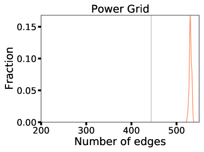
[Four histograms]K-core consistently has more edges than the real-world graph.

Figure 4. Distribution of the number of edges from 50 MCMC samples of graphs with a $k$-core sequence given by a real-world graph dataset. As expected, the number of edges in the random samples is different than in the original data, but the difference is not drastic.

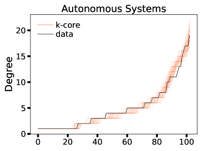
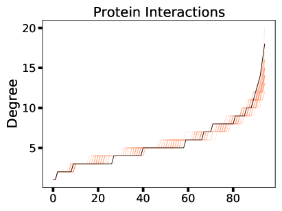
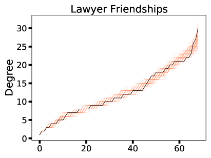
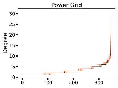
[Four line plots]For all four plots, frequency increases with degree.

Figure 5. Degree sequences from 50 MCMC samples of graphs with a $k$-core sequence given by a real-world graph dataset. The degree sequences of the random samples are similar (but not identical) to the degree sequences in the real-world data.

We use the same datasets and sampling procedure that we employed in the previous subsections. Figure 4 shows the number of edges in the resulting samples. We see that, for a given dataset, all of the random samples have a number of edges that is greater than or equal to the original data. Thus, the total number of edges in these datasets over the space of graphs with the same $k$-core sequence is concentrated above the observed number of edges. At the same time, though, the number of edges in the random sample is not drastically different.

We also compare the degree sequence of the random samples to those in the original data (Figure 5). The degree sequences largely resemble those in the original data, but are not exactly the same. Often, the samples from our algorithm produce graphs with a larger maximum degree than the empirical autonomous systems dataset.

4.3. Attribute-based assortativity

Table 1. Network assortativity $r$ with respect to several attributes in the Lawyers dataset. We list the z-score of the assortativity statistic with respect to 50 samples from the configuration and $k$-core-based model.

		z-score
Attribute	$r$	configuration	$k$-core
Status	0.55	21.29	3.92
Office Location	0.21	5.53	8.72.
Gender	0.12	2.50	0.31
Law School	0.05	1.80	0.79
Type of Practice	0.04	1.29	1.71

As a final investigation, we consider whether or not attribute-based assortativity is preserved under the configuration and core-value null models. The lawyers dataset has several attributes on each node, and we measure the network assortativity $r$ (newman2003mixing, ) for status at the firm (partner or associate), office location, gender, law school, and type of practice (litigation or corporate). Assortativity is positive for all of the attributes, i.e., there is a tendency for edges to appear between two nodes sharing the same attribute (Table 1).

As a baseline, we measure the assortativity levels under 50 samples of the configuration model and the core-value model and compute the same $z$-score as for the motif analysis. The assortativity scores are higher in the data than in both the null models (all of the $z$-scores in Table 1 are positive). For example, office location assortativity is overwhelmingly significant under either null. This is unsurprising, as neither null model is designed to capture mesoscale modular, community, or cluster structure within the network, and several of the attributes are known to correspond to meaningful cluster structure (peel2017ground, ).

At the same time, evaluating significance based on $z$-scores for some attributes could lead to different conclusions based on the choice of null model and the desired significance level. For example, the gender assortativity in the network is $0.12$, which is about 2.5 standard deviations above the mean with respect to the configuration model, but only 0.31 standard deviations above the mean with respect to the core-value model. Thus, gender assortativity may seem insignificant under the core-value null but significant under the configuration model null.

5. Conclusion

The $k$-core decomposition is a fundamental graph-theoretic concept that assigns each node $v$ a core-value equal to the largest $c$ such that $v$ belongs to a subgraph of $G$ of minimum degree $c$. Drawing on this concept, we have proposed a new family of random graphs that can serve as a class of null models in network analysis, obtained by randomly sampling from the set of all graphs with a given core-value sequence. Our sampling method exploits the rich combinatorial structure of the $k$-core decomposition; we construct a novel Markov chain on the set of all graphs of a given core-value sequence, show that the state space is connected with respect to this transition, and establish that the chain can be used to generate near-uniform samples from this set of graphs.

The approach opens up a number of intriguing further directions of potential theoretical and empirical interest. One question noted earlier is to try establishing bounds on the mixing rate of the Markov chain we have defined. Such questions are in general quite challenging, since the mixing even of simpler chains remains open; we note that many of these chains have proved valuable for sampling even in the absence of provable guarantees. A second question, related to our solution of the realizability question for core-value sequences, is to study extremal questions over the set of graphs realizing a given core-value sequence; for example, what is the minimum or maximum number of edges that a graph with a given core-value sequence can have? Finally, in a more empirical direction and motivated by our findings on network motifs, it will be interesting to characterize the kinds of network properties for which the configuration model and our core-value model produce systematically different results. Such comparisons can begin to provide insight into the broader consequences of our choice of null models in network analysis.

References

- [1] Yael Artzy-Randrup and Lewi Stone. Generating uniformly distributed random networks. Physical Review E, 72(5):056708, 2005.
- [2] Edward A Bender and E Rodney Canfield. The asymptotic number of labeled graphs with given degree sequences. Journal of Combinatorial Theory, Series A, 24(3):296–307, 1978.
- [3] Béla Bollobás. A probabilistic proof of an asymptotic formula for the number of labelled regular graphs. European Journal of Combinatorics, 1(4):311–316, 1980.
- [4] Shai Carmi, Shlomo Havlin, Scott Kirkpatrick, Yuval Shavitt, and Eran Shir. A model of internet topology using k-shell decomposition. Proceedings of the National Academy of Sciences, 104(27):11150–11154, 2007.
- [5] Philip S Chodrow. Configuration models of random hypergraphs. Journal of Complex Networks, 8(3):cnaa018, 2020.
- [6] Sheshayya A Choudum. A simple proof of the Erdos-Gallai theorem on graph sequences. Bulletin of the Australian Mathematical Society, 33(1):67–70, 1986.
- [7] Fan Chung and Linyuan Lu. The average distances in random graphs with given expected degrees. Proceedings of the National Academy of Sciences, 99(25):15879–15882, 2002.
- [8] Fan Chung and Linyuan Lu. Connected components in random graphs with given expected degree sequences. Annals of combinatorics, 6(2):125–145, 2002.
- [9] Fan Chung, Linyuan Lu, and Van Vu. The spectra of random graphs with given expected degrees. Internet Mathematics, 1(3):257–275, 2004.
- [10] Pol Colomer-de Simón, M Angeles Serrano, Mariano G Beiró, J Ignacio Alvarez-Hamelin, and Marián Boguná. Deciphering the global organization of clustering in real complex networks. Scientific reports, 3:2517, 2013.
- [11] Sergey N Dorogovtsev, Alexander V Goltsev, and Jose Ferreira F Mendes. K-core organization of complex networks. Physical review letters, 96(4):040601, 2006.
- [12] Mikhail Drobyshevskiy and Denis Turdakov. Random graph modeling: A survey of the concepts. ACM Computing Surveys (CSUR), 52(6):1–36, 2019.
- [13] Paul Erdös and Tibor Gallai. Graphs with given degrees of vertices, math. Mat. Lapok, 11:264–274, 1960.
- [14] Bailey K Fosdick, Daniel B Larremore, Joel Nishimura, and Johan Ugander. Configuring random graph models with fixed degree sequences. SIAM Review, 60(2):315–355, 2018.
- [15] Minas Gjoka, Maciej Kurant, and Athina Markopoulou. 2.5 k-graphs: from sampling to generation. In 2013 Proceedings IEEE INFOCOM, pages 1968–1976. IEEE, 2013.
- [16] S Louis Hakimi. On realizability of a set of integers as degrees of the vertices of a linear graph. i. Journal of the Society for Industrial and Applied Mathematics, 10(3):496–506, 1962.
- [17] Václav Havel. A remark on the existence of finite graphs. Casopis Pest. Mat., 80:477–480, 1955.
- [18] Lauri Kovanen, Márton Karsai, Kimmo Kaski, János Kertész, and Jari Saramäki. Temporal motifs in time-dependent networks. Journal of Statistical Mechanics: Theory and Experiment, 2011(11):P11005, 2011.
- [19] Ricky Laishram, Ahmet Erdem Sariyüce, Tina Eliassi-Rad, Ali Pinar, and Sucheta Soundarajan. Measuring and improving the core resilience of networks. In Proceedings of the 2018 World Wide Web Conference, pages 609–618, 2018.
- [20] Emmanuel Lazega. The collegial phenomenon: The social mechanisms of cooperation among peers in a corporate law partnership. Oxford University Press on Demand, 2001.
- [21] Jure Leskovec, Jon Kleinberg, and Christos Faloutsos. Graphs over time: densification laws, shrinking diameters and possible explanations. In Proceedings of the eleventh ACM SIGKDD international conference on Knowledge discovery in data mining, pages 177–187, 2005.
- [22] Priya Mahadevan, Dmitri Krioukov, Kevin Fall, and Amin Vahdat. Systematic topology analysis and generation using degree correlations. ACM SIGCOMM Computer Communication Review, 36(4):135–146, 2006.
- [23] Fragkiskos D Malliaros, Christos Giatsidis, Apostolos N Papadopoulos, and Michalis Vazirgiannis. The core decomposition of networks: Theory, algorithms and applications. The VLDB Journal, 29(1):61–92, 2020.
- [24] Ron Milo, Shalev Itzkovitz, Nadav Kashtan, Reuven Levitt, Shai Shen-Orr, Inbal Ayzenshtat, Michal Sheffer, and Uri Alon. Superfamilies of evolved and designed networks. Science, 303(5663):1538–1542, 2004.
- [25] Ron Milo, Nadav Kashtan, Shalev Itzkovitz, Mark EJ Newman, and Uri Alon. On the uniform generation of random graphs with prescribed degree sequences. arXiv preprint cond-mat/0312028, 2003.
- [26] Ron Milo, Shai Shen-Orr, Shalev Itzkovitz, Nadav Kashtan, Dmitri Chklovskii, and Uri Alon. Network motifs: simple building blocks of complex networks. Science, 298(5594):824–827, 2002.
- [27] Michael Molloy and Bruce Reed. A critical point for random graphs with a given degree sequence. Random structures & algorithms, 6(2-3):161–180, 1995.
- [28] Michael Molloy and Bruce Reed. The size of the giant component of a random graph with a given degree sequence. Combinatorics probability and computing, 7(3):295–305, 1998.
- [29] Mark EJ Newman. Mixing patterns in networks. Physical review E, 67(2):026126, 2003.
- [30] Mark EJ Newman, Steven H Strogatz, and Duncan J Watts. Random graphs with arbitrary degree distributions and their applications. Physical review E, 64(2):026118, 2001.
- [31] Chiara Orsini, Marija M Dankulov, Pol Colomer-de Simón, Almerima Jamakovic, Priya Mahadevan, Amin Vahdat, Kevin E Bassler, Zoltán Toroczkai, Marián Boguná, Guido Caldarelli, et al. Quantifying randomness in real networks. Nature communications, 6(1):1–10, 2015.
- [32] Leto Peel, Daniel B Larremore, and Aaron Clauset. The ground truth about metadata and community detection in networks. Science advances, 3(5):e1602548, 2017.
- [33] Alessandra Sala, Lili Cao, Christo Wilson, Robert Zablit, Haitao Zheng, and Zhao Ben Y. Measurement-calibrated graph models for social network experiments. In Proceedings of the 19th international conference on World wide web, pages 861–870, 2010.
- [34] Shai S Shen-Orr, Ron Milo, Shmoolik Mangan, and Uri Alon. Network motifs in the transcriptional regulation network of escherichia coli. Nature genetics, 31(1):64–68, 2002.
- [35] Kijung Shin, Tina Eliassi-Rad, and Christos Faloutsos. Corescope: Graph mining using k-core analysis—patterns, anomalies and algorithms. In 2016 IEEE 16th International Conference on Data Mining (ICDM), pages 469–478. IEEE, 2016.
- [36] Seung-Woo Son, Heetae Kim, David Olave-Rojas, and Eduardo Álvarez Miranda. Node information of chilean power grid with tap, Oct 2018.
- [37] Olaf Sporns and Rolf Kötter. Motifs in brain networks. PLoS Biol, 2(11):e369, 2004.
- [38] Isabelle Stanton and Ali Pinar. Constructing and sampling graphs with a prescribed joint degree distribution. Journal of Experimental Algorithmics (JEA), 17:3–1, 2012.
- [39] David Bruce Wilson. Generating random spanning trees more quickly than the cover time. In Gary L. Miller, editor, Proceedings of the Twenty-Eighth Annual ACM Symposium on the Theory of Computing, Philadelphia, Pennsylvania, USA, May 22-24, 1996, pages 296–303. ACM, 1996.
- [40] Jean-Gabriel Young, Giovanni Petri, Francesco Vaccarino, and Alice Patania. Construction of and efficient sampling from the simplicial configuration model. Physical Review E, 96(3):032312, 2017.