Dynamics and decay rates of a time-dependent two-saddle system

Abstract

The framework of transition state theory (TST) provides a powerful way for analyzing the dynamics of physical and chemical reactions. While TST has already been successfully used to obtain reaction rates for systems with a single time-dependent saddle point, multiple driven saddles have proven challenging because of their fractal-like phase space structure. This paper presents the construction of an approximately recrossing-free dividing surface based on the normally hyperbolic invariant manifold in a time-dependent two-saddle model system. Based on this, multiple methods for obtaining instantaneous (time-resolved) decay rates of the underlying activated complex are presented and their results discussed.

I Introduction

One of the central aims in the field of chemical reaction dynamics is the accurate determination of reaction rates. This is not just an abstract problem of academic (or basic) concern Truhlar et al. (1983); Marcus (1992); Truhlar et al. (1996); Komatsuzaki and Berry (2001), but also a practical problem with many potential applications in complex reactions Anslyn and Dougherty (2006); Harper et al. (2011); Chill et al. (2014); Kramer et al. (2015); Chen et al. (2017). The possibility of optimizing reaction rates by external driving could perhaps take these applications further in offering improvements to throughput and efficiency.

Multi-barrier reactions were considered early Miller (1968, 1979) in the context of quantum mechanical tunneling through barriers at constant energy. In this M-problem, the periodic orbit between the barriers gives rise to the possibility of an infinite number of returns to the turning point from which tunneling can proceed. The return times are usually not commensurate with the period, either because of coupling to other degrees of freedom—such as from the bath—or because of variations in the potential. In such cases, the coherence in the returns is altered, changing the nature of the dynamics in ways that we address in this work.

Problems involving fluctuating Doering and Gadoua (1992); Maddox (1992) or oscillating Lehmann et al. (2000a, b, 2003) barriers have also received significant attention leading to, for example, the identification of the phenomenon of resonant activation Van den Broeck (1993); Hänggi (1994). While the approaches originally focused on the overdamped regime Doering and Gadoua (1992); Lehmann et al. (2000a), underdamped systems were later examined Shepherd and Hernandez (2001); Lehmann et al. (2003). For example, mean first passage times have been employed to calculate (diffusion) rates in spatially periodic multi-barrier potentials. Therein, various static Shepherd and Hernandez (2002a) as well as stochastically driven Shepherd and Hernandez (2002b); Moix et al. (2004) cases have been characterized primarily through numerical methods.

In the current context, the main challenge in a multi-saddle system comes from the unpredictability of states in the intermediate basin. A reactant entering this region may leave either as a reactant or product depending on the exact initial conditions Vogelaere and Boudart (1955); Miller (1976); Pollak et al. (1980); Carpenter (2005). Historically, this challenge has been approached by categorizing reactions into two classes Miller (1976); Pechukas (1976, 1981): Direct reactions exhibit a single transition state (TS). Complex reactions, on the other hand, have two clearly separated TSs. The potential well between those barriers is assumed to be sufficiently deep that it gives rise to a long-lived collision complex. Trajectories passing through one TS enter this collision complex and hence cannot be correlated to trajectories passing through the other TS. In reality, however, a reaction cannot always be uniquely classified. These concerns were addressed in a unified theory by Miller Miller (1976), and later refined by Pollak and Pechukas Pollak and Pechukas (1979) so as to address shallow potential wells. While an important advancement, this theory still treats the saddle’s interactions statistically, thereby neglecting dynamical effects like resonances. Moreover, they considered multi-step reactions in which the positions and heights of the barriers are time-independent. Last, there are numerous publications on valley-ridge inflection points, which are typically described by a normal TS followed by a shared one Carpenter (2005); Rehbein and Carpenter (2011); Collins et al. (2013).

Craven and Hernandez Craven and Hernandez (2016) recently examined a four-saddle model of ketene isomerization influenced by a time-dependent external field. They encountered complicated phase space structures similar to those in systems with closed reactant or product basins Junginger et al. (2017). As a result, their analysis was limited to local dividing surfaces and no reaction rates were calculated. Moreover, successfully calculating instantaneous rates based on a globally recrossing-free DS attached to the normally hyperbolic invariant manifold (NHIM) of a time-dependent multi-saddle system has—to our knowledge—not yet been reported.

In this paper, we address the challenge of determining the instantaneous TS decay rate for systems that not only feature multiple barriers along the reaction path, but that are also time-dependent. Specifically, we investigate an open, time-dependent two-saddle model with one degree of freedom (DoF) as introduced in Sec. II.1. The theoretical framework along with the numerical methods used throughout the paper are described in Secs. II.2 through II.4. We then discuss the system’s phase space structure under the influence of periodic driving at different frequencies in Sec. III. By leveraging unstable trajectories bound between the saddles, we can construct an almost globally recrossing-free DS associated with the so-called geometric cross in Sec. IV. The DS is used in Sec. V to calculate instantaneous decay rates and averaged rate constants for the underlying activated complex using different methods. Thus we report a detailed analysis of the nontrivial phase space structure of the chemical M-problem and the calculation of its associated decay rates.

II Methods and materials

II.1 Time-dependent two-saddle model system

In this paper, we investigate the properties of multi-barrier systems by considering a 1-DoF model potential featuring two Gaussian barriers whose saddle points are centered at $x=$\pm 1$$. Initially, both barriers are placed at the same level. As we are interested in considering the time-dependent case, however, we drive the barrier’s heights $B_{\varphi}(t)$ sinusoidally in opposite phases. That is, we use the same amplitude and frequency $\omega$ for both saddles, but opposite initial phases $\varphi\in\quantity{0,\pi}$. This leads to the potential

$$V(x,t) =B_{0}(t)\mathrm{e}^{-(x+1)^{2}}+B_{\pi}(t)\mathrm{e}^{-(x-1)^{2}}$$ (1a)

$$\mbox{with\quad}B_{\varphi}(t) =\frac{7}{4}+\frac{1}{4}\sin(\omega t+\varphi)\,\text{.}$$ (1b)

The oscillation frequency $\omega$ is a free parameter that can be varied relative to the other natural time scales of the system at a given fixed total energy. At an arbitrary time, one of the barriers will be larger than the other. For example, when the second barrier is larger, the potential takes a shape such as that shown at the top of Fig. 1(b). Throughout this paper, dimensionless units are used to explore the range of phenomena that can arise from varying the relative timescales of the system and the driving.

II.2 Dividing surfaces and the NHIM

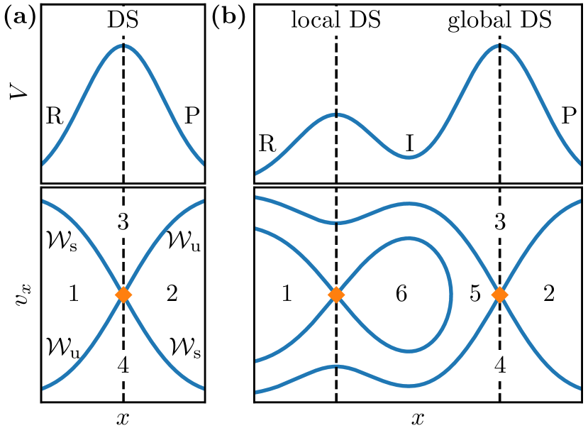
Figure 1: Typical structures of static potentials $V(x)$ and their corresponding phase spaces $x$–$v_{x}$ with one and two barriers in panels (a) and (b), respectively. The potential barriers separate reactant (R) and product (P) states. The two-barrier case features an additional intermediate (I) state in between. The maxima are associated with a hyperbolic fixed point (diamonds) and a dividing surface (indicated by dashed vertical lines) each. The corresponding manifolds divide the phase space into four distinct, numbered regions in panel (a) and six regions in panel (b). See Secs. II and III.1 for details.

Reactants and products on the canonical potential energy surface (PES) are usually separated by a DS often associated with a rank-1 saddle, such as that shown in Fig. 1(a), whose unstable direction identifies the reaction coordinate. The maximum energy configuration along the corresponding one-dimensional minimum energy path Glasstone et al. (1941); Fukui (1970); Kato and Fukui (1976) $x$ is called the TS Eyring (1935); Wigner (1937); Pechukas (1981); Truhlar et al. (1996). In transition state theory (TST), the local decay rate is obtained from the flux through the DS.

A DS is locally recrossing-free if no particle pierces it more than once before leaving some pre-determined interaction region around the saddle. In this case, the decay rates (to exit the interaction region) as determined by the DS are locally exact. We refer to a DS as being globally exact or recrossing-free if the above is true independent of the choice of the interaction region as long as said regions do not overlap with the stable reactant or product regions Feldmaier et al. (2019a). Using this definition avoids inherent recrossings caused by reflections in closed reactant or product basins Junginger et al. (2017). In this paper, we only address transitions over barriers in series, and we do not address the parallel case in which a reaction could access more than one distant barrier. The scope of the definitions of globally exact and recrossing-free is therefore limited accordingly.

Every saddle point of a $d$-DoF potential is associated with $(2d-1)$-dimensional stable and unstable manifolds $\mathcal{W}_{\mathrm{s}}$ and $\mathcal{W}_{\mathrm{u}}$ in phase space—cf. Fig. 1(a). Their $(2d-2)$-dimensional intersection is called the NHIM Lichtenberg and Liebermann (1982); Hernandez and Miller (1993); Hernandez (1993); Ott (2002); Wiggins (2013) and describes the unstable subspace of particles trapped on the saddle. It is noted with a diamond in Fig. 1(a). Depending on the convention used, the time-evolution of the NHIM or of a single point on the NHIM forms the TS trajectory Feldmaier et al. (2019a). A ($2d-1$)-dimensional DS can be constructed by attaching it to the NHIM, which works even for time-dependent driving. This particular DS is locally recrossing-free as long as particles do not cross far away from the NHIM Komatsuzaki and Berry (1999); Li et al. (2006a, b, 2009). However, it does not have to be globally recrossing-free if, e. g., the system features multiple barriers or valleys with sharp turns.

In TST, one typically uses the saddle point as the TS itself, but the variational principle clearly suggests that the DS can be moved away from it. In practice, this has led to applications in which the DS is associated with the saddle point. However, not only is this strong association not necessary, it is even possible that the NHIM (which anchors the DS) can be disconnected. Indeed, we find in the current problem that the optimal NHIM consists of multiple, disjoint sets. As seen in Sec. III, such structure can emerge from the interaction of multiple saddles. Those parts of the NHIM not associated with a saddle can nevertheless be used to construct a DS as before, and may feature fewer global recrossings compared to a DS associated uniquely with a single saddle point. The question of whether such a DS with fewer or even no recrossings can be found in a driven multi-saddle system has led to the central results of this work.

II.3 Revealing geometric structures

The geometric structure of the phase space can be revealed using the Lagrangian descriptor (LD) Mendoza and Mancho (2010); Mancho et al. (2013); Craven and Hernandez (2015); Junginger and Hernandez (2016); Craven and Hernandez (2016) defined by

$$\mathcal{L}(x_{0},v_{0},t_{0})=\int_{t_{0}-\tau}^{t_{0}+\tau}\differential{t}\norm{v(t)}$$ (2)

for a given initial position $x_{0}$, velocity $v_{0}$, and time $t_{0}$. It measures the arc length of a trajectory $x(t)$ in the time interval $t_{0}-\tau\leq t\leq t_{0}+\tau$. A local minimum in the LD arises when the particle covers the minimum distance in the interval $t_{0}-\tau\leq t\leq t_{0}+\tau$. It consequently remains longer in the interaction region when integrating forwards or backwards in time, and thus provides a signature for the presence of a stable or unstable manifold, respectively.

The LD has the advantage that it is conceptually very simple and that it can be applied to practically any system. This makes it suitable for a first visual inspection. As discussed in Ref. Bardakcioglu et al. (2018), however, it features a nontrivial internal structure. Numerically determining the exact position of stable and unstable manifolds is therefore difficult.

A numerically simpler scheme is based on the concept of reactive (and nonreactive) regions as described in Refs. Bardakcioglu et al. (2018); Feldmaier et al. (2019a). It discriminates initial conditions by first defining an interaction region in position space that encompasses the relevant dynamics. Particles are then propagated forwards and backwards in time until they leave said interaction region. In both directions of time, a particle can end up as either reactant (R) or product (P). This leads to four possible classifications for a given initial condition as shown in Fig. 1(a) for each of the four regions: 1. nonreactive reactants $\mathrm{R}\to\mathrm{R}$, 2. nonreactive products $\mathrm{P}\to\mathrm{P}$, 3. reactive reactants $\mathrm{R}\to\mathrm{P}$, and 4. reactive products $\mathrm{P}\to\mathrm{R}$. Similar concepts have been introduced in, e. g., Ref. Craven and Hernandez (2016).

Such a classification for the initial conditions has to be extended to include the consequences of a local minimum between the saddles of the reacting system of Eq. (1). A low-energy particle trapped near this local minimum [cf. Fig. 1(b)] would lead to diverging computation times because it may never leave the interaction region. To solve this problem, an additional termination condition is introduced, whereby any particle that crosses the potential minimum a specified number of times $n_{\mathrm{mc}}$ is classified as an intermediate (I) particle. Consequently, up to nine different regions in phase space can be distinguished for any given value of $n_{\mathrm{mc}}$.

Using the concept of reactive regions, stable and unstable manifolds can be revealed as borders between adjacent regions. Their closure’s intersections form the NHIM. The algorithm used to calculate points of the NHIM is based on the binary contraction method (BCM) introduced in Ref. Bardakcioglu et al. (2018). It starts by defining a quadrangle with one corner in each of the phase space regions surrounding the manifold intersection. The quadrangle is then contracted by successively determining the region corresponding to an edge’s midpoint and moving the appropriate adjacent corner there. The BCM is therefore effectively composed of four intertwined classical bisection algorithms. To reliably identify the initial corners, we modify the BCM slightly as detailed in Appendix A.

II.4 Calculating decay rates

The existence of a NHIM of codimension 2 and its role in determining the chemical reaction rate brings an additional concern. Namely, what is the degree of instability of the TS as determined by the decay of trajectories that start in the proximity of the NHIM? In a time-dependent—e. g. driven—environment, this instantaneous decay will be time-dependent as well. Nevertheless, it can be assigned a single characteristic decay rate constant when the time-dependence is periodic by taking the average over the period Lehmann et al. (2000a); Feldmaier et al. (2019b).

In this paper, we implement three different methods, summarized in Appendix B, for calculating decay rates: (i) The ensemble method Lehmann et al. (2000a); Feldmaier et al. (2019b) yields instantaneous (time-resolved) rates by propagating a large number of particles. It is computationally expensive but conceptually simple. (ii) The local manifold analysis (LMA) Feldmaier et al. (2019b, 2020) accelerates the computation of instantaneous rates by leveraging the linearized dynamics near the NHIM. (iii) If only average rate constants are desired, the Floquet rate method Craven et al. (2014); Feldmaier et al. (2019b) can be used instead while requiring even less computational resources.

In the cases resolving the dynamics of the two-barrier problem of Eq. (1), all three generally converge within reasonable time. However, they each involve different assumptions which might have led to different results, and which can provide complementary interpretations about the underlying dynamics. As shown in the results sections, all three lead to decay rates in excellent agreement. The repetition thus also serves to provide assurance in the reported values.

III Geometric structure of the two-saddle system

The phase space structure of the model system introduced in Sec. II.1 is highly dependent on the driving frequency $\omega$. In the following we will give a qualitative overview of the behavior the system can exhibit.

III.1 Limiting cases

A static two-saddle system akin to Eq. (1) with $\omega=0$ exhibits the phase space structure shown in Fig. 1(b). The saddle tops are associated with hyperbolic fixed points whose stable and unstable manifolds each form a cross. If the first saddle is smaller than the second one, two of its manifolds constitute a homoclinic orbit. In this case, the phase space is composed of six regions, namely 1. nonreactive reactants $\mathrm{R}\to\mathrm{R}$, 2. nonreactive products $\mathrm{P}\to\mathrm{P}$, 3. reactive reactants $\mathrm{R}\to\mathrm{P}$, 4. reactive products $\mathrm{P}\to\mathrm{R}$, 5. particles that react over the first saddle but get reflected at the second $\mathrm{R}\to\mathrm{I}\to\mathrm{R}$, and 6. intermediate particles that are trapped between the saddles $\mathrm{I}\to\mathrm{I}$.

Likewise, if the driving frequency is sufficiently large ($\omega\to\infty$), the particle will effectively see an average static potential in which it must cross two similar static barriers of equal height. As the energy is conserved, once the particle crosses the first barrier, it necessarily crosses the second barrier. This results in a phase space structure similar to that for the static case of Fig. 1(b)—although with heteroclinic orbits connecting the hyperbolic fixed points.

In such (effectively) static cases, it is straightforward to define a global recrossing-free DS. In a 1-DoF constant energy system, if (and only if) a particle crosses the highest saddle, it has demonstrated to have enough energy to react over all saddles. Since the largest barrier therefore unambiguously determines whether a particle reacts or not, its associated local DS becomes the global (recrossing-free) DS.

While this holds true for static systems, dynamically driven systems may exhibit much richer dynamics. For example, in the case of an alternating pair of dominant barriers, as in the model of Eq. (1), the naive DS jumps discontinuously from one side to the other twice per period. As a result there exist reactive trajectories that never cross the DS. Instead, the latter jumps over the former leading to an inconsistent description of the reaction. Addressing this issue by defining particles between the local DSs as reacting the moment the dominant saddle changes would lead to more problems, e. g., unphysical Dirac delta peaks in the reaction rate. To solve this issue, the system has to be treated as a whole.

III.2 Intermediate driving frequency

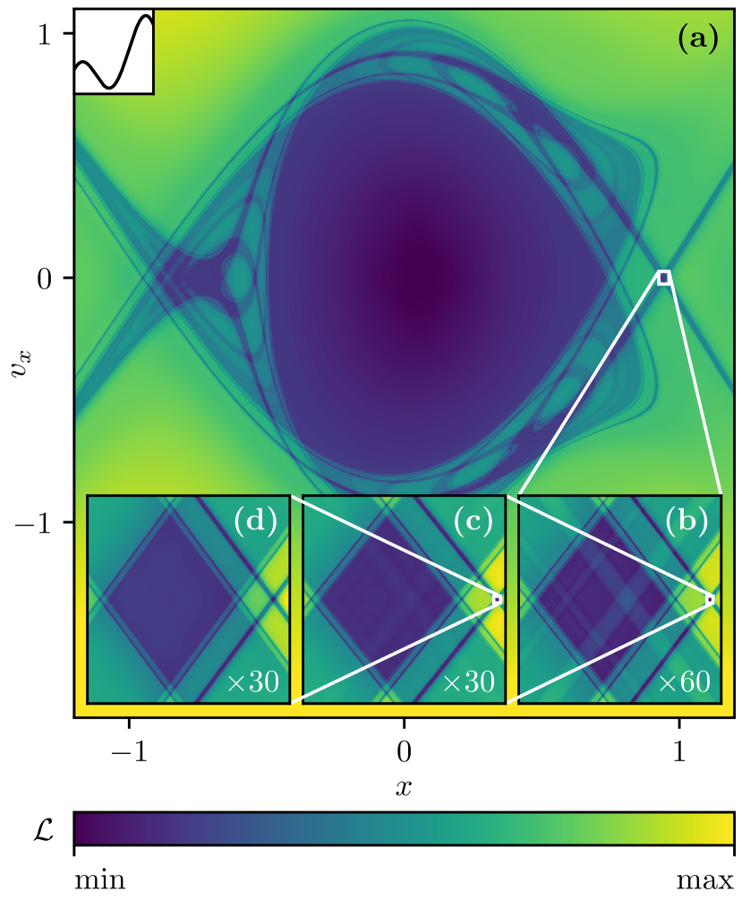
Figure 2: Phase space structure for the time-dependent potential in Eq. (1) with $\omega=\pi$ at $t_{0}=3/2$ as revealed by the Lagrangian descriptor $\mathcal{L}$ given in Eq. (2) with $\tau=16$. Although the two geometric crosses seen in Fig. 1(b) are still present in panel (a), they now exhibit a complicated substructure involving a vast number of homoclinic and heteroclinic points as well as homoclinic and heteroclinic orbits. The progressively zoomed cutouts shown in subpanels (b) through (d) exhibit self-recurring structures. Labels in the bottom right corners indicate the corresponding enlargement from the previous zoom level. The potential at time $t_{0}$ is indicated in the top left inset of panel (a).

The limiting cases discussed so far result in effectively static systems. Since we are interested in novel and nontrivial behavior, however, we will now turn to intermediate driving frequencies. These can exhibit varying degrees of complexity as a function of the driving frequency $\omega$. An example of such non-trivial behavior with a highly complex phase space is shown in Fig. 2. We use the LD defined in Sec. II.3 for visualization since it is very general and requires little knowledge about the system.

The geometric structure was obtained for the driven potential $V(x,t)$ of Eq. (1) at an intermediate driving frequency $\omega=\pi$. The general shape of the boundaries separating reactive and nonreactive regions (cf. Fig. 1(b)) is still vaguely visible. However, the precise position of the crossing points between the stable and unstable manifolds can no longer be determined. This family of crossing points together with the associated stable and unstable manifolds within their vicinity appears as a cross that has arisen from all of these geometric considerations. For simplicity, we define it as a geometric cross throughout this work. Note that this term is not meant to be a precise mathematical structure but rather an illustrative concept for describing the complex phase space of the system under study.

The fractal-like geometric crosses seen in the series of Figs. 2(a)–(d) for a finite $\tau$ suggests a fractal structure at all scales for $\tau\to\infty$. This structure emerges from particles trapped between the two saddles. For example, a reactant can enter the intermediate region over the left saddle, be reflected multiple times at both saddles, and finally leave the interaction region over the right saddle as a product. The number of reflections is in this case highly dependent on the particular initial conditions as a result of the system being chaotic. In turn, this leads to a discontinuity in the LD, and eventually to the self-recurring patterns of a fractal structure.

Figure 2 also supports the observation of geometric structures at a given time that are thinner near the dominant saddle compared to the lower energy saddle. In Fig. 2(a), when the right barrier is dominant, particles initialized near the higher saddle start with higher potential energy and therefore have a lower chance of being reflected. As a result, fewer of these particles linger in the interaction region and the phase space structures are thinner. While this may be an interesting observation, the geometric cross near the dominant barrier is still highly fractal. There are no isolated, weakly fractal geometric crosses that could reasonably be tracked numerically. Consequently, we cannot make meaningful statements about a globally recrossing-free DS.

III.3 Slow driving frequency

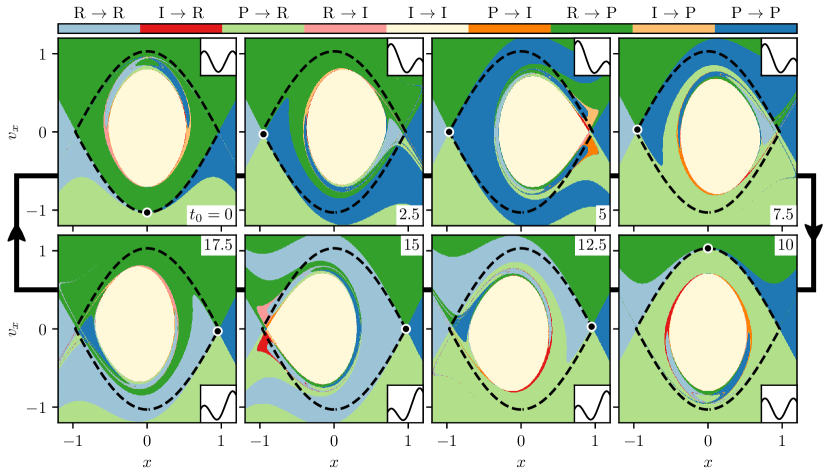
Figure 3: Reactive regions for potential (1) with $\omega=\pi/10$ and $n_{\mathrm{mc}}=8$ as a function of time $t_{0}$ (cf. inset labels). The color (or shaded) legend at the top indicates whether a particle starts or ends in the reactant (R), intermediate (I), or product (P) state. The position of the point on the NHIM associated with the primary geometric cross (black dot) is tracked across a full period (TS trajectory, black dashed line). The insets in the upper right corner of the top row panels and the lower right corner of the bottom row panels illustrate the potential at the corresponding initial time $t_{0}$.

The previous sections have shown the range of complexity the model system (1) can exhibit. We now need to move from the aesthetically pleasing structures of Fig. 2 to a more rigorous identification of the globally recrossing-free DS. To do so, we switch to a lower driving frequency $\omega=\pi/10$ which is simpler to analyze but still exhibits nontrivial behavior. Additionally, we employ the concept of reactive regions as described in Sec. II.3 instead of the LD. The partitioning of the phase space into nine distinct regions allows to make quantitative assessments more easily.

Application of this analysis to $V(x,t)$ with $\omega=\pi/10$ leads to the time-dependent regions shown in Fig. 3. Although fractal-like structures still remain, they are less pronounced and mostly concentrated around whichever saddle happens to be the lower saddle at a given instance. The higher saddle, on the other hand, is accompanied by a clearly visible geometric cross, where the four regions known from the one-saddle case (no intermediate states) meet. The regions are also arranged in the same way: $\mathrm{R}\to\mathrm{P}$ on top, $\mathrm{R}\to\mathrm{R}$ to the left, $\mathrm{P}\to\mathrm{P}$ to the right, and $\mathrm{P}\to\mathrm{R}$ below. In the following, we refer to this geometric cross as the primary geometric cross.

IV The geometric cross

We will now analyze the primary geometric cross and its associated TS trajectory in more detail. Its time-dependent position can be tracked precisely over a full period using the algorithm described in Sec. II.3 and Appendix A. The result is marked as a series of black dots in Fig. 3. The corresponding trajectory connecting those dots is indicated as a black dashed line.

IV.1 Global transition state trajectory

The primary geometric cross associated with the instantaneously higher saddle in Fig. 3 remains on the barrier nearly as long as the barrier remains dominant. However, when the barriers’ heights approach each other, the geometric cross quickly moves from one barrier to the other in the following way. The geometric cross begins to rapidly accelerate towards the middle ($x=0$). It crosses the local potential minimum exactly when both saddle points are level (e. g. $t_{0}=10$) and continues in the same direction until it is located near the now higher saddle (e. g. $t_{0}=15$). The reverse happens in the following half period, thereby forming a closed trajectory with the same period $T_{1}=20$ as the potential $V(x,t)$ (dashed line in Fig. 3).

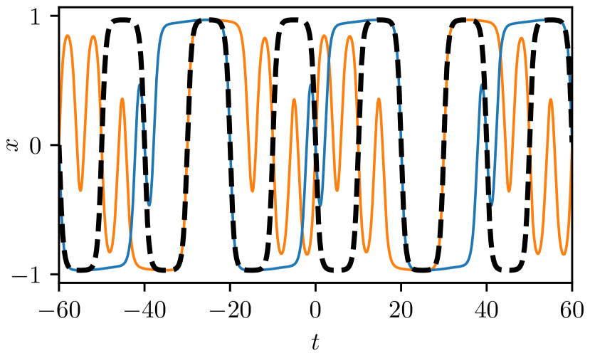
Figure 4: Examples of typical periodic trajectories $x(t)$ with periods $T_{2}=40$ (darker gray or blue) and $T_{3}=60$ (lighter gray or orange) for potential (1) with $\omega=\pi/10$. The primary TS trajectory from Fig. 3 with period $T_{1}=20$ (black dashed line) is shown for comparison.

This primary geometric cross marks the position of a particle on an unstable periodic trajectory trapped in the interaction region. The particle on this trajectory oscillates between the saddles with a period of $T_{1}=20$ so that it is always located near the higher saddle. Many other unstable periodic trajectories associated with geometric crosses—i. e. hyperbolic fixed points—in phase space have also been found for particles in the interaction region. Two such trajectories are shown in Fig. 4. They are typical of an increased degree of structure relative to the primary TS trajectory. All such trajectories together form the system’s disjoint, fractal-like time-dependent NHIM. In contrast to the primary TS trajectory, however, all other trajectories have periods larger than $T_{1}$. The only exceptions to this observation are the local TS trajectories in the vicinities of the saddle maxima, which are also part of the global NHIM. These trajectories have the same period $T_{1}$ as the potential by construction.

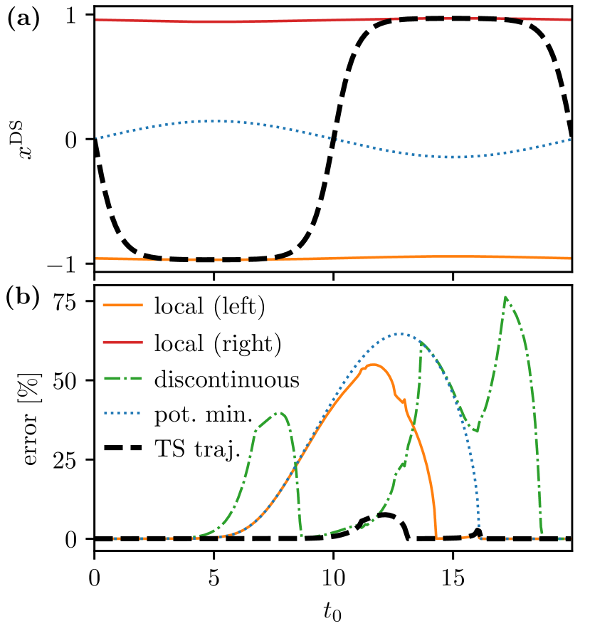
Figure 5: (a) Position $x^{\mathrm{DS}}$ and (b) percentage of trajectories with recrossings or classification errors as a function of time $t_{0}$ for various choices of their assignment as reactive or nonreactive. The assignment is performed according to the crossing of a specified DS associated with either the local (solid) or global (thick dashed) TS trajectories, the instantaneous potential minimum between the saddles (dotted), or the discontinuous TS trajectory jumping between the local ones (dash-dotted). For every $t_{0}$, an ensemble of ${10}^{6}$ particles with uniformly distributed velocities $$1.7$\leq v_{x}(t_{0})\leq$2.1$$ is initialized at $x(t_{0})=$-3$$ and propagated for $\Delta t=80$ time units. The attached DS is parallel to $v_{x}$ for all times. The right local DS is recrossing-free by construction since particles are started solely to the left of the saddles and is therefore not shown in (b). This specific choice for the ensemble is also the reason for the graph’s asymmetry.

The complex dynamics that arises from the moving barriers is also affected by the degree to which a given trajectory is decoupled from the barriers as it traverses the well between them. Although the energy of the minimum stays roughly constant, as indicated in Fig. 3, its position moves back and forth between the barriers as shown in Fig. 5(a) so that it is always closer to the lower barrier. This is a manifestation of the Hammond postulate Hammond (1955) but now applied to the negative potential. When the first (left) barrier dominates the dynamics, a locally nonrecrossing DS associated with it identifies the trajectories with sufficient energy to cross it, and those continue unabated across the well and the second barrier. As a consequence, a DS located at the well identifies the reactive trajectories equally well (or badly) in this regime. This is indicated in Fig. 5(b) by good identification when the activated particle continue past the second barrier or disagreement when misidentification of trajectories begin to be reflected across both. When the second (right) barrier dominates the dynamics, identifying reactive trajectories at a DS at the distant well allows the evolving trajectories to be reflected by the barrier leading to recrossings. Thus we find that the reaction dynamics in between the barriers—e. g. at the well—does not go through a single identifiable doorway. In turn, this points to the need for describing the dynamics—even in a local sense—through a geometric picture that spans the two barriers, e. g. the global NHIM.

Meanwhile, since the NHIM now consists of more than one trajectory, it is not necessarily obvious which of these is most suited for attaching a global DS. We can, however, set conditions the global TS trajectory should fulfill. First, for symmetry reasons, the trajectory should have the same period $T_{1}=20$ as the potential. Second, the global TS trajectory should approach the higher saddle’s local TS trajectory in the (quasi-)static limit $\omega\to 0$ (cf. Sec. III). The only trajectory found that matches both criteria is the primary TS trajectory introduced previously, see Fig. 5(a). The large featureless regions surrounding the trajectory in phase space additionally suggest that it affects a significant fraction of the system’s dynamics. We will therefore refer to this trajectory as the global TS trajectory.

IV.2 Comparison of dividing surfaces

The next task is to determine the degree to which the global TS trajectory gives rise to a recrossing-free DS. Numerically, this can be tested by attaching a DS to it as specified in the caption of Fig. 5, propagating an ensemble initialized near it, and recording the number and direction of DS crossings (or not) that transpire thereafter in the propagated trajectories. For simplicity, we consider only the most challenging cases in which the ensemble’s initial energies are chosen to be between the saddles’ minimum and maximum heights. The usual error in the DS is signaled by the existence of more than one crossing for the trajectories, and the fraction of such recrossings is used below as a measure for the DS’s quality.

For simplicity, we limit ourselves to DSs defined by $x=x^{\mathrm{DS}}(t)$, i. e., parallel to $v_{x}$. The results of this analysis are shown in Fig. 5(b). As can be seen, the global DS associated with the time-dependent geometric cross features error rates that are significantly reduced compared to the local DS fixed at the left barrier. One possible DS could be constructed by placing it at the instantaneous potential minimum—shown as the dotted curve in Fig. 5(a). It would be expected to be ineffective given that rates are usually determined by rate-limiting barriers, not valleys, in between reactants and products. Indeed, the recrossing errors found for this DS, shown in Fig. 5(b), were high and even worse than those from the use of the DS fixed at the left barrier. But the highest error rate comes from the naive attempt to treat the DS associated with the instantaneously higher saddle point as the global one. In this case, errors can arise from events beyond the recrossing of the DS. That is, there now exists the possibility that the discontinuous instantaneous DS can jump over the trajectory. It is the combination of recrossing and classification errors that leads to the jagged and large deviations in the $\mathrm{\char 37\relax}$ error seen for the naive discontinuous DS. As discussed in Appendix C, this can lead to misclassification of the reactivity of the trajectory.

Finally, we consider a local DS fixed at the right barrier. This choice would lead to no recrossing or classification errors for trajectories moving in the forward direction (from reactants to products). However, it would fail badly for trajectories moving in the backward direction by symmetry with our finding for the forward trajectories crossing the DS at the left barrier. Thus, the use of the global DS associated with the TS trajectory best captures the time-dependent geometry of the reaction.

Figure 6: Reactive regions analogous to Fig. 3 at $t_{0}=$0.25$$ with the addition of the DS (solid black line). (a) The simplest choice of a DS parallel to $v_{x}$ leads inevitably to recrossings as indicated. (b) The immediate region of the TS trajectory [shown as a dot in panel (a)], is enlarged, as indicated, to reveal the geometry of the ensemble (densely dotted) used in the rate calculations of Sec. V. The ensemble is sampled equidistantly on a line parallel to the unstable manifold $\mathcal{W}_{\mathrm{u}}$ at distance $x-x^{\mathrm{DS}}=$-1\text{\times}{10}^{-3}$$ from the TS trajectory at $x^{\mathrm{DS}}(t_{0})$. The manifolds $\mathcal{W}_{\mathrm{u}}$ and $\mathcal{W}_{\mathrm{s}}$ are given by the boundaries between reactive and nonreactive regions. The differential of $\mathcal{W}_{\mathrm{u}}$ is indicated by the sides $\Delta x$ and $\Delta v_{x}^{\mathrm{u}}$ of the slope.

Although this TS-trajectory DS is much better than any alternatives considered so far, it still exhibits an amount of recrossings that cannot be explained by numerical imprecision alone. Instead, recrossings are caused by the fractal-like phase space structure of the system: Figure 6(a), for example, shows the phase space structure at $t_{0}=$0.25$$. We can see a relatively large patch of nonreactive reactants (labeled $\mathrm{R}\to\mathrm{R}$, light blue) to the right of the DS. Particles in this patch leave the interaction region to the reactant (left) side forwards and backwards in time. Consequently, they need to cross the DS at least twice, which counts as a recrossing. An analogous argument can be applied to $\mathrm{P}\to\mathrm{P}$ regions to the left of the DS. The fractal-like phase space structure thus leads to numerous problematic patches of vastly different sizes, hence the two distinct peaks in Fig. 5(b).

A totally recrossing-free DS, by contrast, would necessarily have to divide the phase space such that $\mathrm{R}\to\mathrm{R}$ regions are always on the reactant side, and $\mathrm{P}\to\mathrm{P}$ regions always on the product side. This is not possible with a planar DS of any orientation due to the system’s fractal-like nature. A globally recrossing-free DS—if it exists—would have to curve as time passes because the entirety of the phase space between the saddle points has a clockwise rotating structure (including periodic trajectories on the NHIM, cf. Figs. 3 and 4). The periodicity of this system would then result in a fractal, spiral-like DS. Thus the next step in generalizing this theory would require the identification of a non-planar DS anchored at the TS trajectory which we leave as a challenge to future work.

V Reaction rate constants

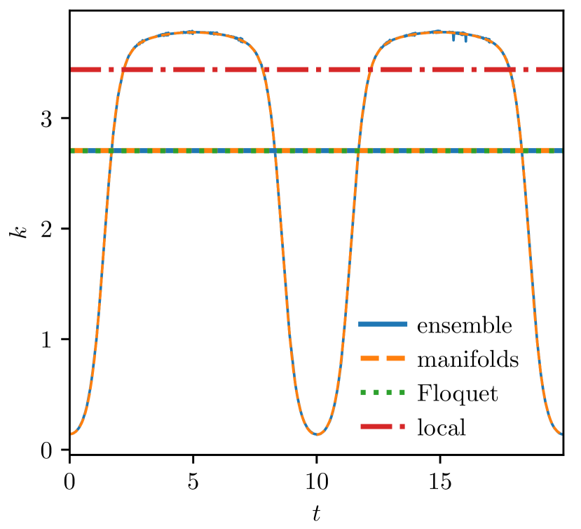
Figure 7: Various instantaneous reaction rates $k$ parameterized by time $t$ and associated with the global TS trajectory of the potential defined in Eq. (1) with $\omega=\pi/10$, and driving period $T_{1}=$20$$. The ensemble rate $k_{\mathrm{e}}(t)$ (blue solid) is obtained by propagation of 20 ensembles of ${10}^{5}$ particles each as described in Appendix B.1. The manifold rate $k_{\mathrm{m}}(t)$ (orange dashed) is obtained using Eq. (5). The Floquet rate constant $k_{\mathrm{F}}$ (green dotted) is obtained from Eq. (8). The mean rates, $\bar{k}_{\mathrm{e}}$ and $\bar{k}_{\mathrm{m}}$ (thick horizontal lines) are averaged over the period as defined in Eq. (3). For comparison, the Floquet rate constant $k_{\mathrm{F}}^{\mathrm{loc}}$ (red dash-dotted) of a single barrier’s local TS trajectory is also shown.

We can now calculate decay rate constants $k$ for the activated complex using the global TS-trajectory DS defined in Sec. IV. The patches leading to recrossing (cf. Sec. IV.2) are unproblematic in this case because the ensemble was selected close to the NHIM and thereby necessarily far from them, as can be seen in Fig. 6. The few recrossings that do still occur are artifacts from the numerical error in the propagation, and are sufficiently small in number that their effect is smaller than the numerical precision of the calculation.

In the following, we consider the three different possible approaches defined in Sec. II.4 in order to demonstrate their equivalence in multi-saddle systems. An example for the initial reactant ensemble and manifold geometry can be found in Fig. 6(b).

While the application of the LMA and the Floquet method to our model system are straightforward, applying the ensemble method poses a challenge: A finite ensemble of reactants—e. g. of size ${10}^{5}$ as implemented here—will mostly react within a short time—e. g. $2$ to $5$ units of time in the case shown here—compared to the period of driving $T_{1}=20$. Resolving the whole period with a single ensemble would therefore require an exponentially growing ensemble size. This would not be numerically feasible. Instead, multiple ensembles have been started at times $t_{j}$ incremented at equal intervals $\Delta t$, and set to $1$ in the current case. An instantaneous rate $k_{\mathrm{e}}(t;t_{j})$ can be obtained for each ensemble $j$. The instantaneous rate for the whole period $k_{\mathrm{e}}(t)$—independent of $t_{j}$—can then be recovered by concatenating the segments of each $k_{\mathrm{e}}(t;t_{j})$ for $t$ from $t_{j}$ to $t_{j+1}$. Compared to the first option, this approach scales linearly with the system’s period instead of exponentially leading to vastly decreased computing times and increased numerical stability.

The results are shown in Fig. 7. Since $k_{\mathrm{e}}(t)$ and $k_{\mathrm{m}}(t)$ are not constant in time, we additionally show the average

$$\bar{k}=\frac{1}{T_{1}}\int_{0}^{T_{1}}\differential{t}k(t)$$ (3)

over one period $T_{1}$ of the TS trajectory.

Figure 7 shows a large variation in the instantaneous reaction rate in the interval $$0.13$\lesssim k(t)\lesssim$3.85$$. Two features are distinctive. First, the rate $k(t)$ shows mostly flat plateaus during the time the TS trajectory is located near a saddle. This can be explained using Fig. 3: Although the phase space structure as a whole is undergoing significant changes during, e. g., $$2.5$\leq t\leq$7.5$$, the local vicinity around the TS trajectory stays almost unaffected. Second, there are deep dips in $k(t)$ while the TS trajectory moves between the saddles (as seen at around $t\in\quantity{10j\mid j\in\mathbb{Z}}$). As can be seen in Figs. 3 and 6, these times are characterized by much more shallow geometric crosses with a low difference in the slopes of the stable and unstable manifolds. This effect is particularly apparent in Fig. 6(b).

The same observations can also be interpreted another way. By comparing Fig. 7 to Fig. 5(a), we can see a clear correlation between the velocity of the TS trajectory and the instantaneous rate $k(t)$: the faster the TS trajectory moves, the lower the rate drops.

Table 1: Values of the reaction rate constants discussed in Fig. 7. The averaged ensemble and LMA rate constants $\bar{k}_{\mathrm{e}}$ and $\bar{k}_{\mathrm{m}}$ match the Floquet rate constants to within less than $0.1\text{\,}\mathrm{\char 37\relax}$. The local (single barrier) Floquet rate constant, however, differs by $+27\text{\,}\mathrm{\char 37\relax}$.

Method	Symbol	Value
ensemble propagation	$\bar{k}_{\mathrm{e}}$	$2.7055$
manifold geometry (LMA)	$\bar{k}_{\mathrm{m}}$	$2.706\,204\,587\,155\,514\,5$
Floquet stability analysis	$k_{\mathrm{F}}$	$2.703\,608\,839\,159\,126\,6$
local saddle (Floquet analysis)	$k_{\mathrm{F}}^{\mathrm{loc}}$	$3.438\,371\,702\,844\,71$

As can be seen in Fig. 7 and Table 1, $\bar{k}_{\mathrm{e}}$, $\bar{k}_{\mathrm{m}}$, and $k_{\mathrm{F}}$ are in excellent agreement, which illustrates the equivalence of all three methods. The local Floquet rate constant $k_{\mathrm{F}}^{\mathrm{loc}}$ of a single saddle, on the other hand, differs significantly from $k_{\mathrm{F}}$, even though both saddles are identical. While the local rate constant can thus be used as an upper limit for the overall rate constant, there is no straightforward way to derive a global rate constant from it. Thus global methods employing the full TS trajectory are necessary if accurate rates for multi-saddle systems are desired. All three methods in this section satisfy this requirement, and are consequently in agreement.

VI Conclusion and outlook

In this paper, we have fully characterized the reaction geometry and determined the associated decay rates in oscillatory (or time-dependent) two-saddle systems in the framework of TST.

The first set of central results of this work lies in revealing the phase space structure of the two-saddle model system. While the structure of stable and unstable manifolds is straightforward for (quasi-)static ($\omega\to 0$) or very fast oscillating ($\omega\to\infty$) systems, intermediate frequencies lead to a fractal-like phase space. In this case, the existence of a completely recrossing-free DS is questionable. For lower oscillation frequencies, however, an isolated geometric cross with negligible substructure—referred to as the primary geometric cross—emerges. This structure is part of the NHIM and can now be referred to as a global TS trajectory in contrast to the local TS trajectories associated with the respective single barriers. The global TS trajectory oscillates between the two local TS trajectories with the same frequency as the potential and can be used to attach a mostly recrossing-free DS.

The second set of central results of this work involves the determination of the decay rate constants of the oscillatory (or time-dependent) two-saddle model system. Using the DS acquired in the first part, we can propagate ensembles of particles, record a time-dependent reactant population, and finally derive an instantaneous reaction rate parameterized by time according to Ref. Feldmaier et al. (2019b). Alternatively, the same result can be achieved purely by analyzing the time-dependent phase space geometry. For comparison, a rate constant can be obtained from the global TS trajectory by means of Floquet stability analysis. This method is in excellent agreement with the average of each instantaneous rate.

While these results mark an important step in the treatment of time-dependent multi-saddle systems, many questions still remain unanswered: First, we restricted ourselves to two-saddle systems with one DoF. To be applicable to real-world systems, however, the methods presented here will have to be generalized to at least more DoF because few chemical reactions can be treated exactly, or nearly so, when reduced to just one coordinate. Second, it will be important to investigate the influence of minor manifold crossings on the rate constant. This is particularly necessary for cases of time-dependent barriers found here in which there is no longer an equivalent to the primary geometric cross. This is even more challenging when the alternation between barriers is driven at high frequencies (cf. Fig. 2).

The applicability of our results to real-world systems also remains to be demonstrated. It remains unclear whether it is possible to treat systems without a primary geometric cross. That chemical reactions can be represented with potentials exhibiting the challenges discussed here, is illustrated by the isomerization of ketene via formylmethylene and oxirene which has been modeled via a four-saddle potential Gezelter and Miller (1995); Ulusoy et al. (2013); Maugière et al. (2014); Ulusoy and Hernandez (2014); Craven and Hernandez (2016). The isomerization reaction of triangular KCN via a metastable linear K-CN configuration can similarly be described by a two-saddle system Párraga et al. (2013, 2018). Thus the analysis of time-dependent driven potentials resolved here, when applied to these and other chemical reactions, should provide new predictive rates for driven chemical reactions of interest.

Appendix A Tracking geometric crosses

To be able to track geometric crosses in phase space reliably, the binary contraction method (BCM) (cf. Sec. II.3) needs to be initialized with four points in four different reactive regions without human intervention. Since the geometric crosses of interest can be quite distorted while moving between saddles, the BCM cannot be used precisely in the way described in Ref. Bardakcioglu et al. (2018). Originally, the initial quadrangle was defined by guessing the geometric cross’s position and choosing two coordinates each on a horizontal and a vertical line through it. In our case, though, we first define an ellipse enclosing the geometric cross, centered on this guess. The initial corners of the quadrangle are then selected on the ellipse according to the algorithm described in Fig. 8.

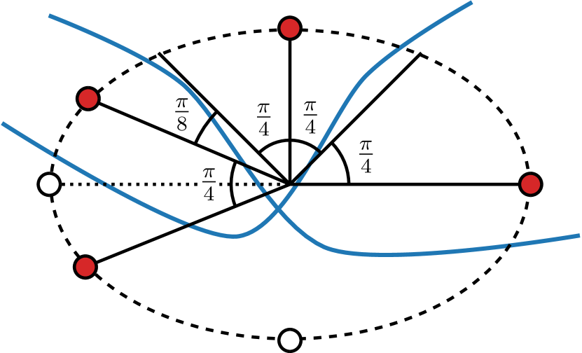
Figure 8: Sketch of the algorithm for finding the inputs to the BCM: four arbitrary initial phase space coordinates representative of the four regions associated with the NHIM. Instead of naively choosing coordinates on two right-angled axes (empty circles), an ellipse enclosing the geometric cross is constructed. The first point (filled circle on right hand side) is selected arbitrarily at coordinates with angle $\alpha=0$. Subsequent coordinates are found by incrementing $\alpha$ in steps of $\Delta\alpha=\pi/4$ (solid lines), and confirming that said point satisfies the condition of a new region. If a region is skipped—e. g. as shown in the dotted line—the increment $\Delta\alpha$ is temporarily reduced until a point in the region in between is found.

Interestingly, even a given geometric cross is not entirely free of substructures. Instead, it features a fractal-like set of crossing manifolds in its close proximity. Since these additional structures are extremely thin, however, they do not hinder the BCM from finding the desired geometric cross coordinates up to the desired precision which maybe be even smaller than the width of substructures.

Appendix B Decay rates methods

B.1 Ensemble method

The conceptually simplest method for calculating decay rates $k_{\mathrm{e}}$ is by means of propagation of an ensemble. In analogy to Ref. Feldmaier et al. (2019b) we first identify a line segment parallel to the unstable manifold that satisfies the property: it lies on the reactant side between the stable manifold and the DS at a distance that is small enough to allow for linear response and large enough to suppress numerical instability. At $t=t_{0}$, an ensemble of particles is placed on this line and propagated in time to yield a time-dependent reactant population $N_{\mathrm{R}}(t;t_{0})$.

In the second major step, one can obtain a reaction rate constant $k_{\mathrm{e}}$ by fitting an exponential decay $N_{\mathrm{R}}(t;t_{0})\propto\exp[-k_{\mathrm{e}}(t-t_{0})]$ to the reactant population Pechukas (1981); Chandler (1978); Miller et al. (1983); Hänggi et al. (1990); Connors (1990); Upadhyay (2006). This, however, is not possible in all systems—and, in particular, in the two-saddle system being investigated here—because the decay in $N_{\mathrm{R}}(t;t_{0})$ can be nonexponential. Instead, we use the more general approach described in Ref. Feldmaier et al. (2019b), which involves examining the instantaneous decays

$$k_{\mathrm{e}}(t;t_{0})=-\frac{1}{N_{\mathrm{R}}(t;t_{0})}\derivative{t}N_{\mathrm{R}}(t;t_{0})\,\text{.}$$ (4)

An analogous definition has been used in Ref. Lehmann et al. (2000a) for escape rates over a potential barrier.

B.2 Local manifold analysis

In general, the approach described above is computationally expensive since a lot of particles have to be propagated. This led us to develop a second method, called the LMA, for obtaining instantaneous reaction rates purely from the geometry of the stable and unstable manifolds in phase space. If the slopes of the stable and unstable manifolds $\mathcal{W}_{\mathrm{s}}$ and $\mathcal{W}_{\mathrm{u}}$ at time $t$ are given by $\Delta v_{x}^{\mathrm{s}}(t)/\Delta x$ and $\Delta v_{x}^{\mathrm{u}}(t)/\Delta x$ then the instantaneous rate $k_{\mathrm{m}}(t)$ can be written as their difference Feldmaier et al. (2019b),

$$k_{\mathrm{m}}(t)=\frac{\Delta v_{x}^{\mathrm{u}}(t)-\Delta v_{x}^{\mathrm{s}}(t)}{\Delta x}\,\text{.}$$ (5)

This allows for the calculation of $k_{\mathrm{m}}(t)$ independently at different times $t$, making it easy to compute in parallel.

B.3 Floquet method

Last, average decay rates $k_{\mathrm{F}}$ can also be obtained directly using a Floquet stability analysis Craven et al. (2014); Feldmaier et al. (2019b) that was seen earlier to lead to accurate rates in reactions with a time-dependent barrier. While this method is the computationally cheapest, it cannot yield instantaneous rates.

To obtain the time-independent rate constant $k_{\mathrm{F}}$ for a given trajectory on the NHIM, we can linearize the equations of motion using the Jacobian

$$J(t)=\matrixquantity(0&1\\ -\derivative*[2]{V(x,t)}{x}&0)\,\text{.}$$ (6)

By integrating the differential equation

$$\derivative{\sigma(t)}{t}=J(t)\sigma(t)\mbox{\quad with\quad}\sigma(0)=\mathbb{1}\,\text{,}$$ (7)

one obtains the system’s fundamental matrix $\sigma(t)$. When considering trajectories with period $T$, $M=\sigma(T)$ is called the monodromy matrix. Its eigenvalues $m_{\mathrm{u}}$ and $m_{\mathrm{s}}$, termed Floquet multipliers, can be used to determine the Floquet rate constant

$$k_{\mathrm{F}}=\frac{1}{T}\quantity(\ln\absolutevalue{m_{\mathrm{u}}}-\ln\absolutevalue{m_{\mathrm{s}}})\,\text{.}$$ (8)

Appendix C Possible errors for the discontinuous DS in Fig. 5(b)

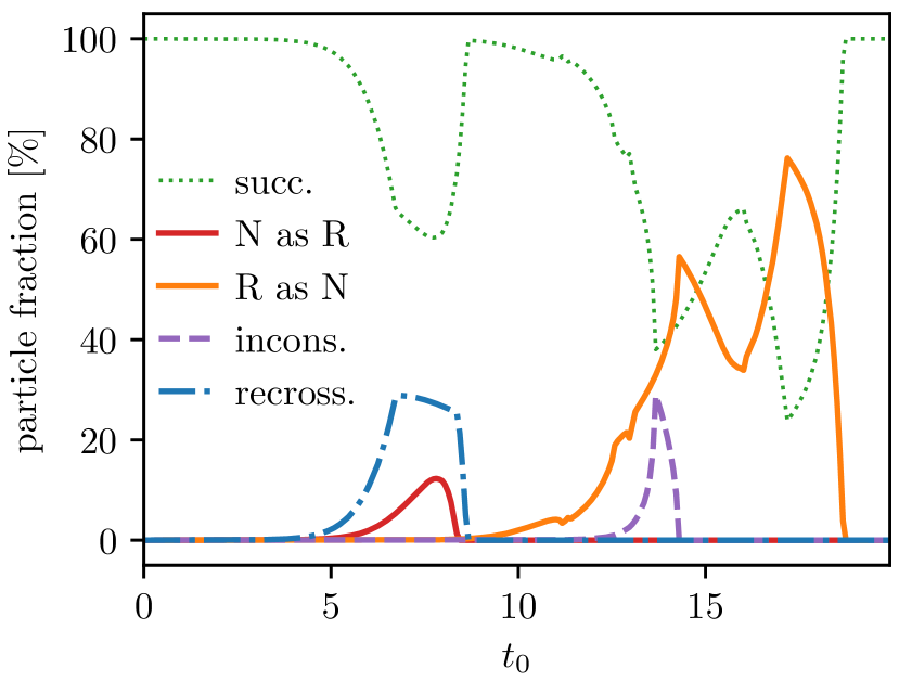
Figure 9: Fraction of trajectories with (see text) and without (labeled “succ.”) errors as a function of time $t_{0}$ for the discontinuous DS from Fig 5.

There are multiple ways in which a discontinuous DS can show errors for a trajectory:

(i) A nonreactive trajectory is classified as reactive (labeled “N as R” in Fig. 9). This can happen when a reactant enters the central region between the saddles while the DS is located near the left saddle. If this happens shortly before the DS jumps to the right, the particle can get reflected at the right barrier and leave the central region on the reactant side.

(ii) A reactive trajectory is classified as nonreactive (labeled “R as N” in Fig. 9). This can happen when a reactant enters the central region while the DS is located near the right saddle. The DS can then jump discontinuously over the particle to the left saddle—which is not counted as a crossing—before the particle leaves the central region to the right as a product.

(iii) The classification is thus inconsistent (labeled “incons.” in Fig. 9). This can happen, e. g., when a reactant enters the central region while the DS is located near the right saddle, and leaves it again to the reactant side while the DS is near the left saddle. As a result, a backward reaction is recorded even though the particle started as a reactant. Similarly, it is possible to detect two forward reactions over the same DS without an intermediate backward reaction. It is unclear which reaction is to be counted as the real one.

(iv) The trajectory crosses the DS multiple times, i. e., it exhibits recrossings (labeled “recross.” in Fig. 9). This can happen when a particle enters and leaves the central region on the reactant side while the DS is near the left saddle, resulting in two crossings.

The distributions of the errors that arise from the discontinuous DS originating from recrossing and misclassification are shown in Fig. 9. The sum of these errors gives rise to that reported in Fig. 5 for this DS.

References

- Truhlar et al. (1983) D. G. Truhlar, W. L. Hase, and J. T. Hynes, J. Phys. Chem. 87, 2664 (1983), doi:10.1021/j100238a003.
- Marcus (1992) R. A. Marcus, Science 256, 1523 (1992), doi:10.1126/science.256.5063.1523.
- Truhlar et al. (1996) D. G. Truhlar, B. C. Garrett, and S. J. Klippenstein, J. Phys. Chem. 100, 12771 (1996), doi:10.1021/jp953748q.
- Komatsuzaki and Berry (2001) T. Komatsuzaki and R. S. Berry, Proc. Natl. Acad. Sci. U.S.A. 98, 7666 (2001), doi:10.1073/pnas.131627698.
- Anslyn and Dougherty (2006) E. V. Anslyn and D. A. Dougherty, Modern Physical Organic Chemistry (University Science Books, Mill Valley, CA, 2006).
- Harper et al. (2011) M. R. Harper, K. M. Van Geem, S. P. Pyl, G. B. Marin, and W. H. Green, Combustion and Flame 158, 16 (2011), doi:10.1016/j.combustflame.2010.06.002.
- Chill et al. (2014) S. T. Chill, J. Stevenson, V. Ruehle, C. Shang, P. Xiao, J. D. Farrell, D. J. Wales, and G. Henkelman, Journal of Chemical Theory and Computation 10, 5476 (2014), doi:10.1021/ct5008718.
- Kramer et al. (2015) Z. C. Kramer, B. K. Carpenter, G. S. Ezra, and S. Wiggins, J. Phys. Chem. A 119, 6611 (2015), doi:10.1021/acs.jpca.5b02834.
- Chen et al. (2017) B. Chen, R. Hoffmann, and R. Cammi, Angew. Chem., Int. Ed. 56, 11126 (2017), doi:10.1002/anie.201705427.
- Miller (1968) W. H. Miller, J. Chem. Phys. 48, 1651 (1968), doi:10.1063/1.1668891.
- Miller (1979) W. H. Miller, J. Phys. Chem. 83, 960 (1979), doi:10.1021/j100471a015.
- Doering and Gadoua (1992) C. R. Doering and J. C. Gadoua, Phys. Rev. Lett. 69, 2318 (1992), doi:10.1103/PhysRevLett.69.2318.
- Maddox (1992) J. Maddox, Nature (London) 359, 771 (1992), doi:10.1038/359771a0.
- Lehmann et al. (2000a) J. Lehmann, P. Reimann, and P. Hänggi, Phys. Rev. Lett. 84, 1639 (2000a), doi:10.1103/PhysRevLett.84.1639.
- Lehmann et al. (2000b) J. Lehmann, P. Reimann, and P. Hänggi, Phys. Rev. E 62, 6282 (2000b), doi:10.1103/PhysRevE.62.6282.
- Lehmann et al. (2003) J. Lehmann, P. Reimann, and P. Hänggi, Phys. Status Solidi B 237, 53 (2003), doi:10.1002/pssb.200301774.
- Van den Broeck (1993) C. Van den Broeck, Phys. Rev. E 47, 4579 (1993), doi:10.1103/PhysRevE.47.4579.
- Hänggi (1994) P. Hänggi, Chem. Phys. 180, 157 (1994), doi:10.1016/0301-0104(93)E0422-R.
- Shepherd and Hernandez (2001) T. D. Shepherd and R. Hernandez, J. Chem. Phys. 115, 2430 (2001), doi:10.1063/1.1386422.
- Shepherd and Hernandez (2002a) T. D. Shepherd and R. Hernandez, J. Chem. Phys. 117, 9227 (2002a), doi:10.1063/1.1516590.
- Shepherd and Hernandez (2002b) T. D. Shepherd and R. Hernandez, J. Phys. Chem. B 106, 8176 (2002b), doi:10.1021/jp020620h.
- Moix et al. (2004) J. M. Moix, T. D. Shepherd, and R. Hernandez, J. Phys. Chem. B 108, 19476 (2004), doi:10.1021/jp046629w.
- Vogelaere and Boudart (1955) R. D. Vogelaere and M. Boudart, J. Chem. Phys. 23, 1236 (1955), doi:10.1063/1.1742248.
- Miller (1976) W. H. Miller, J. Chem. Phys. 65, 2216 (1976), doi:10.1063/1.433379.
- Pollak et al. (1980) E. Pollak, M. S. Child, and P. Pechukas, J. Chem. Phys. 72, 1669 (1980), doi:10.1063/1.439276.
- Carpenter (2005) B. K. Carpenter, “Potential energy surfaces and reaction dynamics,” in Reactive Intermediate Chemistry (John Wiley & Sons, New York, 2005) Chap. 21, pp. 925–960.
- Pechukas (1976) P. Pechukas, Dynamics of Molecular Collisions, edited by W. H. Miller, Vol. 2 (Plenum, New York, 1976) Chap. 6, pp. 269–322.
- Pechukas (1981) P. Pechukas, Annu. Rev. Phys. Chem. 32, 159 (1981), doi:10.1146/annurev.pc.32.100181.001111.
- Pollak and Pechukas (1979) E. Pollak and P. Pechukas, J. Chem. Phys. 70, 325 (1979), doi:10.1063/1.437194.
- Rehbein and Carpenter (2011) J. Rehbein and B. K. Carpenter, Phys. Chem. Chem. Phys. 13, 20906 (2011), doi:10.1039/C1CP22565K.
- Collins et al. (2013) P. Collins, B. K. Carpenter, G. S. Ezra, and S. Wiggins, J. Chem. Phys. 139, 154108 (2013), doi:10.1063/1.4825155.
- Craven and Hernandez (2016) G. T. Craven and R. Hernandez, Phys. Chem. Chem. Phys. 18, 4008 (2016), doi:10.1039/c5cp06624g.
- Junginger et al. (2017) A. Junginger, L. Duvenbeck, M. Feldmaier, J. Main, G. Wunner, and R. Hernandez, J. Chem. Phys. 147, 064101 (2017), doi:10.1063/1.4997379.
- Glasstone et al. (1941) S. Glasstone, K. J. Laidler, and H. Eyring, The Theory of Rate Processes: The Knetics of Chemical Reactions, Viscosity, Diffusion and Electrochemical Phenomena (McGraw-Hill, New York, 1941).
- Fukui (1970) K. Fukui, J. Phys. Chem. 74, 4161 (1970), doi:10.1021/j100717a029.
- Kato and Fukui (1976) S. Kato and K. Fukui, J. Am. Chem. Soc. 98, 6395 (1976), doi:https://doi.org/10.1021/ja00436a061.
- Eyring (1935) H. Eyring, J. Chem. Phys. 3, 107 (1935), doi:10.1063/1.1749604.
- Wigner (1937) E. P. Wigner, J. Chem. Phys. 5, 720 (1937), doi:10.1063/1.1750107.
- Feldmaier et al. (2019a) M. Feldmaier, P. Schraft, R. Bardakcioglu, J. Reiff, M. Lober, M. Tschöpe, A. Junginger, J. Main, T. Bartsch, and R. Hernandez, J. Phys. Chem. B 123, 2070 (2019a), doi:10.1021/acs.jpcb.8b10541.
- Lichtenberg and Liebermann (1982) A. J. Lichtenberg and M. A. Liebermann, Regular and Stochastic Motion (Springer, New York, 1982).
- Hernandez and Miller (1993) R. Hernandez and W. H. Miller, Chem. Phys. Lett. 214, 129 (1993), doi:10.1016/0009-2614(93)90071-8.
- Hernandez (1993) R. Hernandez, Ph.D. thesis, University of California, Berkeley, CA (1993).
- Ott (2002) E. Ott, Chaos in Dynamical Systems, 2nd ed. (Cambridge University Press, Cambridge, England, 2002).
- Wiggins (2013) S. Wiggins, Normally Hyperbolic Invariant Manifolds in Dynamical Systems, Vol. 105 (Springer Science & Business Media, New York, 2013).
- Komatsuzaki and Berry (1999) T. Komatsuzaki and R. S. Berry, Phys. Chem. Chem. Phys. 1, 1387 (1999), doi:10.1039/A809424A.
- Li et al. (2006a) C.-B. Li, A. Shoujiguchi, M. Toda, and T. Komatsuzaki, Few-Body Systems 38, 173 (2006a).
- Li et al. (2006b) C.-B. Li, A. Shoujiguchi, M. Toda, and T. Komatsuzaki, Phys. Rev. Lett. 97, 028302 (2006b), doi:10.1103/PhysRevLett.97.028302.
- Li et al. (2009) C.-B. Li, M. Toda, and T. Komatsuzaki, J. Chem. Phys. 130, 124116 (2009), doi:10.1063/1.3079819.
- Mendoza and Mancho (2010) C. Mendoza and A. M. Mancho, Phys. Rev. Lett. 105, 038501 (2010), doi:10.1103/PhysRevLett.105.038501.
- Mancho et al. (2013) A. M. Mancho, S. Wiggins, J. Curbelo, and C. Mendoza, Commun. Nonlinear Sci. Numer. Simul. 18, 3530 (2013), doi:10.1016/j.cnsns.2013.05.002.
- Craven and Hernandez (2015) G. T. Craven and R. Hernandez, Phys. Rev. Lett. 115, 148301 (2015), doi:10.1103/PhysRevLett.115.148301.
- Junginger and Hernandez (2016) A. Junginger and R. Hernandez, J. Phys. Chem. B 120, 1720 (2016), doi:10.1021/acs.jpcb.5b09003.
- Bardakcioglu et al. (2018) R. Bardakcioglu, A. Junginger, M. Feldmaier, J. Main, and R. Hernandez, Phys. Rev. E 98, 032204 (2018), doi:10.1103/PhysRevE.98.032204.
- Feldmaier et al. (2019b) M. Feldmaier, R. Bardakcioglu, J. Reiff, J. Main, and R. Hernandez, J. Chem. Phys. 151, 244108 (2019b), doi:10.1063/1.5127539.
- Feldmaier et al. (2020) M. Feldmaier, J. Reiff, R. M. Benito, F. Borondo, J. Main, and R. Hernandez, J. Chem. Phys. 153, 084115 (2020), doi:10.1063/5.0015509.
- Craven et al. (2014) G. T. Craven, T. Bartsch, and R. Hernandez, J. Chem. Phys. 141, 041106 (2014), doi:10.1063/1.4891471.
- Hammond (1955) G. S. Hammond, J. Am. Chem. Soc. 77, 334 (1955), doi:10.1021/ja01607a027.
- Gezelter and Miller (1995) J. D. Gezelter and W. H. Miller, J. Chem. Phys. 103, 7868 (1995), doi:10.1063/1.470204.
- Ulusoy et al. (2013) I. S. Ulusoy, J. F. Stanton, and R. Hernandez, J. Phys. Chem. A 117, 7553 (2013), doi:10.1021/jp402322h.
- Maugière et al. (2014) F. A. L. Maugière, P. Collins, G. Ezra, S. C. Farantos, and S. Wiggins, Theor. Chem. Acta 133, 1507 (2014), doi:10.1007/s00214-014-1507-4.
- Ulusoy and Hernandez (2014) I. S. Ulusoy and R. Hernandez, Theor. Chem. Acc. 133, 1528 (2014), doi:10.1007/s00214-014-1528-z.
- Párraga et al. (2013) H. Párraga, F. J. Arranz, R. M. Benito, and F. Borondo, J. Chem. Phys. 139, 194304 (2013), doi:10.1063/1.4830102.
- Párraga et al. (2018) H. Párraga, F. J. Arranz, R. M. Benito, and F. Borondo, J. Phys. Chem. A 122, 3433 (2018), doi:10.1021/acs.jpca.8b00113.
- Chandler (1978) D. Chandler, J. Chem. Phys. 68, 2959 (1978), doi:10.1063/1.436049.
- Miller et al. (1983) W. H. Miller, S. D. Schwartz, and J. W. Tromp, J. Chem. Phys. 79, 4889 (1983), doi:10.1063/1.445581.
- Hänggi et al. (1990) P. Hänggi, P. Talkner, and M. Borkovec, Rev. Mod. Phys. 62, 251 (1990), doi:10.1103/RevModPhys.62.251, and references therein.
- Connors (1990) K. A. Connors, Chemical Kinetics: The Study of Reaction Rates in Solution (Wiley-VCH, Weinham, Germany, 1990).
- Upadhyay (2006) S. K. Upadhyay, Chemical Kinetics and Reaction Dynamics (Springer, Amsterdam, 2006).