Abstract

We consider the approximation of manifold-valued functions by embedding the manifold into a higher dimensional space, applying a vector-valued approximation operator and projecting the resulting vector back to the manifold. It is well known that the approximation error for manifold-valued functions is close to the approximation error for vector-valued functions. This is not true anymore if we consider the derivatives of such functions. In our paper we give pre-asymptotic error bounds for the approximation of the derivative of manifold-valued function. In particular, we provide explicit constants that depend on the reach of the embedded manifold.

Keywords: nonlinear approximation, manifold-valued functions, embedded manifolds

1 Introduction

Approximating functions $f\colon\Omega\to\mathcal{M}$ with values in some $D$-dimensional Riemannian manifold $\mathcal{M}$ has attracted lots of interest during the last years. The central challenge is that with $\mathcal{M}$ not being linear, the function spaces over $\Omega$ with values in $\mathcal{M}$ are not linear as well and hence, all the well established linear approximation methods do not have a straight forward generalization to manifold-valued functions.

One successful approach to manifold-valued approximation is to consider the problem locally. Either one maps the function values locally to some linear approximation space or one uses local averaging based on the geodesic distance. These approaches allow to generalize subdivision schemes [32, 33, 9, 10, 29], moving least squares [12], quasi-interpolation [11] or splines [30] to the manifold-valued setting.

A different approach is to embed the manifold $\mathcal{M}$ into some higher dimensional linear space $\mathbb{R}^{d}$ by a map $\mathcal{E}\colon\mathcal{M}\to\mathbb{R}^{d}$. Note, that according to Nash’s embedding theorem [21] such a mapping always exists and can be guaranteed to be locally isometric provided the dimension $d$ is at least $D(3D+11)/2$, where $D$ denotes the dimension of $\mathcal{M}$. Embedding based approximation methods can be summarized as follows

1. Transfer $f\in C(\Omega,\mathcal{M}$) via the embedding $\mathcal{E}$ into the linear function space $C(\Omega,\mathbb{R}^{d})$. Since often a manifold is described by vectors in $\mathbb{R}^{d}$, we will use the notation $f$ for the function in both function spaces.

2. Use a linear approximation operator $I_{\mathbb{R}^{d}}\colon C(\Omega,\mathbb{R}^{d})\to C(\Omega,\mathbb{R}^{d})$ to find an approximant $I_{\mathbb{R}^{d}}f$ in the embedding.

3. Project the resulting $\mathbb{R}^{d}$-valued function back to the manifold $I_{\mathcal{M}}f=P_{\mathcal{M}}\circ(I_{\mathbb{R}^{d}}f)$ using some projection operator $P_{\mathcal{M}}\colon\mathbb{R}^{d}\to\mathcal{M}$.

Because of its generality and simplicity this approach has already been widely investigated [11, 7] and applied [20, 27]. In particular it has been shown in [7] that the approximation order of the embedding based approximation operator $I_{\mathcal{M}}f$ is the same as the approximation order of its linear counterpart $I_{\mathbb{R}^{d}}$. It is important to note, that the projection operator $P_{\mathcal{M}}$ is in general only defined in some neighborhood $U\supset\mathcal{M}$ of the manifold. Hence, the pre-asymptotic behavior of the approximation operator $I_{\mathcal{M}}$ strongly depends on the size of this neighborhood which is directly related to the so-called reach of the embedded manifold.

The aim of this paper is to analyze the pre-asymptotic behavior of the approximation operator $I_{\mathcal{M}}$ with respect to the reach of the embedded manifold. While for the error $I_{\mathcal{M}}f-f$ the reach only controls the required linear approximation error $I_{\mathbb{R}^{d}}f-f$ that allows for a meaningful approximation $I_{\mathcal{M}}f$, the situation is completely different for the error of the derivatives $\,\mathrm{d}(I_{\mathcal{M}}f)-\,\mathrm{d}f$. In this case the chain rule has to be used for the derivative $\,\mathrm{d}(I_{\mathcal{M}}f)$ of a concatenation of approximation in $\mathbb{R}^{d}$ and projection on the manifold $\mathcal{M}$. The derivative of the projection on $\mathcal{M}$ leads to pre-asymptotic constants, which depend on the reach of the manifold.

Our paper is organized as follows. In section 2 we will first show some general differential geometric properties of submanifolds of $\mathbb{R}^{d}$. Most importantly, we identify in Lemma 2.1 the projection operator $P_{\mathcal{M}}$ with an orthogonal projection in the normal bundle over the manifold $\mathcal{M}$. This is only possible within some tubular neighborhood of the manifold $\mathcal{M}$ that is controlled by the reach of $\mathcal{M}$. The relationship between the reach of the manifold $\mathcal{M}$ and its curvature or second fundamental form is addressed in section 2.2. In Theorem 2.7 we make use of these relationships to describe the differential of the projection operator $P_{\mathcal{M}}$ in terms of the second fundamental form. In section 2.4 we end up with the main results of this chapter, that is we show in Theorem 2.10 that the derivative $dP_{\mathcal{M}}(\mathbf{\boldsymbol{x}})$ of the projection operator at some point $\mathbf{\boldsymbol{x}}\in\mathbb{R}^{d}$ satisfies a Lipschitz-condition with respect to $\mathbf{\boldsymbol{x}}$. As our Lipschitz bound is with respect to the Euclidean distance in the embedding it is more sharp then the bound reported in [3] that relies on the geodesic distance.

Section 3 is dedicated to manifold-valued approximation. We show that the approach of using a linear approximation operator on an embedded manifold $\mathcal{M}$ in $\mathbb{R}^{d}$ and then projecting back on the manifold inherits the approximation order of the linear approximation. Our main result is stated in Theorem 3.2 and gives a pre-asymptotic bound for the approximation error of the first derivative that relies exclusively on the reach of the embedded manifold. This result is illustrated in Theorem 3.4 for a specific approximation operator, the Fourier partial sum operator.

In the final section 4 we consider two real world examples for approximating manifold valued data. The first example deals with functions from the two-sphere into the two-dimensional projective space that describe the dependency between the propagation direction and the polarization directions of seismic waves. The second example is from crystallographic texture analysis where the local alignment of the atom lattice is described by a map with values in the quotient $\mathrm{SO}(3)/\mathcal{S}$ of the rotation group $\mathrm{SO}(3)$ modulo some finite symmetry group $\mathcal{S}$. The derivative of this map has important connections microscopic and macroscopic material properties.

2 Submanifolds

In this section we will consider smooth compact Riemannian submanifolds $\mathcal{M}$ of $\mathbb{R}^{d}$. We will show some differential geometric properties of submanifolds as well as some estimations for the projection $P_{\mathcal{M}}$ and the differential of this projection. We will use these results for estimating some approximation errors in section 3.

2.1 The Projection Operator

Throughout our work we denote by $\mathcal{M}\subset\mathbb{R}^{d}$ a smooth compact Riemannian submanifold of $\mathbb{R}^{d}$. For every point $\mathbf{\boldsymbol{m}}\in\mathcal{M}$ we denote the tangent space $T_{\mathbf{\boldsymbol{m}}}\mathcal{M}$ as well as the normal space $N_{\mathbf{\boldsymbol{m}}}\mathcal{M}$. Furthermore, we denote by $P_{\mathcal{M}}\colon\mathbb{R}^{d}\to\mathcal{M}$ the projection operator onto $\mathcal{M}$ defined as the solution of the minimization problem

$$P_{\mathcal{M}}(\mathbf{\boldsymbol{x}})=\operatorname*{argmin}_{\mathbf{\boldsymbol{m}}\in\mathcal{M}}\left\lVert\smash{\mathbf{\boldsymbol{x}}-\mathbf{\boldsymbol{m}}}\right\rVert_{2}.$$ (2.1)

In general, this minimization problem does not posses a unique solution for every $\mathbf{\boldsymbol{x}}\in\mathbb{R}^{d}$, since there is an ambiguity to which branch of the manifold the point should be attributed. However, if we restrict the domain of the definition of $P_{\mathcal{M}}$ to some open neighborhood $U\subset\mathbb{R}^{d}$ of $\mathcal{M}$ uniqueness can be granted.

In order to find such a neighborhood $U$ we define on the normal bundle

$$N\mathcal{M}=\{(\mathbf{\boldsymbol{m}},\mathbf{\boldsymbol{v}})\in\mathbb{R}^{d}\times\mathbb{R}^{d}:\mathbf{\boldsymbol{m}}\in\mathcal{M},\mathbf{\boldsymbol{v}}\in N_{\mathbf{\boldsymbol{m}}}\mathcal{M}\}$$

of $\mathcal{M}$ the smooth map

$$E\colon N\mathcal{M}\to\mathbb{R}^{d},\quad E(\mathbf{\boldsymbol{m}},\mathbf{\boldsymbol{v}})=\mathbf{\boldsymbol{m}}+\mathbf{\boldsymbol{v}},$$

that maps every normal space $N_{\mathbf{\boldsymbol{m}}}\mathcal{M}$ to an affine linear subspace through $\mathbf{\boldsymbol{m}}\in\mathbb{R}^{d}$. Since we assumed $\mathcal{M}$ to be compact and smooth, there exist a maximum constant $\tau>0$ such that the mapping $E$ restricted to the open subset

$$V=\{(\mathbf{\boldsymbol{m}},\mathbf{\boldsymbol{v}})\in N\mathcal{M}:\left\lVert\smash{\mathbf{\boldsymbol{v}}}\right\rVert_{2}<\tau\}$$

of the normal bundle is injective, cf. [17, 6.24]. Setting $U=E(V)$ defines the so-called tubular neighborhood of $\mathcal{M}$ and the restriction $E\colon V\to U$ becomes a diffeomorphism. The constant $\tau$ is commonly called reach and its inverse $1/\tau$ is the condition number of the manifold. The reach $\tau$ is affected by two factors: the curvature of the manifold and the width of the narrowest bottleneck-like structure of $\mathcal{M}$, which quantifies how far $\mathcal{M}$ is from being self-intersecting. An estimate on the relationship between the reach and the curvature of the manifold $\mathcal{M}$ will be given in Lemma 2.4.

Using the mapping $E$ we may now give an explicit definition of the projection operator $P_{\mathcal{M}}$.

Lemma 2.1.

Let $\mathbf{\boldsymbol{u}}\in U$ and let $\pi\colon N\mathcal{M}\to\mathcal{M}$, $(\mathbf{\boldsymbol{m}},\mathbf{\boldsymbol{n}})\mapsto\mathbf{\boldsymbol{m}}$ be the canonical projection operator. Then

$$P_{\mathcal{M}}(\mathbf{\boldsymbol{u}})=\pi\circ E^{-1}(\mathbf{\boldsymbol{u}})$$

is the unique solution of the minimization problem (2.1).

Proof.

Let $\mathbf{\boldsymbol{u}}\in U$ and $P_{\mathcal{M}}(\mathbf{\boldsymbol{u}})=\mathbf{\boldsymbol{m}}\in\mathcal{M}$. We show that $\mathbf{\boldsymbol{u}}-\mathbf{\boldsymbol{m}}\in N_{\mathbf{\boldsymbol{m}}}\mathcal{M}$. We assume the opposite and decompose $\mathbf{\boldsymbol{u}}-\mathbf{\boldsymbol{m}}$ in one part in $N_{\mathbf{\boldsymbol{m}}}\ M$ and a part $\mathbf{\boldsymbol{t}}$ in $T_{\mathbf{\boldsymbol{m}}}M$. Then there is a curve $\gamma(s)$ in $\mathcal{M}$ with $\gamma(0)=\mathbf{\boldsymbol{m}}$ and $\dot{\gamma}(0)=\mathbf{\boldsymbol{t}}$. If we go along this curve, we obtain for sufficient small $\epsilon>0$ that $\mathbf{\boldsymbol{u}}-\gamma(\epsilon)<\mathbf{\boldsymbol{u}}-\gamma(0)=\mathbf{\boldsymbol{u}}-\mathbf{\boldsymbol{m}}$. That is a contradiction to the definition of $P_{\mathcal{M}}$. Since the projection $P_{\mathcal{M}}$ should be unique, we have to show that $\pi\circ E^{-1}$ is also unique. For that reason we assume that for $\mathbf{\boldsymbol{u}}\in U$ there holds $\pi\circ E^{-1}=\mathbf{\boldsymbol{m}}\in\mathcal{M}$ and $\pi\circ E^{-1}=\mathbf{\boldsymbol{m}}^{\prime}\in\mathcal{M}$. This would imply $\mathbf{\boldsymbol{u}}=\mathbf{\boldsymbol{m}}+\mathbf{\boldsymbol{v}}=\mathbf{\boldsymbol{m}}^{\prime}+\mathbf{\boldsymbol{v}}^{\prime}$ with $\mathbf{\boldsymbol{v}}\in N_{\mathbf{\boldsymbol{m}}}\mathcal{M}$ and $\mathbf{\boldsymbol{v}}\in N_{\mathbf{\boldsymbol{m}}^{\prime}}\mathcal{M}$. That is a contradiction to the uniqueness of $E^{-1}$ in the tubular neighborhood $U$. ∎

Let us illustrate this by a simple example.

Example 2.2.

Let the manifold $\mathcal{M}$ be the $(d-1)$-dimensional unit sphere, embedded in $\mathbb{R}^{d}$. These manifolds can be described by

$$\mathbb{S}^{d-1}=\left\{\mathbf{\boldsymbol{x}}\in\mathbb{R}^{d}:\|\mathbf{\boldsymbol{x}}\|_{2}=1\right\}.$$

The projection $P_{\mathbb{S}^{d-1}}$ easily reads

$$P_{\mathbb{S}^{d-1}}:\mathbb{R}^{d}\backslash\{\mathbf{\boldsymbol{0}}\}\rightarrow\mathbb{S}^{d-1},\quad\quad P_{\mathbb{S}^{d-1}}(\mathbf{\boldsymbol{x}})=\frac{\mathbf{\boldsymbol{x}}}{\|\mathbf{\boldsymbol{x}}\|_{2}}.$$

This map is well-defined and smooth.

2.2 Curvature and Reach of Submanifolds

For any point $\mathbf{\boldsymbol{m}}\in\mathcal{M}\subset\mathbb{R}^{d}$ on the manifold we can decompose $\mathbb{R}^{d}$ as the direct sum $\mathbb{R}^{d}=T_{\mathbf{\boldsymbol{m}}}\mathcal{M}\oplus N_{\mathbf{\boldsymbol{m}}}\mathcal{M}$ of the tangential space $T_{\mathbf{\boldsymbol{m}}}\mathcal{M}$ and the normal space $N_{\mathbf{\boldsymbol{m}}}\mathcal{M}$. Let us denote by $P_{T}\colon\mathbb{R}^{d}\to T_{\mathbf{\boldsymbol{m}}}\mathcal{M}$ and $P_{N}\colon\mathbb{R}^{d}\to N_{\mathbf{\boldsymbol{m}}}\mathcal{M}$ the corresponding orthogonal projections. Then the canonical connection $\nabla$ on $\mathbb{R}^{d}$ defines a connection $\nabla^{\mathcal{M}}$ on $\mathcal{M}$ by

$$\nabla^{\mathcal{M}}_{\mathbf{\boldsymbol{X}}}=P_{T}\nabla_{\mathbf{\boldsymbol{X}}}(P_{T}\mathbf{\boldsymbol{Y}})+P_{N}\nabla_{\mathbf{\boldsymbol{X}}}(P_{N}\mathbf{\boldsymbol{Y}}),$$ (2.2)

where $\mathbf{\boldsymbol{X}}\colon\mathcal{M}\to T\mathcal{M}$ is a tangential and $\mathbf{\boldsymbol{Y}}\colon\mathcal{M}\to\mathbb{R}^{d}$ a general vector field on $\mathcal{M}$.

If $\mathbf{\boldsymbol{Y}}$ is a tangential vector field as well, the first summand $P_{T}\nabla_{\mathbf{\boldsymbol{X}}}(P_{T}\mathbf{\boldsymbol{Y}})=P_{T}\nabla_{\mathbf{\boldsymbol{X}}}\mathbf{\boldsymbol{Y}}$ in (2.2) is just the Levi-Cevita-connection on $\mathcal{M}$, whereas its orthogonal complement

$$\mathord{\mathrm{II}}(\mathbf{\boldsymbol{X}},\mathbf{\boldsymbol{Y}})=P_{N}(\nabla_{\mathbf{\boldsymbol{X}}}\mathbf{\boldsymbol{Y}})$$

is the second fundamental form on $\mathcal{M}$.

We call a vector field $\mathbf{\boldsymbol{Y}}\colon\mathcal{M}\to\mathbb{R}^{d}$ parallel along a curve $\gamma$ if $\nabla^{\mathcal{M}}_{\dot{\gamma}}\mathbf{\boldsymbol{Y}}=0$. For a geodesic $\gamma$ with $\gamma(0)=\mathbf{\boldsymbol{m}}$, $\dot{\gamma}(0)=\mathbf{\boldsymbol{t}}\in T_{\mathbf{\boldsymbol{m}}}\mathcal{M}$ and an arbitrary vector $\mathbf{\boldsymbol{y}}\in T_{\mathbf{\boldsymbol{m}}}\mathcal{M}\oplus N_{\mathbf{\boldsymbol{m}}}\mathcal{M}=\mathbb{R}^{d}$ we shall use the abbreviation

$$\nabla_{\mathbf{\boldsymbol{t}}}\mathbf{\boldsymbol{y}}=\nabla_{\mathbf{\boldsymbol{t}}}\mathbf{\boldsymbol{Y}}(0)$$

where $\mathbf{\boldsymbol{Y}}$ is the parallel transport of the vector $\mathbf{\boldsymbol{y}}$ along the curve $\gamma$.

For a fixed point $\mathbf{\boldsymbol{m}}\in\mathcal{M}$ and a normal direction $\mathbf{\boldsymbol{n}}\in N_{\mathbf{\boldsymbol{m}}}\mathcal{M}$ we define the operator $\mathbf{\boldsymbol{B}}_{\mathbf{\boldsymbol{n}}}\colon T_{\mathbf{\boldsymbol{m}}}\mathcal{M}\to T_{\mathbf{\boldsymbol{m}}}\mathcal{M}$ on the tangent space by

$$\left<\mathbf{\boldsymbol{B}}_{\mathbf{\boldsymbol{n}}}\mathbf{\boldsymbol{x}},\mathbf{\boldsymbol{y}}\right>=\left<\mathbf{\boldsymbol{n}},\nabla_{\mathbf{\boldsymbol{x}}}\mathbf{\boldsymbol{y}}\right>,\quad\mathbf{\boldsymbol{x}},\mathbf{\boldsymbol{y}}\in T_{\mathbf{\boldsymbol{m}}}\mathcal{M}.$$ (2.3)

We may also express $B_{\mathbf{\boldsymbol{n}}}\mathbf{\boldsymbol{x}}$ as the tangential part of the covariant derivative of $\mathbf{\boldsymbol{n}}$ in direction $\mathbf{\boldsymbol{x}}$.

Lemma 2.3.

Let $\mathbf{\boldsymbol{n}}\in N_{\mathbf{\boldsymbol{m}}}\mathcal{M}$ be a normal and $\mathbf{\boldsymbol{x}}\in T_{\mathbf{\boldsymbol{m}}}\mathcal{M}$ a tangential vector. Then

$$\mathbf{\boldsymbol{B}}_{\mathbf{\boldsymbol{n}}}\mathbf{\boldsymbol{x}}=-P_{T}\nabla_{\mathbf{\boldsymbol{x}}}\mathbf{\boldsymbol{n}}.$$

Proof.

Let $\gamma$ be a geodesics in $\mathcal{M}$ with $\gamma(0)=\mathbf{\boldsymbol{m}}$ and $\dot{\gamma}(0)=\mathbf{\boldsymbol{x}}$ and let $\mathbf{\boldsymbol{N}}$ be the parallel transport of $\mathbf{\boldsymbol{n}}$ along $\gamma$. Let furthermore, $\mathbf{\boldsymbol{Y}}$ be an arbitrary tangent vector field parallel along $\gamma$. Then we have

$$0=\frac{\,\mathrm{d}}{\,\mathrm{d}s}\langle\mathbf{\boldsymbol{N}}(s),\mathbf{\boldsymbol{Y}}(s)\rangle|_{s=0}=\langle\nabla_{\mathbf{\boldsymbol{x}}}\mathbf{\boldsymbol{N}}(0),\mathbf{\boldsymbol{Y}}(0)\rangle+\langle\mathbf{\boldsymbol{N}}(0),\mathbf{\boldsymbol{\nabla}}_{\mathbf{\boldsymbol{x}}}\mathbf{\boldsymbol{Y}}(0)\rangle.$$

This yields

$$\langle\mathbf{\boldsymbol{B}}_{\mathbf{\boldsymbol{n}}}\mathbf{\boldsymbol{x}},\mathbf{\boldsymbol{y}}\rangle=\langle\mathbf{\boldsymbol{n}},\nabla_{\mathbf{\boldsymbol{x}}}\mathbf{\boldsymbol{y}}\rangle=-\langle\nabla_{\mathbf{\boldsymbol{x}}}\mathbf{\boldsymbol{n}},\mathbf{\boldsymbol{y}}\rangle.$$

Since the vector field $\mathbf{\boldsymbol{Y}}$ was arbitrary, this yields the assertion. ∎

The operator $\mathbf{\boldsymbol{B}}_{\mathbf{\boldsymbol{n}}}$ describes the extrinsic curvature of the manifold in the point $\mathbf{\boldsymbol{m}}$ and the normal direction $\mathbf{\boldsymbol{n}}$. Its norm is bounded by the condition number $\frac{1}{\tau}$ of $\mathcal{M}$. More precisely the following result is shown in [22, Proposition 6.1].

Lemma 2.4.

Let $\tau$ be the reach of $\mathcal{M}$, $\mathbf{\boldsymbol{m}}\in\mathcal{M}$ be an arbitrary point on the manifold and $\mathbf{\boldsymbol{n}}\in N_{\mathbf{\boldsymbol{m}}}\mathcal{M}$ be a normal vector. Then the operator $B_{\mathbf{\boldsymbol{n}}}$ defined in (2.3) is symmetric and bounded by $\frac{1}{\tau}$, i.e., we have for tangential vectors $\mathbf{\boldsymbol{x}},\mathbf{\boldsymbol{y}}\in T_{\mathbf{\boldsymbol{m}}}\mathcal{M}$ the inequality

$$\left<\mathbf{\boldsymbol{B}}_{\mathbf{\boldsymbol{n}}}\mathbf{\boldsymbol{x}},\mathbf{\boldsymbol{y}}\right>\leq\frac{1}{\tau}\left\lVert\smash{\mathbf{\boldsymbol{n}}}\right\rVert\left\lVert\smash{\mathbf{\boldsymbol{x}}}\right\rVert\left\lVert\smash{\mathbf{\boldsymbol{y}}}\right\rVert.$$ (2.4)

The next lemma bounds the covariant derivative of parallel vector fields by the condition number $\frac{1}{\tau}$ of the manifold.

Lemma 2.5.

Let $\mathbf{\boldsymbol{Y}}$ be a parallel vector field along a geodesic $\gamma$ in $\mathcal{M}$. Then its covariant derivative in $\mathbb{R}^{d}$ is bounded by

$$\left\lVert\smash{\nabla_{\dot{\gamma}}\mathbf{\boldsymbol{Y}}}\right\rVert_{2}\leq\tfrac{1}{\tau}\left\lVert\smash{\mathbf{\boldsymbol{Y}}}\right\rVert_{2}\left\lVert\smash{\dot{\gamma}}\right\rVert_{2}.$$

Proof.

Let $\mathbf{\boldsymbol{Y}}=\mathbf{\boldsymbol{T}}+\mathbf{\boldsymbol{N}}$ be the decomposition of $\mathbf{\boldsymbol{Y}}$ into a tangent vector field $\mathbf{\boldsymbol{T}}$ and a normal vector field $\mathbf{\boldsymbol{N}}$. Since $\mathbf{\boldsymbol{Y}}$ is parallel along $\gamma$ we have

$$0=\nabla_{\dot{\gamma}}^{\mathcal{M}}\mathbf{\boldsymbol{Y}}=P_{T}\nabla_{\dot{\gamma}}\mathbf{\boldsymbol{T}}+P_{N}\nabla_{\dot{\gamma}}\mathbf{\boldsymbol{N}}$$

and, hence,

$$\nabla_{\dot{\gamma}}\mathbf{\boldsymbol{Y}}=P_{N}\nabla_{\dot{\gamma}}\mathbf{\boldsymbol{T}}+P_{T}\nabla_{\dot{\gamma}}\mathbf{\boldsymbol{N}}.$$

Let $\mathbf{\boldsymbol{n}}=P_{N}\nabla_{\dot{\gamma}(s)}\mathbf{\boldsymbol{T}}(s)$. Then we obtain by Lemma 2.4

$$\left\lVert\smash{\mathbf{\boldsymbol{n}}}\right\rVert^{2}=\left<\mathbf{\boldsymbol{n}},\nabla_{\dot{\gamma}(s)}\mathbf{\boldsymbol{T}}(s)\right>=\left<\mathbf{\boldsymbol{B}}_{\mathbf{\boldsymbol{n}}}\dot{\gamma}(s),\mathbf{\boldsymbol{T}}(s)\right>\leq\tfrac{1}{\tau}\left\lVert\smash{\dot{\gamma}}\right\rVert\left\lVert\smash{\mathbf{\boldsymbol{n}}}\right\rVert\left\lVert\smash{\mathbf{\boldsymbol{T}}(s)}\right\rVert.$$

For the tangential part we have by Lemma 2.3

$$\left\lVert\smash{P_{T}\nabla_{\dot{\gamma}(s)}\mathbf{\boldsymbol{N}}(s)}\right\rVert_{2}=\left\lVert\smash{\mathbf{\boldsymbol{B}}_{\mathbf{\boldsymbol{N}}(s)}\dot{\gamma}(s)}\right\rVert_{2}\leq\tfrac{1}{\tau}\left\lVert\smash{\dot{\gamma}}\right\rVert\left\lVert\smash{\mathbf{\boldsymbol{N}}(s)}\right\rVert.$$

The assertion follows now from Parsevals inequality. ∎

2.3 The Differential of the Projection Operator.

The differential $\,\mathrm{d}P_{\mathcal{M}}(\mathbf{\boldsymbol{m}})\colon\mathbb{R}^{d}\to T_{\mathbf{\boldsymbol{m}}}\mathcal{M}$ of the projection $P_{\mathcal{M}}\colon\mathbb{R}^{d}\to\mathcal{M}$ is especially easy to compute at points $\mathbf{\boldsymbol{m}}\in\mathcal{M}$ on the manifold. In this case it is simply the linear projection $P_{T_{\mathbf{\boldsymbol{m}}}\mathcal{M}}\colon\mathbb{R}^{d}\to T_{\mathbf{\boldsymbol{m}}}\mathcal{M}$ onto the tangential space attached to $\mathbf{\boldsymbol{m}}$, i.e.

$$\,\mathrm{d}P_{\mathcal{M}}(\mathbf{\boldsymbol{m}})=P_{T_{\mathbf{\boldsymbol{m}}}\mathcal{M}}.$$ (2.5)

We can verify this by observing that for normal vectors $\mathbf{\boldsymbol{n}}\in N_{\mathbf{\boldsymbol{m}}}\mathcal{M}$ we have

$$\,\mathrm{d}P_{\mathcal{M}}(\mathbf{\boldsymbol{m}})\,\mathbf{\boldsymbol{n}}=\lim_{h\to 0}\frac{P_{\mathcal{M}}(\mathbf{\boldsymbol{m}}+h\mathbf{\boldsymbol{n}})-P_{\mathcal{M}}(\mathbf{\boldsymbol{m}})}{h}=\lim_{h\to 0}\frac{\mathbf{\boldsymbol{m}}-\mathbf{\boldsymbol{m}}}{h}=\mathbf{\boldsymbol{0}},$$

while for tangent vectors $\mathbf{\boldsymbol{t}}\in T_{\mathbf{\boldsymbol{m}}}\mathcal{M}$ we obtain

$$\,\mathrm{d}P_{\mathcal{M}}(\mathbf{\boldsymbol{m}})\,\mathbf{\boldsymbol{t}} =\lim_{h\to 0}\frac{P_{\mathcal{M}}(\mathbf{\boldsymbol{m}}+h\mathbf{\boldsymbol{t}})-P_{\mathcal{M}}(\mathbf{\boldsymbol{m}})}{h}=\lim_{h\to 0}\frac{\mathbf{\boldsymbol{m}}+\exp(h\mathbf{\boldsymbol{t}})-\mathbf{\boldsymbol{m}}}{h}$$

$$=\lim_{h\to 0}\frac{\exp(h\mathbf{\boldsymbol{t}})}{h}=\mathbf{\boldsymbol{t}},$$

where $\exp$ denotes the exponential map to the manifold.

The differential $\,\mathrm{d}P_{\mathcal{M}}(\mathbf{\boldsymbol{m}}+\mathbf{\boldsymbol{v}})$, $\mathbf{\boldsymbol{v}}\in N_{\mathbf{\boldsymbol{m}}}\mathcal{M}$ at a point not in the manifold is a little bit more tricky. We start by observing that the tangential $T_{(\mathbf{\boldsymbol{m}},\mathbf{\boldsymbol{v}})}N\mathcal{M}\subset\mathbb{R}^{2d}$ of the normal bundle at a point $(\mathbf{\boldsymbol{m}},\mathbf{\boldsymbol{v}})\in N\mathcal{M}$ is

$$T_{(\mathbf{\boldsymbol{m}},\mathbf{\boldsymbol{v}})}N\mathcal{M} =\{(\mathbf{\boldsymbol{0}},\mathbf{\boldsymbol{n}})\mid\mathbf{\boldsymbol{n}}\in N_{\mathbf{\boldsymbol{m}}}\mathcal{M}\}\oplus\{(\mathbf{\boldsymbol{t}},\nabla_{\mathbf{\boldsymbol{t}}}\mathbf{\boldsymbol{v}})\mid\mathbf{\boldsymbol{t}}\in T_{\mathbf{\boldsymbol{m}}}\mathcal{M}\}$$

$$=\{(\mathbf{\boldsymbol{t}},\mathbf{\boldsymbol{u}})\mid\mathbf{\boldsymbol{t}}\in T_{\mathbf{\boldsymbol{m}}}\mathcal{M},P_{T}\mathbf{\boldsymbol{u}}=\nabla_{\mathbf{\boldsymbol{t}}}\mathbf{\boldsymbol{v}}\}.$$

The following lemma describes the differential $\,\mathrm{d}P_{\mathcal{M}}(\mathbf{\boldsymbol{m}}+\mathbf{\boldsymbol{v}})$.

Lemma 2.6.

Let $\mathbf{\boldsymbol{m}}\in\mathcal{M}$ be an arbitrary point on the manifold $\mathcal{M}$ and $\mathbf{\boldsymbol{v}}\in N_{\mathbf{\boldsymbol{m}}}\mathcal{M}$ be a normal vector with $\left\lVert\smash{\mathbf{\boldsymbol{v}}}\right\rVert_{2}<\tau$, i.e. $\mathbf{\boldsymbol{m}}+\mathbf{\boldsymbol{v}}$ is in the tubular neighborhood of $\mathcal{M}$. Then the derivative $\mathrm{d}P_{\mathcal{M}}(\mathbf{\boldsymbol{m}}+\mathbf{\boldsymbol{v}})$ satisfies for every tangent direction $\mathbf{\boldsymbol{t}}\in T_{\mathbf{\boldsymbol{m}}}\mathcal{M}$,

$$\left(\mathrm{d}P_{\mathcal{M}}(\mathbf{\boldsymbol{m}}+\mathbf{\boldsymbol{v}})\right)\left(\mathbf{\boldsymbol{t}}+\nabla_{\mathbf{\boldsymbol{t}}}\mathbf{\boldsymbol{v}}\right)=\mathbf{\boldsymbol{t}}.$$

while it vanishes for any normal direction $\mathbf{\boldsymbol{n}}\in N_{\mathbf{\boldsymbol{m}}}\mathcal{M}$, i.e.

$$\mathrm{d}P_{\mathcal{M}}(\mathbf{\boldsymbol{m}}+\mathbf{\boldsymbol{v}})\,\mathbf{\boldsymbol{n}}=\mathbf{\boldsymbol{0}}.$$

Proof.

According to Lemma 2.1 we have $P_{\mathcal{M}}=\pi\circ E^{-1}$, where $\pi\colon N\mathcal{M}\to\mathcal{M}$, $(\mathbf{\boldsymbol{m}},\mathbf{\boldsymbol{v}})\mapsto\mathbf{\boldsymbol{m}}$ is the projection operator. Its differential at the point $(\mathbf{\boldsymbol{m}},\mathbf{\boldsymbol{v}})\in N\mathcal{M}$ is the projection

$$\,\mathrm{d}\pi(\mathbf{\boldsymbol{m}},\mathbf{\boldsymbol{v}})\colon T_{(\mathbf{\boldsymbol{m}},\mathbf{\boldsymbol{v}})}N\mathcal{M}\to T_{\mathbf{\boldsymbol{m}}}\mathcal{M},\quad(\mathbf{\boldsymbol{t}},\mathbf{\boldsymbol{u}})\mapsto\mathbf{\boldsymbol{t}}.$$

The differential of the mapping $E\colon N\mathcal{M}\to\mathbb{R}^{d}$ in a point $(\mathbf{\boldsymbol{m}},\mathbf{\boldsymbol{v}})\in N\mathcal{M}$ is given by

$$\,\mathrm{d}E(\mathbf{\boldsymbol{m}},\mathbf{\boldsymbol{v}})\colon T_{(\mathbf{\boldsymbol{m}},\mathbf{\boldsymbol{v}})}N\mathcal{M}\to\mathbb{R}^{d},\quad(\mathbf{\boldsymbol{t}},\mathbf{\boldsymbol{u}})\mapsto\mathbf{\boldsymbol{t}}+\mathbf{\boldsymbol{u}}.$$

Since $\mathbf{\boldsymbol{m}}+\mathbf{\boldsymbol{v}}$ is within the tubular neighborhood of $\mathcal{M}$, $E$ is invertible in some neighborhood of $\mathbf{\boldsymbol{m}}+\mathbf{\boldsymbol{v}}$. Then $\,\mathrm{d}E(\mathbf{\boldsymbol{m}},\mathbf{\boldsymbol{v}})$ is invertible as well and we have for any normal vector $\mathbf{\boldsymbol{n}}\in N_{\mathbf{\boldsymbol{m}}}\mathcal{M}$

$$\,\mathrm{d}E^{-1}(\mathbf{\boldsymbol{m}}+\mathbf{\boldsymbol{v}})\,\mathbf{\boldsymbol{n}}=(\mathbf{\boldsymbol{0}},\mathbf{\boldsymbol{n}})$$

and for any tangent vector $\mathbf{\boldsymbol{t}}\in T_{\mathbf{\boldsymbol{m}}}\mathcal{M}$

$$\,\mathrm{d}E^{-1}(\mathbf{\boldsymbol{m}}+\mathbf{\boldsymbol{v}})\,(\mathbf{\boldsymbol{t}}+\nabla_{\mathbf{\boldsymbol{t}}}\mathbf{\boldsymbol{v}})=(\mathbf{\boldsymbol{t}},\nabla_{\mathbf{\boldsymbol{t}}}\mathbf{\boldsymbol{v}}).$$

Together with the chain rule this implies the assertion. ∎

The image of $\mathrm{d}P_{\mathcal{M}}(\mathbf{\boldsymbol{m}}+\mathbf{\boldsymbol{v}})$ is contained in the tangential space $T_{\mathbf{\boldsymbol{m}}}\mathcal{M}$, especially $\mathrm{d}P_{\mathcal{M}}(\mathbf{\boldsymbol{m}}+\mathbf{\boldsymbol{v}})$ is the projection $P_{T_{\mathbf{\boldsymbol{m}}}\mathcal{M}}$ up to a factor matrix. We will write this linear operator $\mathrm{d}P_{\mathcal{M}}(\mathbf{\boldsymbol{m}}+\mathbf{\boldsymbol{v}})$ in another way, to see the difference to the linear operator $\mathrm{d}P_{\mathcal{M}}(\mathbf{\boldsymbol{m}})$.

Theorem 2.7.

Let $\mathbf{\boldsymbol{m}}\in\mathcal{M}$ be a point on the manifold, let $\mathbf{\boldsymbol{v}}\in N_{\mathbf{\boldsymbol{m}}}\mathcal{M}$ be a normal vector with $\left\lVert\smash{\mathbf{\boldsymbol{v}}}\right\rVert<\tau$ and let $\mathbf{\boldsymbol{B}}_{\mathbf{\boldsymbol{v}}}\colon T_{\mathbf{\boldsymbol{m}}}\mathcal{M}\to T_{\mathbf{\boldsymbol{m}}}\mathcal{M}$ be the symmetric operator defined in (2.3), extended to $\mathbf{\boldsymbol{B}}_{\mathbf{\boldsymbol{v}}}\colon\mathbb{R}^{d}\to\mathbb{R}^{d}$ by $\mathbf{\boldsymbol{B}}_{\mathbf{\boldsymbol{v}}}\mathbf{\boldsymbol{n}}=\mathbf{\boldsymbol{0}}$ for all normal vectors $\mathbf{\boldsymbol{n}}\in N_{\mathbf{\boldsymbol{m}}}\mathcal{M}$. Then the derivative of the projection operator $P_{\mathcal{M}}$ satisfies

$$\mathrm{d}P_{\mathcal{M}}(\mathbf{\boldsymbol{m}}+\mathbf{\boldsymbol{v}})=P_{T_{\mathbf{\boldsymbol{m}}}\mathcal{M}}(\mathbf{\boldsymbol{I}}-\mathbf{\boldsymbol{B}}_{\mathbf{\boldsymbol{v}}})^{-1}=\mathrm{d}P_{\mathcal{M}}(\mathbf{\boldsymbol{m}})-\mathbf{\boldsymbol{B}}_{\mathbf{\boldsymbol{v}}}\left(\mathbf{\boldsymbol{I}}+\mathbf{\boldsymbol{B}}_{\mathbf{\boldsymbol{v}}}\right)^{-1},$$

where $\mathbf{\boldsymbol{I}}\colon\mathbb{R}^{d}\to\mathbb{R}^{d}$ is the identity.

Proof.

Using Lemma 2.6 we obtain for all tangential vectors $\mathbf{\boldsymbol{t}}\in T_{\mathbf{\boldsymbol{m}}}\mathcal{M}$,

$$P_{T_{\mathbf{\boldsymbol{m}}}\mathcal{M}}\mathbf{\boldsymbol{t}} =\mathbf{\boldsymbol{t}}=\left(\mathrm{d}P_{\mathcal{M}}(\mathbf{\boldsymbol{m}}+\mathbf{\boldsymbol{v}})\right)\left(\mathbf{\boldsymbol{t}}+\nabla_{\mathbf{\boldsymbol{t}}}\mathbf{\boldsymbol{v}}\right)$$

$$=\left(\mathrm{d}P_{\mathcal{M}}(\mathbf{\boldsymbol{m}}+\mathbf{\boldsymbol{v}})\right)\left(\mathbf{\boldsymbol{t}}-\mathbf{\boldsymbol{B}}_{\mathbf{\boldsymbol{v}}}\mathbf{\boldsymbol{t}}\right)=\left(\mathrm{d}P_{\mathcal{M}}(\mathbf{\boldsymbol{m}}+\mathbf{\boldsymbol{v}})\right)\left(\mathbf{\boldsymbol{I}}-\mathbf{\boldsymbol{B}}_{\mathbf{\boldsymbol{v}}}\right)\mathbf{\boldsymbol{t}}.$$

and for all normal vectors $\mathbf{\boldsymbol{n}}\in N_{\mathbf{\boldsymbol{m}}}\mathcal{M}$,

$$\mathbf{\boldsymbol{0}}=P_{T_{\mathbf{\boldsymbol{m}}}\mathcal{M}}\mathbf{\boldsymbol{n}}=\left(\mathrm{d}P_{\mathcal{M}}(\mathbf{\boldsymbol{m}}+\mathbf{\boldsymbol{v}})\right)\left(\mathbf{\boldsymbol{I}}-\mathbf{\boldsymbol{B}}_{\mathbf{\boldsymbol{v}}}\right)\mathbf{\boldsymbol{n}}.$$

Consequently, we have

$$P_{T_{\mathbf{\boldsymbol{m}}}\mathcal{M}}=\mathrm{d}P_{\mathcal{M}}(\mathbf{\boldsymbol{m}}+\mathbf{\boldsymbol{v}})\left(\mathbf{\boldsymbol{I}}-\mathbf{\boldsymbol{B}}_{\mathbf{\boldsymbol{v}}}\right).$$

By our assumption and (2.4) we have $\left\lVert\smash{\mathbf{\boldsymbol{B}}_{\mathbf{\boldsymbol{v}}}}\right\rVert\leq\frac{1}{\tau}\left\lVert\smash{\mathbf{\boldsymbol{v}}}\right\rVert<1$ and hence, the operator $\mathbf{\boldsymbol{I}}-\mathbf{\boldsymbol{B}}_{\mathbf{\boldsymbol{v}}}$ is invertible. This yields the first part of the assertion. For the second part we use (2.5) and compute

$$\mathrm{d}P_{\mathcal{M}}(\mathbf{\boldsymbol{m}}+\mathbf{\boldsymbol{v}}) =P_{T_{\mathbf{\boldsymbol{m}}}\mathcal{M}}\left(\mathbf{\boldsymbol{I}}-\mathbf{\boldsymbol{B}}_{\mathbf{\boldsymbol{v}}}\right)^{-1}$$

$$=P_{T_{\mathbf{\boldsymbol{m}}}\mathcal{M}}\left(\mathbf{\boldsymbol{I}}+\mathbf{\boldsymbol{B}}_{\mathbf{\boldsymbol{v}}}\left(\mathbf{\boldsymbol{I}}-\mathbf{\boldsymbol{B}}_{\mathbf{\boldsymbol{v}}}\right)^{-1}\right)$$

$$=\mathrm{d}P_{\mathcal{M}}(\mathbf{\boldsymbol{m}})+P_{T_{\mathbf{\boldsymbol{m}}}\mathcal{M}}\mathbf{\boldsymbol{B}}_{\mathbf{\boldsymbol{v}}}\left(\mathbf{\boldsymbol{I}}-\mathbf{\boldsymbol{B}}_{\mathbf{\boldsymbol{v}}}\right)^{-1}$$

$$=\mathrm{d}P_{\mathcal{M}}(\mathbf{\boldsymbol{m}})+\mathbf{\boldsymbol{B}}_{\mathbf{\boldsymbol{v}}}\left(\mathbf{\boldsymbol{I}}-\mathbf{\boldsymbol{B}}_{\mathbf{\boldsymbol{v}}}\right)^{-1},$$

where the last equality follows from the fact that the image of $\mathbf{\boldsymbol{B}}_{\mathbf{\boldsymbol{n}}}$ is in the tangent space $T_{\mathbf{\boldsymbol{m}}}\mathcal{M}$, so the projection on $T_{\mathbf{\boldsymbol{m}}}\mathcal{M}$ is unnecessary. ∎

We consider again the manifold from example 2.2.

Example 2.8.

For $\mathcal{M}=\mathbb{S}^{d-1}\subset\mathbb{R}^{d}$ any normal vector $\mathbf{\boldsymbol{v}}\in N_{\mathbf{\boldsymbol{m}}}\mathbb{S}^{d-1}$ has the representation $\mathbf{\boldsymbol{v}}=v\,\mathbf{\boldsymbol{m}}$. Let $\{\mathbf{\boldsymbol{t}}_{i}\}_{i=1}^{d-1}\subset T_{\mathbf{\boldsymbol{m}}}\mathbb{S}^{d-1}$ be an orthonormal basis of $T_{m}\mathbb{S}^{d-1}$. Then $\nabla_{\mathbf{\boldsymbol{t}}_{i}}\mathbf{\boldsymbol{m}}=\mathbf{\boldsymbol{t}}_{j}$ and hence

$$\mathbf{\boldsymbol{B}}_{\mathbf{\boldsymbol{v}}}=-v\sum_{i=1}^{d-1}{\mathbf{\boldsymbol{t}}_{i}\mathbf{\boldsymbol{t}}_{i}^{\top}}.$$

By Theorem 2.7 and the orthonormality of $\{\mathbf{\boldsymbol{m}}\}\cap\{\mathbf{\boldsymbol{t}}_{i}\}_{i=1}^{d-1}$ of we obtain for $v>-1$ and $\mathbf{\boldsymbol{x}}=\mathbf{\boldsymbol{m}}+v\mathbf{\boldsymbol{m}}$,

$$\,\mathrm{d}P_{\mathbb{S}^{d-1}}(\mathbf{\boldsymbol{x}})=\frac{1}{1+v}\sum_{i=1}^{d-1}{\mathbf{\boldsymbol{t}}_{i}\mathbf{\boldsymbol{t}}_{i}^{\top}}=\frac{1}{\left\lVert\smash{\mathbf{\boldsymbol{x}}}\right\rVert_{2}}\,\left(\mathbf{\boldsymbol{I}}_{d\times d}-\frac{\mathbf{\boldsymbol{x}}}{\left\lVert\smash{\mathbf{\boldsymbol{x}}}\right\rVert_{2}}\left(\frac{\mathbf{\boldsymbol{x}}}{\left\lVert\smash{\mathbf{\boldsymbol{x}}}\right\rVert_{2}}\right)^{\top}\right).$$

2.4 Deviation of the Projection Operator

In this section we are interested in the change of the derivative $\mathrm{d}P_{\mathcal{M}}(\mathbf{\boldsymbol{m}})$ of the projection operator for small deviations of $\mathbf{\boldsymbol{m}}$. We shall show that for two points $\mathbf{\boldsymbol{m}}$ and $\mathbf{\boldsymbol{z}}$ on $\mathcal{M}$ and $\mathbf{\boldsymbol{v}}\in N_{\mathbf{\boldsymbol{m}}}\mathcal{M}$ with $\left\lVert\smash{\mathbf{\boldsymbol{v}}}\right\rVert_{2}<\tau$ we can bound the difference $\left\lVert\smash{\,\mathrm{d}P_{\mathcal{M}}(\mathbf{\boldsymbol{m}}+\mathbf{\boldsymbol{v}})-\,\mathrm{d}P_{\mathcal{M}}(\mathbf{\boldsymbol{z}})}\right\rVert_{2}$ by a multiple of the Euclidean distance $\left\lVert\smash{\mathbf{\boldsymbol{m}}+\mathbf{\boldsymbol{v}}-\mathbf{\boldsymbol{z}}}\right\rVert_{2}$.

As usual we start with the case that both points are on the manifold. According to [3, Lemma 6] the difference of the differentials is then bounded by

$$\left\lVert\smash{\,\mathrm{d}P_{\mathcal{M}}(\mathbf{\boldsymbol{m}})-\,\mathrm{d}P_{\mathcal{M}}(\mathbf{\boldsymbol{z}})}\right\rVert_{2}\leq\frac{1}{\tau}\,d(\mathbf{\boldsymbol{m}},\mathbf{\boldsymbol{z}}),$$

where $d(\mathbf{\boldsymbol{m}},\mathbf{\boldsymbol{z}})$ denotes the geodesic distance between the points $\mathbf{\boldsymbol{m}},\mathbf{\boldsymbol{z}}\in\mathcal{M}$. If the Euclidean distance between the two points is bounded by $\left\lVert\smash{\mathbf{\boldsymbol{m}}-\mathbf{\boldsymbol{z}}}\right\rVert_{2}\leq 2\tau$ we have by [3, Lemma 3] and the fact that $\arcsin(x)\leq\frac{\pi}{2}x$ for $0\leq x\leq 1$, the following estimate between geodesic distance and Euclidean distance in the embedding

$$d(\mathbf{\boldsymbol{m}},\mathbf{\boldsymbol{z}})\leq\frac{\pi}{2}\left\lVert\smash{\mathbf{\boldsymbol{m}}-\mathbf{\boldsymbol{z}}}\right\rVert_{2},$$ (2.6)

which leads to the local estimate

$$\left\lVert\smash{\,\mathrm{d}P_{\mathcal{M}}(\mathbf{\boldsymbol{m}})-\,\mathrm{d}P_{\mathcal{M}}(\mathbf{\boldsymbol{z}})}\right\rVert_{2}\leq\frac{\pi}{2\tau}\left\lVert\smash{\mathbf{\boldsymbol{m}}-\mathbf{\boldsymbol{z}}}\right\rVert_{2}.$$

In the following Theorem we prove a sharper and global bound for this difference.

Theorem 2.9.

For all $\mathbf{\boldsymbol{m}},\mathbf{\boldsymbol{z}}\in\mathcal{M}$ the difference between the projection operators $P_{T_{\mathbf{\boldsymbol{m}}}\mathcal{M}}$ and $P_{T_{\mathbf{\boldsymbol{z}}}\mathcal{M}}$ onto the respective tangential spaces is bounded by

$$\left\|P_{T_{\mathbf{\boldsymbol{m}}}\mathcal{M}}-P_{T_{\mathbf{\boldsymbol{z}}}\mathcal{M}}\right\|_{2}\leq\frac{1}{\tau}\left\lVert\smash{\mathbf{\boldsymbol{m}}-\mathbf{\boldsymbol{z}}}\right\rVert_{2}.$$

Proof.

First of all we note that for $\left\lVert\smash{\mathbf{\boldsymbol{m}}-\mathbf{\boldsymbol{z}}}\right\rVert_{2}\geq 2\,\tau$ the assertion is immediately satisfied since $\left\|P_{T_{\mathbf{\boldsymbol{m}}}\mathcal{M}}-P_{T_{\mathbf{\boldsymbol{z}}}\mathcal{M}}\right\|_{2}\leq 2$ independently of $\mathbf{\boldsymbol{m}},\mathbf{\boldsymbol{z}}\in\mathcal{M}$. We may therefore assume $\left\lVert\smash{\mathbf{\boldsymbol{m}}-\mathbf{\boldsymbol{z}}}\right\rVert_{2}<2\,\tau$ for the rest of the proof.

In order to estimate the difference between the two projection operators we consider a geodesic $\gamma$ with $\gamma(0)=\mathbf{\boldsymbol{m}}$, $\gamma(t)=\mathbf{\boldsymbol{z}}$ and $\left\lVert\smash{\dot{\gamma}}\right\rVert_{2}=1$. Furthermore, we consider an orthonormal basis $\{\mathbf{\boldsymbol{t}}_{i}\}_{i=1}^{D}$ in $T_{\mathbf{\boldsymbol{m}}}\mathcal{M}$ and an orthonormal basis $\{\mathbf{\boldsymbol{n}}_{j}\}_{j=1}^{d-D}$ in $N_{\mathbf{\boldsymbol{m}}}\mathcal{M}$. The parallel transport of these basis vectors along $\gamma$ defines a rotation $\mathbf{\boldsymbol{R}}\in\mathrm{SO}(d)$ that maps the tangent space $T_{\mathbf{\boldsymbol{m}}}\mathcal{M}$ onto the tangent space $T_{\mathbf{\boldsymbol{z}}}\mathcal{M}$. Using the rotation $\mathbf{\boldsymbol{R}}$ we may rewrite the difference between the projection operators as

$$P_{T_{\mathbf{\boldsymbol{m}}}\mathcal{M}}-P_{T_{\mathbf{\boldsymbol{z}}}\mathcal{M}}=P_{T_{\mathbf{\boldsymbol{m}}}\mathcal{M}}-\mathbf{\boldsymbol{R}}P_{T_{\mathbf{\boldsymbol{m}}}\mathcal{M}}\mathbf{\boldsymbol{R}}^{T}.$$

By Lemma A.1 in the appendix we obtain

$$\left\lVert\smash{P_{T_{\mathbf{\boldsymbol{m}}}\mathcal{M}}-P_{T_{\mathbf{\boldsymbol{z}}}\mathcal{M}}}\right\rVert_{2}=\left\lVert\smash{P_{T_{\mathbf{\boldsymbol{m}}}\mathcal{M}}\mathbf{\boldsymbol{R}}-\mathbf{\boldsymbol{R}}P_{T_{\mathbf{\boldsymbol{z}}}\mathcal{M}}}\right\rVert_{2}\leq\left\lVert\smash{\mathbf{\boldsymbol{I}}-\mathbf{\boldsymbol{R}}}\right\rVert_{2}$$ (2.7)

and hence, it suffices to bound for any normalized $\mathbf{\boldsymbol{x}}\in\mathbb{R}^{d}$

$$\left\lVert\smash{(\mathbf{\boldsymbol{I}}-\mathbf{\boldsymbol{R}})\mathbf{\boldsymbol{x}}}\right\rVert_{2}^{2}=2-2\left<\mathbf{\boldsymbol{x}},\mathbf{\boldsymbol{R}}\mathbf{\boldsymbol{x}}\right>.$$ (2.8)

By definition $\mathbf{\boldsymbol{R}}\mathbf{\boldsymbol{x}}$ is the result of the parallel transport of $\mathbf{\boldsymbol{x}}$ along the curve $\gamma$ in $\gamma(t)=\mathbf{\boldsymbol{z}}$. Let us denote by $\mathbf{\boldsymbol{X}}(s)$ the parallel transport of $\mathbf{\boldsymbol{x}}$ along $\gamma$ for all times $s\in[0,t]$. Viewing $s\mapsto\mathbf{\boldsymbol{X}}(s)$ as a curve on $\mathbb{S}^{d-1}$ with velocity bounded according to Lemma 2.5 by $\left\lVert\smash{\dot{\mathbf{\boldsymbol{X}}}(s)}\right\rVert=\left\lVert\smash{\nabla_{\dot{\gamma}(s)}\mathbf{\boldsymbol{X}}(s)}\right\rVert_{2}\leq\frac{1}{\tau}$, we conclude that

$$\angle(\mathbf{\boldsymbol{X}}(\eta),\mathbf{\boldsymbol{X}}(\xi))\leq\frac{1}{\tau}|\eta-\xi|,\quad\eta,\xi\in[0,t].$$ (2.9)

Since $\gamma$ is a geodesic we can set in (2.9), $\mathbf{\boldsymbol{X}}=\dot{\gamma}$. As $\left|\eta-\xi\right|\leq t$ and $t$ is the geodesic distance between $\mathbf{\boldsymbol{z}}$ and $\mathbf{\boldsymbol{m}}$ we can use (2.6) and our assumption $\left\lVert\smash{\mathbf{\boldsymbol{m}}-\mathbf{\boldsymbol{z}}}\right\rVert_{2}<2\tau$ to bound the right hand side of (2.9) by

$$\angle(\dot{\gamma}(\xi),\dot{\gamma}(\eta))\leq\frac{1}{\tau}\left|\eta-\xi\right|\leq\frac{t}{\tau}\leq\frac{\pi}{2\tau}\left\lVert\smash{\mathbf{\boldsymbol{z}}-\mathbf{\boldsymbol{m}}}\right\rVert_{2}\leq\pi.$$

Making use of the monotonicity of the cosine this implies

$$\cos\angle(\dot{\gamma}(\xi),\dot{\gamma}(\eta))>\cos\tfrac{\xi-\eta}{\tau},\quad\xi,\eta\in[0,t].$$ (2.10)

Considering again the general vector field $\mathbf{\boldsymbol{X}}$ we use (2.9) and (2.10) to bound (2.8) by

$$2-2\left<\mathbf{\boldsymbol{X}}(0),\mathbf{\boldsymbol{X}}(t)\right> =2-2\,\cos(\angle(\mathbf{\boldsymbol{X}}(0),\mathbf{\boldsymbol{X}}(t)))$$

$$\leq 2-2\,\cos\tfrac{t}{\tau}=\frac{1}{\tau^{2}}\int_{0}^{t}\int_{0}^{t}\cos\tfrac{\xi-\eta}{\tau}\,\mathrm{d}\eta\,\mathrm{d}\xi$$

$$\leq\frac{1}{\tau^{2}}\int_{0}^{t}\int_{0}^{t}\cos\angle(\dot{\gamma}(\xi),\dot{\gamma}(\eta))\,\mathrm{d}\eta\,\mathrm{d}\xi$$

$$=\frac{1}{\tau^{2}}\int_{0}^{t}\int_{0}^{t}\langle\dot{\gamma}(\xi),\dot{\gamma}(\eta)\rangle\,\mathrm{d}\eta\,\mathrm{d}\xi=\frac{1}{\tau^{2}}\left\lVert\smash{\mathbf{\boldsymbol{m}}-\mathbf{\boldsymbol{z}}}\right\rVert_{2}^{2}.$$

In combination with (2.7) and (2.8) this proves

$$\left\|P_{T_{\mathbf{\boldsymbol{m}}}\mathcal{M}}-P_{T_{\mathbf{\boldsymbol{z}}}\mathcal{M}}\right\|_{2}\leq\frac{1}{\tau}\left\lVert\smash{\mathbf{\boldsymbol{m}}-\mathbf{\boldsymbol{z}}}\right\rVert_{2}.\qed$$

Using the example of the unit circle it can be easily verified that our new bound is sharp.

So far we bounded the variation of the projection operator for points on the manifold. For the general case that only one point is on the manifold we have the following result.

Theorem 2.10.

Let $\mathbf{\boldsymbol{m}},\mathbf{\boldsymbol{z}}\in\mathcal{M}$ and $\mathbf{\boldsymbol{v}}\in N_{\mathbf{\boldsymbol{m}}}\mathcal{M}$ with $\left\lVert\smash{\mathbf{\boldsymbol{v}}}\right\rVert_{2}<\tau$. Then

$$\left\lVert\smash{\mathrm{d}P_{\mathcal{M}}(\mathbf{\boldsymbol{m}}+\mathbf{\boldsymbol{v}})-\mathrm{d}P_{\mathcal{M}}(\mathbf{\boldsymbol{z}})}\right\rVert_{2} \leq\frac{1}{\tau}\left\lVert\smash{\mathbf{\boldsymbol{m}}-\mathbf{\boldsymbol{z}}}\right\rVert_{2}+\frac{1}{\tau-\left\lVert\smash{\mathbf{\boldsymbol{v}}}\right\rVert_{2}}\left\lVert\smash{\mathbf{\boldsymbol{v}}}\right\rVert_{2}$$

$$\leq\left(\frac{2}{\tau}+\frac{1}{\tau-\left\lVert\smash{\mathbf{\boldsymbol{v}}}\right\rVert_{2}}\right)\left\lVert\smash{\mathbf{\boldsymbol{m}}+\mathbf{\boldsymbol{v}}-\mathbf{\boldsymbol{z}}}\right\rVert_{2}.$$

Proof.

Using Theorem 2.7 and Theorem 2.9 we find

$$\left\lVert\smash{\mathrm{d}P_{M}(\mathbf{\boldsymbol{m}}+\mathbf{\boldsymbol{v}})-\mathrm{d}P_{M}(\mathbf{\boldsymbol{z}})}\right\rVert_{2} \leq\left\lVert\smash{\mathrm{d}P_{M}(\mathbf{\boldsymbol{m}}+\mathbf{\boldsymbol{v}})-\mathrm{d}P_{M}(\mathbf{\boldsymbol{m}})}\right\rVert_{2}+\left\lVert\smash{P_{T_{\mathbf{\boldsymbol{m}}}\mathcal{M}}-P_{T_{\mathbf{\boldsymbol{z}}}\mathcal{M}}}\right\rVert_{2}$$

$$\leq\left\lVert\smash{\mathbf{\boldsymbol{B}}_{\mathbf{\boldsymbol{v}}}\left(\mathbf{\boldsymbol{I}}+\mathbf{\boldsymbol{B}}_{\mathbf{\boldsymbol{v}}}\right)^{-1}}\right\rVert_{2}+\tfrac{1}{\tau}\left\lVert\smash{\mathbf{\boldsymbol{m}}-\mathbf{\boldsymbol{z}}}\right\rVert_{2}.$$

From Lemma 2.4 we know that $\left\lVert\smash{\mathbf{\boldsymbol{B}}_{\mathbf{\boldsymbol{v}}}}\right\rVert\leq\frac{\left\lVert\smash{\mathbf{\boldsymbol{v}}}\right\rVert_{2}}{\tau}<1$. This allows us to bound the second term by

$$\left\lVert\smash{\mathbf{\boldsymbol{B}}_{\mathbf{\boldsymbol{v}}}\left(\mathbf{\boldsymbol{I}}+\mathbf{\boldsymbol{B}}_{\mathbf{\boldsymbol{v}}}\right)^{-1}}\right\rVert_{2}\leq\frac{\left\lVert\smash{\mathbf{\boldsymbol{B}}_{\mathbf{\boldsymbol{v}}}}\right\rVert}{1-\left\lVert\smash{\mathbf{\boldsymbol{B}}_{\mathbf{\boldsymbol{v}}}}\right\rVert}\leq\frac{\left\lVert\smash{\mathbf{\boldsymbol{v}}}\right\rVert_{2}}{\tau-\left\lVert\smash{\mathbf{\boldsymbol{v}}}\right\rVert_{2}},$$

which implies the first inequality of the theorem

$$\left\lVert\smash{\mathrm{d}P_{M}(\mathbf{\boldsymbol{m}}+\mathbf{\boldsymbol{v}})-\mathrm{d}P_{M}(\mathbf{\boldsymbol{z}})}\right\rVert_{2}\leq\frac{1}{\tau}\left\lVert\smash{\mathbf{\boldsymbol{m}}-\mathbf{\boldsymbol{z}}}\right\rVert_{2}+\frac{1}{\tau-\left\lVert\smash{\mathbf{\boldsymbol{v}}}\right\rVert_{2}}\left\lVert\smash{\mathbf{\boldsymbol{v}}}\right\rVert_{2}.$$ (2.11)

Since $\left\lVert\smash{\mathbf{\boldsymbol{v}}}\right\rVert_{2}<\tau$ the point $\mathbf{\boldsymbol{m}}+\mathbf{\boldsymbol{v}}$ is within the tubular neighborhood of $\mathcal{M}$ and, hence $\left\lVert\smash{\mathbf{\boldsymbol{v}}}\right\rVert_{2}\leq\left\lVert\smash{\mathbf{\boldsymbol{m}}+\mathbf{\boldsymbol{v}}-\mathbf{\boldsymbol{z}}}\right\rVert_{2}$. Together with the triangle inequality this gives us $\left\lVert\smash{\mathbf{\boldsymbol{m}}-\mathbf{\boldsymbol{z}}}\right\rVert_{2}\leq 2\left\lVert\smash{\mathbf{\boldsymbol{m}}+\mathbf{\boldsymbol{v}}-\mathbf{\boldsymbol{z}}}\right\rVert_{2}$. Including these two inequalities into (2.11) we obtain the assertion. ∎

We observe that the constants in Theorem 2.10 become large if either the reach of the manifold becomes small or the point $\mathbf{\boldsymbol{m}}+\mathbf{\boldsymbol{v}}$ is close to the boundary of the tubular neighborhood of $\mathcal{M}$.

3 Manifold-valued Approximation

In this section we generalize arbitrary approximation operators for vector valued functions to approximation operators for manifold-valued functions. To this end we consider for an arbitrary domain $\Omega$ a generic approximation operator $I_{\mathbb{R}^{d}}\colon C(\Omega,\mathbb{R}^{d})\rightarrow C(\Omega,\mathbb{R}^{d})$. For an embedded manifold $\mathcal{M}\subset\mathbb{R}^{d}$ with reach $\tau$ and projection operator

$$P_{\mathcal{M}}\colon U\to\mathcal{M},\quad U=\{\mathbf{\boldsymbol{y}}\in\mathbb{R}^{d}\mid\min_{\mathbf{\boldsymbol{m}}\in\mathcal{M}}\left\lVert\smash{\mathbf{\boldsymbol{y}}-\mathbf{\boldsymbol{m}}}\right\rVert<\tau\},$$

we define the approximation operator $I_{\mathcal{M}}\colon C(\Omega,\mathcal{M})\to C(\Omega,\mathcal{M})$ for manifold-valued functions as

$$I_{\mathcal{M}}f=P_{\mathcal{M}}\circ I_{\mathbb{R}^{d}}f.$$

It is important to note that $I_{\mathcal{M}}$ is not defined for all functions $f\in C(\Omega,\mathcal{M})$, but only for those for which $I_{\mathbb{R}^{d}}f(x)$ is within the reach of the manifold $\mathcal{M}$, i.e., $\left\lVert\smash{f(\mathbf{\boldsymbol{x}})-I_{\mathbb{R}^{d}}f(x)}\right\rVert_{2}\leq\tau$ for all $\mathbf{\boldsymbol{x}}\in\Omega$.

It is straight forward to see that operator $I_{\mathcal{M}}$ has the same order of approximation as $I_{\mathbb{R}^{d}}$, c.f. [7].

Theorem 3.1.

Let $f\in C(\Omega,\mathcal{M})$ be a continuous $\mathcal{M}$-valued function such that for all $\mathbf{\boldsymbol{x}}\in\Omega$, $I_{\mathbb{R}^{d}}f(\mathbf{\boldsymbol{x}})$ is contained in the reach of $\mathcal{M}$. We then have for all $\mathbf{\boldsymbol{x}}\in\Omega$

$$\left\lVert\smash{I_{\mathcal{M}}f(\mathbf{\boldsymbol{x}})-f(\mathbf{\boldsymbol{x}})}\right\rVert_{2}\leq 2\,\left\lVert\smash{I_{\mathbb{R}^{d}}f(\mathbf{\boldsymbol{x}})-f(\mathbf{\boldsymbol{x}})}\right\rVert_{2}.$$ (3.1)

Proof.

Since $f$ has function values on $\mathcal{M}$, it follows from the definition of $P_{\mathcal{M}}$ in equation (2.1) for all $\mathbf{\boldsymbol{x}}\in\Omega$ that

$$\left\|I_{\mathcal{M}}f(\mathbf{\boldsymbol{x}})-I_{\mathbb{R}^{d}}f(\mathbf{\boldsymbol{x}})\right\|_{2}\leq\left\|f(\mathbf{\boldsymbol{x}})-I_{\mathbb{R}^{d}}f(\mathbf{\boldsymbol{x}})\right\|_{2}.$$

Because of the triangle inequality and the definition of $I_{\mathcal{M}}$ we have

$$\left\lVert\smash{I_{\mathcal{M}}f(\mathbf{\boldsymbol{x}})-f(\mathbf{\boldsymbol{x}})}\right\rVert_{2}\leq\left\lVert\smash{I_{\mathcal{M}}f(\mathbf{\boldsymbol{x}})-I_{\mathbb{R}^{d}}f(\mathbf{\boldsymbol{x}})}\right\rVert_{2}+\left\lVert\smash{I_{\mathbb{R}^{d}}f(\mathbf{\boldsymbol{x}})-f(\mathbf{\boldsymbol{x}})}\right\rVert_{2},\quad\mathbf{\boldsymbol{x}}\in\Omega.\qed$$

As we will see later, considering the error of the differential, things become more complicated.

3.1 Approximation Order of the Differential

In this section we are interested in the approximation error $\left\lVert\smash{\,\mathrm{d}I_{\mathcal{M}}f-\,\mathrm{d}f}\right\rVert_{2}$ between the differential of the manifold-valued approximation $\,\mathrm{d}I_{\mathcal{M}}f$ and the original differential $\,\mathrm{d}f$. To this end we assume from now on that both, $f\colon\Omega\to\mathbb{R}^{d}$ and the vector-valued approximation $\tilde{f}=I_{\mathbb{R}^{d}}f$, are differentiable.

While the error bound for $I_{\mathcal{M}}f$ is independent of the geometry of the manifold $\mathcal{M}$, we will see that this is not true for the differential $\,\mathrm{d}I_{\mathcal{M}}f$ of the manifold-valued approximation. Moreover, it is not sufficient to ensure that $\tilde{f}$ is contained in the reach of $\mathcal{M}$, but instead, it must be bounded away from the reach by some positive constant.

Theorem 3.2.

Let $\tau$ be the reach of the manifold $\mathcal{M}$, $\varepsilon<\tau$ and $f\in C^{1}(\Omega,\mathcal{M})$, such that $\tilde{f}(\mathbf{\boldsymbol{x}})=I_{\mathbb{R}^{d}}f(\mathbf{\boldsymbol{x}})$ satisfies for all $\mathbf{\boldsymbol{x}}\in\Omega$,

$$\left\lVert\smash{f(\mathbf{\boldsymbol{x}})-\tilde{f}(\mathbf{\boldsymbol{x}})}\right\rVert_{2}\leq\varepsilon$$

and, consequently, is contained in the $\varepsilon$-tubular neighborhood of $\mathcal{M}$. Then we have for all $\mathbf{\boldsymbol{x}}\in\Omega$ the following upper bound on the approximation error of the differential $\,\mathrm{d}I_{\mathcal{M}}f$,

$$\begin{split}\left\lVert\smash{\,\mathrm{d}I_{\mathcal{M}}f(\mathbf{\boldsymbol{x}})-\,\mathrm{d}\,f(\mathbf{\boldsymbol{x}})}\right\rVert_{2}\leq\left\lVert\smash{\,\mathrm{d}\tilde{f}(\mathbf{\boldsymbol{x}})-\,\mathrm{d}f(\mathbf{\boldsymbol{x}})}\right\rVert_{2}+C\left\lVert\smash{f(\mathbf{\boldsymbol{x}})-\tilde{f}(\mathbf{\boldsymbol{x}})}\right\rVert_{2}\end{split}$$ (3.2)

where $C$ is given by

$$C=\left(\frac{2}{\tau}+\frac{1}{\tau-\varepsilon}\right)\left(\left\lVert\smash{\,\mathrm{d}\tilde{f}(\mathbf{\boldsymbol{x}})-\,\mathrm{d}f(\mathbf{\boldsymbol{x}})}\right\rVert_{2}+\left\lVert\smash{\,\mathrm{d}f(\mathbf{\boldsymbol{x}})}\right\rVert_{2}\right).$$

Proof.

By the chain rule we obtain for all $\mathbf{\boldsymbol{x}}\in\Omega$,

$$\,\mathrm{d}I_{\mathcal{M}}f(\mathbf{\boldsymbol{x}})=\mathrm{d}P_{\mathcal{M}}(\tilde{f}(\mathbf{\boldsymbol{x}}))\circ\,\mathrm{d}\tilde{f}(\mathbf{\boldsymbol{x}})$$

and from $P_{\mathcal{M}}f=f$,

$$\,\mathrm{d}f(\mathbf{\boldsymbol{x}})=\,\mathrm{d}(P_{\mathcal{M}}f)(\mathbf{\boldsymbol{x}})=\mathrm{d}P_{\mathcal{M}}(f(\mathbf{\boldsymbol{x}}))\circ\,\mathrm{d}f(\mathbf{\boldsymbol{x}}).$$

Using the expansion

$$\,\mathrm{d}(I_{\mathcal{M}}f)(\mathbf{\boldsymbol{x}})-\,\mathrm{d}f(\mathbf{\boldsymbol{x}})= \mathrm{d}P_{\mathcal{M}}(\tilde{f}(\mathbf{\boldsymbol{x}}))\circ\,\mathrm{d}\tilde{f}(\mathbf{\boldsymbol{x}})-\mathrm{d}P_{\mathcal{M}}(f(\mathbf{\boldsymbol{x}}))\circ\,\mathrm{d}f(\mathbf{\boldsymbol{x}})$$

$$= (\mathrm{d}P_{\mathcal{M}}(\tilde{f}(\mathbf{\boldsymbol{x}}))-\mathrm{d}P_{\mathcal{M}}(f(\mathbf{\boldsymbol{x}})))\circ\,\mathrm{d}\tilde{f}(\mathbf{\boldsymbol{x}})$$

$$+\mathrm{d}P_{\mathcal{M}}f(\mathbf{\boldsymbol{x}})\circ(\,\mathrm{d}\tilde{f}(\mathbf{\boldsymbol{x}})-\,\mathrm{d}f(\mathbf{\boldsymbol{x}}))$$

we conclude that

$$\left\lVert\smash{\,\mathrm{d}I_{\mathcal{M}}f(\mathbf{\boldsymbol{x}})-\,\mathrm{d}f(\mathbf{\boldsymbol{x}})}\right\rVert_{2}\leq \left\lVert\smash{\mathrm{d}P_{\mathcal{M}}(\tilde{f}(\mathbf{\boldsymbol{x}}))-\mathrm{d}P_{\mathcal{M}}(f(\mathbf{\boldsymbol{x}}))}\right\rVert_{2}\left\lVert\smash{\,\mathrm{d}\tilde{f}(\mathbf{\boldsymbol{x}})}\right\rVert_{2}$$

$$+\left\lVert\smash{\mathrm{d}P_{\mathcal{M}}(f(\mathbf{\boldsymbol{x}}))}\right\rVert_{2}\left\lVert\smash{\,\mathrm{d}\tilde{f}(\mathbf{\boldsymbol{x}})-\,\mathrm{d}f(\mathbf{\boldsymbol{x}})}\right\rVert_{2}.$$

Since $f(\mathbf{\boldsymbol{x}})\in\mathcal{M}$ and $\left\lVert\smash{f(\mathbf{\boldsymbol{x}})-\tilde{f}(\mathbf{\boldsymbol{x}})}\right\rVert_{2}<\varepsilon$ we have by Theorem 2.10

$$\left\lVert\smash{\mathrm{d}P_{\mathcal{M}}(\tilde{f}(\mathbf{\boldsymbol{x}}))-\mathrm{d}P_{\mathcal{M}}(f(\mathbf{\boldsymbol{x}}))}\right\rVert\leq\left(\frac{2}{\tau}+\frac{1}{\tau-\varepsilon}\right)\left\lVert\smash{f(\mathbf{\boldsymbol{x}})-\tilde{f}(\mathbf{\boldsymbol{x}})}\right\rVert_{2}.$$

Together with the fact that $\left\lVert\smash{\mathrm{d}P_{\mathcal{M}}f(\mathbf{\boldsymbol{x}})}\right\rVert_{2}=1$ we obtain

$$\left\lVert\smash{\,\mathrm{d}(I_{\mathcal{M}}f)(\mathbf{\boldsymbol{x}})-\,\mathrm{d}f(\mathbf{\boldsymbol{x}})}\right\rVert_{2}\leq \left\lVert\smash{f(\mathbf{\boldsymbol{x}})-\tilde{f}(\mathbf{\boldsymbol{x}})}\right\rVert_{2}\left(\frac{2}{\tau}+\frac{1}{\tau-\varepsilon}\right)\left\lVert\smash{\,\mathrm{d}\tilde{f}(\mathbf{\boldsymbol{x}})}\right\rVert_{2}$$

$$+\left\lVert\smash{\,\mathrm{d}\tilde{f}(\mathbf{\boldsymbol{x}})-\,\mathrm{d}f(\mathbf{\boldsymbol{x}})}\right\rVert_{2}.$$

This implies the assertion by triangle inequality. ∎

Asymptotically, as $\left\lVert\smash{f(\mathbf{\boldsymbol{x}})-\tilde{f}(\mathbf{\boldsymbol{x}})}\right\rVert_{2}\to 0$ we have $C\to\frac{3}{\tau}\left\lVert\smash{\,\mathrm{d}f(x)}\right\rVert_{2}$. Since for most approximation methods the decay of the differential $\left\lVert\smash{\,\mathrm{d}f(\mathbf{\boldsymbol{x}})-\,\mathrm{d}\tilde{f}(\mathbf{\boldsymbol{x}})}\right\rVert_{2}$ is one order slower than the decay of $\left\lVert\smash{f(\mathbf{\boldsymbol{x}})-\tilde{f}(\mathbf{\boldsymbol{x}})}\right\rVert_{2}$, we conclude that the right hand bound in (3.2) is dominated by the first summand and, hence, the approximation error of the differential $\,\mathrm{d}I_{\mathcal{M}}f$ of the manifold-valued approximant coincides asymptotically with the approximation error of the vector-valued approximant, as it was already reported in [7]. However, the pre-asymptotic behavior depends strongly on the reach of the embedding of the manifold $\mathcal{M}$.

3.2 Fourier Interpolation

In this section we want to illustrate Theorem 3.2 using Fourier-Interpolation as the approximation operator $I_{\mathbb{R}^{d}}$. More precisely, we define for a function $f\in C(\mathbb{T},\mathbb{R}^{d})$ on the torus $\mathbb{T}$ the Fourier partial sum

$$I_{\mathbb{R}^{d}}f(t)=S_{n}f(t)=\sum_{k=-n}^{n}c_{k}(f)e^{2\pi ikt}$$

with the vector-valued Fourier coefficients

$$c_{k}(f)=\int_{0}^{1}f(x)e^{-2\pi ikx}\,\mathrm{d}{x}.$$

The Fourier-Interpolation satisfies the following well known approximation inequalities, cf. [26].

Theorem 3.3.

Let $r\in\mathbb{N}$ with $r\geq 2$ and $f\in C^{r}(\mathbb{T},\mathbb{R}^{d})$. Then

$$\left\lVert\smash{f(x)-S_{n}f(x)}\right\rVert_{2} \leq\frac{\sqrt{2d}}{(2\pi)^{r}}\,\frac{\sqrt{n}}{n^{r}}\,\left\lVert\smash{f^{(r)}}\right\rVert_{L^{2}(\mathbb{T}),2},$$

$$\left\lVert\smash{\,\mathrm{d}f(x)-\,\mathrm{d}(S_{n}f)(x)}\right\rVert_{2} \leq\frac{\sqrt{2d}}{(2\pi)^{r-1}}\,\frac{\sqrt{n}}{n^{r-1}}\,\left\lVert\smash{f^{(r)}}\right\rVert_{L^{2}(\mathbb{T}),2},$$

with the norm $\left\lVert\smash{f}\right\rVert_{L^{2}(\mathbb{T}),2}^{2}=\int_{\mathbb{T}}\left\lVert\smash{f(x)}\right\rVert_{2}^{2}\,\mathrm{d}x.$

Proof.

The first bound can be found in [4, Theorem 4.3]. The second bound follows from $\,\mathrm{d}(S_{n}f)=S_{n}(\,\mathrm{d}f)$ and the fact that the regularity of $\,\mathrm{d}f$ is one less than the regularity of $f$. The factor $\sqrt{d}$ comes from the fact that the function $f$ maps in the d-dimensional space. ∎

In [26, Theorem 1.39] a similar bound for the $L^{\infty}(\mathbb{T})$-norm can be found. Using the Fourier partial sum operator as the approximation operator $I_{\mathbb{R}^{d}}$ Theorem 3.2 becomes the following.

Theorem 3.4.

Let $\mathcal{M}\subset\mathbb{R}^{d}$ be a submanifold with reach $\tau>0$ and $f\in C^{r}(\mathbb{T},\mathcal{M})$ an $r\geq 2$ times differentiable function with values in $\mathcal{M}$. Let, furthermore, $\varepsilon<\tau$ be an auxiliary constant and the bandwidth $n$ of the Fourier partial sum $S_{n}f$ at least such that $\left\lVert\smash{f(x)-S_{n}f(x)}\right\rVert_{2}\leq\varepsilon$ for all $x\in\mathbb{T}$, i.e.,

$$n^{r-\tfrac{1}{2}}\geq\frac{C_{1}\left\lVert\smash{f^{(r)}}\right\rVert_{L^{2}(\mathbb{T}),2}}{\varepsilon}\text{ with }C_{1}=\frac{\sqrt{2d}}{(2\pi)^{r}}.$$ (3.3)

Then the projection $P_{\mathcal{M}}\circ S_{n}f$ of the Fourier partial sum satisfies for all $x\in\mathbb{T}$,

$$\left\|P_{\mathcal{M}}\circ S_{n}f(x)-f(x)\right\|_{2} \leq 2\,C_{1}\,n^{\tfrac{1}{2}-r}\,\left\lVert\smash{f^{(r)}}\right\rVert_{L^{2}(\mathbb{T}),2},$$ (3.4)

whereas for its differential $\,\mathrm{d}(P_{\mathcal{M}}\circ S_{n}f)$ we obtain

$$\begin{split}\left\|\,\mathrm{d}(P_{\mathcal{M}}\circ S_{n}f)(x)-\,\mathrm{d}f(x)\right\|_{2}&\leq 2\pi\,C_{1}\,\,n^{\tfrac{3}{2}-r}\,\left\lVert\smash{f^{(r)}}\right\rVert_{L^{2}(\mathbb{T}),2}\\ &+C_{2}\,n^{\tfrac{1}{2}-r}\,\left\lVert\smash{f^{(r)}}\right\rVert_{L^{2}(\mathbb{T}),2}^{2},\end{split}$$ (3.5)

with the constant

$$C_{2}=C_{1}\,(\tfrac{2}{\tau}+\tfrac{1}{\tau-\varepsilon})\,(1+2\pi\,C_{1}^{2}\,n^{\frac{3}{2}-r}).$$

Proof.

Together with Theorem 3.3 condition (3.3) ensures that

$$\left\lVert\smash{f(x)-S_{n}f(x)}\right\rVert_{2}\leq\varepsilon<\tau,\quad x\in\mathbb{T}$$

and, hence, $S_{n}f(x)$ has distance less than the reach to $\mathcal{M}$ for all $x\in\mathbb{T}$. This allows us to apply Theorem 3.1 in conjunction with Theorem 3.3 to conclude (3.4).

For the approximation error of the derivative we have by Theorem 3.2

$$\left\lVert\smash{\,\mathrm{d}(P_{\mathcal{M}}\circ S_{n}f)(x)-\,\mathrm{d}f(x)}\right\rVert_{2}\leq\left\lVert\smash{\,\mathrm{d}(S_{n}f)(x)-\,\mathrm{d}f(x)}\right\rVert_{2}+C\left\lVert\smash{S_{n}f(x)-f(x)}\right\rVert_{2}$$

with

$$C=\left(\tfrac{\tau}{2}+\tfrac{1}{\tau-\varepsilon}\right)\,\left(\left\lVert\smash{\,\mathrm{d}(S_{n}f)(x)-\,\mathrm{d}f(x)}\right\rVert_{2}+\left\lVert\smash{\,\mathrm{d}f(x)}\right\rVert_{2}\right).$$

Together with Theorem 3.3 this yields

$$\left\lVert\smash{\,\mathrm{d}(P_{\mathcal{M}}\circ S_{n}f)(x)-\,\mathrm{d}f(x)}\right\rVert_{2}\leq 2\pi\,C_{1}\,n^{\frac{3}{2}-r}\,\left\lVert\smash{f^{(r)}}\right\rVert_{L^{2}(\mathbb{T}),2}+C\,C_{1}\,n^{\frac{1}{2}-r}\,\left\lVert\smash{f^{(r)}}\right\rVert_{L^{2}(\mathbb{T}),2}$$

and

$$C \leq(\tfrac{\tau}{2}+\tfrac{1}{\tau-\varepsilon})\,(2\pi\,C_{1}\,n^{\frac{3}{2}-r}\left\lVert\smash{f^{(r)}}\right\rVert_{L^{2}(\mathbb{T}),2}+\left\lVert\smash{\,\mathrm{d}f(x)}\right\rVert_{2})$$

$$\leq(\tfrac{\tau}{2}+\tfrac{1}{\tau-\varepsilon})\,(2\pi\,C_{1}\,n^{\frac{3}{2}-r}+1)\left\lVert\smash{f^{(r)}}\right\rVert_{L^{2}(\mathbb{T}),2},$$

where we have used the fact that $\left\lVert\smash{\,\mathrm{d}f(x)}\right\rVert_{2}\leq\left\lVert\smash{f^{(r)}}\right\rVert_{L^{2}(\mathbb{T}),2}$ for periodic functions. Setting

$$C_{2}=C_{1}(\tfrac{\tau}{2}+\tfrac{1}{\tau-\varepsilon})(1+2\pi\,C_{1}\,n^{\frac{3}{2}-r})$$

yields the assertion.

∎

Since for $n\to\infty$ we have $C_{2}\to C_{1}(\frac{2}{\tau}+\frac{1}{\tau-\varepsilon})$. Theorem 3.4 states that the approximation order of the differential of the manifold-valued Fourier partial sum operator coincides with the approximation order of the vector-valued operator. In the preasymptotic setting, however, also the second summand with the faster rate $n^{\frac{1}{2}-r}$ is relevant. The constant of this second summand becomes large if the point-wise approximation error is close to the reach $\tau$ of the embedding.

4 Examples

In this section we apply our findings to two real world examples of manifold-valued approximation. Both examples are related to the analysis of crystalline materials. In the first example we consider functions that relate propagation directions of waves to polarization directions and in the second example we consider functions that relate points within crystalline specimen to the local orientation of its crystal lattice. Both examples have been realized using Matlab Toolbox MTEX 5.8, cf. [5]. The corresponding scripts and data files can be found at https://github.com/mtex-toolbox/mtex-paper/tree/master/manifoldValuedApproximation.

4.1 Wave Velocities

In crystalline materials the propagation velocity and polarization direction of waves is often isotropic, i.e., it depends on the propagation direction relative to the crystal lattice. This posses an important issue in seismology where one analyzes the distribution of earthquake waves in order to get a deeper understanding of the core of the earth, cf. [18]. Each earthquake wave decomposes into a p-wave and two perpendicular shear-wave components. The polarization vectors of p-wave components as well as of the two s-wave components depend on the propagation direction of the wave relative to the crystal, cf. [24, 5]. Mathematically, the directional dependency of the polarization directions from the propagation direction is modeled as function

$$f\colon\mathbb{S}^{2}\to\mathbb{R}P^{2}$$

from the two-sphere $\mathbb{S}^{2}$ into the two–dimensional projective space $\mathbb{R}P^{2}$. Our goal is to approximate this function from finite measurements $\mathbf{\boldsymbol{y}}_{n}=f(\mathbf{\boldsymbol{x}}_{n})\in\mathbb{R}P^{2}$, $n=1,\ldots,N$.

To this end, we identify the two dimensional projective space $\mathbb{R}P^{2}$ with the quotient $\mathbb{S}^{2}/{\sim}$ with respect to the equivalence relation $\mathbf{\boldsymbol{x}}\sim-\mathbf{\boldsymbol{x}}$ and consider the embedding $\mathcal{E}\colon\mathbb{S}^{2}/{\sim}\to\mathbb{R}^{3\times 3}$, $\mathcal{E}(\mathbf{\boldsymbol{x}})=\mathbf{\boldsymbol{x}}\mathbf{\boldsymbol{x}}^{\top}$. The reach of this embedding is $\tau=\tfrac{1}{\sqrt{2}}$ as we show in the following lemma.

Lemma 4.1.

The two dimensional projective space $\mathbb{R}P^{2}$ embedded into the space of symmetric $3\times 3$ matrices $\mathcal{E}(\mathbb{S}^{2}/\!\!\sim)\subset\mathbb{R}^{3\times 3}$ has the reach $\tau=\frac{1}{\sqrt{2}}$.

Proof.

Following [1, Thm. 2.2], we can estimate the reach by the following infimum

$$\tau=\inf_{\mathbf{\boldsymbol{x}}\neq\mathbf{\boldsymbol{y}}\in\mathbb{S}^{2}/{\sim}}\frac{\left\lVert\smash{\mathcal{E}(\mathbf{\boldsymbol{x}})-\mathcal{E}(\mathbf{\boldsymbol{y}})}\right\rVert_{2}^{2}}{2\,d(\mathcal{E}(\mathbf{\boldsymbol{x}})-\mathcal{E}(\mathbf{\boldsymbol{y}}),T_{\mathbf{\boldsymbol{y}}}\mathbb{S}^{2}/{\sim})}.$$ (4.1)

Since in our setting in both spaces, $\mathbb{S}^{2}/{\sim}$ and $\mathbb{R}^{3\times 3}$ the metric is invariant with respect to the action of $\mathrm{SO}(3)$, it suffices to take the infimum for $\mathbf{\boldsymbol{y}}=\mathbf{\boldsymbol{e}}_{1}=(1,0,0)^{\top}$. We define the other canonical basis vectors in $\mathbb{R}^{3}$ as $\mathbf{\boldsymbol{e}}_{2}=(0,1,0)^{\top}$ and $\mathbf{\boldsymbol{e}}_{3}=(0,0,1)^{\top}$ The tangent vector space in $\mathbf{\boldsymbol{e}}_{1}$ is then given by these tangent vectors:

$$T_{(1,0,0)^{\top}}\mathbb{S}^{2}/{\sim}=\operatorname*{span}\left\{\frac{1}{\sqrt{2}}(\mathbf{\boldsymbol{e}}_{2}\mathbf{\boldsymbol{e}}_{1}^{\top}+\mathbf{\boldsymbol{e}}_{1}\mathbf{\boldsymbol{e}}_{2}^{\top}),\frac{1}{\sqrt{2}}(\mathbf{\boldsymbol{e}}_{3}\mathbf{\boldsymbol{e}}_{1}^{\top}+\mathbf{\boldsymbol{e}}_{1}\mathbf{\boldsymbol{e}}_{3}^{\top})\right\}.$$

Hence, we write $\mathbf{\boldsymbol{v}}=\mathcal{E}(\mathbf{\boldsymbol{x}})-\mathcal{E}(\mathbf{\boldsymbol{e}}_{1})=\mathbf{\boldsymbol{x}}\mathbf{\boldsymbol{x}}^{\top}-\mathbf{\boldsymbol{e}}_{1}\mathbf{\boldsymbol{e}}_{1}^{\top}$ and therefore we can calculate the reach by

$$\tau =\inf_{\mathbf{\boldsymbol{x}}\neq\mathbf{\boldsymbol{e}}_{1}\in\mathbb{S}^{2}/{\sim}}\frac{\left\lVert\smash{\mathbf{\boldsymbol{v}}}\right\rVert_{2}^{2}}{2\,\left\lVert\smash{\mathbf{\boldsymbol{v}}-\langle\mathbf{\boldsymbol{v}},\frac{1}{\sqrt{2}}\mathbf{\boldsymbol{e}}_{2}\mathbf{\boldsymbol{e}}_{2}^{\top}\rangle-\langle\mathbf{\boldsymbol{v}},\frac{1}{\sqrt{2}}\mathbf{\boldsymbol{e}}_{3}\mathbf{\boldsymbol{e}}_{3}^{\top}\rangle}\right\rVert_{2}}$$

$$=\inf_{\mathbf{\boldsymbol{x}}\neq\mathbf{\boldsymbol{e}}_{1}\in\mathbb{S}^{2}/{\sim}}\frac{2-2\,x_{1}^{2}}{2\,\sqrt{2-2\,x_{1}^{2}-2x_{1}^{2}x_{2}^{2}-2x_{1}^{2}x_{3}^{2}}}$$

$$=\inf_{\mathbf{\boldsymbol{x}}\neq\mathbf{\boldsymbol{e}}_{1}\in\mathbb{S}^{2}/{\sim}}\frac{1-x_{1}^{2}}{\sqrt{2}\,\sqrt{(1-x_{1}^{2})^{2}}}=\frac{1}{\sqrt{2}},$$

which finishes the proof. ∎

The calculation of the reach gives us the constants in Theorem 3.1 and 3.2 for this specific manifold.

Let $\mathcal{E}\circ f\colon\mathbb{S}^{2}\to\mathbb{R}^{3\times 3}$ be the embedded function. A common method, cf. [19], of approximating the spherical function $\mathcal{E}\circ f$ is by linear combinations of spherical harmonics $Y_{\ell,k}$, $\ell=0,\ldots,L$, $k=-\ell,\ldots,\ell$ up to a fixed bandwidth $L$,

$$S_{L}(\mathcal{E}\circ f)(\mathbf{\boldsymbol{x}})=\sum_{\ell=0}^{L}\sum_{k=-\ell}^{\ell}c_{\ell,k}Y_{\ell,k}(\mathbf{\boldsymbol{x}}),$$

where the coefficients $c_{\ell,k}\in\mathbb{R}^{3\times 3}$, $k=-\ell,\ldots,\ell$, $\ell=0,\ldots,L$ are elements of the embedding space. This expansion in spherical harmonics coincides with the linear Fourier operator in Section 3.2 defined for functions over the sphere. In our little example we simply assume that the measurement points $\mathbf{\boldsymbol{x}}_{n}$ together with some weights $\omega_{n}$ form a spherical quadrature rule up to degree $2L$ which allows us to determine the Fourier coefficients $c_{\ell,k}$, by

$$c_{k,\ell}=\sum_{n=1}^{N}\omega_{n}\mathcal{E}(\mathbf{\boldsymbol{y}}_{n})\overline{Y_{\ell,k}(\mathbf{\boldsymbol{x}}_{n})}.$$

Fig. 1(a) displays the theoretical polarization directions of an Olivine crystal in dependency of the propagation direction. We observe the points of singularity, marked by the black squares. In order to approximate this non-smooth function we fixed the bandwidth $L=8$ and used 144 Chebyshev quadrature nodes $\mathbf{\boldsymbol{x}}_{1},\ldots,\mathbf{\boldsymbol{x}}_{144}\in\mathbb{S}^{2}$ as sampling points, cf. [8]. These quadrature nodes are approximately equispaced and are displayed as red lines in Fig. 1(a).

The approximated function $P_{\mathbb{R}P^{2}}\circ S_{8}(\mathcal{E}\circ f)$ is depicted in Fig. 1(b) and shows good approximation with the original function away from the singularity points. This is supported by a plot of the point-wise error $\left\lVert\smash{f(\mathbf{\boldsymbol{x}})-P_{\mathbb{R}P^{2}}\circ S_{8}(\mathcal{E}\circ f)(\mathbf{\boldsymbol{x}})}\right\rVert_{2}$ in Fig. 1(c). Note that we measure the error in the Euclidean norm of the $9$-dimensional embedding space $\mathbb{R}^{9}$, which is for $\mathbf{\boldsymbol{x}},\mathbf{\boldsymbol{y}}\in\mathbb{R}P^{2}$ equal to the Frobenius norm $\left\lVert\smash{\mathbf{\boldsymbol{x}}\mathbf{\boldsymbol{x}}^{\top}-\mathbf{\boldsymbol{y}}\mathbf{\boldsymbol{y}}^{\top}}\right\rVert_{F}$. Compared to this, Figure 1(d) shows the error of the linear approximation $\left\lVert\smash{f(\mathbf{\boldsymbol{x}})-S_{8}(\mathcal{E}\circ f)(\mathbf{\boldsymbol{x}})}\right\rVert$, which is half of the error bound from 3.1. Additionally, we marked the areas where the residual is bigger than the reach blue. In this regions our Theorems are not applicable, since there the assumption $I_{\mathbb{R}^{d}}f$ is within the reach is not met.

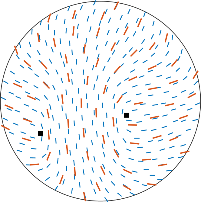
(a) $f\colon\mathbb{S}^{2}\to\mathbb{R}P^{2}$

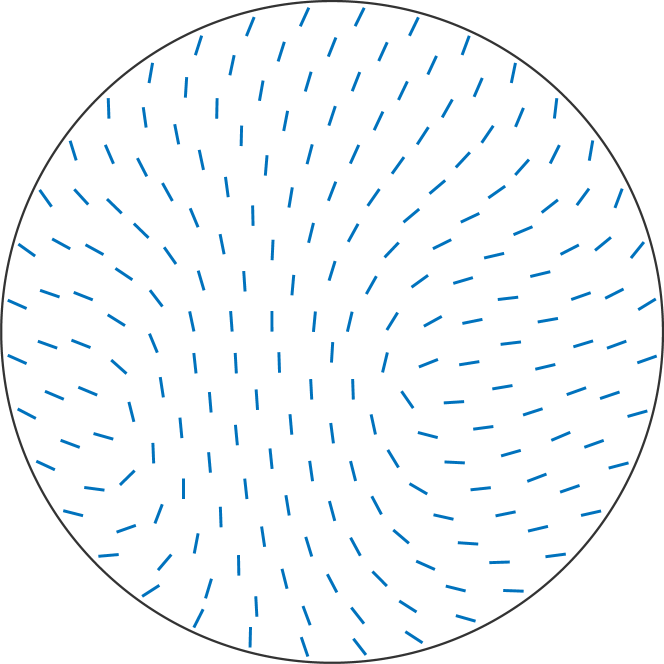
(b) $P_{\mathbb{R}P^{2}}\circ S_{8}(\mathcal{E}\circ f)$

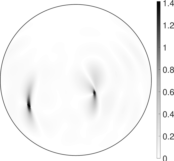
(c) $\left\lVert\smash{f-P_{\mathbb{R}P^{2}}\circ S_{8}(\mathcal{E}\circ f)}\right\rVert_{2}$.

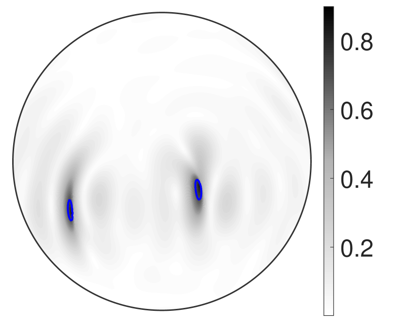
(d) $\left\lVert\smash{f-S_{8}(\mathcal{E}\circ f)}\right\rVert_{2}$.

Figure 1: Polarization directions of the fastest shear wave with respect to the propagation direction $\mathbf{\boldsymbol{x}}\in\mathbb{S}^{2}$ plotted as vector fields on the upper hemisphere. The left upper image (a) displays the true polarization directions $f(\mathbf{\boldsymbol{x}})\in\mathbb{R}P^{2}$. The right upper image (b) is the harmonic approximation $P_{\mathbb{R}P^{2}}\circ S_{8}(\mathcal{E}\circ f)(\mathbf{\boldsymbol{x}})$ using the sampling points marked red in (a). The lower left image (c) displays the norm of the point-wise residual. The lower right image (d) displays the error of the linear approximation, i.e. exactly half of the upper bound from Theorem 3.1. We marked red the regions where this residual is bigger than the reach of the manifold.

We determined the derivatives of $f$ numerically by choosing a basis ${\mathbf{\boldsymbol{t}}_{1},\mathbf{\boldsymbol{t}}_{2}}$ in the tangent space $T_{\mathbf{\boldsymbol{x}}}\mathbb{S}^{2}$ and approximating the columns $\mathbf{\boldsymbol{v}}_{i}\in\mathbb{R}^{9}$, $i=1,2$ of $\,\mathrm{d}f(\mathbf{\boldsymbol{x}})\in\mathbb{R}^{9\times 2}$ by the difference quotients

$$\mathbf{\boldsymbol{v}}_{i}=\frac{1}{h}\left(f\bigl{(}\tfrac{\mathbf{\boldsymbol{x}}+h\,\mathbf{\boldsymbol{t}}_{i}}{\left\lVert\smash{\mathbf{\boldsymbol{x}}+h\,\mathbf{\boldsymbol{t}}_{i}}\right\rVert_{2}}\bigr{)}-f(\mathbf{\boldsymbol{x}})\right),$$

with $h=10^{-6}$. The norm of the derivative is depicted in Fig. 2(a) and clearly shows the position of the singularities. In Fig. 2(b) the error between $\mathrm{d}f(\mathbf{\boldsymbol{x}})$ and the differential of harmonic approximation $\,\mathrm{d}(P_{\mathbb{R}P^{2}}\circ S_{64})(\mathcal{E}\circ f)(\mathbf{\boldsymbol{x}})$ is plotted as a function of the propagation direction $\mathbf{\boldsymbol{x}}\in\mathbb{S}^{2}$. Since the differential $\mathrm{d}f(\mathbf{\boldsymbol{x}})$ is a matrix in $\mathbb{R}^{9\times 2}$, we consider here the spectral norm of the error matrix. In order to illustrate our theoretical result of Theorem 3.2 we plotted our theoretical upper bound on that approximation error of the derivative in Fig. 2(c). It should be noted that for the differential we needed to increased the polynomial degree to $L=64$ with $21000$ sample points in order to obtain a reasonable approximation at some distance to the singularities.

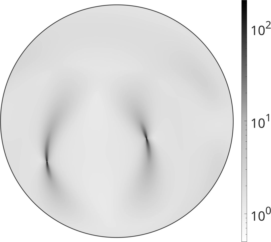
(a) $\left\lVert\smash{df(x)}\right\rVert_{2}$

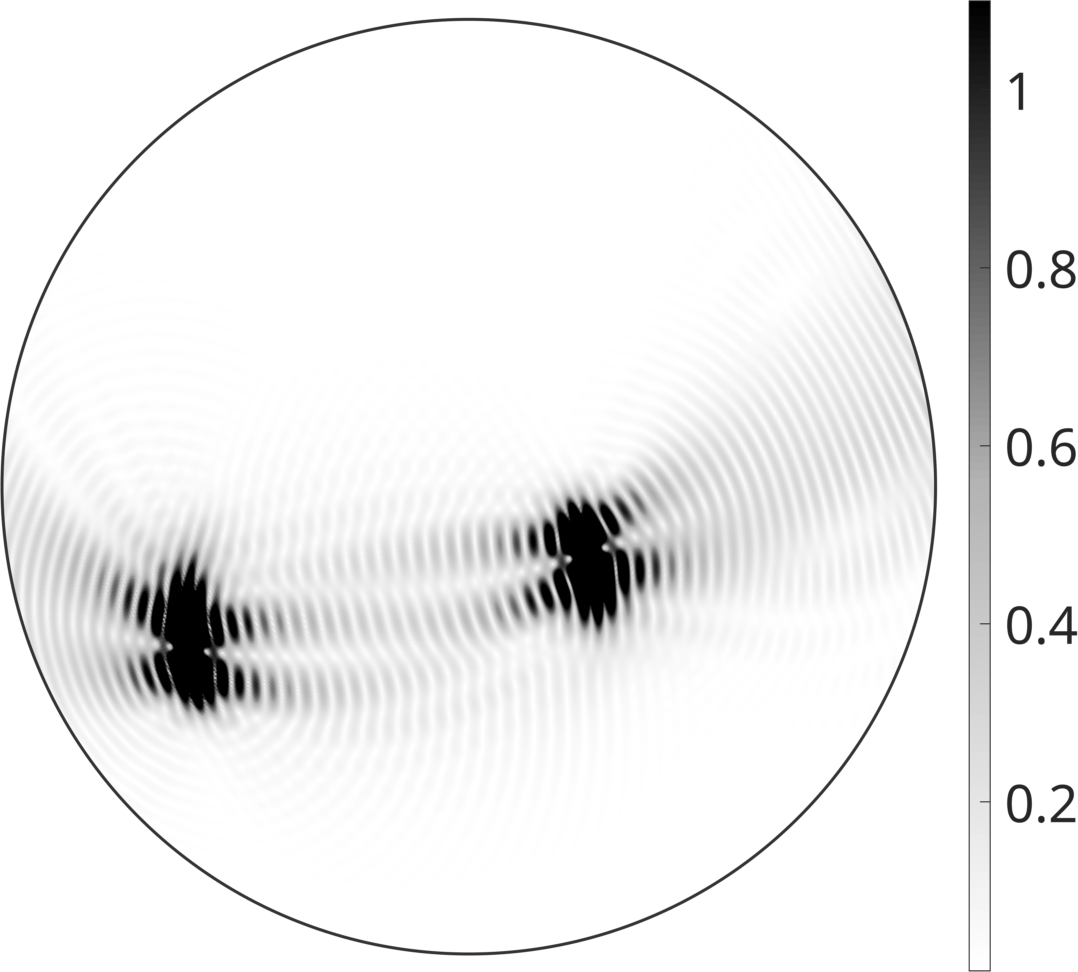
(b) $\left\lVert\smash{df(x)-dP_{\mathbb{R}P^{2}}\circ\tilde{f}}\right\rVert_{2}$

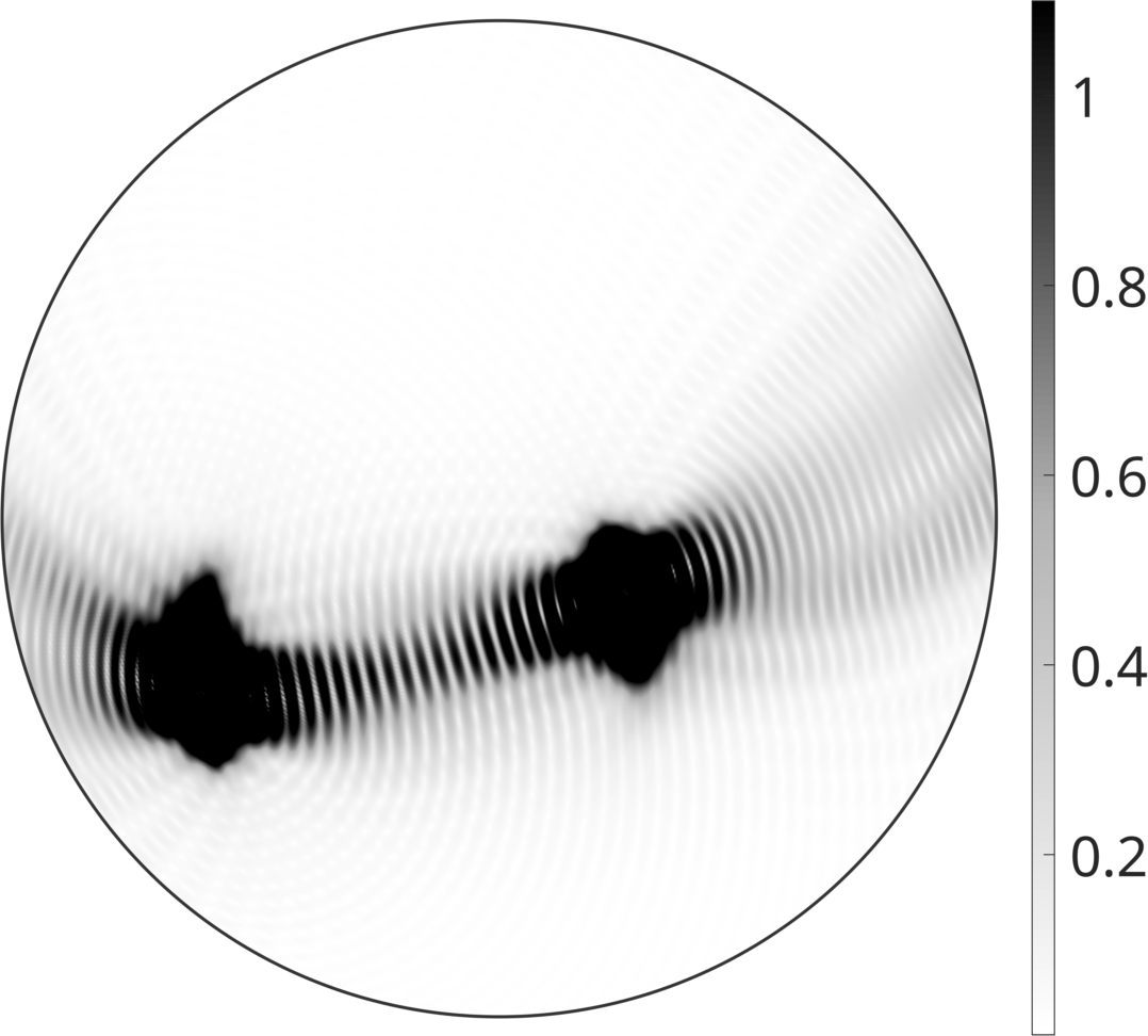
(c) Bound from Thm. 3.2.

Figure 2: The left image (a) shows the point-wise norm of the differential $\,\mathrm{d}f$. The middle image (b) depicts the approximation error between the differential of the original function $f$ and the differential of its harmonic approximation $P_{\mathbb{R}P^{2}}\circ\tilde{f}=P_{\mathbb{R}P^{2}}\circ S_{64}(\mathcal{E}\circ f)$. The right images (c) gives the upper bound for (b) from Theorem 3.2.

4.2 Electron Back Scatter Diffraction

The subject of crystallographic texture analysis is the microstructure of polycrystalline materials. Locally the microstructure is described by the orientation of the atom lattice with respect to some specimen fixed reference frame. More specifically, one describes the local orientation of the atom lattice by a coset $[\mathbf{\boldsymbol{R}}]_{\mathcal{S}}\in\mathrm{SO}(3)/\mathcal{S}$ of the rotation group $\mathrm{SO}(3)$ modulo the finite subgroup $\mathcal{S}\subset\mathrm{SO}(3)$, called point group. The point group of a crystal consists of all symmetries of its atom lattice and is either one of the cyclic groups $C_{1}$, $C_{2}$, $C_{3}$, $C_{4}$, $C_{6}$, the dihedral groups $D_{2}$, $D_{3}$, $D_{4}$, $D_{6}$, the tetragonal group $T$ or the octahedral group $O$. Assuming a monophase material, i.e., a material consisting only of a single type of crystals, the variation of the local orientation of the atom lattice at the surface $\Omega\subset\mathbb{R}^{2}$ of the specimen is modeled by the map

$$f\colon\Omega\to\mathrm{SO}(3)/\mathcal{S}.$$

The gradient of the function $f$, also called lattice curvature tensor $\mathbf{\boldsymbol{\kappa}}(\mathbf{\boldsymbol{x}})$, is closely related to elastic and plastic deformations the specimen has been exposed to. More specifically, it is related via the Nye equation to the dislocation density tensor $\mathbf{\boldsymbol{\alpha}}(\mathbf{\boldsymbol{x}})$, [25, 15] that describes how many lattice dislocations are geometrically necessary in order to preserve the compatibility of the lattice for a given deformation. Hence, estimating $f$ and its derivatives from experimental data is a central problem in material science.

Electron back scatter diffraction (EBSD) is an experimental technique [2, 16] for determining the local lattice orientations $f(\mathbf{\boldsymbol{x}}_{\ell})\in\mathrm{SO}(3)/\mathcal{S}$ at discrete sampling points $\mathbf{\boldsymbol{x}}_{i,j}\in\Omega$. An example of such EBSD data is the $\mathrm{SO}(3)/\mathcal{S}$ - valued image displayed in Fig. 3. It describes the variation of lattice orientation at the surface of an Aluminum alloy of size $200\mu m\times 150\mu m$ at an resolution of $0.4\mu m$. The symmetry group in this case is the octahedral group $O$.

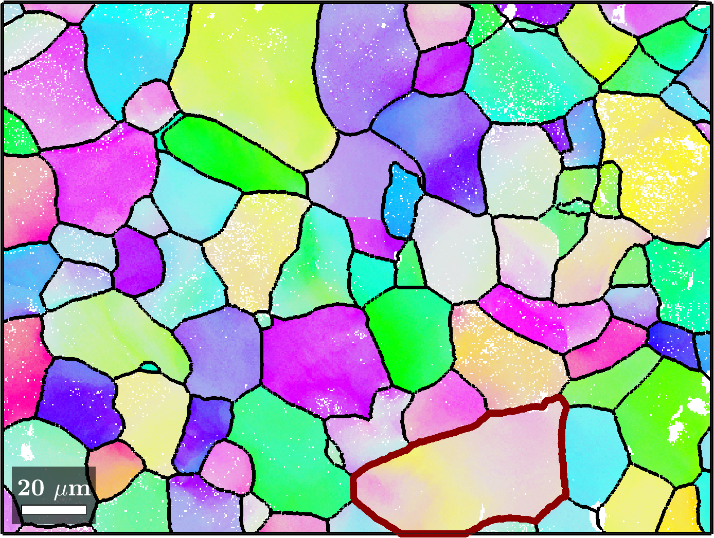
(a) full map with a global color key

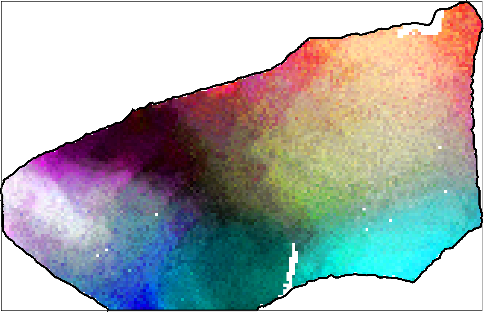
(b) single grain with a local color key

Figure 3: The raw EBSD data. Each of the $410$ x $547$ pixels corresponds to a single orientation measurement at the surface of the specimen. The color is computed by the procedure described in [23]. The $5\%$ white pixels in Fig. (a) correspond to corrupted measurements with no data. The data has been segmented into $92$ grains as outlined by the black boundaries.

The data is displayed with respect to two different color keys. In Fig. 3(a) the colors are assigned globally to the cosets $f(\mathbf{\boldsymbol{x}})\in\mathrm{SO}(3)/O$ as described in [23]. Regions of similar lattice orientation form so-called grains as outlined by the black boundaries. In Fig. 3(b) only the single grain outlined by the red boundary in Fig. 3(a) is displayed. For this grain we computed an average lattice orientation $[\mathbf{\boldsymbol{M}}]\in\mathrm{SO}(3)/O$ and selected for each coset $f(\mathbf{\boldsymbol{x}})\in\mathrm{SO}(3)/O$ the rotation $\mathbf{\boldsymbol{R}}(x)\in[\mathbf{\boldsymbol{M}}^{-1}f(\mathbf{\boldsymbol{x}})]$ with the smallest rotational angle. Next we associated a color to $\mathbf{\boldsymbol{R}}(x)$ according to a spherical color representation where the rotational angle of $\mathbf{\boldsymbol{R}}(x)$ determines the saturation and the rotational axis hue and value. More details on this orientation coloring can be found in [31].

Estimating the derivative from such a noisy map of lattice orientations is usually not a good idea as we will see later. Reducing the noise by means of local approximation methods has been discussed in [14, 28]. In order to demonstrate our embedding based approximation approach we make use of the locally isometric embedding $\mathcal{E}_{O}\colon\mathrm{SO}(3)/O\to\mathbb{R}^{9}$ described in [13] and proceed as follows

1. Compute an $\mathbb{R}^{9}$-valued image $\mathbf{\boldsymbol{u}}_{i,j}=\mathcal{E}_{O}(f(\mathbf{\boldsymbol{x}}_{i,j}))$.

2. Approximate the $\mathbb{R}^{9}$-valued image using a cosine series $\tilde{u}\colon\Omega\to\mathbb{R}^{9}$ computed by robust, penalized least squares [6].

3. Evaluate the function $\tilde{u}$ at the grid points $\mathbf{\boldsymbol{x}}_{i,j}$ to obtain a noise reduced $\mathbb{R}^{9}$-valued image $\tilde{\mathbf{\boldsymbol{u}}}_{i,j}$.

4. Compute the projection of $\mathbf{\boldsymbol{\tilde{u}}}_{i,j}$ onto the embedding $\mathcal{E}_{O}(\mathrm{SO}(3)/O)$ of the quotient and apply the inverse map $\mathcal{E}_{O}^{-1}$ to end up with a noise reduced $\mathrm{SO}(3)/O$-valued image $\tilde{f}(\mathbf{\boldsymbol{x}}_{i,j})$.

The resulting image is depicted in Figure 4. We observe that all no data pixels have been inpainted and that the magnified part 4(b) is much less noisy in comparison to Fig. 3(b).

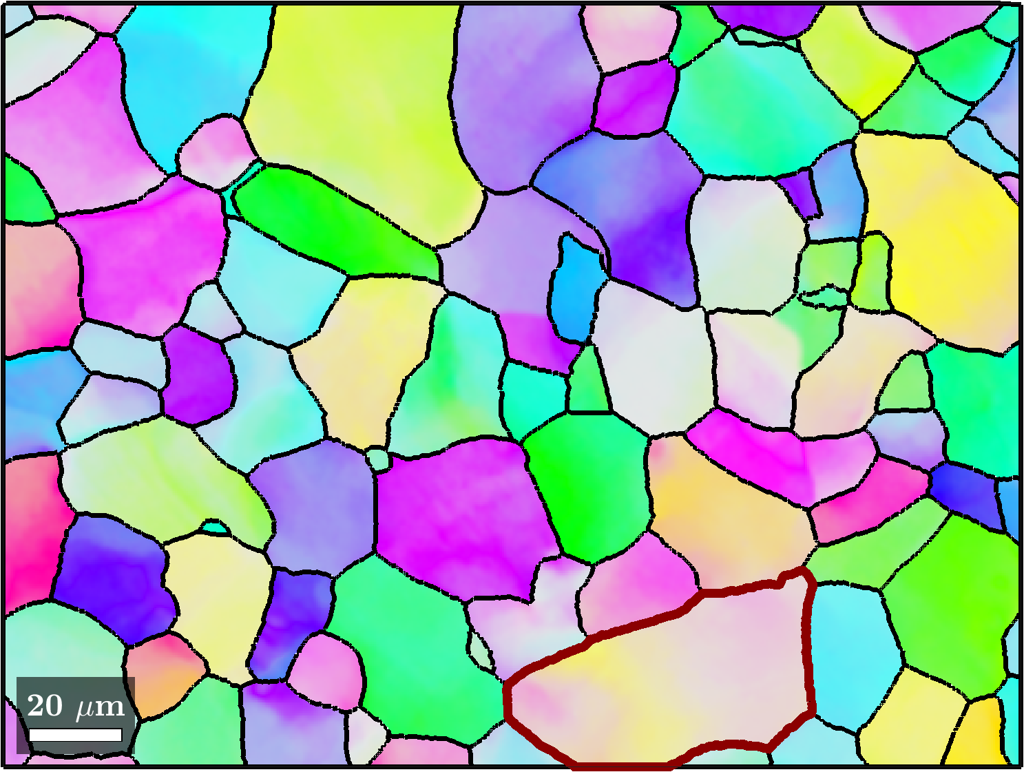
(a) full map of the approximated data

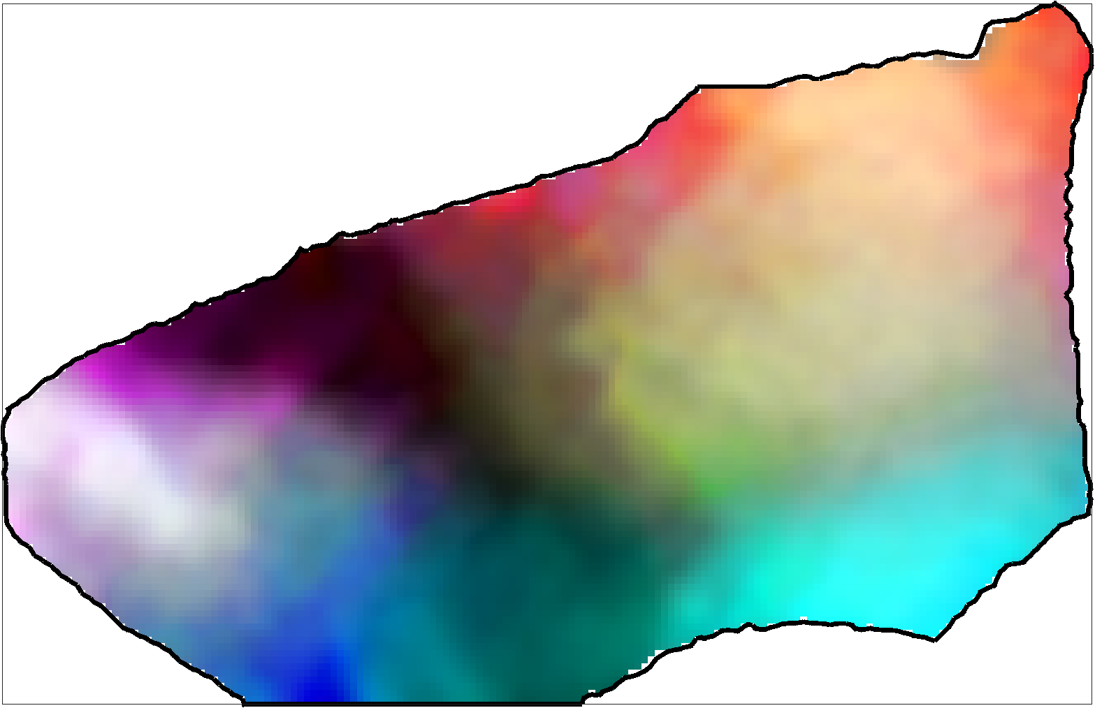
(b) single grain with a local color key

Figure 4: EBSD map from Fig. 3 after the embedding based approximation approach.

For the computation of the lattice curvature tensor $\mathbf{\boldsymbol{\kappa}}$ we use the skew symmetric matrices

$$\mathbf{\boldsymbol{s}}^{(1)}=\begin{pmatrix}0&0&0\\ 0&0&-1\\ 0&1&0\end{pmatrix},\quad\mathbf{\boldsymbol{s}}^{(2)}=\begin{pmatrix}0&0&-1\\ 0&0&0\\ 1&0&0\end{pmatrix},\quad\mathbf{\boldsymbol{s}}^{(3)}=\begin{pmatrix}0&-1&0\\ 1&0&0\\ 0&0&0\end{pmatrix},$$

to fix the basis $\mathbf{\boldsymbol{R}}\mathbf{\boldsymbol{s}}^{(1)},\mathbf{\boldsymbol{R}}\mathbf{\boldsymbol{s}}^{(2)},\mathbf{\boldsymbol{R}}\mathbf{\boldsymbol{s}}^{(3)}$ in the tangential space $T_{\mathbf{\boldsymbol{R}}}\mathrm{SO}(3)/O$ at some rotation $\mathbf{\boldsymbol{R}}\in\mathrm{SO}(3)$. With respect to this basis the differential $D\mathcal{E}(\mathbf{\boldsymbol{R}})\colon T_{\mathbf{\boldsymbol{R}}}\mathrm{SO}(3)/O\to\mathbb{R}^{9}$ of the embedding $\mathcal{E}\colon\mathrm{SO}(3)/O\to\mathbb{R}^{9}$ can be represented as a full rank $3\times 9$ matrix. Furthermore, we obtain for the differential $D\tilde{u}\colon\mathbb{R}^{2}\to\mathbb{R}^{9}$ of the embedded image $\tilde{u}=\mathcal{E}\circ\tilde{f}\colon\Omega\to\mathbb{R}^{9}$ at some point $\mathbf{\boldsymbol{x}}\in\Omega$ the matrix product $D\tilde{u}(\mathbf{\boldsymbol{x}})=D\mathcal{E}(\tilde{f}(\mathbf{\boldsymbol{x}}))Df(\mathbf{\boldsymbol{x}})$. Hence, the lattice curvature tensor $\tilde{\mathbf{\boldsymbol{\kappa}}}$ of the noise reduced EBSD map evaluates to

$$\tilde{\mathbf{\boldsymbol{\kappa}}}(\mathbf{\boldsymbol{x}})=D\tilde{f}(\mathbf{\boldsymbol{x}})=\left(D\mathcal{E}(\tilde{f}(\mathbf{\boldsymbol{x}}))D\mathcal{E}(\tilde{f}(\mathbf{\boldsymbol{x}}))^{\top}\right)^{-1}D\mathcal{E}(\tilde{u}f(\mathbf{\boldsymbol{x}}))^{\top}D\tilde{u}(\mathbf{\boldsymbol{x}}).$$

The map of the first component $\tilde{\kappa}_{1,1}$ of the lattice curvature tensor obtained from the approximating function $\tilde{u}$ is depicted in Fig. 5(b). For comparison we plotted in Fig. 5(a) a finite difference approximation

$$\kappa(\mathbf{\boldsymbol{x}}_{i,j})_{1,1}=\frac{\log_{f(\mathbf{\boldsymbol{x}}_{i,j})}(f(\mathbf{\boldsymbol{x}}_{i+1,j}))}{[x_{i+1,j}-x_{i,j}]_{1}},$$

derived from the discrete data $f(\mathbf{\boldsymbol{x}}_{i,j})$. Here, we denoted by $\log_{\mathbf{\boldsymbol{R}}}\colon\mathrm{SO}(3)/O\to T_{\mathbf{\boldsymbol{R}}}\mathrm{SO}(3)/O$ the logarithmic mapping with respect to the base point $\mathbf{\boldsymbol{R}}\in\mathrm{SO}(3)/O$. As expected, we observe that the lattice curvature tensor $\tilde{\kappa}$ derived from the approximated map $\tilde{u}$ is much less noisy.

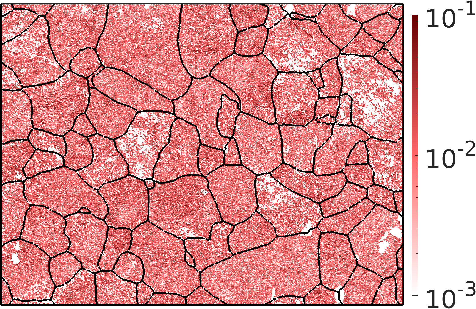
(a) $\kappa_{1,1}$ of noisy map.

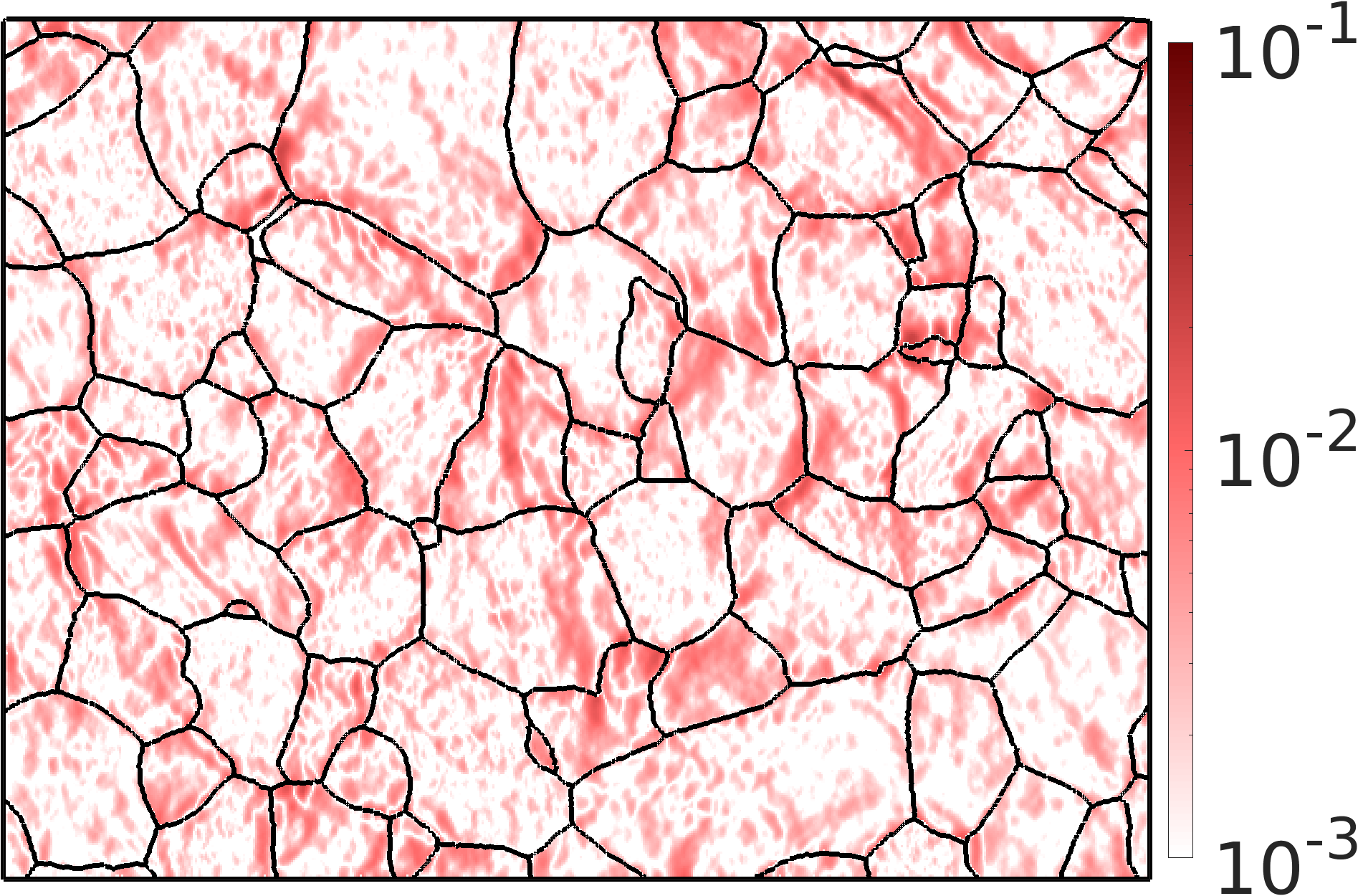
(b) $\kappa_{1,1}$ of noise reduced map.

Figure 5: First coefficient $\tilde{\kappa}_{1,1}(\mathbf{\boldsymbol{x}})$ of the lattice curvature tensor of the $SO(3)/O$-valued map depicted in Fig. 3 (left) and Fig. 4 (right).

Conclusion and further directions

We proposed a method for approximating a manifold-valued function using an embedding approach and a generic approximation operator $I_{\mathbb{R}^{d}}$ into the Euclidean space. Our main result are the Theorems 3.1 and 3.2 which give upper bounds on the approximation error for the function values as well as for the derivatives. The central requirement of the Theorems is that generic approximation $I_{\mathbb{R}^{d}}f(\mathbf{\boldsymbol{x}})$ has distance less than $\tau$ to the manifold $\mathcal{M}$. For the approximation error of the function values it is only important that $I_{\mathbb{R}^{d}}f(\mathbf{\boldsymbol{x}})$ is within the reach of the manifold $\mathcal{M}$ and has no impact on the convergence rate or the constants. However, for the approximation error of the derivatives the constant of the upper bound becomes arbitrary large for $I_{\mathbb{R}^{d}}f(\mathbf{\boldsymbol{x}})$ close to the reach. This stresses the importance of finding embeddings with a large reach.

The basis of our approximation approach is to find a suitable embedding of the manifold $\mathcal{M}$ into $\mathbb{R}^{d}$. For an arbitrary manifold this can be a difficult challenge. However, for many important manifolds low dimensional embeddings are well known. A further challenge is the numerical realization of the projection operator $P_{\mathcal{M}}$ on the manifold needed for our embedding based approximation method. This leads to a problem of manifold optimization.

So far we did not deal with noisy data. The main challenge here is to guaranty that $I_{\mathbb{R}^{d}}f(\mathbf{\boldsymbol{x}})$ is sufficiently close to the manifold even for noisy data. Up to this point it is not clear how strongly noise that keeps the data on the manifold can increase the distance of $I_{\mathbb{R}^{d}}f(\mathbf{\boldsymbol{x}})$ to the manifold.

Appendix A Bound for the commutator

To bound the term $\left\lVert\smash{\,\mathrm{d}P_{\mathcal{M}}(\mathbf{\boldsymbol{m}})-\,\mathrm{d}P_{\mathcal{M}}(\mathbf{\boldsymbol{z}})}\right\rVert_{2}$ in section 2.4 we need a lemma, which is based on linear algebra.

Lemma A.1.

Let $\mathbf{\boldsymbol{T}}$ be a projection matrix and $\mathbf{\boldsymbol{R}}$ be a rotation matrix. Then there holds for the commutator

$$\left\lVert\smash{\mathbf{\boldsymbol{T}}\mathbf{\boldsymbol{R}}-\mathbf{\boldsymbol{R}}\mathbf{\boldsymbol{T}}}\right\rVert_{2}\leq\left\lVert\smash{\mathbf{\boldsymbol{I}}-\mathbf{\boldsymbol{R}}}\right\rVert_{2},$$

where again $\left\lVert\smash{\cdot}\right\rVert_{2}$ denotes the spectral norm.

Proof.

Since the spectral norm doesn’t change under change of basis, we choose a matrix representation where the projection matrix has the form

$$\mathbf{\boldsymbol{T}}=\begin{pmatrix}\mathbf{\boldsymbol{I}}&\mathbf{\boldsymbol{0}}\\ \mathbf{\boldsymbol{0}}&\mathbf{\boldsymbol{0}}\end{pmatrix},$$

where $\mathbf{\boldsymbol{I}}$ is the identity matrix of dimension $D$. Then we also write the rotation matrix $\mathbf{\boldsymbol{R}}$ in these blocks:

$$\mathbf{\boldsymbol{R}}=\begin{pmatrix}\mathbf{\boldsymbol{R}}_{11}&\mathbf{\boldsymbol{R}}_{12}\\ \mathbf{\boldsymbol{R}}_{21}&\mathbf{\boldsymbol{R}}_{22}\end{pmatrix}.$$

Simple matrix multiplication yields because of the orthogonality of $\mathbf{\boldsymbol{R}}$

$$(\mathbf{\boldsymbol{T}}\mathbf{\boldsymbol{R}}-\mathbf{\boldsymbol{R}}\mathbf{\boldsymbol{T}})^{\top}(\mathbf{\boldsymbol{T}}\mathbf{\boldsymbol{R}}-\mathbf{\boldsymbol{R}}\mathbf{\boldsymbol{T}}) =\mathbf{\boldsymbol{R}}^{\top}\mathbf{\boldsymbol{T}}\mathbf{\boldsymbol{R}}-\mathbf{\boldsymbol{R}}^{\top}\mathbf{\boldsymbol{T}}\mathbf{\boldsymbol{R}}\mathbf{\boldsymbol{T}}-\mathbf{\boldsymbol{T}}\mathbf{\boldsymbol{R}}^{\top}\mathbf{\boldsymbol{T}}\mathbf{\boldsymbol{R}}+\mathbf{\boldsymbol{T}}$$

$$=\begin{pmatrix}\mathbf{\boldsymbol{I}}-\mathbf{\boldsymbol{R}}_{11}^{\top}\mathbf{\boldsymbol{R}}_{11}&\mathbf{\boldsymbol{0}}\\ \mathbf{\boldsymbol{0}}&\mathbf{\boldsymbol{R}}_{12}^{\top}\mathbf{\boldsymbol{R}}_{12}\end{pmatrix}$$

$$=\begin{pmatrix}\mathbf{\boldsymbol{R}}_{21}^{\top}\mathbf{\boldsymbol{R}}_{21}&\mathbf{\boldsymbol{0}}\\ \mathbf{\boldsymbol{0}}&\mathbf{\boldsymbol{R}}_{12}^{\top}\mathbf{\boldsymbol{R}}_{12}\end{pmatrix}$$

On the other hand there holds, again with help of the orthogonality of $\mathbf{\boldsymbol{R}}$,

$$(\mathbf{\boldsymbol{I}}-\mathbf{\boldsymbol{R}})^{\top}(\mathbf{\boldsymbol{I}}-\mathbf{\boldsymbol{R}}) =2\mathbf{\boldsymbol{I}}-\mathbf{\boldsymbol{R}}-\mathbf{\boldsymbol{R}}^{\top}=\begin{pmatrix}2\mathbf{\boldsymbol{I}}-\mathbf{\boldsymbol{R}}_{11}-\mathbf{\boldsymbol{R}}_{11}^{\top}&-\mathbf{\boldsymbol{R}}_{12}-\mathbf{\boldsymbol{R}}_{21}^{\top}\\ -\mathbf{\boldsymbol{R}}_{21}-\mathbf{\boldsymbol{R}}_{12}^{\top}&2\mathbf{\boldsymbol{I}}-\mathbf{\boldsymbol{R}}_{22}-\mathbf{\boldsymbol{R}}_{22}^{\top}\end{pmatrix}$$

$$=\begin{pmatrix}(\mathbf{\boldsymbol{I}}-\mathbf{\boldsymbol{R}}_{11}^{\top})(\mathbf{\boldsymbol{I}}-\mathbf{\boldsymbol{R}}_{11})+\mathbf{\boldsymbol{I}}-\mathbf{\boldsymbol{R}}_{11}^{\top}\mathbf{\boldsymbol{R}}_{11}&-\mathbf{\boldsymbol{R}}_{12}-\mathbf{\boldsymbol{R}}_{21}^{\top}\\ -\mathbf{\boldsymbol{R}}_{21}-\mathbf{\boldsymbol{R}}_{12}^{\top}&(\mathbf{\boldsymbol{I}}-\mathbf{\boldsymbol{R}}_{22}^{\top})(\mathbf{\boldsymbol{I}}-\mathbf{\boldsymbol{R}}_{22})+\mathbf{\boldsymbol{I}}-\mathbf{\boldsymbol{R}}_{22}^{\top}\mathbf{\boldsymbol{R}}_{22}\end{pmatrix}$$

$$=\begin{pmatrix}(\mathbf{\boldsymbol{I}}-\mathbf{\boldsymbol{R}}_{11}^{\top})(\mathbf{\boldsymbol{I}}-\mathbf{\boldsymbol{R}}_{11})+\mathbf{\boldsymbol{R}}_{21}^{\top}\mathbf{\boldsymbol{R}}_{21}&-\mathbf{\boldsymbol{R}}_{12}-\mathbf{\boldsymbol{R}}_{21}^{\top}\\ -\mathbf{\boldsymbol{R}}_{21}-\mathbf{\boldsymbol{R}}_{12}^{\top}&(\mathbf{\boldsymbol{I}}-\mathbf{\boldsymbol{R}}_{22}^{\top})(\mathbf{\boldsymbol{I}}-\mathbf{\boldsymbol{R}}_{22})+\mathbf{\boldsymbol{R}}_{12}^{\top}\mathbf{\boldsymbol{R}}_{12}\end{pmatrix}.$$

The spectral norm of a matrix $\mathbf{\boldsymbol{A}}$, i.e., the largest absolute value of the eigenvalues can be written as

$$\left\lVert\smash{\mathbf{\boldsymbol{A}}}\right\rVert_{2}^{2}=\max_{\left\lVert\smash{\mathbf{\boldsymbol{x}}}\right\rVert_{2}=1}\left\lVert\smash{\mathbf{\boldsymbol{x}}^{\top}\mathbf{\boldsymbol{A}}^{\top}\mathbf{\boldsymbol{A}}\mathbf{\boldsymbol{x}}}\right\rVert_{2}.$$

For that reason we choose the vector $\mathbf{\boldsymbol{x}}$ as the eigenvector of the matrix $(\mathbf{\boldsymbol{T}}\mathbf{\boldsymbol{R}}-\mathbf{\boldsymbol{R}}\mathbf{\boldsymbol{T}})^{\top}(\mathbf{\boldsymbol{T}}\mathbf{\boldsymbol{R}}-\mathbf{\boldsymbol{R}}\mathbf{\boldsymbol{T}})$. Since the eigenvalues and eigenvectors of a block-diagonal matrix are the union of the eigenvalues and eigenvectors, i.e., there holds $\mathbf{\boldsymbol{x}}=\begin{pmatrix}\mathbf{\boldsymbol{x}}_{1}&\mathbf{\boldsymbol{0}}\end{pmatrix}^{\top}$ or $\mathbf{\boldsymbol{x}}=\begin{pmatrix}\mathbf{\boldsymbol{0}}&\mathbf{\boldsymbol{x}}_{2}\end{pmatrix}^{\top}$. We assume the first case, the other one is analog. Hence, there holds

$$\left\lVert\smash{\mathbf{\boldsymbol{T}}\mathbf{\boldsymbol{R}}-\mathbf{\boldsymbol{R}}\mathbf{\boldsymbol{T}}}\right\rVert_{2}^{2}=\mathbf{\boldsymbol{x}}^{\top}\begin{pmatrix}\mathbf{\boldsymbol{R}}_{21}^{\top}\mathbf{\boldsymbol{R}}_{21}&\mathbf{\boldsymbol{0}}\\ \mathbf{\boldsymbol{0}}&\mathbf{\boldsymbol{R}}_{12}^{\top}\mathbf{\boldsymbol{R}}_{12}\end{pmatrix}\mathbf{\boldsymbol{x}}=\mathbf{\boldsymbol{x}}_{1}^{\top}\mathbf{\boldsymbol{R}}_{21}^{\top}\mathbf{\boldsymbol{R}}_{21}\mathbf{\boldsymbol{x}}_{1}.$$

If we look at the norm of the matrix $\mathbf{\boldsymbol{I}}-\mathbf{\boldsymbol{R}}$, we get

$$\left\lVert\smash{\mathbf{\boldsymbol{I}}-\mathbf{\boldsymbol{R}}}\right\rVert_{2}^{2} \geq\mathbf{\boldsymbol{x}}^{\top}\,(\mathbf{\boldsymbol{I}}-\mathbf{\boldsymbol{R}})^{\top}(\mathbf{\boldsymbol{I}}-\mathbf{\boldsymbol{R}})\,\mathbf{\boldsymbol{x}}=\mathbf{\boldsymbol{x}}_{1}^{\top}\,\left((\mathbf{\boldsymbol{I}}-\mathbf{\boldsymbol{R}}_{11}^{\top})(\mathbf{\boldsymbol{I}}-\mathbf{\boldsymbol{R}}_{11})+\mathbf{\boldsymbol{R}}_{21}^{\top}\mathbf{\boldsymbol{R}}_{21}\right)\,\mathbf{\boldsymbol{x}}_{1}$$

$$\geq\mathbf{\boldsymbol{x}}_{1}^{\top}\mathbf{\boldsymbol{R}}_{21}^{\top}\mathbf{\boldsymbol{R}}_{21}\mathbf{\boldsymbol{x}}_{1},$$

since the eigenvalues of $(\mathbf{\boldsymbol{I}}-\mathbf{\boldsymbol{R}}_{11}^{\top})(\mathbf{\boldsymbol{I}}-\mathbf{\boldsymbol{R}}_{11})$ are positive. Putting this together and taking the square root, yields the assertion. ∎

References

- [1] E. Aamari, J. Kim, F. Chazal, B. Michel, A. Rinaldo, and L. Wasserman. Estimating the reach of a manifold. Electron. J. Statist., 13(1):1359–1399, 2019.
- [2] B. L. Adams, S. I. Wright, and K. Kunze. Orientation imaging: The emergence of a new microscopy. Metall. Mater. Trans. A, 24:819–831, 1993.
- [3] J.-D. Boissonnat, A. Lieutier, and M. Wintraecken. The reach, metric distortion, geodesic convexity and the variation of tangent spaces. J. Appl. Comput. Topol., 3:1–30, 07 2019.
- [4] A. Constantin. Fourier Analysis: Volume 1, Theory, volume 85. Cambridge University Press, 2016.
- [5] D.Mainprice, R. Hielscher, and H. Schaeben. Calculating anisotropic physical properties from texture data using the MTEX open source package. Geological Society, London, Special Publications, 360:175–192, 2011.
- [6] D. Garcia. Robust smoothing of gridded data in one and higher dimensions with missing values. Comput. Statist. Data Anal., 54(4):1167–1178, 2010.
- [7] E. S. Gawlik and M. Leok. Embedding-based interpolation on the special orthogonal group. SIAM J. Sci. Comput., 40(2):A721–A746, 2018.
-
[8]
M. Gräf.
Quadrature rules on manifolds.
http://homepage.univie.ac.at/manuel.graef/quadrature.php, 2013. - [9] P. Grohs. Smoothness of interpolatory multivariate subdivision in lie groups. IMA J. Numer. Anal., 29(3):760–772, 2009.
- [10] P. Grohs. Approximation order from stability for nonlinear subdivision schemes. J. Approx. Theory, 162(5):1085–1094, 2010.
- [11] P. Grohs and M. Sprecher. Projection-based quasiinterpolation in manifolds. 2013. Technical Report 2013-23, Seminar for Applied Mathematics, ETH Zürich, Switzerland.
- [12] P. Grohs, M. Sprecher, and T. Yu. Scattered manifold-valued data approximation. Numer. Math., 135:987–1010, 2017.
- [13] R. Hielscher and L. Lippert. Locally isometric embeddings of quotients of the rotation group modulo finite symmetries. J. Multivar. Anal., 185:104764, 2021.
- [14] R. Hielscher, C. Silbermann, E. Schmiedl, and J. Ihlemann. Denoising of crystal orientation maps. J. Appl. Cryst., 52, 2019.
- [15] P. Konijnenberg, S. Zaefferer, and D. Raabe. Assessment of geometrically necessary dislocation levels derived by 3d ebsd. Acta Materialia, 99:402 – 414, 2015.
- [16] K. Kunze, S. I. Wright, B. L. Adams, and D. J. Dingley. Advances in automatic EBSP single orientation measurements. Textures and Microstructures, 20:41–54, 1993.
- [17] J. Lee. Introduction to Smooth Manifolds. Springer-Verlag New York, second edition, 2012.
- [18] D. Mainprice. Seismic Anisotropy of the Deep Earth from a Mineral and Rock Physics Perspective. In Treatese of Geophysics, vol. 2, pages 437–491. Elsevier, 2007.
- [19] V. Michel. Lectures on Constructive Approximation: Fourier, Spline, and Wavelet Methods on the Real Line, the Sphere, and the Ball. Birkhäuser, New York, 2013.
- [20] M. Moakher. Means and averaging in the group of rotations. SIAM J. Matrix Anal. Appl, 24, 04 2002.
- [21] J. Nash. C1 isometric imbeddings. Ann. Math., 60(3):383–396, 1954.
- [22] P. Niyogi, S. Smale, and S. Weinberger. Finding the Homology of Submanifolds with High Confidence from Random Samples. Discrete Comput. Geom., 39:419–441, 03 2008.
- [23] G. Nolze and R. Hielscher. Orientations – perfectly colored. J. Appl. Cryst., 49:1786–1802, 2016.
- [24] J. F. Nye. Physical Properties of Crystals: Their Representation by Tensors 852 and Matrices. Oxford Univ. Press, England, 2nd ed. edition, 1985.
- [25] W. Pantleon. Resolving the geometrically necessary dislocation content by conventional electron backscattering diffraction. Scripta Materialia, 58:994–997, 2008.
- [26] G. Plonka, D. Potts, G. Steidl, and M. Tasche. Numerical Fourier Analysis. Applied and Numerical Harmonic Analysis. Birkhäuser, 2018.
- [27] A. Sarlette and R. Sepulchre. Consensus optimization on manifolds, 2008.
- [28] A. Seret, C. Moussa, M. Bernacki, J. Signorelli, and N. Bozzolo. Estimation of geometrically necessary dislocation density from filtered EBSD data by a local linear adaptation of smoothing splines. J. Appl. Crystallogr., 52(3):548–563, Jun 2019.
- [29] N. Sharon and U. Itai. Approximation schemes for functions of positive-definite matrix values. IMA J. Numer. Anal., 33(4):1436–1468, 04 2013.
- [30] T. Shingel. Interpolation in special orthogonal groups. IMA J. Numer. Anal., 29(3):731–745, 07 2008.
- [31] K. Thomsen, K. Mehnert, P. W. Trimby, and A. Gholinia. Quaternion-based disorientation coloring of orientation maps. Ultramicroscopy, 182:62–67, 2017.
- [32] J. Wallner and N. Dyn. Convergence and C1 analysis of subdivision schemes on manifolds by proximity. Comput. Aided Geom. Des., 22(7):593–622, 2005. Geometric Modelling and Differential Geometry.
- [33] G. Xie and T. P.-Y. Yu. Smoothness equivalence properties of manifold-valued data subdivision schemes based on the projection approach. SIAM J. Numer. Anal., 45:1200–1225, 2007.