Elucidating the effect of intermediate resonances in the quark interaction kernel on the time-like electromagnetic pion form factor

Abstract

An exploratory study of the time-like pion electromagnetic form factor in a Poincaré-covariant bound state formalism in the isospin symmetric limit is presented. Starting from a quark interaction kernel representing gluon-intermediated interactions for valence-type quarks, non-valence effects are included by introducing pions as explicit degrees of freedom. The two most important qualitative aspects are, in view of the presented study, the opening of the dominant $\rho$-meson decay channel and the presence of a multi-particle branch cut setting in when the two-pion threshold is crossed. Based on a recent respective computation of the quark-photon vertex, the pion electromagnetic form factor for space-like and time-like kinematics is calculated. The obtained results for its absolute value and its phase compare favorably to the available experimental data, and they are analyzed in detail by confronting them to the expectations based on an isospin-symmetric version of a vector-meson dominance model.

I Introduction

Hadronic time-like form factors will be measured in upcoming experiments to an unprecedented precision. An understanding of these quantities which are displaying pronounced structures originating from hadron resonances will contribute significantly to our knowledge on the relation between the hadrons’ substructure and the hadron spectrum. On the one hand, based on respective experimental and theoretical progress in the last decades, it is by now evident that hadron resonances can be, at least in principle, described in terms of quarks and gluons. The latter, being the QCD degrees of freedom, are considered to be complete in the sense that they allow for a computation of every hadronic observable. Changing the perspective in an attempt to understand the Strong Interaction starting from the low-energy regime, a possible way of phrasing the phenomenon of confinement in QCD is the statement that all possible hadronic degrees of freedom will form also a complete set of physical states. Therefore, the equivalence of descriptions of observables in either quark and glue or hadronic degrees of freedom is a direct consequence of confinement and unitarity. This is the gist of a chain of arguments which can be sophisticated and applied to many different phenomena involving hadrons. The related picture is known under the name “quark-hadron duality”, and its consequences have been verified on the qualitative as well as the semi-quantitative level, for a review see, e.g., Ref. Melnitchouk:2005zr . A verification of this duality is, beyond the trivial fact of the absence of coloured states, the clearest experimental signature for confinement. To appreciate the scope of such a scenario it is important to note that a perfect orthogonality of the quark-glue degrees of freedom on the one hand and hadronic states on the other hand, and thus the perfect absence of “double-counting” in any of the two “languages”, is nothing else but another way to express confinement.

Gaining insight into the interplay between formation of hadronic bound states, consisting of quarks and gluons, and the open decay channels of the respective resonance is an essential element of every study of time-like form factors in kinematic regions close to a resonance. Here, attention should be paid to the fact that the hadron whose form factor is investigated and the hadronic resonance which is apparent in the form factor are both to be described as composite objects of quarks and gluons. The same is true for the hadronic decay products in a hadronic or semi-leptonic decay of the resonance. This makes evident that an approach to calculate a time-like form factor from QCD, or from a microscopic model based on QCD degrees of freedom, faces the challenging task to treat all elements appearing in the calculation on the same footing and to a sufficient degree of sophistication if the result is intended to allow for conclusions on the dynamics underlying such a form factor.

Herein, we will report on an exploratory study of the time-like pion electromagnetic form factor using functional methods. More precisely, we will employ a combination of Bethe-Salpeter and Dyson-Schwinger equations (for recent reviews on this and related approaches see, e.g., Cloet:2013jya ; Eichmann:2016yit ; Huber:2018ned ; Sanchis-Alepuz:2017jjd ). Although such an approach is capable of allowing a first-principle calculation (see, e.g., the computation of the glueball spectrum reported in ref. Huber:2020ngt ), for the task at hand this is yet out of reach. To grasp all essential features of the pions’ time-like form factor one needs to describe at least (i) the pion as bound state of quark and antiquark thereby at the same time taking into account its special role as would-be Goldstone boson of the dynamically broken chiral symmetry of QCD, (ii) the mixing, respectively, the interference of the $\rho$-meson, being described also as a quark-antiquark bound state, with a virtual photon when this photon is in turn coupled to a quark-antiquark pair via the fully renormalized quark-photon vertex, and (iii) the dominant decay channel of the $\rho$-meson, namely, $\rho\to\pi\pi$. The study presented here is now in two aspects exploratory. First of all, the interaction between quarks and antiquarks is modelled in such a way that the essential features, as implied by QCD and phenomenology, are taken into account but that it is on the other hand still manageable in such an involved calculation. Second, in several places we will make technical simplifications, especially when the such introduced error can for good reasons assumed to be small and the reduction in the computing time needed is substantial. We thus aim here more for an understanding of how the different features of the form factor arise from the QCD degrees of freedom than for a quantitative agreement with the experimental data.

In the chosen model for the quark-antiquark interaction, besides a gluon-mediated interaction also pions will be included explicitly. The reason for this is as follows: if one were able to take into account the fully renormalized quark-gluon vertex exactly within this approach, hadronic degrees of freedom will effectively emerge and thus be included in the interaction between quarks and antiquarks, respectively, they will back-feed on the quarks’ dynamics. Due to the pions’ Goldstone boson nature, and especially due to the implied small pion mass, the pions are the most important low-energy degrees of freedom within the Strong Interaction, as, e.g., also elucidated by chiral perturbation theory. And as in order to describe the physics of decays non-valence effects need to be taken into account, it is some minimal requirement for the investigation reported here to include pions as the most important non-valence-type interaction mediator in the sub-GeV region.

The interaction model herein is also chosen in view of a possible generalisation to the study of baryon form factors, and hereby especially the nucleons’ time-like form factor. In this respect one can build on existing calculations of space-like form factors from bound state amplitudes, see, e.g., refs. Eichmann:2016yit ; Nicmorus:2010sd ; Eichmann:2011vu ; Eichmann:2011pv ; Sanchis-Alepuz:2013iia ; Sanchis-Alepuz:2017mir for some recent respective work. A thorough understanding of the proton time-like form factor at very low $Q^{2}$ is a very timely subject as the upcoming PANDA experiment possesses the unique possibility to measure the proton’s electromagnetic form factors in the so-called unphysical region through the process $\bar{p}p\to l^{+}l^{-}\pi^{0}$, $l=e,\mu$ Fischer:2021kcr . At large $Q^{2}$ the question of the onset of the convergence scale between the space-like and the time-like form factors arises.

However, also the pions’ time-like electromagnetic form factor will be studied further by upcoming experiments, among other reasons because recently the consistency of the available data sets has been questioned Ananthanarayan:2020vum . Based on the long-known fact that the $\tau$ radiative decay allows to extract the pion form factor Kim:1979hx and that a very large number of $\tau$-leptons are produced at B-meson factories further high-precision data in sub-GeV region will become available.

Besides earlier lattice QCD calculations of the pions’ space-like electromagnetic form factor Brommel:2006ww ; Frezzotti:2008dr ; Boyle:2008yd ; Aoki:2009qn ; Nguyen:2011ek ; Brandt:2013dua ; Koponen:2013boa recently calculations of the time-like pion form factor have become available Meyer:2011um ; Feng:2014gba ; Bulava:2015qjz ; Erben:2019nmx . These results typically show a good agreement with the experimental data. In those calculations, the extraction of the time-like form factor employs a parameterisation based on the vector meson dominance (VMD) picture to extract from the lattice data at discrete energies the time-like pion form factor.

The exploratory calculation presented herein is done in the isospin symmetric limit. One of the effects of isospin breaking clearly visible in the time-like pion form factor is $\rho$-$\omega$ mixing, see, e.g., the review OConnell:1995nse . To this end we will employ the VMD-based fit given in OConnell:1995nse and modify it such that an expected form of the pion form factor without this mixing effect is extracted. Furthermore, we will present a simplified but numerically quite accurate VMD parameterisation of the time-like form factor which then serves as a basis for a detailed analysis of our results. Here, the focus is more on a comparison of our results with the form expected on the basis of the VMD parameterisation than on numerical agreement.

This paper is organized as follows: In Sect. II we review some facts about the electromagnetic pion form factor, employ the VMD-based fit given in OConnell:1995nse to remove the $\rho$-$\omega$ mixing effects, and provide an expected form of the pion form factor. In Sect. III we present our approach based on Bethe-Salpeter and Dyson-Schwinger equations. Our results are presented and analyzed in Sect. IV. In Sect. V we present conclusions and an outlook. Some technical details are deferred to two appendices.

II The time-like electromagnetic pion form factor

Figure 1: Electron-positron pair annihilating to a virtual photon with time-like momentum which then decays to a pion pair.

The pion, being a composite object, does not have a point-like interaction with the electromagnetic field, and the related substructure, the pion being a pseudoscalar, is related to one form factor. Considering, for example, the scattering of an electron off a pion $\pi^{+}$ one can describe the leptonic part of the interaction quite precisely in lowest-order perturbation theory, i.e., one considers the process in which the electron emits a virtual photon, and the latter couples to the pion. Defining the form factor $F_{\pi}(s)$ via the relation

$$\langle\pi^{+}(p_{1})|j^{\mu}_{e.m.}|\pi^{+}(p_{2})\rangle=e(p_{1}+p_{2})^{\mu}F_{\pi}(q^{2})\,,$$ (1)

where $q^{\mu}=p_{1}^{\mu}-p_{2}^{\mu}$ is the virtual photon momentum, and $e$ is the elementary electric charge. The $S$-matrix element for electron-pion scattering is then proportional to the form factor,

$$i{\cal M}_{e\pi\to e\pi} = e(p_{1}+p_{2})^{\mu}F_{\pi}(q^{2})D_{\rm photon}^{\mu\nu}(q)$$ (2)

$$\qquad\left(ie\bar{u}(k_{1},s_{1})\gamma_{\nu}u(k_{2},s_{2})\right)\,,$$

where $D_{\rm photon}^{\mu\nu}(q)$ is the photon propagator, and $u(k_{i},s_{i})$ is the electron spinor, see, e.g., Sect. 8.4 of Aitchison:2003tq for more details. The kinematics of this scattering process is such that the photon momentum is space-like, and without loss of generality one can assume the form factor $F_{\pi}(s)$ to be real. Charge conservation requires that for a real photon one has $F_{\pi}(0)=1$.

Turning to the process of electron-positron annihilation into a pion pair the corresponding $S$-matrix element is again proportional to the form factor, see , e.g., Sect. 8.5 of Aitchison:2003tq ,

$$i{\cal M}_{e^{+}e^{-}\to\pi^{+}\pi^{-}} = e(p_{1}+p_{2})^{\mu}F_{\pi}(q^{2})D_{\rm photon}^{\mu\nu}(q)$$ (3)

$$\qquad\left(-ie\bar{v}(k_{1},s_{1})\gamma_{\nu}u(k_{2},s_{2})\right)\,,$$

with appropriately redefined momenta. Especially, the virtual photon momentum is now time-like, cf. Fig. 1, and one measures in such an annihilation process to a pion pair the form factor for time-like momenta. Above the two-pion production threshold, i.e., in the physical region, the corresponding cut in the amplitude (3) necessitates to treat the time-like pion form factor as a complex quantity, it fulfils the dispersion relation

$$F_{\pi}(q^{2})=1+\frac{q^{2}}{\pi}\int_{4m_{\pi}^{2}}ds\frac{{\cal I}m\,F_{\pi}(s)}{s(s-q^{2}-i\epsilon)}\,.$$ (4)

Especially, it is expected that the phase of the pion form factor varies strongly in a two-pion resonance region. Below the inelastic threshold, i.e., for $s<4m_{\pi}^{2}$, the time-like pion form factor is, via Watson’s final state theorem, related to the isovector P-wave scattering phase shift $\delta_{1,1}(s)$:

$${\cal I}m\,F_{\pi}(q^{2}) = \frac{1}{2i}\left(1-e^{-2i\delta_{1,1}(s)}\right)F_{\pi}(s+i\epsilon)$$ (5)

$$= \sin(\delta_{1,1}(s))e^{-i\delta_{1,1}(s)}F_{\pi}(s+i\epsilon)\,.$$

As depicted in Fig.  1, the pion form factor contains, for time-like as well as for space-like photon virtualities, all kind of interaction processes turning a photon into a pion pair. As strong-interaction processes dominate the corresponding amplitude, and as gluons do not couple directly to photons, one decisive element of the pion form factor is the amplitude describing how the photon couples to a quark, taking hereby all possible contributing QCD processes into account. This amplitude is exactly the full quark-photon vertex. As we will see in the following, this correlation function carries information about the virtual photon’s hadronic substructure. And as will be described in detail in the next section, the other quantities needed then for calculating the pion form factor are the fully renormalized quark propagator and the pion bound state amplitude, the latter describing how an antiquark and a quark form a pionic bound state.

While our calculation is based on QCD degrees of freedom it is capable of providing an understanding why in the resonance region a vector-meson dominance (VMD) picture provides very good results for the time-like pion form factor. In addition, it will elucidate to which extent a VMD picture might be applicable in other kinematic regions.

In the VMD picture, the hadronic contribution to the photon propagator is given by mixing with electrically neutral vector mesons. Restricting to light-quark mesons, the corresponding vector meson is the $\rho^{0}$, i.e., the uncharged member of the isotriplet of vector mesons. In a would-be isospin symmetric world this would be the only vector meson below one GeV with which a virtual photon mixes because the isosinglet $\omega$ will not mix with the photon due to $G$-parity.

In the real world, isospin symmetry is broken, and one of the many effects of isospin breaking is $\rho$-$\omega$ mixing, see, e.g., the review OConnell:1995nse . This mixing and the resulting interference of states lead to quite some pronounced structure in the time-like pion form factor around $m_{\omega}^{2}$. Indeed, it is by now well understood that the sharp dip in the experimental data stems from a combination of $\rho$-$\omega$ mixing and interference effects between the decays $\rho\rightarrow\pi\pi$ and $\omega\rightarrow\pi\pi$, the latter being isospin breaking, see, e.g., Ref. OConnell:1995nse . Moreover, it has been estimated that this combination of mixing and interference effects decreases the height of the bump of the order of up to $10\%$ (see Jegerlehner:2011ti and references therein).

As the here presented exploratory calculation is performed in the isospin limit and thus $\rho$-$\omega$ mixing is neglected we estimate its effect by comparing the VMD-based fit to the pion form factor given in ref. OConnell:1995nse with a plot of the same expression but the mixing matrix element put to zero, $\Pi_{\rho\omega}=0$, see Fig. 2. As expected the resulting curve is much smoother than the one including the $\rho$-$\omega$ interference effect. Around the $\omega$ mass the deviation of the two curves can be as large as almost ten percent, however, this effect is limited to a small interval, and the two curves are practically indistinguishable outside this small interval. Therefore we expect our calculation to reproduce all qualitative features of the curve representing the case with $\rho$-$\omega$ mixing switched off, and to be in a reasonable quantitative agreement with it.

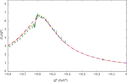
Figure 2: Absolute value of the pion form factor in the time-like ($Q^{2}<0$) domain from the VMD-based fit given in ref. OConnell:1995nse (full line) in comparison to the experimental data Ananthanarayan:2020vum . The dashed line is based on the same expression but the mixing matrix element put to zero, $\Pi_{\rho\omega}=0$.

It is instructive to analyze the momentum behaviour of a simplified version of the fit given in ref. OConnell:1995nse . In order to be in agreement with the notation in the following presentation we introduce the photon virtuality with the convention that $Q^{2}<0$ corresponds to the time-like region. In the above used fit a momentum dependent expression for the width of the $\rho$-meson is used. It displays the two-pion cut,

$$\Gamma_{\rho}(Q^{2})\propto\left(-Q^{2}-4m_{\pi}^{2}\right)^{3/2}\Theta(-Q^{2}-4m_{\pi}^{2})\,,$$ (6)

which is important for a qualitatively correct analytic structure of the pion form factor. However, especially close to the maximum of the pion form factor, the pion mass is quantitatively negligible, and for vanishing pion mass the momentum dependent width assumes for time-like $Q^{2}<0$ the relatively simple form

$$\Gamma_{\rho}(Q^{2})=\bar{\Gamma}_{\rho}|Q^{2}|/m_{\rho}^{2}\,,$$ (7)

where $\bar{\Gamma}_{\rho}=\Gamma_{\rho}(-m_{\rho}^{2})$. This then leads to the simplified but still quite accurate form for the fit

$$F_{\pi}(Q^{2}+i\epsilon) = 1-\frac{g_{\rho\pi\pi}}{g_{\rho}}\frac{Q^{2}(Q^{2}+m_{\rho}^{2})}{(Q^{2}+m_{\rho}^{2})^{2}+Q^{4}\bar{\Gamma}^{2}/m_{\rho}^{2}}$$ (8)

$$+ i\frac{g_{\rho\pi\pi}}{g_{\rho}}\frac{Q^{4}\bar{\Gamma}/m_{\rho}}{(Q^{2}+m_{\rho}^{2})^{2}+Q^{4}\bar{\Gamma}^{2}/m_{\rho}^{2}}\,,$$

where $\epsilon\to 0^{+}$ has been introduced to fix the sign of the imaginary part. Hereby, the coupling constant $g_{\rho\pi\pi}$ is determined from $\Gamma_{\rho\pi\pi}=\bar{\Gamma}=149$ MeV to be $g_{\rho\pi\pi}\approx 6$, and $g_{\rho}$ is a parameter reflecting the strength of the $\gamma$-$\rho^{0}$-mixing, which is then described by the effective Lagrangian

$${\cal L}_{\rho\gamma}=-\frac{e\,m_{\rho}^{2}}{g_{\rho}}\rho_{\mu}^{0}A^{\mu}\,.$$

From the partial width $\Gamma_{\rho e^{+}e^{-}}=7$ keV one infers $g_{\rho}\approx 5$.

The form given in Eq. (8) motivates to compare the obtained results for the real and the imaginary part of the time-like form factor from our calculation to a rational, resp., Padé fit. Phrased otherwise, Eq. (8) formalises the expectation for the time-like form factor based on the VMD picture, and our results based on the quark-photon vertex function and the pion bound state amplitude will be analysed by discussing how much they extend beyond to this form.

III Dyson-Schwinger and Bethe-Salpeter formalism

We determine the necessary input for the calculation of the pion electromagnetic form factor using a combination of Bethe-Salpeter (BSE) and Dyson-Schwinger equations (DSE). To make this presentation self-contained we summarise in this section the most relevant aspects of the approach, for more details see, e.g., the recent reviews Cloet:2013jya ; Eichmann:2016yit ; Huber:2018ned ; Sanchis-Alepuz:2017jjd as well as references therein. All expressions in the following are understood to be formulated in Euclidean momentum space, i.e., after a Wick rotation.

In the DSE/BSE formalism, the fully-dressed quark-photon vertex $\Gamma^{\mu}$, which describes the interaction between quarks and photons in a quantum field theory, can be obtained as the solution of an inhomogeneous BSE

$$\left(\Gamma^{\mu}\right)_{a\alpha,b\beta}\left(p,Q\right) = Z_{2}\left(\gamma^{\mu}\right)_{ab}t_{\alpha\beta}$$

$$+ \int_{q}K^{r\rho,s\sigma}_{a\alpha,b\beta}\left(Q,p,q\right)\,S_{r\rho,e\epsilon}\left(k_{1}\right)$$

$$\times \left(\Gamma^{i,\mu}\right)_{e\epsilon,n\nu}\left(Q,q\right)S_{n\nu,s\sigma}\left(k_{2}\right)\,.$$

Here, $Q$ is the photon momentum, $p$ is the relative momentum between quark and antiquark, $q$ is an internal relative momentum which is integrated over, the internal quark and antiquark momenta are defined as $k_{1}=q+Q/2$ and $k_{2}=q-Q/2$, respectively, such that $Q=k_{1}-k_{2}$ and $q=(k_{1}+k_{2})/2$. Latin letters represent Dirac indices, and Greek letters represent flavour indices. The isospin structure of the vertex is given by $t_{\alpha\beta}=\textrm{diag}\left(\nicefrac{{2}}{{3}},\nicefrac{{-1}}{{3}}\right)$. The Dirac structure of the vertex can be expanded in a basis consisting of twelve elements Miramontes:2019mco , and all of them are considered in our calculation.

Similarly, mesons as bound states of two quarks are described in this framework by Bethe-Salpeter amplitudes $\Gamma$ which are obtained as solutions of a homogeneous BSE,

$$\left(\Gamma\right)_{a\alpha,b\beta}\left(p,P\right)=\int_{q}K^{r\rho,s\sigma}_{a\alpha,b\beta}\left(P,p,q\right)\times S_{r\rho,e\epsilon}\left(k_{1}\right)\left(\Gamma\right)_{e\epsilon,n\nu}\left(q,P\right)S_{n\nu,s\sigma}\left(k_{2}\right)~{},$$ (10)

where for clarity we have here used $P$ for the total meson momentum (instead of $Q$ as above). For pions, the Dirac part of the Bethe-Salpeter amplitude $\Gamma$ can be expanded in a tensorial basis with four elements.

In the equations above, the interaction kernel $K$ describes the interaction between quark and antiquark, and $S$ is the fully-dressed quark propagator. We will discuss in detail the interaction kernels below. The quark propagator $S(p)$ is obtained as the solution of the quark DSE,

$$S^{-1}=S_{0}^{-1}-Z_{1f}\int_{q}\gamma_{\mu}S(q)\Gamma^{qgl}_{\nu}(q,k)D_{\mu\nu}(k)~{},$$ (11)

with $S_{0}^{-1}$ the renormalised bare propagator,

$$S_{0}^{-1}(p)=Z_{2}\left(i\ooalign{\hfil/\hfil\crcr$p$}+Z_{m}m\right)~{},$$ (12)

and $Z_{1f}$, $Z_{2}$ and $Z_{m}$ are renormalisation constants, $m$ is the (renormalisation-point dependent) current quark mass, $\Gamma^{qgl}$ is the full quark-gluon vertex and $D_{\mu\nu}$ is the full gluon propagator which, in the Landau gauge, is parametrised as

$$D_{\mu\nu}(k)=\left(\delta_{\mu\nu}-\frac{k_{\mu}k_{\nu}}{k^{2}}\right)\frac{Z(k^{2})}{k^{2}}~{},$$ (13)

with $Z(p^{2})$ being the gluon dressing function. For simplicity, we have suppressed the color indices.

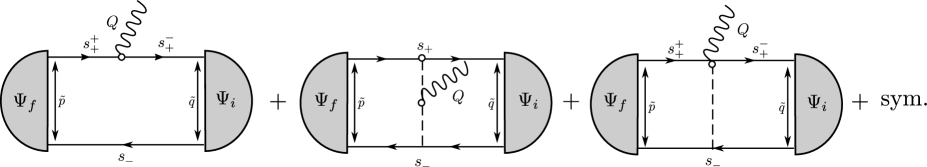
Figure 3: Diagrams relevant for the calculation of the pion form factor in the truncation employed herein, as determined by the gauging method. The impulse approximation implies considering the first diagram and the corresponding permutation only.

III.1 Interaction Kernels

The interaction kernel $K$ in eqs. (III) and (10) encodes all possible interactions processes between a quark and an antiquark. In a diagrammatic representation, it contains a sum of infinitely many terms. In practical calculations, the expansion of the interaction kernel must be truncated to a sum of a finite number of terms, chosen such that the relevant dynamics and global symmetries are correctly implemented. Chiral symmetry and its dynamical breaking ensures that pions are massless bound states in the chiral limit as a consequence of Goldstone’s theorem. On the other hand, U(1) vector symmetry ensures charge conservation in electromagnetic processes. Chiral symmetry will be correctly implemented in the DSE/BSE formalism only if the kernel fulfills the axial-vector Ward-Takahashi identity (Ax-WTI)

$$i\Sigma_{ar}\left(p_{+}\right)\gamma^{5}_{rb}t^{i}_{\alpha\beta}+i\gamma^{5}_{ar}\Sigma_{rb}\left(p_{-}\right)t^{i}_{\alpha\beta}=\int_{q}K^{r\rho,s\sigma}_{a\alpha,b\beta}\left(Q,p,q\right)\left[i~{}t^{i}_{\rho\nu}\gamma^{5}_{rn}S_{n\nu,s\sigma}\left(q_{-}\right)+i~{}S_{r\rho,e\epsilon}\left(q_{+}\right)\gamma^{5}_{es}~{}t^{i}_{\epsilon\sigma}\right]~{},$$ (14)

with $\Sigma$ the quark self-energy and $v_{\pm}=v\pm Q/2$. Similarly, vector symmetry will be correctly implemented if the kernel satisfies the vector Ward-Takahashi identity (V-WTI)

$$i\Sigma_{ab}\left(p_{+}\right)t^{i}_{\alpha\beta}-i\Sigma_{ab}\left(p_{-}\right)t^{i}_{\alpha\beta}=\int_{q}K^{r\rho,s\sigma}_{a\alpha,b\beta}\left(Q,p,q\right)\left[i~{}t^{i}_{\rho\nu}S_{r\nu,s\sigma}\left(q_{-}\right)-i~{}S_{r\rho,s\epsilon}\left(q_{+}\right)~{}t^{i}_{\epsilon\sigma}\right]~{}.$$ (15)

In DSE/BSE studies the most widely used truncation is the so-called rainbow-ladder (RL) truncation, whereby the BSE kernel consists of a vector-vector gluon exchange, namely (omitting again color indices)

$$K^{r\rho,s\sigma}_{a\alpha,b\beta}\left(Q,p,q\right)=\alpha\left(k^{2}\right)\gamma^{\mu}_{ar}\gamma^{\nu}_{sb}D^{\mu\nu}\left(k\right)\delta^{\alpha\rho}\delta^{\sigma\beta}~{},$$ (16)

with $k=p-q$ the gluon momentum. In order to preseve the Ax-WTI and V-WTI the kernel (16) is used in combination with a truncated quark DSE, defined by the replacement

$$Z_{1f}\gamma_{\mu}Z(k^{2})\Gamma_{\nu}^{\text{qgl}}(q,p)\rightarrow Z_{2}^{2}\gamma_{\mu}4\pi\alpha(k^{2})\gamma_{\nu}$$ (17)

such that $\alpha(k^{2})$ provides an effective coupling that describes the strength of the quark-antiquark interaction. To parametrise this effective interaction we use the Maris-Tandy model Maris:1997tm ; Maris:1999nt

$$\alpha(q^{2})=\pi\eta^{7}\left(\frac{q^{2}}{\Lambda^{2}}\right)^{2}e^{-\eta^{2}\frac{q^{2}}{\Lambda^{2}}}+\frac{2\pi\gamma_{m}\big{(}1-e^{-q^{2}/\Lambda_{t}^{2}}\big{)}}{\textnormal{ln}[e^{2}-1+(1+q^{2}/\Lambda_{QCD}^{2})^{2}]}~{},$$ (18)

where the second term on the right-hand side reproduces the one-loop QCD behavior of the quark propagator in the ultraviolet, and the Gaussian term provides enough interaction strength for dynamical chiral symmetry breaking to take place. The model parameters $\Lambda$ and $\eta$ are determined as explained in the next section. The scale $\Lambda_{t}=1$ GeV is introduced for technical reasons and has no impact on the results. For the anomalous dimension we use $\gamma_{m}=12/(11N_{C}-2N_{f})=12/25$ with $N_{f}=4$ flavours and $N_{c}=3$ colours. For the QCD scale we use $\Lambda_{QCD}=0.234$ GeV.

In the RL truncation, bound states cannot develop a decay width, correspondingly their masses are real numbers. Note that bound states, determined as solutions of BSEs, appear as poles in Green’s functions with the corresponding quantum numbers. In the RL approximation these poles occur for real (and in the convention employed here, negative) momentum-squared values in certain kinematic configurations. In particular, the photon being described by a vector field, electrically neutral vector mesons appear as poles of the quark-photon vertex. In the RL approximation these poles are located at negative and real values of $Q^{2}$ (for which $M^{2}=-Q^{2}$ with $M$ being the mass of the vector meson). Such poles in the quark-photon vertex also manifest as poles in the calculation of time-like form factors, in contradiction with phenomenology. Generally speaking, any physical phenomenon that is triggered by the presence of virtual intermediate particles, as, e.g., decays, will be absent from any calculation using the RL truncation only.

It is possible to improve the RL truncation in this respect by re-introducing the presence of intermediate particles explicitly. The simplest implementation of such an idea was introduced in Fischer:2007ze ; Fischer:2008sp , where, based on the role of the pion as lightest hadron, explicit pion-quark interactions were introduced in the truncated quark DSE and in the BSE kernel $K$, with the pion-quark interaction vertex given by the pion Bethe-Salpeter amplitude $\Gamma$, calculated consistently via a truncated BSE. The corresponding additional BSE kernels are given in Appendix A and shown in Fig. 8, and the technical difficulties arising for time-like momenta when those kernels are used in BSEs have been described in detail in Miramontes:2019mco . This type of kernels enable the possibility of intermediate virtual decays in the BSE interaction kernel to occur. As a consequence, certain BSE solutions signal a finite decay width and thus represent (a) hadron resonance(s). E.g., the description of the $\rho$-meson as a finite-width resonance is then mostly due to the intermediate process $\rho\rightarrow\pi\pi$ (see Williams:2018adr for a treatment in the here discussed approach as well as Jarecke:2002xd ; Mader:2011zf and references therein for respective calculations based on DSEs and BSEs), the partial decay width to the latter process representing more than 99%  of the total $\rho$ decay width. Additionally, and thereby completing the physical effects of intermediate virtual $\pi\pi$-states, in this truncation the quark-photon vertex develops a multi-particle branch cut along the negative real $Q^{2}$ axis, starting as expected at the two-pion production threshold Miramontes:2019mco . Clearly, including these two effects of the intermediate virtual $\pi\pi$-states is especially important when it comes to the calculation of the pion form factor for time-like momenta in the sub-GeV kinematic region.

We wish to stress here that, for computational feasibility, for the pion vertices in (23)–(26) we used the leading $\gamma_{5}$ component of the pion Bethe-Salpeter amplitude in the chiral limit, given by $B/f_{\pi}$ with $B$ one of the quark’s dressing functions, see Eq. (27). On the other hand, the pion amplitudes used in the form factor calculation of Eq. (19) are considered in full, including their leading and sub-leading contributions. In that regard, our calculations contain two types of treatments of pions.

Even though the “pionic” kernels (23)–(26) are phenomenologically justified and, as we will see in the next section, constitute a first step in the correct direction, it must be noted that they have not been (yet) rigorously derived from QCD. Lacking a solid quantum-field theoretical basis the use of these kernels comes with some shortcomings, especially it implies that the Ax-WTI and V-WTI are not fulfilled simultaneously. Indeed, one can choose to preserve either the Ax-WTI (and hence chiral symmetry) or the V-WTI (and hence charge conservation), but not both Fischer:2007ze ; Miramontes:2019mco . It turns out, however, that the respective violation of either of them induce typically only small errors in physical observables, as we will demonstrate for some quantities in the next section.

III.2 Form factor calculation

Meson form factors are extracted from a current $J^{\mu}$ encoding the coupling of a meson to an external electromagnetic current. In the BSE framework, the current is calculated by means of the coupling of an external photon to each of the constituents of the bound state, as specified by a procedure known as gauging and developed in Haberzettl:1997jg ; Kvinikhidze:1998xn ; Kvinikhidze:1999xp ; Oettel:1999gc ; Oettel:2000jj . The conserved current $J^{\mu}$ that describes the coupling of a single photon with a quark-antiquark, a three-quark or other multi-quark system is given by,

$$J^{\mu}=\bar{\Psi}_{f}G_{0}(\mathbf{\Gamma}^{\mu}-K^{\mu})G_{0}\Psi_{i}~{},$$ (19)

with $\Psi_{i,f}$ the incoming and outgoing Bethe-Salpeter amplitudes of the meson, the baryon or some other multi-quark state, and $G_{0}$ represents the appropriate product of dressed quark propagators. This equation is shown diagrammatically for the quark-antiquark–meson case in Fig. 3. The term $\Gamma^{\mu}$ represents the impulse approximation diagrams where the photon couples to the valence quarks only

$$\mathbf{\Gamma}^{\mu}=\left(S^{-1}\otimes S^{-1}\right)^{\mu}=\Gamma^{\mu}\otimes S^{-1}+S^{-1}\otimes\Gamma^{\mu}~{},$$ (20)

with $\Gamma^{\mu}$ the quark-photon vertex. The term $K^{\mu}$ describes the interaction of the photon with the Bethe-Salpeter kernel, which in our truncation includes the coupling of the photon to the quark-pion vertex and to the propagating pions (second and third diagram in Fig. 3). Including both terms in (19) is necessary in order to implement current conservation precisely. Note that the s- and u-channel pion decay terms (most right diagram in Fig. 8) do not contribute to the term $K^{\mu}$, also not via seagulls, the reason being that trying to include them would leave a $\pi$ $\pi$ $\pi$ amplitude on one side of the respective full diagram. However, the new vertices appearing in the term $K^{\mu}$, the coupling of the photon to the quark-pion vertex and to the propagating pions, represent an enormous computational challenge. Given the exploratory purpose of the present calculation, we thus decided to omit the coupling of the photon to the quark-pion vertex and to the propagating pions, and to consider the impulse diagram only (first diagram in Fig. 3). As we will show in the next section, the thereby implied violation of charge conservation is at the level of approximately one percent.

IV Results

Following the formalism sketched above, we have calculated the pion electromagnetic form factor in the time-like $Q^{2}<0$ domain. For comparison with previous calculations we will also show results in the space-like $Q^{2}>0$ domain.

In our discussion in the preceding section, it remained to be explained how the parameters $\eta$ and $\Lambda$ of our interaction model (18) as well as the value of the current quark mass are fixed. It is customary in studies using the RL truncation to adjust those parameters such that the pion decay constant agrees with the experimental value. In ref. Miramontes:2019mco the quark-photon vertex has been calculated for the first time with the above discussed interaction kernels taken into account and also used herein. The parameters, including the isospin symmetric light quark current mass $m_{q}$, were adjusted such that the pion mass and decay constant as well as the $\rho$-meson mass have been correctly reproduced in the employed approximation. Here, only the gluon- and pion-exchange kernels need to be used for fixing the parameters because the pion decay kernels (25) and (26) do not contribute to the pion BSE.

For the present exploratory calculation, we choose to adjust the parameters in a slightly different and simpler manner, especially as we aim at a qualitative understanding of the physical mechanisms involved in determining the shape of the pion form factor, and not so much at achieving an accurate quantitative agreement with experiment. First, we set initially $\eta=1.5$. Second, although we assume (confirmed by our calculation) that the pion-decay kernels will not only move the $\rho$-meson pole into the complex plane but also shift down its real value, we nevertheless adjust the parameter $\Lambda$ such that we obtain a $\rho$-meson mass close to the phenomenological value already in the calculations with gluon- and pion-exchange kernels only. Third, we require to reproduce a quite accurate value for the pion decay constant. Finally, we adjust $m_{q}$ to obtain the correct value for the pion mass as well. In this way we chose the model parameters to be $\eta=1.5$, $\Lambda=0.78$ GeV and $m_{q}=6.8$ MeV at a renormalisation scale $\mu=19$ GeV. As a rudimentary test of model dependence we additionally perform the calculations for $\eta=1.6$ as well (keeping $\Lambda$ and $m_{q}$ unchanged). The results for the pion mass and decay constant as well as for the $\rho$-meson and $\omega$-meson masses, without the pion decay kernels being taken into account, are shown in Tab. 1.

Table 1: The pion mass $m_{\pi}$, the pion decay constant $f_{\pi}$, the $\rho$-meson and $\omega$-meson masses $m_{\rho}$ and $m_{\omega}$ for the two different parameterizations of the model used herein and for the case with rainbow-ladder and pion-exchange kernels but without decay kernels are shown. The light quark mass has been set to $m_{q}=0.0068~{}$GeV. The rightmost column displays the extracted $\rho$-meson pole position defined as $M_{pole}^{2}=M_{\rho}^{2}-iM_{\rho}\Gamma_{\rho}$, as discussed in the text. All values for dimensionful quantities are given in GeV.

$\Lambda=0.78$	$m_{\pi}$	$f_{\pi}$	$m_{\rho}$	$m_{\omega}$	$M_{\rho}$	$\Gamma_{\rho}$
$\eta=1.5$	0.139	0.138	0.768	0.778	0.750	0.100
$\eta=1.6$	0.126	0.138	0.774	0.784	0.759	0.105

As mentioned in the previous section, the full QCD quark-photon vertex possesses poles reflecting the masses and widths of the electrically neutral vector meson resonances. Correspondingly, and as discussed in detail in refs. Miramontes:2019mco ; Williams:2018adr , a solution for the quark-photon vertex in the DSE/BSE framework allows to extract the $\rho$-meson mass and width via the position of the poles of the vertex dressing functions. For the RL truncation as well as for the RL plus pion exchange approximation this pole is located on the real negative $Q^{2}$ axis indicating that the $\rho$ mesons were stable for those truncations. Including the $s$- and $u$-channel decay kernels (25) and (26), the pole of the dressing functions moves into the complex plane and can be extracted from the data on the real axis via a Padé fit. Parametrising the pole position as $M_{pole}^{2}=M^{2}_{\rho}-iM_{\rho}\Gamma_{\rho}$, we extract the corresponding results for the $\rho$-meson mass and width, $M_{\rho}$ and $\Gamma_{\rho}$ for this truncation (see Tab. 1) in reasonable agreement with the experimental values. Hereby, it has to be noted that underestimating the $\rho$-meson width does not come unexpected because taking into account only the leading $\gamma_{5}$ component of the pion Bethe-Salpeter amplitude in the kernels (23)–(26) misses some strengths therein. Whether considering in addition also the sub-leading pion amplitudes will provide a much better result for the $\rho$-meson width can only be answered by performing the corresponding calculation. This computation is then, however, an order of magnitude more expensive than the present exploratory calculation.

It is interesting to note that the pion exchange kernels lift the degeneracy in between the isovector $\rho$- and the isosinglet $\omega$-meson present at the level of RL calculations the interaction kernels of which are flavour blind and thus flavour U(2) (resp., flavour U$(N_{f})$) symmetric. The pion exchange kernels lead to a splitting such that $m_{\omega}-m_{\rho}=10$ MeV which compares favorably with the experimental splitting of 7 - 8 MeV.

We turn now to the calculation of the pion form factor.

As already indicated in the previous section, there are, besides restricting to the leading pion amplitude in the kernels(23)–(26), two major approximations that we must perform in order to keep the calculation technically manageable. First, using the decay kernels as described in this work entails that one must choose whether the axial-vector or the vector WTI are preserved while the other one is violated. Following Miramontes:2019mco we choose to preserve the vector identity. A violation of the axial-vector WTI is manifested, among others, in the pion not being massless in the chiral limit, and therefore the value of the current mass for which the pion becomes massless allows for a quantification of the violation of the axial-vector WTI. In Fig. 4 we therefore show the evolution of the pion mass with varying $m_{q}$ in the employed truncation. First, the relation is linear as expected from the Gell-Mann–Oakes–Renner relation which is a direct consequence of the dynamical breaking of chiral symmetry. Second, the pion does not become massless in the chiral limit but for a value of the current mass $m_{q}^{(0)}$($\mu=19$ GeV) = 3 MeV. On the one hand, this explains the relatively large value of $m_{q}$($\mu=19$ GeV) = 6.8 MeV we needed to obtain the correct pion mass: The related explicitly chiral-symmetry-breaking term is $m_{q}-m_{q}^{(0)}$ = 3.8 MeV, and thus much closer to what is expected from the known parameters of QCD. Second, as the masses of the vector mesons depend linearly on the current mass the induced error on $m_{\rho}$ and $m_{\omega}$ is of the order of $m_{q}^{(0)}$ = 3 MeV, and thus it is as small or even smaller than other uncertainties in our calculation of the vector meson masses.

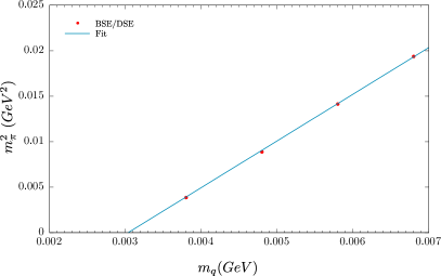
Figure 4: The pion mass squared $m_{\pi}^{2}$ vs. the current mass $m_{q}$($\mu=19$ GeV) for the employed truncation.

Second, in the calculation of the form factor we use the impulse approximation which, in this context, implies neglecting the second and third diagrams in Fig. 3. The consequence of discarding diagrams is the violation of charge conservation or, equivalently, a deviation from $F_{\pi}(0)=1$. As can be seen in the inset in Fig. 5, this effect is of the order of $\sim 1\%$ only.

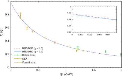
Figure 5: Pion form factor in the spacelike $Q^{2}>0$ domain for the model parameters $\eta=1.5$ and $\eta=1.6$ as described in the text and compared to experimental data.

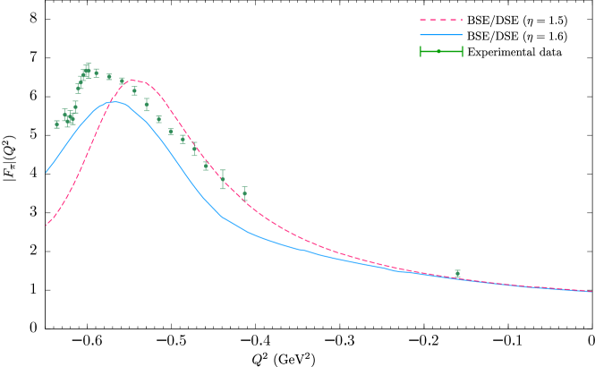
Figure 6: Absolute value of the pion form factor in the time-like $Q^{2}<0$ domain for the model parameters $\eta=1.5$ and $\eta=1.6$ as described in the text and compared to experimental data.

As can be also seen from Fig. 5, the results for the pion form factor in the space-like $Q^{2}>0$ regime are practically independent from the value of the $\eta$ parameter of the model. Even more remarkable is the fact that our calculation shows a very good agreement with experimental data in the space-like domain even though, as evident from the above discussion, we aimed at including all physical effects which are important in the time-like regime. An interpretation of this result in view of the dispersion relation (4) provides an indication that the imaginary part in the time-like region is precisely enough reproduced to provide very good results for the space-like form factor.

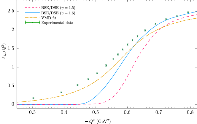
Figure 7: Phase of the pion form factor in the time-like $Q^{2}<0$ domain for the model parameters $\eta=1.5$ and $\eta=1.6$ as described in the text and compared to experimental data on pion-pion phase shift.

We show our results for the pion form factor for time-like ($Q^{2}<0$) virtualities in Figs. 6 and 7. As discussed in the previous section, as a consequence of the decay kernels in our truncation, the pion form factor develops a branch cut along the real negative axis starting from the two-pion threshold $Q^{2}=-4m_{\pi}^{2}$, induced by the corresponding cut in the quark-photon vertex Miramontes:2019mco . Hence, in that region the (complex) form factor is defined from its analytic continuation as $F(Q^{2}+i\epsilon)$. In the numerical calculations we have typically chosen $\epsilon=0.0001$ GeV² after verifying that this value is small enough to not disturb the presented results. In Fig. 6 we present the absolute value for the model parameter $\eta=1.5$ and $\eta=1.6$, with the remaining model parameters kept constant, as discussed above. As a manifestation of the fact that the $\rho$-meson pole in the quark-photon vertex moves into the complex plane when the decay kernels are included in the calculation, the pion form factor develops a bump on the real and negative $Q^{2}$ axis with an approximately correct height and width. Therefore our calculation overcomes a major deficiency of the RL truncation, without or even with the pion exchange term, for which the form factor diverges instead at the $Q^{2}$-value corresponding to the $\rho$-meson mass in those truncations, see e.g. Maris:1999bh ; Krassnigg:2004if ; Eichmann:2019tjk . This constitutes already one main result of the here presented investigation.

We note, however, that, contrary to the results for space-like regime, the position and height of the bump of the form factor depends strongly on the value of the $\eta$ parameter shape of the form factor. Of course, this reflects the different positions of the $\rho$-meson pole, cf. Tab. 1. Nevertheless, there are features that appear to be independent of $\eta$, most prominently that the height of the bump is underestimated. As expected from the discussion in Sec. II the form factor behaves smoothly after the bump, in contrast to the sharp dip in the experimental data. Even though an unambiguous analysis of the origin of such discrepancies can only result from the inclusion of all relevant physical mechanisms in our calculations, it is evident from the analysis performed in Sec. II that one of the main missing elements is the $\rho$-$\omega$ mixing due to isospin breaking, which is completely absent in the present study.

Particularly sensitive to the deficiencies of our truncation is the phase of the form factor, shown in Fig. 7. Even though our data shows the expected behaviour near the resonance value, it severely underestimates the experimental data, particularly in the elastic region. This is a manifestation of the absence of some hadronic effects in our approximation scheme, which only includes those stemming from the resonance complex pole in the quark-photon vertex and the $\rho\rightarrow\pi\pi$ induced branch cut. In addition to the isospin breaking effects discussed above, and which would be more relevant in the region above the resonance, the impulse approximation used in our calculation of the form factor entails that effects coming from the coupling of the photon to the intermediate hadrons, via its coupling to the exchanged pion or to the quark-pion vertex (see Fig. 3), are missing. It has been shown Cotanch:2002vj that considering only impulse-like diagrams leads to a very small pion-pion scattering amplitude in the elastic region in the isospin $I=1$ channel. This, due to unitarity, implies a very small value of the imaginary part of the pion form factor in the elastic region (which is, in fact, what we observe) which translates into a very small phase, as seen in Fig. 7 (and as could be inferred from Watson’s theorem).

Last but not least, we are comparing Padé fits, resp. rational fits of the order (3,3), for the real part and for the imaginary part of the form factor to the expression (8). Trying first,

$$Re\,F_{\pi}(Q^{2})-F_{\pi}(0) \approx -\frac{a_{0}+a_{1}Q^{2}+a_{2}(Q^{2})^{2}+a_{3}(Q^{2})^{3}}{b_{0}+b_{1}Q^{2}+b_{2}(Q^{2})^{2}+b_{3}(Q^{2})^{3}}$$

$$Im\,F_{\pi}(Q^{2}) \approx \frac{c_{0}+c_{1}Q^{2}+c_{2}(Q^{2})^{2}+c_{3}(Q^{2})^{3}}{d_{0}+d_{1}Q^{2}+d_{2}(Q^{2})^{2}+d_{3}(Q^{2})^{3}}\,,$$

we obtain tiny values for the coefficients $a_{0}$, $a_{3}$, $b_{3}$, $c_{0}$, $c_{3}$ and $d_{3}$. Note that this confirms the structure expected from the VMD form (8). We repeated the fits for

$$Re\,F_{\pi}(Q^{2})-F_{\pi}(0) \approx -\frac{a_{1}Q^{2}+a_{2}(Q^{2})^{2}}{b_{0}+b_{1}Q^{2}+b_{2}(Q^{2})^{2}}$$

$$Im\,F_{\pi}(Q^{2}) \approx \frac{c_{1}Q^{2}+c_{2}(Q^{2})^{2}}{d_{0}+d_{1}Q^{2}+d_{2}(Q^{2})^{2}}\,.$$ (22)

The coefficients resulting from these fits as well as the ones resulting from expression (8) are given in table 2. From this we conclude that the expression based on the VMD is an astonishingly good representation of our results. Therefore, our investigation makes it plausible that the VMD picture can be derived from QCD. At least, the results of the here presented microscopic approach give a strong hint into this direction.

Table 2: The coefficients of the rational fits to the pion form factor as discussed in the text. All values for dimensionful quantities are given in GeV.

	$\eta$ =1.5	$\eta$ =1.6	Eq. (8)
$a_{1}$	0.5587	0.4149	0.72
$a_{2}$	0.8828	0.6827	1.2
$b_{0}$	0.3600	0.3600	0.36
$b_{1}$	1.2307	1.2517	1.2
$b_{2}$	1.0722	1.1000	1.037
$c_{1}$	0.0591	0.0997	0
$c_{2}$	0.1295	0.2383	0.2308
$d_{0}$	0.3600	0.3600	0.36
$d_{1}$	1.1924	1.2464	1.2
$d_{2}$	0.9973	1.0916	1.0037

V Conclusions and outlook

In this work we have presented an exploratory study of the pion form factor in the DSE/BSE approach. Our focus has been to explore how the interplay between hadron structure (as described by form factors) and the hadron spectrum (as described by resonance masses and widths) can be realised in the microscopic approach presented herein. In particular, we focused on the effect of intermediate pions in the BSE interaction kernel, the inclusion of which is sufficient to describe the $\rho$ meson as a resonance Williams:2018adr . As elucidated by the detailed analysis in the last section our calculation represents a verification of the vector meson dominance picture and provides an explanation how at the quark level vector meson dominance becomes effective. A more complete calculation than the one presented here might then actually provide a derivation of vector meson dominance from QCD.

Despite the fairly drastic approximations used in this preliminary study, the agreement with experiment is remarkable. On the space-like side our calculations agree with experimental data at the quantitative level. For time-like momentum transfers the agreement is mostly qualitative and consistent with the fact that in our approximation scheme time-like physics is dominated by the lowest-lying $\rho$-meson resonance only. The absolute value of the calculated form factor features a bump at approximately the correct $Q^{2}$ region as caused by a resonance pole. Our result lacks, however, other features such as those caused by the isospin-breaking $\rho$-$\omega$ mixing and interference. The phase of the form factor also shows deficiencies caused by the employed impulse approximation. However, the overall qualitatively correct behaviour is, nevertheless, very encouraging for future studies on time-like phenomenology with BSE methods as it shows that the necessary computational techniques are getting more and more under control, and that within a functional-method-based bound-state approach to QCD direct calculations in the time-like regime are becoming feasible.

Among the different physical mechanisms absent in our calculation, the most relevant one appears to be isospin breaking by the light quarks’ masses and electric charges, and the different phenomena associated with it. The presented exploratory calculation paved the way to include in a bound-state approach formulated in QCD degrees of freedom the effects of isospin violation, and hereby most prominently $\rho$-$\omega$ mixing, on the time-like pion electromagnetic form factor. Thus including isospin violation in a BSE approach is the topic of ongoing work. A further related topic is the study of the form factor for the coupling of a photon to three pions. On the one hand, this process is of special theoretical interest because the related form factor is at the soft point completely determined by the Abelian chiral anomaly. On the other hand, data of the COMPASS experiment are currently analysed Dominik , and therefore experimental data for this form factor in the time-like region will become available. Combing previous studies in the DSE/BSE approach for the space-like $\gamma\pi\pi\pi$ form factor Alkofer:1995jx ; Bistrovic:1999dy ; Cotanch:2003xv ; Benic:2011rk ; Eichmann:2011ec with the techniques of the here presented calculation will thus enable a respective investigation of this form factor.

Another aspect we want to investigate is how to realise the idea of decay kernels like (25) and (26) in a baryon bound state equation. This is a necessary step in order to tackle time-like nucleon form factors in the DSE/BSE approach, which is one of our major goals due to the increased effort and interest from the experimental side in highly precise measurements over a wide kinematical domain of the nucleon form factors.

Appendix A Interaction kernels

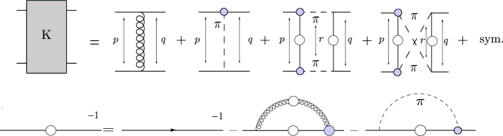
Figure 8: Truncations used herein for the BSE interaction kernel $K$ (upper diagram) and the quark DSE one (lower diagram). In the upper diagram, the terms on the right-hand side correspond to the rainbow-ladder, pion exchange, and s- and u-channel pion decay contributions to the truncation, respectively. The s- and u-channel pion decay terms do not contribute to the quark DSE.

The BSE kernel representing the exchange of an explicit pionic degrees of freedom as defined in Fischer:2007ze ; Fischer:2008sp reads

$$K^{(t)~{}ut}_{rs}(q,p;P)=$$

$$~{}~{}~{}~{}~{}~{}~{}~{}~{}~{}~{}\frac{C}{4}[\Gamma_{\pi}^{j}]_{ru}\left(\frac{p+q-P}{2};p-q\right)[Z_{2}\gamma^{5}]_{ts}D_{\pi}(p-q)$$

$$~{}~{}~{}~{}~{}~{}~{}~{}+\frac{C}{4}[\Gamma_{\pi}^{j}]_{ru}\left(\frac{p+q-P}{2};q-p\right)[Z_{2}\gamma^{5}]_{ts}D_{\pi}(p-q)$$

$$~{}~{}~{}~{}~{}~{}~{}~{}+\frac{C}{4}[Z_{2}\gamma^{5}]_{ru}[\Gamma_{\pi}^{j}]_{ts}\left(\frac{p+q+P}{2};p-q\right)D_{\pi}(p-q)$$

$$~{}~{}~{}~{}~{}~{}~{}~{}+\frac{C}{4}[Z_{2}\gamma^{5}]_{ru}[\Gamma_{\pi}^{j}]_{ts}\left(\frac{p+q+P}{2};q-p\right)D_{\pi}(p-q)~{},$$ (23)

in combination with the following truncation of the quark DSE

$$S^{-1}(p) = S^{-1}(p)^{RL}-\frac{3}{2}\int_{q}\Bigg{[}Z_{2}\gamma_{5}S(q)\Gamma_{\pi}\left(\frac{p+q}{2},q-p\right)$$ (24)

$$+Z_{2}\gamma_{5}S(q)\Gamma_{\pi}\left(\frac{p+q}{2},p-q\right)\Bigg{]}\frac{D_{\pi}(k)}{2}~{},$$

with $S^{-1}(p)^{RL}$ being the right-hand-side of the quark DSE in the RL truncation with the gluon-mediated interaction as described in Sect. III. In Eqs. (23) and (24) the pion propagator is taken as $D_{\pi}(k)=(k^{2}+m_{\pi}^{2})^{-1}$. The factor $3/2$ in Eq. (24) originates from the flavour traces, and in the same way the factor $C$ in (23) should be obtained. When done in the quark-photon vertex, the flavour factor leads to $C=+3/2$. However, such value of $C$, violates the Ax-WTI while preserving the V-WTI. Since the V-WTI is related to charge conservation in electromagnetic form factors, we use $C=+3/2$ at the expense of violating the Ax-WTI. Herein, the quark-pion vertex $\Gamma_{\pi}$ is taken to be the pion Bethe-Salpeter amplitude.

The pions in the kernel can also appear in the s- and u- channels Fischer:2007ze . We used here a version of the kernels slightly different to the one in Fischer:2007ze in order to be consistent with the construction for the t-channel, where one of the pion vertices is kept bare and the kernel is then symmetrised. They read

$$K^{(s)~{}he}_{da}(q,p,r;P)=~{} \frac{C}{2}~{}D_{\pi}\left(\frac{P+r}{2}\right)D_{\pi}\left(\frac{P-r}{2}\right)~{}\left[[Z_{2}\gamma_{5}]_{dc}S_{cb}\left(p-\frac{r}{2}\right)[Z_{2}\gamma_{5}]_{ba}\right.$$

$$~{}~{}~{}~{}\times[\Gamma_{\pi}^{j}]_{hg}\left(q-\frac{P}{4}-\frac{r}{4};\frac{r-P}{2}\right)S_{gf}\left(q-\frac{r}{2}\right)[\Gamma_{\pi}^{j}]_{fe}\left(q+\frac{P}{4}-\frac{r}{4};-\frac{P+r}{2}\right)$$

$$+~{}[\Gamma_{\pi}^{j}]_{dc}\left(p+\frac{P}{4}-\frac{r}{4};\frac{P+r}{2}\right)S_{cb}\left(p-\frac{r}{2}\right)[\Gamma_{\pi}^{j}]_{ba}\left(p-\frac{P}{4}-\frac{r}{4};\frac{P-r}{2}\right)$$

$$~{}~{}~{}~{}\left.\times[Z_{2}\gamma_{5}]_{hg}S_{gf}\left(q-\frac{r}{2}\right)[Z_{2}\gamma_{5}]_{fe}\right]~{},$$ (25)

and

$$K^{(u)~{}he}_{da}(q,p,r;P)=~{} \frac{C}{2}~{}D_{\pi}\left(\frac{P+r}{2}\right)D_{\pi}\left(\frac{P-r}{2}\right)~{}\left[[Z_{2}\gamma_{5}]_{dc}S_{cb}\left(p+\frac{r}{2}\right)[Z_{2}\gamma_{5}]_{ba}\right.$$

$$~{}~{}~{}~{}\times[\Gamma_{\pi}^{j}]_{hg}\left(q-\frac{P}{4}-\frac{r}{4};\frac{r-P}{2}\right)S_{gf}\left(q-\frac{r}{2}\right)[\Gamma_{\pi}^{j}]_{fe}\left(q+\frac{P}{4}-\frac{r}{4};-\frac{P+r}{2}\right)$$

$$+~{}[\Gamma_{\pi}^{j}]_{dc}\left(p+\frac{P}{4}+\frac{r}{4};\frac{P-r}{2}\right)S_{cb}\left(p+\frac{r}{2}\right)[\Gamma_{\pi}^{j}]_{ba}\left(p-\frac{P}{4}+\frac{r}{4};\frac{P+r}{2}\right)$$

$$~{}~{}~{}~{}\left.\times[Z_{2}\gamma_{5}]_{hg}S_{gf}\left(q-\frac{r}{2}\right)[Z_{2}\gamma_{5}]_{fe}\right]~{},$$ (26)

where now $r$ is an additional integration momentum in the BSE (cf. Eqs.(III) or (10)). The resulting truncation of the BSE kernel and the quark DSE is shown in Fig. 8.

The inclusion of the two kernels given in equations (25) and (26) generates a highly non-trivial analytic structure of the integrand of the BSE, induced by the intermediate pions going potentially on-shell as well as by singularities in the quark propagators, see ref. Miramontes:2019mco for details where also the techniques for finding viable contour deformations for performing the numerical integrations in a mathematically correct way are described.

The pion Bethe-Salpeter amplitude possesses four tensor components. Hereby, only one is generically small such that for a precise calculation of pion properties it would be necessary to take into account three of them, namely the leading pseudoscalar term and two subleading ones related to the axialvector structure. However, using in the above described kernels three amplitudes for every pion Bethe-Salpeter amplitude in these expressions is numerically by an order of magnitude more expensive and far beyond the scope of the present study. Having restricted to the leading component of the pion amplitude in the kernels (23) and (26) one can further exploit that this leading amplitude may be well approximated using the chiral limit value of the quark dressing function $B(p^{2})$ and normalize the amplitude by dividing through the pion decay constant $f_{\pi}$,

$$\Gamma_{\pi}^{i}(p;P)=\tau^{i}\gamma_{5}\frac{B(p^{2})}{f_{\pi}}\,.$$ (27)

For light quarks the difference between calculated leading order amplitude and this approximation is at the level of a few percent, see, e.g., Fischer:2008wy and references therein. Therefore we use this simplified form.

Appendix B Poles of the quark propagator

In the truncations of the quark DSE used in this paper, the quark propagator features pairs of complex conjugate poles in the complex plane (see, e.g. Windisch:2016iud ). In order to facilitate the use of the quark propagators and easily identify the analytic structures generated by those poles in the form factor and vertex calculations, it is useful to parametrise the quark propagator simply as a sum of poles (see e.g. El-Bennich:2016qmb )

$$S(p) = -i\ooalign{\hfil/\hfil\crcr$p$}\sigma_{v}(p^{2})+\sigma_{s}(p^{2})\,,$$ (30)

$$\sigma_{v}(p^{2}) = \sum_{i}^{n}\left[\frac{\alpha_{i}}{p^{2}+m_{i}}+\frac{\alpha_{i}^{\ast}}{p^{2}+m_{i}^{\ast}}\right]\,,$$

$$\sigma_{s}(p^{2}) = \sum_{i}^{n}\left[\frac{\beta_{i}}{p^{2}+m_{i}}+\frac{\beta_{i}^{\ast}}{p^{2}+m_{i}^{\ast}}\right]~{},$$ (31)

where the parameters $m_{i}$, $\alpha_{i}$, $\beta_{i}$ can be obtained by fitting the corresponding quark DSE solution along the $p^{2}$ real axis or, alternatively, on a parabola in the complex plane that does not enclose the poles.

In the numerical solution of the quark DSE in the complex plane we tested fits with one real and one pair of complex conjugated poles, with two pairs of complex conjugated poles, and with three pairs of complex conjugated poles. Based on this tests we concluded that $n=2$ pairs of complex conjugated poles provided a precise fit, and as the use of three pairs of poles did not provide any further improvement, the reported calculations have been performed based on fits with two pairs of poles.

References

- (1) W. Melnitchouk, R. Ent and C. Keppel, Phys. Rept. 406, 127-301 (2005) doi:10.1016/j.physrep.2004.10.004 [arXiv:hep-ph/0501217 [hep-ph]].
- (2) I. C. Cloet and C. D. Roberts, Prog. Part. Nucl. Phys. 77 (2014) 1 doi:10.1016/j.ppnp.2014.02.001 [arXiv:1310.2651 [nucl-th]].
- (3) G. Eichmann, H. Sanchis-Alepuz, R. Williams, R. Alkofer and C. S. Fischer, Prog. Part. Nucl. Phys. 91 (2016) 1 doi:10.1016/j.ppnp.2016.07.001 [arXiv:1606.09602 [hep-ph]].
- (4) M. Q. Huber, Phys. Rept. 879, 1 (2020) doi:10.1016/j.physrep.2020.04.004 [arXiv:1808.05227 [hep-ph]].
- (5) H. Sanchis-Alepuz and R. Williams, Comput. Phys. Commun. 232 (2018) 1 doi:10.1016/j.cpc.2018.05.020 [arXiv:1710.04903 [hep-ph]].
- (6) M. Q. Huber, C. S. Fischer and H. Sanchis-Alepuz, Eur. Phys. J. C 80, no.11, 1077 (2020) doi:10.1140/epjc/s10052-020-08649-6 [arXiv:2004.00415 [hep-ph]].
- (7) K. Langfeld, R. Alkofer and P. A. Amundsen, Z. Phys. C 42, 159-165 (1989) doi:10.1007/BF01565138
- (8) C. D. Roberts, Nucl. Phys. A 605, 475-495 (1996) doi:10.1016/0375-9474(96)00174-1 [arXiv:hep-ph/9408233 [hep-ph]].
- (9) P. Maris and P. C. Tandy, Phys. Rev. C 62, 055204 (2000) doi:10.1103/PhysRevC.62.055204 [arXiv:nucl-th/0005015 [nucl-th]].
- (10) L. Chang, I. C. Cloët, C. D. Roberts, S. M. Schmidt and P. C. Tandy, Phys. Rev. Lett. 111, no.14, 141802 (2013) doi:10.1103/PhysRevLett.111.141802 [arXiv:1307.0026 [nucl-th]].
- (11) D. Nicmorus, G. Eichmann and R. Alkofer, Phys. Rev. D 82, 114017 (2010) doi:10.1103/PhysRevD.82.114017 [arXiv:1008.3184 [hep-ph]].
- (12) G. Eichmann, Phys. Rev. D 84, 014014 (2011) doi:10.1103/PhysRevD.84.014014 [arXiv:1104.4505 [hep-ph]].
- (13) G. Eichmann and C. S. Fischer, Eur. Phys. J. A 48, 9 (2012) doi:10.1140/epja/i2012-12009-6 [arXiv:1111.2614 [hep-ph]].
- (14) H. Sanchis-Alepuz, R. Williams and R. Alkofer, Phys. Rev. D 87, no.9, 096015 (2013) doi:10.1103/PhysRevD.87.096015 [arXiv:1302.6048 [hep-ph]].
- (15) H. Sanchis-Alepuz, R. Alkofer and C. S. Fischer, Eur. Phys. J. A 54, no.3, 41 (2018) doi:10.1140/epja/i2018-12465-x [arXiv:1707.08463 [hep-ph]].
- (16) G. Barucca et al. [PANDA], [arXiv:2101.11877 [hep-ex]].
- (17) B. Ananthanarayan, I. Caprini and D. Das, Phys. Rev. D 102, no.9, 096003 (2020) doi:10.1103/PhysRevD.102.096003 [arXiv:2008.00669 [hep-ph]].
- (18) J. H. Kim and L. Resnick, Phys. Rev. D 21, 1330 (1980) doi:10.1103/PhysRevD.21.1330
- (19) R. R. Akhmetshin et al. [CMD-2], Phys. Lett. B 648, 28-38 (2007) doi:10.1016/j.physletb.2007.01.073 [arXiv:hep-ex/0610021 [hep-ex]].
- (20) D. Brömmel et al. [QCDSF/UKQCD], Eur. Phys. J. C 51, 335-345 (2007) doi:10.1140/epjc/s10052-007-0295-6 [arXiv:hep-lat/0608021 [hep-lat]].
- (21) R. Frezzotti et al. [ETM], Phys. Rev. D 79, 074506 (2009) doi:10.1103/PhysRevD.79.074506 [arXiv:0812.4042 [hep-lat]].
- (22) P. A. Boyle, J. M. Flynn, A. Juttner, C. Kelly, H. P. de Lima, C. M. Maynard, C. T. Sachrajda and J. M. Zanotti, JHEP 07, 112 (2008) doi:10.1088/1126-6708/2008/07/112 [arXiv:0804.3971 [hep-lat]].
- (23) S. Aoki et al. [JLQCD and TWQCD], Phys. Rev. D 80, 034508 (2009) doi:10.1103/PhysRevD.80.034508 [arXiv:0905.2465 [hep-lat]].
- (24) O. H. Nguyen, K. I. Ishikawa, A. Ukawa and N. Ukita, JHEP 04, 122 (2011) doi:10.1007/JHEP04(2011)122 [arXiv:1102.3652 [hep-lat]].
- (25) B. B. Brandt, A. Jüttner and H. Wittig, JHEP 11, 034 (2013) doi:10.1007/JHEP11(2013)034 [arXiv:1306.2916 [hep-lat]].
- (26) J. Koponen, F. Bursa, C. Davies, G. Donald and R. Dowdall, PoS LATTICE2013, 282 (2014) doi:10.22323/1.187.0282 [arXiv:1311.3513 [hep-lat]].
- (27) H. B. Meyer, Phys. Rev. Lett. 107, 072002 (2011) doi:10.1103/PhysRevLett.107.072002 [arXiv:1105.1892 [hep-lat]].
- (28) X. Feng, S. Aoki, S. Hashimoto and T. Kaneko, Phys. Rev. D 91, no.5, 054504 (2015) doi:10.1103/PhysRevD.91.054504 [arXiv:1412.6319 [hep-lat]].
- (29) J. Bulava, B. Hörz, B. Fahy, K. J. Juge, C. Morningstar and C. H. Wong, PoS LATTICE2015, 069 (2016) doi:10.22323/1.251.0069 [arXiv:1511.02351 [hep-lat]].
- (30) F. Erben, J. R. Green, D. Mohler and H. Wittig, Phys. Rev. D 101, no.5, 054504 (2020) doi:10.1103/PhysRevD.101.054504 [arXiv:1910.01083 [hep-lat]].
- (31) H. B. O’Connell, B. C. Pearce, A. W. Thomas and A. G. Williams, Prog. Part. Nucl. Phys. 39 (1997), 201-252 doi:10.1016/S0146-6410(97)00044-6 [arXiv:hep-ph/9501251 [hep-ph]].
- (32) F. Jegerlehner and R. Szafron, Eur. Phys. J. C 71, 1632 (2011) doi:10.1140/epjc/s10052-011-1632-3 [arXiv:1101.2872 [hep-ph]].
- (33) S. Schael et al. [ALEPH], Phys. Rept. 421, 191-284 (2005) doi:10.1016/j.physrep.2005.06.007 [arXiv:hep-ex/0506072 [hep-ex]].
- (34) M. Davier, A. Hocker and Z. Zhang, Rev. Mod. Phys. 78, 1043-1109 (2006) doi:10.1103/RevModPhys.78.1043 [arXiv:hep-ph/0507078 [hep-ph]].
- (35) H. Y. Chen and H. Q. Zhou, Phys. Rev. D 98, no.5, 054003 (2018) doi:10.1103/PhysRevD.98.054003 [arXiv:1806.04844 [hep-ph]].
- (36) I. J. R. Aitchison and A. J. G. Hey, “Gauge theories in particle physics: A practical introduction. Vol. 1: From relativistic quantum mechanics to QED,” 3rd edition, IoP Publishing 2003.
- (37) Á. S. Miramontes and H. Sanchis-Alepuz, Eur. Phys. J. A 55 (2019) no.10, 170 doi:10.1140/epja/i2019-12847-6 [arXiv:1906.06227 [hep-ph]].
- (38) P. Maris and C. D. Roberts, Phys. Rev. C 56 (1997) 3369 doi:10.1103/PhysRevC.56.3369 [nucl-th/9708029].
- (39) P. Maris and P. C. Tandy, Phys. Rev. C 60 (1999) 055214 doi:10.1103/PhysRevC.60.055214 [nucl-th/9905056].
- (40) C. S. Fischer, D. Nickel and J. Wambach, Phys. Rev. D 76 (2007) 094009 doi:10.1103/PhysRevD.76.094009 [arXiv:0705.4407 [hep-ph]].
- (41) C. S. Fischer, D. Nickel and R. Williams, Eur. Phys. J. C 60 (2009) 47 doi:10.1140/epjc/s10052-008-0821-1 [arXiv:0807.3486 [hep-ph]].
- (42) R. Alkofer, A. Bender and C. D. Roberts, Int. J. Mod. Phys. A 10, 3319-3342 (1995) doi:10.1142/S0217751X95001601 [arXiv:hep-ph/9312243 [hep-ph]].
- (43) N. Santowsky, G. Eichmann, C. S. Fischer, P. C. Wallbott and R. Williams, Phys. Rev. D 102, no.5, 056014 (2020) doi:10.1103/PhysRevD.102.056014 [arXiv:2007.06495 [hep-ph]].
- (44) R. Williams, Phys. Lett. B 798 (2019), 134943 doi:10.1016/j.physletb.2019.134943 [arXiv:1804.11161 [hep-ph]].
- (45) D. Jarecke, P. Maris and P. C. Tandy, Phys. Rev. C 67, 035202 (2003) doi:10.1103/PhysRevC.67.035202 [arXiv:nucl-th/0208019 [nucl-th]].
- (46) V. Mader, G. Eichmann, M. Blank and A. Krassnigg, Phys. Rev. D 84, 034012 (2011) doi:10.1103/PhysRevD.84.034012 [arXiv:1106.3159 [hep-ph]].
- (47) H. Haberzettl, Phys. Rev. C 56, 2041-2058 (1997) doi:10.1103/PhysRevC.56.2041 [arXiv:nucl-th/9704057 [nucl-th]].
- (48) A. N. Kvinikhidze and B. Blankleider, Phys. Rev. C 60, 044003 (1999) doi:10.1103/PhysRevC.60.044003 [arXiv:nucl-th/9901001 [nucl-th]].
- (49) A. N. Kvinikhidze and B. Blankleider, Phys. Rev. C 60, 044004 (1999) doi:10.1103/PhysRevC.60.044004 [arXiv:nucl-th/9901002 [nucl-th]].
- (50) M. Oettel, M. Pichowsky and L. von Smekal, Eur. Phys. J. A 8, 251-281 (2000) doi:10.1007/s100530050034 [arXiv:nucl-th/9909082 [nucl-th]].
- (51) M. Oettel, R. Alkofer and L. von Smekal, Eur. Phys. J. A 8, 553-566 (2000) doi:10.1007/s100500070078 [arXiv:nucl-th/0006082 [nucl-th]].
- (52) P. Maris and P. C. Tandy, Phys. Rev. C 61 (2000), 045202 doi:10.1103/PhysRevC.61.045202 [arXiv:nucl-th/9910033 [nucl-th]]; Nucl. Phys. B Proc. Suppl. 161, 136-152 (2006) doi:10.1016/j.nuclphysbps.2006.08.012 [arXiv:nucl-th/0511017 [nucl-th]].
- (53) A. Krassnigg and P. Maris, J. Phys. Conf. Ser. 9, 153-160 (2005) doi:10.1088/1742-6596/9/1/029 [arXiv:nucl-th/0412058 [nucl-th]].
- (54) G. Eichmann, C. S. Fischer, E. Weil and R. Williams, Phys. Lett. B 797, 134855 (2019) [erratum: Phys. Lett. B 799, 135029 (2019)] doi:10.1016/j.physletb.2019.134855 [arXiv:1903.10844 [hep-ph]].
- (55) S. R. Cotanch and P. Maris, Phys. Rev. D 66 (2002), 116010 doi:10.1103/PhysRevD.66.116010 [arXiv:hep-ph/0210151 [hep-ph]].
- (56) C. S. Fischer and R. Williams, Phys. Rev. D 78 (2008), 074006 doi:10.1103/PhysRevD.78.074006 [arXiv:0808.3372 [hep-ph]].
- (57) J. Friedrich and D. Steffen, private communication.
- (58) R. Alkofer and C. D. Roberts, Phys. Lett. B 369, 101-107 (1996) doi:10.1016/0370-2693(95)01517-5 [arXiv:hep-ph/9510284 [hep-ph]].
- (59) B. Bistrovic and D. Klabucar, Phys. Lett. B 478, 127-136 (2000) doi:10.1016/S0370-2693(00)00241-0 [arXiv:hep-ph/9912452 [hep-ph]].
- (60) S. R. Cotanch and P. Maris, Phys. Rev. D 68, 036006 (2003) doi:10.1103/PhysRevD.68.036006 [arXiv:nucl-th/0308008 [nucl-th]].
- (61) S. Benic and D. Klabucar, Phys. Rev. D 85, 034042 (2012) doi:10.1103/PhysRevD.85.034042 [arXiv:1109.3140 [hep-ph]].
- (62) G. Eichmann and C. S. Fischer, Phys. Rev. D 85, 034015 (2012) doi:10.1103/PhysRevD.85.034015 [arXiv:1111.0197 [hep-ph]].
- (63) A. Windisch, M. Q. Huber and R. Alkofer, Acta Phys. Polon. Supp. 6, no.3, 887-892 (2013) doi:10.5506/APhysPolBSupp.6.887 [arXiv:1304.3642 [hep-ph]].
- (64) A. Windisch, “Features of strong quark correlations at vanishing and non-vanishing density,” PhD thesis, University of Graz, 2014.
- (65) G. Eichmann, P. Duarte, M. T. Peña and A. Stadler, Phys. Rev. D 100, no.9, 094001 (2019) doi:10.1103/PhysRevD.100.094001 [arXiv:1907.05402 [hep-ph]].
- (66) A. Windisch, Phys. Rev. C 95, no.4, 045204 (2017) doi:10.1103/PhysRevC.95.045204 [arXiv:1612.06002 [hep-ph]].
- (67) B. El-Bennich, G. Krein, E. Rojas and F. E. Serna, Few Body Syst. 57 (2016) no.10, 955-963 doi:10.1007/s00601-016-1133-x [arXiv:1602.06761 [nucl-th]].