SALSA: Self-Adjusting Lean Streaming Analytics

Abstract

Counters are the fundamental building block of many data sketching schemes, which hash items to a small number of counters and account for collisions to provide good approximations for frequencies and other measures. Most existing methods rely on fixed-size counters, which may be wasteful in terms of space, as counters must be large enough to eliminate any risk of overflow. Instead, some solutions use small, fixed-size counters that may overflow into secondary structures.

This paper takes a different approach. We propose a simple and general method called SALSA for dynamic re-sizing of counters, and show its effectiveness. SALSA starts with small counters, and overflowing counters simply merge with their neighbors. SALSA can thereby allow more counters for a given space, expanding them as necessary to represent large numbers. Our evaluation demonstrates that, at the cost of a small overhead for its merging logic, SALSA significantly improves the accuracy of popular schemes (such as Count-Min Sketch and Count Sketch) over a variety of tasks. Our code is released as open source [1].

I Introduction

Analysis of large data streams is essential in many domains, including natural language processing [2], load balancing [3], and forensic analysis [4]. Typically, the data volume renders exact analysis algorithms too expensive. However, often it is sufficient to estimate measurements such as per-item frequency [5], item distribution entropy [6], or top-$k$/heavy hitters [7] by using approximation algorithms often referred to as sketches. Sketching schemes reduce the space requirements by sharing counters that keep frequency counts of the (potentially multiple) associated items [8, 9].

That is, rather than use a counter for each item, which may be space-prohibitive, sketches bound the effect of collisions to guarantee good approximations.

A common approach for sketch design is to consider counters as the basic building block. Namely, the goal is to optimize the accuracy for a given number of counters (e.g., [10, 7]). However, these works do not discuss how many bits each counter should have, a quantity whose optimal value depends on the workload and optimization metric.

For fixed-size counters, if they are too large, space is wasted. Conversely, if they are too small, there are risks of overflow. Instead, some solutions use small fixed-size counters that may overflow into secondary structures (e.g., [11, 12]).

Our Contributions: We present Self-Adjusting Lean Streaming Analytics (SALSA), a simple and general framework for dynamic re-sizing of counters. In a nutshell, SALSA starts with small (e.g., $8$-bit) counters and merges overflowing ones with their neighbors to represent larger numbers. This way, more counters fit in a given space without limiting the counting range. To do so efficiently, we employ novel methods for representing merges with low memory and computation overheads. These methods also respects byte boundaries making them readily implementable in software and some hardware platforms.

SALSA integrates with popular sketches and probabilistic counter-compression techniques to improve their precision to memory tradeoff. We prove that SALSA stochastically improves the accuracy of standard schemes, including the Count Min Sketch [10], the Conservative Update Sketch [13], and the Count Sketch [14]. Using different workloads, metrics, and tasks, we also show significant accuracy improvements for the above schemes as well as for state of the art solutions like Univmon [15], Cold Filter [9], and AEE [16]. We also compare against Pyramid Sketch [12] and ABC [17], recent variable-counter-size solutions, and show that SALSA is more accurate than both. Finally, we release our code as open source [1].

II Related Work

The term sketch here informally describes an algorithm that uses shared counters, such that each item is associated with a subset of the counters via hash functions [10, 14, 13, 15]. Sketches offer tradeoffs between update speed, accuracy, and space, where each of these parameters is important in some scenarios. For example, in software-based network measurement, we are primarily concerned about update speed [18]. Conversely, in hardware-based measurements, space is often the bottleneck [19, 20].

Some sketches optimize the update speed at the expense of space. For example, Randomized Counter Sharing [21] uses multiple hash functions but only updates a random one. NitroSketch [18] extends this idea and only performs updates for sampled packets using a novel sampling technique that asymptotically improves over uniform sampling. Other solutions aim to maximize the accuracy for a given space allocation. For example, Counter Braids [22] and Counter Tree [23] aim to fit into the fast static RAM (SRAM) while optimizing the precision. These solutions estimate element sizes using complex offline procedures that, while being highly accurate, may be too slow for online applications.

Most relevant to our setting are ABC [17] and Pyramid Sketch [12], which vary the size of counters on the fly. In ABC, an overflowing counter is allowed to “borrow” bits from the next counter. If there are not enough bits to represent both values, the counters “combine” to create a larger counter. However, the encoding of ABC is cumbersome. It requires three bits to mark combined counters (e.g., when starting with $8$-bits, combined counters can count to $2^{13}-1$) and slows the sketch down significantly (see Section VI). Moreover, it does not allow counters to combine more than once. Pyramid Sketch [12] has several layers for extending overflowing counters. An overflowing counter increases a counter at the next layer. Each pair of same-layer counters are associated with a single counter at the next layer. If both overflow, they will share their most significant bits in that counter while keeping the least significant bits separately. Critically, the counters of all layers are pre-allocated regardless of the access patterns. This results in inferior memory utilization since many of the upper layers’ counters may never be used. Further, when reading a counter, Pyramid may make multiple non-sequential memory accesses, thus slowing the processing down. SALSA improves over these solutions due to its efficient encoding and the fact that its counting range is not limited by the initial configuration (e.g., counter size).

An orthogonal line of works reduces the size of counters by using probabilistic estimators that only increment their value with a certain probability on an update [24, 25, 16, 26]. Such an approach saves space as estimators can represent large numbers with fewer bits, at the cost of a higher error.

III Preliminaries

We consider a data stream $S$ consisting of updates in the form of $\left\langle x,v\right\rangle$, where $x\in U$ is an element (or item) and $v\in\mathbb{Z}$ is a value. Here, $U\triangleq\left\{1,\ldots,u\right\}$ is the universe and $u$ is the universe size. For $x\in\left\{1,\ldots,u\right\}$, $f_{x}\triangleq\sum_{\left\langle x,v\right\rangle\in S}v$ denotes the frequency of $x$. Additionally, $f\triangleq\left\langle f_{1},\ldots,f_{u}\right\rangle$ is the frequency vector of $S$. We denote by $N\triangleq\sum_{x\in U}|f_{x}|$ the volume of the stream. The above is called the Turnstile model. Other models include the Strict Turnstile model, where frequencies are non-negative at all times, and the Cash Register model, where updates are strictly positive.

The $p$’th moment of the frequency vector is defined as $F_{p}\triangleq\sum_{x\in U}|f_{i}|^{p}$ (e.g., $F_{1}=N$) and the $p$’th norm (defined for $p\geq 1$) is $L_{p}\triangleq\sqrt[p]{F}_{p}$. We say that an algorithm estimates frequencies with an $(\epsilon,\delta)$ $L_{p}$ guarantee if for any element $x\in U$ it produces an estimate $\widehat{f_{x}}$ that satisfies $\Pr\left[|\widehat{f_{x}}-f_{x}|\leq\epsilon L_{p}\right]\geq 1-\delta$. Throughout the paper, we assume the standard RAM model and that each counter value fits into $O(1)$ machine words.

We survey several popular sketches that SALSA extends. Count Min Sketch (CMS) [10]: CMS is arguably the simplest and most popular sketch. It provides an $L_{1}$ guarantee in the Strict Turnstile model. The sketch consists of a $d\times w$ matrix $C$ of counters and $d$ random hash functions $h_{1},\ldots,h_{d}:U\to[w]$ that map elements into counters. Each element $x$ is associated with one counter in each row: $C[1,h_{1}(x)],\ldots,C[d,h_{d}(x)]$. When processing the update $\left\langle x,v\right\rangle$, CMS adds $v$ to all of $x$’s counters. Since CMS operates in the Strict Turnstile model where all frequencies are non-negative, each of $x$’s counters provides an over-estimation for its true frequency (i.e., $\forall i\in[d]:C[i,h_{i}(x)]\geq f_{x}$). Therefore, CMS uses the minimum of $x$’s counters to estimate $f_{x}$. That is, $\widehat{f_{x}}\triangleq\min_{i\in[d]}C[i,h_{i}(x)]$.

For its analysis, denote by $\mathfrak{E}_{i}\triangleq C[i,h_{i}(x)]-f_{x}\geq 0$ the estimation error of the $i$’th counter of $x$.

Notice that $\mathbb{E}[\mathfrak{E}_{i}]=\frac{N-f_{x}}{w}\leq\frac{N}{w}$, and according to Markov’s inequality we have that

$$\forall c>0,i\in[d]:\Pr[\mathfrak{E}_{i}\geq N\cdot c/w]\leq 1/c.$$ (1)

We note that CMS, like all the algorithms below, provides a curve of guarantees, in that setting $\delta$ determines the $\epsilon$ value for which we have an $(\epsilon,\delta)$ guarantee with the $d\times w$ configuration. Setting $\epsilon=\delta^{-1/d}/w$ and $c=\delta^{-1/d}$, equation (1) gives that $\Pr[\mathfrak{E}_{i}\geq N\epsilon]\leq\delta^{1/d}$, and as the $d$ rows are independent we get that $\Pr[\forall i:\mathfrak{E}_{i}\geq N\epsilon]=\left({\Pr[\mathfrak{E}_{i}\geq N\epsilon]}\right)^{d}\leq\delta$. For fixed $(\epsilon,\delta)$ values, setting $w=e/\epsilon$ and $d=\ln\delta^{-1}$ minimizes the space required by the sketch, but CMS is often configured with a smaller number of rows $d$ since its update and query time are $O(d)$.

Conservative Update Sketch (CUS) [13]: CUS improves the accuracy of CMS but is restricted to the Cash Register model. Intuitively, when all the update values are positive, we may not need to increase all the counters of the current element. For example, assume that $C[1,h_{1}(x)]=7$ and $C[2,h_{2}(x)]=4$, and the update $\left\langle x,2\right\rangle$ arrives. In such a scenario, we know that $f_{x}\leq 4$ before the update, and thus should not increase $C[1,h_{1}(x)]$. In general, given an update $\left\langle x,v\right\rangle$, CUS sets each counter $C[i,h_{i}(x)]$ to $\max\left\{C[i,h_{i}(x)],v+\widehat{f_{x}}\right\}$, where $\widehat{f_{x}}=\min_{i\in[d]}C[i,h_{i}(x)]$ is the estimate for $x$ before the update. While CUS improves the accuracy of CMS, its updates are slower due to the need to compute $\widehat{f_{x}}$ before increasing the counters. Since an estimate of CUS is always bounded by CMS’s estimates from above (and by $f_{x}$ from below), the analysis of CMS holds for CUS as well. We refer the reader to [27] for a refined analysis.

Count Sketch (CS) [14]: CS works in the more general Turnstile model and provides the stronger $L_{2}$ guarantee. As with CMS and CUS, each element $x$ is associated with a set of counters $\left\{C[i,h_{i}(x)]\right\}_{i\in[d]}$. However, the update process is slightly different. Each row $i\in[d]$ in CS has another pairwise independent hash function $g_{i}:U\to\left\{+1,-1\right\}$ that associates each element with a sign. When processing an update $\left\langle x,v\right\rangle$, CS increases each counter $C[i,h_{i}(x)]$ by $v\cdot g_{i}(x)$. Intuitively, this “unbiases” the noise from all other elements as they increase or decrease the counters with equal probabilities. As a result, each counter now gives an unbiased estimate and therefore CS estimates the size as $\widehat{f_{x}}\triangleq\text{median}\left\{C[i,h_{i}(x)]\cdot g_{i}(x)\right\}_{i\in[d]}$.

Assuming without loss of generality that $g_{i}(x)=1$, the standard CS analysis bounds the error of the $i$’th row, $\mathfrak{E}_{i}\triangleq C[i,h_{i}(x)]-f_{x}$, by showing that $\mathrm{Var}[\mathfrak{E}_{i}]\leq F_{2}/w$. Therefore, using Chebyshev’s inequality we get that $\Pr[|\mathfrak{E}_{i}|\geq c\sqrt{\mathrm{Var}[\mathfrak{E}_{i}]}]\leq\Pr[|\mathfrak{E}_{i}|\geq cL_{2}/\sqrt{w}]\leq 1/c^{2}$. By setting $w=\Theta(\epsilon^{-2})$, we can get $\Pr[|\mathfrak{E}_{i}|\geq L_{2}\cdot\epsilon]\leq 1/2-\Omega(1)$, and then use a Chernoff bound to show that $d=O(\log\delta^{-1})$ rows are enough for an $(\epsilon,\delta)$ guarantee.

Universal Sketch (UnivMon) [15, 28]: UnivMon summarizes the data once and supports many functions of the frequency vectors (e.g., its entropy or number of non-zero entries) in the Cash Register model. Importantly, when using UnivMon, we provide a function $G:\mathbb{Z}\to\mathbb{R}$ as an input, and estimate the G-sum, given by $\sum_{x\in U}G(f_{x})$. Not all functions of the frequency vector can be computed in poly-log space in a one-pass streaming setting (a class called Stream-PolyLog). The surprising result of [28] is that any function $G$ in Stream-PolyLog is supported by UnivMon.

UnivMon leverages $O(\log u)$ sketches with an $L_{2}$ guarantee (e.g., Count Sketch), which are applied to different subsets of the universe. We refer the reader to [15, 28] for details.

Cold Filter [9]: A recent framework for fast and accurate stream processing. It consists of two stages, where the first stage is designed to filter cold items and the second measures heavy hitters accurately. To accelerate the computation, it uses an aggregation buffer and employs SIMD parallelism.

Finding Heavy Hitters: Often, we care about finding the most significant elements in a data stream, which has applications for load balancing [3], accounting, and security. That is, in addition to estimating the frequency of elements, we wish to track the most frequent elements without needing to query each $x\in U$. For $p\geq 1$, the $L_{p}$-heavy hitter problem asks to return all elements with frequency larger than $\theta L_{p}$ and no element smaller than $(\theta-\epsilon)L_{p}$, where $\theta\in[0,1]$ is given at query time. In the Cash Register model, we can store a min-heap with the $1/\epsilon$ elements with the highest estimates. Whenever an update arrives, we query the item and update the heap if necessary. As a result, we can find the $L_{1}$ heavy hitters using CMS and CUS, or the $L_{2}$ heavy hitters using CS.

Counting Distinct Items: Estimating the number of distinct items in a data stream (defined as $F_{0}\equiv\left\lVert f\right\rVert_{0}$) is a fundamental primitive for applications such as discovering denial of service attacks [29]. While UnivMon can natively support such a function, we can also estimate it from CMS and CUS. By observing the fraction of zero-valued counters in a sketch’s row $p$, we can estimate the number of distinct elements (as additional occurrences of the same element would not change this quantity). Specifically, a common approach (e.g., [30]) is use the Linear Counting algorithm [31] that estimates the distinct count as $\frac{\log p}{\log(1-1/w)}\approx-w\log p$. Such an estimate has a standard error of $\frac{\sqrt{w\cdot(e^{\frac{F_{0}}{w}}-\frac{F_{0}}{w}-1)}}{F_{0}}$ [31] that improves when $w$ grows.

IV Techniques

The description of the above sketches does not address the fundamental question of sizing the counters. A common practice is to assume some upper bound on the maximal frequency (e.g., $\overline{N}$) and allocate each counter with $\overline{n}=O(\log\overline{N})$ bits. For performance, this upper bound is often rounded up to be a multiple of the word size. For example, practitioners often allocate $32$-bit counters when estimating the unit-count of elements, and $64$-bit counters for measuring their weighted-frequency (e.g., [32, 33]). When space is tight, estimators are sometimes integrated into sketches to allow smaller (e.g., $16$-bit) per-counter overhead at the cost of additional error [16]. However, these solutions miss the potential of allowing counters’ bit sizes to vary and adjust dynamically. Intuitively, the largest counter value is often considerably larger than the average value, especially in highly skewed workloads where many counter values remain small as most of the volume belongs to a small set of heavy hitters.

Alternatively, one can use address-calculation coding (e.g., see [34, 35]) to encode a variable length counter array in near-optimal space (compared to the information theoretic lower bound). Such schemes require an upper bound $N_{\max}$ on the volume, and use $w\log_{2}(1+N_{\max}/w)+O(w)$. However, the update time of such encoding is $\Omega(\log^{2}N_{\max})$ which may be prohibitive for high-performance applications. To the best of our knowledge, no implementation that combines such encoding with sketches has been proposed. In comparison, SALSA allows for dynamic counter sizing by merging overflowing counters with their neighbors, and optimizes for performance by respecting word alignments. A simple SALSA encoding requires one bit per counter, and an optimized encoding requires less than $0.6$ bits per counter while still allowing for constant-time read and update operations. Importantly, SALSA resolves overflows without dynamic memory allocations (e.g., [36]), without relying on additional data structures (as in [20]), and without requiring global rescaling operations for all the counters (e.g., [16]).

The SALSA encoding: SALSA starts with all counters having $s$ bits (e.g., $s=8$), where $s$ may be significantly smaller than the intended counting range (e.g., $\overline{N}=2^{32}$). Here, we describe an encoding that requires one bit of overhead per counter (e.g., 12.5% for $s=8$ bit counters); we later explain how to reduce it to less than $0.6$ bits (7.5% for $s=8$).

Each counter $i$ is associated with a merge bit $m_{i}$. Once a counter needs to represent a value of $2^{s}$, we say that the counter overflows. In principle, an overflowing counter can merge with its left-neighbor or right-neighbor. In SALSA, we select the merge direction to maximize byte and word alignment, which improves performance. We also make counters grow in powers of two (e.g., from $s$ bits to $2s$, then to $4s$, etc.). In Section IV, we explore a slower but more fine-grained approach. Specifically, when an $s$-bit counter $i$ overflows, it merges with $i+(1-2\cdot(i\mod 2))$. For example, if counter $6$ overflows, it merges with $7$, while if counter 7 overflows, it merges with $6$. More generally, when an $s\cdot 2^{\ell}$-bit counter with indices $\left\langle i\cdot 2^{\ell},i\cdot 2^{\ell}+1\ldots(i+1)\cdot 2^{\ell}-1\right\rangle$ overflows, it merges with the counter-set at indices $\left\langle j\cdot 2^{\ell},j\cdot 2^{\ell}+1\ldots(j+1)\cdot 2^{\ell}-1\right\rangle$, for $j=(1-2\cdot(i\mod 2))$. As an example, if we started from $s=8$ bit counters and counter $6$ overflows, it right-merges with $7$ to create a $16$ bit counter with indices $\left\langle 6,7\right\rangle$. If this counter overflows, it left-merges into a $32$ bit counter with indices $\left\langle 4,5,6,7\right\rangle$, and if this overflows, it left-merges into a $64$ bit counter with indices $\left\langle 0,\ldots,7\right\rangle$.

To encode that $\left\langle i\cdot 2^{\ell},i\cdot 2^{\ell}+1,\ldots,(i+1)\cdot 2^{\ell}-1\right\rangle$ are merged into a single $s\cdot 2^{\ell}$-bit counter, SALSA sets $m_{i\cdot 2^{\ell}+2^{\ell-1}-1}=1$. For example, to encode that $\left\langle 6,7\right\rangle$ are merged, we have $(i=3,\ell=1)$ and thus set $m_{3\cdot 2^{1}+2^{1-1}-1}=m_{6}=1$; when $\left\langle 4,5,6,7\right\rangle$ are merged, we have $(i=1,\ell=2)$ and thus we set $m_{1\cdot 2^{2}+2^{2-1}-1}=m_{5}=1$; and when $\left\langle 0,\ldots,7\right\rangle$ are merged we have ($i=0,\ell=3)$ and thus we set $m_{0\cdot 2^{3}+2^{3-1}-1}=m_{3}=1$. We can compute the counter size by testing the $\ell$ relevant bits. We demonstrate this encoding in Figure 1. All the computations involved in determining the counter size and offset can be efficiently implemented using bit operations, especially if $s$ is a power of two.

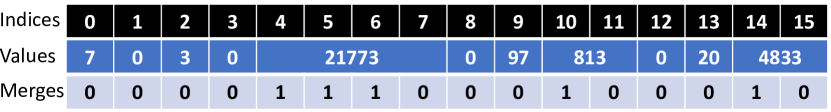
Figure 1: SALSA encoding for an array with a basic counter size of $s=8$ bits, notice that large counters consume more indices than small counters due to merge operations.

Reducing the Encoding Overhead: The encoding we used in SALSA so far is efficient as well as amenable for simple implementation. The cost of this encoding is a single merge bit per counter. This is, in fact, within a factor of 2 of the optimal encoding, as we show in Appendix A. That is, we prove that any encoding for SALSA must use at least $\log_{2}1.5\approx 0.585$ overhead bits per counter and show a somewhat more complex $O(1)$-time encoding with at most $0.594$ overhead bits per counter. For a given memory allocation, this encoding provides improved accuracy as the lower overhead allows fitting more counters, but may be somewhat slower.

Fine-grained Counter Merges: The SALSA encoding we presented in Section IV doubles the counter size upon an overflow, which may be wasteful when the overflowing counter could benefit from a smaller increase in size. Thus, we suggest the more refined Tango algorithms to explore the benefits of a more fine-grained merging strategy. In Tango, counters can be merged into sizes that are arbitrary multiples of $s$. For example, if we start from $s=8$ bit counters, Tango can merge a $16$ bit counter into a $24$ bit counter while SALSA would merge from $16$ bits to $32$. The encoding of Tango is simple: each counter $j$ is associated with a merge bit $m_{j}$ that denotes whether the counter is merged with its right-neighbor. To compute the counter size and offset in Tango of $j=h(x)$, we scan the number of set bits to the left and right of $m_{j}$ until we hit a zero at both sides. For example, if $j=5$ and $m_{4}=m_{5}=m_{6}=m_{7}=1$ while $m_{3}=m_{8}=0$ then the counter consists of $s\cdot 5$ bits, spanning $\left\langle 4,5,6,7,8\right\rangle$. In general, one can use complex logic to decide whether to merge with the left or right neighbor once a counter overflows. However, we design Tango to evaluate the potential benefits of fine-grained merging and therefore enforce a merging logic that mimics SALSA. Specifically, Tango always tries to be aligned to the smallest possible power of two. For example, if counter $9$ overflows, it merges with $8$ to be aligned with the $2$-block $\left\langle 8,9\right\rangle$. If it overflows again, it merges with $10$ (creating a $s\cdot 3$ bits sized counter) and then with $11$. If more bits are needed it will merge with $12$ then with $13,14$ and $15$ (being aligned to the $8$-block $\left\langle 8,\ldots,15\right\rangle$). Then it merges with $7,6,\ldots$, etc. Notice that at every point in time, the Tango counters are contained in the corresponding SALSA counters. In particular, this allows us to produce an estimate that is at least as accurate as SALSA. We note that Tango poses a tradeoff – while it allows more accurate sketches (e.g., as a counter may not exceed $2^{24}-1$ and thus it could be wasteful to merge it into $32$ bits), it also has slower decoding time and cannot use the efficient encoding of the previous section.

V SALSA-fying Sketches

We now describe how SALSA integrates with existing sketches, and specifically how to set the value of merged counters in each sketch. We also state and prove accuracy guarantees for the resulting SALSA sketches. We employ hash functions $h_{i}:U\to[w]$ similarly to the original sketches. Given a merged counter with indices $\left\langle L,L+1,\ldots,R\right\rangle$, we consider all elements $x$ with $L\leq h_{i}(x)\leq R$ to be mapped into it. Hereafter, we often refer to the underlying sketch as following: If the largest merged counter size is $s\cdot 2^{\ell}$, the underlying sketch is a vanilla (fixed counter size) sketch where each counter is of size $s\cdot 2^{\ell}$ and its hashes are $\left\{\widetilde{h}_{i}(x)\triangleq\left\lfloor{h_{i}(x)/2^{\ell}}\right\rfloor\mid i\in[d]\right\}$.

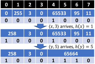
(a) Sum merging of counters

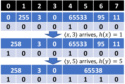
(b) Max merging of counters

Figure 2: Sum and Max merge in SALSA CMS with $s=8$.

Count Min Sketch (CMS): SALSA CMS and Tango CMS are identical to CMS as long as no counter overflows. We have already defined the merge operation with regard to encoding (Section IV), and with regard to hash mapping in the previous section. However, we still need to define how we determine the value of a merged counter, which provides a degree of freedom we leverage to increase measurement accuracy according to the specific model requirements. A natural merging operation is to sum the merged counter values (illustrated in Figure 2a). We formalize the correctness of this approach for the Strict Turnstile model via the following theorem.

Theorem V.1.

Assume that SALSA and Tango use sum merge to unify counters. Let $2^{\ell}\cdot s$ be the maximal bit-size of any counter in SALSA CMS, and $\forall i\in[d]$ let $\widetilde{h}_{i}(x)=\left\lfloor{h_{i}(x)/2^{\ell}}\right\rfloor$ be hash functions that map items into a standard CMS with $(2^{\ell}\cdot s)$-sized counters. Then for any $x\in U:f_{x}\leq\widehat{f_{x}^{\text{Tango}}}\leq\widehat{f_{x}^{\text{SALSA}}}\leq\widehat{f_{x}^{\text{CMS}}}$, where $\widehat{f_{x}^{\text{Tango}}},\widehat{f_{x}^{\text{SALSA}}}$ and $\widehat{f_{x}^{\text{CMS}}}$ are the estimates of Tango, SALSA, and the underlying CMS (with functions $\widetilde{h}_{i}(x)$).

Proof.

The sum merge maintains an invariant where the value of each merged counter is the total frequency of all elements mapped to it. In the worst case, a merge results in a counter of size equal to that of the corresponding counter in the underlying CMS. In this case, the values of the counters are identical. Otherwise, the value of a Tango counter is upper bounded by a SALSA counter which, in turn, is upper bounded by the corresponding value in the underlying CMS. ∎

For Cash Register streams (with only positive updates), rather than sum the counters when merging, we can take the maximum value of the merged counters to gain more accuracy (exemplified in Figure 2b) while maintaining guarantees, as formalized in the following theorem.

Theorem V.2.

Assume that SALSA and Tango use max merge to unify counters. Let $2^{\ell}\cdot s$ be the maximal bit-size of any counter in SALSA CMS, and $\forall i\in[d]$ let $\widetilde{h}_{i}(x)=\left\lfloor{h_{i}(x)/2^{\ell}}\right\rfloor$ be hash functions that map items into a standard CMS with $(2^{\ell}\cdot s)$-sized counters. Then for any $x\in U:f_{x}\leq\widehat{f_{x}^{\text{Tango}}}\leq\widehat{f_{x}^{\text{SALSA}}}\leq\widehat{f_{x}^{\text{CMS}}}$, where $\widehat{f_{x}^{\text{Tango}}},\widehat{f_{x}^{\text{SALSA}}}$ and $\widehat{f_{x}^{\text{CMS}}}$ are the estimates of Tango, SALSA, and the underlying CMS (with functions $\widetilde{h}_{i}(x)$).

Proof.

After each merge, the counter value upper bounds the frequency of any element mapped to the hash range of the merged counter. In addition, the value of SALSA and Tango counters when using the max merge are upper bounded by the corresponding value of SALSA and Tango counters when using the sum merge. ∎

Theorems V.1 and V.2 show that SALSA CMS and Tango CMS are at least as accurate as the underlying CMS for both merge operations. Intuitively, by sum-merging every consecutive $\overline{n}$ bits, we obtain estimates that are identical to a CMS sketch that uses $\overline{n}$ bit counters. Therefore, sum-merging SALSA’s estimates are upper bounded by the CMS estimates. In Cash Register streams, max-merging estimates are upper bounded by the sum-merging ones. Finally, for any given element, the estimates of SALSA CMS and Tango CMS are lower bounded by its true frequency, which implies that our approach provides the same error guarantee as the underlying sketch.

SALSA CMS also improves the performance of count distinct queries for Linear Counting [37] using CMS. Recall Linear Counting estimates the number of distinct queries using the fraction $p$ of zero counters. We consider running Linear Counting using SALSA CMS staring with $s=8$ bit counters, compared to a standard CMS implementation using 32-bit counters. Unlike standard CMS, SALSA may be unable to determine the exact number of ($s$-bit) counters that remain zero, as some are merged into other counters. Instead, we compute the fraction $\mathfrak{f}$ of $s$-bit counters that remained zero from the overall number of counters that did not merge. For every counter that is the result of one or more merges, we know that at least one of its sub-counters is not zero; we optimistically assume that a fraction $\mathfrak{f}$ of its remaining sub-counters are zero. So, for example, our estimate of the number of counters that are 0 is the number of $s$-bit counters that remained zero, plus $\mathfrak{f}$ times the number of $2s$-bit counters, plus $3\mathfrak{f}$ times the number of $4s$-bit counters, and so on if there are larger counters. Note that this approach is heuristic and its accuracy guarantees are left as future work.

Conservative Update Sketch (CUS): SALSA CUS is similar to the standard CUS – whenever an update $\left\langle x,v\right\rangle$ arrives, each counter $C[i,h_{i}(x)]$ is set to $\max\left\{C[i,h_{i}(x)],v+\widehat{f_{x}}\right\}$ with $\widehat{f_{x}}=\min_{i\in[d]}C[i,h_{i}(x)]$ being the previous frequency estimate for $x$. Unlike the CMS variant, the correctness of SALSA CUS is not immediate as not all counters are increased for each packet. Theorem V.3 shows that SALSA CUS is correct in the Cash Register model when working with the max-merge method.

Theorem V.3.

Let $2^{\ell}\cdot s$ be the maximal bit-size of any counter in max-merge SALSA CUS, and $\forall i\in[d]$ let $\widetilde{h}_{i}(x)=\left\lfloor{h_{i}(x)/2^{\ell}}\right\rfloor$ be hash functions that map items into a standard CUS with $(2^{\ell}\cdot s)$-sized counters. Then for any $x\in U:f_{x}\leq\widehat{f_{x}^{\text{SALSA}}}\leq\widehat{f_{x}^{\text{CUS}}}$, where $\widehat{f_{x}^{\text{SALSA}}}$ and $\widehat{f_{x}^{\text{CUS}}}$ are the estimates of SALSA and the underlying CUS (with functions $\widetilde{h}_{i}(x)$).

Proof.

It is sufficient to consider only updates with $v=1$ since each $\left\langle x,v\right\rangle$ update is identical to $v$ consecutive $\left\langle x,1\right\rangle$ updates. The proof is by induction on the number of updates. Specifically, we show that after each update it holds that

$$\forall x,i\in[d]:C_{SALSA}[i,h_{i}(x)]\leq C_{CUS}[i,\tilde{h}_{i}(x)]\ ,$$ (2)

where we denote by $C_{SALSA}$ and $C_{CUS}$ the counters of SALSA and the underlying CUS, respectively.

As a base case, initially $C_{SALSA}[i,h_{i}(x)]=C_{CUS}[i,\tilde{h}_{i}(x)]=0\,\,\forall i\in[d]$. We show that if Equation (2) holds, it continues to hold after an additional update.

Case 1: $C_{SALSA}[i,h_{i}(x)]=C_{CUS}[i,\tilde{h}_{i}(x)]$. In this case, on update $\left\langle x,1\right\rangle$, $C_{CUS}[i,\tilde{h}_{i}(x)]$ is increased by CUS. Therefore the claim trivially holds if there is no overflow in SALSA. If there is an overflow, the claim holds by the virtue of the max-merge. That is, the value of the merged counter grows by exactly 1. This also means that the inequality holds for all counters involved in this merge since they are all upper bounded by $C_{CUS}[i,h_{i}(x)]$ prior to the update.

Case 2: $C_{SALSA}[i,h_{i}(x)]<C_{CUS}[i,\tilde{h}_{i}(x)]$. In this case, on update $\left\langle x,1\right\rangle$, the claim trivially holds if there is no overflow in SALSA. If there is an overflow, by the virtue of the max-merge, the value of the merged counter still only grows by 1. This also means that the inequality holds for all counters involved in this merge since they are all upper bounded by $C_{CUS}[i,h_{i}(x)]$ prior to the update, and therefore are upper bounded by $C_{CUS}[i,\tilde{h}_{i}(x)]$ after it. ∎

Count Sketch (CS): SALSA can also extend the CS, with a minor modification. Unlike most existing implementations, which use the standard Two’s Complement encoding, SALSA CS uses a sign-magnitude representation of counters (as counters can be negative), with the most significant bit for the sign and the rest as magnitude. While Two’s Complement represents values in the range $\left\{-2^{s-1},\ldots,2^{s-1}-1\right\}$, sign-magnitude does not allow a representation of $-2^{s-1}$. However, our use of sign-magnitude is critical for us to ensure that the overflow event is sign-symmetric, which allow us to prove that our sketch is unbiased. When an $s\cdot 2^{\ell}$ bits counter exceeds an absolute value of $2^{s\cdot 2^{\ell}-1}-1$, we merge to double its size. When merging counters in SALSA CS, we use sum-merge; note max-merge may not be correct as counters may have opposite signs. We prove the correctness of SALSA CS. For simplicity, we focus on the main variant. That is, a counter merges at most twice, starting from $s=8$ bits and assuming that no counter reaches an absolute value of $2^{31}$, which is the common implementation assumption.

Let $x\in U$ be an element mapped to counter $A$, which may be merged with counter $B$ to create $\left\langle A,B\right\rangle$, which in turn may later merge with $\left\langle C,D\right\rangle$ to make the $4s$-bit counter $\left\langle A,B,C,D\right\rangle$. This setting is illustrated to the right:

We wish to show that the estimates of each row in SALSA CS are unbiased, and further that each estimate has variance with SALSA CS that is no larger than the corresponding variance with CS. As mentioned, here give a full analysis for starting with $s$ bit counters and allowing counters to grow to $4s$ bits, as this is the focus in our implementation, but the approach generalizes readily to additional levels. we now introduce some notation to analyze SALSA CS.

We use $O_{AB}$ to denote the event that $A$ and $B$ have been merged at query time (either into $\left\langle A,B,C,D\right\rangle$ or just as $\left\langle A,B\right\rangle$) and $O_{ABCD}$ for the event that $A,B,C,$ and $D$ have been merged into $\left\langle A,B,C,D\right\rangle$. We also denote the value of $A$ by (the random variable) $X_{A}$, the value of $\left\langle A,B\right\rangle$ by $X_{AB}$, and similarly for $X_{B}$, $X_{CD}$, and $X_{ABCD}$. We emphasize that $X_{S}$ represents the value of the count mapped to $S$, regardless of whether the counter overflows (e.g., $X_{A}\triangleq\sum_{y\in U:h(y)=A}f_{y}g(y)$ even if $X_{A}\geq 2^{s}$). Without loss of generality, we also assume that the sign of $x$ is $g(x)=1$ (and thus $\mathbb{E}[X_{A}]=\mathbb{E}[X_{AB}]=\mathbb{E}[X_{ABCD}]=f_{x}$). This allows us to express the estimate given in a row for SALSA CS as: $\widehat{f_{x}}=X_{A}(1-O_{AB})+X_{AB}\cdot O_{AB}\cdot(1-O_{ABCD})+X_{ABCD}\cdot O_{ABCD}=X_{A}(1-O_{AB})+X_{AB}\cdot O_{AB}-X_{AB}\cdot O_{AB}\cdot O_{ABCD}+X_{ABCD}\cdot O_{ABCD}.$ Observe that $O_{ABCD}\subseteq O_{AB}$ and thus $O_{AB}\cdot O_{ABCD}=O_{ABCD}$. This implies that (since $X_{AB}-X_{A}=X_{B}$ and $X_{ABCD}-X_{AB}=X_{CD}$):

$$\widehat{f_{x}}=X_{A}+X_{B}\cdot O_{AB}+X_{CD}\cdot O_{ABCD}.$$ (3)

We continue by proving that the estimate is unbiased.

Lemma V.4.

SALSA is unbiased, i.e., $\mathbb{E}[\widehat{f_{x}}]=f_{x}.$

Proof.

Due to the sign-symmetry of the sign function $g$, we have that $\mathbb{E}[X_{B}|O_{AB}]=0$ and $\mathbb{E}[X_{CD}|O_{ABCD}]=0$ (as $\forall\mathfrak{i}:\Pr[X_{B}=\mathfrak{i}|O_{AB}]=\Pr[X_{B}=-\mathfrak{i}|O_{AB}]$ and $\Pr[X_{CD}=\mathfrak{i}|O_{ABCD}]=\Pr[X_{CD}=-\mathfrak{i}|O_{ABCD}]$). Thus, according to (3):

$$\mathbb{E}[\widehat{f_{x}}]=\mathbb{E}\left[X_{A}+X_{B}O_{AB}+X_{CD}O_{ABCD}\right]=\mathbb{E}\left[X_{A}\right]\\ +\mathbb{E}\left[X_{B}|O_{AB}\right]\Pr[O_{AB}]+\mathbb{E}\left[X_{CD}|O_{ABCD}\right]\Pr[O_{ABCD}]=f_{x}.\qed$$

We show that SALSA reduces the variance in each row.

Lemma V.5.

$\mathrm{Var}[\widehat{f_{x}}]\leq\mathrm{Var}[CS],$ where $\mathrm{Var}[CS]\triangleq\mathrm{Var}[X_{ABCD}]$ is the variance of the underlying Count Sketch.

Proof.

Let us prove that $\mathrm{Var}[CS]-\mathrm{Var}[\widehat{f_{x}}]\geq 0$. Observe that since CS and SALSA CS are unbiased, we have that:

$$\mathrm{Var}[ CS]-\mathrm{Var}[\widehat{f_{x}}]$$

$$=\mathbb{E}\left[\left({X_{ABCD}-f_{x}}\right)^{2}\right]-\mathbb{E}\left[\left({\widehat{f_{x}}-f_{x}}\right)^{2}\right]$$

$$=\mathbb{E}\left[{X_{ABCD}^{2}-\widehat{f_{x}}^{2}-2f_{x}X_{ABCD}+2f_{x}\widehat{f_{x}}}\right]$$

$$=\mathbb{E}\left[X_{ABCD}^{2}\right]-\mathbb{E}\left[\widehat{f_{x}}^{2}\right]+2f_{x}\mathbb{E}\left[\widehat{f_{x}}-X_{ABCD}\right].$$

Due to unbiasedness, $\mathbb{E}\left[\widehat{f_{x}}\right]=\mathbb{E}\left[X_{ABCD}\right]=f_{x}$ and thus

$$\mathrm{Var}[CS]-\mathrm{Var}[\widehat{f_{x}}]=\mathbb{E}\left[X_{ABCD}^{2}\right]-\mathbb{E}\left[\widehat{f_{x}}^{2}\right].$$ (4)

We continue by simplifying the expression for $\mathbb{E}\left[\widehat{f_{x}}^{2}\right]$:

$$\mathbb{E} \left[\widehat{f_{x}}^{2}\right]=\mathbb{E}\left[\left({X_{A}+X_{B}O_{AB}+X_{CD}O_{ABCD}}\right)^{2}\right]$$

$$=\mathbb{E}\left[X_{A}^{2}\right]+\mathbb{E}\left[X_{B}^{2}O_{AB}\right]+\mathbb{E}\left[X_{CD}^{2}O_{ABCD}\right]$$

$$+2\Bigg{(}\mathbb{E}\left[X_{A}X_{B}O_{AB}\right]+\mathbb{E}\left[X_{A}X_{CD}O_{ABCD}\right]$$

$$\qquad+\mathbb{E}\left[X_{B}X_{CD}O_{ABCD}\right]\Bigg{)}$$

$$=\mathbb{E}\left[X_{A}^{2}\right]+\mathbb{E}\left[X_{B}^{2}|O_{AB}\right]\Pr[O_{AB}]$$

$$+\mathbb{E}\left[X_{CD}^{2}|O_{ABCD}\right]\Pr[O_{ABCD}]+2\Big{(}\mathbb{E}\left[X_{A}X_{B}|O_{AB}\right]\Pr[O_{AB}]$$

$$+\mathbb{E}\left[X_{A}X_{CD}|O_{ABCD}\right]\Pr[O_{ABCD}]$$

$$+\mathbb{E}\left[X_{B}X_{CD}|O_{ABCD}\right]\Pr[O_{ABCD}]\Big{)}.$$

Since $x$ is mapped to $A$, we can use the sign-symmetry of $X_{B}$ and $X_{CD}$ to get $\mathbb{E}\left[X_{A}X_{B}|O_{AB}\right]=\mathbb{E}\left[X_{A}X_{CD}|O_{ABCD}\right]=\mathbb{E}\left[X_{B}X_{CD}|O_{ABCD}\right]=0$, which gives

$$\mathbb{E}\left[\widehat{f_{x}}^{2}\right]=\mathbb{E}\left[X_{A}^{2}\right]+\mathbb{E}\left[X_{B}^{2}|O_{AB}\right]\Pr[O_{AB}]\\ +\mathbb{E}\left[X_{CD}^{2}|O_{ABCD}\right]\Pr[O_{ABCD}]=\mathbb{E}\left[X_{A}^{2}\right]+\mathbb{E}\left[X_{B}^{2}\right]+\mathbb{E}\left[X_{CD}^{2}\right]\\ -\left({\mathbb{E}\left[X_{B}^{2}|\neg O_{AB}\right]\Pr[\neg O_{AB}]+\mathbb{E}\left[X_{CD}^{2}|\neg O_{ABCD}\right]\Pr[\neg O_{ABCD}]}\right)\\ \leq\mathbb{E}\left[X_{A}^{2}\right]+\mathbb{E}\left[X_{B}^{2}\right]+\mathbb{E}\left[X_{CD}^{2}\right].$$ (5)

Now, notice that $X_{ABCD}^{2}=\left({X_{A}+X_{B}+X_{CD}}\right)^{2}=X_{A}^{2}+X_{B}^{2}+X_{CD}^{2}+2(X_{A}X_{B}+X_{A}X_{CD}+X_{B}X_{CD})$. Due to the sign-symmetry of $g$, we have $\mathbb{E}\left[X_{A}X_{B}\right]=\mathbb{E}\left[X_{A}X_{CD}\right]=\mathbb{E}\left[X_{B}X_{CD}\right]=0$ and thus: $\mathbb{E}\left[X_{ABCD}^{2}\right]=\mathbb{E}\left[X_{A}^{2}\right]+\mathbb{E}\left[X_{B}^{2}\right]+\mathbb{E}\left[X_{CD}^{2}\right]\geq\mathbb{E}\left[\widehat{f_{x}}^{2}\right],$ where the inequality follows from (5). Together with (4), this concludes the proof. ∎

Because the theorem shows the error variance is no larger for each row, following the same analysis as for CS (using Chebyshev’s inequality to bound the error of the row and then Chernoff’s inequality to bound the error of the median) yields the same error bounds for SALSA CS. Indeed, we expect better estimates using SALSA as the inequality from the proof of the theorem ($\mathrm{Var}[CS]\geq\mathrm{Var}[\widehat{f_{x}}]$) is usually a strict inequality. In our experimental evaluation, we show that SALSA CS obtains better estimates than CS.

Theorem V.6.

Let $2^{\ell}\cdot s$ be the maximal bit-size of any counter in sum-merge SALSA CS, and $\forall i\in[d]$ let $\widetilde{h}_{i}(x)=\left\lfloor{h_{i}(x)/2^{\ell}}\right\rfloor$ be hash functions that map items into a standard CS with $(2^{\ell}\cdot s)$-sized counters. Then for any $x\in U,i\leq d:\mathbb{E}\left[C_{SALSA}[i,h_{i}(x)]\cdot g_{i}(x)\right]=f_{x}$ and $\mathrm{Var}\left[C_{SALSA}[i,h_{i}(x)]\cdot g_{i}(x)-f_{x}\right]\leq\mathrm{Var}\left[C_{CS}[i,\tilde{h}_{i}(x)]\cdot g_{i}(x)-f_{x}\right]$, where $C_{SALSA}[i,h_{i}(x)]$ and $C_{CS}[i,\tilde{h}_{i}(x)]$ are the counters of SALSA and the underlying CS (with functions $\widetilde{h}_{i}(x)$).

We note that SALSA CS can also provide other derived results, similarly to CS. For example, by using a heap, we can find the $L_{2}$-heavy hitters in Cash Register streams similarly to the original version.

Universal Sketch (UnivMon): The universal monitoring sketch (UnivMon) uses several $L_{2}$ sketches that are applied on different subsets of the universe. By improving the accuracy of CS, we can also improve the performance of UnivMon. We note that since SALSA CS provides an accuracy guarantee that is at least as good as the underlying sketch, SALSA Univmon provides the same accuracy guarantee as the vanilla Univmon.

Merging and Subtracting SALSA Sketches: Given streams $A,B$ and their sketches $s(A),s(B)$, we may then wish to derive statistics on $A\cup B$ (for example, we can parallelize the sketching of $A$ and $B$ and then merge them), or on $A\setminus B$ (for example, to detect changes in our network traffic compared to the previous epoch). By $A\setminus B$, we refer to computing the frequency difference; e.g., if $x$ appeared twice in $A$ and three times in $B$, its frequency in $A\setminus B$ is -1. Most standard sketches are linear, and can be naturally summed/subtracted counter-wise to obtain a sketches $s(A\cup B)\equiv s(A)+s(B)$ and $s(A\setminus B)\equiv s(A)-s(B)$ if they share the same hash functions, and work in the Turnstile model.

SALSA can also merge and subtract sketches. For merging $s(A)$ and $s(B)$, SALSA traverses the counters and merges them according sum-merging. Specifically, each counter in the merged sketches has a size at least as large as its size in $s(A)$ and its size in $s(B)$. Additionally, when summing or subtracting counters an overflow may occur, triggering another merge to make sure we have enough bits to encode the resulting values. CS, as a Turnstile sketch, also supports general subtracting that is done similarly to merging, while CMS (which works in the Strict Turnstile model) can compute $s(A\setminus B)$ given a guarantee that $B\subseteq A$. These operations are illustrated in Figure 3.

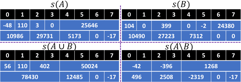
Figure 3: An example of $s=8$ bit SALSA CS merging and subtracting Turnstile sketches $s(A)$ and $s(B)$.

Integrating Estimators into SALSA: Thus far, we have described a single strategy to handle overflows: when a counter reaches a value that can not be represented with the current number of bits, it merges with a neighbor. However, there are alternatives that allow one to increase the counting range. Specifically, estimators can represent large numbers using a smaller number of bits, at the cost of introducing an error.

The state of the art Additive Error Estimators (AEE) [16] offer a simple and efficient technique to increase the counting range. For simplicity, we describe the technique for CMS and unit-weight streams (where all updates are of the form $\left\langle x,1\right\rangle$), although AEE can support weighted updates and other L1 sketches as well. Throughout the execution, incoming updates are sampled with probability $p$. If an update is sampled, it increases the sketch, and otherwise, it is ignored. Whenever a counter overflows, a downsampling event happens. When downsampling, $p$ is halved and any counter $C[i,j]$ is replaced by either $Bin(C[i,j],1/2)$ (called probabilistic downsampling) or by $\left\lfloor{C[i,j]/2}\right\rfloor$ (deterministic downsampling). Since the counter values are reduced as a result of the downsampling, new updates can be processed, and no additional counter bits are needed. For any $\delta_{est}>0$, we have an implied estimation error for AEE given by $\epsilon_{est}\triangleq\sqrt{\frac{2p^{-1}\ln(2/\delta_{est})}{N}}$, such that $\Pr\left[\Big{|}\widehat{C[i,j]}-C[i,j]\Big{|}\geq N\epsilon_{est}\right]=\Pr\Big{[}|\widehat{C[i,j]}-C[i,j]|\geq\sqrt{2Np^{-1}\ln(2/\delta_{est})}\Big{]}\leq\delta_{est}.$ Another motivation for AEE comes from the processing speed. Since the sampling probability is independent of the value of the current counter, one can compute the hash functions $h_{i}(x)$ only if a packet is sampled. Since hash functions are a major bottleneck for sketches [18], AEE is faster than the baseline sketches. Another version of the estimator, called AEE MaxSpeed, aims to maximize the processing speed while bounding the error. Therefore, instead of waiting for a counter to overflow, it downsamples all counters once enough updates have been processed. In comparison with the original variant (called AEE MaxAccuracy), MaxSpeed is faster but less accurate [16].

Intuitively, downsampling and merging increase the error in different ways. While downsampling increases the inherent error of a counter, merging adds noise from other elements that previously have not collided with the counter. SALSA selects how to handle overflows in a way that minimizes the theoretical error increase by either downsampling or merging. Specifically, as our accuracy theorems suggest, the sketch error in SALSA depends on the size of the largest counter. Therefore, unless a largest counter overflows, SALSA opts for merging as its overflow strategy. When a largest counter overflows, SALSA computes the estimator error difference $\Delta_{\mathit{est}}=\sqrt{2}\cdot\epsilon_{est}$, which is the increase in error if we downsample. Similarly, if the currently largest counter is of size $s\cdot 2^{\ell}$, SALSA computes $\epsilon_{CMS}\triangleq\delta^{-1/d}\cdot 2^{\ell}/w$, which is the current accuracy guarantee (see Theorem V.1 and Section III) and $\Delta_{\mathit{CMS}}=\epsilon_{CMS}$ is then the difference in error guarantee that results from merging. We pick $\delta_{est}=\delta/d$ to allow all counters of the current element to be estimated within $\epsilon_{est}$ with probability $1-\delta$. Finally, SALSA chooses to merge if $\Delta_{\mathit{CMS}}\leq\Delta_{\mathit{est}}$, and otherwise it downsamples. As a result, SALSA estimates element sizes to within $N\cdot(\epsilon_{est}+\epsilon_{CMS})$ with a probability of at least $1-2\delta$.

As an optimization, when downsampling, SALSA may be able to split counters if the resulting values can be represented using fewer bits. For example, if $s=8$ and a value of $300$ was represented in the 16-bit counter $\left\langle 4,5\right\rangle$, and if it is then downsampled to a value of $150$, we can split the counter and set both counter $4$ and counter $5$ to $150$. We note that this only works for max-merging, where the accuracy guarantees seamlessly follow.

VI Evaluation

In this section, we extensively evaluate SALSA’s performance on real and synthetic datasets and compare it to that of the underlying sketches. We first document the methodology.

Sketch Configuration Parameters: Unless specified otherwise, all CMS and CUS sketches are configured with $d=4$ rows, as is used e.g., in the Caffeine caching library [38]. Since CS requires taking median over the rows, all CS experiments are configured with $d=5$ rows as done, e.g., in [39]. We configure UnivMon with $16$ CS instances, each configured with $d=5$ and a heap of size $100$, following the implementation of [15]. Such settings are standard for applications that aim for speed rather than being memory-optimal. For the ABC [17] and Pyramid [12] sketches, as well as the Cold Filter [9] framework, we use the configurations recommended by the authors. We pick $s=8$ bit counters as the default configuration of SALSA, motivated by the synthetic results. We use the simple encoding (1 bit of overhead per counter) of Section IV, which uses slightly more space but is faster. The Baseline implementations use 32-bit counters, a choice we justify later in Figure 6, and that is also common in existing implementations [18, 33]. Nonetheless, our SALSA implementation allows counters to grow further, up to $64$ bits. For implementation efficiency, all row widths $w$ are powers of two. When we give figures where an $x$-axis is allocated memory, we include the encoding overheads. For the integration with AEE, we configure SALSA AEE with $\delta=4\cdot\delta_{est}=0.001$ (see Section V).

Datasets: We evaluate our algorithms using four real datasets and several synthetic ones. In particular, we use three network packet traces: two from major backbone routers in the US, denoted NY18 [40] and CH16 [41], and a data center network trace denoted Univ2 [42]. In these traces, we define items using the “5-tuples” of the packets (srcip, dstip, srcport, dstport, proto). Additionally, we use a YouTube video trace [43, US category]. As the video data does not have a recorded order (just view-count), we use a random order where each item is a video independently sampled according to the view-count distribution. Finally, we use random order Zipfian traces. All traces have 98M elements for consistency with the shortest real dataset. In our evaluation, we use unit-weight Cash Register streams (i.e., all updates are of the form $\left\langle x,1\right\rangle$). We also experiment with the task of evaluating change detection, which requires a SALSA sketch under the Turnstile model.

Metrics: For frequency estimates, we use the On-arrival model that asks for an estimate of the size of each arriving element (e.g., [16, 5, 44, 7]). Intuitively, this model is motivated by the need to take per-packet actions in networking, e.g., to restrict the allowed bandwidth to prevent denial of service attacks. Given a stream with $n$ updates, we obtain errors $e_{1},e_{2},\ldots,e_{n}$; the Mean Square Error is defined as $MSE\triangleq n^{-1}\cdot\sum_{i}e_{i}^{2}$, the Root Mean Square Error is then $RMSE\triangleq\sqrt{MSE}$, while the Normalized RMSE is $\mathit{NRMSE}\triangleq n^{-1}\cdot{RMSE}$. Similar metrics are used, e.g., in [16, 44, 7, 5]. Notice that NRMSE is a unitless quantity in the interval $[0,1]$. For fairness, we also evaluate using the error metrics used in Pyramid and ABC: Average Absolute Error (AAE) and Average Relative Error (ARE). AAE averages the error over all the elements with non-zero frequency i.e., $AAE\triangleq\frac{1}{|U_{>0}|}\sum_{x\in U_{>0}}|\widehat{f_{x}}-f_{x}|$, where $U_{>0}\triangleq\left\{x\in U:f_{x}>0\right\}$. Similarly, ARE is defined as $\frac{1}{|U_{>0}|}\sum_{x\in U_{>0}}\frac{|\widehat{f_{x}}-f_{x}|}{f_{x}}$.

For tasks such as Count Distinct, Entropy, and Frequency Moments estimation, we use the Average Relative Error (ARE) metric that averages over the relative error of the ten runs. For turnstile evaluation, we evaluate the capability of SALSA to improve sketches for the Change Detection task (e.g., see [15, 45]) in which we partition the workload into two equal-length parts $A$ and $B$, sketch each, and test the NRMSE of the estimates of the frequency changes between $A$ and $B$. Each data point is the result of ten trials; we report the mean and 95% confidence intervals according to Student’s t-test [46].

Implementation: We leverage existing CMS and CUS implementations from [16] and extend them to implement SALSA. We also extend these to create a Baseline and SALSA implementation of CS. We also used the authors’ code for the Pyramid [12], ABC [17], and Cold Filter [9] algorithms. Particularly, for error measurements, we used the code as-is, while for speed measurements, we applied our optimizations for a fair comparison. All sketches use the same hash functions (BobHash) and index computation methods. When evaluating against the AEE estimators [16], we use the provided open-source code. Similarly, we obtained the UnivMon code from [39] and replaced its CS sketches with SALSA CS to create ’SALSA UnivMon’.

All speed measurements were performed using a single core on a PC with an Intel Core i7-7700 CPU @3.60GHz (256KB L1 cache, 1MB L2 cache, and 8MB L3 cache) and 32GB DDR3 2133MHz RAM.

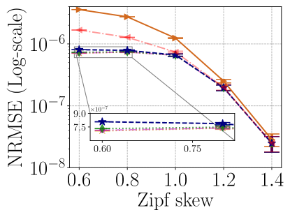
(a) Error, Count Min Sketch (2MB)

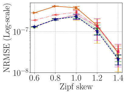
(b) Error, Count Sketch (2.5MB)

Figure 4: Speed and accuracy of SALSA CMS and SALSA CS for the synthetic datasets. The Baseline uses $w=2^{17}$ counters in each row for a total of 2MB of space in CMS and 2.5MB in CS. Here, SALSA_s is using $w=(2^{17}\cdot 32/s)$ sized rows for a total of $2(1+1/s)$MB space for CMS and $2.5(1+1/s)$MB for CS.

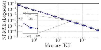
(a) Error, NY18

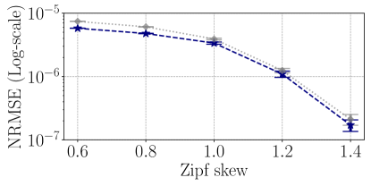
(b) Error, Zipf (2MB)

Figure 5: Accuracy of SALSA CMS with Sum merge vs. Max merge.

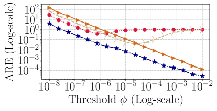
(a) Varying the threshold $\phi$

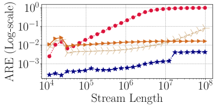
(b) Varying stream length ($\phi=10^{-4})$

Figure 6: SALSA CMS vs. CMS with small counters (2MB).

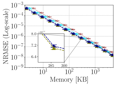
(a) Error, NY18

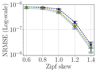
(b) Error, Zipf

Figure 7: Accuracy of SALSA CMS (with $s=8$ bits) vs. Tango CMS. In (b), Tango_s is allocated with $2(1+1/s)$MB of space while SALSA uses $2(1+1/8)=2.25$MB.

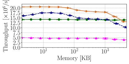
(a) Speed, NY18

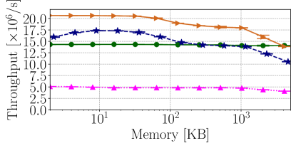
(b) Speed, CH16

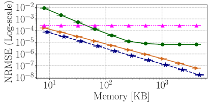
(c) NRMSE Error, NY18

(d) NRMSE Error, CH16

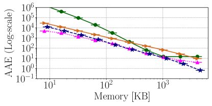
(e) AAE Error, NY18

(f) AAE Error, CH16

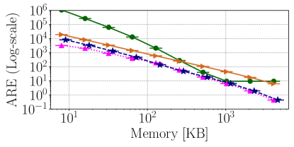
(g) ARE Error, NY18

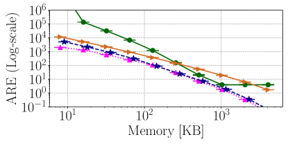
(h) ARE Error, CH16

Figure 8: Comparing the performance of the SALSA, Pyramid [12], ABC [17], and Baseline versions of CMS.

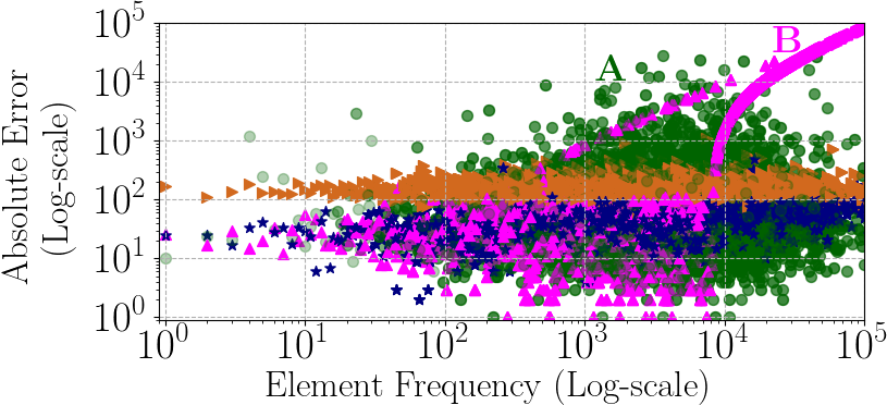
(a) NY18

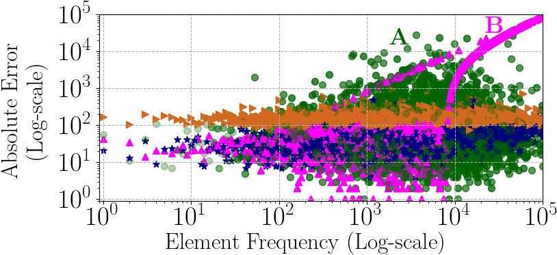
(b) CH16

Figure 9: The error distribution of the algorithms (2MB).

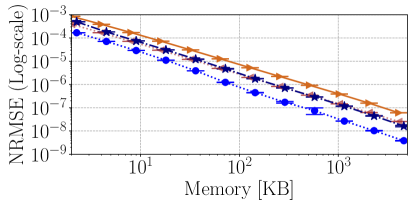
(a) Error, NY18

(b) Error, CH16

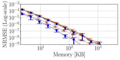
(c) Error, Univ2

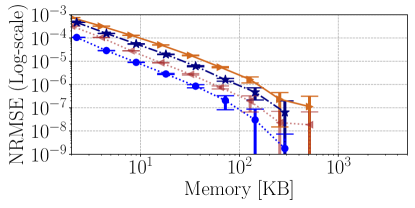
(d) Error, YouTube

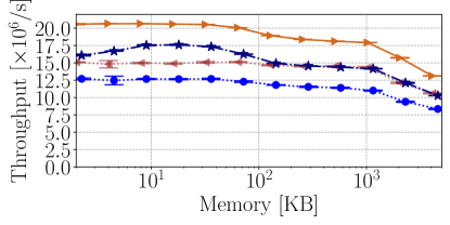
(e) Speed, NY18

(f) Speed, CH16

(g) Speed, Univ2

(h) Speed, YouTube

Figure 10: Speed and accuracy of SALSA CMS and SALSA CUS for the real datasets. Notice the log-scale of the error plots.

How to Configure SALSA? We perform preliminary experiments to determine the default SALSA configuration.

How Large Should Counters Be? We first determine the most effective minimal counter size ($s$) for SALSA. Intuitively, for a fixed row width $w$, smaller $s$ results in lower error but also in larger encoding overheads. With this tradeoff, it may not be profitable to reduce $s$. In this experiment, we fixed the memory of the counters and deliberately ignored the encoding overheads for SALSA. The goal is to quantify the attainable improvement from using smaller counters. We used synthetic Zipfian trace with skews varying from 0.6 to 1.4.

As shown in Figure 4, most of the improvement comes from reducing the counter sizes from $32$ bits to $8$ bits. These results were consistent across different memory footprints. This is not surprising as almost all counters merge up to at least $8$ bits, but then many do not overflow further. We also observe that SALSA offers more gains for low-skew traces and that CS is better suited for lower skews, while CMS offers comparable accuracy with less space for high skew. Hereafter, we use $s=8$ bits as the default SALSA configuration. While SALSA with $s=4$ bits is slightly more accurate for low-skew workloads and high memory footprints, its encoding overhead of about 25% of the sketch size (compared to 12.5% for $s=8$) is too large to justify the benefits.

Which Merging Should We Use? As mentioned above, SALSA CS must use sum-merging, and so does SALSA CMS for Strict Turnstile streams. Similarly, in SALSA CUS, we need to use max-merging. This leaves only the choice for SALSA CMS in Cash Register streams, where we can use either sum-merging or max-merging. We quantify the difference in accuracy in Figure 5. As shown, max-merging is slightly more accurate, especially for low-skew workloads. We conclude that if one only targets Cash Register streams, it is better to use max-merging, but the accuracy of sum-merging is not far behind.

Is Fine-grained Merging Worth It? To understand the accuracy improvement attainable by fine-grained merging (as opposed to SALSA’s approach of doubling the counter size at each overflow), we compare SALSA with Tango. As the results in Figure 7 indicate, Tango also offers the best accuracy-space tradeoff when starting with $s=8$ bits (Tango₁₆ is equivalent to SALSA₁₆ and is omitted). However, while it is slightly more accurate, the gains seem marginal considering the computationally expensive operations of determining the counter’s size and offset. Further, Tango has an overhead of $1$ bit per counter and does not obviously allow an efficient encoding like SALSA does (Section IV).

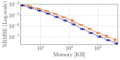
(a) Error, NY18

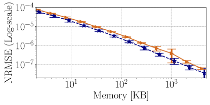
(b) Error, CH16

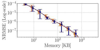
(c) Error, Univ2

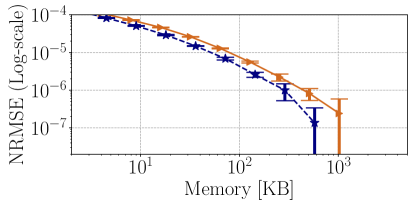
(d) Error, YouTube

Figure 11: Accuracy of SALSA CS for the real datasets.

Can one simply use small counters? In our evaluation, SALSA starts from $s=8$ bit counters. We now compare SALSA with a baseline sketch that uses $8$-bit or $16$-bit counters (as proposed, e.g., in [47]). In such a sketch, the counter is only incremented if it does not overflow (i.e., its value is bounded by $2^{b}-1$ for $b$-bit counters). We show that such solutions cannot capture the sizes of the heavy hitters – elements whose frequency is at least a $\phi$ fraction – which are often considered the most important elements [48]. First, we show (Figure 6a) that when estimating heavy hitters, even with a loose definition of $\phi=10^{-4}$, it is best to use $32$-bit counters for CMS. Similarly, as shown in Figure 6b, when the measurement is longer than 10M elements, the $16$-bit variant becomes less accurate. Figure 6 is depicted for Zipfian trace with skew=1, and we observed similar behavior for other traces, thresholds, and memory footprints.

Comparison with Pyramid Sketch and ABC: We used the authors’ original implementations for both Pyramid Sketch and ABC. We present results for CMS on the NY18 and CH16 datasets; similar results are obtained for additional sketches and workloads.

As shown in Figure 8a, and Figure 8b, Pyramid Sketch and SALSA are about 20% slower than the baseline, while ABC is about 75% slower. Intuitively, the slowdown is expected, as all these algorithms bring additional complexity to the baseline. ABC is significantly slower due is additional encoding overheads as its bit-borrowing technique does not allow byte-alignment for counters, forcing it to make additional bitwise operations for reading and updating counters.

In terms of the NRMSE metric (8c and 8d), SALSA achieves the best results. Next is the baseline following by Pyramid Sketch, and ABC. The on-arrival NRMSE metric gives more weight to the frequent elements, and is more sensitive to larger errors than AAE and ARE. Our results indicate that SALSA is also more accurate than Pyramid Sketch and the baseline in terms of AAE and ARE for the entire memory range. Note that Pyramid Sketch is better than the baseline in the memory range 0.5MB-2MB, which is the range it is optimized for according to the paper. ABC is slightly more accurate than SALSA for small memory sizes but less accurate than SALSA for large memory sizes, and is comparable in between. Our conclusion is that SALSA is the best in the NRMSE metric and is competitive in the AEE, and ARE, and speed metrics.

Understanding the differences: Our first observation, is that the AAE and ARE metrics are not suitable when estimating the size of the heavy hitters, which are often considered the most important elements [48]. This is because both metrics give equal weight to all items, making impact of the error of the largest ones vanish due to averaging. This is evident from Figure 6, in which the leftmost point ($\phi=10^{-8}$) corresponds to the AAE and ARE metrics (as all items are accounted for). As shown, in such a case, using $8$-bit counters yields lower error rates. Nevertheless, such a solution cannot count beyond the value of $255$, which results in excessive error for the heavy hitters (e.g., $\phi=10^{-3}$). In fact, as we show in Appendix B, for CMS, and this dataset, it is better to estimate all sizes as $0$ without performing any measurement. To illustrate the differences that make Pyramid Sketch and ABC competitive in the AAE/ARE metrics, but not in NRMSE, we visualize the errors of estimating individual element frequencies. We sampled one random element from each possible frequency to reduce clutter. The results, showing in Figure 9, demonstrate the differences between the algorithms. SALSA has a low error-variance and is consistently more accurate than the Baseline. In contrast, Pyramid Sketch (as shown in region A) has much higher variance, as elements whose counters overflow share the most significant bits with other elements. ABC, as evident in region B, has a high error on heavy hitters as its counters can at most double in size by combining with their neighbors. We configured ABC to start with $8$-bit counters as suggested by the authors, limiting its estimation to at most $2^{13}-1$ (as three bits are spent on overhead). While one could use larger counters, it would decrease their number and diminish the benefit over the baseline sketch. To conclude, both ABC and Pyramid Sketch have elements with high estimations errors, making them less attractive for (Mean Square Error)-like metrics.

L1 Sketches: We proceed by testing the impact that SALSA (with $s=8$ bit counters) has on the accuracy and speed of L1 sketches, such as CMS and CUS. The results, depicted in Figure 10, show that SALSA CMS is substantially more accurate (roughly requiring half the space for the same error) than the Baseline for the NY18, CH16, and YouTube datasets. For Univ2, SALSA’s improvement is less noticeable, and due to its encoding overheads, the tradeoff is not statistically significant. SALSA CUS is better than the Baseline on all traces, and often requires half the space for a given error.

SALSA’s accuracy comes at the cost of additional operations that are required to maintain the counter layout. We measured SALSA to be 17%-23% slower than the corresponding Baseline variants, but can nonetheless handle 10-17.5 million elements per second on a single core, which is sufficient to support the high link rate forwarding at modern large-scale clusters, such as Google, which is estimated at 9M packets per second (see  [49, Sec. 3.2]) . We note that by combining SALSA with estimators (Section VI), we can make faster counter sketches. We conclude that SALSA offers an appealing accuracy to space tradeoff.

Count Sketch: Next, we evaluate SALSA for Count Sketch, whose L2 guarantee is important for low-skew workloads and more complex algorithms such as UnivMon. As shown in Figure 11, SALSA offers statistically significant improvement for the NY18, CH16, and YouTube datasets. For Univ2, the accuracy improvement is offset by the encoding overhead, and it is not clear which variant is better.

UnivMon: We use SALSA CS to extend the Universal Monitoring (UnivMon) sketch that supports estimating a wide variety of functions of the frequency vector. Our experiment includes estimating the element size entropy and $F_{p}$ moments, for $0\leq p\leq 2$. The result in Figure 12 indicates that SALSA improves the accuracy of both tasks. Interestingly, for entropy estimation, we observe that SALSA’s accuracy (and variance) improve when using smaller ($s=2$ or $s=4$ bit) counters. When using a large amount of memory, SALSA has roughly the same accuracy as the baseline, as both hit a bottleneck in the size of the sketches’ heaps (set to $100$ elements, as in the implementation of [18]).

For estimating $F_{p}$ moments, we measure similar accuracy for small values of $p$ while SALSA improves the accuracy for large $p$ values. To explain this, notice that the element size estimates mainly affect the $F_{p}$ for large $p$, while for $p\approx 0$, the value is determined primarily by the cardinality.

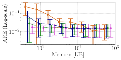
(a) Entropy Estimation

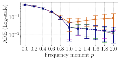
(b) Frequency Moment Estimation (400KB)

Figure 12: Accuracy of SALSA UnivMon for the NY18 dataset.

Cold Filter: We extend Cold Filter by replacing the second-stage CUS (denoted CM-CU in the original paper) algorithm with our SALSA variant. The results in Figure 13 use the AAE and ARE metrics suggested by its authors [9]. The results show that SALSA saves up to 50% of the space for a similar error. However, the improvement is more evident when the allocated memory is small, as in these cases the second stage algorithm plays a significant role. When the memory size is large (compared to the measurement length), the first-stage algorithm handles most of the flows, and improving the second-stage CUS algorithm yields marginal benefits. We observed negligible differences in the processing speed, which is expected as many elements only touch the first stage and do not reach the second. We also tested Cold Filter versus its SALSA variant using the NRMSE metric; there, SALSA yields even larger accuracy gains. However, Cold Filter’s aggregation buffer needs to be drained upon query, which negates its speedup potential in the on-arrival model.

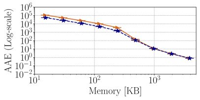
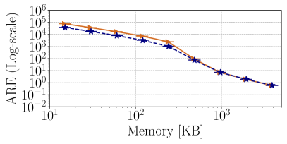
Figure 13: Accuracy of SALSA Cold Filter for the NY18 dataset.

Count Distinct and Heavy Hitters using Count Min: We evaluate the performance of SALSA CMS on additional applications such as counting distinct elements and estimating the size of the heavy hitters. As shown in the count, distinct results (Figures 14(a)-(c)), neither SALSA CMS nor the Baseline are effective with low memory footprints. This is because no counters remain zero-valued, and the Linear Counting estimator fails. Nevertheless, SALSA CMS can work with less memory (4.5MB for NY18 and 1.125MB for CH16) and reduce the estimation error when the Baseline does produce estimates. Intuitively, Linear Counting with $w$ buckets can count up to $w\ln w$ elements, so the number of elements in the datasets (6.5M for NY18 and 2.5M for CH16) imposes a lower bound on the amount of space needed. We evaluate the accuracy for estimating the heavy hitters (elements with frequency of at least $\phi\cdot N$) frequencies, while varying $\phi$ between $10^{-4}$ and $10^{-2}$ as in [48]. SALSA CMS is more accurate, especially for small values of $\phi$. The lower improvement for large $\phi$ values can be explained as $\phi\cdot N\geq 2^{16}$ for $\phi\geq\frac{2^{16}}{98\cdot 10^{6}}\approx 7\cdot 10^{-4}$, which means that all such heavy hitters cause their counters to merge to $32$ bits (the same as the Baseline). The plot of Figure 14d stops around $\phi\approx 3.16\cdot 10^{-4}$ as no element in the NY18 dataset has frequency larger than $5.62\cdot 10^{-4}\cdot N\approx 551K$ packets.

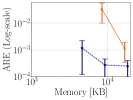
(a) NY18 Dataset

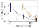
(b) CH16 Dataset

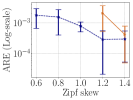
(c) Zipf (8MB)

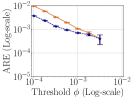
(d) NY18 Dataset

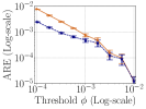
(e) CH16 Dataset

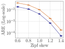
(f) Zipf ($\phi=10^{-4}$)

Figure 14: Accuracy of SALSA CMS on ((a)-(c)) counting distinct elements and ((d)-(f)) estimating the size of heavy hitters with 2MB.

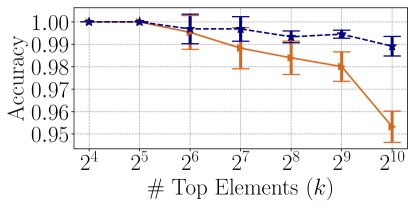
(a) Top-$k$, NY18 (640KB)

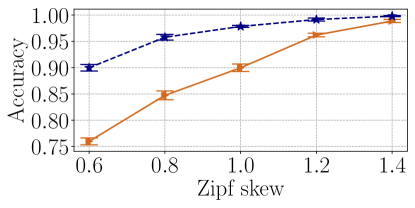
(b) Top-1024, Zipf (640KB)

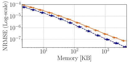
(c) Change Detection, NY18

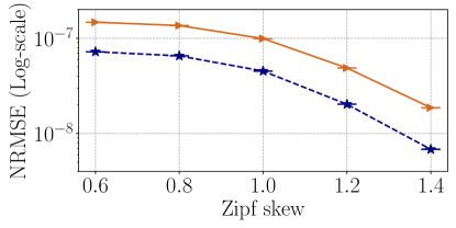
(d) Change Detection, Zipf (2.5MB)

Figure 15: Accuracy of SALSA CS for the Top-$k$ ((a) and (b)) and Change Detection ((c) and (d)) tasks.

Top-$k$ and Change Detection using Count Sketch: We also examine SALSA’s effect on other uses of CS such as Top-$k$ and Change Detection (which requires Turnstile support). For Top-$k$, our experiments indicate that using sufficient memory (e.g., 2MB), the Baseline CS detects the largest elements accurately for reasonable $k$ values. Therefore, we focus on a constrained memory setting (640KB). As shown in Figure 15 (a) and (b), SALSA detects the top-$k$ accurately, especially for large values of $k$ and low-skew workloads.

We also evaluate SALSA CS on a Change Detection task. Here, we split the input into two equal-length intervals $A$ and $B$, the algorithm needs to estimate the change in the frequency of an element $x$ between the first and second halves. To that end, we create sketches $s(A)$ and $s(B)$ and the difference sketch $s(A\setminus B)$ as described in Section V. Intuitively, the frequency difference can be small compared with the frequencies of each interval, and thus directly subtracting the estimates of $s(A)$ and $s(B)$ could yield a poor result compared to taking the difference sketch (as the desired error is a fraction of the $L_{2}$ norm of the frequency difference). In Figure 15 (c) and (d), we compute the NRMSE error over the set of elements that appear in either $A$ or $B$. As shown, SALSA provides a statistically significant accuracy improvement in all tested memory allocations and dataset skews.

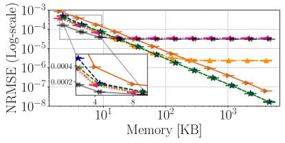
(a) Error, NY18

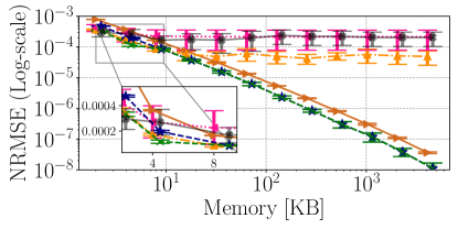
(b) Error, CH16

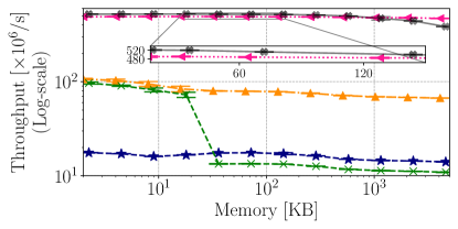
(c) Speed, NY18

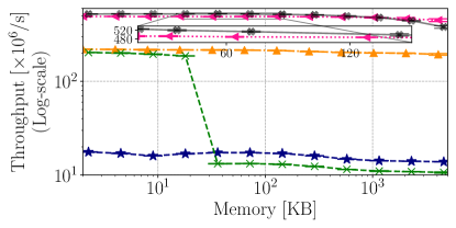
(d) Speed, CH16

Figure 16: Comparison with Estimator Algorithms (CM sketch).

Estimators: We now experiment with integrating estimators, specifically AEE  [16], into SALSA CMS. Under certain conditions, AEE increases the accuracy and processing speed of the sketch. Intuitively, the accuracy can be increased as the sketch can use more estimators than it would use counters, and the speed is increased because some packets are ignored without updating the estimators. Our estimator-integrated solution SALSA AEE (from Section V) optimizes the accuracy by interleaving estimator downsampling and estimator merges. Roughly speaking, SALSA AEE aims to be at least as accurate as the best of SALSA CMS and AEE MaxAccuracy by choosing the best method to cope with each overflow. Similarly to AEE MaxSpeed, we create a speed-optimized variant called SALSA AEE_d that downsamples on the first ${\mathfrak{d}}$ overflows (and selects whether to merge or downsamples afterward according to the logic presented in Section V). This allows the algorithm to reach a sampling rate of $2^{-\mathfrak{d}}$ and thus obtain speedups by reducing hash computations.

The results, shown in Figure 16, illustrate that SALSA AEE is always as accurate as SALSA (when SALSA only merges counters), and more accurate for small amounts of memory. For large amounts of memory, SALSA AEE only merges, and therefore its accuracy is identical to SALSA while it is slightly slower due to the added logic. Compared with AEE MaxAccuracy, SALSA AEE has comparable accuracy for small memory allocations (where it is mostly better to downsample than merge). Further, for large memory allocations (e.g., 100KB or higher), SALSA AEE is more accurate than AEE MaxAccuracy, as in such scenarios it is better to merge than to downsample. Compared with AEE MaxSpeed, SALSA AEE₁₀ provides improved accuracy (by up to 25%), especially for small amounts of memory, while also being faster (by up to 7%), except when using large space (2MB+ in this experiment).

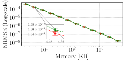
(a) Error, NY18

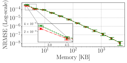
(b) Error, CH16

Figure 17: Affect of splitting counters in SALSA AEE (CM sketch).

Should We Split Counters? Finally, we check the accuracy gains obtainable by splitting counters. Intuitively, once a counter is downsampled, it may require fewer bits to represent. Therefore, if previously the counter had $s\cdot 2^{\ell}$ bits and the downsampled value is lower than $2^{s\cdot 2^{\ell-1}}-1$ (and $\ell\geq 1$), we can split the counter into two $s\cdot 2^{\ell-1}$-bit counters. As a result, there are now fewer collisions between elements, and SALSA AEE has better accuracy. However, as the results in Figure 17 suggest, this effect is minor, and in most cases, the accuracy gains are insignificant.

VII Conclusions

We have presented SALSA, an efficient framework for dynamically re-sizing counters in sketching algorithms, extending counters only when needed to represent larger numbers. SALSA starts from small counters and gradually adapts its memory layout to optimize the space-accuracy tradeoff. By evaluating across multiple real-world traces, sketches, and tasks, we have shown that, for a small overhead for its merging logic, SALSA reduces considerably the measurement error. In particular, our evaluation indicates that SALSA improves on state-of-the-art solutions such as Pyramid Sketch [12], ABC [17], Cold Filter [9], and the AEE estimators [16].

We believe that SALSA can replace and enhance existing sketches in more complex algorithms, such as $L_{p}$-samplers [50] and database systems (e.g., [51, 52]). All of our code is released as open source [1].

Appendix A Improved Encoding

Here, we lower bound the space required to encode SALSA, and then suggest a near-optimal encoding that has $O(1)$ time operations.

Lower bound. For $n\in\mathbb{N}$, we define by $a_{n}$ the number of possible layouts for a consecutive block of $2^{n}\cdot s$ bits (i.e., a block that started from $2^{n}$ counters of size $s$-bits each). For example, we have $a_{2}=5$ since the possible combinations for $4$ consecutive counters are $\left\langle\left\{a\right\},\left\{b\right\},\left\{c\right\},\left\{d\right\}\right\rangle,\left\langle\left\{a,b\right\},\left\{c\right\},\left\{d\right\}\right\rangle,\left\langle\left\{a\right\},\left\{b\right\},\left\{c,d\right\}\right\rangle,\allowbreak\left\langle\left\{a,b\right\},\left\{c,d\right\}\right\rangle,\left\langle\left\{a,b,c,d\right\}\right\rangle.$ Observe that either all $2^{n}$ counters are merged together, or it is enough to specify the layouts of the first $2^{n-1}$ counters and last $2^{n-1}$ counters. Therefore, we get the recursive relation $a_{n}=a_{n-1}^{2}+1$ and $a_{0}=1$. Given that we start from $w$ counters, this implies that the number of possible layouts is lower bounded by $a_{\left\lfloor{\log_{2}w}\right\rfloor}.$

Lemma A.1.

$\forall n\in\mathbb{N}:\left\lfloor{1.5^{2^{n}}}\right\rfloor\leq a_{n}<1.51^{2^{n}}$.

Proof.

The inequality is easy to verify for $n\leq 3$. By induction, one can then easily prove that $\forall n\geq 3:1.5^{2^{n}}+1<a_{n}<1.51^{2^{n}}-1.$ ∎

This suggests a lower bound of $\left\lceil{\log_{2}a_{\left\lfloor{\log_{2}w}\right\rfloor}}\right\rceil\leq\left\lceil{2^{\left\lfloor{\log_{2}w}\right\rfloor}\log_{2}1.5}\right\rceil$ bits. Specifically, for $w\geq 2^{4}$ values which are powers of $2$ any encoding must use at least $\log_{2}1.5\approx 0.585$ bits per counter.

Near-optimal encoding. Denote by $\mathfrak{m}$ the maximal number of merges a single counter may go through during the execution. We note that $\mathfrak{m}=O(1)$ as we assumed the final counters must fit into $O(1)$ machine words. For example, if we start from $s=2$ bits counters and we assume that counters grow up to $128$ bits, then $\mathfrak{m}=6$. Let $\overline{m}=\max\left\{5,\mathfrak{m}\right\}$. Intuitively, we encode every $2^{\overline{m}}$ counters separately, thereby allowing $O(\overline{m})=O(1)$ time size computation. According to Lemma A.1, we have that $z_{\overline{m}}\triangleq\left\lceil{\log_{2}a_{\overline{m}}}\right\rceil$ bits are enough to encode the counter-set layout; for example, $z_{5}=19$ bits are enough to encode the layout of $2^{5}=32$ counters. Specifically, for $n=\overline{m},\overline{m}-1,\ldots,0$ we write a $z_{n}$-bits value $X_{n}$ such that $X_{n}=a_{n}-1$ means that all $2^{n}$ counters are encoded, and otherwise $X_{n-1}\triangleq\left\lfloor{X_{n}/a_{n-1}}\right\rfloor$ encodes the layout of the first $2^{n-1}$ counters while $X_{n-1}^{\prime}\triangleq X_{n}\mod a_{n-1}$ encodes the layout of the rest (i.e., they are the base-$(a_{n-1})$ digits of $X_{n}$). As a result, we use $z_{\overline{m}}$ bits for each consecutive set of $2^{\overline{m}}$ counters, giving an overhead of $z_{\overline{m}}/2^{\overline{m}}$. For $n\geq 5$, we have that $z_{n}/2^{n}<0.594$, i.e., we require at most $0.594$ overhead bits per counter. Computing the size of a counter then becomes simple: we start from $n=\overline{m}$ and every time check if the value is $a_{n}-1$, or recurse into either the left or right half depending on the counter index. An example of this process is illustrated in Figure 18. While this approach reduces the overhead, the decoding process involves division and modulo operations that may reduce the speed.

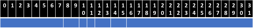
Figure 18: An encoding example for $\overline{m}=5$. This layout is encoded by $X_{5}=449527<a_{5}$. To compute the size of counter $9$, we first check that $X_{5}<a_{5}-1$ and thus not all counters are merged. Next, we have that $X_{4}=\left\lfloor{X_{5}/a_{4}}\right\rfloor=663<a_{4}-1$ and thus counters 0-15 are not all merged. Then, we check that $X_{3}^{\prime}=X_{4}\mod a_{3}=13<a_{3}-1$ which means that counters 8-15 are not all merged. We continue with $X_{2}=\left\lfloor{X_{3}^{\prime}/a_{2}}\right\rfloor=2<a_{2}-1$ (thus 8-11 are not merged) and finally get $X_{1}=\left\lfloor{X_{2}/a_{1}}\right\rfloor=1=a_{1}-1$ which implies that $9$ is merged with $8$.

Appendix B Understanding the Differences – Extended Results

For completeness, we repeat the experiment in Figure 6 using even smaller ($4$-bit) counters. The results are shown in figures 19 and 20. We measured the error on all heavy hitters – elements larger than a $\phi$ fraction of the input. The leftmost point ($\phi=10^{-8}$) of Figure 19 corresponds to the ARE metric (i.e., all flows will be considered). As shown, in this case, the best algorithm is $\overline{0}$, which corresponds to returning $0$ estimates for all element sizes. That is, according to this metric, one can reduce the error by not running measurements at all. A similar result was observed for AAE, in Figure 20), where the $\overline{0}$ algorithm outperforms the baseline when considering all flows (leftmost point).

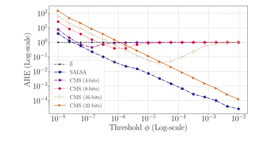
Figure 19: Running CMS with small number of bits and the “$\overline{0}$” algorithm for estimating heavy hitter sizes (2MB) using average relative error metric. The leftmost point corresponds to the standard ARE metric (used in figures 8g and 8h), which considers all flows.

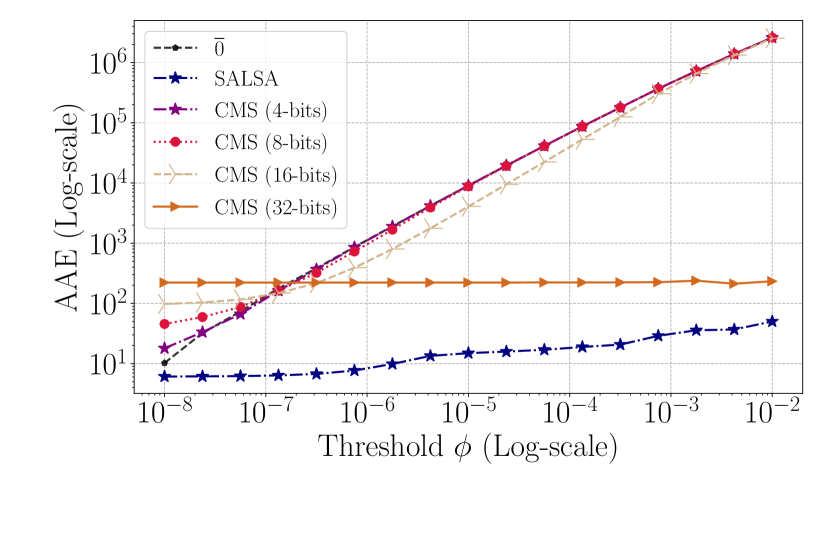
Figure 20: Running CMS with small number of bits and the “$\overline{0}$” algorithm for estimating heavy hitter sizes (2MB) using average absolute error metric. The leftmost point corresponds to the standard AAE metric (used in figures 8e and 8f), which considers all flows.

References

- [1] “Salsa open-source code,” 2020, https://github.com/SALSA-ICDE2021.
- [2] A. Goyal, H. Daumé III, and G. Cormode, “Sketch algorithms for estimating point queries in nlp,” in EMNLP-CoNLL, 2012.
- [3] G. Dittmann and A. Herkersdorf, “Network processor load balancing for high-speed links,” in SPECTS, 2002.
- [4] A. K. Kaushik, E. S. Pilli, and R. C. Joshi, “”Network Forensic Analysis by Correlation of Attacks with Network Attributes”,” in Information and Communication Technologies, 2010.
- [5] R. Ben-Basat, G. Einziger, I. Keslassy, A. Orda, S. Vargaftik, and E. Waisbard, “Memento: making sliding windows efficient for heavy hitters,” in ACM CoNEXT, 2018.
- [6] A. Lall, V. Sekar, M. Ogihara, J. J. Xu, and H. Zhang, “Data streaming algorithms for estimating entropy of network traffic,” in ACM SIGMETRICS/Performance, 2006.
- [7] R. Ben-Basat, X. Chen, G. Einziger, R. Friedman, and Y. Kassner, “Randomized admission policy for efficient top-k, frequency, and volume estimation,” IEEE/ACM Transactions on Networking, 2019.
- [8] P. Roy, A. Khan, and G. Alonso, “Augmented sketch: Faster and more accurate stream processing,” in ACM SIGMOD, 2016.
- [9] T. Yang, J. Jiang, Y. Zhou, L. He, J. Li, B. Cui, S. Uhlig, and X. Li, “Fast and accurate stream processing by filtering the cold,” VLDB J., 2019.
- [10] G. Cormode and S. Muthukrishnan, “An improved data stream summary: The count-min sketch and its applications,” J. Algorithms, 2004.
- [11] N. Hua, B. Lin, J. J. Xu, and H. C. Zhao, “Brick: A novel exact active statistics counter architecture,” in ACM/IEEE ANCS, 2008.
- [12] T. Yang, Y. Zhou, H. Jin, S. Chen, and X. Li, “Pyramid sketch: A sketch framework for frequency estimation of data streams,” 2017, code Available: https://github.com/zhouyangpkuer/Pyramid_Sketch_Framework.
- [13] C. Estan and G. Varghese, “New directions in traffic measurement and accounting,” ACM SIGCOMM, 2002.
- [14] M. Charikar, K. Chen, and M. Farach-Colton, “Finding frequent items in data streams,” in EATCS ICALP, 2002.
- [15] Z. Liu, A. Manousis, G. Vorsanger, V. Sekar, and V. Braverman, “One sketch to rule them all: Rethinking network flow monitoring with univmon,” in ACM SIGCOMM, 2016.
- [16] R. B. Basat, G. Einziger, M. Mitzenmacher, and S. Vargaftik, “Faster and more accurate measurement through additive-error counters,” in IEEE INFOCOM, 2020, code: https://github.com/additivecounters/AEE.
- [17] J. Gong, T. Yang, Y. Zhou, D. Yang, S. Chen, B. Cui, and X. Li, “Abc: a practicable sketch framework for non-uniform multisets,” in 2017 IEEE Big Data, 2017.
- [18] Z. Liu, R. Ben-Basat, G. Einziger, Y. Kassner, V. Braverman, R. Friedman, and V. Sekar, “Nitrosketch: Robust and general sketch-based monitoring in software switches,” in ACM SIGCOMM, 2019.
- [19] Ran Ben Basat, Xiaoqi Chen, Gil Einzinger, Ori Rottenstreich, “Efficient Measurement on Programmable Switches Using Probabilistic Recirculation,” in IEEE ICNP, 2018.
- [20] L. Yang, W. Hao, P. Tian, D. Huichen, L. Jianyuan, and L. Bin, “Case: Cache-assisted stretchable estimator for high speed per-flow measurement,” in IEEE INFOCOM, 2016.
- [21] T. Li, S. Chen, and Y. Ling, “Per-flow traffic measurement through randomized counter sharing,” IEEE/ACM Trans. on Networking, 2012.
- [22] Y. Lu, A. Montanari, B. Prabhakar, S. Dharmapurikar, and A. Kabbani, “Counter braids: a novel counter architecture for per-flow measurement,” in ACM SIGMETRICS, 2008.
- [23] M. Chen and S. Chen, “Counter tree: A scalable counter architecture for per-flow traffic measurement,” in IEEE ICNP, 2015.
- [24] E. Tsidon, I. Hanniel, and I. Keslassy, “Estimators also need shared values to grow together,” in IEEE INFOCOM, 2012.
- [25] C. Hu and B. Liu, “Self-tuning the parameter of adaptive non-linear sampling method for flow statistics,” in CSE, 2009.
- [26] R. Morris, “Counting large numbers of events in small registers,” Commun. ACM, 1978.
- [27] G. Einziger and R. Friedman, “A formal analysis of conservative update based approximate counting,” in ICNC, 2015.
- [28] V. Braverman and R. Ostrovsky, “Zero-one frequency laws,” in ACM STOC, 2010.
- [29] P. Garcia-Teodoro, J. E. Díaz-Verdejo, G. Maciá-Fernández, and E. Vázquez, “Anomaly-based network intrusion detection: Techniques, systems and challenges,” Computers and Security, 2009.
- [30] T. Yang, J. Jiang, P. Liu, Q. Huang, J. Gong, Y. Zhou, R. Miao, X. Li, and S. Uhlig, “Elastic sketch: Adaptive and fast network-wide measurements,” in Proc. of ACM SIGCOMM, 2018.
- [31] K.-Y. Whang, B. T. Vander-Zanden, and H. M. Taylor, “A linear-time probabilistic counting algorithm for database applications,” ACM Transactions on Database Systems (TODS), 1990.
- [32] R. B. Basat, G. Einziger, and R. Friedman, “Fast flow volume estimation,” Pervasive and Mobile Computing, 2018, code available at: https://github.com/ranbenbasat/FAST.
- [33] G. Cormode, “Implementation of heavy hitter algorithms.” [Online]. Available: http://hadjieleftheriou.com/frequent-items/
- [34] J. Teuhola, “Interpolative coding of integer sequences supporting log-time random access,” Information processing & management, 2011.
- [35] A. Elmasry, J. Katajainen, and J. Teuhola, “Improved address-calculation coding of integer arrays,” in SPIRE, 2012.
- [36] S. Cohen and Y. Matias, “Spectral bloom filters,” in ACM SIGMOD, 2003.
- [37] G. S. Manku and R. Motwani, “Approximate frequency counts over data streams,” in VLDB, 2002.
- [38] B. Manes, “Caffeine: A high performance caching library for java 8,” https://github.com/ben-manes/caffeine.
- [39] N. Ivkin, R. B. Basat, Z. Liu, G. Einziger, R. Friedman, and V. Braverman, “I know what you did last summer: Network monitoring using interval queries,” in ACM SIGMETRICS, 2020.
- [40] “The caida equinix-newyork packet trace, 20181220-130000.” 2018.
- [41] “The caida equinix-chicago packet trace, 20160406-130000.” 2016.
- [42] T. Benson, A. Akella, and D. A. Maltz, “Network traffic characteristics of data centers in the wild,” in ACM IMC, 2010.
- [43] “Trending youtube video statistics, kaggle,” 2018, https://www.kaggle.com/datasnaek/youtube-new.
- [44] R. Ben-Basat, G. Einziger, R. Friedman, and Y. Kassner, “Heavy hitters in streams and sliding windows,” in IEEE INFOCOM, 2016.
- [45] B. Krishnamurthy, S. Sen, Y. Zhang, and Y. Chen, “Sketch-based change detection: methods, evaluation, and applications,” in ACM IMC, 2003.
- [46] Student, “The probable error of a mean,” Biometrika, 1908.
- [47] J. Qi, W. Li, T. Yang, D. Li, and H. Li, “Cuckoo counter: A novel framework for accurate per-flow frequency estimation in network measurement,” in ACM/IEEE ANCS, 2019.
- [48] G. Cormode and M. Hadjieleftheriou, “Methods for finding frequent items in data streams,” J. VLDB, 2010.
- [49] D. E. Eisenbud, C. Yi, C. Contavalli, C. Smith, R. Kononov, E. Mann-Hielscher, A. Cilingiroglu, B. Cheyney, W. Shang, and J. D. Hosein, “Maglev: A fast and reliable software network load balancer,” in USENIX NSDI, 2016.
- [50] G. Cormode and H. Jowhari, “L samplers and their applications: A survey,” ACM Comput. Surv., 2019.
- [51] M. Tirmazi, R. Ben Basat, J. Gao, and M. Yu, “Cheetah: Accelerating database queries with switch pruning,” in ACM SIGMOD, 2020.
- [52] “Apache Spark 3 support for Count Min Sketch.” 2020, https://spark.apache.org/docs/3.0.0-preview/api/scala/org/apache/spark/util/sketch/CountMinSketch.html.