Spherical accretion: Bondi, Michel, and rotating black holes

Abstract

In this work we revisit the steady state, spherically symmetric gas accretion problem from the non-relativistic regime to the ultra-relativistic one. We first perform a detailed comparison between the Bondi and Michel models, and show how the mass accretion rate in the Michel solution approaches a constant value as the fluid temperature increases, whereas the corresponding Bondi value continually decreases, the difference between these two predicted values becoming arbitrarily large at ultra-relativistic temperatures. Additionally, we extend the Michel solution to the case of a fluid with an equation of state corresponding to a monoatomic, relativistic gas. Finally, using general relativistic hydrodynamic simulations, we study spherical accretion onto a rotating black hole, exploring the influence of the black hole spin on the mass accretion rate, the flow morphology and characteristics, and the sonic surface. The effect of the black hole spin becomes more significant as the gas temperature increases and as the adiabatic index $\gamma$ stiffens. For an ideal gas in the ultra-relativistic limit ($\gamma=4/3$), we find a reduction of 10 per cent in the mass accretion rate for a maximally rotating black hole as compared to a non-rotating one, while this reduction is of up to 50 per cent for a stiff fluid ($\gamma=2$).

1 Introduction

Gas accretion onto a compact gravitating object is one of the most studied problems in astrophysics. In one of the pioneering works of accretion theory, Bondi (1952) found an analytic solution for the spherically symmetric, steady-state accretion flow of an infinite gas cloud onto a Newtonian point-mass potential. This model has been widely extended and applied in many different fields in astrophysics, from the study of star formation to cosmology. See Armitage (2020) for a recent historical review of this subject.

One of the first studies of spherical accretion onto black holes was the extension of the Bondi solution into the general relativistic regime performed by Michel (1972). In this study, Michel found an analytic solution describing the spherical accretion of a polytropic gas onto a Schwarzschild black hole. A formal mathematical analysis of the Michel solution for a generic equation of state (EoS) can be found in Chaverra et al. (2016). Following Michel’s procedure, other authors have found semi-analytic generalizations for different types of spherically-symmetric (non-rotating) black hole solutions (e.g. Chaverra & Sarbach, 2015; Miller & Baumgarte, 2017; Yang et al., 2021; Abbas & Ditta, 2021). In a recent work, Richards et al. (2021a) explore the non-relativistic and ultra-relativistic limits of Michel’s solution, mainly focusing on a gas with a stiff EoS (values of the adiabatic index larger than 5/3).

In past decades, the spherical accretion Bondi model has been revisited and extended, by including different additional physical ingredients. For example, some authors have taken into account the fluid’s self gravity by solving the coupled Einstein-Euler system in spherical symmetry, either with an analytical treatment (Malec, 1999) or by performing numerical simulations (Lora-Clavijo et al., 2013). Some works have considered the extension of a Bondi-like solution by introducing a low angular momentum fluid  (Abramowicz & Zurek, 1981; Proga & Begelman, 2003; Mach et al., 2018), finding a transition between a quasi-spherical accretion flow and the formation of a thick torus in the equatorial plane. Similarly, there have been works studying spherical accretion in the presence of magnetic fields, either assuming a central dipole (Toropin et al., 1999), or by including a three-dimensional, large-scale weak magnetic field (e.g. Igumenshchev & Narayan, 2002; Ressler et al., 2021). Together with magnetic fields, some works have included the effects of a radiation field, addressing the problem either with a simplified approach (Begelman, 1978, where the author considered a radiation-dominated fluid) or with a self-consistent, radiative-transfer treatment using numerical simulations (McKinney et al., 2014; Weih et al., 2020). In this regard, there have also been studies that extract the shadow of the spherically accreted, optically thin cloud around a non-rotating black hole (Narayan et al., 2019). Other studies have considered the effects of thermal conduction on magnetized spherical accretion flows (Sharma et al., 2008), vorticity (Krumholz et al., 2005), or studied the spherical accretion of a relativistic collisionless kinetic (i.e. a Vlasov) gas (Rioseco & Sarbach, 2017a).

Recent works have also studied deviations away from spherical symmetry by introducing large-scale, small-amplitude density anisotropies, finding that even a slight equator-to-poles density contrast can drastically modify Bondi’s solution, giving rise to an inflow-outflow configuration consisting of equatorial accretion and a bipolar outflow. The resulting steady-state configuration, dubbed choked accretion, was studied in Aguayo-Ortiz et al. (2019) at the Newtonian level and, within a general relativistic framework, in Tejeda et al. (2020) and Aguayo-Ortiz et al. (2021) for Schwarzschild and Kerr black holes, respectively. In these series of works, it was found that the total mass flux that reaches the central accretor is of the order of magnitude of the corresponding Bondi mass accretion rate, while all the excess flux is redirected by the density gradient as outflow. Under the conditions explored so far, the Bondi mass accretion rate acts as a threshold value delimiting whether a given incoming flow becomes choked and prone to the ejection of a bipolar outflow.

Among the astrophysical applications of the spherical accretion model, we mention the study of gas accretion in an expanding Universe (Colpi et al., 1996), the formation and growth of primordial black holes in the early stages of the Universe (Zel’dovich & Novikov, 1967; Carr, 1981; Karkowski & Malec, 2013; Lora-Clavijo et al., 2013), and the accretion onto a mini black hole from the interior of a neutron star (Kouvaris & Tinyakov, 2014; Génolini et al., 2020; Richards et al., 2021b). On the other hand, the Bondi solution allows to estimate, by providing useful characteristic scale tools, the accretion and growth rate of the central supermassive black hole at the centre of galaxies (Maraschi et al., 1974; Moscibrodzka, 2006; Ciotti & Pellegrini, 2017; Moffat, 2020) and active galactic nuclei (Krolik & London, 1983; Russell et al., 2013, 2015), where observations provide information only from regions far away from the central accretor. Similarly, the Bondi prescription is often used in cosmological simulations as a sub-grid model to estimate the accretion rate of gas onto supermassive black holes at galactic centres (Davé et al., 2019).

On the other hand, the analytic study of accretion flows onto rotating black holes has proven more challenging. Notably, Petrich, Shapiro & Teukolsky (1988) found a full analytic solution that describes the accretion of an irrotational, ultra-relativistic stiff fluid onto a rotating Kerr black hole. However, a main caveat of this solution is that it requires a rather specific, unphysical EoS, in which the sound speed equals the speed of light. Assuming a more general EoS, Beskin & Pidoprygora (1995) studied the problem of spherical accretion onto a slowly rotating black hole by means of a perturbative analysis, and Pariev (1996) extended this work to the case of a rapidly rotating black hole. Both Beskin & Pidoprygora (1995) and Pariev (1996) considered only small deviations away from a Bondi background solution, in other words, these studies where limited to the case of non-relativistic values for the gas temperature at infinity. Even though this assumption might be reasonable in many astrophysical settings, the determination of the effect of the black hole spin on the accretion flow given an arbitrary gas temperature remains an open problem.

The applications of Bondi’s model in most of the aforementioned works consider the gas accretion in the non-relativistic regime, not to mention that they neglect the rotation of the black hole. The reason for this is that the Bondi scale factors are estimated and measured at distances far away from the central black hole, where it is safe to neglect relativistic effects. Nevertheless, in order to analyse the exact differences between the Bondi solution and the relativistic extension performed by Michel, as well as to assess the effect of the black hole spin, it is important to perform a quantitative study of the consequences of having relativistic gas temperatures and strong gravity fields in the vicinity of a rotating black hole.

In this work we study the spherically symmetric gas accretion problem from the non-relativistic regime to the ultra-relativistic one, considering both rotating and non-rotating black holes. We first perform a detailed comparison between the Bondi (1952) and Michel (1972) models by studying the behaviour of the relativistic solution across a wide range of values of the gas temperature. In particular, we discuss in detail the isothermal, the non-relativistic, and the ultra-relativistic limits of the Michel solution. We then extend Michel’s solution to the case of a monoatomic gas obeying a relativistic EoS (Jüttner, 1911; Taub, 1948; Synge, 1957). We also revisit Petrich et al. (1988)’s analytic solution and apply it to the particular case of a spherically symmetric accretion flow onto a Kerr black hole. Finally, by means of two dimensional (2D) general relativistic hydrodynamic simulations, we perform a quantitative study of the effect that the black hole spin has on the spherical accretion problem, focusing in particular on its effects on the mass accretion rate and on the flow morphology for several EoS. As part of this study, we show how, under the appropriate limits, the obtained numerical results coincide with the analytic solutions of Michel (1972) and Petrich et al. (1988).

The paper is organised as follows. In Section 2 we discuss the analytic solutions of Bondi (1952), Michel (1972) and Petrich et al. (1988). In Section 3 we present our numerical study of the spherical accretion of a perfect fluid onto a rotating black hole. Finally, in Section 4 we present a summary of the main results found in this article and give our conclusions. Technical details regarding the isothermal and non-relativistic limits of the Michel solution, the correct determination of the sonic surface for flows on rotating black holes, and orthonormal frames are discussed in appendices.

2 Analytic solutions

In this section we review three analytic solutions describing a steady-state, spherical accretion flow onto a central massive object. We start by revisiting the Bondi (1952) solution and perform a detailed comparison with the relativistic extension found by Michel (1972). Then, we extend the latter solution by considering the more realistic equation of state for a monoatomic relativistic gas introduced by Jüttner (1911). Finally, in order to give a description of accretion onto a rotating black hole, we also discuss the ultra-relativistic, stiff solution found by Petrich et al. (1988) in the case of spherical symmetry.

2.1 Bondi solution

In the Bondi (1952) analytic solution, one considers an infinite, spherically symmetric gas cloud accreting onto a Newtonian central object of mass $M$. At large distances, the gas cloud is assumed to be at rest and characterised by a homogeneous density $\rho_{\text{\tiny$\infty$ }}$ and pressure $P_{\text{\tiny$\infty$ }}$. Note that, using an ideal gas EoS, we can alternatively describe the state of the fluid in terms of the dimensionless gas temperature $\Theta$ defined as:

$$\Theta=\frac{k_{\rm B}\,T}{\bar{m}\,c^{2}}=\frac{P}{\rho\,c^{2}},$$ (2.1)

where $c$ is the speed of light, $k_{\rm B}$ Boltzmann’s constant, and $\bar{m}$ the average rest mass of the gas particles. As reference values, $\Theta\simeq T/(10^{13}\,{\rm K})$ for atomic hydrogen gas and $\Theta\simeq T/(10^{10}\,{\rm K})$ for an electron-positron plasma.

Under the assumptions of steady-state and spherical symmetry, the equations governing the Bondi accretion flow are the continuity equation and the radial Euler equation, i.e.

$$\frac{1}{r^{2}}\frac{\mathrm{d}}{\mathrm{d}r}\left(r^{2}\rho\,v\right)=0,$$ (2.2a)

$$v\frac{\mathrm{d}v}{\mathrm{d}r}+\frac{1}{\rho}\frac{\mathrm{d}P}{\mathrm{d}r}+\frac{GM}{r^{2}}=0,$$ (2.2b)

where $v=|\mathrm{d}r/\mathrm{d}t|$ is the radial velocity of the fluid.

Considering that, in addition to the ideal gas EoS, the fluid obeys a polytropic relation $P=K\rho^{\gamma}$, with $K=\mathrm{const.}$ and $\gamma$ the adiabatic index (assumed to lie in the range $1\leq\gamma\leq 2$), equations (2.2a) and (2.2b) can be integrated:

$$4\pi\,r^{2}\rho\,v=\dot{M} =\mathrm{const.},$$ (2.3a)

$$\frac{v^{2}}{2}+\mathscr{h}-\frac{GM}{r}=\mathscr{h}{\text{\tiny$\infty$ }} =\mathrm{const.},$$ (2.3b)

where

$$\mathscr{h}=\left(\frac{\gamma}{\gamma-1}\right)\frac{P}{\rho}=\frac{\gamma\,\Theta\,c^{2}}{\gamma-1}=\frac{\mathcal{C}^{2}}{\gamma-1}$$ (2.4)

is the specific enthalpy and $\mathcal{C}:=\sqrt{\partial P/\partial\rho}$ the adiabatic speed of sound. Note that equation (2.4) is only valid for $\gamma>1$. In the isothermal case, where $\gamma=1$ and $\Theta\equiv\Theta{\text{\tiny$\infty$ }}=\mathcal{C}^{2}_{\text{\tiny$\infty$ }}/c^{2}$, equation (2.4) needs to be replaced by

$$\mathscr{h}-\mathscr{h}_{\text{\tiny$\infty$ }}=\mathcal{C}^{2}_{\text{\tiny$\infty$ }}\ln\left(\frac{\rho}{\rho{\text{\tiny$\infty$ }}}\right).$$ (2.5)

In addition to the steady-state and spherical symmetry conditions, Bondi also assumed that the flow is transonic, i.e. that there exists a radius $r_{s}$ at which the fluid’s radial velocity equals the local speed of sound. From equations (2.2a) and (2.2b), it is simple to calculate that the fluid at the sonic radius, $r_{s}$, satisfies

$$r_{s}=\frac{GM}{2v_{s}^{2}},$$ (2.6a)

$$v_{s}=\mathcal{C}_{s}=\mathcal{C}_{\text{\tiny$\infty$ }}\left(\frac{2}{5-3\gamma}\right)^{1/2}.$$ (2.6b)

The transonic solution found by Bondi is unique and maximises the accretion rate onto the central object, which, in turn, is given by

$$\dot{M}_{\rm B}=4\pi\,\lambda_{\rm B}(GM)^{2}\frac{\rho_{\text{\tiny$\infty$ }}}{\mathcal{C}^{3}_{\text{\tiny$\infty$ }}},$$ (2.7)

where $\lambda_{\rm B}$ is a numerical factor of order one that depends only on $\gamma$ and is given by

$$\lambda_{\rm B}=\frac{1}{4}\left(\frac{2}{5-3\gamma}\right)^{\frac{5-3\gamma}{2(\gamma-1)}}.$$ (2.8)

The accretion rate given in equation (2.7) is only valid for $\gamma\leq 5/3$. In order to discuss the $\gamma>5/3$ case, one must necessarily account for general relativistic effects as we shall see in Section 2.2. Particular values for $\lambda_{\rm B}$ in equation (2.8) are

$$\lambda_{\rm B}(5/3)=1/4,$$

$$\lambda_{\rm B}(4/3)=1/\sqrt{2}\simeq 0.71,$$

$$\lambda_{\rm B}(1)=\mathrm{e}^{3/2}/4\simeq 1.12.$$

An interesting characteristic of the Bondi solution is that it can be written in a scale-free form with respect to the mass of the central object $M$ and the thermodynamic state of the fluid ($\rho_{\text{\tiny$\infty$ }}$, $P_{\text{\tiny$\infty$ }}$) by adopting $r_{\mathrm{B}}=GM/C^{2}_{\text{\tiny$\infty$ }}$, $\mathcal{C}_{\text{\tiny$\infty$ }}$, and $\rho_{\text{\tiny$\infty$ }}$ as units of length, velocity, and density, respectively. In other words, a global solution of the Bondi accretion problem is fully characterised once a given value for the adiabatic index $\gamma$ is provided. Once the value for the mass accretion rate of Bondi’s solution for a given $\gamma$ is known, one can go back to equations (2.3a)–(2.4) and solve numerically the corresponding algebraic system of non-linear equations to obtain $\rho$, $P$, and $v$ as a function of radius. See Figure 1, for an example where we show the resulting Mach number ($\mathcal{M}=v/\mathcal{C}$) as a function of radius, for the solution with $\gamma=4/3$ (red line).

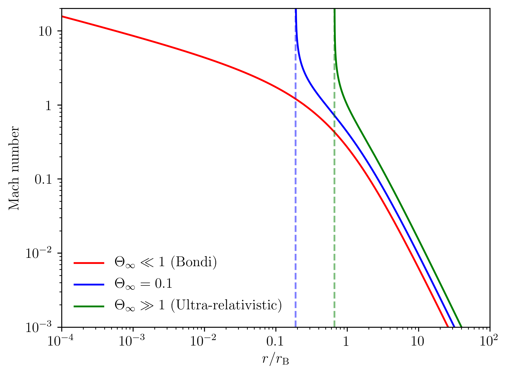
Figure 1: Mach number as a function of radius for the case of a $\gamma=4/3$ polytrope and for three asymptotic temperatures. Note that the non-relativistic limit ($\Theta_{\text{\tiny$\infty$ }}\ll 1$) corresponds to the Bondi solution. The vertical dashed lines show the location of the black hole’s event horizon for $\Theta_{\text{\tiny$\infty$ }}=0.1$ and $\Theta_{\text{\tiny$\infty$ }}\gg 1$. In all cases the accretion flow has transitioned from subsonic to supersonic before crossing the event horizon. The horizontal axis is scaled in units of the Bondi radius $r_{\mathrm{B}}=GM/C^{2}_{\text{\tiny$\infty$ }}$.

2.2 Michel solution

As mentioned in the introduction, a general relativistic extension of the Bondi solution was presented by Michel (1972) who considered a Schwarzschild black hole as central accretor. In what follows we review Michel’s solution and discuss its main differences with respect to the Bondi model. It is important to remark that the Michel solution assumes an ideal gas EoS that follows a polytropic relation $P=K\,\rho^{\gamma}$, where, as in the previous section, $\rho$ is the rest-mass density. Note however that this assumption is limited in general. For example, for a monoatomic ideal gas, it is only valid at non-relativistic temperatures (for which $\gamma=5/3$), or at ultra-relativistic temperatures (for which $\gamma=4/3$). In order to study the whole temperature domain in a consistent way, the polytropic restriction must be dropped and a relativistic EoS (as derived, for example, from relativistic kinetic theory, Synge, 1957) must be adopted. We discuss the extension of the Michel solution to such a relativistic EoS in Section 2.3.

As in the Newtonian case, the governing equations are the conservation of mass and energy, i.e. the continuity equation and the requirement for the energy-momentum tensor to be divergence-free,

$$\left(\rho\,U^{\mu}\right)_{;\mu}=0,$$ (2.9a)

$$\left(T^{\mu\nu}\right)_{;\mu}=0,$$ (2.9b)

where the semicolon stands for covariant derivative, $U^{\mu}$ is the fluid four-velocity, $T^{\mu\nu}=\rho\,h\,U^{\mu}U^{\nu}+p\,g^{\mu\nu}$ is the stress-energy tensor of a perfect fluid, $h=1+\mathscr{h}$ is the specific relativistic enthalpy, and $g^{\mu\nu}$ denote the components of the inverse of the Schwarzschild metric

$$ds^{2}=-\left(1-\frac{2M}{r}\right)\mathrm{d}t^{2}+\frac{\mathrm{d}r^{2}}{1-\frac{2M}{r}}+r^{2}\left(\mathrm{d}\theta^{2}+\sin^{2}\theta\mathrm{d}\phi^{2}\right).$$ (2.10)

In order to ease the notation, we adopt geometrised units in which $G=c=1$.

It is useful to recall at this point that, in the relativistic regime, the fluid’s sound speed is defined as

$$\mathcal{C}^{2}:=\frac{\rho}{h}\frac{\partial h}{\partial\rho}=\frac{\gamma}{h}\frac{P}{\rho}=\frac{\gamma}{h}\,\Theta,$$ (2.11)

where, for the second equal sign, we have substituted the polytropic relation for a perfect fluid. Also note that equation (2.11) can be recast to express $h$ in terms of $\mathcal{C}$ or $\Theta$ as

$$h=\frac{1}{1-\mathcal{C}^{2}/(\gamma-1)}=1+\frac{\gamma}{\gamma-1}\Theta.$$ (2.12)

Under the conditions of steady-state and spherical symmetry, equations (2.9a) and (2.9b) reduce to

$$\frac{\mathrm{d}}{\mathrm{d}r}\left(r^{2}\rho\,U^{r}\right)=0,$$ (2.13a)

$$\frac{\mathrm{d}}{\mathrm{d}r}\left(r^{2}\rho\,h\,U_{t}\,U^{r}\right)=0,$$ (2.13b)

which, upon integration, can be rewritten as

$$4\pi\,r^{2}\rho\,u=\dot{M}=\mathrm{const.},$$ (2.14a)

$$h\left(1-\frac{2M}{r}+u^{2}\right)^{1/2}=h{\text{\tiny$\infty$ }}=\mathrm{const.},$$ (2.14b)

where $u=|U^{r}|$.

As in the Newtonian case, there exists a unique, transonic solution where the fluid is at rest asymptotically far away from the central object and that is regular across the black hole’s event horizon (Chaverra & Sarbach, 2015; Chaverra et al., 2016). In order to find the defining conditions that are satisfied at the sonic point $r_{s}$, it is useful to combine equations (2.13a) and (2.13b) into the following differential equation

$$\begin{split}\bigg{[}1-\frac{\mathcal{C}^{2}}{u^{2}}\bigg{(}1&-\frac{2M}{r}+u^{2}\bigg{)}\bigg{]}u\frac{\mathrm{d}u}{\mathrm{d}r}=\\ &-\frac{M}{r^{2}}+2\frac{\mathcal{C}^{2}}{r}\left(1-\frac{2M}{r}+u^{2}\right).\end{split}$$ (2.15)

By requiring that both sides of this equation vanish simultaneously at $r_{s}$, the following conditions arise

$$r_{s}=\frac{1}{2}\frac{M}{u_{s}^{2}},$$ (2.16a)

$$u_{s}^{2}=\frac{\mathcal{C}_{s}^{2}}{1+3\,\mathcal{C}_{s}^{2}}.$$ (2.16b)

If we introduce $V$ as the norm of the fluid’s three-velocity as measured by local static observers, given in this case by

$$V=\left(1-\frac{2M}{r}\right)^{-1}\left|\frac{U^{r}}{U^{t}}\right|,$$ (2.17)

from equations (2.16a) and (2.16b) it follows that $V_{s}=\mathcal{C}_{s}$, which justifies calling $r_{s}$ the sonic radius.

On the other hand, a relationship between the fluid state at infinity and at the sonic point can be obtained by substituting equations (2.16a) and (2.16b) into equation (2.14b). Doing this results in the following cubic equation for $h_{s}$ (see Tejeda et al., 2020, Appendix A)

$$h_{s}^{3}-(3\gamma-2)h^{2}_{\text{\tiny$\infty$ }}h_{s}+3(\gamma-1)h^{2}_{\text{\tiny$\infty$ }}=0,$$ (2.18)

as well as the corresponding equation for the sound speed

$$\mathcal{C}_{s}^{2}=\frac{1}{3}\left(\frac{h_{s}^{2}}{h^{2}_{\text{\tiny$\infty$ }}}-1\right).$$ (2.19)

The polynomial in equation (2.18) has three real roots but only one satisfies $h_{s}>1$ and thus has physical meaning. This root is given by

$$h_{s}=2\,h{\text{\tiny$\infty$ }}\,\sqrt{\gamma-\frac{2}{3}}\,\sin\left(\Psi+\frac{\pi}{6}\right),$$ (2.20)

where

$$\Psi=\frac{1}{3}\arccos\left[\frac{3(\gamma-1)}{2\,h_{\text{\tiny$\infty$ }}}\left(\gamma-\frac{2}{3}\right)^{-3/2}\right].$$ (2.21)

Substituting these results back into equation (2.14a), the mass accretion rate can be expressed in terms of the asymptotic state of the fluid as

$$\dot{M}_{\rm M}=4\pi\,\lambda_{\rm M}M^{2}\frac{\rho_{\text{\tiny$\infty$ }}}{\mathcal{C}^{3}_{\text{\tiny$\infty$ }}},$$ (2.22)

where now the numerical factor $\lambda_{\rm M}$ depends not only on $\gamma$ but also on the asymptotic state of the fluid and is given by

$$\lambda_{\rm M}=\frac{1}{4}\left(\frac{h_{s}}{h_{\text{\tiny$\infty$ }}}\right)^{\frac{3\gamma-2}{\gamma-1}}\left(\frac{\mathcal{C}_{s}}{\mathcal{C}_{\text{\tiny$\infty$ }}}\right)^{\frac{5-3\gamma}{\gamma-1}}.$$ (2.23)

In Figure 2 we show the dependence of $\lambda_{\mathrm{M}}$ on $\Theta_{\text{\tiny$\infty$ }}$ for several different values of the adiabatic index $\gamma$. From this figure, it is clear that for $\gamma\leq 5/3$ in the non-relativistic limit $(\Theta_{\text{\tiny$\infty$ }}\ll 1)\ \lambda_{\mathrm{M}}\to\lambda_{\mathrm{B}}$, as expected. We stress that the mass accretion rate given in equation (2.22) is only a measure for the flux of rest-mass (particle number times the average rest-mass per particle) onto the central black hole. If interested in computing the actual growth rate of the black hole’s mass, the total energy advected by each fluid particle should be taken into account by computing the energy accretion rate (for further details see Aguayo-Ortiz et al., 2021). Since for the present problem the fluid is assumed to be at rest at infinity, one only needs to multiply $\dot{M}_{\rm M}$ in equation (2.22) by $h_{\text{\tiny$\infty$ }}$ to obtain this rate, i.e.

$$\dot{\mathcal{E}}_{\rm M}=4\pi\,\lambda_{\rm M}M^{2}\rho_{\text{\tiny$\infty$ }}\left(\frac{1}{\gamma\Theta_{\text{\tiny$\infty$ }}}+\frac{1}{\gamma-1}\right)^{5/2}\gamma\Theta_{\text{\tiny$\infty$ }}.$$ (2.24)

In contrast to the Bondi solution, where the asymptotic speed of sound $\mathcal{C}_{\text{\tiny$\infty$ }}$ is the only characteristic velocity, the Michel solution naturally features the speed of light as an additional characteristic velocity. Consequently, the Michel solution can only be rendered scale invariant with respect to $M$ and $\rho_{\infty}$. Therefore, in addition to the adiabatic index $\gamma$, to completely describe a given solution one must also specify $\mathcal{C}_{\text{\tiny$\infty$ }}$ or, alternatively, $\Theta_{\text{\tiny$\infty$ }}$. In what follows we shall use $\Theta_{\text{\tiny$\infty$ }}$ as the dynamically relevant parameter describing the state of the fluid asymptotically far away from the central object.

Examples of the resulting Mach number $\mathcal{M}$ for a $\gamma=4/3$ polytrope and various asymptotic temperatures: $\Theta_{\text{\tiny$\infty$ }}=10^{-4},\,0.1,\,10^{4}$ are also shown in Figure 1. Note that, in the relativistic case we have defined

$$\mathcal{M}=\frac{V\sqrt{1-\mathcal{C}^{2}}}{\mathcal{C}\sqrt{1-V^{2}}}.$$ (2.25)

As we can see from this figure, in all cases the accretion flow transitions from being subsonic to supersonic before reaching the event horizon (indicated by the dashed lines). Also, the non-relativistic limit ($\Theta_{\text{\tiny$\infty$ }}\ll 1$) coincides with the Bondi solution.

In Figures 3 and 4 we show, respectively, the sonic radius $r_{s}$ and the mass accretion rate $\dot{M}_{\mathrm{M}}$ as functions of $\Theta_{\text{\tiny$\infty$ }}$ and for several representative values of $\gamma$. By examining these figures, and analysing in detail the result obtained in equation (2.22), three interesting limits can be identified (isothermal, non-relativistic and ultra-relativistic). In what follows, we list the main conclusions that can be drawn in each case, leaving detailed calculations to Appendix A.

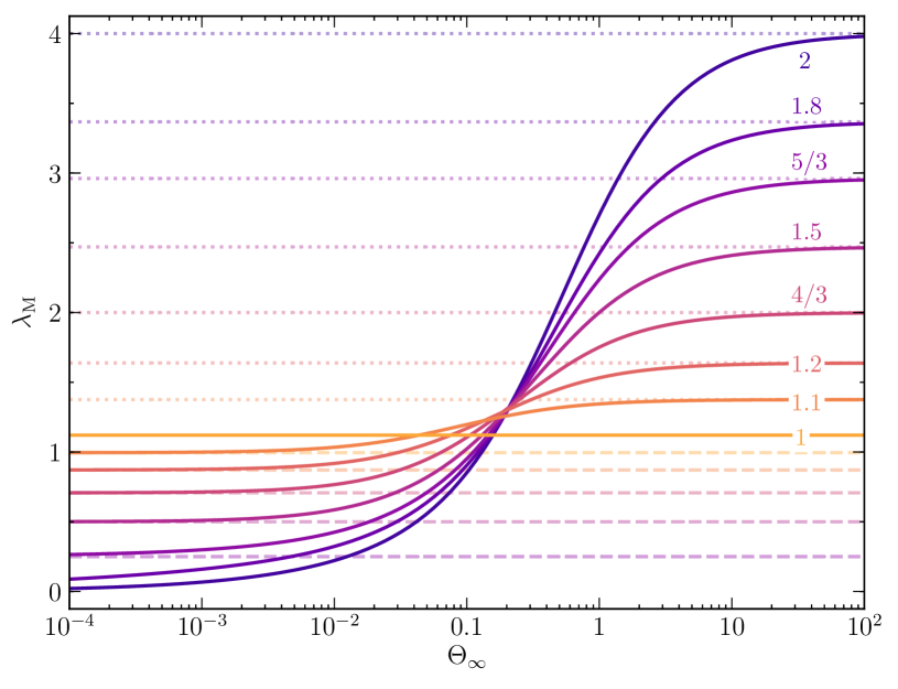
Figure 2: Numerical factor $\lambda_{\rm M}$ in the definition of the mass accretion rate of the Michel solution (equation 2.23) as a function of the dimensionless temperature $\Theta{\text{\tiny$\infty$ }}$ and for different values of $\gamma$ as indicated by the labels on top of each curve. In the non-relativistic limit $\Theta_{\text{\tiny$\infty$ }}\ll 1$ and for values of $\gamma\leq 5/3$, the curves asymptotically approach the values corresponding to $\lambda_{\rm B}$ (dashed horizontal lines) of the Bondi solution in equation (2.7). In the ultra-relativistic limit $\Theta_{\text{\tiny$\infty$ }}\gg 1$, the curves asymptotically approach the value given in equation (2.28).

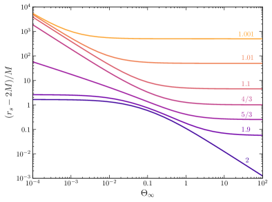
Figure 3: Distance between the sonic radius $r_{s}$ and the black hole’s event horizon radius $r_{+}=2M$ in the Michel solution as a function of the dimensionless temperature $\Theta{\text{\tiny$\infty$ }}$ and for different values of $\gamma$ as indicated by the labels on top of each curve.

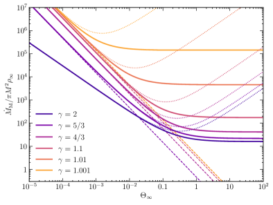
Figure 4: Mass accretion rate of the Michel solution $\dot{M}_{\mathrm{M}}$ as a function of $\Theta_{\text{\tiny$\infty$ }}$ and for several representative values of $\gamma$. The dashed lines represent the corresponding Bondi mass accretion rate $\dot{M}_{\mathrm{B}}$ in cases with $\gamma\leq 5/3$. The dotted lines show the corresponding energy accretion rate (see equation 2.24). Note that once $\Theta_{\text{\tiny$\infty$ }}\gtrsim 10^{-2}$, the differences between Bondi’s and Michel’s solutions become of order one and that this difference actually diverges as $\Theta_{\text{\tiny$\infty$ }}\to\infty$.

(i) Isothermal limit

The isothermal limit corresponds to the condition when $\gamma\to 1$. From Figure 3 we note that, within this limit and for all temperatures $\Theta_{\infty}$, the sonic radius recedes without limit from the event horizon. As we prove in Appendix A, the Michel solution (with a suitable rescaling) converges to the Newtonian Bondi solution with an EoS as given by equation (2.5). Thus, the isothermal case can be entirely described within the context of Newtonian physics, even for large temperatures that would ordinarily be associated with an ultra-relativistic regime.

(ii) Non-relativistic limit

This limit is described by the condition $\Theta_{\infty}\ll 1$ which implies $h_{\infty}\rightarrow 1$. As expected, and as is already apparent from Figures 1 and 2, in this limit the Michel solution converges to the Bondi one and expressions like the mass accretion rate (equation 2.22) reduce to their non-relativistic counterparts (equation 2.7). Nevertheless, this is only true for $\gamma\leq 5/3$. When $\gamma>5/3$ a qualitative change takes place in Michel’s solution. From Figure 3 it is clear that for $\gamma<5/3$ the value of $r_{s}$ grows to infinity as $\Theta_{\infty}^{-1}$ (as in the Bondi solution), while it converges to a finite distance from the event horizon for $\gamma>5/3$. This is indicative that the cases with $\gamma>5/3$ cannot be described with Newtonian physics, even in the low temperature limit. As shown in Appendix A, when $\Theta_{\text{\tiny$\infty$ }}\ll 1$ and $\gamma>5/3$, one finds that $r_{s}$ converges to a finite value and $h_{s}>1$, while the resulting mass accretion rate converges to

$$\dot{M}_{\rm M}\to\pi h_{s}^{\frac{3\gamma-2}{\gamma-1}}\mathcal{C}_{s}^{\frac{5-3\gamma}{\gamma-1}}M^{2}\rho_{\text{\tiny$\infty$ }}\,\mathcal{C}^{-\frac{2}{\gamma-1}}_{\text{\tiny$\infty$ }}.$$ (2.26)

(iii) Ultra-relativistic limit

Finally, we discuss the case where $\Theta_{\text{\tiny$\infty$ }}\gg 1$. From Figure 3 it is clear that $r_{s}$ converges to a finite value strictly larger than the event horizon radius for all values of $\gamma$, with the exception of a stiff EoS $\gamma=2$, in which case $r_{s}\to r_{+}$ as $\Theta_{\text{\tiny$\infty$ }}\to\infty$. Moreover, within this limit equation (2.20) reduces to

$$\frac{h_{s}}{h_{\text{\tiny$\infty$ }}}\to\sqrt{3\gamma-2},$$ (2.27)

from which one also obtains $\mathcal{C}_{s}/\mathcal{C}_{\text{\tiny$\infty$ }}\to 1$ and, hence,

$$\lambda_{\rm M}\to\frac{1}{4}(3\gamma-2)^{\frac{3\gamma-2}{2(\gamma-1)}}.$$ (2.28)

This limit value grows monotonically from $\mathrm{e}^{3/2}\simeq 1.12$ to $4$ as $\gamma$ increases from $1$ to $2$ (see Figure 2). From this result, and as is also clear from Figure 4, one sees that the mass accretion rate becomes independent of $\Theta_{\text{\tiny$\infty$ }}$, rapidly approaching the constant value

$$\dot{M}_{\mathrm{M}}\to\pi M^{2}\rho_{\text{\tiny$\infty$ }}(3\gamma-2)^{\frac{3\gamma-2}{2(\gamma-1)}}(\gamma-1)^{-3/2}.$$ (2.29)

In comparison, the Bondi mass accretion rate steadily decreases as $\Theta^{-3/2}_{\text{\tiny$\infty$ }}$ as the temperature increases. Therefore, the difference between $\dot{M}_{\mathrm{B}}$ and $\dot{M}_{\mathrm{M}}$ becomes arbitrarily large when $\Theta_{\text{\tiny$\infty$ }}\gg 1$. Also note that the energy accretion rate is not monotonic; it decreases for small temperatures but increases for large ones, eventually growing linearly in $\Theta_{\text{\tiny$\infty$ }}$ (see equation 2.24 and Figure 4). A similar qualitative behaviour has been observed for the accretion of a Vlasov gas (Rioseco & Sarbach, 2017b). This is a remarkable difference between the Bondi and Michel solutions that, to the best of our knowledge, had not been discussed in the literature before. We can track the reason behind this behaviour by examining equations (2.7) and (2.22). Even though the factor $\mathcal{C}^{-3}_{\text{\tiny$\infty$ }}$ appears in both expressions, this factor behaves drastically differently when $\Theta_{\text{\tiny$\infty$ }}\gtrsim 1$. For a perfect fluid in Newtonian hydrodynamics, one simply has $\mathcal{C}^{2}=\gamma\,\Theta$ and, thus, as the temperature increases so does the speed of sound without limit. Consequently, and as can be seen in Figure 4, the Bondi mass accretion rate decreases to small values as the asymptotic gas temperature increases. On the other hand, in relativistic hydrodynamics one has

$$\mathcal{C}^{2}=\frac{\gamma(\gamma-1)\Theta}{\gamma-1+\gamma\,\Theta},$$

that, in the limit $\Theta_{\text{\tiny$\infty$ }}\gg 1$, implies that the speed of sound attains a maximum value given by $\mathcal{C}_{\text{\tiny$\infty$ }}\to\sqrt{\gamma-1}$. Therefore, when $\Theta_{\text{\tiny$\infty$ }}\gg 1$, $\dot{M}_{\mathrm{M}}$ becomes independent of $\Theta_{\text{\tiny$\infty$ }}$.

2.3 Michel solution with relativistic EoS

In the previous subsection we revisited spherical accretion of a fluid that follows an ideal gas EoS and that is restricted to obey a polytropic relation. As mentioned before, assuming a monoatomic gas, this restriction is only valid in the non-relativistic limit ($\Theta_{\text{\tiny$\infty$ }}\ll 1$) with $\gamma=5/3$ or in the ultra-relativistic one ($\Theta_{\text{\tiny$\infty$ }}\gg 1$) with $\gamma=4/3$. Nevertheless, as it was shown by Taub (1948), in the relativistic case ($\Theta_{\text{\tiny$\infty$ }}\sim 1$) the polytropic restriction is not physical and has to be dropped.

In this subsection we extend the Michel solution to the case of a gas obeying an appropriate EoS for the relativistic regime. As derived from relativistic kinetic theory, the EoS of an ideal, monoatomic gas can be written as (Jüttner, 1911; Synge, 1957; Falle & Komissarov, 1996)

$$h=\frac{K_{3}(1/\Theta)}{K_{2}(1/\Theta)},$$ (2.30)

where, as before $\Theta=P/\rho$, and $K_{n}$ is the $n$th-order modified Bessel function of the second kind.

By additionally imposing the adiabatic condition (i.e. isentropic flow), one obtains the following relation between $\rho$ and $\Theta$ (see e.g., Appendix B of Chavez Nambo & Sarbach, 2020)

$$\frac{\rho}{\rho_{\text{\tiny$\infty$ }}}=\frac{f(\Theta)}{f(\Theta_{\text{\tiny$\infty$ }})},$$ (2.31a)

$$f(\Theta)=\Theta\,K_{2}(1/\Theta)\,\exp\left[\frac{1}{\Theta}\frac{K_{1}(1/\Theta)}{K_{2}(1/\Theta)}\right].$$ (2.31b)

Meanwhile, the speed of sound in this case is given by

$$\mathcal{C}^{2}=\frac{\bar{\gamma}\,\Theta}{h},$$ (2.32)

where $\bar{\gamma}$ is the effective adiabatic index, defined as

$$\bar{\gamma}:=\frac{\rho}{P}\frac{\partial P}{\partial\rho}=\frac{h}{\Theta}\mathcal{C}^{2}.$$ (2.33)

In contrast to the polytropic gas treatment discussed before, $\bar{\gamma}$ is not a constant but rather a function of the temperature that can be calculated explicitly as

$$\bar{\gamma}=\frac{h^{\prime}}{h^{\prime}+\Theta^{2}},$$ (2.34)

where the prime refers to derivatives with respect to the argument of the modified Bessel functions, i.e. $h^{\prime}=\mathrm{d}[K_{3}(x)/K_{2}(x)]/\mathrm{d}x$. With this definition of $\bar{\gamma}$ it follows that, as expected, for non-relativistic temperatures, $\bar{\gamma}\to 5/3$ while, in the ultra-relativistic limit, $\bar{\gamma}\to 4/3$.

In order to derive the appropriate governing equations in this case, we first notice that equation (2.18) should be replaced with

$$h_{s}^{2}=h^{2}_{\text{\tiny$\infty$ }}(1+3\,\mathcal{C}_{s}^{2})=h^{2}_{\text{\tiny$\infty$ }}\left[1+\frac{3\Theta_{s}}{h_{s}}\left(\frac{h_{s}^{\prime}}{h_{s}^{\prime}+\Theta_{s}^{2}}\right)\right],$$ (2.35)

which, in contrast to equation (2.18), does not allow for an analytic solution. Nevertheless, it can be easily solved numerically using any standard root finding algorithm.

The corresponding mass accretion rate is obtained by evaluating equation (2.14a) at the sonic point, i.e.

$$\dot{M}=4\pi\,r_{s}^{2}\,\rho_{s}\,u_{s},$$ (2.36)

and, by applying the conditions given by equations (2.16a) and (2.16b) that, together with equation (2.31a), result in

$$\dot{M}=\pi M^{2}\rho_{\text{\tiny$\infty$ }}\frac{(1+3\,\mathcal{C}_{s}^{2})}{\mathcal{C}_{s}^{3}}^{3/2}\frac{f(\Theta_{s})}{f(\Theta_{\text{\tiny$\infty$ }})}.$$ (2.37)

In practice, to calculate the resulting mass accretion rate for a given asymptotic state $(\rho_{\text{\tiny$\infty$ }},\Theta_{\text{\tiny$\infty$ }})$, we numerically solve equation (2.35) to obtain $\Theta_{s}$, from which we can compute $h_{s}$ and $\mathcal{C}_{s}$ via equations (2.30) and (2.32), respectively, and then substitute these values into equation (2.37).

In Figure 5 we show the resulting mass accretion rate as a function of $\Theta_{\text{\tiny$\infty$ }}$ for the relativistic EoS and compare it with the corresponding values for $\gamma=5/3,\,4/3$ polytropes. From this figure we can see that the result obtained with the relativistic EoS provides a smooth transition between the polytropic approximations as the temperature transitions from non-relativistic values to the ultra-relativistic regime. We also show the approximation to the relativistic EoS proposed by Ryu et al. (2006), where,

$$h=2\frac{6\Theta^{2}+4\Theta+1}{3\Theta+2},$$ (2.38)

and which provides an accurate estimate to the mass accretion rate to within 2$\%$. This comparison is relevant for this work, given that, for some of the numerical simulations presented in Section 3, we have adopted this proxy for the implementation of the relativistic EoS.

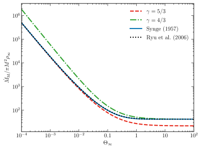
Figure 5: Mass accretion rate in Michel’s model for a gas described by a relativistic EoS (Synge, 1957). The resulting rate converges to a $\gamma=5/3$ polytrope when $\Theta_{\text{\tiny$\infty$ }}\ll 1$ while it behaves as a $\gamma=4/3$ polytrope for $\Theta_{\text{\tiny$\infty$ }}\gg 1$. Also shown is the result of using the approximation to the relativistic EoS by Ryu et al. (2006).

2.4 Ultra-relativistic, stiff fluid in Kerr spacetime

The analytic solutions revisited so far consider a non-rotating black hole as the central accretor. The inclusion of the black hole’s spin breaks the spherical symmetry of the problem, resulting in a new scenario for which it is not clear whether it admits a closed, analytic solution in general. As mentioned in the Introduction, a notable exception is the solution derived by Petrich, Shapiro & Teukolsky (1988) (PST henceforth), that we shall now briefly review. In that work, the authors found a full analytic solution for accretion onto a Kerr black hole which is, however, restricted to the special case of an ultra-relativistic stiff fluid. Within this approximation, the fluid rest-mass energy is neglected as compared to its internal energy, while the stiff condition means that a $\gamma=2$ polytrope is being considered. Under these conditions, the thermodynamic variables of the fluid are simply related as

$$P=K\rho^{2},\qquad h=2\,K\,\rho.$$ (2.39)

Moreover, the spacetime metric is considered as fixed and corresponding to a Kerr black hole of mass $M$ and spin parameter $a$, in other words, the accreting gas is assumed to be a test fluid with a negligible self-gravity contribution. With the further assumptions of steady-state and irrotational flow, the fluid is described as the gradient of a scalar potential $\Phi$ such that

$$h\,U_{\mu}=\Phi_{,\mu},$$ (2.40)

and, by imposing the normalization condition of the four-velocity,

$$h=\sqrt{-\Phi_{,\mu}\Phi^{,\mu}}.$$ (2.41)

By substituting equation (2.40) into equation (2.9a), it follows that $\Phi$ satisfies the linear wave equation

$$\Phi_{,\mu}^{\hskip 7.0pt;\mu}=\frac{1}{\sqrt{-g}}\left(\sqrt{-g}\,g^{\mu\nu}\Phi_{,\mu}\right)_{,\nu}=0,$$ (2.42)

where $g^{\mu\nu}$ and $\sqrt{-g}$ are, respectively, the inverse and the determinant of the Kerr metric. In what follows we shall adopt Kerr-type coordinates $(t,\,r,\,\theta,\,\phi)$ in which the line element assumes the form

$$\begin{split}\mathrm{d}s^{2}=\ &-\left(1-\frac{2Mr}{\varrho^{2}}\right)\mathrm{d}t^{2}+\left(1+\frac{2Mr}{\varrho^{2}}\right)\mathrm{d}r^{2}\\ &+\frac{4Mr}{\varrho^{2}}\mathrm{d}t\,\mathrm{d}r-\frac{4\,aMr}{\varrho^{2}}\sin^{2}\theta\,\mathrm{d}t\,\mathrm{d}\phi\\ &-2\,a\left(1+\frac{2Mr}{\varrho^{2}}\right)\sin^{2}\theta\,\mathrm{d}r\,\mathrm{d}\phi\\ &+\varrho^{2}\mathrm{d}\theta^{2}+\frac{\Sigma\,\sin^{2}\theta}{\varrho^{2}}\mathrm{d}\phi^{2},\end{split}$$ (2.43)

with the functions

$$\varrho^{2}=r^{2}+a^{2}\cos^{2}\theta,$$ (2.44a)

$$\Sigma=\left(r^{2}+a^{2}\right)^{2}-a^{2}\Delta\sin^{2}\theta,$$ (2.44b)

$$\Delta=r^{2}-2Mr+a^{2}.$$ (2.44c)

By requiring that the fluid is uniform and at rest asymptotically far away from the central object, the solution is given by Aguayo-Ortiz et al. (2021)

$$\Phi=h_{\text{\tiny$\infty$ }}\left[-t+2M\ln\left(\frac{r-r_{-}}{r_{+}-r_{-}}\right)\right],$$ (2.45)

where $r_{\pm}=M\pm\sqrt{M^{2}-a^{2}}$ are the roots of the equation $\Delta=0$, with $r_{+}$ corresponding to the event horizon and $r_{-}$ to the Cauchy horizon of the Kerr black hole. It is clear that $\Phi$ is regular everywhere outside the Cauchy horizon $r>r_{-}$.

Substituting the velocity potential in equation (2.45) into equation (2.40), leads to

$$\frac{h}{h_{\text{\tiny$\infty$ }}}U^{t}=1+\frac{2Mr}{\varrho^{2}}\left(\frac{r+r_{+}}{r-r_{-}}\right),$$ (2.46a)

$$\frac{h}{h_{\text{\tiny$\infty$ }}}U^{r}=-\frac{2Mr_{+}}{\varrho^{2}},$$ (2.46b)

$$\frac{h}{h_{\text{\tiny$\infty$ }}}U^{\theta}=0,$$ (2.46c)

$$\frac{h}{h_{\text{\tiny$\infty$ }}}U^{\varphi}=\frac{2\,aMr}{\varrho^{2}(r-r_{-})},$$ (2.46d)

while, by combining equations (2.39) and (2.41), one obtains

$$\frac{\rho}{\rho_{\text{\tiny$\infty$ }}}=\frac{h}{h_{\text{\tiny$\infty$ }}}=\sqrt{1+\frac{2M}{\varrho^{2}}\frac{r(r+r_{+})+2Mr_{+}}{r-r_{-}}}.$$ (2.47)

Note that, although the fluid’s four-velocity has a non-vanishing azimuthal component when $a\neq 0$, its angular momentum is zero since $U_{\mu}\xi^{\mu}_{(\phi)}=U_{\phi}=0$, where $\xi^{\mu}_{(\phi)}=\delta^{\mu}_{3}$ is the Killing vector field associated with the axisymmetry of Kerr spacetime. Also note that, both the four-velocity and the fluid density, are well-defined for all $r>r_{-}$ (including at the event horizon) but diverge as one approaches the Cauchy (inner) horizon $r\to r_{-}$.

In the non-rotating case equation (2.47) reduces to

$$\rho=\rho_{\text{\tiny$\infty$ }}\sqrt{1+\frac{2M}{r}+\left(\frac{2M}{r}\right)^{2}+\left(\frac{2M}{r}\right)^{3}},$$ (2.48)

which agrees with the findings in Section 4.2 of Chaverra & Sarbach (2015), with a compression rate of $\rho(r_{+})/\rho_{\text{\tiny$\infty$ }}=2$ at the horizon. In the rotating case, this compression rate can be considerably higher, with $\rho(r_{+})/\rho_{\text{\tiny$\infty$ }}\to\infty$ in the maximally rotating limit $|a|\to M$.

The resulting mass accretion rate for the potential flow described by equation (2.45) is given by

$$\dot{M}_{\rm PST}=8\pi Mr_{+}\rho_{\text{\tiny$\infty$ }}=4\pi(r_{+}^{2}+a^{2})\rho_{\text{\tiny$\infty$ }}.$$ (2.49)

Interestingly, from equation (2.49) we see that, in this special case of an ultra-relativistic stiff fluid, the resulting mass accretion rate is proportional to the event horizon area $A=4\pi(r_{+}^{2}+a^{2})$ (Carroll, 2003), and, consequently, for fixed $M$ and $\rho_{\text{\tiny$\infty$ }}$, $\dot{M}_{\rm PST}$ decreases as $|a|$ increases, having the finite limit $\dot{M}_{\rm PST}=8\pi M^{2}\rho_{\text{\tiny$\infty$ }}$ when $|a|\to M$. We also note that, for a non-rotating black hole, $\dot{M}_{\rm PST}=16\pi M^{2}\rho_{\text{\tiny$\infty$ }}$, which coincides exactly with the result given in equation (2.29) when $\gamma=2$.

One inconvenience of assuming an ultra-relativistic stiff EoS, is that the speed of sound equals the speed of light, leading to a model with a limited applicability in astrophysics. Nevertheless, it represents a fully hydrodynamic exact solution that is very useful as a benchmark test for the validation of general relativistic hydrodynamic numerical codes in a fixed Kerr spacetime. In the next section we relax this restriction on the EoS.

3 Perfect fluid in Kerr spacetime

In the previous sections we reviewed, along with the Bondi and Michel models, the analytic PST solution. This is the only exact solution that considers a rotating black hole as central accretor. This solution corresponds to an upper limit in both the temperature of the gas $(\Theta_{\infty}\gg 1)$ and in the adiabatic index ($\gamma=2$). Unfortunately, for a more general EoS, or even just a different value of $\gamma$, it is apparently not possible to find a closed analytic solution. Therefore, we explore the spherical accretion of a perfect fluid with a more general EoS onto a rotating Kerr black hole by means of general relativistic hydrodynamic numerical simulations. Specifically, we shall focus on the dependence of the resulting accretion flow on the spin parameter $a$, the asymptotic gas temperature $\Theta_{\text{\tiny$\infty$ }}$, and the fluid EoS. We also compare the results with the analytic solutions presented in Section 2.

3.1 Numerical setup and code description

We perform a total of 311 numerical simulations using the open source code aztekas. This code solves the general relativistic hydrodynamic equations, written in a conservative form using a variation of the “3+1 Valencia formulation” (Banyuls et al., 1997) for time independent, fixed metrics (Del Zanna et al., 2007). The spatial integration is carried out using a grid-based, finite volume scheme coupled with a high resolution shock capturing method for the flux calculation, and a monotonically centred second order spatial reconstructor. The time integration is performed using a second order total variation diminishing Runge-Kutta method (Shu & Osher, 1988). The evolution of the equations is performed on a Kerr background metric, using the same horizon penetrating Kerr-type coordinates as in Section 2.4.

The set of primitive variables used in the code consists of the rest-mass density $\rho$, pressure $P$, and the three-velocity vector $v_{i}$ as measured by Local Eulerian Observers associated with the chosen coordinate system. Both $\rho$ and $P$ are thermodynamic quantities measured at the co-moving reference frame, and the vector $v_{i}$ is computed as $v_{i}=\gamma_{ij}v^{j}$ where

$$v^{i}=\frac{U^{i}}{\alpha U^{t}}+\frac{\beta^{i}}{\alpha},\qquad i=r,\theta,\phi$$ (3.1)

with $\alpha$, $\beta^{i}$ and $\gamma_{ij}$ the lapse, shift vector and three-metric of the 3+1 formalism (Alcubierre, 2008), respectively.

3.2 Initial and boundary conditions

For all the simulations we adopt a spherical two-dimensional axisymmetric 2.5D domain with coordinates $(r,\theta)\in[\mathcal{R}_{\mathrm{in}},\mathcal{R}_{\mathrm{out}}]\times[0,\pi/2]$, where $\mathcal{R}_{\mathrm{in}}$ and $\mathcal{R}_{\mathrm{out}}$ are the inner and outer radial boundaries, respectively. We use a uniform polar grid and an exponential radial grid (see Aguayo-Ortiz et al., 2019, for details) and fix the numerical resolution to 128$\times$64 grid cells, unless otherwise stated. Reflective boundaries are set at $\theta=0$ and $\theta=\pi/2$. The inner radial boundary, at which we impose a free-outflow condition, is placed within the event horizon ($\mathcal{R}_{\mathrm{in}}<r_{+}$). On the other hand, the outer radial boundary is set with the corresponding Michel solution. With this external boundary condition, the domain size must be sufficiently large as to avoid introducing numerical artefacts in the resulting steady-state solution. By performing a quantitative study varying $\mathcal{R}_{\mathrm{out}}$, we find that we can be confident of the independence on the domain size by taking $\mathcal{R}_{\mathrm{out}}=10\,r_{\mathrm{B}}$ in the non-relativistic regime $\left(\Theta_{\text{\tiny$\infty$ }}\lesssim 10^{-2}\right)$, and $\mathcal{R}_{\mathrm{out}}=40\,r_{\mathrm{s}}$ in the relativistic one $\left(\Theta_{\text{\tiny$\infty$ }}\gtrsim 10^{-2}\right)$, where $r_{\mathrm{B}}$ and $r_{\mathrm{s}}$ are the Bondi and sonic radii, respectively. In other words, for a given $\Theta_{\text{\tiny$\infty$ }}$, we set $\mathcal{R}_{\mathrm{out}}=10\,\max(r_{\mathrm{B}},\ 4\,r_{\mathrm{s}})$. In what regards the initial conditions, we start our simulations with a static $(v_{i}=0)$ and uniform $\left(\rho=\rho(\mathcal{R}_{\mathrm{out}}),P=P(\mathcal{R}_{\mathrm{out}})\right)$ gas distribution.

The mass accretion rate evolves as a function of time with periodic and exponentially damped oscillations (in agreement with the results from Aguayo-Ortiz et al., 2019). The numerical simulations are left to run until the time variation of the resulting mass accretion rate drops below 1 part in $10^{4}$, a criterion that we take as signalling the onset of the steady-state condition. We compute the mass accretion rate according to

$$\dot{M}=4\pi\int_{0}^{\pi/2}\rho\,\Gamma\left(v^{r}-\frac{\beta^{r}}{\alpha}\right)\sqrt{-g}\,\mathrm{d}\theta,$$ (3.2)

where $\Gamma=1/\sqrt{1-\gamma_{ij}v^{i}v^{j}}$ is the Lorentz factor.

3.3 Code validation

In order to validate our numerical results, we exploit the known analytic solutions discussed in Section 2 and use them as benchmark in our test runs.

Considering first a non-rotating black hole, in Figure 6 we show the relative error in the steady-state mass accretion rate between the Michel analytical solution $(\dot{M}_{\mathrm{M}})$ and the numerical results as a function of the asymptotic temperature $\Theta_{\text{\tiny$\infty$ }}$. We show the results for $\gamma=4/3,5/3,2$ as well as the fit to the relativistic EoS given by Ryu et al. (2006). For simplicity, in what follows we shall refer to this fit as the “relativistic EoS”. In all cases the numerical error is less than 5% in the non-relativistic regime ($\Theta_{\text{\tiny$\infty$ }}\ll 1$) and less than 1% in the relativistic regime ($\Theta_{\text{\tiny$\infty$ }}\gg 1$), which is consistent with the numerical resolution being used.

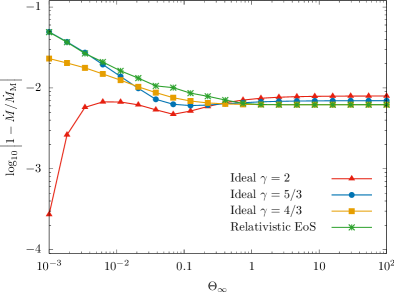
Figure 6: Relative error in the mass accretion rate between the numerical results $(\dot{M})$ and the Michel analytic solution $(\dot{M}_{\mathrm{M}})$, as a function of the asymptotic temperature $\Theta_{\text{\tiny$\infty$ }}$. We plot the results for $\gamma=4/3,5/3,2$ and the relativistic EoS.

We also perform additional numerical tests to validate the implementation of a non-zero spin parameter in our setup. In order to approximate the ultra-relativistic stiff EoS and to compare with the PST analytic solution, we perform simulations using an adiabatic index $\gamma=2$ and an asymptotic temperature $\Theta_{\text{\tiny$\infty$ }}=10^{2}$, for different values of $a$. The result of this comparison is shown in Figures 7 and 8, from where we find an excellent agreement between both solutions, with a relative error of less than 1%. We explain these two figures in further detail in the next subsection.

3.4 Results

In order to quantify the spherical accretion flow onto a rotating Kerr black hole and analyse its dependence on the black hole’s spin parameter $a$, we perform a series of simulations varying both $a$ and $\Theta_{\text{\tiny$\infty$ }}$, both for a polytrope with $\gamma=4/3,5/3,2$ as well as for the relativistic EoS.

For the spin parameter, we take a uniformly distributed set of values between $a=0$ (non-rotating black hole) and $a/M=0.99$. On the other hand, for the temperatures we choose a list of representative values between $\Theta_{\text{\tiny$\infty$ }}=10^{-3}$ and $10^{2}$, in order to study the behaviour of the solution in the transition from the non-relativistic regime to the ultra-relativistic one.

3.4.1 Temperature dependence: rotating black hole case

We explore the variation in the mass accretion rate for the rotating black hole case $a>0$, as compared with the non-rotating case. We find that the larger difference is obtained for a maximally rotating black hole, as is to be expected considering the analytic PST solution (see equation 2.49).

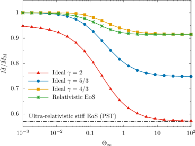
Figure 7: Mass accretion rate as a function of $\Theta_{\text{\tiny$\infty$ }}$, for a rotating black hole with $a/M=0.99$. The first three lines show the results for an ideal gas EoS with different values of $\gamma$, and the last line represents the relativistic EoS. The black dashed line represents the ultra-relativistic stiff EoS lower limit. The mass accretion rate is normalised using the corresponding value in the non-rotating case ($\dot{M}_{\rm{M}}$).

In Figure 7 we show the steady-state mass accretion rate as a function of the asymptotic temperature (for $\gamma=4/3,5/3,2$ and the relativistic EoS) for the case of a rotating black hole with a spin parameter $a/M=0.99$. The mass accretion rate is normalised by the corresponding Michel value ($a=0$). As can be seen from this figure, all simulations are bounded between the non-rotating black hole value $(\dot{M}/\dot{M}_{\rm{M}}=1)$ and the ultra-relativistic stiff EoS case $(\dot{M}/\dot{M}_{\rm{M}}\simeq 0.57)$. In the non-relativistic regime $(\Theta_{\infty}\ll 1)$, the mass accretion rate for all $\gamma$ values converges to the corresponding Michel solution, although this convergence appears to be much slower in the case $\gamma=2$. Thus, we conclude that in this regime the effects of the spin on $\dot{M}$ are negligible for $\gamma\leq 5/3$. In the ultra-relativistic regime $(\Theta_{\infty}\gg 1)$, $\dot{M}$ decreases by a factor of $\sim 10$, $25$, and $43\%$ for the solutions with $\gamma=4/3$, $5/3$, and $2$, respectively. Note how the solution for $\gamma=2$ in the $\Theta_{\text{\tiny$\infty$ }}\gg 1$ limit matches the ultra-relativistic stiff analytical value.

3.4.2 Spin dependence

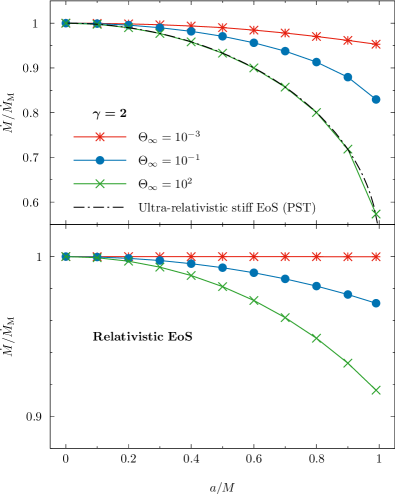
Figure 8: Mass accretion rate as a function of the spin parameter for the $\gamma=2$ (top panel) and the relativistic EoS (bottom panel), and different values of the asymptotic temperature $\Theta_{\text{\tiny$\infty$ }}$. The mass accretion rate is normalised by its value in the non-rotating case $\dot{M}_{\rm{M}}$. The black dashed line in the top panel represents the solution obtained with the ultra-relativistic stiff EoS (PST) model.

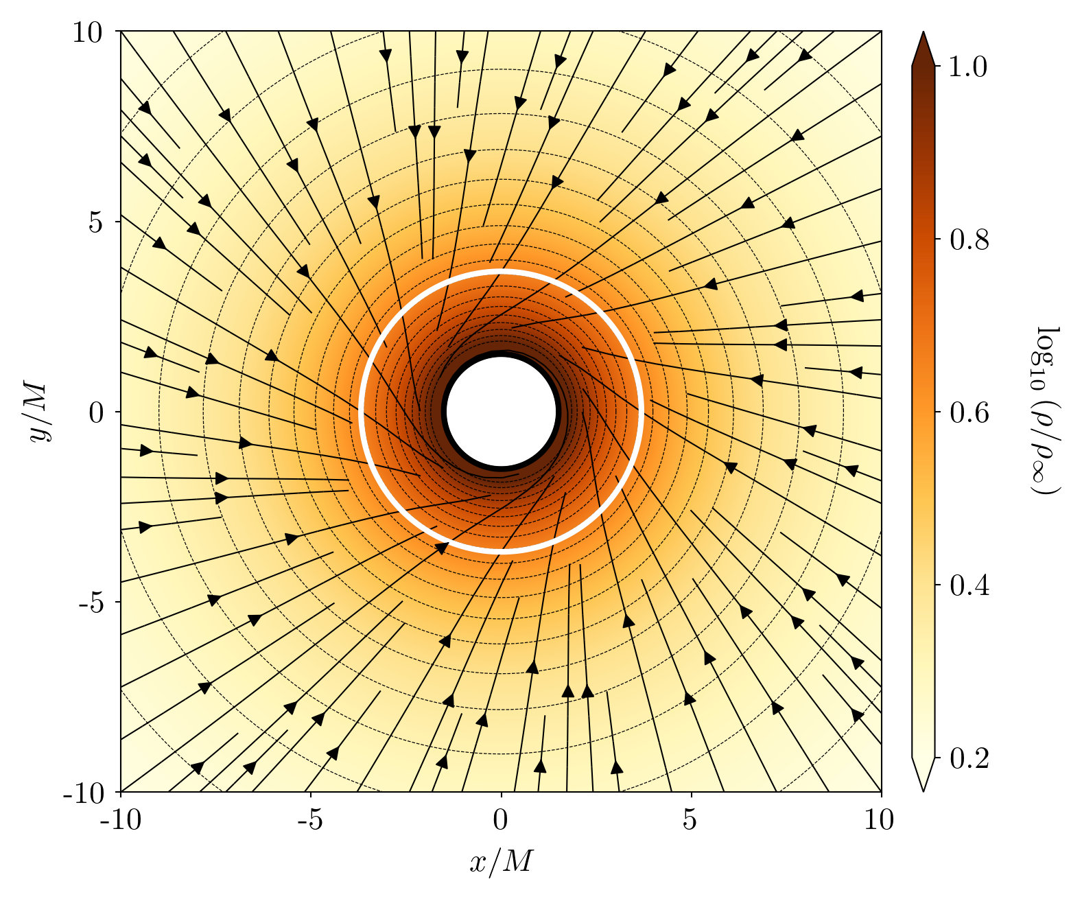
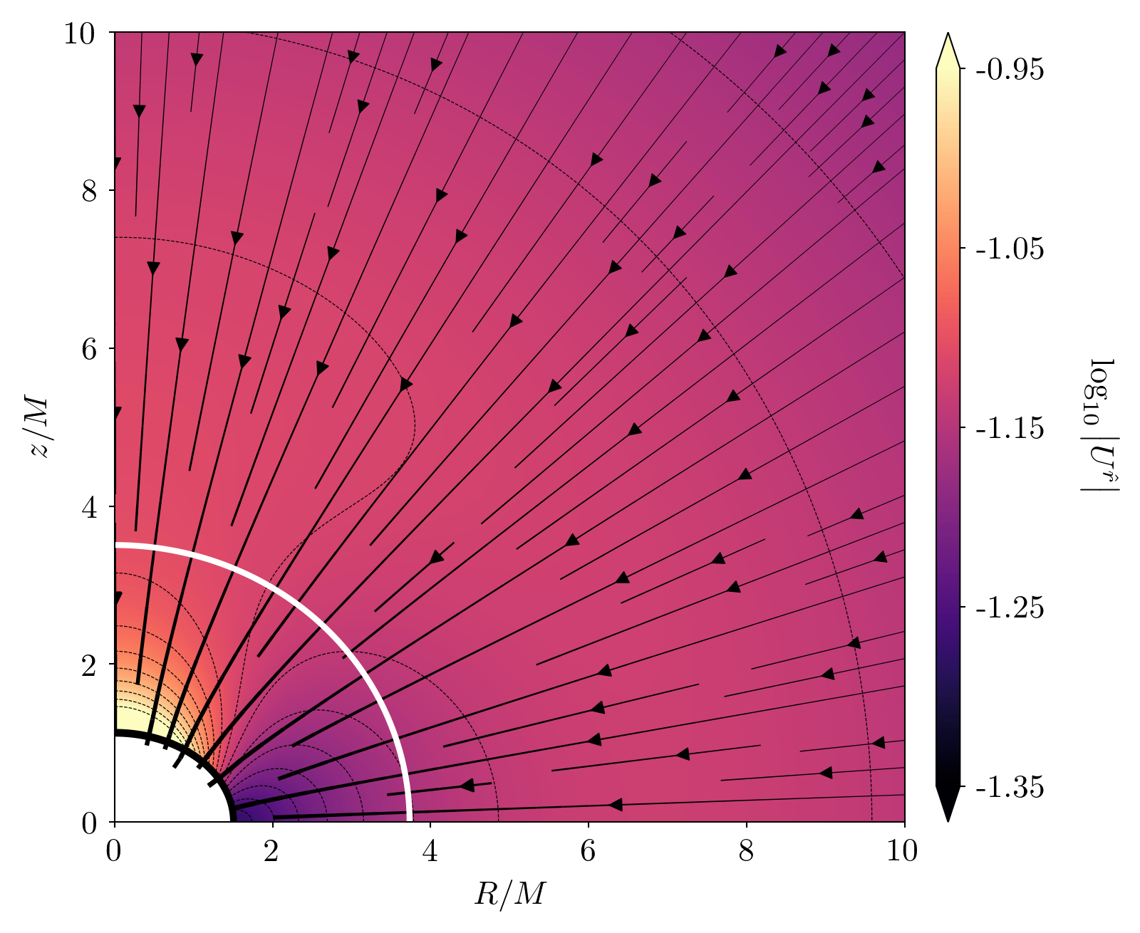
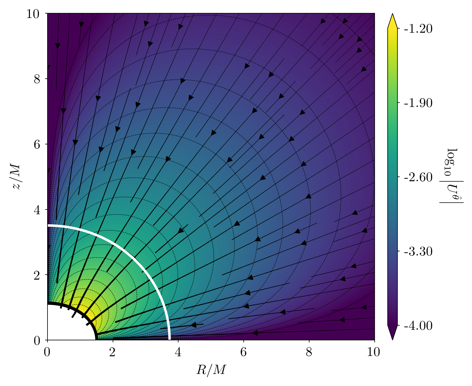
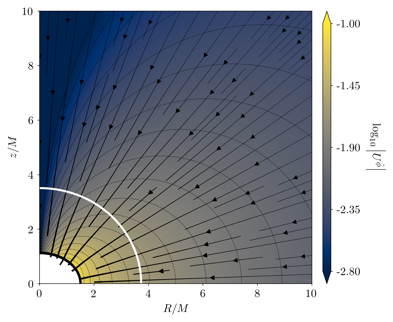
Figure 9: Isocontour plots of the steady-state of a simulation of the spherical accretion problem onto a rotating black hole with $a/M=0.99$, for a gas obeying the relativistic EoS and $\Theta_{\infty}=0.1$. The figures show the normalised rest-mass density $\rho/\rho_{\text{\tiny$\infty$ }}$ at the equatorial plane (top-left) and the spatial orthonormal components of the four-velocity ($U^{\hat{r}}$ [top-right], $U^{\hat{\theta}}$ [bottom-left] and $U^{\hat{\phi}}$ [bottom right]) projected on the $R-z$ plane, where $R=\sqrt{r^{2}+a^{2}}\,\sin\theta$ and $z=r\cos\theta$. The black solid arrows show the fluid streamlines, whereas the black dashed lines the isocontour levels. The white solid line shows the location of the sonic surface, see Figure 11 for further details. The outer boundary in this simulation is $\mathcal{R}_{\rm out}\approx 147\,M$.

In order to study the dependence of the spherical accretion solution on the spin parameter, we perform a series of simulations varying the value of $a$. For these runs, we also consider three values of the asymptotic temperature corresponding to the non-relativistic, intermediate, and ultra-relativistic regimes. In Figure 8 we show our analysis of this dependence adopting two fluid models: the stiff fluid ($\gamma=2$, top panel) and the relativistic EoS (bottom panel). The former case allows us to study the behaviour of the simulations for an extreme adiabatic index (for which the spin effects are more noticeable), while the latter constitutes a more realistic EoS. As in Figure 7, the $\gamma=2$ and $\Theta_{\text{\tiny$\infty$ }}=10^{2}$ case matches the analytic PST solution, providing yet another code validation, but now for a wide range of spin values.

As can be seen in Figure 8, the mass accretion rate decreases as the spin parameter $a$ increases. Moreover, the dependence on $a$ becomes more significant as higher temperatures are considered. In the case of the stiff fluid (top panel), we find that the mass accretion rate is reduced by up to a factor of $50\%$ for a maximally rotating black hole as compared to a non-rotating one. On the other hand, this reduction is at most of $\sim 10\%$ in the case of the relativistic EoS (bottom panel). It is interesting to note that all the numerical results follow a qualitatively similar dependence on $a$ as the analytic PST solution: the accretion rate decreasing as the spin parameter increases.

3.4.3 Global effect of the spin

The dependence on the spin parameter has been studied so far by considering only its effect on the mass accretion rate. This is important since one of the most relevant results of any accretion model is the associated mass growth of the central object. Nevertheless, it is also of interest to study the overall morphology of the resulting accretion flow in order to understand the global effect of the spin.

To study the effect of the spin on the velocity field, as well as on the rest-mass density profile, we take as a representative example one of the simulations discussed in Section 3.4.2, namely that of a fluid obeying the relativistic EoS, with an asymptotic temperature $\Theta_{\text{\tiny$\infty$ }}=0.1$, and a spin parameter $a/M=0.99$.

In Figure 9 we show the steady-state rest-mass density $\rho/\rho_{\text{\tiny$\infty$ }}$ at the equatorial plane and the spatial components of the velocity field $U^{\hat{r}}$, $U^{\hat{\theta}}$, $U^{\hat{\phi}}$ (measured in an orthonormal reference frame, see Appendix B). The solid black arrows show the fluid streamlines and the solid white line represents the location of the sonic surface (see Appendix C for its invariant determination). Note that the azimuthal flow shown in the rest-mass density and in the $U^{\hat{\phi}}$ field, is due exclusively to the frame dragging of the black hole.

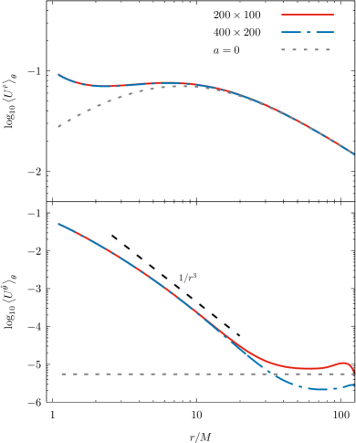
Figure 10: Solutions of the angular averaged values of $U^{\hat{r}}$ (top panel) and $U^{\hat{\theta}}$ (bottom panel) as a function of $r$, for $a/M=0.99$ and for two different resolutions. The parameters used in this plots are $\Theta_{\text{\tiny$\infty$ }}=0.1$ and the relativistic EoS. The grey dotted lines show the Michel’s $a=0$ solution in the top panel, and the average numerical error in the polar velocity in the bottom panel. Note that the difference between the two resolutions in the bottom panel for large radii is of the same order as the average numerical error. The black dashed represents the approximate behaviour of $\langle U^{\hat{\theta}}\rangle_{\theta}$.

As can be seen from Figure 9, the polar component $U^{\hat{\theta}}$ exhibits a quadrupolar-like morphology, which is in contrast to the non-rotating case where $U^{\hat{\theta}}=0$. This is interesting since in the PST solution this component of the four-velocity is exactly zero, independently of the value of the spin parameter (see equation 2.46c). On the other hand, the isocontours for $U^{\hat{r}}$ depart from spherical symmetry close to the event horizon, in particular inside the sonic surface. However, apart from the inspiraling effect due to the frame dragging, the fluid streamlines do not deviate significantly from those of the spherically symmetric inflow.

In order to analyse the behaviour of the fluid velocity, we compute the latitudinal average at each radius, defined as,

$$\left\langle U^{\hat{i}}\right\rangle_{\theta}=\frac{\displaystyle\int_{0}^{\pi/2}U^{\hat{i}}\sqrt{-g}\,\mathrm{d}\theta}{\displaystyle\int_{0}^{\pi/2}\sqrt{-g}\,\mathrm{d}\theta}.$$ (3.3)

In Figure 10 we show this average for $U^{\hat{r}}$ (upper-panel) and $U^{\hat{\theta}}$ (lower-panel) as a function of $r$ for $a/M=0.99$ and $\Theta_{\text{\tiny$\infty$ }}=0.1$. We also use two different numerical resolutions in order to show that our results are robust with respect to the grid size. The black dotted line represents the non-rotating Michel solution in the radial velocity case (top-panel), and the average numerical error that we obtain from our simulations in the polar velocity (bottom-panel). We find that the average of $U^{\hat{r}}$ is larger for a rotating black hole than for a non-rotating one. Also, in the rotating case, the average of $U^{\hat{\theta}}$ is comparable in size to $U^{\hat{r}}$ at the horizon and decreases approximately as $1/r^{3}$ for $r>r_{+}$. The fact that $U^{\hat{\theta}}$ is different from zero is relevant in view of previous work (see Shapiro, 1974; Zanotti et al., 2005), which discuss spherical accretion models in Kerr spacetime based on the assumption $U^{\theta}=0$.

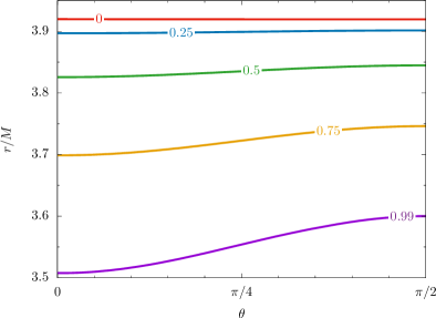
Figure 11: Resulting sonic surface as a function of the polar angle, for different values of the spin parameter $a/M$ (as indicated by the label on top of each curve). All cases correspond to the relativistic EoS with $\Theta_{\text{\tiny$\infty$ }}=0.1$. This figure shows that, for a rotating black hole, the sonic surface contracts to smaller radii and ceases to be characterised by a constant radius.

Finally, we explore in more detail the effect of the black hole spin on the sonic surface. As shown in Appendix C, this surface can be defined in an invariant way as those points at which the magnitude of the three-velocity as measured by zero angular momentum observers (ZAMOs, Bardeen, 1970) equals the local sound speed. In Figure 11 we show the shape of the sonic surface by plotting the sonic radius as a function of the polar angle, for different values of the spin parameter. As can be seen from this figure, for the non-rotating case the sonic surface corresponds to the sphere $r_{s}=\mathrm{const.}$, as expected since in this case the ZAMOs reduce to static observers. As the spin parameter increases, the sonic surface contracts unevenly giving rise to a slightly oblate shape in the $R-z$ plane. This flattening at the poles is more significant as $a/M\to 1$. For the maximum value explored in this work ($a/M=0.99$), the equator-to-poles difference in radii is of around $5\%$.

4 Summary and conclusions

In this work we have studied the spherical accretion problem from the non-relativistic regime to the ultra-relativistic one, for both rotating and non-rotating black holes. We have focused on steady-state solutions for a perfect fluid obeying an ideal gas EoS and parametrised its thermodynamic state far away from the black hole using the dimensionless temperature $\Theta_{\text{\tiny$\infty$ }}=P_{\text{\tiny$\infty$ }}/(\rho_{\text{\tiny$\infty$ }}c^{2})$. We have also assumed that the gravitational field is dominated by the black hole, such that the fluid’s self-gravity can be neglected. We first revisited the analytic solutions of Bondi (1952) and Michel (1972), and provided a quantitative comparison between them. Next, we extended Michel’s solution to the case of an ideal gas obeying a relativistic EoS (Jüttner, 1911; Synge, 1957). Finally, we studied the spherical accretion problem in the case of a rotating black hole, first by writing the exact ultra-relativistic, stiff solution (Petrich et al., 1988) in the spherically symmetric case and then by performing general relativistic hydrodynamic simulations of a general perfect fluid.

Concerning the comparison between the Bondi and Michel solutions, we have shown rigorously that Michel’s solution reduces to the Bondi one when the non-relativistic limit is considered ($\Theta_{\text{\tiny$\infty$ }}\ll 1$) and when $\gamma\leq 5/3$, as expected. Importantly, when $\gamma>5/3$, the obtained global solution is intrinsically relativistic, even for non-relativistic asymptotic temperatures, in accordance with Richards et al. (2021a). Additionally, we derived appropriate analytic expressions for the mass accretion rate for the Michel solution in the ultra-relativistic limit ($\Theta_{\infty}\gg 1)$. Moreover, within this limit and for a stiff EoS ($\gamma=2$), we have shown that the resulting mass accretion rate coincides exactly with the result obtained by Petrich et al. (1988). Furthermore, we have shown that in the isothermal limit, in which $\gamma\to 1$, the entire accretion flow can be described in a Newtonian way, i.e. the Michel solution reduces to the Bondi one for all asymptotic temperatures $\Theta_{\infty}$.

Regarding the relativistic regime, we have found that the difference between the mass accretion rates as obtained in the Bondi and Michel solutions grows arbitrarily as the asymptotic temperature increases. The reason behind this relies in the fact that, at ultra-relativistic temperatures ($\Theta_{\infty}\gg 1)$, the Michel mass accretion rate reaches a minimum constant value, whereas the Bondi one decreases without limit (Figure 4). The discrepancy between these two values is already noticeable (of order one) for $\Theta_{\infty}\sim 0.1$. Moreover, we have extended the Michel solution by considering the relativistic EoS of an ideal, monoatomic gas (Jüttner, 1911; Synge, 1957), which is a more accurate description for a perfect fluid in this regime (Figure 5).

We have also extended, by means of numerical simulations, the Michel solution to the case of a rotating Kerr black hole. The main purpose of this numerical exploration was to analyse the effect of the black hole spin on the mass accretion rate and the flow morphology. We ran a series of 2.5D general relativistic hydrodynamic simulations varying different parameters including the asymptotic temperature $\Theta_{\text{\tiny$\infty$ }}$, the gas EoS, and the spin parameter of the black hole. We have validated our results by comparing them with the known analytic solutions, as well as by performing a series of careful resolution and domain-size convergence tests.

The numerical results show that the influence of the black hole’s rotation is only larger than a few percent in the relativistic regime $(\Theta_{\text{\tiny$\infty$ }}\gtrsim 0.1)$ or for $\gamma>5/3$ (Figure 7). As the spin parameter increases, the mass accretion rate decreases as compared with the non-rotating case. This effect is stronger for larger values of $\Theta_{\text{\tiny$\infty$ }}$ and $\gamma$. Nevertheless, even in the most extreme case ($\Theta_{\infty}\gg 1$ and $\gamma=2$), the reduction in the accretion rate is no larger than $50\%$ (Figure 8). The simulations in this work allowed us to study the morphology of the fluid’s density profile and velocity field near the event horizon, showing in the latter a behaviour considerably different from the non-rotating black hole case, even for mildly relativistic temperatures. We have shown that the black hole rotation induces an azimuthal velocity component (entirely due to relativistic frame-dragging), a non-zero polar angular velocity component, as well as a non-spherically symmetric radial component (Figures 9 and 10). Furthermore, the sonic surface ceases to be characterised by a constant radial coordinate (Figure 11).

Our results imply that the relativistic features of a black hole can be safely neglected when considering the spherical accretion of a fluid with a non-relativistic asymptotic temperature ($\Theta_{\infty}\ll 1$) and $\gamma\leq 5/3$. However, this is not true for relativistic and ultra-relativistic values of the asymptotic temperature ($\Theta_{\infty}\gtrsim 0.1$). In this regime, a proper relativistic description must be used in order to compute the mass accretion rate, as the Bondi and Michel solutions lead to completely different values. On the other hand, the black hole’s rotation, even in the ultra-relativistic case and for a close-to-maximally rotating black hole, does not change the resulting mass accretion rate by more than 50% (for $\gamma\leq 2$) with respect to the non-rotating case. For a more realistic EoS ($\gamma=4/3$) this change is even smaller and lies below 10%. Thus, it is safe to neglect the black hole spin when considering an order of magnitude estimation, but it should be taken into account when performing a more accurate calculation.

The results presented in this work could be useful for studying spherical accretion onto rotating and non-rotating black holes in extreme environments where the ambient gas approaches relativistic temperatures ($\Theta_{\text{\tiny$\infty$ }}\sim 1$), or that are well approximated by a stiff EoS ($\gamma>5/3$). Examples of such scenarios might range from primordial black holes accreting during the radiation era in the early universe evolution (especially between the quark and lepton epochs when $10^{10}\leavevmode\nobreak\ \mathrm{K}<T<10^{15}\leavevmode\nobreak\ \mathrm{K}$) (Jedamzik, 1997; Lora-Clavijo et al., 2013), to mini black holes accreting from within a neutron star (whose core can be modelled, as a first approximation, with a $\gamma=2$ polytrope) (Capela et al., 2013; Génolini et al., 2020).

Data availability

All of the simulations presented in this work can be reproduced using the “Spherical accretion” setup of the aztekas code that can be found on the Github repository (https://github.com/aztekas-code/aztekas-main). Any further data underlying this paper will be shared upon request to the corresponding author.

Appendix A Limits of the Michel solution

In this appendix we make a few remarks regarding the following two limits of the Michel solution: the isothermal limit for which the adiabatic index $\gamma\to 1$ and the non-relativistic limit for which the asymptotic temperature is $\Theta_{\infty}\ll 1$.

(i) Isothermal limit

In the limit when $\gamma\to 1$, we show that the Michel solution approaches the Newtonian (Bondi) flow solution with an EoS given by equation (2.5). To this end, we first use the cubic equation (2.18) and find, for small values of $\delta:=\gamma-1>0$,

$$\frac{h_{s}}{h_{\text{\tiny$\infty$ }}}=1+\frac{3}{2}\delta-\left(\frac{9}{8}+\frac{3}{2\Theta_{\text{\tiny$\infty$ }}}\right)\delta^{2}+{\cal O}(\delta^{3}),$$ (A.4a)

$$\mathcal{C}^{2}_{\text{\tiny$\infty$ }}=\delta\left[1-\frac{\delta}{\Theta_{\text{\tiny$\infty$ }}}+{\cal O}(\delta^{2})\right],$$ (A.4b)

$$\frac{\mathcal{C}_{s}}{\mathcal{C}_{\text{\tiny$\infty$ }}}=1+{\cal O}(\delta)^{2},$$ (A.4c)

from which

$$\frac{\dot{M}_{M}}{4\pi M^{2}\rho_{\text{\tiny$\infty$ }}\mathcal{C}^{-3}_{\text{\tiny$\infty$ }}}\to\frac{1}{4}e^{3/2},$$ (A.5)

which coincides with the Bondi solution in equation (2.7).

Next, we introduce the dimensionless quantities

$$x:=\frac{r}{M}\mathcal{C}^{2}_{\text{\tiny$\infty$ }},\quad z:=\frac{\rho}{\rho_{\text{\tiny$\infty$ }}},\quad\nu:=\frac{u}{c},\quad\lambda:=\frac{\dot{M}_{M}}{4\pi M^{2}}\frac{\mathcal{C}^{3}_{\text{\tiny$\infty$ }}}{\rho_{\text{\tiny$\infty$ }}}.$$ (A.6)

in terms of which eqs. (2.14a,2.14b) can be rewritten as

$$x^{2}\nu z^{\frac{\gamma+1}{2}}=\lambda\left(\frac{h}{h_{\text{\tiny$\infty$ }}}\right)^{1/2},$$ (A.7a)

$$-\frac{2}{x}+\frac{h_{\text{\tiny$\infty$ }}}{h}z^{\gamma-1}\nu^{2}=\frac{1}{\mathcal{C}^{2}_{\text{\tiny$\infty$ }}}\left[\left(\frac{h_{\text{\tiny$\infty$ }}}{h}\right)^{2}-1\right].$$ (A.7b)

For small values of $\delta$, one finds, using $h=1+\gamma\rho^{\delta}/\delta$,

$$\frac{h}{h_{\text{\tiny$\infty$ }}}=1+\delta\log(z)+{\cal O}(\delta^{2}).$$ (A.8)

Introduced into equations (A.7a),(A.7b), using equation (A.4b) and taking the limit $\delta\to 0$ yields (assuming that $x$, $z$ and $\nu$ have finite values in this limit)

$$x^{2}\nu z=\lambda,\qquad-\frac{1}{x}+\frac{1}{2}\nu^{2}=-\log z,$$ (A.9)

which agrees precisely with the Newtonian equations (2.3a,2.3b) with the EoS (2.5), for $x$, $z$ and $\lambda$ defined as in Eq. (A.6) and $\nu=v/\mathcal{C}_{\text{\tiny$\infty$ }}$ (note that $c/\mathcal{C}_{\text{\tiny$\infty$ }}\to 1$ in the limit $\delta\to 0$). Taking into account the limit (A.5) this yields the transonic flow solution discussed in subsection 2.1 which has been shown in Ref. Chaverra & Sarbach (2016) to be the correct $\gamma\to 1$ limit of the Bondi flow.

(ii) Non-relativistic limit

In the low-temperature limit $\Theta_{\text{\tiny$\infty$ }}\to 0$ one has $h_{\text{\tiny$\infty$ }}\to 1$, and in this limit equation (2.18) has two positive roots

$$h_{s}=1,\qquad h_{s}=\frac{1}{2}\left(\sqrt{12\gamma-11}-1\right),$$ (A.10)

the third one being negative and hence unphysical. For $\gamma<5/3$ the second positive root is smaller than one, and hence unphysical as well and the correct limit is $h_{s}=1$. Computing the first-order correction in $\Theta_{\text{\tiny$\infty$ }}$ one finds

$$\frac{h_{s}}{h_{\text{\tiny$\infty$ }}}=1+\frac{3\gamma}{5-3\gamma}\Theta_{\text{\tiny$\infty$ }}+{\cal O}(\Theta_{\text{\tiny$\infty$ }})^{2},$$ (A.11)

from which

$$\frac{\mathcal{C}_{s}^{2}}{\mathcal{C}^{2}_{\text{\tiny$\infty$ }}}=\frac{2}{5-3\gamma}+{\cal O}(\Theta_{\text{\tiny$\infty$ }}),$$ (A.12)

and substituting into equation (2.22) it follows that $\dot{M}_{M}\to\dot{M}_{B}$ when $\Theta_{\text{\tiny$\infty$ }}\to 0$ and $\gamma<5/3$. When $\gamma>5/3$ it turns out the correct root is the second one in equation (A.10), see Chaverra et al. (2016), and the corresponding squared sound speed and radius at the sonic point are

$$\mathcal{C}_{s}^{2}=\frac{1}{3}(h_{s}^{2}-1)>0,\qquad r_{s}=\frac{3M}{2}\frac{h_{s}^{2}}{h_{s}^{2}-1}.$$ (A.13)

It follows from equation (2.22) that

$$\dot{M}_{M}\to\pi h_{s}^{\frac{3\gamma-2}{\gamma-1}}\mathcal{C}_{s}^{\frac{5-3\gamma}{\gamma-1}}M^{2}\rho_{\text{\tiny$\infty$ }}\,\mathcal{C}^{-\frac{2}{\gamma-1}}_{\text{\tiny$\infty$ }},$$ (A.14)

and the mass accretion rate decays slower than $\mathcal{C}^{-3}_{\text{\tiny$\infty$ }}$. Note that $h_{s}>1$ and $\mathcal{C}_{s}>0$ imply that the flow does not lie in the Newtonian regime close to the sonic point when $\gamma>5/3$.

Appendix B Orthonormal frame adapted to the Kerr-type coordinates

The orthonormal frame adapted to the constant time slices in the Kerr-type coordinates $(t,\phi,r,\theta)$ used in this article is given by

$$e_{\hat{t}} =\sqrt{1+\frac{2Mr}{\varrho^{2}}}\left(\frac{\partial}{\partial t}-\frac{2Mr}{\varrho^{2}+2Mr}\frac{\partial}{\partial r}\right),$$ (B.15a)

$$e_{\hat{r}} =\frac{1}{\sqrt{1+\frac{2Mr}{\varrho^{2}}}}\frac{\partial}{\partial r},$$ (B.15b)

$$e_{\hat{\theta}} =\frac{1}{\varrho}\frac{\partial}{\partial\theta},$$ (B.15c)

$$e_{\hat{\phi}} =\frac{1}{\varrho\sin\theta}\left(\frac{\partial}{\partial\phi}+a\sin^{2}\theta\frac{\partial}{\partial r}\right),$$ (B.15d)

and it is well-defined for all $r>0$. The corresponding components of the four-velocity vector field, such that

$$U^{\mu}\frac{\partial}{\partial x^{\mu}}=U^{\hat{t}}e_{\hat{t}}+U^{\hat{r}}e_{\hat{r}}+U^{\hat{\theta}}e_{\hat{\theta}}+U^{\hat{\phi}}e_{\hat{\phi}}$$ (B.16)

are given by

$$U^{\hat{t}} =\frac{1}{\sqrt{1+\frac{2Mr}{\varrho^{2}}}}U^{t},$$ (B.17a)

$$U^{\hat{r}} =\sqrt{1+\frac{2Mr}{\varrho^{2}}}\left(U^{r}+\frac{2Mr}{\varrho^{2}+2Mr}U^{t}-a\sin^{2}\theta U^{\phi}\right),$$ (B.17b)

$$U^{\hat{\theta}} =\varrho U^{\theta},$$ (B.17c)

$$U^{\hat{\phi}} =\varrho\sin\theta U^{\phi}.$$ (B.17d)

Appendix C Invariant determination of the sonic surface

In relativistic fluids, it is not immediately obvious how to determine the sonic surfaces, that is, the boundary separating the events at which the flow is subsonic from those at which it is supersonic. Indeed, the fluid’s sound speed $\mathcal{C}$ is a scalar, while the velocity $U^{\mu}$ of the fluid is a four-vector. One could consider instead of $U^{\mu}$ the magnitude of the three-velocity $V$ with respect to a specific family of observers and define the sonic surface by those events for which $V=\mathcal{C}$, but this definition would clearly be observer-dependent.

A definition which does provide an invariant characterization of the sonic surface is based on the sonic metric,

$$\mathfrak{G}_{\mu\nu}:=\frac{\rho}{h}\frac{1}{\mathcal{C}}\left[g_{\mu\nu}+\left(1-\mathcal{C}^{2}\right)U_{\mu}U_{\nu}\right],$$ (C.18)

first introduced by Moncrief (1980), for the purpose of analysing the propagation linearised, acoustic perturbations of an isentropic, vorticity-free flow on a background spacetime with metric $g_{\mu\nu}$. The sonic metric (C.18) is a Lorentzian metric whose set of null vectors at a given spacetime event $e$ form a cone (the sound cone) that can be shown to lie inside the light cone at $e$ provided $\mathcal{C}^{2}<1$. Another useful property of the sonic metric is that it inherits the symmetries of the spacetime and the flow configuration: if $X$ is a Killing vector field, such that the Lie derivative $\pounds_{X}$ of $g_{\mu\nu}$, $U^{\mu}$, $\rho$ and $h$ vanish, then it follows that $\pounds_{X}\mathfrak{G}_{\mu\nu}=0$, that is, the sonic metric is invariant with respect to $X$.

For the solutions described in this article, where both the spacetime metric and the flow are steady-state and axisymmetric, it follows that Eq. (C.18) describes a steady-state and axisymmetric geometry which is asymptotically flat since the flow’s four-velocity is constant at infinity. A sonic surface corresponds to the “event horizon” of this geometry, that is, the surface which separates those events that can send an acoustic signal to infinity from those that cannot. Due to the aforementioned symmetries of the sonic geometry, this surface must be a Killing horizon, i.e. a null surface of the form (see, e.g. Heusler, 1996)

$${\cal H}:=\{x:\mathfrak{G}_{\mu\nu}(x)X^{\mu}X^{\nu}=0\},$$ (C.19)

whose normal vector,

$$X^{\mu}=\delta^{\mu}{}_{t}+\Omega_{\cal H}\delta^{\mu}{}_{\phi},$$ (C.20)

is a superposition of the Killing vector fields of the Kerr metric, where here the constant $\Omega_{\cal H}$ describes the angular velocity of the horizon. The requirement of ${\cal H}$ being a null surface (with respect to the sonic metric) with normal $X^{\mu}$ implies the condition

$$\nabla^{\alpha}\left[\mathfrak{G}_{\mu\nu}(x)X^{\mu}X^{\nu}\right]=-2\kappa X^{\alpha},$$ (C.21)

the proportionality factor $\kappa$ describing the “surface gravity” associated with the horizon. Assuming a regular horizon, such that $\kappa\neq 0$, the four equations (C.21) imply

$$\mathfrak{G}_{tt}+\Omega_{\cal H}\mathfrak{G}_{t\phi}=0,$$ (C.22a)

$$\mathfrak{G}_{t\phi}+\Omega_{\cal H}\mathfrak{G}_{\phi\phi}=0,$$ (C.22b)

$$\mathfrak{G}_{tr}+\Omega_{\cal H}\mathfrak{G}_{\phi r}=-\frac{1}{2\kappa}\frac{\partial N}{\partial r},$$ (C.22c)

$$\mathfrak{G}_{t\theta}+\Omega_{\cal H}\mathfrak{G}_{\phi\theta}=-\frac{1}{2\kappa}\frac{\partial N}{\partial\theta}$$ (C.22d)

with $N:=\mathfrak{G}_{\mu\nu}X^{\mu}X^{\nu}=\mathfrak{G}_{tt}+2\Omega_{\cal H}\mathfrak{G}_{t\phi}+\Omega_{\cal H}^{2}\mathfrak{G}_{\phi\phi}$. Note that the first two conditions (C.22a,C.22b) imply that $X^{\mu}$ is null on ${\cal H}$, i.e. $N=0$, as required. They determine the location of the sonic surface ${\cal H}$ through the requirement that the determinant of the $2\times 2$ matrix $(\mathfrak{G}_{ab})_{a,b=t,\phi}$ vanishes. In view of definition (C.18) this yields

$$\det\left[g_{ab}+(1-\mathcal{C}^{2})U_{a}U_{b}\right]=0.$$ (C.23)

In turn, either Eq. (C.22c) or Eq. (C.22d) can be used to determine the surface gravity $\kappa$, but this will not be needed here.

In terms of the Kerr-type coordinates $(t,\phi,r,\theta)$ used in this article, the determinant condition (C.23), together with the property $U_{\phi}=0$ satisfied by the flow, leads to the condition

$$g_{tt}-\frac{g_{t\phi^{2}}}{g_{\phi\phi}}+(1-\mathcal{C}^{2})U_{t}^{2}=0,$$ (C.24)

which yields an implicit relation between $r$ and $\theta$. This condition acquires a much clearer interpretation when rewriting it in terms of the flow’s Lorentz factor $\Gamma$ measured by a ZAMO, which gives

$$(1-\mathcal{C}^{2})\Gamma^{2}=1,$$ (C.25)

i.e. the sonic surface is determined by those events for which the flow, as measured by ZAMOs, changes from sub- to supersonic. From Eq. (C.22b) and $U_{\phi}=0$ it also follows that $\Omega_{\cal H}=-g_{t\phi}/g_{\phi\phi}=\Omega_{\rm ZAMO}$, i.e. the angular velocity of the sonic horizon is equal to the angular velocity of the ZAMO at ${\cal H}$.

References

- Abbas & Ditta (2021) Abbas G., Ditta A., 2021, New Astron., 84, 101508
- Abramowicz & Zurek (1981) Abramowicz M. A., Zurek W. H., 1981, ApJ, 246, 314
- Aguayo-Ortiz et al. (2018) Aguayo-Ortiz A., Mendoza S., Olvera D., 2018, PLOS One, 13, e0195494
- Aguayo-Ortiz et al. (2019) Aguayo-Ortiz A., Tejeda E., Hernandez X., 2019, MNRAS, 490, 5078
- Aguayo-Ortiz et al. (2021) Aguayo-Ortiz A., Sarbach O., Tejeda E., 2021, Phys. Rev. D, 103, 023003
- Alcubierre (2008) Alcubierre M., 2008, Introduction to 3+1 Numerical Relativity. International series of monographs on physics, Oxford Univ. Press, Oxford, doi:10.1093/acprof:oso/9780199205677.001.0001
- Armitage (2020) Armitage P. J., 2020, A&G, 61, 2.40
- Banyuls et al. (1997) Banyuls F., Font J. A., Ibáñez J. M., Martí J. M., Miralles J. A., 1997, ApJ, 476, 221
- Bardeen (1970) Bardeen J. M., 1970, ApJ, 162, 71
- Begelman (1978) Begelman M. C., 1978, MNRAS, 184, 53
- Beskin & Pidoprygora (1995) Beskin V. S., Pidoprygora Y. N., 1995, J. Exp. Theor. Phys., 80, 575
- Bondi (1952) Bondi H., 1952, MNRAS, 112, 195
- Capela et al. (2013) Capela F., Pshirkov M., Tinyakov P., 2013, Phys. Rev. D, 87, 123524
- Carr (1981) Carr B. J., 1981, MNRAS, 194, 639
- Carroll (2003) Carroll S., 2003, Spacetime and Geometry: An Introduction to General Relativity. Benjamin Cummings, doi:https://doi.org/10.1017/9781108770385
- Chaverra & Sarbach (2015) Chaverra E., Sarbach O., 2015, Class. Quantum Grav., 32, 155006
- Chaverra & Sarbach (2016) Chaverra E., Sarbach O., 2016, Gen. Relativ. Gravit., 48, 12
- Chaverra et al. (2016) Chaverra E., Mach P., Sarbach O., 2016, Class. Quantum Grav., 33, 105016
- Chavez Nambo & Sarbach (2020) Chavez Nambo E., Sarbach O., 2020, Static spherical perfect fluid stars with finite radius in general relativity: a review (arXiv:2010.02859)
- Cieślik & Mach (2020) Cieślik A., Mach P., 2020, Phys. Rev. D, 102, 024032
- Ciotti & Pellegrini (2017) Ciotti L., Pellegrini S., 2017, ApJ, 848, 29
- Colpi et al. (1996) Colpi M., Shapiro S. L., Wasserman I., 1996, ApJ, 470, 1075
- Davé et al. (2019) Davé R., Anglés-Alcázar D., Narayanan D., Li Q., Rafieferantsoa M. H., Appleby S., 2019, MNRAS, 486, 2827
- Del Zanna et al. (2007) Del Zanna L., Zanotti O., Bucciantini N., Londrillo P., 2007, A&A, 473, 11
- Falle & Komissarov (1996) Falle S. A. E. G., Komissarov S. S., 1996, MNRAS, 278, 586
- Génolini et al. (2020) Génolini Y., Serpico P. D., Tinyakov P., 2020, Phys. Rev. D, 102, 083004
- Heusler (1996) Heusler M., 1996, Black Hole Uniqueness Theorems. Cambridge University Press, Cambridge, England, doi:https://doi.org/10.1017/CBO9780511661396
- Igumenshchev & Narayan (2002) Igumenshchev I. V., Narayan R., 2002, ApJ, 566, 137
- Jedamzik (1997) Jedamzik K., 1997, Phys. Rev. D, 55, R5871
- Jüttner (1911) Jüttner F., 1911, in Das Maxwellsche Gesetz der Geschwindigkeitsverteilung in der Relativtheorie. Ann. Phys., pp 856–882, doi:https://doi.org/10.1002/andp.19113390503
- Karkowski & Malec (2013) Karkowski J., Malec E., 2013, Phys. Rev. D, 87, 044007
- Kouvaris & Tinyakov (2014) Kouvaris C., Tinyakov P., 2014, Phys. Rev. D, 90, 043512
- Krolik & London (1983) Krolik J. H., London R. A., 1983, ApJ, 267, 18
- Krumholz et al. (2005) Krumholz M. R., McKee C. F., Klein R. I., 2005, ApJ, 618, 757
- Lora-Clavijo et al. (2013) Lora-Clavijo F. D., Guzmán F. S., Cruz-Osorio A., 2013, J. Cosmol. Astropart. Phys., 2013, 015
- Mach et al. (2018) Mach P., Piróg M., Font J. A., 2018, Class. Quantum Grav., 35, 095005
- Malec (1999) Malec E., 1999, Phys. Rev. D, 60, 104043
- Maraschi et al. (1974) Maraschi L., Reina C., Treves A., 1974, A&A, 35, 389
- McKinney et al. (2014) McKinney J. C., Tchekhovskoy A., Sadowski A., Narayan R., 2014, MNRAS, 441, 3177
- Michel (1972) Michel F. C., 1972, Ap&SS, 15, 153
- Miller & Baumgarte (2017) Miller A. J., Baumgarte T. W., 2017, Class. Quantum Grav., 34, 035007
- Moffat (2020) Moffat J. W., 2020, Supermassive Black Hole Accretion and Growth (arXiv:2011.13440)
- Moncrief (1980) Moncrief V., 1980, ApJ, 235, 1038
- Moscibrodzka (2006) Moscibrodzka M., 2006, A&A, 450, 93
- Narayan et al. (2019) Narayan R., Johnson M. D., Gammie C. F., 2019, ApJL, 885, L33
- Pariev (1996) Pariev V. I., 1996, MNRAS, 283, 1264
- Petrich et al. (1988) Petrich L. I., Shapiro S. L., Teukolsky S. A., 1988, Phys. Rev. Lett., 60, 1781
- Proga & Begelman (2003) Proga D., Begelman M. C., 2003, ApJ, 582, 69
- Ressler et al. (2021) Ressler S. M., Quataert E., White C. J., Blaes O., 2021, MNRAS,
- Richards et al. (2021a) Richards C. B., Baumgarte T. W., Shapiro S. L., 2021a, arXiv e-prints, p. arXiv:2101.08797
- Richards et al. (2021b) Richards C. B., Baumgarte T. W., Shapiro S. L., 2021b, arXiv e-prints, p. arXiv:2102.09574
- Rioseco & Sarbach (2017a) Rioseco P., Sarbach O., 2017a, Class. Quantum Grav., 34, 095007
- Rioseco & Sarbach (2017b) Rioseco P., Sarbach O., 2017b, in Journal of Physics Conference Series. p. 012009 (arXiv:1701.07104), doi:10.1088/1742-6596/831/1/012009
- Russell et al. (2013) Russell H. R., McNamara B. R., Edge A. C., Hogan M. T., Main R. A., Vantyghem A. N., 2013, MNRAS, 432, 530
- Russell et al. (2015) Russell H. R., Fabian A. C., McNamara B. R., Broderick A. E., 2015, MNRAS, 451, 588
- Ryu et al. (2006) Ryu D., Chattopadhyay I., Choi E., 2006, ApJS, 166, 410
- Shapiro (1974) Shapiro S. L., 1974, ApJ, 189, 343
- Sharma et al. (2008) Sharma P., Quataert E., Stone J. M., 2008, MNRAS, 389, 1815
- Shu & Osher (1988) Shu C.-W., Osher S., 1988, J. Comput. Phys., 77, 439
- Synge (1957) Synge J., 1957, The Relativistic Gas. North-Holland, Amsterdam, doi:https://doi.org/10.1063/1.3062345
- Taub (1948) Taub A. H., 1948, Phys. Rev., 74, 328
- Tejeda (2018) Tejeda E., 2018, Rev. Mex. Astron. Astrofis., 54, 171
- Tejeda & Aguayo-Ortiz (2019) Tejeda E., Aguayo-Ortiz A., 2019, MNRAS, p. 1445
- Tejeda et al. (2020) Tejeda E., Aguayo-Ortiz A., Hernandez X., 2020, ApJ, 893, 81
- Toropin et al. (1999) Toropin Y. M., Toropina O. D., Savelyev V. V., Romanova M. M., Chechetkin V. M., Lovelace R. V. E., 1999, ApJ, 517, 906
- Weih et al. (2020) Weih L. R., Olivares H., Rezzolla L., 2020, MNRAS, 495, 2285
- Yang et al. (2021) Yang S., Liu C., Zhu T., Zhao L., Wu Q., Yang K., Jamil M., 2021, Chin. Phys. C, 45, 015102
- Zanotti et al. (2005) Zanotti O., Font J. A., Rezzolla L., Montero P. J., 2005, MNRAS, 356, 1371
- Zel’dovich & Novikov (1967) Zel’dovich Y. B., Novikov I. D., 1967, Soviet Ast., 10, 602