Dissecting the Inner Galaxy with $\gamma$-Ray Pixel Count Statistics

Abstract

We combine adaptive template fitting and pixel count statistics in order to assess the nature of the Galactic center excess in Fermi-LAT data. We reconstruct the flux distribution of point sources well below the Fermi-LAT detection threshold, and measure their radial and longitudinal profiles in the inner Galaxy. We find that all point sources $and$ the bulge-correlated diffuse emission each contributes $\mathcal{O}$(10%) of the total inner Galaxy emission, and disclose a potential sub-threshold point-source contribution to the Galactic center excess.

Introduction. The Galactic center excess (GCE) shows up as an unexpected $\gamma$-ray component in the data of the Large Area Telescope (LAT), aboard the Fermi satellite, at GeV energies, from the inner degrees of the Galaxy Abazajian and Kaplinghat (2012); Gordon and Macias (2013); Calore et al. (2015a); Daylan et al. (2016); Ajello et al. (2016). Despite the great interest raised by the GCE discovery, its nature is still unknown. While the GCE morphology has been found to be consistent with a Navarro, Frenk and White (NFW) profile Navarro et al. (1997) for annihilating particle dark matter (DM) in Abazajian and Kaplinghat (2012); Daylan et al. (2016); Calore et al. (2015b); Agrawal et al. (2015); Murgia (2020); Di Mauro (2021), it could also be due to a population of millisecond pulsars, as proposed by Abazajian (2011). Stellar distributions were used as tracers of point sources (PS) emitting below threshold, and turned out to match the morphological features of GCE photons better than DM-inspired templates in Bartels et al. (2018); Macias et al. (2018, 2019). All these results were obtained by $\gamma$-ray analyses based on the, so-called, template fitting. In parallel, complementary methods, based on photon-count statistics and aimed at detecting new point sources below the threshold of the Fermi catalogs were developed. They initially revealed that the GCE can be entirely due to a population of PS Bartels et al. (2016); Lee et al. (2016). More recently, the DM interpretation was brought back by Leane and Slatyer (2019), although hampered by systematics affecting photon-count statistical methods Leane and Slatyer (2020a); Chang et al. (2020); Buschmann et al. (2020); Zhong et al. (2020); Leane and Slatyer (2020b). Techniques involving neural networks have also been explored Caron et al. (2018); List et al. (2020). As a conclusive probe of the PS nature of the GCE, a fully multiwavelength approach has been proposed, from radio to gravitational wave observations Calore et al. (2016, 2019); Berteaud et al. (2020). A major limitation to all these studies is the modeling of the Galactic diffuse foreground, and the impact of residual mis-modeled emission on the results’ robustness. As for template fitting methods, the analysis of the diffuse emission has been recently approached with the skyFACT algorithm, which fits the $\gamma$-ray sky by combining methods of image reconstruction and adaptive spatio-spectral template regression Storm et al. (2017). The skyFACT method has been tested in the Inner Galaxy (IG) region, and probed to be efficient in the removal of most residual emission for a robust assessment of the GCE properties Storm et al. (2017); Bartels et al. (2018). Another source of uncertainty is the contribution of sub-threshold PSs. Photon-count statistical methods can discriminate photons from $\gamma$-ray sources based on their statistical properties Malyshev and Hogg (2011). In particular, the 1-point probability distribution function method Zechlin et al. (2016a) (1pPDF) fits the contribution of diffuse and PS components to the $\gamma$-ray 1-point fluctuations histogram. Employing 1pPDF on Fermi-LAT data, it was possible to measure the PS count distribution per unit flux, $dN/dS$, below the LAT detection threshold at high latitudes Zechlin et al. (2016a, b); Manconi et al. (2020), and to set competitive bounds on DM Zechlin et al. (2018).

The scope of this Letter is to apply the 1pPDF method to Fermi-LAT data from the IG to understand the role of faint PS to the GCE, while minimizing the mis-modelling of diffuse emission components. To this end, we adopt a hybrid approach which combines, for the first time, adaptive template fitting methods as implemented in skyFACT, and 1pPDF techniques.

Rationale, data and methodology. We follow a two-step procedure: First, we fit $\gamma$-ray data with skyFACT in order to build a model for the emission in the region of interest (ROI), maximally reducing residuals found to bias photon-count statistical methods Buschmann et al. (2020). Secondly, we run 1pPDF fits with skyFACT-optimized diffuse models as input, and assess the role of PS to the GCE.

We analyze 639 weeks of P8R3 ULTRACLEANVETO Fermi-LAT data fer until 2020-08-27. For the skyFACT fit, we consider an ROI of 40${}^{\circ}\times 40^{\circ}$ around the GC SFf , and the $0.3-300$ GeV energy range. We closely follow Bartels et al. (2018) and update the analysis for the increased data set and 4FGL catalog Abdollahi et al. (2020). The emission model includes $\gamma$ rays from inverse Compton scattering, $\pi^{0}$ decay, 4FGL point-like and extended sources, the Fermi bubbles, the isotropic $\gamma$-ray background (IGRB), and the GCE. For the latter, we consider a template for the Galactic bulge emission as in Bartels et al. (2018), and one for a generalized NFW DM distribution with slope 1.26 (NFW126) Calore et al. (2015a); Daylan et al. (2016). We refer to sup for more details.

We operate the 1pPDF analysis in the energy range $2-5$ GeV Zechlin et al. (2016b, 2018), restricting to events with best angular reconstruction (evtype=PSF3) and coming from the inner $20^{\circ}\times 20^{\circ}$, IG ROI hereafter. We cut at latitudes $|b|>0.5^{\circ}$ or $2^{\circ}$ to check the stability of 1pPDF results. The 1pPDF-fit model components are: An IGRB template (free normalization), a diffuse emission template (free normalization), and an isotropic PS (IPS)spa population with $dN/dS$ defined by a multiple broken power law:

$$\frac{\mathrm{d}N}{\mathrm{d}S}=A_{\rm S}\cdot\begin{cases}\left(\frac{S}{S_{0}}\right)^{-n_{1}}\;\;\;\;S>S_{\mathrm{b}1}\,;\\ \left(\frac{S_{\mathrm{b}1}}{S_{0}}\right)^{-n_{1}+n_{2}}\left(\frac{S}{S_{0}}\right)^{-n_{2}}\;\;\;\;S_{\mathrm{b}2}<S\leq S_{\mathrm{b}1}\,;\\ \mathmakebox[\widthof{{}\left(\frac{S_{\mathrm{b}1}}{S_{0}}\right){}}][c]{\vdots}&\\ \left(\frac{S_{\mathrm{b}1}}{S_{0}}\right)^{-n_{1}+n_{2}}\left(\frac{S_{\mathrm{b}2}}{S_{0}}\right)^{-n_{2}+n_{3}}\cdots\ \left(\frac{S}{S_{0}}\right)^{-n_{N_{\mathrm{b}}+1}}\\ \hskip 108.12054ptS\leq S_{\mathrm{b}N_{\mathrm{b}}}.\\ \end{cases}$$ (1)

The free parameters are $A_{\rm S}$, the flux break positions, and the broken power-law indices, $n_{i}$ sup . The IPS $dN/dS$ measured by the 1pPDF fit should recover the $dN/dS$ of Fermi-LAT detected PS in the bright regime while pushing the PS detection threshold down to lower fluxes Zechlin et al. (2016a, b).

Our goal being to quantify the role of PS to the GCE within the 1pPDF, we add a GCE smooth template in the 1pPDF fit. As a baseline, we use the best-fit skyFACT bulge template in the 1pPDF fit (1pPDF-B), and we define the sF-B diffuse model as the sum of best-fit inverse Compton, $\pi^{0}$ decay, Fermi bubbles, and extended sources, thus subtracting the bulge emission. The normalization, A_B/NFW126 for the bulge/NFW126 template, refers to the rescaling factor relative to the best-fit normalization from skyFACT.

On the one hand, the use of skyFACT best-fit diffuse model guarantees a robust characterization of GCE spectrum and morphology against systematics related to the mis-modeling of the diffuse emission Buschmann et al. (2020); Calore et al. (2015a), resolving over/under-subtraction issues by including a large number of nuisance parameters. The limitations of such a systematic uncertainty are indeed also relevant for the reconstruction of faint PS with 1pPDF methods sup . On the other hand, the skyFACT optimization procedure mitigates possible systematics related to the mis-modeling of unaccounted components Leane and Slatyer (2020a), by allowing spatial re-modulation in the fit templates. Also, we stress that this is the first time the stellar distribution in the Galactic bulge as tracer of GCE photons is used in pixel count statistical analyses (except for brief cross-checks, as in e.g. Leane and Slatyer (2019)).

Besides the bulge, we also consider NFW126 as smooth GCE in the 1pPDF analysis (1pPDF-NFW126). In this case, we construct the corresponding skyFACT-optimized diffuse model (sF-NFW126) from the skyFACT run adopting NFW126 as GCE, in analogy with the sF-B model. Such a procedure guarantees maximal consistency between GCE and diffuse models adopted as input in the 1pPDF. Finally, to bracket the uncertainties related to the optimization of the diffuse model, we also build a skyFACT-optimized diffuse template from the skyFACT run not including any GCE additional template (sF-noGCE).

Results. Our updated analysis of Fermi-LAT data with skyFACT confirms previous findings from Bartels et al. (2018); Macias et al. (2018, 2019). A bulge distribution for GCE photons is strongly preferred by data on top of the NFW126-only model ($\sim 10\sigma$), and there is mild evidence for an additional NFW126 contribution on top of the bulge-only model ($\sim 4\sigma$), cf. sup . This implies that the model maximally reducing the residuals is the skyFACT best-fit of the run with the bulge.

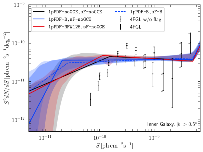
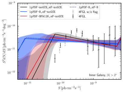
Figure 1: IPS source count distribution in the IG ROI from the 1pPDF fit for $|b|>0.5^{\circ}$ (left) or 2^∘ (right). Solid (dashed) lines correspond to sF-noGCE (sF-B) diffuse template. The black line illustrates the 1pPDF-noGCE  case. The blue (red) line refers to 1pPDF-B  (1pPDF-NFW126) case. The colored areas correspond to $1\sigma$ uncertainty bands. The black (gray) points represent the count distribution of 4FGL sources (without any analysis flag, see Abdollahi et al. (2020)).

We then use skyFACT-optimized diffuse and smooth GCE templates as input for 1pPDF fits, testing 0.5^∘ and 2^∘ latitude cuts. Our results are summarized in Fig. 1, where we show the best-fit $dN/dS$ for the IPS in the IG ROI for several 1pPDF fit configurations. First, we notice that whatever GCE template is added to the 1pPDF fit components (bulge or NFW126), its normalization never converges toward the lower bound of its prior interval, regardless of the skyFACT diffuse template adopted. The same is valid for the IPS normalization. In all fit setups shown, an IPS population is recovered below the LAT flux threshold. The reconstructed IPS $dN/dS$ is stable against systematics related to the choice of skyFACT-optimized diffuse template, and latitude cut. Moreover, it does not present any spurious effect at the Fermi-LAT threshold ($\sim 10^{-10}$ ph cm^-2 s^-1), and IPS are resolved down to $\sim 10^{-11}$ ph cm^-2 s^-1 for $|b|>0.5^{\circ}$, depending on the modeling of the smooth GCE component. This holds true even when no GCE smooth template is included neither in the skyFACT fit nor in the 1pPDF one, contrary to what happens using non-optimized diffuse models Leane and Slatyer (2020a); Buschmann et al. (2020). We therefore demonstrate, also in the context of 1pPDF methods, that reducing large-scale residuals from mis-modeling of the diffuse emission improves the reconstruction of PS $dN/dS$ (see also sup ). The reconstructed $dN/dS$ has a normalization decreasing with increasing latitude cuts, suggesting that PS are more numerous towards the very GC. When an NFW126 template is included in the 1pPDF fit, the IPS $dN/dS$ is compatible with the 1pPDF-noGCE case. In both cases, the second break in the $dN/dS$ – in addition to the one set in the bright regime – is recovered close to the LAT flux threshold. Instead, the 1pPDF-B reconstructs PS down to lower fluxes, regardless of sF-noGCE or sF-B diffuse models. For these setups, the second flux break is found at $\sim 2\cdot 10^{-11}\,(8\cdot 10^{-12})$ ph cm^-2 s^-1 for $|b|>0.5^{\circ}\,(2^{\circ})$. Going from $|b|>0.5^{\circ}$ to $|b|>2^{\circ}$, the $dN/dS$ is resolved down to even lower fluxes. A posteriori, we associate such a better sensitivity to IPS to the ability of the fitted diffuse components to further reduce fit residuals.

Table 1: Results for the 1pPDF analysis of the IG LAT data. First four columns: setup of the analysis and latitude mask of the IG. The $\ln(\mathcal{Z})$ is the nested sampling global log-evidence extracted from Multinest Zechlin et al. (2016a). Last two columns: flux percentage of different model components with respect to the total emission in the ROI (for $S<10^{-8}$ ph cm^-2 s^-1 , see sup ), and normalization of smooth GCE template in the 1pPDF. Flux percentage always sum to unity within errors.

Description	1pPDF setup	skyFACT diffuse	$|b|$ cut [∘]	$\ln(\mathcal{Z})$	Point sources/diffuse/GCE %	$A_{\rm B/NFW126}$
No GCE (both)	1pPDF-noGCE	sF-noGCE	2	$-6113$	$12/89/-$	-
Bulge (1pPDF only)	1pPDF-B	sF-noGCE	2	$-6076$	$13/81/7$	$0.8\pm 0.1$
DM (1pPDF only)	1pPDF-NFW126	sF-noGCE	2	$-6084$	$10/84/6$	$1.8^{+0.4}_{-0.2}$
Bulge (skyFACT only)	1pPDF-noGCE	sF-B	2	$-6169$	$11/89/-$	-
Bulge (both)	1pPDF-B	sF-B	2	$-6074$	$13/77/10$	$1.1\pm 0.1$
DM (both)	1pPDF-NFW126	sF-NFW126	2	$-6084$	$11/82/7$	$2.3\pm 0.3$
No GCE (both)	1pPDF-noGCE	sF-noGCE	0.5	$-7822$	$13/86/-$	-
Bulge (1pPDF only)	1pPDF-B	sF-noGCE	0.5	$-7802$	$14/83/3$	$0.3\pm 0.1$
DM (1pPDF only)	1pPDF-NFW126	sF-noGCE	0.5	$-7818$	$14/85/1$	$0.3\pm 0.1$
Bulge (skyFACT only)	1pPDF-noGCE	sF-B	0.5	$-7907$	$15/85/-$	-
Bulge (both)	1pPDF-B	sF-B	0.5	$-7796$	$14/79/7$	$0.8\pm 0.1$
DM (both)	1pPDF-NFW126	sF-NFW126	0.5	$-7820$	$14/84/2$	$0.6\pm 0.2$

We quantify now the evidence for models with an additional smooth GCE template. To this end, we compare the global evidence, $\ln\mathcal{Z}$, for the 1pPDF-noGCE, 1pPDF-B and 1pPDF-NFW126 setups, with different skyFACT diffuse model inputs. For each model combination, we compute the Bayes factor between model $i$ and $j$, $B_{ij}=\exp(\ln\mathcal{Z}_{i}-\ln\mathcal{Z}_{j})$, and assess the strength of evidence of model $i$ with respect to model $j$. Our results are presented in Tab. 1. Regardless of the skyFACT-optimized diffuse template adopted, data always more strongly support models which include an additional smooth template for the bulge with respect to models without GCE in the skyFACT and/or 1pPDF fits ($\ln B_{ij}>20$), and models with an additional smooth NFW126 component in the skyFACT and/or 1pPDF fits ($\ln B_{ij}>7$). Whenever a bulge template is included in our analysis, this is preferred even with respect to additional smooth DM templates. As for our baseline model, sF-B, and $|b|>2^{\circ}$, the evidence for an additional bulge template (1pPDF-B), with respect to 1pPDF-noGCE is $\ln B\sim 95$. Moreover, in this case the normalization of the bulge template is $A_{\rm B}=1.1\pm 0.1$, supporting the consistency between GCE and diffuse model adopted. This evidence is as strong also for $|b|>0.5^{\circ}$, $\ln B\sim 110$.

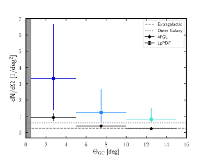
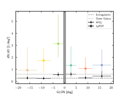
Figure 2: Radial (left) and longitude (right) source density $dN/d\Omega$ profiles, as reconstructed by the 1pPDF-B fit using the sF-B diffuse model. We also display source density profiles for 4FGL sources (black points), and average source densities in the OG and EG ROIs.

We note that, when we use the sF-noGCE diffuse model in the 1pPDF fit including the bulge (1pPDF-B), we find comparable evidence to the 1pPDF-B, sF-B setup. Indeed, skyFACT is able to re-absorb part of the photons from the bulge by re-modulating (spatially) other diffuse templates, and so, partially reduces the residuals also in the sF-noGCE case. This is perfectly consistent with the fact that $A_{\rm B}=0.8\pm 0.1$. Models with PS and a smooth bulge component are therefore strongly preferred by data, regardless of the optimized diffuse model employed. On the contrary, the evidence for an additional smooth NFW126 template with respect to models without GCE in the skyFACT fit and/or 1pPDF fits depends on the choice of the skyFACT-optimized diffuse template adopted, as well as on the latitude cut.

We have tested our results against a number of systematic effects, which are detailed in sup .

The flux percentages reported in Tab. 1 illustrate that 1pPDF fits to Fermi-LAT data find non-null (and even comparable) emission from both the IPS population $and$ the smooth GCE template, in most cases each contributing about 10% of the total emission in the ROI. Since 4FGL sources ($2^{\circ}$ cut, without analysis flag, see Fig. 1) account for 7% (10% including flagged sources) of the total IG emission, the remaining flux comes from sub-threshold IPS. We have verified sup that our results are not driven by PS in the ultra-faint regime Chang et al. (2020), where the sensitivity of the 1pPDF method drops (as quantified by the magnitude of uncertainty bands in Fig. 1), and an IPS population may become degenerate with a truly diffuse emission.

We also measure the IPS dN/dS in two control regions: The outer Galaxy (OG, $|b|<20^{\circ}$, $60^{\circ}<|l|<90^{\circ}$) and the extragalactic region (EG, $|b|>40^{\circ}$, $|l|>90^{\circ}$). The reconstructed $dN/dS$ in both OG and EG ROIs does not present any spurious threshold effect and can identify IPS down to the statistical limit of the method around $\sim 10^{-11}$ ph cm^-2 s^-1 Zechlin et al. (2016a). We compute the source density $dN/d\Omega$ in the flux interval [$10^{-11}-10^{-9}$] ph cm^-2 s^-1, finding $\sim 0.6$ sources/deg² in the OG, and $\sim 0.3$ sources/deg² in the EG, see Fig. 2.

Since the spatial distribution of PS is isotropic by construction, we test the PS spatial behavior by dissecting the IG ROI into three concentric annuli, masked for latitudes $|b|<0.5^{\circ}$. We extract the $dN/dS$ separately in each ring, and integrate it over the flux interval [$10^{-11}-10^{-9}$] ph cm^-2 s^-1. The result is reported in Fig. 2 as a function of the mean $\Theta_{\rm GC}=\sqrt{b^{2}+l^{2}}$ in each ring, for our baseline 1pPDF-B, sF-B setup. We observe a decreasing trend of the $dN/d\Omega$ in the IG with $\Theta_{\rm GC}$. Also, the $dN/d\Omega$ in the innermost ring is about a factor of three higher than 4FGL sources, as well as than in OG and EG. For the most external ring, the source density is instead comparable with the catalog, OG and EG ones. This corroborates the evidence that the IG PS population is not purely isotropic nor extragalactic in origin, but rather it peaks towards the GC. Similarly, we build the longitude profile of IG PS, Fig. 2. The $dN/dS$ has been fitted in 6 longitude slices from the GC bound at $|l|=6^{\circ},12^{\circ}$ and $20^{\circ}$. The derived $dN/d\Omega$ shows again a distribution peaked around the GC, and compatible with OG (and partially with 4FGL and EG) sources only in the most external longitude interval. This result adds a piece of evidence that the GCE (defined as an excess of photons above traditionally adopted foreground/background astrophysical models) is contributed by faint PS on lines-of-sight toward the Galactic center, and, perhaps, in the Galactic bulge, supporting their Galactic origin.

Conclusions. For the first time, we analyzed the IG Fermi-LAT sky by means of the 1pPDF photon-count statistics technique in order to understand the role of PS to the GCE. To minimize the systematic effects inherent the modeling of the $\gamma$-ray sky, we introduced important methodological novelties. First, we implemented within the 1pPDF new, optimized, models for the diffuse emission from skyFACT adaptive template fits, developing a self-consistent procedure which effectively reduces diffuse mis-modeling. Secondly, besides PS, in the 1pPDF fit we included an additional smooth GCE template which traces the stellar distribution in the Galactic bulge.

The updated skyFACT analysis of the IG confirms that the GCE is better described by a bulge template than an NFW126 model at high significance. Moreover, we find that the 1pPDF method, supplied with skyFACT diffuse emission templates, always recovers an IPS population well below the Fermi-LAT flux threshold, down to $\sim 10^{-11}$ ph cm^-2 s^-1 for $|b|>0.5^{\circ}$. The reconstructed IPS $dN/dS$ is stable against a number of systematics, in particular related to the choice of skyFACT-optimized diffuse template and latitude cut. Regardless of the skyFACT-optimized diffuse template, data always prefer models which include an additional smooth template for the bulge with respect to both models without it and models with an additional NFW126 template, in the skyFACT and/or 1pPDF fits.

Our results show that, within the statistical validity of the 1pPDF and the setups tested, IPS and diffuse bulge each contributes about $\mathcal{O}$(10%) to the $\gamma$-ray emission along the lines-of-sight toward the GC. In particular, within our baseline model the 1pPDF founds that PS (bulge) contribute 13% (10%) of the total emission of the IG. Subtracting the contribution from cataloged sources, a non-negligible fraction of the IG emission is accounted by sub-threshold PS. This further corroborates a possible, at least partial, stellar origin of the GCE.

We also verified that this IPS population is not purely isotropic nor extragalactic in origin, rather it peaks towards the very GC. Although the final confirmation of the PS nature of the GCE will most likely come from multiwavelength future observations, we undoubtedly got one step closer to the understanding of the mysterious nature of the GCE emission.

Acknowledgments. We very kindly acknowledge the work formerly done by H.S. Zechlin on the 1pPDF code. We warmly thank P. D. Serpico for inspiring discussion. We also thank M. Di Mauro, F. Kahlhoefer, M. Kraemer, P. D. Serpico, and C. Weniger for a careful reading of the manuscript and for insightful comments. The work of F.D. has been supported by the “Departments of Excellence 2018 - 2022” Grant awarded by the Italian Ministry of Education, University and Research (MIUR) (L. 232/2016). F.C. acknowledges support by the Programme National Hautes Energies (PNHE) through the AO INSU 2019, grant “DMSubG”, and the Agence Nationale de la Recherche AAPG2019, project “GECO”. S.M. acknowledges computing resources granted by RWTH Aachen University under project rwth0578.

Supplemental Material:
Dissecting the Inner Galaxy with $\gamma$-Ray Pixel Count Statistics
F.Calore, F.Donato, and S.Manconi

S1 The skyFACT analysis

In this section, we discuss in more detail the analysis and results of the Fermi-LAT $\gamma$-ray fit with skyFACT Storm et al. (2017).

For the skyFACT analysis, we consider all FRONT+BACK events (evtype=3) to maximize the statistics against the large number of free parameters in the fit. The data are binned in energy into 30 logarithmically-spaced bins from 0.2 to 500 GeV, and spatially into cartesian pixels of size 0.5^∘. The fit is performed in the energy range $0.3-300$ GeV, and the main ROI restricted to the inner 40${}^{\circ}\times 40^{\circ}$. This skyFACT ROI is larger than our 1pPDF inner Galaxy (IG) ROI since, for the purpose of template fitting, the ROI must be large enough to be able to correctly assess the GCE morphology Macias et al. (2019). The model of the $\gamma$-ray sky diffuse components and the statistical analysis closely follow Bartels et al. (2018). The main novelties here are: (i) The increased data set; (ii) the restricted ROI to ensure stability of the fit with the increased data set; and (iii) the use of the 4FGL catalog to model Fermi-LAT point-like and extended sources.

Every model component is characterized by an input spectrum and morphology, which are fitted to $\gamma$-ray data with the adaptive template fitting algorithm implemented in skyFACT, and based on penalized maximum likelihood regression. Hyperparameters in the regularization term of the likelihood control the allowed variation of spectral and spatial free parameters, preventing overfitting. Spectral and spatial modulation parameters (i.e. nuisance parameters) are allowed to vary to account for mis-modelling of the input templates. The minimization is performed by the L-BFGS-B (Limited memory BFGS with Bound constraints) algorithm. We refer to Storm et al. (2017) for more details about the technical implementation. The diffuse $\gamma$-ray (spectral and spatial) model components we input are: (i) An isotropic spatial component with the best-fit IGRB spectrum from Ackermann et al. (2015); (ii) an inverse Compton spectral and spatial component computed for a typical scenario of cosmic-ray sources and propagation parameters with the DRAGON code Maccione et al. (2011); (iii) three rings for the spatial distribution of photons from $\pi^{0}$ decay, as traced by the sum of atomic and molecular hydrogen distribution and available within the GALPROP public release (the $\pi^{0}$ decay input spectrum is taken from Ackermann and others (2012)), (iv) the Fermi bubbles with spectrum from Ackermann et al. (2014) and a uniform geometrical template as input morphology, and (v) the GCE. For the latter, we test different spatial models: NFW templates with slopes equal to 1 (NFW100) and 1.26 (NFW126) and a bulge template, composed by a boxy-bulge and a nuclear bulge as modeled in Bartels et al. (2018). Additionally, we refit all point-like and extended sources at the position of 4FGL cataloged sources. We refer to Storm et al. (2017); Bartels et al. (2018) for details about the $\gamma$-ray model. Spectral and spatial uncertainties on the model components are set by regularization terms. We allow variations as in run5 of Storm et al. (2017) for all components, except for the additional GCE template. For the GCE, we fix the spatial structure of the template (i.e. no additional freedom allowed on the spatial modulation parameters), while we leave full bin-by-bin freedom to the spectral parameters (i.e. unconstrained GCE spectrum). To study systematics on the $dN/dS$, see Sec. S4, we run fits for different values of the spatial smoothing hyperparameter, $\eta$, for the gas and Fermi bubble templates. As defined in Storm et al. (2017), the spatial smoothing hyperparameter is $\eta=1/x^{2}$, where $x$ is the admitted variation between neighboring pixels. The reference values are $\eta_{g}=25$ for the gas and $\eta_{b}=4$ for the Fermi bubbles. By varying the smoothing scale, we therefore check the bias induced by mis-modeling at small scales.

This updated analysis confirms previous findings about the preference for a bulge morphology of the GCE on top of DM-only templates. In Tab. SII, we report the log-likelihood values of skyFACT fits with different GCE templates. From the likelihood values, using the $\delta-\chi^{2}$ statistics Bartels et al. (2018), one can compute the evidence for any additional template in nested models. In this case, we find that: Adding an NFW template (no matter the slope) on top of a model with the bulge already included does not significantly improve the fit ($3.3\sigma$ for NFW100, and $4.1\sigma$ for NFW126), while adding a bulge template on top of an NFW-only model does ($12.1\sigma$ for NFW100, and $9.8\sigma$ for NFW126). In general, NFW100 provides larger residuals than NFW126.

Finally, we also run skyFACT fits in the OG control region ($|b|<20^{\circ}$, $60^{\circ}<|l|<90^{\circ}$), where we do not find evidence for the additional bulge component, see Tab. SII.

Table SII: Log-likelihood values for skyFACT fits with various GCE templates. Results for the 40${}^{\circ}\times 40^{\circ}$ IG ROI and for the OG ROI, for an unconstrained GCE spectrum.

ROI	skyFACT run	$-2\ln\mathcal{L}$
IG	r5_noGCE	151770.6
	r5_NFW126	151616.6
	r5_NFW100	151686.6
	r5_bulge	151482.8
	r5_bulge_NFW126	151435.4
	r5_bulge_NFW100	151445.2
OG	r5_noGCE	210753.6
	r5_bulge	210740.9

S2 The 1pPDF analysis

In this section, we provide further details on the 1pPDF analysis. We start by a small review of the 1pPDF method and implementation as presented in  Zechlin et al. (2016a, b, 2018), with some details specifically important for the analysis of the IG. The Fermi-LAT dataset used for the 1pPDF analysis is then described, before focusing on the model parameters and priors for the 1pPDF analysis.

S2.1 The 1pPDF method

Different implementations of photon-count statistical methods applied on Fermi-LAT data have been presented Zechlin et al. (2016a) (also called 1pPDF), and Mishra-Sharma et al. (2017) (also called NPTF). In the actual implementation of the 1pPDF, the probability $p_{k}^{(p)}$ of finding $k$ photons is pixel-dependent, $p$ denoting the evaluated map pixel. Different photon sources will contribute to the $p_{k}^{(p)}$ with different statistics. Truly diffuse, isotropic emissions will contribute to $p_{k}^{(p)}$ with counts following a Poissonian distribution. The presence of non-Poissonian sources, such as PS, and more complex diffuse structures alters the shape of $p_{k}$, which permits to investigate these components by means of the 1pPDF of the data (see  Zechlin et al. (2016a) for details).

The total diffuse contribution is given by the sum of the Galactic diffuse emission (as derived by skyFACT or taken from existing models, see next), a diffuse component describing the GCE as derived by skyFACT following a bulge or DM morphology, and a truly isotropic diffuse emission. Being $x^{(p)}_{\mathrm{diff}}$ the number of diffuse photon counts expected in a map pixel $p$ we have: (see also Zechlin et al. (2018))

$$x_{\mathrm{diff}}^{(p)}=A_{\mathrm{gal}}x_{\mathrm{gal}}^{(p)}+A_{\mathrm{GCE}}x_{\mathrm{GCE}}^{(p)}+\frac{x_{\mathrm{iso}}^{(p)}}{F_{\mathrm{iso}}}F_{\mathrm{iso}}.$$ (S2)

$F_{\mathrm{iso}}$ is the integral flux of the isotropic diffuse emission, and the expression in Eq.(S2) permits to use directly $F_{\mathrm{iso}}$ as a sampling parameter, in order to have physical units of flux. The skyFACT templates for the Galactic diffuse emission and GCE enter the 1pPDF fit with the best-fit normalization as found within the corresponding skyFACT analysis, and we allow $A_{\mathrm{gal,GCE}}$ as additional normalization factors. When dealing with real $\gamma$-ray data, one has to take into account source-smearing effects due to a finite detector point-spread function (PSF), which cause the photon flux detected from a given point source to be spread over a certain area of the sky (i.e. adjacent pixels, when skymaps are divided in pixels). We correct for the PSF effect by statistical means as detailed in Zechlin et al. (2016a).

S2.2 Fermi-LAT dataset for 1pPDF

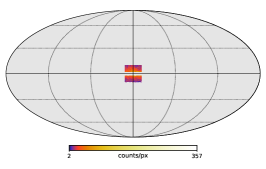
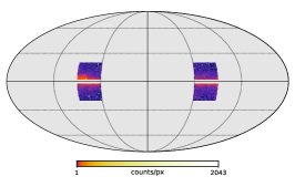
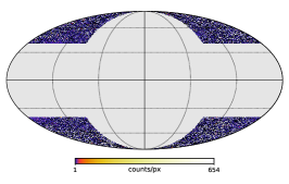
Figure S3: Left panel: Region of interest for the 1pPDF analysis in the Inner Galaxy. Middle panel: Outer Galaxy. Right panel: extragalactic. The Fermi-LAT counts per pixel in the energy bin [2, 5] GeV are reported.

We restrict the analysis of Fermi-LAT data to events in the quartile with the best angular reconstruction, i.e. evtype=PSF3. The spatial binning of photon events is performed using the HEALPix equal-area pixelation scheme Gorski et al. (2005) with resoluton parameter $\kappa=7$ Gorski et al. (2005) (the total number of pixels covering the entire sky is $N_{\rm pix}=12N^{2}_{\rm side}$ and $N_{\rm side}=2^{\kappa}$). The analysis is restricted to the $2-5$ GeV energy bin. Previous analyses of the IG using photon-count statistics typically started from 2 GeV to avoid significant PSF smoothing and Galactic diffuse emission systematics at lower energies, while going up to $20$ GeV Lee et al. (2016); Buschmann et al. (2020). We choose to cut at $5$ GeV instead of $20$ GeV as the photon statistics is largely dominated by lower energies, and to easily compare to our previous results at high Galactic latitudes Zechlin et al. (2016a, b). Also, performing the 1pPDF analysis in smaller energy bins might allow to further investigate the nature of IPS, which is left to future work.

A benchmark upper flux cut of $10^{-8}$ ph cm^-2 s^-1 is applied. We do not mask resolved sources, but we model them together with fainter PS to reduce possible systematics connected to the source masking or to additional Poissonian templates. A lower flux cut is only effectively applied within the hybrid method, see next section.

To dissect the source-count distribution of PS in the IG we restrict to specific ROI. The fiducial IG ROI is defined by a $20^{\circ}\times 20^{\circ}$ square around the GC. As discussed in Buschmann et al. (2020), the choice of the ROI can influence the results of photon-count statistical analysis, and needs to be chosen carefully. We found the $20^{\circ}\times 20^{\circ}$ square optimal to contain enough statistics to constrain the IPS parameters, and not too large, to avoid possible over-subtraction of the Galactic diffuse emission Buschmann et al. (2020). Nevertheless, we tested that our main conclusions are unchanged when going to $30^{\circ}\times 30^{\circ}$. Although we cannot test directly in the fit the preference for different PS spatial distributions, we can nevertheless verify if these PS are truly isotropic over the ten-degree scale of the IG ROI, and if they are mainly Galactic or extragalactic. To this end, the IG ROI is partitioned in radial and longitudinal slices to build the profiles shown in Fig. 2. For the sake of definiteness, the corresponding portions of the IG are illustrated in Fig. S4.

Furthermore, two additional ROIs are used to investigate the nature of the IPS found in the IG ROI: The outer Galaxy (OG, $|b|<20^{\circ}$, $60^{\circ}<|l|<90^{\circ}$) and the extragalactic ((EG, $|b|>40^{\circ}$, $|l|>90^{\circ}$) ROIs. The first is meant to represent Galactic IPS, but away from the GC, while the second to provide the truly extragalactic population of IPS. We define the OG such that, from the skyFACT runs, we do not have any longer evidence for a GCE emission. Since there is no evidence for the GCE, the diffuse models obtained with and without this additional component are consistent. For the IG and OG ROIs we also cut the innermost region along the Galactic plane. We test different cuts $|b|>0.5^{\circ},2^{\circ},4^{\circ}$, finding consistent results. We stress that a latitude cut of $2^{\circ}$ was used in past analyses Lee et al. (2016); Buschmann et al. (2020); Leane and Slatyer (2020a), while we demonstrate the consistency of our results down to $0.5^{\circ}$ for the first time.

An illustration of these three ROIs is provided in Fig. S3. For each ROI, the counts per pixel of Fermi-LAT data in the energy bin $2-5$ GeV and for the analysis cuts described in this section are reported.

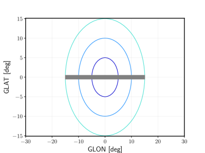
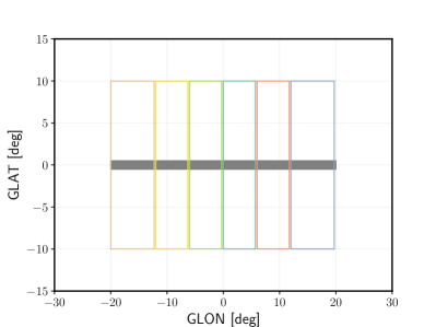
Figure S4: Radial and longitude slices. The Inner Galaxy division in radial (longitude) slices in the left (right) panel used for computing the source number density depicted in Fig. 2, with consistent color coding.

S2.3 Model parameters, priors, fitting procedure

We recall that the 1pPDF fits to Fermi-LAT data are performed with the following components: Isotropic diffuse emission template, diffuse emission template (optimized or not through skyFACT fit), IPS population with source-count distribution per unit flux $dN/dS$ and, if included, a diffuse template describing the GCE, following a Galactic bulge or DM morphology. The IPS population is described by a unique multiple broken power law (MBPL, see Eq. (1)) with two or three free breaks, while the Poissonian components have one free normalization each. The normalization constant in Eq. (1) is fixed to $S_{0}=5\cdot 10^{-9}$ ph cm^-2 s^-1 . The results presented in the main text have been obtained using a Galactic diffusion emission template optimized by skyFACT, to reduce background systematics. Results using alternative diffuse emission templates are discussed in the following. Both the diffuse emission templates and the GCE templates used as inputs for the 1pPDF fits are the optimized outputs of skyFACT, and enter the 1pPDF fits with an additional free normalization, $A_{\rm gal}$ and $A_{\rm B/NFW126}$, respectively. The pixel-dependent likelihood function $\mathcal{L}({\bf\Theta})$ is defined following the L2 method in Zechlin et al. (2016a). In this way, the spatial morphology of the skyFACT diffuse templates is taken into account in the 1pPDF fits. In fact, while below the sensitivity of the 1pPDF method the PS in the ultra-faint regime are in principle degenerate with a diffuse emission, our pixel dependent likelihood is sensitive to the morphology of the diffuse spatial templates. The full list of free parameters $\Theta$, along with their prior intervals are summarized in Tab. SIII.

Table SIII: Prior types and ranges for the 1pPDF analysis of the IG. The first two parameters are in common with all the setups, while the third is present only in the 1pPDF-B, 1pPDF-NFW126 analyses. The second block refers to the parameters for the IPS when using the MBPL fit approach, while the last one to the Hybrid approach, where the MBPL was extended with a node. The normalizations $A_{S},\,A_{\rm nd1}$ are given in units of s cm²sr^-1. The break positions $S_{\rm bn,snd1}$ are in units of ph cm^-2 s^-1 . The $F_{\rm iso}$ is given in units of cm²s^-1sr^-1. All other parameters are dimensionless.

Method	Parameter	Prior	Range $N_{b}=2$ (=3)
	$A_{\rm gal}$	log-flat	[0.1,10]
	$F_{\rm iso}$	log-flat	[$10^{-11}$, $10^{-8}$]
	$A_{\rm B/NFW126}$	log-flat	[$10^{-2}$, $10^{2}$]
MBPL	$A_{S}$	log-flat	[$10^{8}$, $5\cdot 10^{11}$]
	$S_{\rm b1}$	log-flat	[$5\cdot 10^{-9}$, $10^{-8}$]
	$S_{\rm b2}$	log-flat	[$10^{-13}$ ($5\cdot 10^{-10}$), $5\cdot 10^{-9}$]
	$S_{\rm b3}$	log-flat	[…($10^{-13}$), …($5\cdot 10^{-10}$)]
	$n_{\rm 1}$	flat	[-1, 3]
	$n_{\rm 2}$	flat	[-1, 3.5]
	$n_{\rm 3}$	flat	[-2 (1), 2 (3)]
	$n_{\rm 4}$	flat	[…(-2),…(2)]
Hybrid	$A_{S}$	log-flat	[$10^{8}$, $5\cdot 10^{11}$]
	$S_{\rm b1}$	log-flat	[$10^{-9}$, $10^{-8}$]
	$S_{\rm b2}$	log-flat	[$10^{-11}$($2\cdot 10^{-10}$), $10^{-9}$]
	$S_{\rm b3}$	log-flat	[…($10^{-11}$), …($2\cdot 10^{-10}$)]
	$n_{\rm 1}$	flat	[2.5 ,4.3]
	$n_{\rm 2}$	flat	[1.3,2.3]
	$n_{\rm 3}$	flat	[1.3,3]
	$n_{\rm 4}$	flat	[…(1.3),…(3)]
	$A_{\rm nd1}$	log-flat	[$10^{14}$, $10^{17}$]
	$S_{\rm nd1}$	fixed	$5\cdot 10^{-12}$($3\cdot 10^{-12}$)
	$n_{\rm f}$	fixed	-10

To sample the posterior distribution $P({\bf\Theta})=\mathcal{L}({\bf\Theta})\pi({\bf\Theta})/\mathcal{Z}$ (where $\pi({\bf\Theta})$ is the prior and $\mathcal{Z}$ is the Bayesian evidence) the MultiNest framework Feroz et al. (2009) was used in its standard configuration, setting 1000 live points with a tolerance criterion of 0.2. One-dimensional profile likelihood functions Rolke et al. (2005) for each parameter are built from the final posterior sample in order to get prior-independent frequentist parameter estimates. If not differently stated, best-fit parameter estimates refer to the obtained maximum likelihood parameter values. Consistent results are found for the Bayesian parameter estimation. The nested sampling global log-evidence $\ln(\mathcal{Z})$ is used to build Bayes factors for model comparison, see main text.

Different fitting techniques have been introduced within the 1pPDF framework Zechlin et al. (2016a). We here use the MBPL approach as benchmark, where the parameters of the MBPL in Eq. (1) are sampled directly. To check for possible systematics introduced in the ultra-faint regime, we also perform our analysis using the Hybrid approach (see Zechlin et al. (2016a) for details). This is characterized by fixing a grid number of nodes (i.e. fixed flux positions) for the $dN/dS$ fit, around the sensitivity threshold of the analysis. The Hybrid approach was introduced to address possible underestimation or bias in the reconstructed source-count distribution fit and its uncertainty bands at the lower end of the faint-source regime, as demonstrated using Montecarlo simulations in Zechlin et al. (2016a). This has been shown to alleviate possible bias when measuring the $dN/dS$ in the ultra-faint regime, which can cause a loss of sensitivity of the method.

S3 Diffuse emission template systematics

One of the main novelties of this work is the fact to employ consistently diffuse emission models optimized using skyFACT within the 1pPDF. We here apply the 1pPDF to the IG using other widely used diffuse emission templates: The official spatial and spectral template released by the Fermi-LAT Collaboration for Pass 8 data (Official P8) (gll_iem_v06.fits, see Ref. Acero et al. (2016)), and the models labeled A (modA) and B (modB), optimized for the study of the IGRB in Ackermann et al. (2015). We note that within modA and modB the Fermi bubbles are not modeled. The results for the $dN/dS$ of the IG are illustrated in the left (right) panel of Fig. S5 when cutting the innermost $2^{\circ}$ ($4^{\circ}$).

By using standard diffuse models (modA, modB and Official P8), we reconstruct spurious sources at $\sim 4\times 10^{-10}$ ph cm^-2 s^-1, well above the sensitivity of the 1pPDF. Such a peak of the IPS $dN/dS$ disappears instead if we use diffuse emission templates as optimized with skyFACT. Large scale residuals are indeed reduced when allowing the spatial diffuse templates to be remodulated in the fit. Even in the absence of an additional GCE template, the skyFACT fit remodulates the diffuse components such to partially absorbs GCE photons, therefore reducing residuals and improving the fit with respect to standard diffuse models. Also, in this ROI, all the diffuse models, except the skyFACT one, do not properly reproduce the 4FGL catalog bright sources. We notice that the spurious IPS peak of the $dN/dS$ corresponds to a peak of flagged 4FGL sources, further corroborating the conclusion that it is indeed a spurious reconstruction effect. We stress that any comparison with 4FGL cataloged sources is purely illustrative, and serves for cross-checking our results at high fluxes.

We therefore confirm previous findings Buschmann et al. (2020) that large residuals due to mis-modelling of diffuse emission induce a bias in the reconstruction of PS in the inner Galaxy.

We also identify spatially critical regions within the IG where this mis-modeling effect is more pronounced, notably the Northern hemisphere (both West and East quadrants). This might be connected to the North/South asymmetry found within the NPTF analysis of the GCE discussed in Leane and Slatyer (2020a). As shown in Fig. S6 the spurious IPS peak of the $dN/dS$ reconstructed with the 1pPDF using the Official P8 template is found to be strongly pronounced in the North IG ROI in the same flux region as found in Fig. S5, while it is not present in the analysis of the South IG ROI. When using the diffuse emission templates as obtained with skyFACT, we find instead a smoother $dN/dS$ which is compatible within $1\sigma$ uncertainty with the 4FGL unflagged sources. Moreover, the 1pPDF results for the $dN/dS$ using the Official P8 and the skyFACT diffuse templates in the South IG ROI are compatible within the obtained $1\sigma$ bands.

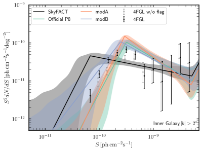
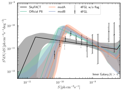
Figure S5: Diffuse emission systematics. Source count distribution in the IG obtained from the 1pPDF analysis cutting the inner $2^{\circ}$ (left panel) and $4^{\circ}$(right panel). The black line is obtained from the 1pPDF when using the model for the Galactic diffuse emission obtained from skyFACT (without any component modeling the GCE, sF-noGCE). The colored lines are instead obtained from the 1pPDF using the official Fermi-LAT model for Pass 8 (cyan line), or modA and modB (orange and indaco lines). The black (gray) points represent the count distribution of 4FGL sources (without any analysis flag, intended as a cautionary index for the reality of a source or the magnitude of its systematic uncertainties Abdollahi et al. (2020)).

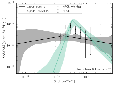
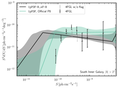
Figure S6: North and South Inner Galaxy. Left (right) panel: Source-count distribution of the North (South) region of the IG obtained from the 1pPDF  analysis. Results are here reported using the Official P8 and the sF-B models for the diffuse emission. Points as in Fig. S5.

S4 $dN/dS$ modeling systematics

The stability of the $dN/dS$ results in the IG from the combined 1pPDF-skyFACT analysis of Fermi-LAT data was tested against a number of systematics.

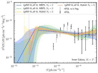
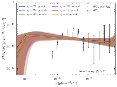
Figure S7: Systematic for $dN/dS$ reconstruction in the IG. Source count distribution of the IG obtained from the 1pPDF analysis cutting the inner 2^∘. Left panel: Effect of the number of free breaks $N_{\rm b}$ (dashed lines) and of the Hybrid fit approach with different number of breaks and varying the node position. The dotted line illustrates the position of $S_{\rm nd1}$ for the corresponding Hybrid fit. Right panel: Effect of the smoothing scales $\eta_{\rm g,b}$ used to obtain the skyFACT diffuse emission. Points as in Fig. S5.

The $dN/dS$ in the IG and OG is well described by a MBPL with two free breaks. We verified that an additional free break is not preferred by data, and that the MBPL obtained with three free breaks (see prior intervals in Table SIII) is compatible, within the uncertainties, with the case of two free breaks. This is illustrated in the left panel of Fig. S7.

Fluxes from bright sources with $S>10^{-8}$ ph cm^-2 s^-1 are not considered in the 1pPDF analysis. We verified that shifting the upper flux cut down to $S>10^{-9}$ ph cm^-2 s^-1 does not change our main results. The only difference we observe is a change in the position of the first flux break, driven by few, bright sources, always compatible with 4FGL points and uncertainties within $1-2\sigma$ C.L. As for the low-flux regime, in our benchmark 1pPDF setup we do not include any lower flux cut. To test for possible effects connected to the faint end of the source-count distribution, we repeated the main analysis using the hybrid approach introduced in Zechlin et al. (2016a). We set a fixed node at $S_{\rm nd1}$, with the index of the power-law component below the last node, $n_{f}=-10$, thus effectively suppressing possible contributions in the ultra-faint regime below the fixed node. Note that a fixed node $S_{\rm nb0}$ at the lower limit of the prior for the last free break is technically imposed, since the first free node $S_{\rm nb1}$ is continuously connected to the MBPL component with a power law at higher fluxes. We tested different values for the position of $S_{\rm nd1}$ in the faint source regime, together with a MBPL with two or three free breaks. Results are summarized in the left panel of Fig. S7. To the extent we have tested, a node in the faint source regime at $3-5\cdot 10^{-12}$ ph cm^-2 s^-1 does not affect the reconstructed $dN/dS$ of the IG, which is well compatible, within $1\sigma$ uncertainty bands, with the benchmark results discussed in Fig. 1. In particular, the $dN/dS$ is well compatible in the flux interval $10^{-11}-10^{-9}$ ph cm^-2 s^-1 , where the radial and longitude profiles are computed.

We also tested the effect on the 1pPDF results of changing the smoothing scale $\eta$ of the Galactic diffuse components in the skyFACT fit. The benchmark values used for the results illustrated so far are $\eta_{\rm g}=25$ and $\eta_{\rm b}=4$ for the gas and the Fermi bubbles components, respectively. Variations for $\eta_{\rm b}=25$ and different values for $\eta_{\rm g}=400,100,11,4$ are tested to assess possible systematic connected to this choice. In fact, a higher value of $\eta$ corresponds to a higher smoothing in the skyFACT template used for 1pPDF analysis. A different smoothing scale in the skyFACT diffuse template could affect the reconstructed $dN/dS$ in the 1pPDF, as this could leave residuals at small angular scales that could be wrongly attributed to PS by the 1pPDF. In Fig. S7 the corresponding results for the $dN/dS$ are reported, compared to the benchmark results also shown in Fig. 1. This test is performed using the sF-B diffuse emission within the 1pPDF-B fit. The best fit and $1\sigma$ band of the reconstructed source-count distribution are consistent for all the explored variations in $\eta_{\rm b,g}$. The same is true for the best-fit parameters of the IPS. As for the other 1pPDF parameters, variations of $\eta_{\rm b}$ do not affect significantly the best fit of $A_{B}$ and the $\ln(\mathcal{Z})$. We instead observe a slight decrease (increase) of $\ln(\mathcal{Z})$ for decreasing (increasing) $\eta_{\rm g}$. This is expected, as for smaller $\eta_{\rm g}$ in the skyFACT fit the Galactic diffuse emission gas template can more easily account for small variations between adjacent pixels, decreasing the overall residuals.

Finally, we note that, when analyzing the inner Galaxy divided in rings as shown in Fig.S4, the best-fit normalization for $A_{B}$ decreases slightly going towards the innermost ring. However, the uncertainties get larger, making the bulge template normalization $A_{B}$ in the rings still compatible with the numbers shown in Table I within $1\sigma$ uncertainties.

S5 Outer Galaxy and extragalactic $dN/dS$ results

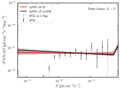
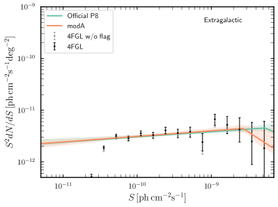
Figure S8: Outer Galaxy and extragalactic $dN/dS$. Source count distribution of the outer Galaxy (left panel) and of the extragalactic ROI (right panel) obtained from the 1pPDF analysis. Outer Galaxy: Results for the $dN/dS$ are reported for two cases: (i) using the skyFACT Galactic diffuse emission model without any component modeling the GCE (black line), and for the benchmark sF-B model, where an additional component modeling the bulge is added. Extragalactic: Results are here reported using the Official P8 model and modA. Points as in Fig. S5.

We finally report extended results on the OG and EG ROI, which are illustrated in Fig. S8. We note that in these ROI there are no 4FGL flagged sources, and the $dN/dS$ is well described by a single power law from $S\sim 3\cdot 10^{-9}$ ph cm^-2 s^-1 down to $S\sim 10^{-11}$ ph cm^-2s^-1. The IPS in the OG and EG are well consistent with 4FGL source counts for bright sources. In both cases, we obtain compatible results among different Galactic diffuse emission models, both for skyFACT (left panel) or for the Official P8 and modA (right panel). Results for the [2, 5] GeV IPS in the EG are also well compatible with previous studies Zechlin et al. (2016b, 2018).

References

- Abazajian and Kaplinghat (2012) K. N. Abazajian and M. Kaplinghat, Phys. Rev. D86, 083511 (2012), arXiv:1207.6047 [astro-ph.HE] .
- Gordon and Macias (2013) C. Gordon and O. Macias, Phys. Rev. D88, 083521 (2013), [Erratum: Phys. Rev.D89,no.4,049901(2014)], arXiv:1306.5725 [astro-ph.HE] .
- Calore et al. (2015a) F. Calore, I. Cholis, and C. Weniger, JCAP 03, 038 (2015a), arXiv:1409.0042 [astro-ph.CO] .
- Daylan et al. (2016) T. Daylan, D. P. Finkbeiner, D. Hooper, T. Linden, S. K. N. Portillo, N. L. Rodd, and T. R. Slatyer, Phys. Dark Univ. 12, 1 (2016), arXiv:1402.6703 [astro-ph.HE] .
- Ajello et al. (2016) M. Ajello et al. (Fermi-LAT), Astrophys. J. 819, 44 (2016), arXiv:1511.02938 [astro-ph.HE] .
- Navarro et al. (1997) J. F. Navarro, C. S. Frenk, and S. D. M. White, Astrophys. J. 490, 493 (1997), arXiv:astro-ph/9611107 .
- Calore et al. (2015b) F. Calore, I. Cholis, C. McCabe, and C. Weniger, Phys. Rev. D91, 063003 (2015b), arXiv:1411.4647 [hep-ph] .
- Agrawal et al. (2015) P. Agrawal, B. Batell, P. J. Fox, and R. Harnik, JCAP 05, 011 (2015), arXiv:1411.2592 [hep-ph] .
- Murgia (2020) S. Murgia, Ann. Rev. Nucl. Part. Sci. 70, 455 (2020).
- Di Mauro (2021) M. Di Mauro, (2021), arXiv:2101.04694 [astro-ph.HE] .
- Abazajian (2011) K. N. Abazajian, Journal of Cosmology and Astroparticle Physics 1103, 010 (2011), arXiv:1011.4275 [astro-ph.HE] .
- Bartels et al. (2018) R. Bartels, E. Storm, C. Weniger, and F. Calore, Nature Astronomy 2, 819 (2018), arXiv:1711.04778 [astro-ph.HE] .
- Macias et al. (2018) O. Macias, C. Gordon, R. M. Crocker, B. Coleman, D. Paterson, S. Horiuchi, and M. Pohl, Nature Astronomy 2, 387 (2018), arXiv:1611.06644 [astro-ph.HE] .
- Macias et al. (2019) O. Macias, S. Horiuchi, M. Kaplinghat, C. Gordon, R. M. Crocker, and D. M. Nataf, JCAP 09, 042 (2019), arXiv:1901.03822 [astro-ph.HE] .
- Bartels et al. (2016) R. Bartels, S. Krishnamurthy, and C. Weniger, Phys. Rev. Lett. 116, 051102 (2016), arXiv:1506.05104 [astro-ph.HE] .
- Lee et al. (2016) S. K. Lee, M. Lisanti, B. R. Safdi, T. R. Slatyer, and W. Xue, Phys. Rev. Lett. 116, 051103 (2016), arXiv:1506.05124 [astro-ph.HE] .
- Leane and Slatyer (2019) R. K. Leane and T. R. Slatyer, Phys. Rev. Lett. 123, 241101 (2019), arXiv:1904.08430 [astro-ph.HE] .
- Leane and Slatyer (2020a) R. K. Leane and T. R. Slatyer, Phys. Rev. Lett. 125, 121105 (2020a), arXiv:2002.12370 [astro-ph.HE] .
- Chang et al. (2020) L. J. Chang, S. Mishra-Sharma, M. Lisanti, M. Buschmann, N. L. Rodd, and B. R. Safdi, Phys. Rev. D 101, 023014 (2020), arXiv:1908.10874 [astro-ph.CO] .
- Buschmann et al. (2020) M. Buschmann, N. L. Rodd, B. R. Safdi, L. J. Chang, S. Mishra-Sharma, M. Lisanti, and O. Macias, Phys. Rev. D 102, 023023 (2020), arXiv:2002.12373 [astro-ph.HE] .
- Zhong et al. (2020) Y.-M. Zhong, S. D. McDermott, I. Cholis, and P. J. Fox, Phys. Rev. Lett. 124, 231103 (2020), arXiv:1911.12369 [astro-ph.HE] .
- Leane and Slatyer (2020b) R. K. Leane and T. R. Slatyer, Phys. Rev. D 102, 063019 (2020b), arXiv:2002.12371 [astro-ph.HE] .
- Caron et al. (2018) S. Caron, G. A. Gómez-Vargas, L. Hendriks, and R. Ruiz de Austri, JCAP 05, 058 (2018), arXiv:1708.06706 [astro-ph.HE] .
- List et al. (2020) F. List, N. L. Rodd, G. F. Lewis, and I. Bhat, Phys. Rev. Lett. 125, 241102 (2020), arXiv:2006.12504 [astro-ph.HE] .
- Calore et al. (2016) F. Calore, M. Di Mauro, F. Donato, J. W. T. Hessels, and C. Weniger, ApJ 827, 143 (2016), arXiv:1512.06825 [astro-ph.HE] .
- Calore et al. (2019) F. Calore, T. Regimbau, and P. D. Serpico, PRL 122, 081103 (2019), arXiv:1812.05094 [astro-ph.HE] .
- Berteaud et al. (2020) J. Berteaud, F. Calore, M. Clavel, P. D. Serpico, G. Dubus, and P.-O. Petrucci, (2020), arXiv:2012.03580 [astro-ph.HE] .
- Storm et al. (2017) E. Storm, C. Weniger, and F. Calore, JCAP 08, 022 (2017), arXiv:1705.04065 [astro-ph.HE] .
- Malyshev and Hogg (2011) D. Malyshev and D. W. Hogg, ApJ 738, 181 (2011), arXiv:1104.0010 [astro-ph.CO] .
- Zechlin et al. (2016a) H.-S. Zechlin, A. Cuoco, F. Donato, N. Fornengo, and A. Vittino, Astrophys. J. Suppl. 225, 18 (2016a), arXiv:1512.07190 [astro-ph.HE] .
- Zechlin et al. (2016b) H.-S. Zechlin, A. Cuoco, F. Donato, N. Fornengo, and M. Regis, Astrophys. J. Lett. 826, L31 (2016b), arXiv:1605.04256 [astro-ph.HE] .
- Manconi et al. (2020) S. Manconi, M. Korsmeier, F. Donato, N. Fornengo, M. Regis, and H. Zechlin, Phys. Rev. D 101, 103026 (2020), arXiv:1912.01622 [astro-ph.HE] .
- Zechlin et al. (2018) H.-S. Zechlin, S. Manconi, and F. Donato, Phys. Rev. D 98, 083022 (2018), arXiv:1710.01506 [astro-ph.HE] .
-
(34)
Publicly available at
https://heasarc.gsfc.nasa.gov/
FTP/fermi/data/lat/weekly/photon/. More details are found at https://fermi.gsfc.nasa.gov/ssc/data/analysis/documentation/Cicerone/Cicerone_Data/LAT_DP.html. - (35) This ROI still allows to discriminate the GCE morphology without suffering from systematics induced by selecting too narrow ROIs Macias et al. (2019).
- Abdollahi et al. (2020) S. Abdollahi et al. (Fermi-LAT), Astrophys. J. Suppl. 247, 33 (2020), arXiv:1902.10045 [astro-ph.HE] .
- (37) See Supplemental Material at [URL will be inserted by publisher]. Sec. I for details on the SkyFACT analysis, Sec. II for details on the 1pPDF analysis, Sec. III-IV for systematic checks on the diffuse emission template and dN/dS modeling within the 1pPDF, and Sec. V for the dN/dS of the outer and extragalactic regions.
- (38) As currently implemented, the 1pPDF method does not allow to test spatially-dependent .
- Ackermann et al. (2015) M. Ackermann et al., ApJ 799, 86 (2015), arXiv:1410.3696 [astro-ph.HE] .
- Maccione et al. (2011) L. Maccione, C. Evoli, D. Gaggero, and D. Grasso, “DRAGON: Galactic Cosmic Ray Diffusion Code,” (2011), ascl:1106.011 .
- Ackermann and others (2012) M. Ackermann and others, ApJ 750, 3 (2012), arXiv:1202.4039 [astro-ph.HE] .
- Ackermann et al. (2014) M. Ackermann et al. (Fermi-LAT), Astrophys. J. 793, 64 (2014), arXiv:1407.7905 [astro-ph.HE] .
- Mishra-Sharma et al. (2017) S. Mishra-Sharma, N. L. Rodd, and B. R. Safdi, Astron. J. 153, 253 (2017), arXiv:1612.03173 [astro-ph.HE] .
- Gorski et al. (2005) K. M. Gorski, E. Hivon, A. J. Banday, B. D. Wandelt, F. K. Hansen, M. Reinecke, and M. Bartelmann, ApJ 622, 759 (2005), astro-ph/0409513 .
- Feroz et al. (2009) F. Feroz, M. P. Hobson, and M. Bridges, MNRAS 398, 1601 (2009), arXiv:0809.3437 .
- Rolke et al. (2005) W. A. Rolke, A. M. López, and J. Conrad, Nuclear Instruments and Methods in Physics Research A 551, 493 (2005), physics/0403059 .
- Acero et al. (2016) F. Acero et al., ApJS 223, 26 (2016), arXiv:1602.07246 [astro-ph.HE] .