Finite-momentum energy dynamics in a Kitaev magnet

Abstract

We study the energy-density dynamics at finite momentum of the two-dimensional Kitaev spin-model on the honeycomb lattice. Due to fractionalization of magnetic moments, the energy relaxation occurs through mobile Majorana matter, coupled to a static $\mathbb{Z}_{2}$ gauge field. At finite temperatures, the $\mathbb{Z}_{2}$ flux excitations act as an emergent disorder, which strongly affects the energy dynamics. We show that sufficiently far above the flux proliferation temperature, but not yet in the classical regime, gauge disorder modifies the coherent low-temperature energy-density dynamics into a form which is almost diffusive, with hydrodynamic momentum scaling of a diffusion-kernel, which however remains retarded, primarily due to the presence of two distinct relaxation channels of particle-hole and particle-particle nature. Relations to thermal conductivity are clarified. Our analysis is based on complementary calculations in the low-temperature homogeneous gauge and a mean-field treatment of thermal gauge fluctuations, valid at intermediate and high temperatures.

I Introduction

Ever since the discovery of large magnetic heat transport in quasi one-dimensional (1D) local-moment systems Sologubenko2000a ; Kawamata2008 ; Hlubek2010 ; Sologubenko2000b ; Hess2001 , the dynamics of energy in quantum magnets Zotos1997 ; Heidrich-Meisner2003 ; Heidrich-Meisner2004 , has been a topic of great interest Hess2007 ; FHM2007 ; Hess2019 ; Bertini2020 . Unfortunately, rigorous theoretical progress has essentially remained confined to 1D Bertini2020 . Above 1D, understanding energy dynamics in quantum magnets remains an open issue at large. If magnetic long range order (LRO) is present and magnons form a reliable quasi particle basis, various insights have been gained for antiferromagnets and cuprates Dixon1980 ; Hess2003 ; Bayrakci2013 ; Chernyshev2016 . If LRO is absent, and in particular in quantum spin liquids (QSL) Balents2010 ; Balents2016 , energy transport has recently come into focus as a probe of potentially exotic elementary excitations. In fact, experiments in several quantum disordered, frustrated spin systems in $D\geq 2$ suggest unconventional magnetic energy dynamics. For bulk transport, this pertains, e.g., to quasi 2D triangular organic salts Yamashita2010 ; Bourgeois2019 ; Ni2019 , or to 3D quantum spin ice materials Kolland2012 ; Toews2012 ; Tokiwa2018 . For boundary transport, i.e., the magnetic thermal Hall effect, recent examples include Kagomé magnets Hirschberger2015a ; Watanabe2016 ; Yamashita2019 and spin ice Hirschberger2015b . A microscopic description of such observations is mostly lacking.

In this context, Kitaev’s compass exchange Hamiltonian on the honeycomb lattice is of particular interest, as it is one of the few models, in which a $\mathbb{Z}_{2}$ QSL can exactly be shown to exist Kitaev2006 . The spin degrees of freedom of this model fractionalize in terms of mobile Majorana fermions coupled to a static $\mathbb{Z}_{2}$ gauge field Kitaev2006 ; Feng2007 ; Chen2008 ; Nussinov2009 ; Mandal2012 . From a material’s perspective, $\alpha$-RuCl₃ Plumb2014 may be a promising candidate for this model Trebst2017 . Free mobile Majorana fermions have been invoked to interpret ubiquitous unconventional continua in spectroscopies on various Kitaev materials, like inelastic neutron Banerjee2016 ; Banerjee2016a ; Banerjee2018 and Raman scattering Knolle2014 ; Wulferding2020 , as well as local resonance probes Baek2017 ; Zheng2017 .

Clearly, Majorana fermions should also play a role in the energy dynamics in putative Kitaev materials. However, bulk thermal conductivity, i.e., $\kappa_{xx}$ in $\alpha$-RuCl₃ Hirobe2017 ; Leahy2017 ; Hentrich2018 ; Yu2018 , seems to be governed primarily by phonons, with phonon-Majorana scattering as a potential dissipation mechanism Hentrich2018 ; Yu2018 ; Metavitsiadis2020a . Yet, Majorana fermions may have been observed in the transverse energy conductivity $\kappa_{xy}$ in magnetic fields, i.e., in the thermal Hall effect, and its alleged quantization Kasahara2018 ; Yokoi2020 . In view of this, energy transport in Kitaev spin liquids has been the subject of several theoretical studies Metavitsiadis2017a ; Nasu2017 ; Metavitsiadis2017 ; Pidatella2019 ; Metavitsiadis2019 ; Metavitsiadis2020b . Previous investigations however, have focused on energy-current correlation functions and at zero momentum only.

In this work, we take a different perspective and consider the energy-density correlation function directly and at finite momentum. In particular we will be interested in the role, which the emergent disorder introduced by thermally excited $\mathbb{Z}_{2}$ gauge field plays in the long wave-length regime. Therefore, we map out the energy diffusion kernel of the Kitaev model and its momentum and energy dependence, ranging from low, up to intermediate temperatures and we contrast this with expectation for simple diffusion in random systems. The paper is organized as follows. In Section II, we briefly recapitulate the Kitaev model. In Section III, details of our calculations are provided, for the homogeneous and the random gauge state in Subsections III.1 and III.2, respectively, and the extraction of the diffusion kernel is described in Subsection III.3. We discuss our results in Section IV and summarize in Section V. An Appendix, App. A, on generalized Einstein relations is included.

II Model

We consider the Kitaev spin-model on the two dimensional honeycomb lattice

$$H=\sum_{{\bf l},\alpha}J_{\alpha}S_{{\bf l}}^{\alpha}S_{{\bf l}+{\bf r}_{\alpha}}^{\alpha}\,,$$ (1)

where ${\bf l}=n_{1}{\bf R}_{1}+n_{2}{\bf R}_{2}$ runs over the sites of the triangular lattice with ${\bf R}_{1[2]}=(1,0),\,[(\frac{1}{2},\frac{\sqrt{3}}{2})]$ for lattice constant $a{\equiv}1$, and ${\bf r}_{\alpha=x,y,z}=(\frac{1}{2},\frac{1}{2\sqrt{3}}),$ $(-\frac{1}{2},\frac{1}{2\sqrt{3}})$, $(0,-\frac{1}{\sqrt{3}})$ refer to the basis sites $\alpha=x,y,z$, tricoordinated to each lattice site of the honeycomb lattice. As extensive literature, rooted in Ref. Kitaev2006 , has clarified, Eq. (1) can be mapped onto a bilinear form of Majorana fermions in the presence of a static $\mathbb{Z}_{2}$ gauge $\eta_{{\bf l}}=\pm 1$, residing on, e.g., the $\alpha=z$ bonds

$$H=-\frac{i}{2}\sum_{{\bf l},\alpha}J_{\alpha}\eta_{{\bf l},\alpha}\,a_{{\bf l}}c_{{\bf l}+{\bf r}_{\alpha}}\,.$$ (2)

Here we introduce $\eta_{{\bf l},\alpha}$ to unify the notation, with $\eta_{{\bf l},x(y)}=1$ and $\eta_{{\bf l},z}=\eta_{{\bf l}}$. There are two types of Majorana particles, corresponding to the two basis sites. We chose to normalize them as $\{a_{{\bf l}},a_{{\bf l}^{\prime}}\}=\delta_{{\bf l},{\bf l}^{\prime}}$, $\{c_{{\bf m}},c_{{\bf m}^{\prime}}\}=\delta_{{\bf m},{\bf m}^{\prime}}$, and $\{a_{{\bf l}},c_{{\bf m}}\}=0$. For each gauge sector $\{\eta_{{\bf l}}\}$, Eq. (2) represents a spin liquid.

For the purpose of this work a local energy density $h_{{\bf c}}$ on some repeating “unit” cluster ${\bf c}$ has to be chosen. Obviously $H=\sum_{{\bf c}}h_{{\bf c}}$. As for any local density, the latter does not fix a unique expression for $h_{{\bf c}}$. Different shapes of the real-space clusters ${\bf c}$ supporting $h_{{\bf c}}$ will typically lead to differing high-frequency and short wave-length spectra for its autocorrelation function. However the low-frequency, long-wave-length dynamics is governed by energy conservation and will not depend on a particular choice of $h_{{\bf c}}$ qualitatively Metavitsiadis2020b . For the remainder of this work we therefore set ${\bf c}={\bf l}$, focusing on $h_{{\bf l}}=-(i/2)\sum_{\alpha}J_{\alpha}\eta_{{\bf l},\alpha}\,a_{{\bf l}}c_{{\bf l}+{\bf r}_{\alpha}}$, i.e. the energy density formed by the tricoordinated bonds around each site on the triangular lattice. Its Fourier transform is $h_{{\bf q}}=\sum_{{\bf l}}e^{i{\bf q}\cdot{\bf l}}h_{{\bf l}}$ with $h_{{\bf q}}^{\dagger}=h_{-{\bf q}}$ and $h_{{\bf 0}}=H$

III Energy Susceptibilty

In this section, we present our evaluation of the dynamical energy susceptibility. We focus on two temperature regimes, namely $T\lesssim(\gtrsim)T^{\star}$. Here $T^{\star}$ is the so called flux proliferation temperature. In the vicinity of this temperature the gauge field and therefore fluxes get thermally excited. Previous analysis Nasu2015 ; Metavitsiadis2017 ; Pidatella2019 ; Metavitsiadis2020b has shown, that the temperature range over which a complete proliferation of fluxes occurs is confined to a rather narrow region, less than a decade centered around $T^{\star}\approx 0.012J$ for isotropic exchange, $J_{z,y,x}$=$J$, used in this work, and decrease rapidly with anisotropy Nasu2015 ; Pidatella2019 . Our strategy therefore is to consider a homogeneous ground state gauge, i.e., $\eta_{{\bf l}}=1$ for $T\lesssim T^{\star}$ and a completely random-gauge states for $T\gtrsim T^{\star}$. This approach has proven to work very well on a quantitative level in several studies of the thermal conductivity of Kitaev models Metavitsiadis2017 ; Pidatella2019 ; Metavitsiadis2017a . Note that for $\alpha$-RuCl₃, the case of $T\lesssim T^{\star}$ is more of conceptual, than of practical interest, since it refers to very low temperatures, assuming a generally accepted $|J|\sim 85K$ Banerjee2016 .

III.1 Homogeneous gauge for $T\lesssim T^{\star}$

For $\eta_{{\bf l}}=1$, the Hamiltonian (1) can be diagonalized analytically in terms of complex Dirac fermions. Mapping from the real Majorana fermions to the latter can be achieved in various ways, all of which require some type of linear combination of real fermions in order to form complex ones. Here we do the latter by using Fourier transformed Majorana particles, $a_{{\bf k}}^{\phantom{\dagger}}=\sum_{{\bf l}}e^{-i{\bf k}\cdot{\bf l}}a_{{\bf l}}/\sqrt{N}$ with momentum ${\bf k}$ and analogously for $c_{{\bf k}}^{\phantom{\dagger}}$. The momentum space quantization is chosen explicitly to comprise $\pm{\bf k}$ for each $|{\bf k}|$. Other approaches, involving reshaped lattice structures Feng2007 ; Nussinov2009 , may pose issues regarding the discrete rotational symmetry of the susceptibility.

The fermions introduced in momentum space are complex with $a_{{\bf k}}^{\dagger}=a_{-{\bf k}}^{\phantom{\dagger}}$, i.e., with only half of the momentum states being independent. This encodes, that for each Dirac fermion, there are two Majorana particles. Standard anticommutation relations apply, $\{a_{{\bf k}}^{\phantom{\dagger}},a_{{\bf k}^{\prime}}^{\dagger}\}=\delta_{{\bf k},{\bf k}^{\prime}}$, $\{c_{{\bf k}}^{\phantom{\dagger}},c_{{\bf k}^{\prime}}^{\dagger}\}=\delta_{{\bf k},{\bf k}^{\prime}}$, and $\{a_{{\bf k}}^{(\dagger)}c_{{\bf k}^{\prime}}^{(\dagger)}\}=0$. From this, the diagonal form of $H$ reads

$$H=\sum_{{\bf k},\gamma=1,2}^{\sim}\mathrm{sg}_{\gamma}\,\epsilon_{{\bf k}}\,d_{{\bf k},\gamma}^{\dagger}d_{{\bf k},\gamma}^{\phantom{\dagger}}\,,$$ (3)

where the $\tilde{\sum}$ sums over a reduced “positive” half of momentum space and $\mathrm{sg}_{\gamma}$=1(-1) for $\gamma$=1(2). The quasiparticle energy is $\epsilon_{{\bf k}}=J[3+2\cos(k_{x})+4\cos(k_{x}/2)\cos(\sqrt{3}k_{y}/2)]^{1/2}/2$. In terms of reciprocal lattice coordinates $x,y\in[0,2\pi]$, this reads $\epsilon_{{\bf k}}=J[3+2\cos(x)+2\cos(y)+2\cos(x-y)]^{1/2}/2$ with ${\bf k}=x\,{\bf G}_{1}+y\,{\bf G}_{2}$, where ${\bf G}_{1[2]}=(1,-\frac{1}{\sqrt{3}}),\,[(0,\frac{2}{\sqrt{3}})]$. The quasiparticles are given by

$$\left[\begin{array}[]{c}c_{{\bf k}}\\ a_{{\bf k}}\end{array}\right] =\left[\begin{array}[]{cc}u_{11}({\bf k})&u_{12}({\bf k})\\ u_{21}({\bf k})&u_{22}({\bf k})\end{array}\right]\left[\begin{array}[]{c}d_{1{\bf k}}\\ d_{2{\bf k}}\end{array}\right]\,,$$ (10)

$$u_{11}({\bf k}) =-u_{12}({\bf k})=\frac{i\sum_{\alpha}e^{-i{\bf k}\cdot{\bf r}_{\alpha}}}{2^{3/2}\epsilon_{{\bf k}}}\,,$$

$$u_{21}({\bf k}) =u_{22}({\bf k})=\frac{1}{\sqrt{2}}\,.$$

From the sign change of the quasiparticle energy between bands $\gamma$=1,2 in Eq. (3) it is clear that the relations $a_{{\bf k}}^{\dagger}=a_{-{\bf k}}^{\phantom{\dagger}}$ and $c_{{\bf k}}^{\dagger}=c_{-{\bf k}}^{\phantom{\dagger}}$ for reversing momenta of the original Majorana fermions has to change into $d_{1(2){\bf k}}^{\dagger}=d_{2(1)-{\bf k}}^{\phantom{\dagger}}$, switching also the bands. Indeed this is also born out of the transformation (10). Inserting the latter into $h_{{\bf q}}$, the energy density in the quasiparticle basis reads

$$h_{{\bf q}}= \frac{1}{2}\tilde{\sum_{{\bf k}}}\left\{\left[\begin{array}[]{cc}d_{1{\bf k}+{\bf q}}^{\dagger}&d_{2{\bf k}+{\bf q}}^{\dagger}\end{array}\right]\right.$$ (12)

$$\times\left.\left[\begin{array}[]{cc}\epsilon_{{\bf k}+{\bf q}}{+}\epsilon_{{\bf k}}&\epsilon_{{\bf k}+{\bf q}}{-}\epsilon_{{\bf k}}\\ \epsilon_{{\bf k}}{-}\epsilon_{{\bf k}+{\bf q}}&{-}\epsilon_{{\bf k}+{\bf q}}{-}\epsilon_{{\bf k}}\end{array}\right]\left[\begin{array}[]{c}d_{1{\bf k}}^{\phantom{\dagger}}\\ d_{2{\bf k}}^{\phantom{\dagger}}\end{array}\right]\right\}\,.$$ (17)

As to be expected, $h_{{\bf q}{=}{\bf 0}}=H$ from (3) and the off-diagonal interband transitions vanish in that limit.

The energy density susceptibility $\chi({\bf q},z)$ is obtained from Fourier transformation of the imaginary time density Green’s function $\chi({\bf q},z)=\int_{0}^{\beta}d\tau\langle T_{\tau}(h_{{\bf q}}(\tau)h_{-{\bf q}})\rangle e^{i\omega_{n}\tau}/T$ by analytic continuation of the Bose Matsubara frequency $i\omega_{n}=i2\pi nT\rightarrow z\in\mathbb{C}$ and eventually $z\rightarrow\omega+i0^{+}$. In order to ease geometrical complexity, we refrain from confining the complex fermions to only a reduced “positive” region of momentum space. This comes at the expense of additional anomalous anticommutators like, e.g., $\{d_{1{\bf k}}^{\phantom{\dagger}},d_{2{\bf k}^{\prime}}^{\phantom{\dagger}}\}=\delta_{-{\bf k},{\bf k}^{\prime}}$ and their corresponding contractions. Simple algebra yields

$$\chi({\bf q},z) =\chi^{\mathrm{ph}}({\bf q},z)+\chi^{\mathrm{pp}}({\bf q},z)$$ (18)

$$\chi^{\mathrm{ph}}({\bf q},z) =\frac{1}{N}\sum_{{\bf k}}(\epsilon_{{\bf k}+{\bf q}}{+}\epsilon_{{\bf k}})^{2}\frac{f_{{\bf k}+{\bf q}}(T){-}f_{{\bf k}}(T)}{z-\epsilon_{{\bf k}+{\bf q}}+\epsilon_{{\bf k}}}$$

$$\chi^{\mathrm{pp}}({\bf q},z) =\frac{1}{2N}\sum_{{\bf k}}(\epsilon_{{\bf k}+{\bf q}}{-}\epsilon_{{\bf k}})^{2}\left\{[f_{{\bf k}+{\bf q}}(T){+}f_{{\bf k}}(T){-}1]\right.$$

$$\phantom{aaa}\times\left.\left(\frac{1}{z-\epsilon_{{\bf k}+{\bf q}}-\epsilon_{{\bf k}}}{-}\frac{1}{z+\epsilon_{{\bf k}+{\bf q}}+\epsilon_{{\bf k}}}\right)\right\}\,,$$

where the superscripts ph(pp) indicate particle-hole (particle-particle) or, synonymous intra(inter)band type of intermediate states of the fermions, $f_{{\bf k}}(T)=1/(e^{\epsilon_{{\bf k}}/T}+1)$ is the Fermi function. This concludes the formal details for $T\lesssim T^{\star}$.

III.2 Random gauge for $T\gtrsim T^{\star}$

In a random gauge configuration, translational invariance of the Majorana system is lost, and we resort to a numerical approach in real space. This has been detailed extensively for 1D Metavitsiadis2017a ; Metavitsiadis2020b and 2D Pidatella2019 ; Metavitsiadis2017 ; Metavitsiadis2020a models and is only briefly reiterated here for completeness sake. First a spinor $A_{\text{ $\sigma$}}^{\dagger}=(a_{1}\dots a_{{\bf l}}\dots a_{N},c_{1}\dots c_{{\bf l}+{\bf r}_{x}}\dots c_{N})$, comprising the Majoranas on the $2N$ sites of the lattice is defined. Using this, the energy density $h_{{\bf q}}$ and the Hamiltonian (2), i.e., $h_{{\bf 0}}$, are rewritten as $h_{{\bf q}}={\bf A}^{\dagger}{\bf g}_{{\bf q}}{\bf A}/2$. Bold faced symbols refer to vectors and matrices, i.e., ${\bf g}_{{\bf q}}$ is a $2N\times 2N$ array. Next a spinor $D_{\sigma}^{\dagger}=(d_{1}^{\dagger}\dots d_{N}^{\dagger},d_{1}^{\phantom{\dagger}}\dots d_{N}^{\phantom{\dagger}})$ of $2N$ complex fermions is defined by ${\bf D}={\bf F}{\bf A}$ using the unitary (Fourier) transform ${\bf F}$. The latter is built from two disjoint $N\times N$ blocks $I_{\sigma\rho}^{i=1,2}=e^{-i{\bf k}_{\sigma}\cdot{\bf R}_{\rho}^{i}}/\sqrt{N}$, with ${\bf R}_{\rho}^{i}={\bf l}$ and ${\bf l}+{\bf r}_{x}$, for $a$- and $c$-Majorana lattice sites, respectively. ${\bf k}$ is chosen such, that for each ${\bf k}$, there exists one $-{\bf k}$, with ${\bf k}\neq-{\bf k}$. Finally, for convenience, ${\bf F}$ is rearranged such as to associate the $d_{1}^{\dagger}\dots d_{N}^{\dagger}$ with the $2\,(N/2)=N$ “positive” ${\bf k}$-vectors. With this

$$h_{{\bf q}}={\bf D}^{\dagger}{\bf\tilde{g}}_{{\bf q}}\,{\bf D}/2\,,$$ (19)

where $\tilde{{\bf o}}={\bf F}{\bf o}{\bf F}^{\dagger}$. We emphasize, that (i) ${\bf F}$ does not diagonalize $h_{{\bf q}}$ and (ii) that in general, the $2N\times 2N$ matrices of Fourier transformed operators $\tilde{{\bf o}}$ will contain particle number non-conserving entries of ${\bf D}$ fermions.

As for the case of the homogeneous gauge in Sec. III.1, the energy density susceptibility $\chi({\bf q},z)$ for a particular gauge sector $\{\eta_{{\bf l}}\}$ is obtained by analytic continuation from the imaginary time density Green’s function

$$\chi({\bf q},\tau) =\langle T_{\tau}(h_{{\bf q}}(\tau)h_{-{\bf q}})\rangle_{\{\eta_{{\bf l}}\}}$$

$$=\frac{1}{4}\langle T_{\tau}[({\bf D}^{\dagger}{\bf\tilde{g}}_{{\bf q}}{\bf D})(\tau)({\bf D}^{\dagger}{\bf\tilde{g}}_{{\bf q}}{\bf D})^{\dagger}]\rangle_{\{\eta_{{\bf l}}\}}\,.$$ (20)

This is evaluated using Wick’s theorem for quasiparticles ${\bf T}={\bf U}{\bf D}$, referring to a $2N\times 2N$ Bogoliubov transformation ${\bf U}$, determined numerically for a given distribution $\{\eta_{{\bf l}}\}$, such as to diagonalize ${\bf\tilde{g}}_{{\bf 0}}$, i.e., $({\bf U}{\bf\tilde{g}}_{{\bf 0}}{\bf U}^{\dagger})_{\rho\sigma}=\delta_{\rho\sigma}\epsilon_{\rho}$, with $\epsilon_{\rho}=(\epsilon_{1}\dots\epsilon_{N},-\epsilon_{1}\dots-\epsilon_{N})$. We get

$$\chi({\bf q},z) =\sum_{\rho\sigma}\Pi_{\sigma\rho}(z)w_{\sigma\rho,{\bf q}}[w_{\bar{\rho}\bar{\sigma},{\bf q}}^{\star}-w_{\sigma\rho,{\bf q}}^{\star}]\,,$$

$$\Pi_{\sigma\rho}(z) =\frac{f_{\sigma}(T)-f_{\rho}(T)}{z-\epsilon_{\sigma}+\epsilon_{\rho}}\,,$$ (21)

$$w_{\rho\sigma,{\bf q}} =(\frac{1}{2}{\bf U}\tilde{{\bf g}}_{{\bf q}}{\bf U}^{\dagger})_{\rho\sigma}\,,$$

where $f_{\sigma}(T)=1/(e^{\epsilon_{\sigma}/T}+1)$, and overbars refer to swapping the upper and lower half of the range of 2$N$ indices, e.g., $\bar{\rho}=\rho\mp N$ for $\rho\gtrless N$.

As a final step, $\chi({\bf q},z)$ from Eq. (21) is averaged over a sufficiently large number of random distributions $\{\eta_{{\bf l}}\}$. This concludes the formal details of the evaluation of the energy density susceptibility for $T\gtrsim T^{\star}$.

III.3 Diffusion Kernel

We will relate $\chi({\bf q},z)$ to a diffusion kernel $D({\bf q},z)$ by the following phenomenological Ansatz, rooted in hydrodynamic theory and memory function approaches Forster1975

$$\chi({\bf q},z)=\chi_{{\bf q}}\,\frac{iq^{2}D({\bf q},z)}{z+iq^{2}D({\bf q},z)}\,.$$ (22)

This should be viewed as a definition of $D({\bf q},z)$ and a static energy-density susceptibility $\chi_{{\bf q}}$. Neither does this take into account fine details concerning differences between static, adiabatic, or isolated susceptibilities nor does it formulate the momentum scaling in terms of harmonics of the honeycomb lattice instead of the simpler factor of $q^{2}$. The latter implies, that the momentum dependence of $D({\bf q},z)$ is adapted best to the small $q$ regime.

Since by construction of (22), $D({\bf q},z)$ has a proper spectral representation, $\chi_{{\bf q}}$ results from the sum rule

$$\chi_{{\bf q}}=\int_{-\infty}^{\infty}\frac{d\omega}{\pi\omega}\mathrm{Im}[\chi({\bf q},\omega_{+})]\,,$$ (23)

with $\chi({\bf q},\omega_{+})=\chi({\bf q},\omega+i0^{+})$. Introducing a normalized susceptibility $\bar{\chi}({\bf q},\omega_{+})=\chi({\bf q},\omega_{+})/\chi_{{\bf q}}$, we will extract the diffusion kernel from

$$D({\bf q},\omega_{+})=\frac{1}{iq^{2}}\frac{\omega\,\bar{\chi}({\bf q},\omega_{+})}{1-\bar{\chi}({\bf q},\omega_{+})}\,.$$ (24)

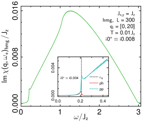
Figure 1: Spectrum, $\mathrm{Im}\chi({\bf q},\omega_{+})$, of energy density susceptibility versus $\omega$ at fixed small ${\bf q}$, for low $T=0.01J_{z}\lesssim T^{\star}$, using Eq. (18) for homogeneous ground state gauge. System size $L^{2}=300\times 300$. Momentum ${\bf q}=2\pi/L\sum_{j=1,2}q_{ij}{\bf G}_{j}$. Inset: Blow up of low-$\omega$ region with reduced imaginary broadening $i0^{+}$. Dashed black: upper ph-continuum bound at $T=0$.

IV Results

We now discuss the density dynamics as obtained from the previous sections. First we consider the low-$T$ behavior, $T\lesssim T^{\star}$, using the homogeneous gauge ground state. As from Eq. (18), $\chi({\bf q},z)$ sums two channels: (i) particle-hole (ph) and (ii) particle-particle (pp) excitations. Their spectral support is $0{<}{|}\omega{|}{<}\epsilon_{\tilde{{\bf q}}}$ for (ph) and $\epsilon_{\tilde{{\bf q}}}{<}{|}\omega{|}{\lesssim}\max(2\epsilon_{{\bf k}}){=}3J$ at ${|}{\bf q}{|}{\ll}1$ for (pp), where $\tilde{{\bf q}}{=}{\bf q}{+}{\bf k}_{D}$ refers to the wave vector with respect to the location of the Dirac cone. A typical spectrum $\mathrm{Im}\chi({\bf q},\omega_{+})$ is shown in Fig. 1 at small, albeit finite ${\bf q}$. The inset depicts a blowup of the low-$\omega$ region dissecting the spectrum into its ph and pp contributions. While the imaginary broadening in the inset is already reduced such that finite size oscillations start to show, the pp-channel still exhibits some weight below its cut-off at $\epsilon_{\tilde{{\bf q}}}\simeq 0.208J_{z}$. This will vanish as $\mathrm{Im}z\rightarrow 0$. For the ph-channel however, the spectral weight in this energy range is not a finite size effect. Due to the Dirac cone, the Fermi volume shrinks to zero in the Kitaev model as $T{\rightarrow}0$, i.e., occupied states only stem from a small patch with $\epsilon_{{\bf k}}\lesssim T$ around the Dirac cone. Therefore, the weight of the ph-channel decreases rapidly to zero as $T{\rightarrow}0$. In this regime and for small ${\bf q}$, because of the linear fermion dispersion close to the cones, only a narrow strip of order $\omega\in[\max(0,\epsilon_{\tilde{{\bf q}}}-2T),\epsilon_{\tilde{{\bf q}}}]$ from the spectral support dominates the ph-continuum. At the upper edge of its support the ph DOS is singular. The inset of Fig. 1 is consistent with this, considering the finite system size and imaginary broadening used.

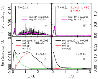
Figure 2: Spectrum, $\mathrm{Im}\chi({\bf q},\omega_{+})$, of energy density susceptibility versus $\omega$ at fixed small ${\bf q}=2\pi/L\sum_{j=1,2}q_{ij}{\bf G}_{j}$, contrasting homogeneous (a,b) versus random (c,d) gauge on all identical system sizes $L^{2}=60\times 60$ for two identical temperatures $T=0.1J_{z}$ (a,c) and $T=0.5J_{z}$ (b,d). Solid black, green, and red lines in panels (c,d): total, ph-, and pp-spectrum. Extended vertical gray ticks in panels (c,d): upper ph-continuum bound at $\boldsymbol{q}$ in homogeneous gauge. Imaginary smoothing $i0^{+}$ for homogeneous case, both, identical (solid black) and significantly larger than random gauge case (solid magenta). Note the different y-axis scales.

Regarding the pp-channel, the complete two-particle continuum is unoccupied and available for excited states as $T{\rightarrow}0$. This leads to the broad spectral hump seen in Fig. 1, which extends out to $\max(2\epsilon_{{\bf k}})=3J_{z}$, at $J_{x,y}=J_{z}$ and is two orders of magnitude larger than the ph-process at this temperature.

A fingerprint of potentially diffusive relaxation of density modes at finite momentum ${\bf q}$ is the near-linear behavior of $\mathrm{Im}\chi({\bf q},\omega_{+})\sim\chi_{\bf q}\,\omega/(Dq^{2})$ at small $\omega$. Definitely, this should neither be expected, nor is it observed in Fig. 1, since for $T\lesssim T^{\star}$, the density dynamics is set by coherent two-particle excitations of the Dirac fermions in the homogeneous gauge state.

For the remainder of this work, we therefore now turn to temperatures above the flux proliferation, i.e., $T\gtrsim T^{\star}$, using random gauge states. To begin, and in Fig. 2, we first describe the impact of the random gauges, by contrasting the dynamic density susceptibilities against each other with, and without random gauges, for otherwise identical system parameters, and for two different temperatures, $T=0.1$ and 0.5, in Figs. 2(a,c) and (b,d), respectively. Note, that while the linear system size is smaller by a factor of five with respect to Fig. 1, the wave vector has also been rescaled accordingly. Therefore these two figures can be compared directly. Obviously, in the homogeneous gauge, significant degeneracies, even on 60$\times$60 lattices, lead to visible discretization effects. Therefore, in Figs. 2(a,b) we include spectra with an imaginary broadening, increased relative to Figs. 2(c,d), for a better comparison with the latter.

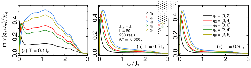
Figure 4: Spectrum of the normalized density susceptibility $\mathrm{Im}\chi({\bf q},\omega_{+})/\chi_{\boldsymbol{q}}$ in the random gauge state, with 200 realizations, versus $\omega$ for various temperatures $T/J_{z}=0.1,$ 0.5, and 0.9 in panels (a), (b), and (c), for various small momenta ${\bf q}=2\pi/L\sum_{j=1,2}q_{ij}{\bf G}_{j}$ within the small-$q$ region, inset panel (b), of the irreducible wedge of the BZ for $L^{2}=60\times 60$ sites and for imaginary broadening $i0^{+}$.

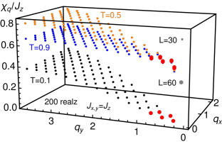
Figure 3: Static susceptibility $\chi_{\boldsymbol{q}}$ versus momentum in the random gauge state, with 200 realizations. Small solid dots: all of irreducible wedge of the BZ at $L^{2}=30\times 30$ for three temperatures $T/J_{z}=0.1$, 0.5, and 0.9 (black, orange, and blue). Big solid red dots, finite size effects: $\chi_{\boldsymbol{q}}$ at low$-q$ for $L^{2}=60\times 60$ and simultaneously $\boldsymbol{q}\in 30\times 30$ BZ.

Several features can be observed. First, while the ph-channel in the uniform gauge clearly displays the singular behavior at $\omega=\epsilon_{\tilde{{\bf q}}}$, mentioned earlier and visible because of the elevated temperatures, in the random gauge case, it displays a smooth peak. Second, as can be read of from the $y$-axis, the weight of the ph-channel strongly increases with increasing $T$. For the temperatures depicted, the pp-channel is much less $T$-dependent. Third, the ph-, versus the pp-contributions to $\mathrm{{Im}}\chi({\bf q},\omega_{+})$ cannot only be dissected in the uniform gauge by virtue of Eqs. (18), but also for the random gauge, Eq. (21) can be decomposed into addends with $\epsilon_{\sigma}\epsilon_{\rho}\gtrless 0$. This evidences, that in the latter case, the ph-spectrum changes completely. As is obvious from Figs. 2(c,d), the ph-channel spreads into a broad feature, extending over roughly the entire one-particle energy range. The pp-channel on the other hand seems less affected by the gauge disorder, with a shape qualitatively similar to that in the gauge ground state, as can be read off by comparing Figs. 2(a,c).

Most remarkably, for intermediate temperatures, as in Fig. 2(d) at $T/J_{z}=0.5$, the overall shape of the spectrum is very reminiscent of a diffusion-pole behavior at fixed momentum, i.e., $\mathrm{Im}\chi({\bf q},\omega)\propto\omega\Gamma/(\omega^{2}+\Gamma^{2})$, with some relaxation rate $\Gamma$. To clarify this in more detail, we therefore proceed and analyze $\chi({\bf q},z)$ in terms of the hydrodynamic expression Eq. (22).

To this end, we first extract the static susceptibility $\chi_{{\bf q}}$, performing the sum rule of Eq. (23) via numerical integration, using $\mathrm{{Im}}\chi({\bf q},z)$ from the corresponding random gauge states. The results are shown in Fig. 3, spanning an irreducible $\boldsymbol{q}$-wedge of the BZ. Since energy conservation renders the dynamic density response singular at $\boldsymbol{q}=\boldsymbol{0}$, this momentum will be excluded hereafter. Obviously $\chi_{{\bf q}}$ is a smooth and featureless function. The figure also contrasts 30$\times$30 against 60$\times$60 systems at selected momenta. The finite size effects are small.

Next, and in Fig. 4, we consider the global variation with momentum, of the normalized spectrum of the dynamical energy density susceptibility versus $\omega$. Since our focus is on the hydrodynamic regime, we remain with small momenta. These momenta are indicated on a fraction of an irreducible wedge of the BZ in Fig. 4(b). A spacing of $\mathrm{Mod}(2)$ of the momenta has been chosen to allow for later analysis of finite size effects in comparison to systems with a linear dimension smaller by a factor of 2. The spectra show significant changes with momentum. First, the low-$\omega$ contributions, which stem primarily from the ph-channel show a broadening of their support with increasing $|\boldsymbol{q}|$. Second, the spectral range of pp-excitations displays a global increase of weight with $|\boldsymbol{q}|$. Finally, at intermediate and elevated $T$ in Fig. 4(b) and (c), the former effect dominates the latter regarding the global shape of the spectrum.

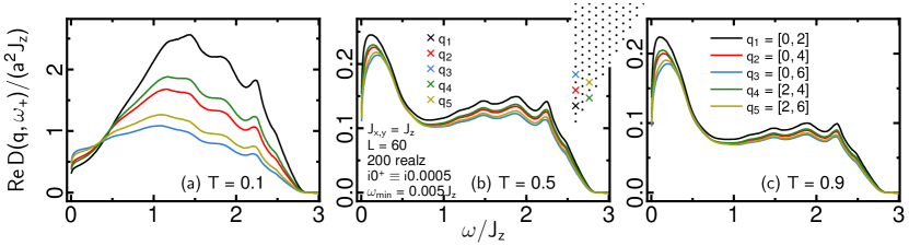
Figure 5: Real part of the diffusion kernel $\mathrm{Re}D({\bf q},\omega_{+})$ in the random gauge state, with 200 realizations, versus $\omega\geq.005J_{z}$ for various temperatures $T/J_{z}=0.1,$ 0.5, and 0.9 in panels (a), (b), and (c), for various small momenta ${\bf q}=2\pi/L\sum_{j=1,2}q_{ij}{\bf G}_{j}$ within the small-$q$ region, inset panel (b), of the irreducible wedge of the BZ for $L^{2}=60\times 60$ sites and for imaginary broadening $i0^{+}$.

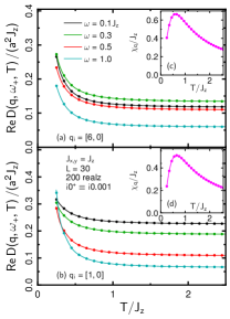
Figure 6: Real part of the diffusion kernel $\mathrm{Re}D({\bf q},\omega_{+},T)$ in the random gauge state, with 200 realizations, versus $T/J_{z}$ at ${\bf q}=2\pi/L\sum_{j=1,2}q_{ij}{\bf G}_{j}$ at (a) $\boldsymbol{q}_{i}=[6,0]$ and (b) $[1,0]$, and various fixed energies $\omega$, for $L^{2}=30\times 30$ sites and imaginary broadening $i0^{+}$. Insets (c,d): static susceptibility $\chi_{\boldsymbol{q}}(T)$ versus $T/J_{z}$ at identical $L$ and $\boldsymbol{q}$.

Now we extract the diffusion kernel $D({\bf q},\omega_{+})$ as in Eq. (24). Its real part is depicted in Fig. 5 versus $\omega$ for identical momenta and temperatures as in Fig. 4. Clearly, at low $T$, Fig. 5(a), the diffusion kernel displays significant $\boldsymbol{q}$-dependence, implying that the energy currents are not proportional to the gradient $\nabla_{\boldsymbol{l}}h_{\boldsymbol{l}}$ of the energy density and therefore a simply hydrodynamic picture is not applicable. In contrast to that, at intermediate and high $T$, Fig. 5(b) and (c), the diffusion kernel is approximately momentum independent $\mathrm{Re}D(|{\bf q}|\ll 1,\omega_{+})\simeq\mathrm{Re}D(\omega_{+})$. This is consistent with Fick’s law regarding $\boldsymbol{q}$-scaling. However, the diffusion process remains retarded, although not very strong, displaying a shoulder in the pp-range and a peak at low $\omega$ in the ph-range.

As $\omega/J_{z}\rightarrow 0$, the numerical accuracy of the transform Eq. (24), comprising small numbers in the numerator and denominator, is an issue with respect to system size and imaginary broadening and we have to remain with $\omega\geq\omega_{\mathrm{min}}=0.005J_{z}$ for the parameters used. See also the discussion of Fig. 7. In view of the steep slope in this regime, it may be that on any finite system $\mathrm{Re}D(|{\bf q}|\ll 1,\omega=0)$ vanishes singularly below the unphysically small energy scale $\omega_{\mathrm{min}}$, while in the thermodynamic limit $\mathrm{Re}D(|{\bf q}|\ll 1,\omega=0)$ is of the order of the low-energy peak height. This behavior is very reminiscent of similar findings for the thermal conductivity, see Ref. Metavitsiadis2017 and App. A. For $\omega/J_{z}\gtrsim 2.8$, the spectral support terminates and the diffusion kernel turns purely imaginary $\propto\omega^{-1}$. In conclusion, at not too low temperatures and not too short time scales, gauge disorder in the Kitaev magnet leads to an energy density dynamics, very similar to conventional diffusion, regarding its momentum scaling, with, however, some retardation remaining. This should be contrasted with the underlying spin model being a translationally invariant system.

Turning to the temperature dependence, we consider two representative momenta $\boldsymbol{q}$ and several energies. The corresponding diffusion kernel $\mathrm{Re}D({\bf q},\omega_{+})$ and the static susceptibility $\chi_{\boldsymbol{q}}$ are shown versus $T$ in Figs. 6(a), (b) and (c), (d), respectively. The temperature range has been truncated deliberately to $T/J_{z}\gtrsim 0.25$, since below such temperatures, and from the ${\bf q}$-scaling in Fig. 5 the density dynamics is far from hydrodynamic. The figure clearly demonstrates, that for $T/J_{z}\gtrsim 0.5$, the diffusion kernel rapidly settles onto some almost constant value, set by energy and momentum. This is consistent with Fig. 5, which displays only weak overall change between the diffusion kernels for the two temperatures of panels (b) and (c). As a consequence, the global $T$-dependence of $\chi(\boldsymbol{q},z)$ is essentially set by the static energy susceptibility. As the insets show, the latter exhibits a maximum in the vicinity of $T/J_{z}\sim 1$. For $T/J_{z}\gg 1$, $\chi_{{\bf q}}$ approaches its classical limit, decaying $\propto T^{-1}$, which can also be read of from Eqs. (23,21). Such behavior is typical also for other static susceptibilities of spin systems.

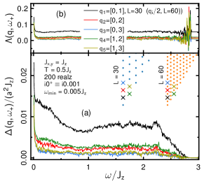
Figure 7: (a) Absolute and (b) relative difference of real part of the diffusion kernel $\mathrm{Re}D({\bf q},\omega_{+})$ in the random gauge state, with 200 realizations, versus $\omega\geq 0.005J_{z}$ at $T/J_{z}=0.5$, for various small momenta ${\bf q}=2\pi/L\sum_{j=1,2}q_{ij}{\bf G}_{j}$ on $L^{2}=30\times 30$ and $\boldsymbol{q}_{i}\rightarrow 2\boldsymbol{q}_{i}$ on $L^{2}=60\times 60$, within the small-$q$ region of insets panel (a), of the irreducible wedge of the BZ and for imaginary broadening $i0^{+}$.

In closing, we provide some measure of the finite size effects involved in our calculations. To this end we consider both, the absolute and the relative difference between the diffusion kernels, $\Delta({\bf q},\omega)=|\mathrm{Re}[D_{30{\times}30}({\bf q},\omega_{+})-D_{60{\times}60}({\bf q},\omega_{+})]|$ and $\Lambda({\bf q},\omega)=2\Delta({\bf q},\omega)/|\mathrm{Re}[D_{30{\times}30}({\bf q},\omega_{+})+D_{60{\times}60}({\bf q},\omega_{+})]|$, respectively, on $N=30{\times}30$ and $60{\times}60$ site systems, for identical wave vectors. Regarding the latter, this implies a factor of $2$ difference between their integer representation in terms of ${\bf G}_{1,2}$. The differences are shown in Fig. 7. They display statistical noise from the finite number of random gauge realizations and remain acceptably small for all $\omega$. Only for $0\approx\omega\ll 0.01$, where $\Lambda({\bf q},\omega)$ is of $O(10\%)$, the error is not of finite size, or statistical origin, but rather stems from the systematic numerical inaccuracies, mentioned in the preceding, of the denominator in Eq. (24) with $\chi({\bf q},\omega_{+})$ obtained from Eq. (21) as $\omega\rightarrow 0$. In turn, $D({\bf q},\omega_{+})$ at very low $0\approx\omega\ll 0.01$ may be inacurate by $\sim 10\%$. As to be expected, the actual finite size errors are largest for the smallest wave vector.

V Summary

In summary, above an intermediate temperature scale $T\sim 0.5J$, which is still well below the classical limit, the energy density in Kitaev magnets at finite momentum relaxes remarkably similar to diffusion in random media, with, however, a clearly notable difference. Namely, while the momentum scaling is practically hydrodynamic $\propto q^{2}$, the diffusion kernel is not completely energy independent, i.e., it displays some retardation within its support. The origin of the latter can be traced back to the presence of two distinct relaxation channels for the energy density, comprising particle-hole and particle-particle excitations of the Dirac fermions. Both propagate in a strongly disordered landscape, created by thermally induced gauge excitations. Their combined effect, however, does not lead to a constant diffusion rate. At extremely low energies we observe a dip in the diffusion kernel. This is consistent with similar claims for the dynamical thermal conductivity, to which we find that our results connect consistently via generalized Einstein relations. Future analysis, focusing on the real space, instead of the momentum dependence of energy-density relaxation could be interesting in order to predict finite temperature quench dynamics.

Acknowledgments: This work has been supported in part by the DFG through project A02 of SFB 1143 (project-id 247310070), by Nds. QUANOMET (project NP-2), and by the National Science Foundation under Grant No. NSF PHY-1748958. W.B. also acknowledges kind hospitality of the PSM, Dresden.

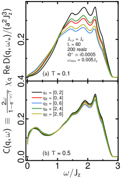
Figure 8: Momentum evolution of Einstein relation for current correlation function in the random gauge state, with 200 realizations, versus $\omega\geq 0.005J_{z}$ for $T/J_{z}=0.1,$ and 0.5 in panels (a) and (b), for various small momenta ${\bf q}=2\pi/L\sum_{j=1,2}q_{ij}{\bf G}_{j}$ within the small-$q$ region identical to Fig. 5, for $L^{2}=60\times 60$ sites and for imaginary broadening $i0^{+}$.

Appendix A Current correlation functions

In the limit of $\boldsymbol{q}\rightarrow\boldsymbol{0}$ one may speculate, that the dynamical energy-density diffusion kernel is related to the dynamical energy-current correlation function via a generalized Einstein relation. The zero momentum current correlation function has been considered in Ref. Metavitsiadis2017 . For completeness sake, we now clarify a relation of the latter quantity to the present work. From Mori-Zwanzig’s memory function method we have

$$\frac{1}{z}(\chi_{{\bf q}}-\chi({\bf q},z))=\frac{1}{z-M({\bf q},z)\frac{1}{\chi_{{\bf q}}}}\chi_{{\bf q}}\,,$$ (25)

where $M({\bf q},z)=\langle Lh_{{\bf q}}|(z-QL)^{-1}QLh_{{\bf q}}\rangle$ is the memory function. $L$ is the Liouville operator $LA=[H,A]$ and $\langle A|B\rangle=\int_{0}^{\beta}\langle A^{+}(\lambda)B\rangle d\lambda-\beta\langle A^{+}\rangle\langle B\rangle$ is Mori’s scalar product with $A(\lambda)=e^{\lambda H}Ae^{-\lambda H}=e^{\lambda L}A$ and $\beta=1/T$ is the inverse temperature. $\chi_{{\bf q}}$ is the isothermal energy susceptibility $\chi_{{\bf q}}=\langle h_{{\bf q}}|h_{{\bf q}}\rangle$ and $Q$ is a projector perpendicular to the energy density, which is formulated using Mori’s product as $Q=1-|h_{{\bf q}}\rangle\chi_{{\bf q}}^{-1}\langle h_{{\bf q}}|$. We emphasize, that Eq. (25) is not a “high-frequency”, or “slow-mode” approximation. It is a rigorous statement. Due to time-reversal invariance, $QLh_{{\bf q}}=Lh_{{\bf q}}$ Forster1975 . Moreover, using the continuity equation in the hydrodynamic regime, i.e., discarding the lattice structure, we have $Lh_{{\bf q}}=-{\bf q}\cdot{\bf j_{{\bf q}}}$, where ${\bf j_{{\bf q}}}$ is the energy current. Altogether

$$i\chi_{{\bf q}}D({\bf q},z)=\sum_{\mu\nu}e_{\boldsymbol{q}\mu}e_{\boldsymbol{q}\nu}\langle j_{\boldsymbol{q}\mu}|\frac{1}{z-QL}j_{\boldsymbol{q}\nu}\rangle\,,$$ (26)

where $\boldsymbol{e}_{\boldsymbol{q}\mu}$ are the components of the unit vector into $\boldsymbol{q}$-direction. While for arbitrary $\boldsymbol{q}$ the right hand side refers to a so-called current relaxation-function with a dynamics governed by a projected Liouville operator $QL$, for $\boldsymbol{q}\rightarrow\boldsymbol{0}$, one finds that $\lim_{\boldsymbol{q}\rightarrow\boldsymbol{0}}\langle j_{\boldsymbol{q}\mu}|(z-QL)^{-1}j_{\boldsymbol{q}\nu}\rangle=\langle j_{\boldsymbol{0}\mu}|(z-L)^{-1}j_{\boldsymbol{0}\nu}\rangle$ Forster1975 , which is the genuine current relaxation-function comprising the complete Liouvillean dynamics. This turns Eq. (26) into an Einstein relation for $\boldsymbol{q}\rightarrow\boldsymbol{0}$. Finally, the spectrum of the current relaxation-function can be related to that of a standard current correlation-function $C_{\mu\nu}(t)=\langle j_{\boldsymbol{0}\mu}(t)j_{\boldsymbol{0}\nu}\rangle$ by the Kubo relation and the fluctuation dissipation theorem

$$\frac{2\omega}{1-e^{\omega/T}}\lim_{\boldsymbol{q}\rightarrow\boldsymbol{0}}\chi_{{\bf q}}\,\mathrm{Re}D({\bf q},z)=C(\omega)\,.$$ (27)

Here we have discarded questions of anisotropy. While the present work’s focus is on $\boldsymbol{q}\neq 0$, it is now very tempting to evaluate the left hand side of Eq. (27) using, e.g., the two temperatures of Fig. 5 (a,b) and to consider its evolution with momentum. This is shown in Fig. 8, which should be compared with Fig. 5 (b,d) of Ref. Metavitsiadis2017 . For this, and because of a different energy unit and normalization of spectral densities in the latter Ref., $T$ has to rescaled by $4$ and the y-axis by $4^{3}/\pi$. While the rescaled temperatures $T=0.25$ and $0.525$ of Ref. Metavitsiadis2017 are not absolutely identical to the ones we use, it is very satisfying to realize, that the limit $\boldsymbol{q}\rightarrow\boldsymbol{0}$ of Eq. (27), which can be anticipated from Fig. 8 is completely in line with Fig. 5 of Ref. Metavitsiadis2017 , including the dip at very low $\omega$. This is even more remarkable in view of the numerical representation and treatment of the Majorana fermions used in the present work and in Ref. Metavitsiadis2017 being decisively different.

References

- (1) A. V. Sologubenko, E. Felder, K. Giannò, H. R. Ott, A. Vietkine, and A. Revcolevschi, Phys. Rev. B 62, R6108 (2000).
- (2) T. Kawamata, N. Takahashi, T. Adachi, T. Noji, K. Kudo, N. Kobayashi, Y. Koike, J. Phys. Soc. Jp. 77, 034607 (2008).
- (3) N. Hlubek, P. Ribeiro, R. Saint-Martin, A. Revcolevschi, G. Roth, G. Behr, B. Büchner, C. Hess, Phys. Rev. B 81, 020405 (2010).
- (4) A. V. Sologubenko, K. Giannò, H. R. Ott, U. Ammerahl, and A. Revcolevschi, Phys. Rev. Lett. 84, 2714 (2000).
- (5) C. Hess, C. Baumann, U. Ammerahl, B. Büchner, F. Heidrich-Meisner, W. Brenig, and A. Revcolevschi, Phys. Rev. B 64, 184305 (2001).
- (6) X. Zotos, F. Naef, and P. Prelovsek, Phys. Rev. B 55, 11029 (1997).
- (7) Heidrich-Meisner, F., A. Honecker, D. C. Cabra, and W. Brenig, Phys. Rev. B 68, 134436 (2003).
- (8) Heidrich-Meisner, F., A. Honecker, D. C. Cabra, and W. Brenig, Phys. Rev. Lett. 92, 069703 (2004).
- (9) C. Hess, Eur. Phys. J. Spec. Top. 151, 73 (2007).
- (10) F. Heidrich-Meisner, A. Honecker, and W. Brenig, Eur. Phys. J. Special Topics 151, 135 (2007).
- (11) C. Hess, Phys. Rep. 811, 1 (2019).
- (12) B. Bertini, F. Heidrich-Meisner, C. Karrasch, T. Prosen, R. Steinigeweg, and M. Znidaric, arXiv:2003.03334
- (13) G. S. Dixon, Phys. Rev. B 21, 2851 (1980).
- (14) C. Hess, B. Büchner, U. Ammerahl, L. Colonescu, F. Heidrich-Meisner, W. Brenig, and A. Revcolevschi, Phys. Rev. Lett. 90, 197002 (2003).
- (15) S.P. Bayrakci, B. Keimer, and D.A. Tennant, arXiv:1302.6476
- (16) A. L. Chernyshev and Wolfram, Phys. Rev. B 92, 054409 (2015).
- (17) L. Balents, Nature 464, 199-208 (2010).
- (18) L. Savary and L. Balents, Rep. Prog. Phys. 80, 016502 (2017).
- (19) M. Yamashita, N. Nakata, Y. Senshu, M. Nagata, H. M. Yamamoto, R. Kato, T. Shibauchi, and Y. Matsuda, Science 328, 1246 (2010).
- (20) P. Bourgeois-Hope, F. Laliberté, E. Lefrançois, G. Grissonnanche, S. R. de Cotret, R. Gordon, S. Kitou, H. Sawa, H. Cui, R. Kato, L. Taillefer, and N. Doiron-Leyraud, Phys. Rev. X 9, 041051 (2019).
- (21) J. M. Ni, B. L. Pan, B. Q. Song, Y. Y. Huang, J. Y. Zeng, Y. J. Yu, E. J. Cheng, L. S. Wang, D. Z. Dai, R. Kato, and S. Y. Li, Phys. Rev. Lett. 123, 247204 (2019).
- (22) G. Kolland, O. Breunig, M. Valldor, M. Hiertz, J. Frielingsdorf, and T. Lorenz, Phys. Rev. B 86, 060402(R) (2012).
- (23) W. H. Toews, S. S. Zhang, K. A. Ross, H. A. Dabkowska, B. D. Gaulin, and R. W. Hill, Phys. Rev. Lett. 110, 217209 (2013).
- (24) Y. Tokiwa, T. Yamashita, D. Terazawa, K. Kimura, Y. Kasahara, T. Onishi, Y. Kato, M. Halim, P. Gegenwart, T. Shibauchi, S. Nakatsuji, E.-G. Moon, and Y. Matsuda, J. Phys. Soc. Jpn. 87, 064702 (2018).
- (25) M. Hirschberger, R. Chisnell, Y. S. Lee, and N. P. Ong, Phys. Rev. Lett. 115, 106603 (2015).
- (26) D. Watanabe, K. Sugii, M. Shimozawa, Y. Suzuki, T. Yajima, H. Ishikawa, Z. Hiroi, T. Shibauchi, Y. Matsuda, and M. Yamashita, PNAS 113, 8653 (2016).
- (27) M. Yamashita, M. Akazawa, M. Shimozawa, T. Shibauchi, Y. Matsuda, H. Ishikawa, T. Yajima, Z. Hiroi, M. Oda, H. Yoshida, H.-Y. Lee, J. H. Han, and N. Kawashima, J. Phys.: Condens. Matter 32, 074001 (2019).
- (28) M. Hirschberger, J. W. Krizan, R. J. Cava, and N. P. Ong, Science 348, 106 (2015).
- (29) A. Kitaev, Ann. Phys. (N.Y.) 321, 2 (2006).
- (30) X.-Y. Feng, G.-M. Zhang, and T. Xiang, Phys. Rev. Lett. 98, 087204 (2007).
- (31) H.-D. Chen and Z. Nussinov, J. Phys. A: Math. Theor. 41, 075001 (2008).
- (32) Z. Nussinov and G. Ortiz, Phys. Rev. B 79, 214440 (2009).
- (33) S. Mandal, R. Shankar and G. Baskaran, J. Phys. A: Math. Theor. 45, 335304 (2012).
- (34) K. W. Plumb, J. P. Clancy, L. J. Sandilands, V. V. Shankar, Y. F. Hu, K. S. Burch, H.-Y. Kee, and Y.-J. Kim, Phys. Rev. B 90, 041112 (2014).
- (35) S. Trebst, Kitaev Materials, Lecture Notes of the 48th IFF Spring School 2017, S. Blügel, Y. Mokrousov, T. Schäpers, Y. Ando (Eds.), ISBN 978-3-95806-202-3
- (36) A. Banerjee, C. A. Bridges, J. Q. Yan, A. A. Aczel, L. Li, M. B. Stone, G. E. Granroth, M. D. Lumsden, Y. Yiu, J. Knolle, S. Bhattacharjee, D. L. Kovrizhin, R. Moessner, D. A. Tennant, D. G. Mandrus, and S. E. Nagler, Nat. Mater. 15, 733 (2016).
- (37) A. Banerjee, J. Yan, J. Knolle, C. A. Bridges, M. B. Stone, M. D. Lumsden, D. G. Mandrus, D. A. Tennant, R. Moessner, and S. E. Nagler, Science 356, 6342 (2017).
- (38) A. Banerjee, P. Lampen-Kelley, J. Knolle, C. Balz, A. A. Aczel, B. Winn, Y. Liu, D. Pajerowski, J. Yan, C. A. Bridges, A. T. Savici, B. C. Chakoumakos, M. D. Lumsden, D. A. Tennant, R. Moessner, D. G. Mandrus, and S. E. Nagler, Nat. Part. J. Quantum Mater. 3, 8 (2018).
- (39) J. Knolle, G.W. Chern, D.L. Kovrizhin, R. Moessner, and N.B. Perkins, Phys. Rev. Lett. 113, 187201 (2014).
- (40) D. Wulferding, Y. Choi, S.-H. Do, C. H. Lee, P. Lemmens, C. Faugeras, Y. Gallais, and K.-Y. Choi, Nat Commun 11, 1 (2020).
- (41) S.-H. Baek, S.-H. Do, K. Y. Choi, Y.S. Kwon, A.U.B. Wolter, S. Nishimoto, J. van den Brink, and B. Büchner, Phys. Rev. Lett. 119, 037201 (2017).
- (42) J. Zheng, K. Ran, T. Li, J. Wang, P. Wang, B. Liu, Z.-X. Liu, B. Normand, J. Wen, and W. Yu, Phys. Rev. Lett. 119, 227208 (2017).
- (43) D. Hirobe, M. Sato, Y. Shiomi, H. Tanaka, and E. Saitoh, Phys. Rev.~B 95, 241112 (2017).
- (44) I.A. Leahy, C.A. Pocs, P.E. Siegfried, D. Graf, S.-H. Do, K.-Y. Choi, B. Normand, and M. Lee, Phys. Rev. Lett. 118, 187203 (2017).
- (45) R. Hentrich, A. U. B. Wolter, X. Zotos, W. Brenig, D. Nowak, A. Isaeva, T. Doert, A. Banerjee, P. Lampen-Kelley, D. G. Mandrus, S. E. Nagler, J. Sears, Y.-J. Kim, B. Büchner, C. Hess, Phys. Rev. Lett. 120, 117204 (2018).
- (46) Y. J. Yu, Y. Xu, K. J. Ran, J. M. Ni, Y. Y. Huang, J. H. Wang, J. S. Wen, and A. Y. Li, Phys. Rev. Lett. 120, 067202 (2018).
- (47) Alexandros Metavitsiadis and Wolfram Brenig, Phys. Rev. B 101, 035103 (2020).
- (48) Y. Kasahara, T. Ohnishi, Y. Mizukami, O. Tanaka, S. Ma, K. Sugii, N. Kurita, H. Tanaka, J. Nasu, Y. Motome, T. Shibauchi, and Y. Matsuda, Nature 559, 227 (2018).
- (49) T. Yokoi, S. Ma, Y. Kasahara, S. Kasahara, T. Shibauchi, N. Kurita, H. Tanaka, J. Nasu, Y. Motome, C. Hickey, S. Trebst, and Y. Matsuda, ArXiv:2001.01899 [Cond-Mat] (2020).
- (50) A. Metavitsiadis and W. Brenig, Rev. B 96, 041115(R) (2017).
- (51) J. Nasu, J. Yoshitake, and Y. Motome, Phys. Rev. Lett. 119, 127204 (2017).
- (52) A. Metavitsiadis, A. Pidatella, and W. Brenig, Phys. Rev. B 96, 205121 (2017).
- (53) A. Pidatella, A. Metavitsiadis, and W. Brenig Phys. Rev. B 99, 075141 (2019).
- (54) A. Metavitsiadis, C. Psaroudaki, and W. Brenig, Phys. Rev. B 99, 205129 (2019).
- (55) A. Metavitsiadis and W. Brenig, ArXiv:2009.04467 [Cond-Mat] (2020).
- (56) J. Nasu, M. Udagawa, and Y. Motome, Phys. Rev. B 92, 115122 (2015).
- (57) D. Forster, Hydrodynamic Fluctuations, Broken Symmetry, and Correlation Functions, (Benjamin, New York, 1975).