Inspecting the Cepheid distance ladder:
The Hubble Space Telescope distance to the SNIa host galaxy NGC 5584

Abstract

The current tension between the direct and the early Universe measurements of the Hubble Constant, $H_{0}$, requires detailed scrutiny of all the data and methods used in the studies on both sides of the debate. The Cepheids in the type Ia supernova (SNIa) host galaxy NGC 5584 played a key role in the local measurement of $H_{0}$. The SH0ES project used the observations of this galaxy to derive a relation between Cepheids’ periods and ratios of their amplitudes in different optical bands of the Hubble Space Telescope (HST), and used these relations to analyse the light curves of the Cepheids in around half of the current sample of local SNIa host galaxies. In this work, we present an independent detailed analysis of the Cepheids in NGC 5584. We employ different tools for our photometric analysis and a completely different method for our light curve analysis, and we do not find a systematic difference between our period and mean magnitude measurements compared to those reported by SH0ES. By adopting a period-luminosity relation calibrated by the Cepheids in the Milky Way, we measure a distance modulus $\mu=31.810\pm 0.047$ (mag) which is in agreement with $\mu=31.786\pm 0.046$ (mag) measured by SH0ES. In addition, the relations we find between periods and amplitude ratios of the Cepheids in NGC 5584 are significantly tighter than those of SH0ES and their potential impact on the direct $H_{0}$ measurement will be investigated in future studies.

1 Introduction

The current expansion rate of the Universe, known as the Hubble constant or $H_{0}$, is one of the fundamental parameters of the standard model of cosmology and of any viable cosmological model. A few decades after the initial estimate of around 500 km s^-1Mpc^-1 by Hubble (1929), $H_{0}$ became a place for debate with values either $\approx 100$ km s^-1Mpc^-1(e.g. van den Bergh, 1970; de Vaucouleurs, 1972) or $\approx 50$ km s^-1Mpc^-1(e.g. Sandage & Tammann, 1975). The debate was finally settled after the findings of the HST $H_{0}$ Key Project whose final results was $H_{0}=72\pm 8$ km s^-1Mpc^-1(Freedman et al., 2001). This value was found to be in agreement with the subsequent results from the observations of the Cosmic Microwave Background (CMB) by the Wilkinson Microwave Anisotropy Probe (WMAP, e.g. Spergel et al., 2003) based on the standard Lamda-Cold-Dark-Matter ($\Lambda$CDM) model. However, in the recent years and with the improved precision of the measurements of $H_{0}$, a significant tension has again risen this time between the so called early-Universe cosmology-dependent approaches finding $H_{0}\approx 67$ km s^-1Mpc^-1and late-Universe direct measurements mostly finding $H_{0}\approx 73$ km s^-1Mpc^-1.

On the one hand, using the precise observations of the CMB from the Planck satellite, Planck Collaboration et al. (2018) concluded that the $\Lambda$CDM provides an excellent explanation of the CMB data and reported a model-dependent prediction of the Hubble constant $H_{0}=67.4\pm 0.5$ km s^-1Mpc^-1. This result is in good agreement with other early Universe measurements. For example, by combining baryon acoustic oscillation (BAO) and Big Bang nucleosynthesis (BBN) data, Addison et al. (2018) reported a CMB-independent value of $H_{0}=66.98\pm 1.18$ km s^-1Mpc^-1, and by combining BBN and BAO data with galaxy clustering and weak lensing data, the Dark Energy Survey reported $H_{0}=67.4^{+1.1}_{-1.2}$ km s^-1Mpc^-1(Abbott et al., 2018). In a recent study and based on new high resolution CMB observations from the Atacama Cosmology Telescope, Aiola et al. (2020) reported $H_{0}=67.9\pm 1.5$ km s^-1Mpc^-1, consistent with previous early Universe results. All these results are based on the $\Lambda$CDM model.

On the other hand, the SH0ES (Supernovae $H_{0}$ for the Equation of State) project, that uses the Cepheid calibrated SNeIa data, finds a significantly higher locally measured $H_{0}$ value. Cepheids are one of the most reliable distance indicators and, using more than a decade of observations(see e.g. Riess et al., 2005), the SH0ES project measures $H_{0}=73.5\pm 1.4$ km s^-1Mpc^-1for the Hubble constant (Riess et al., 2019; Riess, 2019). This is one of the most precise determinations of $H_{0}$ and is in more than $4\sigma$ tension with the early-Universe results.

There are also other direct but Cepheid-independent methods for measuring $H_{0}$. Using time-delay data of gravitationally lensed quasars, the H0LiCOW (H0 lenses in COSMOGRAIL’s Wellspring) project reported $H_{0}=73.3^{+1.7}_{-1.8}$ km s^-1Mpc^-1(Wong et al., 2020). In another gravitational lensing study, Birrer et al. (2020) employed a different lens mass profile modeling approach and found $H_{0}=67.4^{+4.1}_{-3.2}$ km s^-1Mpc^-1and $H_{0}=74.5^{+5.6}_{-6.1}$ km s^-1Mpc^-1using two different data sets. Using yet another independent method of geometric distance measurements to megamaser-hosting galaxies, Pesce et al. (2020) reported $H_{0}=73.9\pm 3.0$ km s^-1Mpc^-1. Another late Universe method to measure the $H_{0}$ is to calibrate the SNeIa with the tip of the red giant branch (TRGB), using which the Carnegie-Chicago Hubble Program (CCHP) found $H_{0}=69.8\pm 1.4$ km s^-1Mpc^-1(Freedman et al., 2019).

Although some late Universe results are in agreement with those from early Universe approaches, the absolute majority of direct methods find $H_{0}$ values larger than the early Universe model-dependent methods, and currently different combinations of the late Universe measurements are in 4 to $6\sigma$ tension with the early Universe $\Lambda$CDM predictions (Verde et al., 2019; Riess, 2019), and removing any one method does not appear to resolve the tension. In fact, the general consistency of the direct methods on the one hand, and of those of the early-Universe methods on the other hand, significantly reduces the possibility that systematics in one method, data, or analysis would solve this problem.

However, since the persistence of the $H_{0}$ tension would mean the failure of the base $\Lambda$CDM model, and given the generally understood success of the $\Lambda$CDM in explaining the CMB and the large-scale structure data, it is absolutely necessary to not only take different approaches for measuring $H_{0}$, but also, as emphasized by Riess et al. (2020), to scrutinize in detail all the data, methods, and the studies that have led to this cosmic discordance.

The main three rungs of the Cepheid distance ladder are i) calibration of the period-luminosity relation using geometric distance measurements to nearby Cepheids, ii) calibration of the SNIa absolute magnitude using Cepheids in SNIa host galaxies out to around 40 Mpc, and iii) using SNIa out to redshift 0.15 to measure $H_{0}$.

On the first rung, different studies (e.g. Nardetto, 2018; Borgniet et al., 2019; Kervella et al., 2019b; Gallenne et al., 2019; Anderson, 2019; Hocdé et al., 2020a, b; Musella et al., 2020) have focused on enhancing our understanding of the different properties of Cepheid variables, and in a recent study, Breuval et al. (2020) presented a new calibration of PL relation for Milky Way Cepheids using their companion parallaxes from Gaia (Kervella et al., 2019a). In addition, the high precision measurement of the distance to the Large Magellanic Cloud (LMC) by Pietrzyński et al. (2019) provides an accurate calibration of the Cepheid period-luminosity relation in this satellite galaxy of the Milky Way.

On the third rung, the impact of SNeIa environment (Roman et al., 2018) and in particular that of the star formation rate (Rigault et al., 2015) of their host galaxies on distance measurements has been investigated. Jones et al. (2018), however, concludes that the environmental dependency of SNeIa properties have negligible effect on the $H_{0}$ measurements. Dhawan et al. (2018) and Burns et al. (2018) used near-infrared observations, where SNeIa luminosity variations and extinction by dust are less than in the optical observations, and concluded that the $H_{0}$ tension is likely not caused by systematics like dust extinction or SNeIa host galaxy mass. Also, Hamuy et al. (2020) reported that different methods for standardization of SNeIa light curves yield consistent results with a small standard deviation, concluding that SNeIa are robust calibrators of the third rung.

In this study, we scrutinize the second rung, that is, the Cepheid calibration of SNeIa host galaxies. This intermediate rung plays the important role of connecting the geometric distance calibrations of the ladder to the cosmic scales. Therefore, it is vital to also investigate the observations and analysis involved in the second rung of the Cepheid distance ladder independently of SH0ES that has so far been the only program undertaking this effort. Riess et al. (2016, hereafter R16) used HST data to measure the Cepheid distances to 19 SNIa host galaxies for the calibration of the luminosity of larger distance SNIa. R16 presents the near-infrared (NIR) observations, whereas a companion paper by Hoffmann et al. (2016, hereafter H16) reports the complete optical observations of Cepheid variables in these SNIa host galaxies. Out of these 19 galaxies, 10 have been observed in the earlier stages of the SH0ES project (Riess et al., 2009) and with older HST instruments, i.e. NICMOS and WFPC2, using F555W (V), F814W (I), and F160W (H) bands for measuring mean magnitudes and periods of their Cepheid variables. However, for 9 out of 19 of these galaxies, the photometric time series necessary for identifying the Cepheids, measuring their light curves and estimating their periods, have been obtained using the wide band HST F350LP filter available on WFC3/UVIS. The wavelength range of this so called ”white light” filter covers those of V and I bands, hence is suitable for the detection of faint sources. The 9 galaxies mentioned above currently have much fewer random phase observations in V and I bands, not sufficient for light curve analysis. NGC 5584, however, has time series observations in all these three bands. Using the data of this galaxy, the SH0ES team obtained a relation between the periods of the Cepheids and the ratio of their amplitudes in V and I relative to those in F350LP band. Then, assuming that these relations derived from NGC 5584 also hold in other SNIa host galaxies, the SH0ES project correct for the effect of random phase observations of Cepheids in the galaxies with few V and I observations. Therefore, the Cepheids in the galaxy NGC 5584 played a key role in obtaining the periods and mean magnitudes of the Cepheids in almost half of the current SH0ES sample of SNeIa host galaxies, and in turn in the final measurement of $H_{0}$.

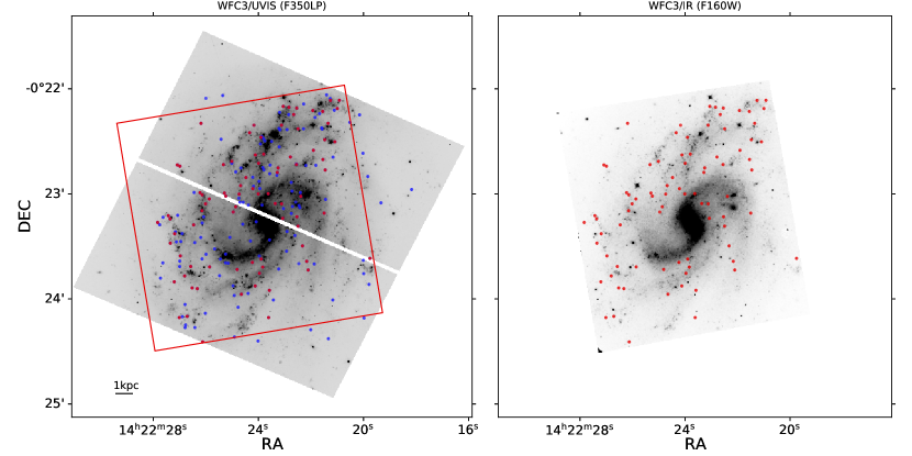
Figure 1: Examples of the HST images from the NGC 5584 in the F350LP (left) and F160W (right) bands. The former image is from the WFC3/UVIS which has two mosaics of 4096 $\times$ 2051 pixels separated by a 35-pixel ($\approx 1.4\arcsec$) gap, and the latter is from the WFC3/IR with a dimension of 1014 pix $\times$ 1014 pix. The red square outline on the left panel shows the WFC3/IR field of view on this galaxy. The scattered dots show the positions of the Cepheids, the ones with red color are identified in both optical and infrared, while the ones with blue are identified only in the optical bands. On both panels North is up and East is to the left.

.

For our inspection, we use the same observations of NGC 5584 that were used by SH0ES. Hence, this work is not a complete reproduction of the original experiment, since we do not repeat the observations themselves. However, where possible, we intentionally explore different numerical methods and tools than those used by SH0ES to provide an independent insight to the $H_{0}$ problem. The goal of this work is to inspect the foundations of the Cepheid distance scale, independently of any input on our analysis from the SH0ES team.

This paper is organized as follows. In Section 2, we briefly outline the method. Section 3 presents a full description of the data. We describe our analysis in Section 4, present our results in Section 5, and finally conclude in Section 6.

2 Method

A standard approach for distance measurements using the Cepheid variables (Leavitt & Pickering, 1912) is to use reddening-free ”Wesenheit” index (Madore, 1982) in the $H$ band defined by R16 as

$$W_{H}=H-R_{H}(V-I)$$ (1)

where $H$, $V$, and $I$ are mean magnitude of the Cepheids in F160W, F555W, and F814W, respectively. In our analysis, we adopt $R_{H}=0.386$ which is derived from Cardelli et al. (1989) and Fitzpatrick (1999), and is also adopted by e.g. Riess et al. (2019), Bentz et al. (2019), and Breuval et al. (2020). The distance to a nearby SNIa host galaxy can be measured by obtaining the relation between the pulsation period and $W_{H}$ of its identified Cepheids, and by adopting a $W_{H}$ vs. period relation calibrated by the Cepheids in e.g. the Milky Way or the LMC. The observations of NGC 5584 for the measurements of periods and the mean magnitudes of its Cepheids in the above-mentioned bands are described in the next section.

3 Data

3.1 Archival Observations

We obtain the data of NGC 5584 from the Mikulski Archive for Space Telescopes (MAST) database. NGC 5584 has been observed by the Wide Field Camera 3 (WFC3) between January and April 2010 with the purpose of measuring a Cepheid distance to type Ia supernova SN 2007af hosted by this galaxy (PI: Adam Riess, Cycle: 17, Proposal ID: 11570). WFC3 has been installed on the HST in 2009 replacing the WFPC2. It has two imaging cameras: the UV/Visible channel (UVIS) and the near-infrared (IR) channel. UVIS has two mosaics of 2051 pixel $\times$ 4096 pixel each, a total field of view (FOV) of 162$\times$162 arcsec², and a resolution of 0.04 arcsec/pixel. The IR camera has a dimension of 1014 pix $\times$ 1014 pix with FOV 136$\times$123 arcsec², and a resolution of 0.13 arcsec/pixel.

NGC 5584 has been observed in 13 epochs (in total 45540 sec) in F555W band, 6 of which also accompanied by F814W observations (in total 14400 sec). In twelve of these epochs, this galaxy has also been observed in the F350LP band (in total 15000 sec). In addition, NGC 5584 has also been observed with WFC3/IR channel with the F160W or the H band in 2 epochs (in total 4929 sec).

3.2 Calibrations

In all cases, we obtain the calibrated cosmic-ray cleaned (i.e. the flc.fits files for WFC3/UVIS, and flt.fits files for the WFC3/IR observations) data provided by the MAST database. In the case of WFC3/UVIS, the flc.fits files are also corrected for the charge-transfer efficiency loss. We list the full information regarding these observations in Appendix D.

Similar to H16, we use the TweakReg software for image registration and alignment. For all the images of all the bands we achieve an alignment better than 0.1 pixels, the same precision is also reported by H16. We use the coordinates of the ”local standard stars” provided by H16 (see section 3.3 for more details on these stars) in order to have the same absolute astrometry as theirs. This provides an exact identification of the Cepheids using the RA and DEC reported by H16.

Each observation epoch consists of multiple exposures. For example, 11 out of 13 epochs in F555W bands consist of six different exposures, and the other two, consist of four different exposures (see Appendix D). We use the AstroDrizzle software${}^{\ref{drizzlepac}}$ to combine all the exposures of each epoch (and of the same filter) to obtain final distortion-corrected drizzled science images for the purpose of our analysis.

Figure 1 shows examples of UVIS and IR images of the NGC 5584.

3.3 The Cepheids in NGC 5584

After performing Point-Spread Function (PSF) photometry for all the sources in the galaxy image, H16 uses the Welch & Stetson (1993) variability index to identify variable objects. This procedure requires comparing fluxes of each epochs with non-variable sources. A list of visually inspected such ”local standard stars” is provided by H16 in their table 3. H16 fits all variable objects with Cepheid light curve templates from Yoachim et al. (2009), which have been generated for V and I bands and by a combination of Fourier decomposition and principal component analysis from a sample of Cepheids in the MW, the LMC, and the Small Magellanic Cloud. After template fitting, H16 visually inspects the six best solution for all the variables, and rejects the variables that are poorly fitted. The details on further criteria that H16 applied to get to their final Cepheid sample are presented in their section 4.2.

In this work, rather than redoing the Cepheid identification process, we use the same identified Cepheids provided and used by H16 and R16. This enables us to directly compare our photometry and light curve modeling results with those of SH0ES for each and all of the identified Cepheids in NGC 5584.

4 Analysis

4.1 Photometry

Our precise alignment of the images using the local standard stars of H16 provides an exact identification of the Cepheids using the RA and DEC reported by H16. In the left panel of Figure 1, we mark the positions of the 199 optically identified Cepheids. Out of these, only 82 are identified in F160W and measured by R16. These are marked with red dots on both panels of Figure 1.

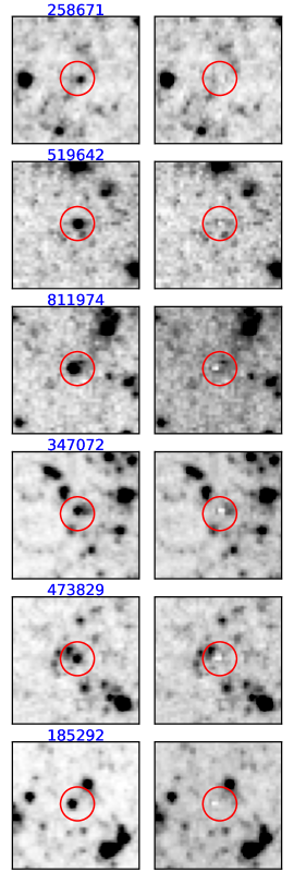
Figure 2: Our PSF photometry for the representative Cepheids in Figure 4 of H16. The left column shows 40$\times$40 pixels in F555W band centered on each Cepheid with the Cepheid ID (which is the same as in H16) given on top of each frame. The right column corresponds to the exact same image with the Cepheid removed after the PSF modeling.

4.1.1 PSF Modelling

To measure the brightness of the Cepheids at each epoch, we use the PSF photometry routines of the Photutils package of Astropy (Bradley et al., 2019) that provides tools similar to, but also more general than, DAOPHOT (Stetson, 1987) which is used by H16. For optical bands, we perform the PSF photometry on 100 pix $\times$ 100 pix (4 by 4 arcsec²) portions of the image centered on each Cepheid for all the epochs. The background is locally estimated for each Cepheid and is automatically subtracted from the Cepheid flux. Similar to H16, we use the TinyTim package that provides PSF models for various cameras and different HST bands (Krist et al., 2011). We checked various fitting algorithms and background estimators and found that the choice has negligible effect on the flux measurement. Therefore, similar to R16, we use a Levenberg–Marquardt-based algorithm (provided by Astropy as LevMarLSQFitter) for determining the best-fit parameters which are the (x,y) position and the flux (plus their uncertainties) for the Cepheids, and MMMBackground routine which calculates the background using the DAOPHOT MMM algorithm (Stetson, 1987).

For IR photometry, i.e. for the F160W band, our procedure is the same as in the optical analysis, except that (similar to R16) the (x,y) positions of the Cepheids are fixed to their best-fit values from the F814W band and that the PSF photometry is performed on 50 pix $\times$ 50 pix (around 6.5 by 6.5 arcsec²) portions of the image centered on each Cepheid. The reason for fixing the (x,y) position is that the significantly lower resolution of IR images may lead the fitting algorithm to pick a wrong neighbouring source rather than the Cepheids if (x,y) are allowed to vary as free parameters.

Examples of our PSF photometry results are shown in Figure 2. We choose to show those Cepheids that are presented as representative by H16 (in their Figure 4).

4.1.2 Epoch-to-epoch offset

The observation condition varies from epoch to epoch and would affect the flux of the Cepheids. To correct for this, we use the local standard stars which were introduced earlier. For each band, we perform a PSF photometry of these non-variable stars and measure their average fluxes in all epochs, $\bar{F}_{\mathrm{all}}$, and also for each epoch, $\bar{F}_{\mathrm{epoch}}$. The Cepheid fluxes at each epoch is then scaled by $\frac{\bar{F}_{\mathrm{all}}}{\bar{F}_{\mathrm{epoch}}}$ to correct for the epoch-to-epoch offset.

4.1.3 Magnitude zero-points and aperture correction

The magnitude zero-point, ZP, for different HST bands are provided by Kalirai et al. (2009), Deustua et al. (2017), and on the STScI calibration pages. These ZP values are based on WFC3 standard aperture radius of 0.4 arcsec. Therefore, the difference between this standard aperture and the PSF modeling should be measured and corrected for. A customary approach adopted also by H16 is to perform both PSF and aperture photometry on a sample of ideally isolated and relatively bright stars in the image and to obtain a statistical mean difference between the two.

In this work, we take a rather different approach. Ideally, for a single isolated star the difference between the aperture and PSF photometry should be directly dependent on the aperture size and the PSF model, while the background should be the same. Here, given that the aperture size for the purpose of correction is fixed to 0.4 arcsec, the difference is basically caused by the extra light captured by the tails of the PSF model beyond 0.4 arcsec radius. Therefore, one way to directly obtain this difference is to measure the flux of the PSF model using a 0.4 arcsec radius aperture (10 pixels for UVIS and around 3 pixels for IR). The magnitude difference, hence the aperture correction ($\mathrm{AP_{cor}}$), would then be

$$\mathrm{AP_{cor}}=2.5\log_{10}[\frac{F_{\mathrm{ap}}}{F_{\mathrm{PSF}}}]-2.5\log_{10}[EE(r=10)],$$ (2)

where $F_{\mathrm{ap}}$ is the fraction of the PSF flux inside the aperture, $F_{\mathrm{PSF}}$ is the total flux of the PSF model, and $EE(r)$ is the encircled energy for different aperture radius $r$ (see Deustua et al., 2017, for further details). We compare the two methods of measuring the aperture correction in Appendix A.

The ZP and $\mathrm{AP_{cor}}$ values used in this study are listed in Table 1 for each band.

	F555W	F814W	F350LP	F160W
ZP (mag)	25.737	24.598	26.708	24.5037
$\mathrm{AP_{cor}}$ (mag)	0.032	0.034	0.032	0.049

Table 1: The zero-point (ZP) and the aperture correction ($\mathrm{AP_{cor}}$) values both in mag for the different HST bands used in this study. See Section 4.1.3.

4.2 Crowding Bias

At distances larger than $\approx 10$ Mpc, despite the large luminosity of Cepheids, their light often cannot be separated from their stellar crowds (Riess et al., 2020). The flux of the neighboring stars entering the same resolution element as the Cepheid alters the statistical estimation of the background, therefore biasing the Cepheid flux (Anderson & Riess, 2018). This bias is one of the most significant challenges for Cepheid measurements at distances larger than 20 Mpc (Freedman et al., 2019). In particular for NGC 5584, at a distance of around 23 Mpc, each pixel of the WFC3/UVIS camera spans around 4 pc. Therefore, it is very likely that the pixel that contains a given Cepheid also encompasses other stellar sources either physically near the Cepheid, or along the line of sight. The pixel size of UVIS/IR is around three times larger than that of WFC3/UVIS, hence covering a larger physical size at the distance mentioned above. The so called ”crowding bias” can be statistically estimated at the location of each Cepheid and can be removed from the flux measurements. A typical method, which is also used by the SH0ES team, is to simulate and add artificial stars to the immediate surroundings of each Cepheid on an image, retrieve their flux using the same PSF photometry approach applied to the Cepheids, and measure the difference between the input and output fluxes. In a recent study, Riess et al. (2020) present a test of this approach using an independent method employing the Cepheids amplitudes, and report an statistical agreement between the two methods.

In this work, we use a similar approach as in R16 and H16. In the case of the optical bands, for each Cepheid we simulate (using TinyTim PSF models) 20 artificial stars per epoch and add them to the same image portions used for their PSF photometry (Section 4.1.1). In the case of the F160W band, because only two epochs are available, we use 50 artificial stars per epoch. The fluxes of these artificial stars are then measured using the same PSF approach explained in Section 4.1.1. Prior to obtaining a mean value for the magnitude differences, H16 directly removes the artificial stars that land within 2.5 pixels of another source that is up to 3.5 mag fainter. Instead of this direct removing approach, we apply a $2\sigma$ clipping which automatically rejects the artificial stars that are blended with another bright source. We then measure the mean magnitude difference as the crowding bias estimate for each Cepheid.

For the optical observations, the SH0ES team uses the mean value of crowding bias in a galaxy as a single bias value for all the Cepheids in that galaxy. By doing that, the local bias are over estimated for some Cepheids, and are underestimated for some others. Crowding is an environment dependent effect and, in principle, it should not be averaged over a galaxy. In our analysis, we take a different but accurate approach and apply the crowding bias estimated at the position of each Cepheid on the measured magnitudes of that Cepheid before template light curve fitting. We investigate the crowding bias in more detail in Appendix B where we derive a relation between crowding bias and local surface brightness and we also compare our results with those of SH0ES.

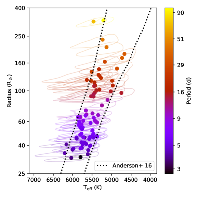
Figure 3: Radius vs. Temperature diagram for the Galactic Cepheids. The dots are the average values (over the pulsation), whereas the thin lines show the values over the pulsation. The color code refers to the pulsation period. The dotted lines are the borders of the theoretical instability strip, using mild rotation (0.5) and solar metallicity (Anderson et al., 2016). We only use the Cepheids with period greater than 12 days for building our template light curves, see Section 4.3.1 for further details.

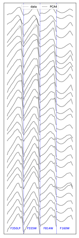
Figure 4: The training set (continuous lines) and reconstructed (doted line) light curves, sorted by pulsation period: from shortest (bottom) to longest (top). See Section 4.3.2.

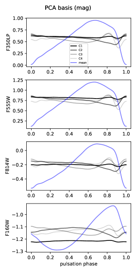
Figure 5: Top four panels: PCA components, in blue the average light curve, and in shades of gray the first 4 components (the darkest is the first component). Bottom: the increase of the training data set variance covered as a function of number of components used in the reconstruction.

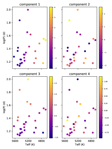
Figure 6: The color coded PCA coefficients as function of Cepheids’ effective temperature and period. Interestingly, component 1 is strongly correlated with temperature, and component 3 is strongly correlated with period.

4.3 Light curve fitting using Templates from Galactic Cepheids

The data collected for each Cepheid consists of several epochs for different pass bands. From this data, we need to derive the pulsation period, as well as the mean magnitudes in each band. In H16, this was done using template light curves from Yoachim et al. (2009). In this work, we use different template light curves and fitting strategy so that all bands are analysed simultaneously.

We derive synthetic light curves in the HST photometric bands for various known Galactic Cepheids, covering the instability strip (in effective temperature and period). The radius, effective temperature, and period of these Cepheids are shown in Figure 3. We then use a dimensionality reduction algorithm to parametrize any light curve using only a few parameters.

4.3.1 Data set for the templates

We choose to use observational data as basis for our templates, fitted with our modeling tool SPIPS (Mérand et al., 2015) which synthesizes photometric observations based on variations of the stellar radius and effective temperature. We collect high quality spectro-, photo- and interferometric data for many Galactic Cepheids and fit their SPIPS models. It should be noted that the knowledge of the distance and/or the projection factor of these Galactic Cepheid does not play a role in building the light curve templates.

Our final sample comprises of 28 stars with periods ranging from 12 to $\sim$90 days (Breuval et al., in prep). We do not include Cepheids with period shorter than 12 days because i) Cepheids observed in distant galaxies are biased towards the brightest ones, which results in an observational cut around $\sim$20 days and ii) Cepheids light curves change dramatically around 9-10 days, which has been long noticed ever since Fourier decomposition was applied to Cepheids’ light curves (see e.g. Simon & Lee, 1981). We do not apply any selection cut on radius and effective temperature, as our intent is to sample Cepheids in the instability strip.

The SPIPS models are based on radial and temperature variations enabling the synthesize of any photometric light curve using the filter band pass definition and atmospheric models. The advantage of this method is that it can accurately extrapolate light curves in pass bands for which we do not have data. We use the HST band passes and zero points defined at the Spanish Virtual Observatory’s Filter Profile Service.

4.3.2 Reduction of dimensions in templates

Our 28 Galactic Cepheids light curves contain a lot of information which needs to be reduced into parametrised templates. We reduce the dimensions of our template data set with a principal component analysis (PCA), using the scikit-learn Python library (Pedregosa et al., 2011). The training data set for PCA are 28 vectors composed of the concatenated light curves (one for each band) over a single pulsation cycle, centered around their means (see Figure 4). When it comes to choosing how many components to keep to fit our light curves, it is customary to consider the amount of variance reproduced by a given number of most significant components. In our dataset, at any given phase and for any bands, the standard deviation is never greater than 0.2 mag, with a total standard deviation of 0.13 mag (around the average light curve). Using enough PCA components to reproduce 95% of the variance should reproduce light curves within $\sim$0.03mag (on average), which we deemed enough for our application. Our main goal is to extract the average magnitude from sparse and irregularly sample time series: even if the light curve is reproduced within 0.03 mag, the average is likely estimated with much higher accuracy. Keeping 3 principal components covers 93.8% of our training set variance, whereas using 4 components leads to 97.1% of the variance being reproduced, which corresponds to a standard deviation of 0.022 mag. See Figures 5, and 6 for different information regarding the PCA components.

4.3.3 Fitting strategy

For a given NGC 5584 Cepheid, we have a list of observations in various pass bands and at different dates. The initial period is estimated by a computed periodogramme on the F555W and F350LP data. Then, a full model is fitted to the data using the PCA light curves. Our model also includes reddening, using the formula contained in SPIPS and parametrised using the color excess E(B-V). We fix the reddening to E(B-V)=0.035, which we estimate using DUST

We iterate on the initial parameter by randomising the period ($\pm$5%) to account for the uncertainty of the periodogramme estimation. The PCA coefficients are initialised to their mean value from the analysis of the template stars. During the least square fit, a uniform prior constrains the coefficient to only evolve inside the range of values observed on the template stars. From the randomised starting periods, we keep the fit with the global lowest reduced $\chi^{2}$. Using the best fit parameters and covariance matrix, we can compute the domain of uncertainty for the synthetic light curves and derive the average magnitudes and amplitudes.

Our fitting method has several differences with the one presented in H16 using Yoachim et al. (2009). First of all, we fit all data at once. This is feasible since our model include realistic information about the offset between bands and the shape of the light curve. An example can be seen for star 347072 in Figure 7 (which we discuss further in Section 5). The F814W data of this Cepheid are very noisy and the fitted light curve is constrained mostly by the F555W and F350LP data, which are of much better quality. Even if the modeled light curve in F814W is systematically above the data points, it is the most realistic within our hypothesis and priors derived from Galactic Cepheids.

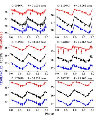
Figure 7: Our light curves of the Cepheids presented by H16 as representative Cepheids (see their Figure 4). On each panel, the bottom (blue), middle (black), and top (red) curves are light curves in F350LP, F555W, and F814W, respectively. Two cycles are plotted and F350LP and F814W have 1.25 and 0.25 mag offsets, respectively. The shaded transparent regions represent the model uncertainties and are present for every curve on all panels. For some curves, they are too small to be seen by eye.

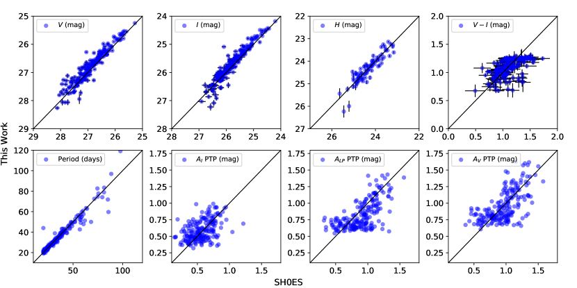
Figure 8: Comparing our results (Y axes) with those the SH0ES (X axes) team for mean magnitudes (LP: F350LP, V: F555W, I: F814W, H:F160W), $V-I$ color, period, and light curve amplitudes ($A$) of the Cepheids in NGC 5584. For the H band, we only show the uncertainties on the Y axis (i.e. from our results), since R16 publishes only the so called total uncertainties ($\sigma_{tot}$) and not those of the mean magnitudes in the $H$ band. PTP stands for peak-to-peak and is one of the methods of determining the pulsation amplitudes (see Section 5.2 for more details). The equality lines are plotted with solid black on all panels.

5 Results

5.1 Light Curves, Mean Magnitudes, and Periods

Using the light curve template fitting explained in Section 4.3, we obtain the periods and the mean magnitudes for all the identified Cepheids in the four HST bands. Figure 7 presents our results for the light curves of the Cepheids we showed in Figure 2, they are chosen by H16 as the representative Cepheids of NGC 5584. Our light curves can be directly compared with those of H16 shown in their Figure 4. Most of the light curve models nicely represent the data. One exception among these is the Cepheid 347072, which as discussed earlier, has poor quality data points in F814W. This Cepheid is not detected in the F160W band and therefore is not included in the measurement of distance neither by SH0ES nor by us in this work.

Figure 8 provides one-on-one comparisons of our results with those of SH0ES reported in H16 and R16. The top row provides comparisons for the mean magnitude measurements in $V$, $I$, and $H$ bands, as well as the $(V-I)$ color. For the H band, we only show the uncertainties on the Y axis (i.e. from our results), since R16 publishes only the so called total uncertainties ($\sigma_{tot}$) and not those of the mean magnitudes in the $H$ band. A generally good agreement can be seen between the two results, especially for the H band and the $V-I$ color both of which directly contribute to the distance measurement (see Equation 1).

The left-most panel on the bottom row of Figure 8 provides a comparison for period measurements. As can be seen, although we use a different approach for template fitting and hence the period measurements, the two results are in general agreement with only a few exceptions.

Regrettably, H16 does not provide mean magnitudes in F350LP band, we therefore cannot have a direct comparison for this quantity. However, we can compare amplitude measurements in F350LP band as discussed in the next sub-section.

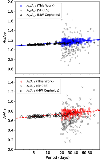
Figure 9: RMS (root-mean-square) amplitudes in V (top panel) and I (bottom panel) bands relative to F350LP (LP) band vs. period. The plus and cross symbols are SH0ES results for $A_{V}/A_{LP}$ and $A_{I}/A_{LP}$, respectively. Our results have a significantly lower scatter than those of SH0ES. The solid blue and red dashed lines are linear fits as explained in Section 5.2 and shown in Equation 3. We also show the MW Cepheids as filled dots and empty circles, for $A_{V}/A_{LP}$ and $A_{I}/A_{LP}$, respectively. We note that while for the linear fitting only the results from the Cepheids in NGC 5584 were used, and while only 28 of the MW Cepheids with period$>$12 days were used for our template light curve building, the fitted line passes also through the Milky Way Cepheids data points.

5.2 Amplitude Measurements

We remind the reader that H16 uses the amplitude ratios vs. period relation of the Cepheids in NGC 5584 to correct the random-phase observations of other SNIa host galaxies in the $V$ and $I$ band. Therefore, an accurate and precise measurement of these relations can potentially impact the final $H_{0}$ measurements. The three panels (from the right) on the bottom row of Figure 8 provide comparisons for our amplitude measurements vs. those of the SH0ES team. We perform two different measurements of the amplitudes: 1) peak-to-peak (PTP) which measures the magnitude difference between the maximum and minimum of the light curve model, and 2) the root-mean-square (RMS) which is the standard deviation of the light curve (regularly sampled) from their mean value. While the PTP results (which are the ones shown in Figure 8) are in general agreement with the amplitude measurements of SH0ES, it is not robustly estimated in our method. Our PCA-based fits allow variations in the shape of the model, especially between phase 0.8 an 1.0, which is where the amplitude is measured (see for example F350LP light curve of star 258671 in Figure 7). On the other hand, the amplitude is directly one of the template fitting parameter in the SH0ES analysis. While PTP and RMS differ by a factor of $2\sqrt{2}\approx 2.83$ for a pure sinusoidal wave, the value varies with the exact shape of the light curve. From our high definition template sample star, we find that $\left(\frac{\mathrm{PTP}}{\mathrm{RMS}}\right)_{I}=3.08\pm 0.12$ and $\left(\frac{\mathrm{PTP}}{\mathrm{RMS}}\right)_{V}=3.14\pm 0.14$. We are interested in ratios between bands, and the comparison with SH0ES’ results. For the amplitude ratios we find that $\left(\frac{\mathrm{PTP}_{I}}{\mathrm{PTP}_{V}}\right)=0.98\pm 0.03\left(\frac{\mathrm{RMS}_{I}}{\mathrm{RMS}_{V}}\right)$. In other words, the ratio of amplitudes are almost independent of the amplitude measurement method and our amplitude ratios computed from RMS (which we use in our subsequent analysis) are comparable to those of SH0ES with a scatter of 6%.

In Figure 9, we compare our results and those of SH0ES for the amplitude ratio vs. period relation. The blue squares and red diamonds are our $A_{V}/A_{LP}$ and $A_{I}/A_{LP}$, respectively. The grey plus and cross symbols are the same quantities as published by SH0ES in H16 and have significantly larger scatters. The dots and empty circles are, respectively, $A_{V}/A_{LP}$ and $A_{I}/A_{LP}$ for the Milky Way Cepheids. The blue solid line, and the red dashed line are our results of linear fits on $A_{V}/A_{LP}$ and $A_{I}/A_{LP}$ vs. $\log P$. While for the linear fitting we only used the data from the Cepheids in NGC 5584, and while only 28 of the MW Cepheids with period$>$12 days were used for our template light curve building, the fitted line passes also through the Milky Way Cepheids data points even for those with small periods. The linear correlation coefficient measured for both of these relations are $\approx 0.3$. From the linear fitting we find

$$\begin{split}&A_{V}/A_{LP}=1.167+0.073(\log P-1.5),\>\sigma_{fit}=0.014,\\ &A_{I}/A_{LP}=0.757+0.090(\log P-1.5),\>\sigma_{fit}=0.022,\end{split}$$ (3)

where $\sigma_{fit}$ values are the standard deviations of the fits and are an order of magnitude smaller than those of SH0ES (see Table 2 of H16). The small scatter in this relation means that our amplitude ratio measurement is less noisy and is indicative of a high quality light curve modelling approach. We note that in H16 the light curves of different bands are fitted separately (using Yoachim et al. (2009) templates), and then the amplitudes resulting from the different fits are divided to yield the amplitude ratios. This could be the reason for the large scatter in their amplitude ratios. On the other hand, in our approach, all the light curves (of all bands) are fitted simultaneously, hence the amplitudes are not estimated independently from one another, leading to a lower scatter.

5.3 Uncertainties on the Wesenheit H Magnitudes

In their section 2.2, R16 describe a $\sigma_{tot}$ as the total uncertainty on their Cepheid distance measurements. They refer to the uncertainty of the crowding bias in the H band as $\sigma_{sky}$ and that of the optical observations as $\sigma_{ct}$ and they add them as a single value for all the Cepheids in a given galaxy. Since we apply the crowding bias (in all bands) for each Cepheid before the template fitting, the values of mean magnitudes already include the effect of crowding bias and their uncertainties. In addition, our template light curve fitting method analyses all the data together, therefore, the uncertainty on the H band mean magnitudes, already includes the effect of limited phase coverage.

Therefore, for the total uncertainty on $W_{H}$ we have

$$\sigma_{WH}=[\sigma^{2}_{H}+R_{H}^{2}(\sigma_{V}^{2}+\sigma_{I}^{2})+\sigma^{2}_{int}]^{1/2},$$ (4)

where $\sigma_{int}$ is the intrinsic dispersion due to the nonzero width of the instability strip. To estimate $\sigma_{int}$, we follow the procedure of Riess et al. (2019). Using the Cepheid observations in the LMC, Riess et al. (2019) present PL relations and their scatter in different HST bands. To estimate $\sigma_{int}$, they subtract (in quadrature) the mean Cepheid measurement errors from the scatter of the PL relation for a given band. Their mean measurement error for different bands are given in their section 2.2 and the values for the scatter of the PL relations are listed in their Table 3. For $W_{H}$, the intrinsic dispersion is estimated to be $\sigma_{int}=0.069$ mag.

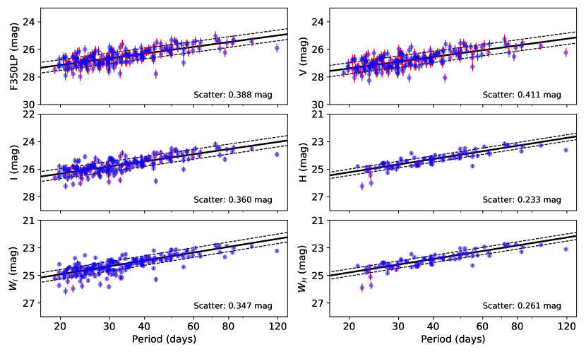
Figure 10: Period-Luminosity relations in the four HST bands and also for the $W_{I}$ and $W_{H}$ Wesenheit indices. The uncertainties on individual Cepheids in this figure also includes the contribution from the $\sigma_{int}$ explained in Section 5.3. The solid lines represent the results of fitting a linear relation of the form $m=\alpha\log P+\beta$ with a $3\sigma$ clipping. The slopes ($\alpha)$ are fixed to the values for LMC Cepheids given in Table 3 of Riess et al. (2019), see Section 5.4.

5.4 The Period-Luminosity Relations

In addition to the PL relation in $W_{H}$, we also present PL relations for all the bands F350LP, F555W, F814W, F160W, as well as for optical Wesenheit index, $W_{I}$ in Figure 10. The latter is defined as $W_{I}=I-R_{I}(V-I)$ with $R_{I}=1.3$ (Riess et al., 2019). The uncertainties on individual Cepheids in this figure also includes the contribution from the $\sigma_{int}$ explained in the previous section. We note that the data points in the PL relations shown in Figure 6 of H16 appear to contain only the measurement uncertainties which are comparable in size to this work’s results as shown in our Figure 8.

The solid lines represent the results of fitting a linear relation of the form $m=\alpha\log P+\beta$, where $m$ is the mean magnitude. We fix the slope $\alpha$ to the values given in Table 3 of Riess et al. (2019) (which lists the PL relations from Soszynski et al. (2008), Macri et al. (2015), and R16), and fit for the intercept with a $3\sigma$ clipping. The slightly larger scatter in our PL relations compared to those found by SH0ES for NGC 5584 is most probably due to our different treatment of the crowding bias. As stated earlier in the text, SH0ES add a single value of crowding bias for all the Cepheids in a galaxy which shifts the PL relation slightly towards fainter values. However, we add the crowding bias values estimated at the location of each Cepheid separately which introduces a somewhat larger scatter in the PL relation.

5.5 The Distance to NGC 5584

In this section, we derive the distance modulus of NGC 5584, based on apparent Wesenheit magnitudes $W_{H}$ of our sample of 82 Cepheids in this galaxy. By applying an existing $W_{H}$ PL relation to the known period of our stars, we derive the absolute magnitude $M^{W}_{H}$ for each Cepheid and then their individual distance modulus $\mu=W_{H}-M^{W}_{H}$.

We perform this calculation using two different PL relations: one calibrated in the Milky Way (Breuval et al., 2020), $M^{W}_{H}=-5.432\>(\pm 0.029)-3.332\>(\pm 0.177)[\log P-0.84]$, and another calibration from the LMC (Riess et al., 2019), $M^{W}_{H}=15.898-3.26\log P$. For the slope of the latter relation, a 0.02 mag uncertainty is stated in Riess et al. (2019) while they mention no uncertainty on the intercept. Therefore, we assume a conservative uncertainty of 0.02 mag error also for the intercept (the intercept uncertainties in Macri et al. (2015) are much smaller than 0.02 mag). We then subtract the LMC distance modulus as measured by Pietrzyński et al. (2019). For both PL relations, the individual distance moduli obtained for each Cepheid are represented in Figure 11. The Galactic PL relation yields a weighted mean distance modulus of $31.810\pm 0.047$ mag, while the LMC calibration results in $31.639\pm 0.038$ mag. The $1\sigma$ confidence regions of these weighted mean values are also shown in Figure 11. The distance modulus from the Galactic PL relation is in agreement with $\mu=31.786\pm 0.046$ (mag) measured by SH0ES in R16. The distance modulus from the LMC PL relation, however, is smaller though still in agreement within $2.5\sigma$ with SH0ES result.

It is not surprising to obtain different distances based on LMC and MW PL relations, given that LMC has a smaller metallicity compared to the MW (Romaniello et al., 2008), i.e. the larger distance inferred from LMC PL relation is consistent with its smaller metallicity. The difference in terms of distance modulus obtained with MW and LMC PL relations highlights the need for a metallicity correction which has been extensively studied (see e.g. Pietrzyński et al., 2004; Gieren et al., 2018; Groenewegen, 2018; Ripepi et al., 2019, 2020, and Breuval et al. 2021, in prep.), though yet with no clear consensus. However, NGC 5584 is a spiral galaxy with a structure similar to that of MW and, in fact, its metallicity gradient is very similar to that of the MW (see table 6 of Balser et al., 2011, and table 8 of R16). The MW PL relation, therefore, is more appropriate for measuring the distance to NGC 5584.

From our $\mu$ for NGC 5584 based on MW PL relation, we calculate a distance of $d_{\mathrm{NGC~{}5584}}=23.01\pm 0.05$ Mpc.

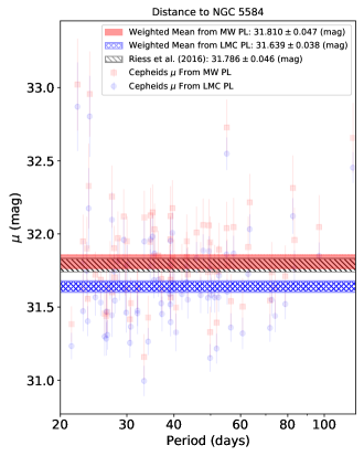
Figure 11: Distance modulus $\mu$ measured from $W_{H}$ vs. period for Cepheids in NGC 5584 using two PL relations from MW (red squares) and LMC (blue circles) Cepheids. The horizontal filled rectangles show the $1\sigma$ confidence regions for measured distances. The uniformly red and the blue crossed-diagonal hatched regions represent our measurements based on the MW and LMC PL relations, respectively, and are the weighted means of the $\mu$ values measured for individual identified Cepheids. The black back-diagonal hatched region represent the estimated distance reported by R16.

6 Conclusion

The $4-6\sigma$ tension (Riess, 2019) between the direct and the early Universe measurements of $H_{0}$ asks for detailed investigations in the different methods involved. NGC 5584 played a key role in the direct measurement of $H_{0}$ from the Cepheid distance ladder by the SH0ES team (Riess et al., 2016). Observations of this galaxy was employed to derive a relation between the ratio of pulsation amplitude of Cepheids in $V$ and $I$ bands relative to the wide F350LP HST band and the period. The F350LP band has been used by the SH0ES team for detection and light curve measurement of Cepheids in around half of the current SNIa host galaxies used for $H_{0}$ measurements and the relation mentioned above has been used to obtain mean $V$ and $I$ magnitudes from the spars sampling of Cepheid light curves in these bands.

In this contribution, we provided an independent and detailed analysis of the HST data from NGC 5584. Where possible, we intentionally used methods and tools different from those used by SH0ES. This allowed the investigation of possible influence of these methods on distance measurements. The key parts of our detailed analysis can be listed as follows:

• applying PSF photometry routines of Photutils package of Astropy (Bradley et al., 2019), instead of the classic DAOPHOT software (Stetson, 1987),

• testing and finding negligible influence of the choice of PSF modelling and background subtraction algorithms,

• applying a different aperture correction procedure for the PSF photometry,

• adopting a slightly modified approach for crowding bias estimation (using a sigma-clipping approach on the artificial stars flux measurement rather than directly removing bright estimated sources done by SH0ES),

• a different approach for applying the crowding bias compared to SH0ES (applying the bias separately for each Cepheid rather than averaging over the whole galaxy for the optical observations), and

• employing a completely different approach for Cepheid light curve modelling for measurement of mean magnitudes, amplitudes, and periods.

And our main results can be summarised as follows:

• Our measurements of Cepheids’ mean magnitudes and period and those of SH0ES are in good agreement. In particular, we find no systematic difference in our H band mean magnitudes and (V-I) color, both of which directly influence the distance measurements, compared to SH0ES.

• We derived a significantly tighter amplitude ratio vs. period relation compared to the one derived by SH0ES.

• We measure two distance moduli for NGC 5584 using two different PL relations calibrated in MW and LMC. The result from the former is in agreement with the value from SHOES within $1\sigma$, and the result from the latter is $0.147\pm 0.060$ mag smaller than that of SH0ES, though still within $2.5\sigma$.

We do not attempt at reporting a value for $H_{0}$ based on the distance to only one SNIa host galaxy, and we only note that a smaller distance to NGC 5584 points towards a higher $H_{0}$ value. However, we consider the MW PL relation to be more appropriate for distance measurements to NGC 5584, due to similar metallicity and structure of these two galaxies. Nevertheless, the effect of metallicity and its measurement methods (Bresolin et al., 2009; Kudritzki et al., 2012) on extragalactic Cepheid distances requires further investigations.

The main conclusion of the current study is that our inspection of NGC 5584 Cepheids does not yield any systematic hints towards the resolution of the $H_{0}$ problem. However, it would be important to also independently inspect for systematics in the distance measurements to all the galaxies used for calibration of SNeIa absolute magnitude. For doing so, and until reasonably fine-sampled time series data of all SNeIa calibrators become available, it would certainly be better to use our precise amplitude ratio vs. period relations for light curve analysis of Cepheids in SNeIa hosts with limited time series data as they would potentially yield more accurate mean magnitudes in V and I bands. This would also provide an investigation into the potential statistical effect of these relations in $H_{0}$ measurements.

While it is important to continue the investigations on the $H_{0}$ measurements, the current findings seems to be pointing towards a non-trivial solution to this problem. This could mean that our current understanding of the local or early Universe may require modifications or a complete change of paradigm. In the local Universe, presence of a large local underdensity (which is incompatible with LCDM, Haslbauer et al., 2020) has been presented (Shanks et al., 2019; Haslbauer et al., 2020) as a possible cause of the $H_{0}$ discrepancy (but see also Riess et al. 2018a and Shanks et al. 2018). In the early Universe, various scenarios such as non-standard recombination, dark matter/dark energy interaction, and self-interacting neutrinos have been presented, however, so far no consensus has been reached (for reviews and summaries see Verde et al., 2019; Poulin, 2020; Knox, 2020).

While it is important to seek alternative ideas on the theoretical side, the improvement of current observational methods as well as the development of new independent ones are necessary for a progress towards a solution to the $H_{0}$ problem. For the Cepheid distance ladder, the number of SNeIa calibrators observed by the HST is soon to be doubled by the SH0ES program (Riess et al., 2019), hence the statistical uncertainty on $H_{0}$ measured by this method would be reduced. In addition to strong lensing, megamasers, and TRGB methods (see also Beaton et al., 2016; Kim et al., 2020) mentioned in the Introduction, other Cepheid-independent routes would also soon contribute to $H_{0}$ measurements. Huang et al. (2020) presents Mira variables for calibration of SNeIa absolute magnitudes. Also, using the advanced LIGO and Virgo gravitational wave detectors, The LIGO & Virgo Collaborations et al. (2019) have reported an $H_{0}$ measurement using standard sirens (see also Coughlin et al., 2020). As the number of detected standard sirens increases in future, the currently large statistical uncertainty in their resulting $H_{0}$ measurement would decrease, making them an important independent way of measuring the cosmic expansion rate (Feeney et al., 2019).

One of the most promising contributions to the accuracy of the cosmic distance scale in the near future would be from Gaia. The impact of the first (see, e.g., Casertano et al., 2017; Gaia Collaboration et al., 2017) and second (see, e.g., Groenewegen, 2018; Riess et al., 2018b; Clementini et al., 2019; Breuval et al., 2020; Ripepi et al., 2020) data releases of Gaia on the calibration of the Cepheid PL relation is already considerable. It is however still limited by the persistently uncertain value of the instrumental parallax zero point (see, e.g., Arenou et al., 2018; Khan et al., 2019). The early Gaia data release 3 (EDR3) published on 4 December 2020 (Gaia Collaboration et al., 2020) significantly improved the accuracy of the measured MW Cepheid parallaxes of MW Cepheids. A mitigation of the uncertainty due to the instrumental parallax zero point through an ad hoc position-, color- and magnitude- dependent calibration is also presented by Lindegren et al. (2020). As discussed by Riess et al. (2021) (see also Breuval et al. 2021, in prep.), this improvement brings the calibration of Cepheids luminosities to a 1% level, which makes them the most accurate distance indicators available to date. As the number of measurement epochs and the understanding of the Gaia instrument increase, the DR3 and DR4 will eventually provide trigonometric reliable parallax measurements at a few percent level or better for hundreds of Milky Way Cepheids. Combined with accurate photometry and extinction corrections from 3D extinction maps (see, e.g., Chen et al., 2019; Hottier et al., 2020), this set of absolutely calibrated distances will result in a very tight set of Cepheid PL relations, calibrated for the solar metallicity. Our Galaxy therefore appears as a particularly appealing alternative to the Magellanic Clouds as the primary anchor for extragalactic Cepheid distances, thanks to the similarity of its metallicity with those of distant SNeIa host galaxies. Relying on Milky Way Cepheids presents the advantage of reducing the possible bias introduced by the metallicity correction. This will effectively bypass the metallicity correction, thus increasing the overall robustness of the SNeIa calibration.

As also noted in Riess (2019), precise measurement of $H_{0}$ provides a powerful end-to-end test of the LCDM standard model of cosmology. Future observational progress and inspections such as the current study would eventually conclude whether the $H_{0}$ tension is caused by a measurement error, or it means that the LCDM should be abandoned as a correct model of the Universe.

Appendix A Aperture Correction

Here, we compare aperture correction using the aperture photometry of the PSF model with the approach using aperture and PSF photometry of stars in the image. For this purpose we compare the PSF and aperture photometry of thirteen uncrowded stars using the stacked version of all the F555W band images. For these stars we crop a 50 pixel $\times$ 50 pixel portion of the image and perform the PSF photometry in the same way as described in Section 4.1.1. All the sources except from the central star are removed using the PSF modelling prior to the aperture photometry with an aperture radius of 10 pixels. The difference is then measured using Equation 2 and we find a mean value of $AP_{cor}=0.056\pm 0.024$ mag for the F555W band. It is $1\sigma$ larger than the value obtained using aperture photometry of the PSF model. We expect a similar result for F814W band. For the F160W band, the $AP_{cor}$ we measure using the PSF model, i.e. 0.049 mag, is also around $1\sigma$ smaller than the $0.06\pm 0.01$ measured by Huang et al. (2020) for F160W images of the SNIa host NGC 1559. The difference of these two methods is most probably due to imperfect subtraction of the background noise in the actual images and the absence of this noise in the PSF model. Therefore, by noting that the difference in the F160W band is most relevant for distance measurement (Equation 1), measuring $AP_{cor}$ using aperture photometry of the PSF model rather than using uncrowded stars in the image leads to around $0.01\pm 0.01$ mag decrease in the distance modulus.

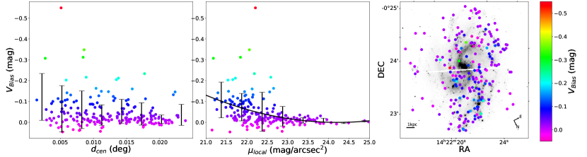
Figure 12: Left: V band crowding bias ($V_{Bias}$) vs. the projected angular distance $d_{cen}$ in degrees from the center of the galaxy. Middle: $V_{Bias}$ vs. local surface brightness $\mu_{local}$. Right: Distribution of the Cepheids in the NGC 5584 with the color code being the estimated crowding bias at the position of each Cepheid in the V band. The same color code is also used in the other panels. The Cepheids that are most affected by the crowding bias are statistically closer to the centre of the galaxy, however, the bias is found to be more correlated with local surface brightness. The linear correlation coefficient between the absolute value of the crowding bias and $d_{cen}$ and $\mu_{local}$ are $r=-0.24$ and $r=-0.40$, respectively. See appendix B for details.

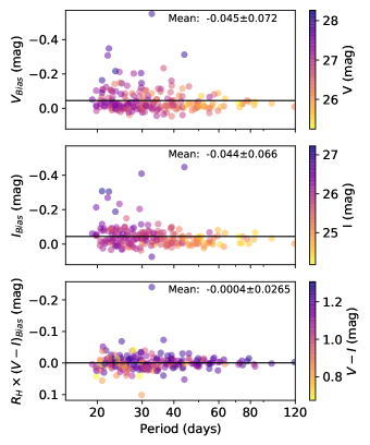
Figure 13: Crowding bias in V and I bands, as well as $R_{H}(V-I)$ vs. period. This figure can be directly compared to Figure 14 of H16 (see appendix B for a discussion).

Appendix B Crowding Bias

In Section 4.2 we explained our method of estimating the crowding bias at the location of each Cepheid. Here we investigate the environmental dependence of crowding bias in the F555W band. Figure 12 shows the distribution of crowding bias across the galaxy (right panel), bias vs. the projected angular distance $d_{cen}$ in degrees from the center of the galaxy (left panel), and bias vs. local surface brightness, $\mu_{local}$ (middle panel). The Cepheids that are most affected by the crowding bias are statistically closer to the centre of the galaxy where the stellar density is generally higher. However, small bias values can also be found at smaller $d_{cen}$ and we measure a correlation coefficient of $r=-0.24$ between the absolute value of the crowding bias and $d_{cen}$. The small correlation is possibly due to spiral structure of NGC 5584, i.e. even at small galactocentric distances, there are less crowded regions.

We also check the crowding bias vs. $\mu_{local}$. The latter is measured using the following three step method: i) we first measure the average sky background using around twenty 40$\times$40 pixel square regions outside the parts of the image covered by NGC 5584, ii) we then used the same size squares at the location of each Cepheid (where we already estimated crowding bias) and measured the total flux inside them, iii) in the end, the average sky background is subtracted from the local total fluxes and the result is converted to surface brightness using the angular area in arcsec and the magnitude zero point. We measure a correlation coefficient of $r=-0.40$ between the crowding bias and $\mu_{local}$. This relatively larger correlation implies that the local surface brightness is a better proxy to crowding bias compared to galactocentric distance. Using a second order polynomial fit we find

$$\mathrm{Bias}=-0.013\mu_{local}^{2}+0.61\mu_{local}-7.4$$ (B1)

with the standard deviation of the model minus data being $\sigma_{fit}=0.066$. This relation may be used to estimate the crowding bias in the F555W band from the local surface brightness instead of the artificial star injection approach. It may be useful to note that in the regions with $\mu_{local}\gtrsim 23$ mag/arcsec², the effect of crowding bias is negligible.

To compare our crowding bias measurements with those of H16, we also show the bias as a function of period in Figure 13. This figure can be directly compared to Figure 14 of H16. Our results is (within $1\sigma$) in agreement with those of the H16. In particular, as can be seen in the lowest panel, the effect of the crowding bias on the V-I color measurement is very small. We remind the reader that unlike the approach of SH0ES (averaging over the galaxy for the optical observations), we apply the crowding bias estimated for individual Cepheids on their photometric results before the template fitting.

Appendix C Cepheid Properties

Our results for the photometric properties of the identified Cepheids in NGC 5584 are listed in Table 2.

Table 2: Our measurements for the photometric properties of the Cepheids in the NGC 5584.

ID	RAJ2000	DECJ2000	LP	$\sigma_{LP}$	$A_{LP}$	$V$	$\sigma_{V}$	$A_{V}$	$I$	$\sigma_{I}$	$A_{I}$	$H$	$\sigma_{H}$
	(deg)	(deg)	(mag)	(mag)	(mag)	(mag)	(mag)	(mag)	(mag)	(mag)	(mag)	(mag)	(mag)
82928	215.5872	-0.3685	26.717	0.019	0.313	26.943	0.024	0.36	25.899	0.044	0.231	24.859	0.1
86318	215.5892	-0.3676	26.985	0.023	0.274	27.286	0.025	0.326	26.04	0.024	0.22	-	-
91999	215.5886	-0.3682	27.392	0.047	0.306	27.696	0.046	0.361	26.442	0.05	0.243	-	-
96368	215.584	-0.3708	26.841	0.018	0.214	27.11	0.023	0.255	25.945	0.039	0.17	-	-
97566	215.5886	-0.3685	26.3	0.019	0.203	26.6	0.02	0.244	25.35	0.019	0.166	24.107	0.023
111577	215.5875	-0.3698	25.58	0.008	0.18	25.793	0.012	0.21	24.773	0.017	0.133	23.775	0.042
121760	215.588	-0.3701	27.399	0.059	0.29	27.701	0.07	0.343	26.453	0.107	0.231	-	-
134935	215.5855	-0.372	25.963	0.011	0.232	26.213	0.015	0.272	25.099	0.02	0.179	-	-
143986	215.5898	-0.3703	25.809	0.019	0.168	25.984	0.028	0.192	25.067	0.026	0.116	24.187	0.065
151156	215.5928	-0.3691	27.043	0.055	0.186	27.282	0.074	0.22	26.193	0.07	0.143	-	-
156158	215.5903	-0.3706	26.541	0.019	0.245	26.715	0.026	0.277	25.808	0.031	0.171	-	-
157119	215.5914	-0.3701	25.616	0.016	0.234	25.824	0.019	0.269	24.823	0.027	0.171	23.838	0.059
172880	215.589	-0.3721	25.385	0.036	0.172	25.673	0.04	0.205	24.444	0.039	0.128	23.24	0.062
175404	215.591	-0.3712	26.232	0.018	0.182	26.528	0.019	0.221	25.284	0.016	0.149	-	-
175413	215.5939	-0.3697	26.399	0.02	0.206	26.69	0.026	0.25	25.463	0.026	0.169	24.233	0.061
185292	215.5952	-0.3696	25.475	0.008	0.211	25.635	0.012	0.237	24.761	0.009	0.144	23.914	0.025
191706	215.5961	-0.3695	26.359	0.017	0.17	26.569	0.023	0.198	25.558	0.029	0.124	24.575	0.067
197260	215.59	-0.3729	27.219	0.03	0.26	27.521	0.03	0.308	26.268	0.031	0.208	-	-
200467	215.5944	-0.3707	26.947	0.033	0.285	27.253	0.033	0.338	25.992	0.034	0.227	24.72	0.045
200686	215.5899	-0.3731	25.929	0.022	0.186	26.234	0.024	0.229	24.97	0.024	0.157	-	-
208725	215.5952	-0.3708	26.322	0.016	0.266	26.524	0.021	0.304	25.543	0.027	0.193	-	-
211148	215.5834	-0.3769	27.295	0.035	0.299	27.546	0.043	0.347	26.435	0.076	0.226	-	-
216328	215.5967	-0.3704	26.468	0.037	0.21	26.767	0.038	0.255	25.52	0.038	0.176	-	-
220248	215.5879	-0.3751	26.293	0.016	0.294	26.526	0.021	0.339	25.462	0.023	0.219	24.399	0.051
229600	215.5929	-0.373	26.922	0.027	0.252	27.162	0.032	0.293	26.076	0.041	0.191	-	-
230093	215.5895	-0.3747	26.99	0.017	0.207	27.263	0.021	0.248	26.085	0.029	0.165	24.914	0.067
238461	215.5937	-0.373	26.733	0.022	0.268	27.037	0.023	0.319	25.781	0.021	0.216	24.51	0.023
247527	215.5757	-0.3826	26.551	0.019	0.296	26.801	0.024	0.343	25.691	0.037	0.225	-	-
253461	215.5963	-0.3724	26.342	0.018	0.193	26.636	0.018	0.235	25.4	0.019	0.16	24.163	0.024
254240	215.6057	-0.3677	26.154	0.013	0.319	26.418	0.016	0.371	25.27	0.023	0.243	-	-
258671	215.5955	-0.3731	27.075	0.04	0.223	27.349	0.051	0.266	26.172	0.081	0.179	-	-
267902	215.5968	-0.373	25.861	0.014	0.227	26.066	0.02	0.261	25.072	0.021	0.166	-	-
271193	215.5966	-0.3732	26.321	0.019	0.171	26.569	0.028	0.204	25.456	0.029	0.133	-	-
271677	215.5882	-0.3775	27.113	0.024	0.23	27.413	0.024	0.277	26.166	0.025	0.188	-	-
276835	215.5827	-0.3806	26.582	0.036	0.243	26.696	0.047	0.266	25.948	0.068	0.157	-	-
281768	215.5913	-0.3764	27.006	0.02	0.284	27.277	0.028	0.331	26.111	0.039	0.219	24.945	0.092
290494	215.6083	-0.3682	26.103	0.012	0.267	26.304	0.015	0.305	25.322	0.025	0.195	-	-
295981	215.5898	-0.3779	25.913	0.013	0.193	26.104	0.016	0.221	25.145	0.027	0.138	24.21	0.062
298430	215.6007	-0.3724	26.845	0.024	0.41	27.071	0.03	0.469	26.031	0.047	0.302	24.993	0.107
321323	215.5979	-0.375	26.971	0.038	0.218	27.269	0.037	0.262	26.027	0.041	0.178	-	-
321793	215.5995	-0.3742	26.995	0.031	0.196	27.164	0.038	0.221	26.266	0.062	0.135	-	-
325206	215.5894	-0.3795	25.933	0.018	0.207	26.226	0.024	0.25	24.994	0.029	0.17	23.76	0.069
325458	215.5992	-0.3745	27.414	0.102	0.286	27.723	0.103	0.338	26.453	0.102	0.228	-	-
325693	215.5909	-0.3788	27.443	0.056	0.264	27.636	0.074	0.3	26.678	0.113	0.191	-	-
325718	215.5996	-0.3744	25.435	0.011	0.178	25.726	0.011	0.215	24.492	0.011	0.14	23.272	0.013
326705	215.5967	-0.3759	27.603	0.037	0.443	27.754	0.046	0.5	26.917	0.075	0.312	-	-
329366	215.6014	-0.3736	26.959	0.028	0.193	27.255	0.029	0.235	26.012	0.03	0.159	24.771	0.039
330805	215.599	-0.3749	26.173	0.015	0.183	26.361	0.02	0.21	25.411	0.021	0.13	-	-
339133	215.5806	-0.3847	25.609	0.009	0.185	25.813	0.013	0.213	24.817	0.014	0.135	-	-
340379	215.5949	-0.3775	26.966	0.055	0.203	27.119	0.076	0.227	26.263	0.1	0.137	25.44	0.237
342112	215.5925	-0.3788	26.002	0.015	0.175	26.278	0.019	0.212	25.09	0.025	0.141	-	-
347072	215.5997	-0.3754	25.593	0.018	0.164	25.803	0.02	0.191	24.791	0.044	0.12	-	-
353561	215.594	-0.3786	26.399	0.046	0.164	26.642	0.064	0.195	25.54	0.096	0.126	-	-
354807	215.594	-0.3787	25.535	0.018	0.159	25.757	0.026	0.184	24.707	0.026	0.111	23.699	0.064
374736	215.5992	-0.377	26.048	0.013	0.242	26.286	0.015	0.281	25.205	0.024	0.183	24.136	0.055
378235	215.6091	-0.3721	26.737	0.016	0.264	26.989	0.022	0.308	25.873	0.028	0.201	24.76	0.065
390652	215.6005	-0.3771	26.415	0.021	0.239	26.603	0.026	0.272	25.656	0.037	0.17	24.731	0.084
395114	215.5969	-0.3792	25.537	0.017	0.184	25.853	0.019	0.228	24.557	0.022	0.157	23.258	0.04
396420	215.6059	-0.3747	26.928	0.018	0.213	27.224	0.018	0.258	25.984	0.019	0.177	-	-
399436	215.5982	-0.3788	26.727	0.029	0.332	26.893	0.04	0.375	26.011	0.044	0.233	-	-
411135	215.597	-0.3799	25.921	0.012	0.281	26.153	0.017	0.325	25.091	0.025	0.21	24.039	0.062
412396	215.6	-0.3785	26.137	0.023	0.192	26.308	0.033	0.218	25.403	0.044	0.133	24.528	0.105
418643	215.5894	-0.3842	26.447	0.016	0.3	26.743	0.023	0.353	25.511	0.03	0.236	-	-
419182	215.5993	-0.3792	26.311	0.023	0.196	26.476	0.027	0.221	25.587	0.048	0.134	-	-
420418	215.5948	-0.3815	26.579	0.026	0.219	26.83	0.035	0.258	25.712	0.037	0.17	-	-
421192	215.5971	-0.3804	26.244	0.009	0.362	26.511	0.012	0.419	25.36	0.017	0.273	-	-
424677	215.5991	-0.3795	27.785	0.033	0.158	28.065	0.045	0.192	26.863	0.07	0.125	-	-
427599	215.5982	-0.3801	26.055	0.021	0.178	26.269	0.028	0.208	25.25	0.033	0.131	-	-
437977	215.5933	-0.3831	27.197	0.053	0.234	27.283	0.074	0.253	26.609	0.082	0.145	-	-
446943	215.5947	-0.3829	25.601	0.011	0.212	25.858	0.014	0.252	24.725	0.019	0.166	-	-
449157	215.5933	-0.3837	26.347	0.018	0.169	26.578	0.025	0.199	25.511	0.026	0.127	24.467	0.061
449432	215.6042	-0.3782	25.017	0.012	0.197	25.248	0.016	0.23	24.18	0.013	0.15	23.139	0.031
455910	215.6028	-0.3792	27.031	0.033	0.216	27.304	0.041	0.258	26.126	0.053	0.174	-	-
455911	215.6042	-0.3785	26.348	0.016	0.276	26.63	0.022	0.324	25.433	0.022	0.216	-	-
464626	215.5896	-0.3864	26.954	0.029	0.371	27.26	0.038	0.432	26.002	0.045	0.287	24.728	0.102
466137	215.6009	-0.3807	27.027	0.023	0.33	27.334	0.025	0.388	26.072	0.023	0.26	-	-
469580	215.5999	-0.3814	26.119	0.015	0.177	26.358	0.022	0.21	25.269	0.025	0.136	-	-
473829	215.6056	-0.3787	25.629	0.012	0.201	25.906	0.015	0.243	24.716	0.02	0.164	23.527	0.045
475792	215.5941	-0.3846	27.131	0.086	0.379	27.223	0.088	0.421	26.541	0.09	0.254	-	-
477073	215.6036	-0.3799	26.683	0.025	0.205	26.822	0.036	0.228	26.004	0.04	0.135	-	-
478350	215.602	-0.3807	26.604	0.028	0.289	26.915	0.03	0.34	25.638	0.029	0.23	24.359	0.041
481285	215.5936	-0.3852	26.15	0.017	0.202	26.342	0.025	0.232	25.383	0.02	0.145	-	-
487089	215.5934	-0.3855	26.549	0.029	0.217	26.72	0.038	0.246	25.816	0.053	0.151	-	-
491027	215.5998	-0.3825	27.04	0.037	0.389	27.245	0.046	0.443	26.261	0.088	0.282	-	-
493790	215.5985	-0.3833	26.514	0.016	0.203	26.72	0.025	0.235	25.722	0.029	0.149	24.748	0.071
494049	215.6008	-0.3821	26.727	0.032	0.209	26.918	0.049	0.24	25.962	0.049	0.149	-	-
495038	215.5946	-0.3853	26.722	0.026	0.224	26.807	0.026	0.242	26.132	0.026	0.138	-	-
502797	215.6009	-0.3825	25.936	0.015	0.274	26.2	0.017	0.321	25.052	0.029	0.211	23.902	0.064
504490	215.5963	-0.3849	26.289	0.017	0.237	26.475	0.02	0.27	25.533	0.032	0.169	24.614	0.071
511109	215.6	-0.3833	26.693	0.022	0.384	26.982	0.027	0.445	25.772	0.042	0.293	24.54	0.097
513372	215.6028	-0.382	26.463	0.013	0.342	26.73	0.019	0.396	25.576	0.023	0.26	24.417	0.056
513827	215.5974	-0.3849	26.571	0.023	0.31	26.878	0.024	0.366	25.617	0.022	0.246	24.335	0.025
516608	215.596	-0.3857	27.256	0.031	0.221	27.478	0.048	0.257	26.44	0.067	0.165	-	-
519642	215.5948	-0.3864	26.551	0.014	0.335	26.761	0.016	0.383	25.759	0.026	0.245	-	-
521128	215.5939	-0.387	26.545	0.024	0.235	26.832	0.028	0.28	25.62	0.044	0.188	24.405	0.096
534937	215.5823	-0.3936	27.038	0.039	0.306	27.277	0.047	0.354	26.199	0.076	0.228	25.115	0.169
540558	215.5994	-0.3851	26.528	0.036	0.201	26.689	0.046	0.226	25.811	0.064	0.138	-	-
543151	215.6031	-0.3834	26.431	0.021	0.208	26.732	0.022	0.25	25.479	0.022	0.17	24.231	0.029
549082	215.5961	-0.3872	25.888	0.011	0.207	26.132	0.016	0.244	25.035	0.018	0.159	23.947	0.044
549585	215.5937	-0.3885	26.751	0.019	0.345	26.926	0.03	0.39	26.021	0.041	0.244	25.13	0.101
550433	215.6125	-0.3789	26.398	0.015	0.342	26.691	0.022	0.399	25.468	0.027	0.265	24.227	0.067
550434	215.6129	-0.3787	27.084	0.022	0.349	27.391	0.022	0.408	26.132	0.023	0.272	24.848	0.03
552392	215.5834	-0.3939	26.655	0.061	0.188	26.872	0.064	0.219	25.843	0.121	0.139	-	-
556696	215.6031	-0.384	26.784	0.022	0.214	27.081	0.023	0.258	25.839	0.023	0.175	-	-
562692	215.6024	-0.3847	26.409	0.03	0.384	26.659	0.033	0.441	25.555	0.058	0.285	-	-
562960	215.6016	-0.3851	27.236	0.041	0.389	27.548	0.04	0.452	26.275	0.045	0.301	-	-
563696	215.6054	-0.3832	27.128	0.041	0.354	27.361	0.048	0.406	26.301	0.057	0.262	25.241	0.118
567349	215.6029	-0.3846	25.978	0.02	0.191	26.264	0.025	0.232	25.05	0.039	0.157	-	-
571414	215.6052	-0.3837	26.151	0.016	0.314	26.445	0.021	0.367	25.218	0.032	0.245	23.982	0.077
584459	215.5942	-0.3899	27.753	0.094	0.289	28.06	0.101	0.342	26.795	0.089	0.23	-	-
584466	215.5955	-0.3893	26.698	0.036	0.208	26.844	0.048	0.232	26.008	0.068	0.139	-	-
589456	215.6036	-0.3854	26.996	0.039	0.188	27.29	0.04	0.229	26.055	0.038	0.155	24.823	0.037
594530	215.5833	-0.396	26.777	0.017	0.191	27.021	0.021	0.225	25.922	0.04	0.147	-	-
602554	215.6093	-0.3831	26.817	0.019	0.365	27.126	0.02	0.427	25.863	0.02	0.284	24.57	0.026
603762	215.6004	-0.3877	26.322	0.022	0.176	26.618	0.021	0.216	25.374	0.022	0.146	-	-
605531	215.593	-0.3916	26.61	0.017	0.257	26.858	0.021	0.3	25.753	0.042	0.196	24.646	0.096
606041	215.6089	-0.3835	25.872	0.012	0.184	26.059	0.016	0.21	25.11	0.018	0.13	24.19	0.042
607520	215.6078	-0.3841	25.387	0.012	0.226	25.648	0.015	0.267	24.503	0.02	0.177	23.368	0.047
610213	215.604	-0.3862	26.119	0.011	0.198	26.413	0.016	0.24	25.18	0.018	0.164	23.944	0.043
611528	215.6102	-0.3831	26.571	0.03	0.239	26.763	0.039	0.273	25.805	0.058	0.171	-	-
620130	215.5825	-0.3977	26.604	0.016	0.3	26.868	0.02	0.349	25.723	0.023	0.229	-	-
628911	215.6084	-0.3849	25.437	0.012	0.178	25.685	0.015	0.212	24.573	0.023	0.138	23.476	0.052
633407	215.6025	-0.3881	26.726	0.02	0.176	27.016	0.02	0.215	25.788	0.021	0.145	-	-
640109	215.5982	-0.3906	27.413	0.03	0.18	27.663	0.042	0.214	26.547	0.069	0.14	-	-
644384	215.5912	-0.3945	26.944	0.024	0.357	27.171	0.03	0.409	26.126	0.042	0.263	-	-
648122	215.5924	-0.394	27.972	0.045	0.173	28.263	0.045	0.213	27.032	0.045	0.143	-	-
648136	215.5955	-0.3924	26.563	0.046	0.158	26.855	0.047	0.193	25.621	0.045	0.127	-	-
656817	215.609	-0.386	25.391	0.012	0.169	25.566	0.016	0.193	24.648	0.021	0.117	23.767	0.05
668576	215.5936	-0.3944	27.419	0.045	0.186	27.711	0.046	0.227	26.479	0.045	0.154	-	-
673309	215.5921	-0.3954	26.015	0.018	0.186	26.313	0.018	0.227	25.067	0.018	0.155	23.825	0.021
673828	215.6087	-0.387	25.579	0.013	0.168	25.833	0.018	0.201	24.702	0.015	0.131	-	-
674808	215.6013	-0.3908	27.467	0.032	0.262	27.768	0.032	0.311	26.519	0.033	0.21	-	-
696165	215.6089	-0.388	26.487	0.016	0.252	26.64	0.019	0.283	25.787	0.029	0.172	-	-
697115	215.6045	-0.3902	27.061	0.028	0.193	27.351	0.034	0.235	26.127	0.05	0.159	-	-
708572	215.5999	-0.3932	26.214	0.018	0.33	26.408	0.025	0.375	25.45	0.034	0.236	-	-
711358	215.6128	-0.3867	26.85	0.021	0.327	27.106	0.029	0.379	25.981	0.044	0.248	-	-
715226	215.5996	-0.3937	26.214	0.017	0.194	26.509	0.017	0.236	25.269	0.017	0.161	24.028	0.02
715986	215.6103	-0.3882	26.597	0.023	0.298	26.906	0.024	0.351	25.637	0.025	0.236	24.36	0.037
718451	215.5968	-0.3952	26.225	0.082	0.278	26.43	0.107	0.319	25.439	0.12	0.202	-	-
727892	215.6143	-0.3868	26.128	0.013	0.305	26.362	0.019	0.352	25.298	0.019	0.227	24.233	0.048
729270	215.5882	-0.4002	26.763	0.013	0.36	27.005	0.016	0.414	25.923	0.028	0.267	-	-
735368	215.614	-0.3873	25.286	0.016	0.189	25.53	0.025	0.223	24.429	0.03	0.146	23.349	0.076
735776	215.5832	-0.403	26.776	0.019	0.302	27.007	0.024	0.348	25.949	0.03	0.225	-	-
738261	215.5993	-0.3949	26.753	0.021	0.339	27.063	0.021	0.397	25.795	0.022	0.265	24.509	0.031
740028	215.601	-0.3942	26.777	0.03	0.238	27.077	0.03	0.286	25.831	0.03	0.194	24.577	0.038
741044	215.6151	-0.387	27.273	0.036	0.233	27.48	0.048	0.268	26.482	0.078	0.17	-	-
744518	215.6091	-0.3902	27.905	0.098	0.351	28.051	0.118	0.392	27.225	0.127	0.24	-	-
757081	215.6052	-0.3929	26.076	0.015	0.242	26.334	0.019	0.284	25.2	0.024	0.187	-	-
758598	215.607	-0.3921	26.075	0.02	0.247	26.365	0.027	0.294	25.145	0.029	0.197	-	-
762356	215.6121	-0.3896	25.773	0.012	0.201	26.071	0.012	0.243	24.825	0.012	0.165	-	-
763038	215.5999	-0.3959	26.461	0.021	0.273	26.65	0.029	0.312	25.7	0.044	0.197	24.77	0.103
766511	215.616	-0.3879	26.237	0.011	0.258	26.498	0.015	0.303	25.358	0.02	0.199	24.219	0.047
767732	215.6132	-0.3893	26.605	0.025	0.231	26.696	0.028	0.25	26.007	0.047	0.144	-	-
770504	215.6101	-0.3911	26.921	0.039	0.175	27.211	0.05	0.214	25.984	0.058	0.144	-	-
770520	215.6157	-0.3882	25.923	0.011	0.166	26.215	0.011	0.203	24.982	0.011	0.135	-	-
775000	215.6133	-0.3896	26.341	0.015	0.216	26.641	0.016	0.262	25.392	0.015	0.179	24.135	0.02
781327	215.606	-0.3937	25.326	0.022	0.156	25.545	0.03	0.183	24.506	0.029	0.114	-	-
781586	215.6048	-0.3943	25.501	0.016	0.179	25.625	0.02	0.197	24.845	0.025	0.114	-	-
784855	215.6052	-0.3943	26.72	0.023	0.244	27.021	0.023	0.293	25.773	0.022	0.199	-	-
787283	215.6034	-0.3953	27.786	0.116	0.43	27.946	0.171	0.485	27.085	0.101	0.303	26.234	0.268
789264	215.6083	-0.3929	26.913	0.054	0.229	27.053	0.067	0.255	26.235	0.107	0.154	-	-
789518	215.6123	-0.3909	26.569	0.028	0.327	26.719	0.023	0.367	25.879	0.06	0.226	-	-
797934	215.613	-0.391	27.463	0.048	0.331	27.702	0.063	0.381	26.625	0.077	0.246	-	-
801059	215.5983	-0.3986	25.378	0.013	0.188	25.64	0.018	0.225	24.49	0.024	0.15	23.35	0.057
810216	215.6005	-0.3979	26.559	0.025	0.187	26.805	0.033	0.221	25.699	0.029	0.144	24.608	0.065
810479	215.6089	-0.3936	27.076	0.024	0.383	27.272	0.03	0.435	26.314	0.049	0.275	-	-
811974	215.614	-0.3911	26.005	0.011	0.257	26.213	0.019	0.295	25.214	0.019	0.189	24.22	0.051
823580	215.6078	-0.3949	26.309	0.016	0.212	26.612	0.016	0.258	25.355	0.018	0.177	24.09	0.027
825506	215.5976	-0.4002	27.509	0.031	0.326	27.726	0.035	0.373	26.706	0.05	0.238	-	-
835494	215.6062	-0.3963	26.917	0.021	0.318	27.167	0.03	0.368	26.059	0.038	0.24	-	-
835998	215.6124	-0.3932	25.91	0.03	0.229	26.231	0.03	0.276	24.924	0.035	0.19	23.611	0.051
845553	215.6017	-0.3991	26.156	0.017	0.296	26.371	0.021	0.339	25.357	0.033	0.216	-	-
845788	215.604	-0.3979	26.537	0.023	0.214	26.646	0.025	0.234	25.908	0.051	0.136	-	-
852752	215.6107	-0.3948	26.762	0.017	0.393	27.064	0.022	0.457	25.821	0.026	0.302	24.546	0.059
853244	215.6125	-0.394	27.121	0.029	0.436	27.355	0.034	0.498	26.295	0.054	0.319	-	-
858989	215.6027	-0.3992	25.717	0.035	0.196	26.016	0.036	0.239	24.769	0.034	0.164	23.52	0.035
859454	215.5889	-0.4063	26.043	0.014	0.304	26.292	0.019	0.351	25.184	0.025	0.231	-	-
859464	215.5917	-0.4049	26.866	0.019	0.306	27.102	0.025	0.353	26.031	0.036	0.228	-	-
871337	215.6125	-0.3949	25.846	0.027	0.208	25.971	0.038	0.229	25.191	0.04	0.135	-	-
874062	215.6038	-0.3994	27.225	0.03	0.269	27.424	0.043	0.306	26.45	0.068	0.198	-	-
886741	215.6152	-0.3943	27.512	0.034	0.173	27.805	0.035	0.212	26.571	0.034	0.143	-	-
889136	215.5984	-0.4029	26.991	0.022	0.244	27.288	0.022	0.293	26.049	0.023	0.2	24.795	0.032
892554	215.6117	-0.3963	27.154	0.047	0.3	27.46	0.043	0.353	26.2	0.056	0.237	24.93	0.075
905168	215.6032	-0.4013	26.533	0.035	0.262	26.751	0.047	0.301	25.727	0.04	0.195	-	-
912240	215.6097	-0.3984	27.281	0.065	0.35	27.379	0.072	0.385	26.681	0.114	0.23	25.999	0.244
918325	215.6105	-0.3982	26.659	0.018	0.378	26.885	0.02	0.432	25.842	0.033	0.277	24.796	0.072
927325	215.6134	-0.3973	27.113	0.028	0.291	27.418	0.028	0.345	26.163	0.029	0.233	24.886	0.037
938088	215.6156	-0.3967	27.187	0.034	0.246	27.487	0.038	0.295	26.24	0.032	0.2	-	-
976489	215.6084	-0.4023	27.078	0.024	0.208	27.356	0.028	0.25	26.165	0.038	0.169	-	-
979358	215.6001	-0.4067	27.343	0.033	0.179	27.615	0.04	0.217	26.437	0.062	0.144	-	-
981628	215.6116	-0.4009	26.472	0.016	0.263	26.732	0.017	0.309	25.595	0.034	0.203	-	-
1003917	215.6038	-0.406	26.428	0.018	0.287	26.733	0.018	0.339	25.476	0.02	0.228	-	-
1015181	215.6113	-0.4028	26.043	0.012	0.253	26.26	0.016	0.292	25.236	0.019	0.187	24.229	0.047
1023938	215.6121	-0.4028	26.433	0.02	0.289	26.604	0.029	0.327	25.706	0.041	0.204	-	-
1031574	215.6126	-0.4029	25.969	0.016	0.253	26.223	0.022	0.295	25.099	0.035	0.194	23.983	0.085
1038160	215.6101	-0.4045	26.795	0.038	0.259	26.928	0.046	0.287	26.129	0.063	0.174	-	-
1045353	215.6116	-0.4041	26.64	0.016	0.427	26.838	0.021	0.485	25.875	0.032	0.309	-	-
1055460	215.6116	-0.4045	27.006	0.045	0.296	27.244	0.059	0.342	26.167	0.063	0.222	-	-
1073816	215.6089	-0.4068	26.942	0.021	0.253	27.242	0.022	0.303	25.995	0.021	0.205	24.735	0.027

Note. — The ID and the coordinates are those of H16. LP: F350LP, V: F555W, I: F814W, H:F160W. Note that not all the Cepheids that are identified in the optical bands are detected in the H band.

Appendix D Data Files Obtained From MAST

We list the information about all the data files we retrieved from the MAST database in Table 3.

Table 3: The Observation ID of the F555W, F350LP, F814W, and F160W bands data files obtained from the MAST database, their exposure times in second (EXP), and their observation date.

ID	FILTER	EXP	DATE	ID	FILTER	EXP	DATE	ID	FILTER	EXP	DATE
ib1f25zkq	F555W	600	2010-01-08	ib1f36agq	F555W	600	2010-03-08	ib1f36amq	F350LP	625	2010-03-08
ib1f25zlq	F555W	600	2010-01-08	ib1f36aiq	F555W	600	2010-03-08	ib1f36aoq	F350LP	625	2010-03-08
ib1f25znq	F555W	600	2010-01-08	ib1f36akq	F555W	600	2010-03-08	ib1f39ipq	F350LP	625	2010-03-14
ib1f25zpq	F555W	600	2010-01-08	ib1f39ieq	F555W	600	2010-03-14	ib1f39irq	F350LP	625	2010-03-14
ib1f25zrq	F555W	600	2010-01-08	ib1f39ifq	F555W	600	2010-03-14	ib1f40zkq	F350LP	625	2010-03-19
ib1f25ztq	F555W	600	2010-01-08	ib1f39ihq	F555W	600	2010-03-14	ib1f40zmq	F350LP	625	2010-03-19
ib1f38coq	F555W	600	2010-01-30	ib1f39ijq	F555W	600	2010-03-14	ib1f0cvrq	F350LP	625	2010-04-09
ib1f38cpq	F555W	600	2010-01-30	ib1f39ilq	F555W	600	2010-03-14	ib1f0cvtq	F350LP	625	2010-04-09
ib1f38crq	F555W	600	2010-01-30	ib1f39inq	F555W	600	2010-03-14	ib1f0detq	F350LP	625	2010-04-19
ib1f38ctq	F555W	600	2010-01-30	ib1f40z9q	F555W	600	2010-03-19	ib1f0devq	F350LP	625	2010-04-19
ib1f38cvq	F555W	600	2010-01-30	ib1f40zaq	F555W	600	2010-03-19	ib1f31f1q	F814W	600	2010-02-06
ib1f38cxq	F555W	600	2010-01-30	ib1f40zcq	F555W	600	2010-03-19	ib1f31f3q	F814W	600	2010-02-06
ib1f31dsq	F555W	600	2010-02-05	ib1f40zeq	F555W	600	2010-03-19	ib1f31f5q	F814W	600	2010-02-06
ib1f31dtq	F555W	600	2010-02-05	ib1f40zgq	F555W	600	2010-03-19	ib1f31f7q	F814W	600	2010-02-06
ib1f31dvq	F555W	600	2010-02-05	ib1f40ziq	F555W	600	2010-03-19	ib1f32v3q	F814W	600	2010-02-11
ib1f31dxq	F555W	600	2010-02-05	ib1f0ai3q	F555W	600	2010-03-30	ib1f32v5q	F814W	600	2010-02-11
ib1f31e2q	F555W	600	2010-02-06	ib1f0ai5q	F555W	600	2010-03-30	ib1f32v7q	F814W	600	2010-02-11
ib1f31e4q	F555W	600	2010-02-06	ib1f0ai7q	F555W	600	2010-03-30	ib1f32v9q	F814W	600	2010-02-11
ib1f32uoq	F555W	600	2010-02-11	ib1f0ai9q	F555W	600	2010-03-30	ib1f33qnq	F814W	600	2010-02-17
ib1f32upq	F555W	600	2010-02-11	ib1f0cvgq	F555W	600	2010-04-09	ib1f33qpq	F814W	600	2010-02-17
ib1f32urq	F555W	600	2010-02-11	ib1f0cvhq	F555W	600	2010-04-09	ib1f33qrq	F814W	600	2010-02-17
ib1f32utq	F555W	600	2010-02-11	ib1f0cvjq	F555W	600	2010-04-09	ib1f33qtq	F814W	600	2010-02-17
ib1f32uvq	F555W	600	2010-02-11	ib1f0cvlq	F555W	600	2010-04-09	ib1f34miq	F814W	600	2010-02-24
ib1f32uxq	F555W	600	2010-02-11	ib1f0cvnq	F555W	600	2010-04-09	ib1f34mkq	F814W	600	2010-02-24
ib1f33q8q	F555W	600	2010-02-17	ib1f0cvpq	F555W	600	2010-04-09	ib1f34mmq	F814W	600	2010-02-24
ib1f33q9q	F555W	600	2010-02-17	ib1f0degq	F555W	590	2010-04-19	ib1f34moq	F814W	600	2010-02-24
ib1f33qbq	F555W	600	2010-02-17	ib1f0deiq	F555W	590	2010-04-19	ib1f36aqq	F814W	600	2010-03-08
ib1f33qdq	F555W	600	2010-02-17	ib1f0delq	F555W	590	2010-04-19	ib1f36asq	F814W	600	2010-03-08
ib1f33qfq	F555W	600	2010-02-17	ib1f0denq	F555W	590	2010-04-19	ib1f36auq	F814W	600	2010-03-08
ib1f33qhq	F555W	600	2010-02-17	ib1f0depq	F555W	590	2010-04-19	ib1f36awq	F814W	600	2010-03-08
ib1f34m1q	F555W	600	2010-02-24	ib1f0derq	F555W	590	2010-04-19	ib1f40zoq	F814W	600	2010-03-19
ib1f34m2q	F555W	600	2010-02-24	ib1f25zvq	F350LP	625	2010-01-08	ib1f40zqq	F814W	600	2010-03-19
ib1f34m4q	F555W	600	2010-02-24	ib1f25zxq	F350LP	625	2010-01-08	ib1f40zsq	F814W	600	2010-03-19
ib1f34m6q	F555W	600	2010-02-24	ib1f38czq	F350LP	625	2010-01-30	ib1f40zuq	F814W	600	2010-03-19
ib1f34maq	F555W	600	2010-02-24	ib1f38d1q	F350LP	625	2010-01-30	ib1f41mlq	F160W	502.9	2010-04-04
ib1f34mcq	F555W	600	2010-02-24	ib1f31e7q	F350LP	625	2010-02-06	ib1f41mmq	F160W	502.9	2010-04-04
ib1f35i9q	F555W	600	2010-03-01	ib1f31e9q	F350LP	625	2010-02-06	ib1f41moq	F160W	502.9	2010-04-04
ib1f35iaq	F555W	600	2010-03-01	ib1f32uzq	F350LP	625	2010-02-11	ib1f41mpq	F160W	502.9	2010-04-04
ib1f35icq	F555W	600	2010-03-01	ib1f32v1q	F350LP	625	2010-02-11	ib1f41mrq	F160W	452.9	2010-04-04
ib1f35ieq	F555W	600	2010-03-01	ib1f33qjq	F350LP	625	2010-02-17	ib1f42t0q	F160W	502.9	2010-04-15
ib1f35igq	F555W	600	2010-03-01	ib1f33qlq	F350LP	625	2010-02-17	ib1f42t1q	F160W	502.9	2010-04-15
ib1f35iiq	F555W	600	2010-03-01	ib1f34meq	F350LP	625	2010-02-24	ib1f42t3q	F160W	502.9	2010-04-15
ib1f36abq	F555W	600	2010-03-08	ib1f34mgq	F350LP	625	2010-02-24	ib1f42t4q	F160W	502.9	2010-04-15
ib1f36acq	F555W	600	2010-03-08	ib1f35ikq	F350LP	625	2010-03-01	ib1f42t6q	F160W	452.9	2010-04-15
ib1f36aeq	F555W	600	2010-03-08	ib1f35imq	F350LP	625	2010-03-01

References

- Abbott et al. (2018) Abbott, T. M. C., Abdalla, F. B., Annis, J., et al. 2018, MNRAS, 480, 3879, doi: 10.1093/mnras/sty1939
- Addison et al. (2018) Addison, G. E., Watts, D. J., Bennett, C. L., et al. 2018, ApJ, 853, 119, doi: 10.3847/1538-4357/aaa1ed
- Aiola et al. (2020) Aiola, S., Calabrese, E., Maurin, L., et al. 2020, arXiv e-prints, arXiv:2007.07288. https://arxiv.org/abs/2007.07288
- Anderson (2019) Anderson, R. I. 2019, A&A, 631, A165, doi: 10.1051/0004-6361/201936585
- Anderson & Riess (2018) Anderson, R. I., & Riess, A. G. 2018, ApJ, 861, 36, doi: 10.3847/1538-4357/aac5e2
- Anderson et al. (2016) Anderson, R. I., Saio, H., Ekström, S., Georgy, C., & Meynet, G. 2016, A&A, 591, A8, doi: 10.1051/0004-6361/201528031
- Arenou et al. (2018) Arenou, F., Luri, X., Babusiaux, C., et al. 2018, A&A, 616, A17, doi: 10.1051/0004-6361/201833234
- Balser et al. (2011) Balser, D. S., Rood, R. T., Bania, T. M., & Anderson, L. D. 2011, ApJ, 738, 27, doi: 10.1088/0004-637X/738/1/27
- Beaton et al. (2016) Beaton, R. L., Freedman, W. L., Madore, B. F., et al. 2016, ApJ, 832, 210, doi: 10.3847/0004-637X/832/2/210
- Bentz et al. (2019) Bentz, M. C., Ferrarese, L., Onken, C. A., Peterson, B. M., & Valluri, M. 2019, ApJ, 885, 161, doi: 10.3847/1538-4357/ab48fb
- Birrer et al. (2020) Birrer, S., Shajib, A. J., Galan, A., et al. 2020, A&A, 643, A165, doi: 10.1051/0004-6361/202038861
- Borgniet et al. (2019) Borgniet, S., Kervella, P., Nardetto, N., et al. 2019, A&A, 631, A37, doi: 10.1051/0004-6361/201935622
- Bradley et al. (2019) Bradley, L., Sipőcz, B., Robitaille, T., et al. 2019, astropy/photutils: v0.6, doi: 10.5281/zenodo.2533376
- Bresolin et al. (2009) Bresolin, F., Gieren, W., Kudritzki, R.-P., et al. 2009, ApJ, 700, 309, doi: 10.1088/0004-637X/700/1/309
- Breuval et al. (2020) Breuval, L., Kervella, P., Anderson, R. I., et al. 2020, A&A, 643, A115, doi: 10.1051/0004-6361/202038633
- Burns et al. (2018) Burns, C. R., Parent, E., Phillips, M. M., et al. 2018, ApJ, 869, 56, doi: 10.3847/1538-4357/aae51c
- Cardelli et al. (1989) Cardelli, J. A., Clayton, G. C., & Mathis, J. S. 1989, ApJ, 345, 245, doi: 10.1086/167900
- Casertano et al. (2017) Casertano, S., Riess, A. G., Bucciarelli, B., & Lattanzi, M. G. 2017, A&A, 599, A67, doi: 10.1051/0004-6361/201629733
- Chen et al. (2019) Chen, B. Q., Huang, Y., Yuan, H. B., et al. 2019, MNRAS, 483, 4277, doi: 10.1093/mnras/sty3341
- Clementini et al. (2019) Clementini, G., Ripepi, V., Molinaro, R., et al. 2019, A&A, 622, A60, doi: 10.1051/0004-6361/201833374
- Coughlin et al. (2020) Coughlin, M. W., Antier, S., Dietrich, T., et al. 2020, Nature Communications, 11, 4129, doi: 10.1038/s41467-020-17998-5
- de Vaucouleurs (1972) de Vaucouleurs, G. 1972, in IAU Symposium, Vol. 44, External Galaxies and Quasi-Stellar Objects, ed. D. S. Evans, D. Wills, & B. J. Wills, 353
- Deustua et al. (2017) Deustua, S. E., Mack, J., Bajaj, V., & Khandrika, H. 2017, WFC3/UVIS Updated 2017 Chip-Dependent Inverse Sensitivity Values, Space Telescope WFC Instrument Science Report
- Dhawan et al. (2018) Dhawan, S., Jha, S. W., & Leibundgut, B. 2018, A&A, 609, A72, doi: 10.1051/0004-6361/201731501
- Feeney et al. (2019) Feeney, S. M., Peiris, H. V., Williamson, A. R., et al. 2019, Phys. Rev. Lett., 122, 061105, doi: 10.1103/PhysRevLett.122.061105
- Fitzpatrick (1999) Fitzpatrick, E. L. 1999, PASP, 111, 63, doi: 10.1086/316293
- Freedman et al. (2001) Freedman, W. L., Madore, B. F., Gibson, B. K., et al. 2001, ApJ, 553, 47, doi: 10.1086/320638
- Freedman et al. (2019) Freedman, W. L., Madore, B. F., Hatt, D., et al. 2019, ApJ, 882, 34, doi: 10.3847/1538-4357/ab2f73
- Gaia Collaboration et al. (2020) Gaia Collaboration, Brown, A. G. A., Vallenari, A., et al. 2020, arXiv e-prints, arXiv:2012.01533. https://arxiv.org/abs/2012.01533
- Gaia Collaboration et al. (2017) Gaia Collaboration, Clementini, G., Eyer, L., et al. 2017, A&A, 605, A79, doi: 10.1051/0004-6361/201629925
- Gallenne et al. (2019) Gallenne, A., Kervella, P., Borgniet, S., et al. 2019, A&A, 622, A164, doi: 10.1051/0004-6361/201834614
- Gieren et al. (2018) Gieren, W., Storm, J., Konorski, P., et al. 2018, A&A, 620, A99
- Groenewegen (2018) Groenewegen, M. A. T. 2018, A&A, 619, A8
- Hamuy et al. (2020) Hamuy, M., Cartier, R., Contreras, C., & Suntzeff, N. B. 2020, arXiv e-prints, arXiv:2009.10279. https://arxiv.org/abs/2009.10279
- Haslbauer et al. (2020) Haslbauer, M., Banik, I., & Kroupa, P. 2020, arXiv e-prints, arXiv:2009.11292. https://arxiv.org/abs/2009.11292
- Hocdé et al. (2020a) Hocdé, V., Nardetto, N., Lagadec, E., et al. 2020a, A&A, 633, A47, doi: 10.1051/0004-6361/201935848
- Hocdé et al. (2020b) Hocdé, V., Nardetto, N., Borgniet, S., et al. 2020b, A&A, 641, A74, doi: 10.1051/0004-6361/202037795
- Hoffmann et al. (2016) Hoffmann, S. L., Macri, L. M., Riess, A. G., et al. 2016, ApJ, 830, 10, doi: 10.3847/0004-637X/830/1/10
- Hottier et al. (2020) Hottier, C., Babusiaux, C., & Arenou, F. 2020, A&A, 641, A79, doi: 10.1051/0004-6361/202037573
- Huang et al. (2020) Huang, C. D., Riess, A. G., Yuan, W., et al. 2020, ApJ, 889, 5, doi: 10.3847/1538-4357/ab5dbd
- Hubble (1929) Hubble, E. 1929, Proceedings of the National Academy of Science, 15, 168, doi: 10.1073/pnas.15.3.168
- Jones et al. (2018) Jones, D. O., Riess, A. G., Scolnic, D. M., et al. 2018, ApJ, 867, 108, doi: 10.3847/1538-4357/aae2b9
- Kalirai et al. (2009) Kalirai, J. S., MacKenty, J., Bohlin, R., et al. 2009, WFC3 SMOV Proposal 11451: The Photometric Performance and Calibration of WFC3/IR, Space Telescope WFC Instrument Science Report
- Kervella et al. (2019a) Kervella, P., Arenou, F., Mignard, F., & Thévenin, F. 2019a, A&A, 623, A72, doi: 10.1051/0004-6361/201834371
- Kervella et al. (2019b) Kervella, P., Gallenne, A., Evans, N. R., et al. 2019b, A&A, 623, A117, doi: 10.1051/0004-6361/201834211
- Khan et al. (2019) Khan, S., Miglio, A., Mosser, B., et al. 2019, A&A, 628, A35, doi: 10.1051/0004-6361/201935304
- Kim et al. (2020) Kim, Y. J., Kang, J., Lee, M. G., & Jang, I. S. 2020, arXiv e-prints, arXiv:2010.01364. https://arxiv.org/abs/2010.01364
- Knox (2020) Knox, L. 2020, in H02020: Assessing Uncertainties in Hubble’s Constant Across the Universe, 13, doi: 10.5281/zenodo.4062099
- Krist et al. (2011) Krist, J. E., Hook, R. N., & Stoehr, F. 2011, in Optical Modeling and Performance Predictions V, ed. M. A. Kahan, Vol. 8127, International Society for Optics and Photonics (SPIE), 166 – 181, doi: 10.1117/12.892762
- Kudritzki et al. (2012) Kudritzki, R.-P., Urbaneja, M. A., Gazak, Z., et al. 2012, ApJ, 747, 15, doi: 10.1088/0004-637X/747/1/15
- Leavitt & Pickering (1912) Leavitt, H. S., & Pickering, E. C. 1912, Harvard College Observatory Circular, 173, 1
- Lindegren et al. (2020) Lindegren, L., Bastian, U., Biermann, M., et al. 2020, arXiv e-prints, arXiv:2012.01742. https://arxiv.org/abs/2012.01742
- Macri et al. (2015) Macri, L. M., Ngeow, C.-C., Kanbur, S. M., Mahzooni, S., & Smitka, M. T. 2015, AJ, 149, 117, doi: 10.1088/0004-6256/149/4/117
- Madore (1982) Madore, B. F. 1982, ApJ, 253, 575, doi: 10.1086/159659
- Mérand et al. (2015) Mérand, A., Kervella, P., Breitfelder, J., et al. 2015, A&A, 584, A80, doi: 10.1051/0004-6361/201525954
- Musella et al. (2020) Musella, I., Marconi, M., Molinaro, R., et al. 2020, arXiv e-prints, arXiv:2011.10533. https://arxiv.org/abs/2011.10533
- Nardetto (2018) Nardetto, N. 2018, arXiv e-prints, arXiv:1801.04158. https://arxiv.org/abs/1801.04158
- Pedregosa et al. (2011) Pedregosa, F., Varoquaux, G., Gramfort, A., et al. 2011, Journal of Machine Learning Research, 12, 2825
- Pesce et al. (2020) Pesce, D. W., Braatz, J. A., Reid, M. J., et al. 2020, The Astrophysical Journal, 891, L1, doi: 10.3847/2041-8213/ab75f0
- Pietrzyński et al. (2004) Pietrzyński, G., Gieren, W., Udalski, A., et al. 2004, AJ, 128, 2815, doi: 10.1086/425531
- Pietrzyński et al. (2019) Pietrzyński, G., Graczyk, D., Gallenne, A., et al. 2019, Nature, 567, 200, doi: 10.1038/s41586-019-0999-4
- Planck Collaboration et al. (2018) Planck Collaboration, Aghanim, N., Akrami, Y., et al. 2018, arXiv e-prints, arXiv:1807.06209. https://arxiv.org/abs/1807.06209
- Poulin (2020) Poulin, V. 2020, in H02020: Assessing Uncertainties in Hubble’s Constant Across the Universe, 22, doi: 10.5281/zenodo.4062117
- Riess (2019) Riess, A. G. 2019, Nature Reviews Physics, 2, 10, doi: 10.1038/s42254-019-0137-0
- Riess et al. (2018a) Riess, A. G., Casertano, S., Kenworthy, D., Scolnic, D., & Macri, L. 2018a, arXiv e-prints, arXiv:1810.03526. https://arxiv.org/abs/1810.03526
- Riess et al. (2021) Riess, A. G., Casertano, S., Yuan, W., et al. 2021, The Astrophysical Journal, 908, L6, doi: 10.3847/2041-8213/abdbaf
- Riess et al. (2019) Riess, A. G., Casertano, S., Yuan, W., Macri, L. M., & Scolnic, D. 2019, ApJ, 876, 85, doi: 10.3847/1538-4357/ab1422
- Riess et al. (2020) Riess, A. G., Yuan, W., Casertano, S., Macri, L. M., & Scolnic, D. 2020, arXiv e-prints, arXiv:2005.02445. https://arxiv.org/abs/2005.02445
- Riess et al. (2005) Riess, A. G., Li, W., Stetson, P. B., et al. 2005, ApJ, 627, 579, doi: 10.1086/430497
- Riess et al. (2009) Riess, A. G., Macri, L., Casertano, S., et al. 2009, ApJ, 699, 539, doi: 10.1088/0004-637X/699/1/539
- Riess et al. (2016) Riess, A. G., Macri, L. M., Hoffmann, S. L., et al. 2016, ApJ, 826, 56, doi: 10.3847/0004-637X/826/1/56
- Riess et al. (2018b) Riess, A. G., Casertano, S., Yuan, W., et al. 2018b, ApJ, 861, 126, doi: 10.3847/1538-4357/aac82e
- Rigault et al. (2015) Rigault, M., Aldering, G., Kowalski, M., et al. 2015, ApJ, 802, 20, doi: 10.1088/0004-637X/802/1/20
- Ripepi et al. (2019) Ripepi, V., Molinaro, R., Musella, I., et al. 2019, A&A, 625, A14
- Ripepi et al. (2020) Ripepi, V., Catanzaro, G., Molinaro, R., et al. 2020, A&A, 642, A230, doi: 10.1051/0004-6361/202038714
- Roman et al. (2018) Roman, M., Hardin, D., Betoule, M., et al. 2018, A&A, 615, A68, doi: 10.1051/0004-6361/201731425
- Romaniello et al. (2008) Romaniello, M., Primas, F., Mottini, M., et al. 2008, A&A, 488, 731, doi: 10.1051/0004-6361:20065661
- Sandage & Tammann (1975) Sandage, A., & Tammann, G. A. 1975, ApJ, 196, 313, doi: 10.1086/153413
- Shanks et al. (2018) Shanks, T., Hogarth, L., & Metcalfe, N. 2018, arXiv e-prints, arXiv:1810.07628. https://arxiv.org/abs/1810.07628
- Shanks et al. (2019) Shanks, T., Hogarth, L. M., & Metcalfe, N. 2019, MNRAS, 484, L64, doi: 10.1093/mnrasl/sly239
- Simon & Lee (1981) Simon, N. R., & Lee, A. S. 1981, ApJ, 248, 291, doi: 10.1086/159153
- Soszynski et al. (2008) Soszynski, I., Poleski, R., Udalski, A., et al. 2008, Acta Astron., 58, 163. https://arxiv.org/abs/0808.2210
- Spergel et al. (2003) Spergel, D. N., Verde, L., Peiris, H. V., et al. 2003, ApJS, 148, 175, doi: 10.1086/377226
- Stetson (1987) Stetson, P. B. 1987, Publications of the Astronomical Society of the Pacific, 99, 191, doi: 10.1086/131977
- The LIGO & Virgo Collaborations et al. (2019) The LIGO & Virgo Collaborations, Abbott, B. P., Abbott, R., et al. 2019, arXiv e-prints, arXiv:1908.06060. https://arxiv.org/abs/1908.06060
- van den Bergh (1970) van den Bergh, S. 1970, Nature, 225, 503, doi: 10.1038/225503a0
- Verde et al. (2019) Verde, L., Treu, T., & Riess, A. G. 2019, Nature Astronomy, 3, 891, doi: 10.1038/s41550-019-0902-0
- Welch & Stetson (1993) Welch, D. L., & Stetson, P. B. 1993, AJ, 105, 1813, doi: 10.1086/116556
- Wong et al. (2020) Wong, K. C., Suyu, S. H., Chen, G. C. F., et al. 2020, MNRAS, doi: 10.1093/mnras/stz3094
- Yoachim et al. (2009) Yoachim, P., McCommas, L. P., Dalcanton, J. J., & Williams, B. F. 2009, The Astronomical Journal, 137, 4697, doi: 10.1088/0004-6256/137/6/4697