Relativistic outflows from a GRMHD mean-field disk dynamo

Abstract

We present simulations of thin accretion disks around black holes investigating a mean-field disk dynamo in our resistive GRMHD code (Vourellis et al., 2019) that is able to produce a large scale magnetic flux. We consider a weak seed field in an initially thin disk, a background (turbulent) magnetic diffusivity and the dynamo action. A standard quenching mechanism is applied to mitigate the otherwise exponential increase of the magnetic field. Comparison simulations of an initial Fishbone-Moncrief torus suggest that reconnection may provide another quenching mechanism. The dynamo-generated magnetic flux expands from the disk interior into the disk corona, becomes advected by disk accretion, and fills the axial region of the domain. The dynamo leads to an initially rapid increase in magnetic energy and flux, while for later evolutionary stages the growth stabilizes. Accretion towards the black hole depends strongly on the magnetic field structure that develops. The radial field component supports extraction of angular momentum and thus accretion. It also sets the conditions for launching a disk wind, initially from inner disk area. When a strong field has engulfed the disk, strong winds are launched that are predominantly driven by the pressure gradient of the toroidal field. For rotating black holes we identify a Poynting flux-dominated jet, driven by the Blandford-Znajek mechanism. This axial Poynting flux is advected from the disk and therefore accumulates at the expense of the flux carried by the disk wind, that is itself regenerated by the disk dynamo.

1 Introduction

One of the fundamental prerequisites for the launching of astrophysical jets is the support of a strong magnetic field. A few mechanisms have been proposed that can explain the launching, acceleration, and collimation of these outflows, all of them further requiring the existence of an accretion disk orbiting a central object (star or black hole). These processes focus either on jet launching from the surface of an accretion disk via magneto-centrifugal acceleration (Blandford & Payne, 1982; Uchida & Shibata, 1985; Pudritz & Norman, 1986) or driven by a magnetic pressure gradient (Lynden-Bell, 1996), or from a black hole ergosphere (Blandford & Znajek, 1977; Komissarov, 2005), but commonly rely on a substantial magnetic field strength and a favorable magnetic field geometry.

Based on these theoretical ideas, a number of magnetohydrodynamic (MHD) codes were developed, using relativistic gravity, in order to simulate the rotation of the accretion disk around a black hole and the subsequent jet launching (Koide et al., 1999; Gammie et al., 2003; De Villiers & Hawley, 2003; Noble et al., 2006; Del Zanna et al., 2007; Porth et al., 2017; Ripperda et al., 2019). Jet launching simulations in the non-relativistic limit have been pioneered by Casse & Keppens (2002) and then further developed (Zanni et al., 2007; Murphy et al., 2010; Sheikhnezami et al., 2012; Stepanovs & Fendt, 2014, 2016). The usual practice in these works is to apply a strong magnetic field as part of the initial conditions. However, the strength and shape of the field may express an unrealistic view of the actual physical case. Only after the disk-field system has evolved we can say that we have approached a more authentic view of the system. Naturally, there is the downside that the origin and the ab-initio evolution of the jet-launching magnetic field is practically unknown.

While for protostellar jets and jets from compact stars the jet launching magnetic field could in principle be induced by a strong stellar dipolar field (if not advected from the interstellar medium), this option does not exist for supermassive black holes. In AGN the jet-driving magnetic field thus must be generated by some kind of accretion disk dynamo mechanism, or be advected from the surrounding medium. The situation can be different for stellar mass black holes that form by mergers of magnetized neutron stars. Also, the environment of stellar mass black holes resulting form core collapse supernova explosions could be highly magnetized (Cerdá-Durán et al., 2007; Obergaulinger et al., 2018; Matsumoto et al., 2020).

Early studies have derived the structure of black hole magnetospheres in the stationary approach (Fendt, 1997; Ghosh, 2000; Fendt & Greiner, 2001) (but see also Pan et al. 2017; Mahlmann et al. 2018; Pu & Takahashi 2020), as well as jet acceleration (Fendt & Greiner, 2001; Vlahakis & Königl, 2001; Tomimatsu & Takahashi, 2003). Such steady-state modeling of black hole magnetospheres could be very useful as a basis to study particle acceleration and radiation (Takahashi et al., 2018; Rieger, 2019). While steady state solutions are exact solutions of the physical equations, their stability remains unclear. The same holds for the origin of the magnetic field structure considered.

The accretion disk turbulence is strongly believed to be generated by instabilities like the magneto-rotational instability (MRI) (Balbus & Hawley, 1991, 1998). At the same time, the MRI is known to amplify the magnetic field, giving rise to a turbulent dynamo effect. This is typically been investigated using high-resolution, ideal MHD simulations (see e.g. Stone et al. 1996; Gressel & Pessah 2015) which are sometimes called direct dynamo simulations, as the dynamo effect is acting ab initio and with no further prescriptions solely based the turbulent motions of the gas as soon as a weak seed field is present.

Under certain conditions, these small-scale fluctuations of velocity and magnetic field can be subject to a non-linear coupling, which then effectively represents a non-ideal MHD mechanism that amplifies the magnetic field on larger scales. This mechanism is known as mean-field dynamo (Parker, 1955; Steenbeck & Krause, 1969a, b) and enters the MHD induction equation as a non-ideal term. Similarly, the small-scale turbulence effectively results in a turbulent resistivity (or diffusivity) in the induction equation. These small-scale turbulent motions may be averaged resulting in a turbulent pattern on larger scales, typically leading to much stronger coefficients for the mean-field dynamo effect and the resistivity if compared to the small-scale values.

The mean-field dynamo theory is a powerful tool to derive the large scale field structure in astrophysical objects. In the limit of a kinematic dynamo the velocity field is prescribed and remains constant while for larger magnetic field strength feedback from the field on the flow dynamics is expected and the non-linear dynamo theory must be considered.

Overall, it is still not fully clear if such turbulent processes can result in the generation of a well ordered large-scale magnetic field that is needed to launch an outflow. Direct high-resolution simulations typically demonstrate the saturation of the turbulent dynamo by showing the magnetic energy evolution. However, they will hardly provide an estimate for the production of the large-scale magnetic field. What is interesting for jet launching, however, is the generation of a large scale magnetic flux. This has been been achieved by simulations applying the mean-field ansatz in non-relativistic studies (see below). The present paper aims at extending these studies to the GRMHD context.

Concerning the application of the mean-field dynamo theory for accretion disk and jet simulations, the literature is rather sparse. Dynamos have in fact be suggested for generating the magnetic fields needed to launch jets early on. Pudritz (1981a, b) have applied the $\alpha\Omega$-dynamo theory for the case of thin accretion disks, demonstrating the growth of a magnetic field by means of differential rotation of the disk (the $\Omega$-effect), together with the net effect of turbulent motions (the $\alpha$-effect) in a vertically stratified turbulent disk.

Simulations of magnetized shear flows by Brandenburg et al. (1995) demonstrated how a dynamo-generated magnetic field can amplify the turbulence in the flow, which, in turn, can amplify the magnetic field via a dynamo process. Simulations of outflow launching from a mean-field dynamo active accretion disk were first presented by von Rekowski et al. (2003) and von Rekowski & Brandenburg (2004). In Pariev et al. (2007) a possible origin of the dynamo mechanism in the case of AGN accretion flows was suggested, triggered by a passing star that can heat up and perturb the magnetic field inside the accretion disk, altogether resulting in the induction of a toroidal field into a poloidal magnetic flux.

Stepanovs et al. (2014) and Fendt & Gaßmann (2018) presented simulations of jet launching from accretion disk, where the jet driving magnetic field was self-generated by a mean-field disk dynamo. Different magnetic field structures and thus jet parameters were obtained by exploring mean-field dynamos of different strength. Also, by switching off and on the $\alpha$-dynamo mechanism (externally) a periodic ejection of jets could be simulated. Further, they found that for mean-field dynamos considering a strong $\alpha$, oscillating dynamo modes may occur resulting as well in pulsating ejections into the jet (see also Dyda et al. 2018).

We now turn to mean-field dynamo models in the relativistic context. Early on the existence of a gravito-magnetic dynamo effect has been claimed (Khanna & Camenzind, 1996a), which could, however, not realized in subsequent studies (Brandenburg, 1996; Khanna & Camenzind, 1996b). Fully dynamical GRMHD simulations of mean-field dynamos have considered only recently. Applying GRMHD, Sądowski et al. (2015) parametrized the effect of a mean-field dynamo in combination with radiative transfer. However, their approach was in ideal MHD regime neglecting magnetic diffusivity. Also a simplified dynamo model was used, where the dynamo action appears as small numerical correction for the evolution of poloidal magnetic field that drives it towards a saturated state. They applied their code to investigate the evolution of thick disks at different accretion rates.

The first fully covariant implementation of a dynamo closure in a general relativistic context was presented by Bucciantini & Del Zanna (2013) following the 3+1 formalism. A mean-field dynamo was implemented in the ECHO code (Del Zanna et al., 2007; Bucciantini & Del Zanna, 2011), that was later applied to simulations of kinematic dynamo action in tori around black holes demonstrating the growth of the toroidal and poloidal field components (Bugli et al., 2014). Recently, Tomei et al. (2020) have extended these studies by simulating fully dynamical cases including dynamo quenching.

In our present paper, we aim for a broader description of the mean-field dynamo in GRMHD simulations. In comparison to the previously mentioned work we consider in particular the following points.

(i) Compared to Bugli et al. (2014) in our paper we do consider the feedback of the magnetic field on the dynamics of the system. A fully dynamical MHD study brings a major advance over a kinematic study, and is particularly essential concerning disk accretion and jet launching.

(ii) Compared to Tomei et al. (2020) who consider the dynamical feedback by the field and also discuss the distribution of the poloidal field energy, we will investigate in detail the geometry of the poloidal field that is generated including the overall structure of the magnetic field lines. This type of analysis was not performed by Bugli et al. (2014).

(iii) Compared to Tomei et al. (2020) we also show the evolution of hydrodynamical quantities. This is in particular essential for a discussion of the disk accretion and the jet launching.

We apply our resistive GRMHD code rHARM3D (Qian et al., 2017, 2018; Vourellis et al., 2019) and run a series of fully dynamical simulations with an accretion disk mean-field dynamo. In particular, we aim to demonstrate the growth of the poloidal magnetic field, thus the generation of a large scale magnetic flux that is needed to launch winds or jets from the accretion disk.

Our paper is structured as follows. In Section 2 we review the basic GRMHD equations, discuss the mean-field dynamo including its implementation as well as its quenching. In Section 3 we apply the dynamo effect for the setup of a relativistic torus, which allows us to compare and test our results with the existing literature. In Section 4 we detail the initial conditions for our setup of a thin disk mean-field dynamo. In Section 5 we present simulation results, discussing the evolution of the magnetic field and the the accretion disk, the mass fluxes, and the launching of disk winds and relativistic jets. In Section 6 we summarize our work.

2 Theoretical background

In this section, we briefly review the basic equations of resistive GRMHD as a basis for our calculations. For the metric we adopt the signature ($-,+,+,+$) (Misner et al., 1973) and apply geometrized units, $G=c=1$. Thus, length scales are expressed in units of the gravitational radius $R_{\rm g}=GM/c^{2}$, while time is measured in units of the light travel time $t_{\rm g}=GM/c^{3}$. Vector quantities are written with bold letters while the vector and tensor components are indicated with their respective indices, with Greek letters running for 0,1,2,3 ($t,r,\theta,\phi$) and Latin letters running for 1,2,3 ($r,\theta,\phi$).

The usual $3+1$ decomposition for GRMHD is used in order to separate the time component from the spatial components (3-dimensional manifolds). The space-time is described by the metric $g_{\mu\nu}$ in Kerr-Schild coordinates with $g\equiv det(g_{\mu\nu})$. A zero angular momentum observer frame (ZAMO) exists in the spacelike manifolds, moving only in time with the velocity $n_{\mu}=(-\alpha,0,0,0)$, where $\alpha=1/\sqrt{-g^{tt}}$ is the lapse function. The gravitational shift is $\beta^{i}=\alpha^{2}g^{ti}$.

In our simulations we apply our resistive code rHARM3D (Vourellis et al., 2019), now extended by including a turbulent mean-field dynamo, following the work of Bucciantini & Del Zanna (2013).

2.1 Basic GRMHD equations

The Maxwell equations in covariant form

$$\nabla_{\nu}F^{*\mu\nu}=0,\quad\quad\nabla_{\nu}F^{\mu\nu}=J^{\mu},$$ (1)

along with the conservation of the stress-energy tensor

$$\nabla_{\nu}T^{\mu\nu}=0,$$ (2)

describe the motion of a magnetized fluid in a general relativistic environment. $J^{\mu}$ is the 4-current that satisfies the electric charge conservation $\nabla_{\mu}J^{\mu}=0$, $T^{\mu\nu}$ is the stress-energy tensor and $\nabla_{\mu}$ is the covariant derivative. The electromagnetic field is described by the Faraday and Maxwell tensors,

$$\begin{split}F^{\mu\nu}&=u^{\mu}e^{\nu}-e^{\mu}u^{\nu}+\epsilon^{\mu\nu\alpha\beta}u_{\alpha}b_{\beta},\\ F^{*\mu\nu}&=-u^{\mu}b^{\nu}+b^{\mu}u^{\nu}+\epsilon^{\mu\nu\alpha\beta}u_{\alpha}e_{\beta},\end{split}$$ (3)

respectively, where $u^{\mu}$ is the 4-velocity and $e^{\mu}$ and $b^{\mu}$ express the electric and magnetic field in the fluid rest frame. The Levi-Civita symbol $\epsilon^{\mu\nu\kappa\lambda}$ is defined as

$$\epsilon_{\alpha\beta\gamma\delta}=\sqrt{-g}[\alpha\beta\gamma\delta],\quad\epsilon^{\alpha\beta\gamma\delta}=-\frac{1}{\sqrt{-g}}[\alpha\beta\gamma\delta],$$ (4)

where $[\alpha\beta\gamma\delta]$ are the conventional permutation symbols. The magnetic and electric field as measured by the zero angular momentum observer (ZAMO) are defined as $\mathcal{B}^{\mu}=-n_{\nu}F^{*\mu\nu}$ and $\mathcal{E}^{\mu}=n_{\nu}F^{\mu\nu}$, with $\mathcal{B}^{i}=\alpha F^{*it}$, $\mathcal{E}^{i}=-\alpha F^{it}$, $\mathcal{B}^{0}=\mathcal{E}^{0}=0$. The stress-energy tensor $T^{\mu\nu}$ can be split into a fluid and an electromagnetic component. The fluid component is

$$T^{\mu\nu}_{\textrm{f}luid}=(\rho+u+p)u^{\mu}u^{\nu}+pg^{\mu\nu},$$ (5)

where $\rho$ is the mass density, $u$ is the internal energy density and $p$ is the thermal pressure. Pressure and internal energy are connected through the equation of state for an ideal gas with

$$u=\frac{p}{\Gamma-1},$$ (6)

where $\Gamma$ is the polytropic exponent. The electromagnetic component of the stress-energy tensor is

$$\begin{split}T^{\mu\nu}_{\textrm{E}M}=&(b^{2}+e^{2})\left(u^{\mu}u^{\nu}+\frac{g^{\mu\nu}}{2}\right)-b^{\mu}b^{\nu}-e^{\mu}e^{\nu}\\ &-u_{\alpha}e_{\beta}b_{\gamma}\left(u^{\mu}\epsilon^{\nu\alpha\beta\gamma}+u^{\nu}\epsilon^{\mu\alpha\beta\gamma}\right)\end{split}$$ (7)

Equations (1), (2) along with (6) are being solved by our code as a system of hyperbolic differential equations. For a more detailed analysis of the equations and their numerical implementation and solution we refer the reader to Bucciantini & Del Zanna (2013), Qian et al. (2017) and Vourellis et al. (2019).

2.2 The mean-field dynamo

In ideal MHD, the electric field vanishes in the co-moving frame which is expressed as

$$\boldsymbol{E}+\boldsymbol{v}\times\boldsymbol{B}=0,$$ (8)

where $\boldsymbol{v},\boldsymbol{E},\boldsymbol{B}$ are the velocity and the electric and magnetic field. In the more general case of non-ideal MHD, Ohm’s law is given by

$$\sigma\boldsymbol{E^{\prime}}=\sigma\left(\boldsymbol{E}+\boldsymbol{v}\times\boldsymbol{B}\right)=\boldsymbol{J},$$ (9)

where $\boldsymbol{E^{\prime}}$ is the co-moving electric field, $\boldsymbol{J}$ is the electric current and $\sigma$ is the electric conductivity.

In the mean-field ansatz the turbulent fluctuations of velocity and magnetic field lead to an averaged, mean electromotive force,

$$\overline{\delta\boldsymbol{v}\times\delta\boldsymbol{B}}=\alpha_{\rm D}\boldsymbol{B}-\beta_{\rm D}\boldsymbol{J},$$ (10)

that subsequently enters the induction equation. Here, $\alpha_{\rm D}$ describes the term that is responsible for the generation of the magnetic field from the turbulent motions, the so-called $\alpha$-effect, while the $\beta_{\rm d}$ provides an additional resistive term, that enhances the dissipation of the magnetic field by an enhanced turbulent diffusivity in addition to the ohmic resistivity (Parker, 1955; Steenbeck & Krause, 1969a, b).

We can thus write the induction equation as

$$\frac{\partial\boldsymbol{B}}{\partial t}=\nabla\times(\boldsymbol{v}\times\boldsymbol{B})+\nabla\times\alpha\boldsymbol{B}-\nabla\times\eta\boldsymbol{J},$$ (11)

where we now have defined $\alpha\equiv\alpha_{\rm D}$ and the magnetic diffusivity $\eta$ considering both the turbulent and ohmic components. Renaming the coefficients also emphasizes the fact that the mean-field dynamo theory starts from the ideal MHD when considering the correlated turbulent fluctuations, but after performing the averaging of the electromotive force term, an extra term for the non-ideal treatment of MHD appears.

The first term on the r.h.s. of the induction equation represents a kinematic term that may induce a poloidal magnetic field from a toroidal motion, the so-called $\Omega$-effect. Combined with the action of the $\alpha$-effect, this may provide a dynamo cycle that induces a poloidal field from a toroidal field ($\alpha$-effect) that then induces a toroidal field from the poloidal component ($\Omega$-effect), and so forth - the so-called $\alpha\Omega$-dynamo. Note that also the $\alpha$-effect may induce a toroidal field from a poloidal component. This is in particular important in stellar dynamos with small shear in the toroidal motion, thus forming an $\alpha^{2}$ dynamo. However, for strong shear, for example as in accretion disks following a Keplerian rotation or in relativistic tori, the $\Omega$-effect will dominate the $\alpha\Omega$-dynamo concerning the induction of the toroidal field component.

In a more general definition of the mean-field electromotive force, the $\alpha_{\rm D}$ and the $\beta_{\rm D}$ will represent tensors (Moffatt, 1978). However, in most applications (see e.g. Stepanovs et al. 2014; Fendt & Gaßmann 2018; Dyda et al. 2018), including the present paper, they are treated as scalar functions. An exception is Mattia & Fendt (2020) who perform simulations of dynamo action and jet launching considering an anisotropic dynamo alpha. Note that if $\alpha$ and $\eta$ are spatially constant, they can be moved in front of the curl operator in Equation (11).

We want to briefly connect to the direct dynamo simulations that were mentioned in the introduction. Those simulations, applying high resolution, actually may resolve the turbulence pattern in the MHD flow and thus perform the averaging equation 10, thus providing an $\alpha_{\rm D}$ and $\beta_{\rm D}$, that can be than used for simulations in the mean-field approach. As an example, we cite here Gressel (2010), who applied accretion disk shearing box simulations in order to derive profiles for the magnetic diffusivity and the dynamo coefficients. As complementary to the mean-field approach, the direct simulations serve as subgrid modeling, that can deliver the mean-field quantities from a subgrid scale.

2.3 The GRMHD mean-field dynamo equations

The implementation of the mean-field dynamo mechanism builds up on our previous works in which we have integrated resistivity in the form of turbulent diffusivity in the original HARM code, establishing our resistive GRMHD code rHARM3D (Qian et al., 2017, 2018; Vourellis et al., 2019).

For our GRMHD treatment, we follow the closure relation introduced by Bucciantini & Del Zanna (2013). Here, the mean-field $\alpha$-dynamo parameter is replaced by $\xi=-\alpha$, just to avoid confusion with the gravitational lapse. Thus, in covariant form, in the fluid frame Ohm’s law is written as

$$e^{\mu}=\eta j^{\mu}\,+\;\xi b^{\mu},$$ (12)

where $j^{\mu}$ is the 4-vector of the electric current density. Now, the electric field can no longer be calculated by the cross product of fluid velocity and magnetic field and new equations need to be formulated (see next Section).

By setting $\xi=0$ we get the resistive version of Ohm’s law $\left(e^{\mu}=\eta\,j^{\mu}\right)$. By setting $\eta=0$ we get back to the ideal MHD case $e^{\mu}=0$.

In order to derive the equations for the evolution of the magnetic and electric field we start by taking the temporal and spatial projections in Equation (1) separately. This provides the divergence condition $\partial_{j}\left(\gamma^{1/2}B^{j}\right)=0$ and an equation for the time evolution of the magnetic field,

$$\gamma^{-1/2}\partial_{t}\left(\gamma^{1/2}\mathcal{B}^{i}\right)+\epsilon^{ijk}\partial_{j}\left(\mathcal{E}_{k}\alpha+\epsilon_{knm}\mathcal{B}^{m}\beta^{n}\right)=0,$$ (13)

along with Gauss’ law for the electric field $\partial_{j}\left(\gamma^{1/2}\mathcal{E}^{j}\right)=\gamma^{1/2}\,q$ and the time evolution of the electric field,

$$\gamma^{-1/2}\partial_{t}\left(\gamma^{1/2}\mathcal{E}^{i}\right)-\epsilon^{ijk}\partial_{j} \left(\alpha\mathcal{B}_{k}-\epsilon_{knm}\mathcal{E}^{m}\beta^{n}\right)=$$ (14)

$$=\left(q\beta^{i}-\alpha J^{i}\right).$$

where $\gamma$ is the determinant of the spatial metric $\gamma_{\mu\nu}=g_{\mu\nu}+n_{\mu}n_{\nu}$. From Ohm’s law, Equation (12), we can get

$$F^{\mu\nu}u_{\nu}=\eta I^{\mu}+\eta\left(I^{\nu}u_{\nu}\right)u^{\mu}+\xi F^{*\mu\nu}u_{\nu},$$ (15)

where $I^{\mu}$ is 4-current as is seen by the ZAMO. Blackman & Field (1993) derived this equation only for the case of a resistive fluid, however, the addition of a mean-field dynamo term is straightforward. The source term $I^{\nu}u_{\nu}=-q_{0}$ is the electric charge density as measured in the fluid frame (Komissarov, 2007).

By taking the temporal decomposition of Equation 12 we get an expression for the electric charge in the form

$$\Gamma\mathcal{E}^{i}v_{i}=\eta(q-\Gamma q_{0})+\xi\Gamma\mathcal{B}^{i}v_{i},$$ (16)

and from the spatial projection of Equation 12 we get an expression for the electric current

$$\Gamma\left[\mathcal{E}^{i}+\epsilon^{ijk}v_{j}\mathcal{B}_{k}-(\mathcal{E}^{k}v_{k})v^{i}\right]=\eta\left(J^{i}-qv^{i}\right)+$$ (17)

$$\xi\Gamma\left[\mathcal{B}^{i}-(\mathcal{B}^{k}v_{k})v^{i}-\epsilon^{ijk}v_{j}\mathcal{E}_{k}\right],$$

which we can now use to replace the source terms in Equation (14), resulting in the evolution equation for the electric field

$$\gamma^{-1/2}\partial_{t} \left(\gamma^{1/2}\mathcal{E}^{i}\right)-\epsilon^{ijk}\partial_{j}\left(\alpha\mathcal{B}_{k}-\epsilon_{knm}\mathcal{E}^{m}\beta^{n}\right)=$$ (18)

$$=-\alpha\Gamma\left[\mathcal{E}^{i}+\epsilon^{ijk}v_{j}\mathcal{B}_{k}-(\mathcal{E}^{k}v_{k})v^{i}\right]/\eta$$

$$+\alpha\xi\Gamma\left[\mathcal{B}^{i}-\epsilon^{ijk}v_{j}\mathcal{E}_{k}-(\mathcal{B}^{k}v_{k})v^{i}\right]/\eta$$

$$-q(\alpha v^{i}-\beta^{i}).$$

Discretizing the time evolution of the electric field leads after some “minor” algebraic calculations to

$$\mathcal{E}^{i} \left[\tilde{\eta}+\Gamma+\xi^{2}\frac{(\Gamma^{2}-1)}{\tilde{\eta}+\Gamma}\right]=$$ (19)

$$-\epsilon^{ijk}\tilde{v}_{j}\mathcal{B}_{k}+\tilde{\eta}\left[Q^{i}+\frac{\tilde{v}^{i}(Q^{k}\tilde{v}_{k})}{\Gamma\tilde{\eta}+1}\right]$$

$$+\xi\left[\Gamma\mathcal{B}^{i}-\frac{\tilde{\eta}\tilde{v}^{i}}{\Gamma\tilde{\eta}+1}(\mathcal{B}^{k}\tilde{v}_{k})\right]$$

$$-\xi\left\{\frac{\tilde{\eta}\epsilon^{ijk}\tilde{v}_{j}Q_{k}+(\Gamma^{2}-1)\mathcal{B}^{i}-(\tilde{v}^{j}\mathcal{B}_{j})\tilde{v}^{i}}{\Gamma+\tilde{\eta}}\right\}$$

$$-\xi^{2}\frac{\Gamma\epsilon^{ijk}\tilde{v}_{j}\mathcal{B}_{k}}{\Gamma+\tilde{\eta}}$$

$$+\xi^{2}\tilde{v}^{i}\left\{\frac{\Gamma\tilde{\eta}Q^{k}\tilde{v}_{k}+\xi\mathcal{B}^{k}\tilde{v}_{k}}{(\Gamma\tilde{\eta}+1)(\Gamma+\tilde{\eta})}\right\},$$

where

$$Q^{i} =\mathcal{E}^{i}_{0}+\Delta t\left[-\left(\alpha v^{i}-\beta^{i}\right)q+\epsilon^{ijk}\partial_{j}\left(\alpha\mathcal{B}_{k}-\epsilon_{klm}\beta^{l}\mathcal{E}^{m}\right)\right],$$

$$q =\gamma^{-1/2}\partial_{k}\left(\gamma^{1/2}\mathcal{E}^{k}\right),$$

$$\tilde{\eta} =\frac{\eta}{\alpha\Delta t},$$

$$\tilde{v}^{i} =\Gamma v^{i}.$$

with $\mathcal{E}^{i}_{0}$ representing the electric field as calculated in the previous time step.

Unfortunately, Equation (18) appears to be stiff. For low values of diffusivity, the terms on the r.h.s. evolve in different times than the timestep used for the time discretization of of the electric field, resulting in unstable solutions. The problem can be fixed by isolating the stiff terms and use an implicit method to calculate them. The non-stiff part of the electric field, that is the one which does not include diffusive terms, is calculated separately, and is denoted as $Q^{i}$. For the stiff part we use an iterative method where for every time step we calculate the electric field until its values have converged to the desired accuracy. A detailed analysis of the numerical implementation is presented in Qian et al. (2017).

We clearly state that we have tested the implementation of resistivity considering analytical, time-dependent solutions of the induction equation (Qian et al., 2017; Vourellis et al., 2019) and find perfect agreement. Now, since the additional implementation of a mean-field dynamo is achieved in exactly the same way as for the resistivity, so our testing of resistivity supports the implementation of the dynamo term as well.

2.4 Dynamo quenching

The exponential increase of the magnetic field strength is a direct result of the mean-field dynamo process. However, a strong magnetic field will suppress the MRI which is considered as one of the sources of the disk turbulence. Therefore, with the repression of turbulence, also the dynamo will be suppressed, resulting in a saturation level of the magnetic field generated. This has been demonstrated by direct simulations of the MRI (Stone et al., 1996; Gressel, 2010; Gressel & Pessah, 2015) and has been approved analytically (Ruediger et al., 1995). The supression of MRI has recently be considered also in GRMHD (Bugli et al., 2018).

In our approach, in absence of a more detailed turbulence model, the dynamo quenching must be enforced by interactively lowering the value of the dynamo parameter, $\xi$, following certain physical criteria, motivated by models of turbulence.

The usual procedure (that we refer to as "standard quenching") prescribes a kind of equipartition field strength beyond which the mean-field dynamo parameter is reduced, until the dynamo becomes effectively inactive. For example, Bardou et al. (2001) have implemented a back-reaction on the $\alpha$-dynamo parameter from the magnetic field by making this alpha $\alpha$ depend on the values of $\bm B$ (see also von Rekowski et al. 2003; von Rekowski & Brandenburg 2004 ). A different approach was undertaken by Fendt & Gaßmann (2018) who applied a disk diffusivity model where the strength dynamo was quenched by increasing the magnetic diffusivity. This resulted an a smooth and long-term evolution for their jet launching simulations (up to several 100000 disk rotations).

However, the rate in which the magnetic diffusivity and the mean-field dynamo affect the magnetic field evolution can be very different.

A leading parameter of mean-field dynamo action is the dynamo number. For the case of a thin accretion disk of scale height $H$, we apply the dynamo parameter $\xi$ and magnetic diffusivity $\eta$ for defining the total dynamo number $\cal D_{\xi}$, following previous works in a non-relativistic environment utilizing a thin accretion disk (Bardou et al., 2001; von Rekowski et al., 2003; Stepanovs et al., 2014),

$${\cal D}_{\xi}=\left|{\cal R}_{\xi}{\cal R}_{\Omega}\right|=\left|\frac{\xi H}{\eta}\frac{SH^{2}}{\eta}\right|$$ (21)

where the two fractions represent the Reynold’s numbers ${\cal R}$ from the dynamo action turbulence (mean-field $\alpha$-dynamo) and from differential rotation ($\Omega$-dynamo), respectively. The function $S=r\;d\Omega/dr$ measures the shear due to differential rotation and is calculated for each cell separately.

Depending on the values of the dynamo number, $\xi$ will exponentially increase the magnetic field, while $\eta$ would damp with a rate close to linear. Thus, if the dynamo number is too large, the change in diffusivity as suggested by Fendt & Gaßmann (2018) might not be sufficient and a standard quenching model must also be employed. Furthermore, by increasing the diffusivity, the numerical time step drastically decreases, increasing the computational costs of the simulation.

In our models, we follow the standard quenching as e.g. applied by Bardou et al. (2001). We define the plasma-$\beta$ as the ratio between the gas and the magnetic pressure and magnetization $\mu$ as its inverse

$$\beta=\frac{1}{\mu}=\frac{p_{\text{gas}}}{p_{\text{magn}}}.$$ (22)

We implement a quenching prescription that calculates the magnetization $\mu$ of the fluid and when it becomes too large, the actual dynamo parameter $\xi_{\textrm{q}}$ is reduced,

$$\xi_{\textrm{q}}=\xi_{0}\frac{1}{1+\mu_{\textrm{D}}/\mu_{\textrm{e}q}},$$ (23)

where $\xi_{\textrm{q}}$ is the quenched dynamo parameter, $\xi_{0}$ its initial value, $\mu_{D}$ the disk magnetization averaged vertically over the disk and $\mu_{\textrm{e}q}$ is a equipartition magnetization, expressing the value of the disk magnetization in which the mean-field dynamo is quenched by 50% (i.e. $\xi_{q}=\xi_{0}/2$).

Note that initially we encountered an issue with the MPI parallelization of the code. In order to take average values for the magnetization over a certain region of cells to calculate the actual quenching, these cells must actually belong in the same processor. Alternatively, we would have to find a way to communicate the average values of certain disk areas between the processors. The second option would require heavy work on the parallelization of HARM, so we follow the first option. The downside of our choice is a restriction to a small number of cores for our simulations, just due to the need of covering a large area of the disk by a single core.

We compromise by running the simulations with only a few number of cores in the $\theta$ direction so that the calculation of the quenching is run by the same core in the angular direction. For our $256\times 256$ grid we use 64 cores with 4 cells each in the radial direction and 5 cores with 51 cells each in the polar direction resulting in a total of 320 cores.

3 The dynamo effect in a relativistic torus

In this section we investigate the mean-field dynamo effect in a relativistic torus. This setup is essentially different from that of a thin accretion disk in the sense that the differential rotation of a torus is stronger compared to a disk, thus the $\Omega$-effect of the mean-field dynamo plays a stronger role. This becomes clear if we compare the dynamo numbers for the cases of the disk and the torus. In a torus with a constant specific angular momentum the angular velocity scales as $\propto r^{-2}$ while for a Keplerian rotating disk the scaling follows $\propto r^{-3/2}$. We assume a scale height $H_{\rm D}=0.1R$ for a thin disk as typical length scale for the disk dynamo action. Similarly, as typical length scale for the torus dynamo we take the $e-$folding length scale $H_{\rm T}$ of the density distribution. Considering the centre of the torus ($r=15$), the first contour is at $z\approx 4.2$, so $H_{\rm T}/R=0.285$. We thus find from Equation (21) the Reynold’s numbers from the differential rotation

$${\cal R}_{\rm T}=R\frac{\partial\Omega_{\rm T}}{\partial R}\frac{H_{\rm T}^{2}}{\eta}=\frac{0.16}{\eta},$$ (24)

$${\cal R}_{\rm D}=R\frac{\partial\Omega_{\rm D}}{\partial R}\frac{H_{\rm D}^{2}}{\eta}=\frac{0.015}{\eta}\sqrt{R}.$$ (25)

Note that the dynamo number of the torus can be higher by an order of magnitude in the inner area, for larger radii, however, the disk dynamo number increases.

We can then write

$${\cal R}_{T}/{\cal R}_{D}=\frac{0.16}{0.015\sqrt{R}}\approx 10R^{-1/2}.$$ (26)

This relation changes of course with time as the disks evolve. Compared to these systems with strong shear, stellar dynamos are better described by a $\alpha^{2}$ mean-field dynamo, and are found to be less stable and less symmetric (Küker & Rüdiger, 1999).

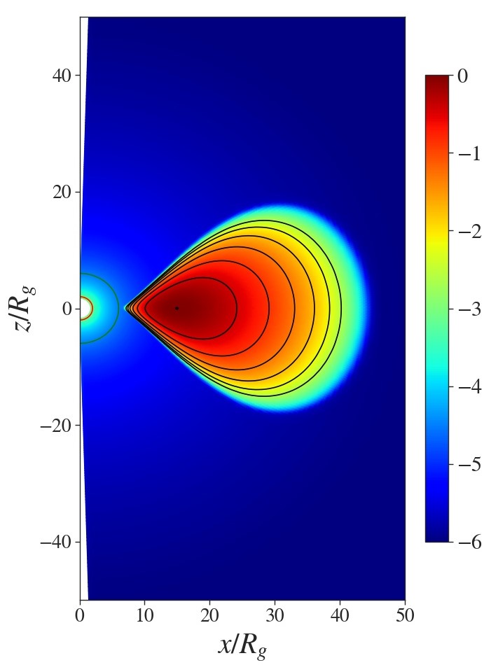
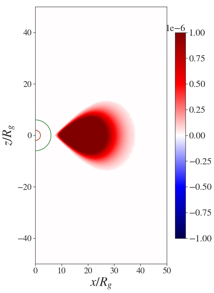
Figure 1: Initial conditions for our reference simulation. Shown is the initial distribution of the density, including contours separated by one $e-$folding scale height (logscale; upper left), the toroidal magnetic field $B_{\phi}$ (linear scale; upper right), the diffusivity $\eta$ (linear scale; lower left), and the dynamo parameter $\xi$ (linear scale; lower right).

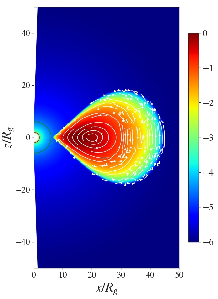
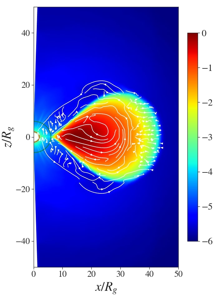
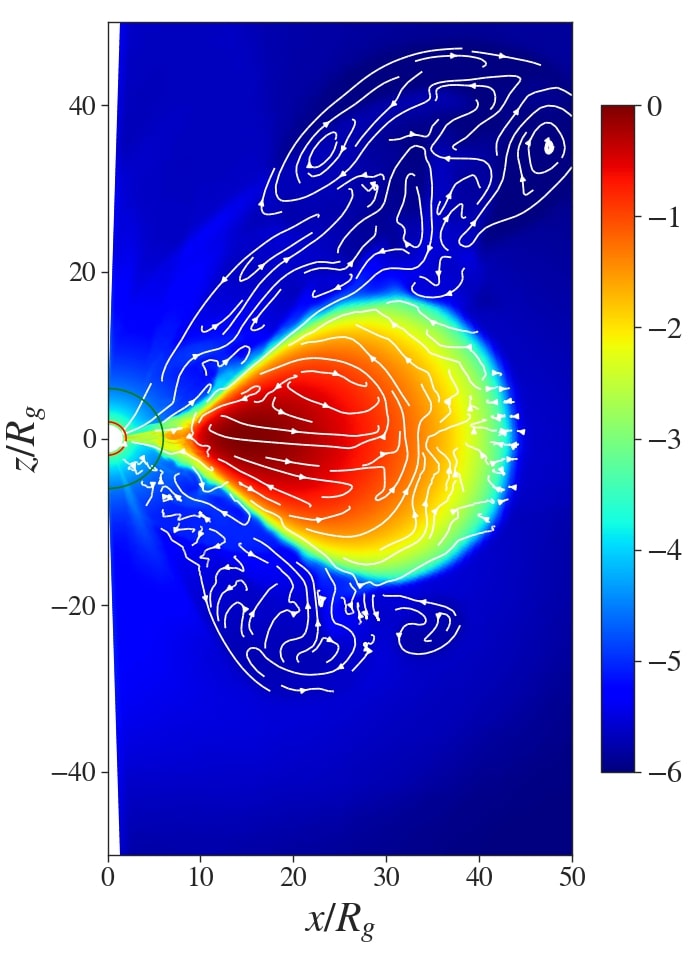
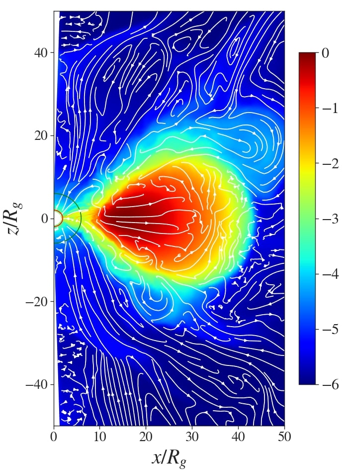
Figure 2: Generation of a dipolar poloidal field. The color gradient shows the density distribution in log scale and the white lines show the poloidal magnetic field. The initial condition starts with a toroidal field with high plasma-$\beta\sim 10^{6}$. The poloidal field appears immediately in the area where dynamo exists ($t=1$, upper left) and it evolves through $t=1000,2000$ and $3500$. This corresponds in approximately 10 rotations of the point of maximum density at $R_{\rho_{\text{max}}}=15$.

Our simulation setup for this exemplary torus simulation simT is as follows. We start the simulation with a density and internal energy distribution following the Equation of State for an ideal gas, which reads as

$$\rho=\left(\frac{(h-1)(\gamma-1)}{K\gamma}\right)^{1/(\gamma-1)},$$ (27)

where $h(r,\theta)$ is the specific enthalpy as it is calculated in Fishbone & Moncrief (1976). The torus is rotating around a Schwarzschild black hole ($a=0$) with an inner edge at $r_{\text{in}}=6$ and its point of maximum density at $r_{\rho_{\text{max}}}=15$. The internal energy is defined by the polytropic equation of state $u=K\rho^{\gamma}/{\gamma-1}$, with $K=10^{-3}$ and $\gamma=4/3$.

An initial toroidal magnetic seed field is defined inside the torus, following the density distribution ($B_{\phi}\propto\rho$) of the standard Fishbone-Moncrief torus applied in HARM (Gammie et al., 2003). This guarantees that the magnetic field is confined inside the torus. The field direction is positive in both hemispheres and it is normalized considering a plasma-$\beta_{0}=10^{6}$.

We prescribe a distribution for the magnetic diffusivity that follows the density distribution of the torus with a maximum value of $\eta_{0}=10^{-3}$. The diffusivity basically vanishes in the surrounding corona. Also the dynamo action is limited to the area inside the torus. It is constrained to an area smaller than distribution of the initial magnetic field and the diffusivity in order to avoid field generation in the corona of the torus. The dynamo parameter is constant in both hemispheres at a level of $\xi_{0}=10^{-3}$.

The parameters of our torus simulation simT are summarized in Table 1. The initial conditions for this simulation are shown in Figure 1.

We note that this setup is somewhat different from the one chosen by Tomei et al. (2020), as their initial torus is that of a so-called Polish donut (see e.g. Abramowicz & Fragile 2013) and their seed field geometry is that of poloidal loops inside the torus. With our approach we prefer to connect our simulations to the literature of HARM simulations which typically apply the Fishbone-Moncrief torus as initial condition, and While our initial setup may look similar to Tomei et al. (2020) our results cannot directly compared.

Table 1: Summary of parameters of the torus simulation run. Listed is the ID of the run; the Kerr parameter $a$ applied; the maximum magnetic diffusivity $\eta_{0}$; the initial plasma-$\beta$ and the dynamo parameter $\xi_{0}$.

run	$a$	$\eta_{0}$	$\beta_{0}$	$\xi_{0}$
simT	0	$10^{-3}$	$10^{6}$	$10^{-3}$

3.1 Field induction by a spatially constant dynamo

We now describe the field evolution of a torus induced by a mean-field dynamo in more detail.

When the simulations starts, the poloidal magnetic field appears immediately inside the torus in the area where $B_{\phi}$ and dynamo coexist. As the simulation continues, the field starts increasing in value due to the dynamo while advecting towards the black hole following partially the accretion of the torus increasing the magnetic field in the inner disk part and towards the black hole. Simultaneously, diffusivity is trying to dampen the magnetic field. In the end, the ${\cal R}_{\xi}$ determines where the field is amplified or dampened. Since $\xi$ is constant, the profile of diffusivity determines the value of $R_{\xi}$. As an example of their values, in the center of the torus the numbers are $R_{\xi}\sim 15$ while its maximum values reaches $R_{\xi}\sim 150$ in the boundaries of the dynamo distribution.

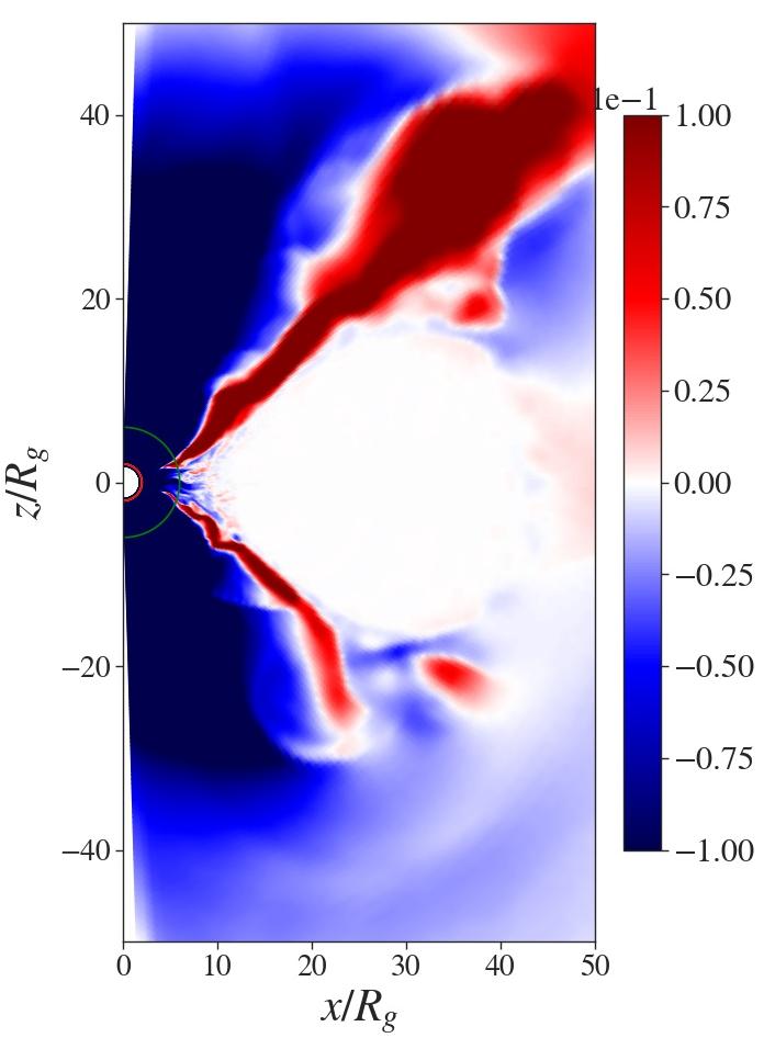
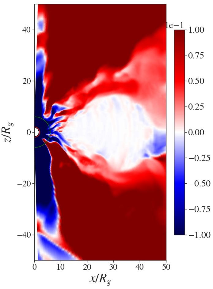
Figure 3: Distribution of the radial velocity at $t=2000$ (left) and $t=3800$ (middle) as well as plasma-$\beta$ at $t=3800$ (right) in the torus simulation. The color bars are chosen to highlight the 4 different velocity areas, such as the torus (white), the funnel flow (dark red), the torus wind (light red), and the infall (dark blue), as well as the areas of high (green) and weak (red) magnetization.

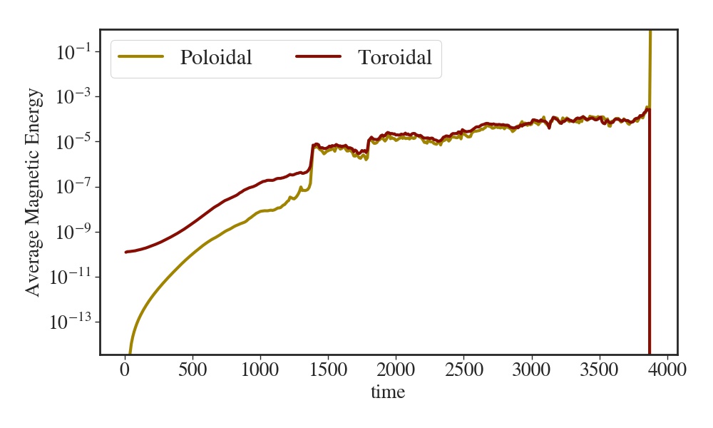
Figure 4: Time evolution of the average magnetic energy across our simulation grid for the poloidal and toroidal field component.

In Figure 2 we see the snapshots of the evolution of the poloidal magnetic field. As mentioned before, in the beginning, the field lines are restricted in the area where $\xi\neq 0$. However, they are eventually dragged along with the material that is accreted towards the black hole. At time $t=2000$, as the dynamo has been working for approximately 6 rotations of the torus center, we see a low velocity outflow being launched from the inner part of the torus. The magnetic field lines follow the low density fluid showing the first indications of the development of a jet. The launching point of the outflow is barely inside of the innermost stable circular orbit (ISCO) and can be attributed to the presence of the strong toroidal magnetic field we see in the close atmosphere of the inner part of the torus. This strong toroidal field, which has been amplified by the $\Omega$ effect of the dynamo, can increase the magnetic pressure and push material and poloidal field outwards (Lynden-Bell, 1996).

The poloidal field continues to grow up to $t\sim 3800$, but then the field close to the axis becomes too strong, resulting the code to fail to converge. At that time, both the toroidal and the poloidal components of the field have spread into the greatest part of the grid while the plasma-$\beta$ has reached values between $0.01-0.1$ inside the ISCO and around 1-10 in the outflow. Still, the torus is hydrodynamically dominated (see Figure 3).

The material accelerated in the outflow consists mainly of the floor values used by the code as background environment. We observe outflow velocities larger than $0.1\,c$ (see Figure 3). The acceleration is supported by magnetic pressure forces. This holds for the high speed floor material, but for the torus material that moves with a radial speed $\simeq 0.01$ (the light-red area in Figure 3, left) we expect that the driving is in addition also supported by gas pressure. Note also that along the axis where the toroidal field vanishes we observe infall towards the black hole.

In Figure 4 we show the evolution of the average magnetic energy for both the poloidal and the toroidal field. In both channels the energy increases over orders of magnitude until a saturation level appears around $t=1500$. There is no full saturation as beyond $t=1500$ the field energy still increases by a factor of 100-1000, however the strong increase of the dynamo action flattens substantially. The flattening is interesting insofar as we do not apply dynamo quenching in this simulation. So the dynamo seems to self-quench. This has also been seen in the literature (see below). We hypothesize that this is due to re-connection of the tangled magnetic field with time, as Figures 2 and 3 show clear evidence for an increasingly turbulent state of the magnetic field. Due to the application of resistivity, this field may physically reconnect, lowering the magnetic energy and heating the plasma.

We think that the process works in two ways. First, the dynamo-generated magnetic field can transported out of the dynamo-active area, however an area where there is still a non-negligible resistivity (basically the light red area in Fig. 1 (upper right). Since the field is tangled (see Figures 2) it will reconnect. However, the same process may happen also inside the torus. The resistivity is largest inside the torus (dark red areas in Fig. 1, right), thus, reconnection will be very efficient here. Considering this and also that the dynamo-generated field is strongest here (the $\xi$ is large), reconnection will work efficiently in lowering the net magnetic field energy.

Interestingly, this points towards a new possible channel for dynamo quenching by reconnection. Considering magnetic diffusivity, we may mostly think of diffusing away magnetic flux and by this lowering the efficiency of the dynamo. However, also reconnection is a result of magnetic diffusivity, that does naturally lowers the field energy.

3.2 The dynamo-generated torus magnetic field

The initial condition of the toroidal component of the magnetic field follows the density profile while keeping a positive sign in both hemispheres. A toroidal field is also produced by the $\Omega$ effect by differential rotation of the induced poloidal field, increasing the initial toroidal field.

The induced toroidal field changes sign in the equatorial plane, keeping its positive values in the upper hemisphere (where the radial field is negative). This results in a gradual change in the toroidal field across the torus, when the initial condition is superimposed by the newly generated field.

At time $t=1000$, the sign has changed already within the borders of the area where dynamo activity has prescribed. The change of sign of the toroidal field then continues to gradually affect also the lower hemisphere. At time $t=2000$ this transformation has almost finished, resulting in a toroidal field distribution that changes sign across the equatorial plane.

The dynamo-generated poloidal field is dominated by the radial component. Note that the direction of the radial field component also affects the direction of the poloidal field. Here we have the problem that the dynamo-generated field which is initially prescribed as a perfect dipole (with negative values in the upper hemisphere and positive values in the lower hemisphere), eventually turns into a form of stripes that show alternating positive and negative directions, which eventually result in the formation of closed magnetic loops.

This effect of inducing a layered structure of the radial magnetic field components naturally also affects the direction of the toroidal field, where we see a similar behavior in later evolutionary stages. This effect becomes apparent from $t=500-800$. At this time, the initial dipolar field geometry begins to change its topology, as we find a positive $B_{r}$ in the upper hemisphere, that was initially set to a negative radial field structure.

Similarly, this is seen in all components of the magnetic (and also in the electric field). From $t=1000$ an additional layer appears in the $B_{r}$ distribution, now with a negative value that is alternating with the previously induced positive $B_{r}$ in the upper hemisphere.

We observe this process for the whole duration of the simulation run and eventually find a completely layered magnetic field structure of alternating field direction. We note that this layered structure shows up preferentially close to the equatorial plane of the torus. Here, we also find high dynamo numbers of the turbulent dynamo exactly within previously mentioned layer. In later times this region of layered magnetic field direction spreads out over the whole torus and can eventually be found in the outflows as well. This dynamical process was also reported in Bugli et al. (2014) and Tomei et al. (2020) despite a different prescription for the symmetry of the dynamo parameter.

The time evolution and the spatial structure of the magnetic field evolving strongly reminds on dynamo waves that are generated during the kinematic phase of the mean field dynamo process. Dynamo waves are typically discussed as oscillatory solutions of the kinematic dynamo problem. The existence of such dynamo waves have been investigated early by Parker (1955) and many subsequent studies (see e.g. Weiss et al. 1984; Hughes & Tobias 2010).

Here, we solve for the dynamical dynamo problem, i.e. essentially considering the back reaction of the magnetic field generated on the gas. Nevertheless, in the early stages of the simulations, we are still in the linear regime of the dynamo action, and the field is not yet strong enough (high plasma-$\beta$) to act on the gas. The situation is thus comparable to the kinematic regime and the excitation of dynamo waves may indeed be expected. More recent studies have detected also dynamo waves in cases of high magnetic Reynolds numbers (Cattaneo & Tobias, 2014; Nigro et al., 2017). This is essential to know, as also in our simulations the magnetic Reynolds numbers ${\rm R_{\text{m}}}\equiv(vL)/\eta\simeq 1000$ can be high, assuming as a typical length scale the torus scale height $L\simeq 10$, a typical velocity $v=0.1$, and a maximum diffusivity of $\eta=0.001$ (all in code units). We note here that much of the work cited here has been done for spherical stellar dynamos. However, the case of of the relativistic torus is probably not too far from this, as compared to our studies of thin disks later on in this paper, the shear in the torus is relatively weak.

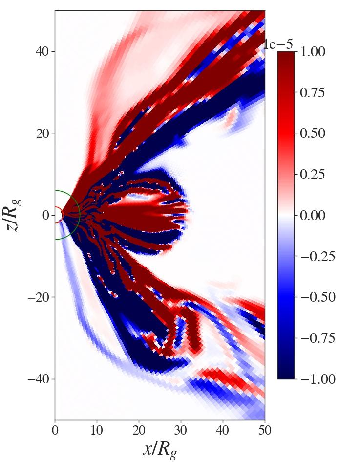
Figure 5: The radial magnetic field structure in simulation simT at time $t=2800$.

A characteristic feature of dynamo waves is that the typical time scale of the fluctuations is similar to the diffusion time scale (see e.g. Giesecke et al. 2005 for spherical $\alpha^{2}$-dynamos). For the simulations presented in this section, this is indeed the case. With a maximum diffusivity $\bar{\eta}\simeq 10^{-3}$ in the torus and the typical length scale in the torus $\Delta R\simeq 1$, we calculate a global diffusion time scale of $\tau_{\rm diff}=(\Delta R)^{2}/\bar{\eta}\simeq 10^{3}$ in code units. This is indeed similar to the time scale we measure for the global variations of the dynamo-induced field structure. Although the values considered are some rough estimates and vary drastically over the torus, we may see this correlation as a hint for dynamo waves in our simulations.

Even at late stages of our simulation, the plasma-beta in the torus is of the order of 100-1000, thus the dynamo still acts in the kinematic regime. Nevertheless, the generated magnetic field has expanded and fills the space between the rotational axis and the torus. Here, the plasma-beta is lower $\beta\simeq 0.1$, and the evolution is dominated by the magnetic field.

Overall, we see indication that dynamo waves are excited during the initial stages of the magnetic field evolution on our torus model simulation. This is in particular demonstrated in Figure 5 that shows the generation of a layered structure of an anti-aligned field (here shown by the by the radial field component. This figure show striking similarities to Figure 3 in Tomei et al. (2020), who, however, plot the magnitude of the field only, not its direction.

3.3 Comparison to literature studies

At this point it is interesting to compare to the existing litrerature, in particular to the simulations of Bucciantini & Del Zanna (2013) on which the mean-field dynamo closure of our code is based and the follow-up papers (Bugli et al., 2014; Tomei et al., 2020) . As mentioned above, while the geometry of the latter two approaches look similar, the actual initial conditions are quite different. Our initial torus structure follows the Fishbone-Moncrief solution (Fishbone & Moncrief, 1976) that is applied in previous HARM simulations, while their torus follows a different prescription. Overall, our initial torus extends to $r\simeq 45$, while Bugli et al. (2014) consider a quite smaller structure with $r<10$. The Polish donut torus solution applied in Tomei et al. (2020) appears to be much larger, however of the full grid of $r<100$ only the innermost radii $r<20$ are shown.

Also the initial field structure and the diffusivity distributions are different.

Given the different initial setup a quantitative comparison to our results is not possible. However, we observe similar structures evolving from our dynamo. Similar to Tomei et al. (2020) we observe the generation of bipolar magnetic "arms" around the inner edge of the torus. Also, authors claim to detect dynamo waves being dragged towards the black hole by accretion.

We show the 2D magnetic field evolution at a somewhat longer time step (in codes units $t=3500$ vs. $1608$ in Tomei et al. 2020). Therefore we are able to follow the expansion of the generated magnetic flux away from the torus and towards the rotational axis. At $t=3500$ we indeed see a strongly magnetized axial region, that may allow for Blandford-Znajek jets in case of a rotating black hole.

We note however that the dynamical evolution of the torus and also of the dynamo action is quite faster in their smaller sized torus setup. The 6 periods of torus orbits they show in their 2D images (and the 12 orbits they actually simulated) are calculated considering a radius of the torus center of $r_{c}=12$, while the center of our torus is further out $r_{c}=15$, resulting in about a factor 2 longer rotational periods for our torus center and thus a similarly longer evolution time. The advection time of magnetic flux towards the axis is not affected by that, however.

Interestingly, Tomei et al. (2020) find a (second) saturation phase of field amplification even without quenching their mean-field dynamo, probably due to the accretion dynamics together with an equipartition state of the fluid system

In our simulations we also find a transition to a saturation state, more accurately, a strong break in the growth rate of both field components (see Figure 4 and our corresponding discussion above). Tomei et al. (2020) argue that the change is happening at the time when local equipartition is reached. We may confirm this as close to the inner edges of the torus we also find equipartition at this stage (see Figure 3 upper right for a latter evolutionary stage). However, we hypothesize that the change in slope for the increase of magnetic energy can also be due by reconnection of the tangled magnetic field that is produced by the dynamo action (see discussion above).

We do not find the second saturation phase claimed by Tomei et al. (2020). The time scale of our simulation would be sufficiently long, however, since our simulation setup is different, in particular the dynamics of initial torus, a proper comparison cannot be made here. We note again, that measured in orbital periods of the torus, the evolutionary time of their torus is somewhat longer, and we might therefore have not yet reached the second saturation phase (if this phase would be present at all in our setup).

The poloidal field structure derived by Tomei et al. (2020) is visualized by showing the magnetic energy distribution. Here, we also show poloidal field lines that can better trace the small-scale structure of the field, as well as the field direction.

To see the very structure of the vector field, meaning the geometry of the magnetic field lines and the distribution of the magnetic flux, is essential for understanding the jet launching process. For example, for considering magneto-centrifugally driven disk winds, the field inclination is important (Blandford & Payne, 1982).

So far, for the test simulations provided in the literature of GR-MHD dynamos (Bucciantini & Del Zanna, 2013; Bugli et al., 2014; Tomei et al., 2020), field lines for the resulting magnetic field structure are only given for the case of a neutron star dynamo (see Section 5.2.4 of Bucciantini & Del Zanna 2013). Thus we cannot compare our field structure in detail with the existing literature. This would have been interesting as the essential effect of the dynamo action is in particular to generate poloidal magnetic flux along the disk.

4 Initial setup for a thin disk dynamo

Here we describe the initial conditions for our dynamo simulations considering a thin accretion disk. The simulation grid extends from just inside the event horizon to a outer radius of $r=80$. The radial and polar dimensions are based on the original grid of HARM The numerical grid size used is $256\times 256$.

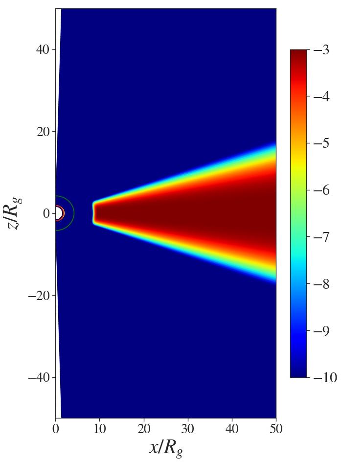
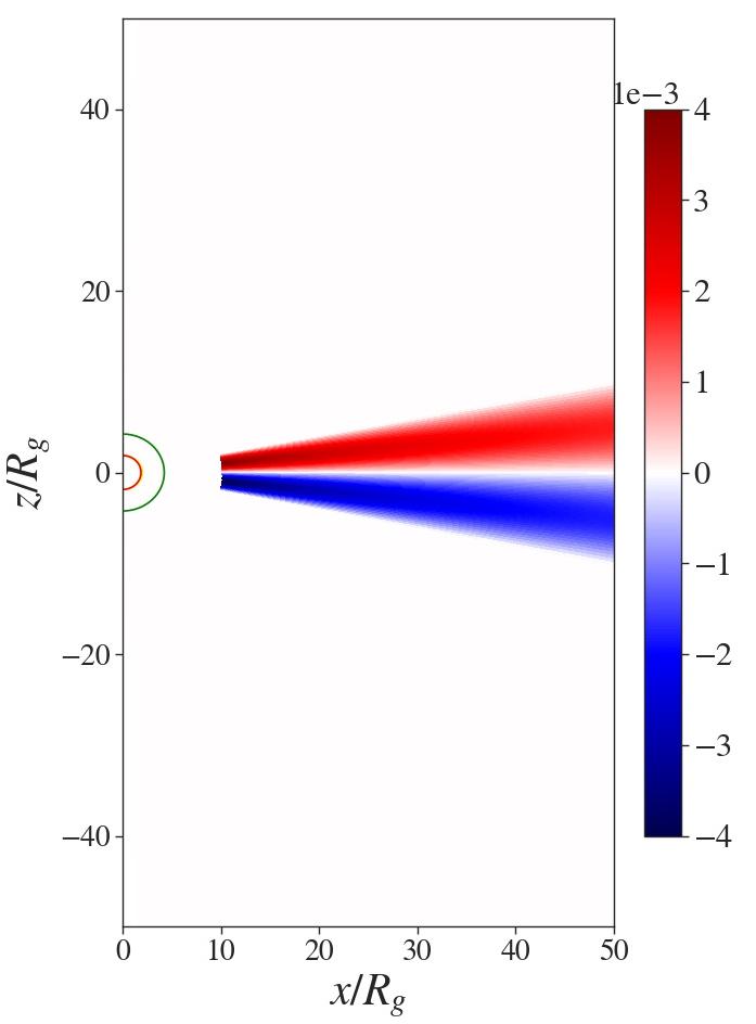
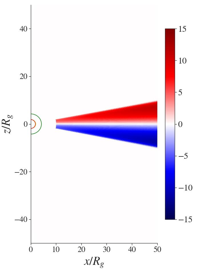
Figure 6: Distribution of the magnetic diffusivity $\eta$, the dynamo parameter $\xi$, and the magnetic Reynolds number ${\cal R}_{\xi}$. Representations are in log scale.

The simulation is initiated with a thin accretion disk with a density distribution similar to the one used by Vourellis et al. (2019)

$$\rho(r,\theta)=\left[\frac{\Gamma-1}{\Gamma}\frac{r_{in}}{r}\frac{1}{\epsilon^{2}}\left(\sin\theta+\epsilon^{2}\frac{\Gamma}{\Gamma-1}\right)\right]^{1/(\Gamma-1)},$$ (28)

which is connected with the gas pressure by an ideal equation of state $P=K\,\rho^{\gamma}$. The aspect ratio of the disk is $\varepsilon\sim 0.1$. The disk is surrounded by a corona with an initial density and pressure given by

$$\rho_{\text{cor}}\propto r^{1/(1-\Gamma)},\quad\quad p_{\text{cor}}=K_{\text{cor}}\rho_{\text{cor}}^{\Gamma}.$$ (29)

We choose $K=0.001$ for the disk and for the corona $K_{\text{cor}}=1$ and force an initial pressure equilibrium between he disk and the corona implying a density jump between corona and disk surface. When the simulations starts, the initial corona starts collapsing, and is then replaced by the floor values for density and pressure, described by a broken power (Vourellis et al., 2019).

The disk is given an initial rotation profile following Paczyńsky & Wiita (1980) as

$$\tilde{u}^{\phi}=r^{-3/2}\left(\frac{r}{r-R_{\text{PW}}}\right),$$ (30)

where $R_{\text{PW}}$ is a constant, here set equal to the gravitational radius $R_{\rm g}$.

The initial seed magnetic field is purely radial and is prescribed only inside initial disk. Having a radial field has the advantage of a vanishing shear between the rotating disk and disk corona. We have also run simulations starting with a purely toroidal initial field, however, resulting in a similar long-term magnetic field evolution. The initial magnetic field prescription involves purely radial magnetic field lines that converge in the black hole horizon, implemented numerically via the magnetic vector potential,

$$A_{\phi}(r,\theta)\propto\exp{\left[-\frac{1}{2}\left(\frac{1}{0.05\tan\theta}\right)^{2}\right]}.$$ (31)

The strength of the seed field is defined by the choice of plasma-$\beta=10^{6}$.

In the simulations we apply a profile of the magnetic diffusivity that is somewhat modified compared to Vourellis et al. (2019), but similar to the dynamo simulations by Stepanovs et al. (2014). This profile has a constant plateau across equatorial plane, but then quickly drops in polar direction for $\theta<85^{\circ}$ and $\theta>95^{\circ}$,

$$\eta(r,\theta)=\eta_{0}\exp\left(-100\frac{\left(\pi/2-\theta\right)^{4}}{\arctan(\chi_{\eta}\cdot\varepsilon)}\right),$$ (32)

where $\eta_{0}$ is the (initial) maximum value and $\chi_{\eta}=3$ characterizes the scale height of the diffusivity distribution. The profile of the mean-field dynamo follows Stepanovs et al. (2014),

$$\xi(r,\theta)=\xi_{0}\frac{1}{\sqrt{r/r_{\text{i}n}}}\sin\left(\frac{\pi}{\chi_{\xi}\cdot\varepsilon\cdot\tan{\theta}}\right),$$ (33)

where $\chi_{\xi}=1$ is a characteristic scale height for the dynamo. The latter is an important constraint, as by choosing $\chi_{\xi}<\chi_{\eta}$ we ensure that the dynamo action is always enclosed in the resistive area. Otherwise we may consider arbitrarily large dynamo numbers (see below). Furthermore, the purely resistive outer layers of the disk will allow for easier launching and mass loading of disk winds (Vourellis et al., 2019). In Figure 6 we show the distribution of the magnetic diffusivity $\eta$, the dynamo parameter $\xi$ and Reynold’s number ${\cal R}_{\xi}$.

5 The accretion disk dynamo

Our paper focuses on the generation of a strong poloidal flux anchored to a thin accretion disk. As reference simulation we consider the case of a Schwarzschild black hole. A very low radial magnetic field with $\beta=10^{6}$ is applied as a seed field for the dynamo action, following the (non-relativistic) approach by Stepanovs et al. (2014); Fendt & Gaßmann (2018). Note that our initial disk structure is not in complete equilibrium with the black hole (different from the non-relativistic simulations). Thus, during the initial evolution the disk will adjust on the relativistic potential, causing deviations on the seed field from the perfectly radial structure. These deviations, however, are minimal and significantly smaller that the magnetic field that is generated by the dynamo later on. Simulations with a different initial field structure (e.g. a toroidal field) lead to the same magnetic structure in the saturation phase.

Table 2: Summary of thin disk simulation runs. Listed is the ID of the run; the Kerr parameter $a$ applied; the maximum magnetic diffusivity $\eta_{0}$, typically located at the inner disk radius; the maximum (initial) dynamo parameter $\xi_{0}$; and the quenching parameter $\beta_{\textrm{e}q}$, corresponding to an equipartition field strength, beyond which dynamo action is strongly quenched.

run	$a$	$\eta_{0}$	$\xi_{0}$	$\beta_{\textrm{e}q}$
sim0	0	0.001	0.004	1000
sim1	0	0.001	0.004	100
sim2	0	0.001	0.004	10
sim3	0	0.001	0.004	1
sim0.1	0.9	0.001	0.004	1000
sim1.1	0.9	0.001	0.004	100
sim4	0	0.001	0	-
sim5	0	0.001	0.004	no quenching

Figure 7 shows exemplary evolution of the poloidal magnetic field together with the evolution of the density for reference simulation sim1. When the simulation starts, the initial radial structure of the magnetic field inside the disk is evolved by the dynamo action. The geometry of this dynamo-generated field does not follow a clear dipolar structure.

In addition to the dynamo action, the hydrodynamic turbulence that develops in the disk amplifies the state of the magnetic field. We note here that this turbulence is a consequence of the existence of an anti-aligned poloidal field structure that further develops when the poloidal field is advected towards the horizon. The field geometry close to the horizon (say for $r<5$) resembles that of the Wald solution (Wald, 1974; Komissarov, 2005). With our resistive approach, this leads to strong reconnection events that affect the mass loading of the outflow as well as the accretion of material, and also the foot point of the magnetic field lines that guide the outflow (see also Vourellis et al. 2019).

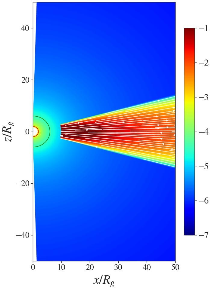
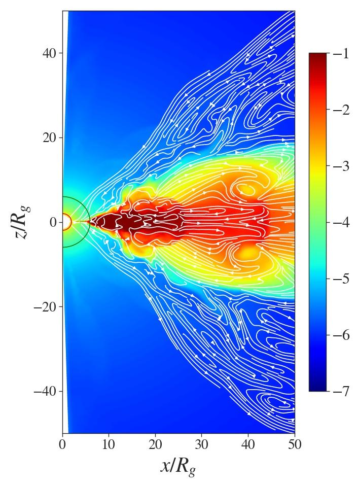
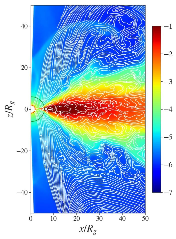
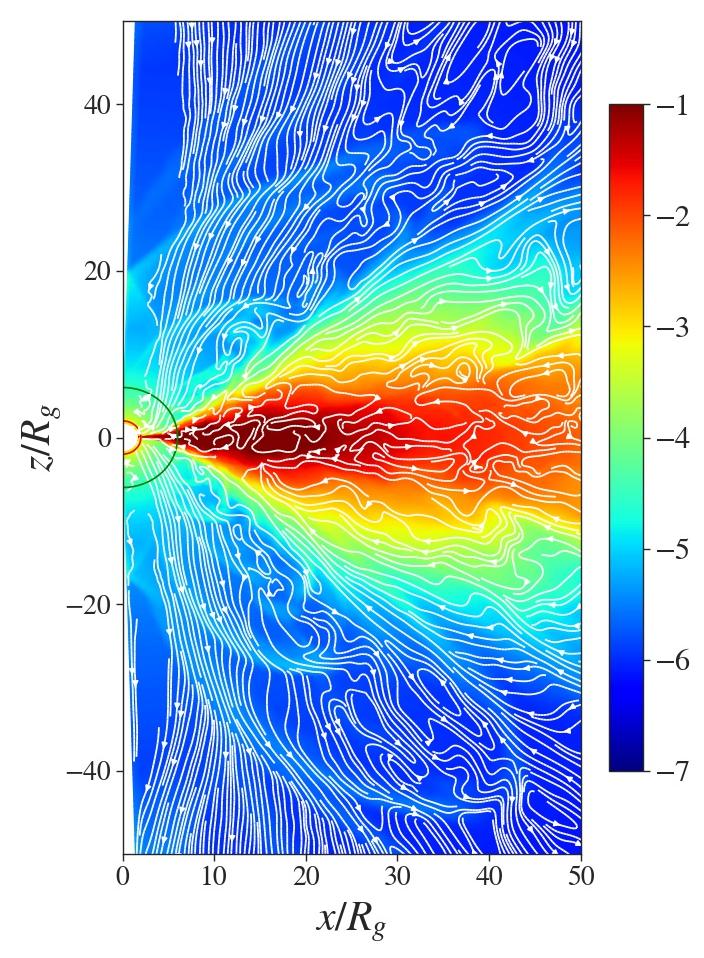
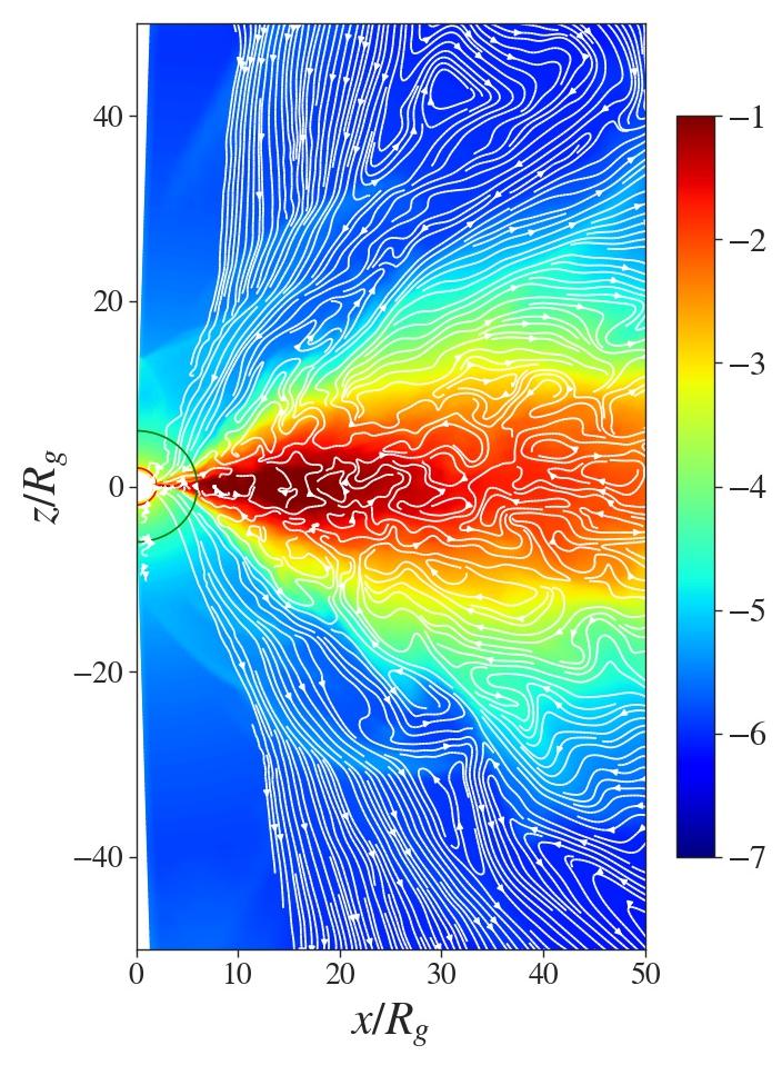
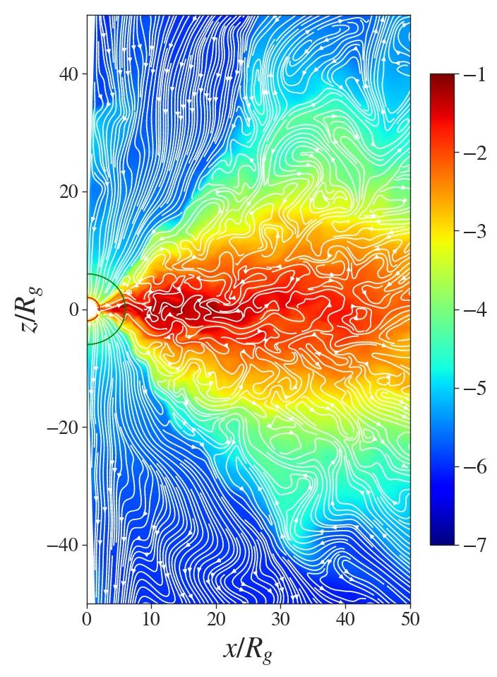
Figure 7: Evolution of the disk density and the poloidal magnetic field (white lines) for simulation sim1 at times $t=\left(0,1000,3000,6000,9000,12000\right)$. The red line around the $(0,0)$ point is the event horizon and the green line denotes the radius of the ISCO.

We do not expect the MRI to be detected in our simulations. In fact our resolution would be almost sufficient to resolve the some of the large wave modes. So while the MRI might potentially be observed in an ideal MHD study, for resistive MHD the excitation of the MRI modes is severely damped. Here, we refer to Fleming et al. (2000) and Longaretti & Lesur (2010) who investigated in great detail the effect of resistivity on the evolution of the MRI. Qian et al. (2017), investigating the role of the MRI in a general relativistic torus in resistive MHD came to the conclusion that the MRI is more and more damped for increasing level of resistivity (although applying a lower resolution).

As soon as the dynamo-induced magnetic field is strong enough to remove angular momentum from the disk, accretion sets in. With accretion going on, the newly generated field is advected towards the black hole. In the last stage of the simulation the environment close the black hole is strongly magnetized by a poloidal field with a dipolar configuration. However, at larger radii and especially inside the disk, at the time scales investigated, the dynamo has not yet generated a clear structure that provides a large scale magnetic flux. Note that these simulations are quite CPU-intensive, and the time scales we are reaching here of about $t=10000$ corresponds to about 150 inner disk rotations. In contrast, the non-relativistic disk dynamo simulations (Stepanovs et al., 2014; Fendt & Gaßmann, 2018) reach up to several 100.000 disk rotations.

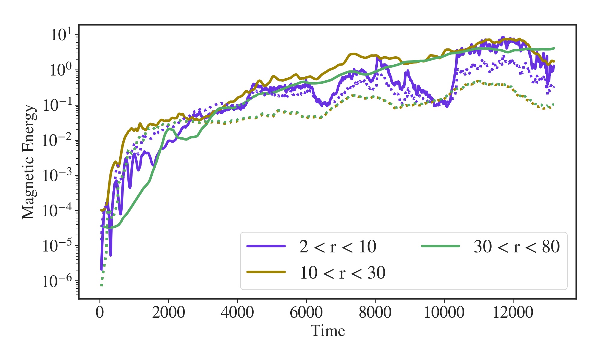
Figure 8: Evolution of the poloidal (solid line) and toroidal (dotted line) magnetic energy integrated between three different radii inside the accretion disk for simulation sim1.

5.1 The evolution of the dynamo generated magnetic field structure

We now discuss the magnetic field structure that is generated by the disk dynamo (see Figure 7) and how its geometry and field strength depends on the parameters that trigger the dynamo process, namely the strength of the dynamo $\xi$, the disk diffusivity $\eta$ (in combination the dynamo number), and the quenching parameter $\mu_{\rm eq}$.

Figure 8 shows the evolution of the integrated poloidal and toroidal magnetic energy in three different regions (distinguished by their inner and outer radius). We emphasize that for later times the dynamo induced poloidal field remains substantially higher than the toroidal field component. This again points towards an efficiently working $\alpha$-dynamo, since only the $\alpha$-process can amplify the poloidal field component.

For the innermost part of the accretion stream between the black hole horizon and the initial inner disk radius $(2<r<10)$, the initial magnetic energy vanishes (since the seed field is confined inside the disk only) and then quickly increases due to the dynamo-generated field. When the disk starts evolving, meaning that accretion of disk material sets in, the magnetic field is getting advected towards the black hole. Due to the unsteady accretion process, also the advected magnetic energy is varying. Indeed, the initial variations in magnetic energy we find, do correlate with the spikes in the accretion rate (see top panel of Figure 9). After $t\simeq 2000$, the increase of the magnetic energy continues, but with a smaller slope and after $t\simeq 6000$ we see indication of a saturation of the dynamo action as the slope of the magnetic energy increase decreases even further to the point it is almost constant. Still, we do not reach a constant value, as at $t\simeq 10000$ there is another sudden increase in the magnetic energy that is coinciding with another strong accretion event.

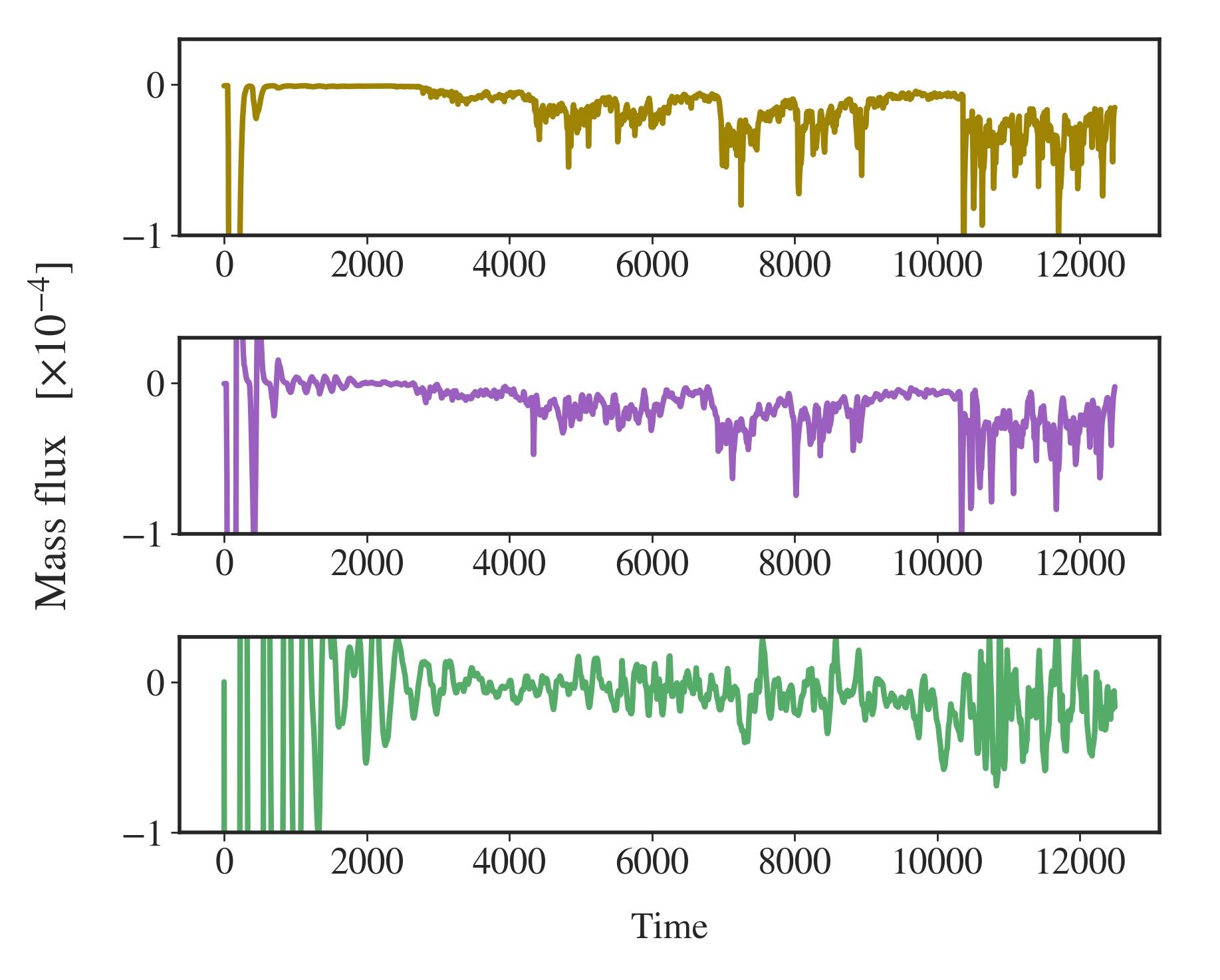
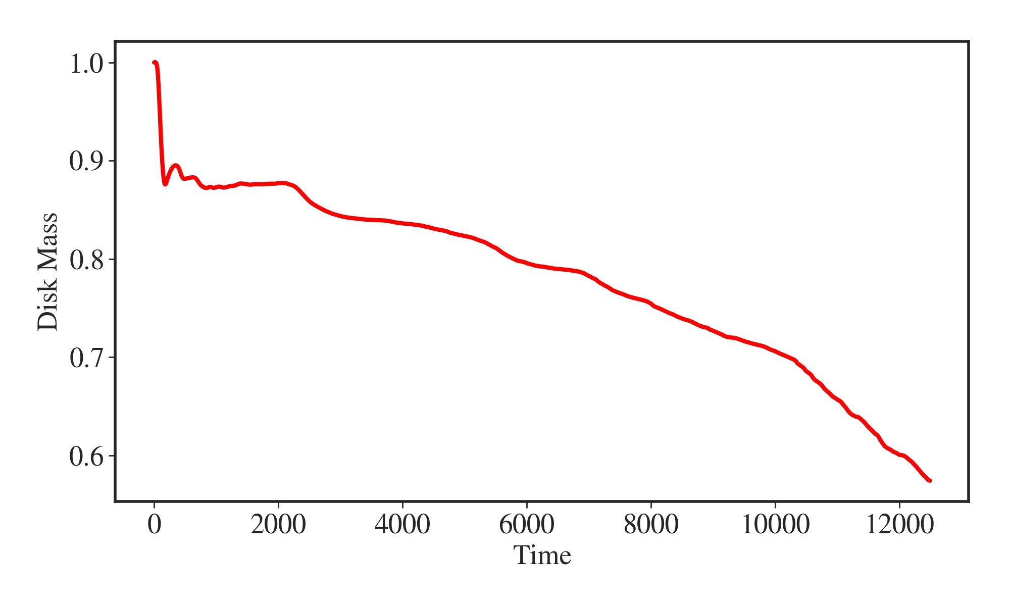
Figure 9: Evolution of mass flux rate measured at at $r\sim(3,6,11)$ (top) and normalized disk mass (bottom) for polar angles $75^{\circ}<\theta<105^{\circ}$ for simulation sim1. The negative values denote the accretion rate. The mass flux is also normalized with the initial disk mass.

At larger disk radii the time evolution of the magnetic energy looks somewhat different. The initial variations do not appear, as the accretion process works smoother in these areas. However, the overall behaviour of the magnetic energy is similar to the innermost disk. Again, at the beginning the energy increases much faster for the middle part $(10<r<30)$ but after $t\simeq 3000$ the disk magnetic energy is almost the same for both regions and slightly larger than the energy in the innermost part. After $t\simeq 10000$, with the sudden energy increase from the inner part, the energy in all three radii is approximately the same. The comparison of the magnetic energy content in these disk areas of course depends on the choice of the integration areas. What we learn from this comparison is that the disk dynamo works similarly efficient over almost the whole disk. Further, the slope of the magnetic energy growth is comparable between these areas, indicating a well posed setup for the disk dynamo, in particular, a direct coupling between the processes of accretion, ejection and dynamo action.

Figure 10: Plasma-$\beta$ at simulation times $t=4370$ (top) and $t=12000$ (bottom), considering the poloidal (left) and the toroidal (right) magnetic field component, respectively, for simulation sim1.

Figure 10 shows distribution of the plasma-$\beta$ for the poloidal and the toroidal magnetic field components at two different time steps for simulation sim1. Obviously, due to the dynamo activity, the plasma-$\beta$ decreases with time - first in inner disk area and later also in the main disk body. Also the disk wind that is launched at later time carries a low plasma beta. Overall, the toroidal magnetic field component is dominating. This has been observed also in Vourellis et al. (2019) for a magnetic field that is initially prescribed and is consistent with the literature of GRMHD disk simulations. For the time scales considered here, this tells us that the differential rotation ($\Omega$ effect) still dominates the turbulent dynamo ($\alpha$ effect). At $r\sim 15$ along the equatorial plane the dynamo number characterizing differential rotation is ${\cal R}_{\Omega}\approx 59$, while the maximum $\xi$ dynamo number ${\cal R}_{\xi}$ does not exceed 13 (see Eq. (21)).

However, we see that the plasma-$\beta$ measured in the inner part of the disk and in the accretion funnel do slightly increase during the later times of the simulation. This is a direct effect of the quenching mechanism we implemented. In addition, the magnetic field becomes quite entangled in the later stages of the simulation (see last panels of Figure 7). As a consequence, there exist further effects that can lead in the dissipation of the magnetic field, in particular magnetic reconnection. What can be clearly seen from the figure is that exactly those areas of low plasma-$\beta$ are also the areas from which strong outflows develop from the inner disk (see also Section 5.4 below).

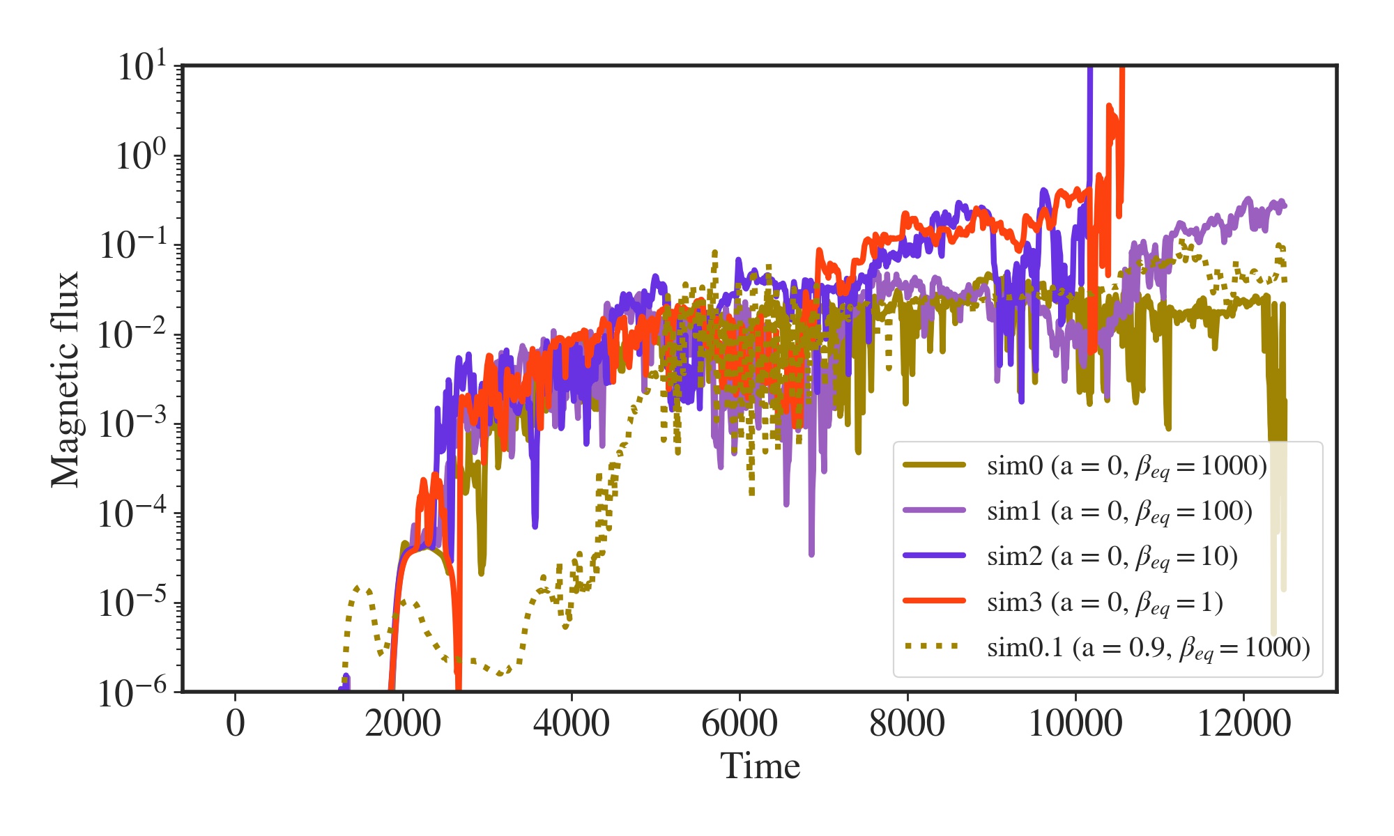
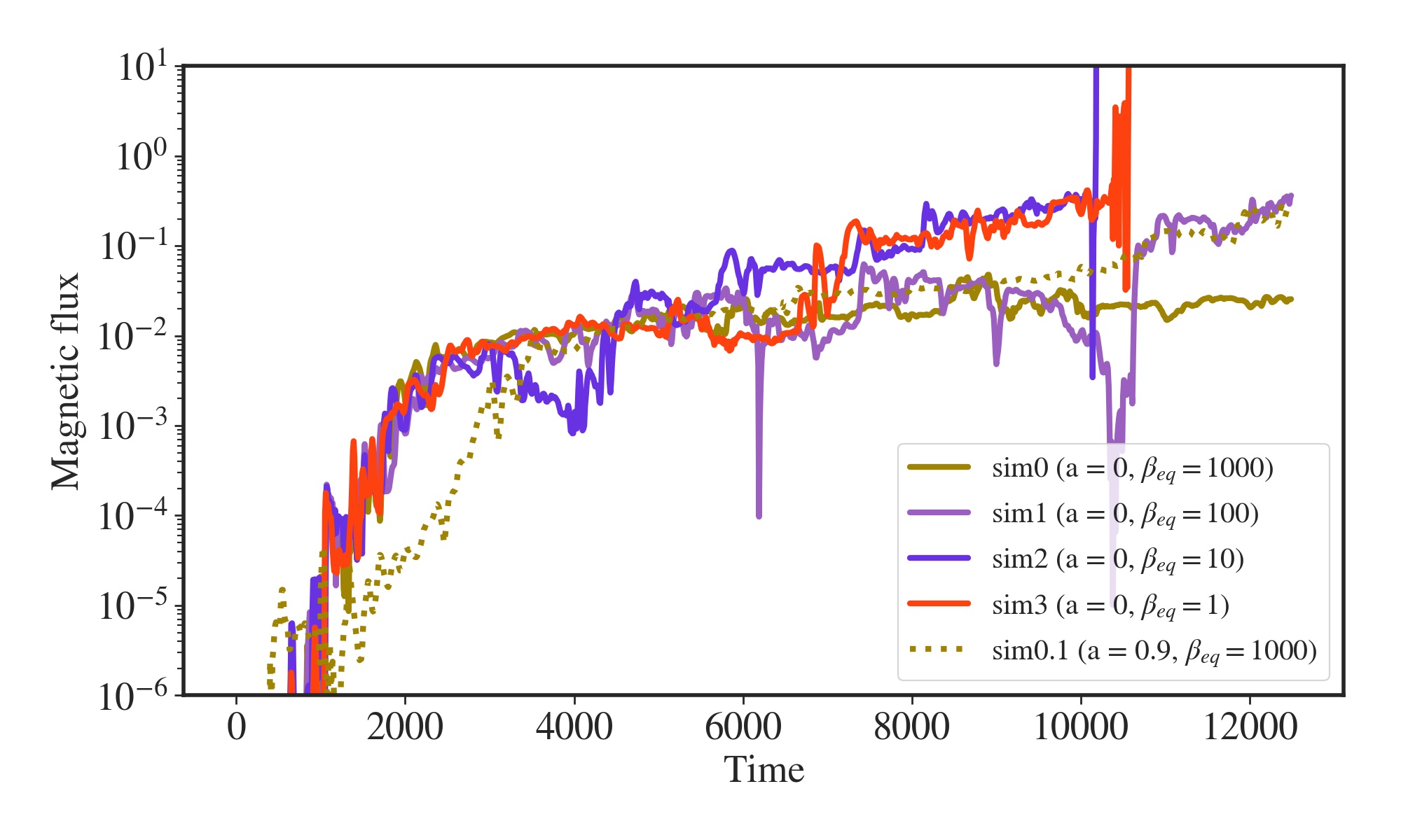
Figure 11: Time evolution of the absolute integrated magnetic fluxes. Shown is the magnetic flux from the disk surface (top), thus integrated radially along the disk surface, and the flux through a circular cross section over the polar angle $0^{\circ}<\theta<70^{\circ}$ at radius $r\sim 11$ and its corresponding areas in the lower hemisphere (bottom). Simulations with different levels of dynamo quenching and Kerr parameter are considered.

An essential condition for jet launching is a sufficient magnetic flux of the jet source, synonymous for a large-scale open magnetic field structure. As already briefly mentioned, although we may measure a substantial (poloidal) magnetic energy $\propto B_{\rm p}^{2}$ in the disk, the poloidal magnetic flux $\int\vec{B}_{\rm p}d\vec{A}$ may vanish on average, if the field is strongly tangled.

It is therefore interesting to see how the magnetic flux evolves that is generated by our disk dynamo. This is shown in Figure 11 for simulations with different Kerr parameters and quenching thresholds. Here we choose two different representations of the absolute integrated magnetic flux. One option is to integrate along a circle of constant radius (lower panel) and the other is to integrate along the disk surface (upper panel), using the $B_{r}$ and $B_{\theta}$ components of the magnetic field, respectively. Note that radius of the circle of $r=11$ is chosen such that it measures the magnetic flux close to the black hole which potentially may launch a Blandford-Znajek jet. The angle for the integration is chosen so that we avoid to account for flux from inside the disk where the field is more entangled.

The increase in magnetic flux is similar to the time evolution of the magnetic energy (see Figure 8). Differences are due to the fact that when integrating the cumulative magnetic flux $|\int\vec{B}_{\rm p}d\vec{A}|$, we effectively average over fluxes in opposite directions, as discussed above.

This clearly demonstrates that our disk dynamo also generates a substantial magnetic flux when generating magnetic energy (see Figure 7 showing indeed large-scale open poloidal field lines). Interestingly, we find that all dynamo simulations evolve with an initially very similar behaviour. At the later evolutionary stages they, however, diverge, due to the different quenching threshold they obey. Simulation sim0 keeps an almost constant magnetic flux during its final part, while for simulations with a higher quenching threshold the flux increases with a steeper slope. Simulations sim2 and sim3 end earlier due to the higher magnetization levels that is allowed by the quenching. Simulation sim0.1 that considers a highly spinning black hole, also provides an ever increasing magnetic flux over the simulation time, however, the dynamo effect is somewhat delayed.

For comparison, we have also performed test simulations sim4 without any dynamo action and sim5 without quenching. As expected, in simulation sim4 the initial radial field structure is conserved while slightly expanding in the surrounding disk corona. Minor weak outflows can be detected from the disk surface that can be attributed mostly to the local force balance between the disk vertical pressure gradient (magnetic pressure is negligible here) and the vertical gravitational force (induced by the black holes metric). In simulation sim5 the magnetic field develops as in simulation sim3, however, the lack of a quenching mechanism generates a magnetic field that becomes extremely strong and that leads the code to crash rather early. A similar behavior was also observed by Tomei et al. (2020). Both simulations, sim4 and sim5 may serve as reference for further test simulations of our implementation of the dynamo and the dynamo quenching.

5.2 Disk evolution - magnetic field and mass fluxes

We now investigate the evolution of the accretion disk, in particular the mass accretion rates, in more detail. Figure 9 (top) show the normalized mass flux through surfaces of constant radius $r=(3,6,11)$. We have selected a slice between $75^{\circ}<\theta<105^{\circ}$ in order to account for the initial disk structure and the evolution of the disk.

Due to the weak seed field, the initial evolution is basically hydrodynamic. While the initial radial structure of the magnetic field is ideal for angular momentum removal from the disk material, its strength is too low in order to have a big impact.

We find that right in the beginning of the simulation, the accretion rate shows large variations. This is due to the lack of a perfect vertical hydrodynamic equilibrium in the disk. This leads to distortions in the disk structure, and to episodic accretion events of material that has moved inside the ISCO (note the initial position of the inner disk radius is at $r=10$, well outside the ISCO). The inner part of the disk is quickly advected and when it crosses the marginally stable orbit it disconnects from the disk and falls in the black hole leaving a “gap” behind it which quickly fills with material from the remaining inner part of the disk. The initial radial shape of the initial magnetic field supports the advection of disk material towards the black hole, however, as mentioned above, this field is not dynamically important. On the other hand, the motion parallel to the poloidal field also implies that no magnetic flux is advected initially.

The episodic accretion is repeated several times depending on the disk radius (see the accretion spikes in Figure 9, top). Further out along the disk, the accretion peaks correspond to disruptions that appear at the disk surface displacing disk material (see Figure 7, top middle panel). This is a common consequence of the dynamics of the this disk in the relativistic environment (Vourellis et al., 2019).

Around time $t\simeq 2000$ the disk structure settles just outside the marginally stable orbit resulting in a more continuous accretion rate. At this time, the initial seed magnetic field starts being modified by the dynamo leading to initial weak outflows launched from the accretion funnel between the marginally stable orbit and the black hole. The outflows drag the magnetic flux with them, developing a vertical magnetic field component which then contributes to establish a smoother accretion rate. We will later discuss the onset and evolution of these outflows in more detail (see Sect. 5.4).

We find the strongest accretion rates after $t\sim 10000$. We understand this is essentially caused by the interplay between the dynamo activity and dynamo quenching (see Section 5.3). The weak outflows mentioned above remain present also during the second evolutionary phase, however, showing a time variation in velocity and mass flux. Within the accretion disk the magnetic field is substantially entangled, forming loops that reconnect with each other. The disk starts expanding in the vertical direction, but not yet developing any strong disk wind.

After $t\sim 10000$ we notice an increase in the accretion rate that coincides with an increase in the magnetic field strength close to the black hole. This is the point in time when the dynamo quenching is not sufficient to stop the magnetic field from increasing further mainly due to the radial limits within which it is defined. Note that the dynamo action and its quenching is defined only for $r>10$, which is located inside the accretion disk. When the magnetic field is advected, the magnetic flux in the black hole magnetosphere increases along with the magnetization, but this area is neither dynamo-active nor affected by quenching. The strong field of the black hole magnetosphere results in divergences in the integration of the equations which eventually lead to the termination of the simulation.

When the disk field becomes advected, these field lines also populate the area along the rotational axis resulting in a strong axial magnetic field that could potentially lead into a Blandford-Znajek-driven outflow (in the case of a rotating black hole, see Sect. 5.5).

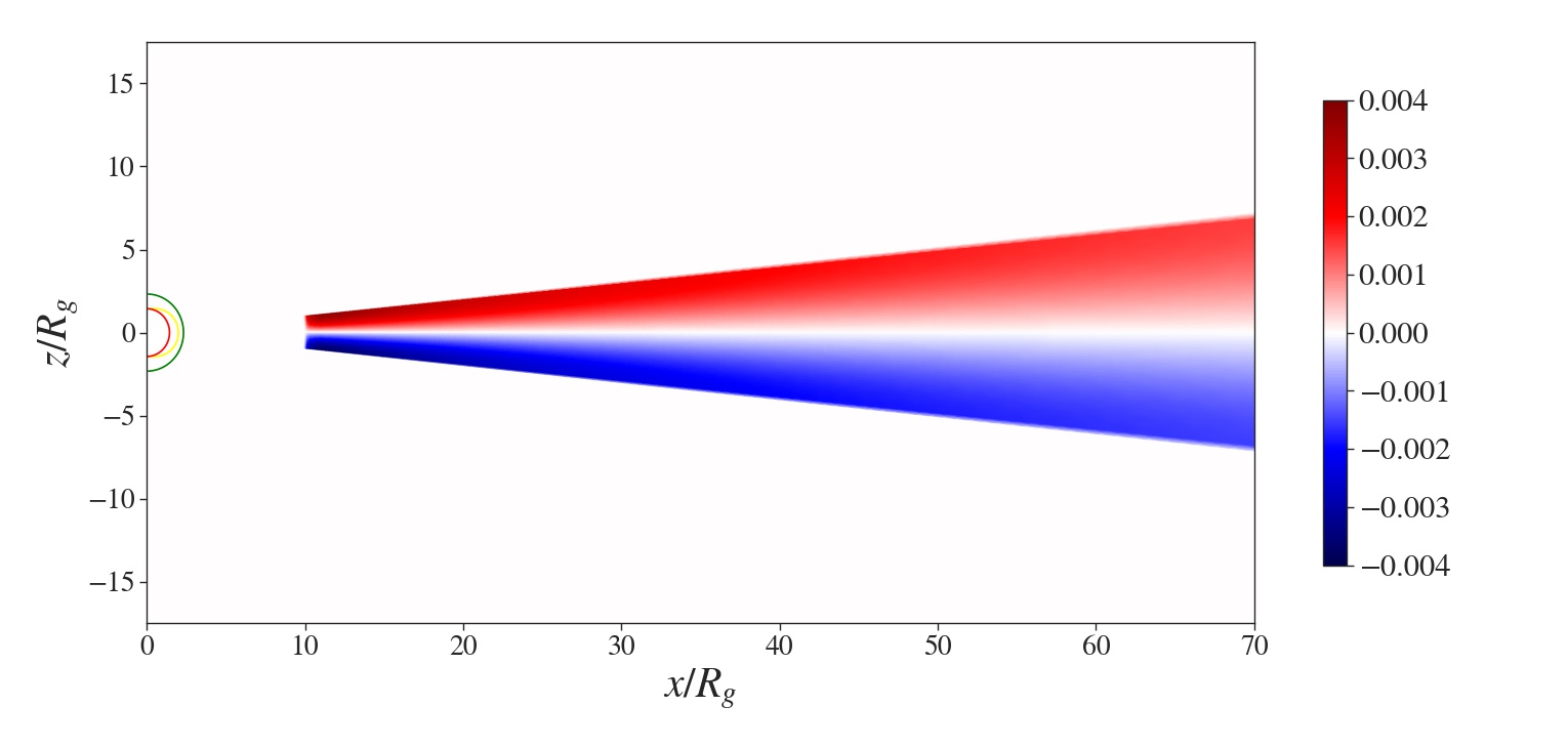
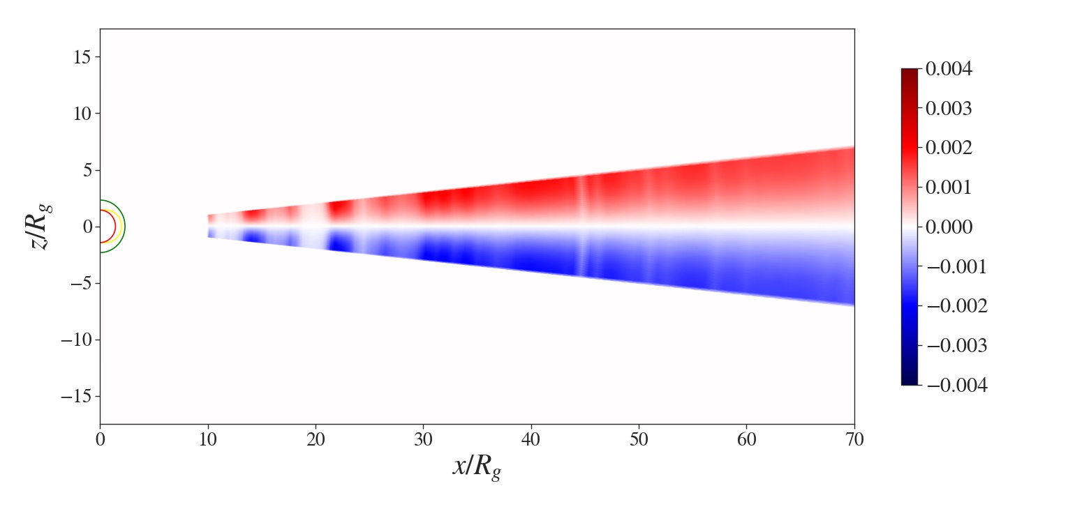
Figure 12: The distribution of the dynamo parameter $\xi$ and its variation due to quenching for simulation sim0.1 at times $t=1000,12000$.

5.3 Dynamo quenching

For completeness we briefly show the evolution of the dynamo quenching. After an initial evolutionary phase, the magnetic field continues to increase in both the poloidal and the toroidal component. However, the toroidal component is undergoing an extra amplification due to the differential disk rotation (the $\Omega$-effect). This later evolution is not as rapid as the initial boost due to the dynamo quenching that starts mitigating the dynamo effect. The dynamo quenching follows Equation (23) which for simulation sim1 has $\mu_{\textrm{e}q}=1/\beta_{\textrm{e}q}=0.01$. This implies that as the plasma-$\beta$ inside the disk decreases from the initial value of $10^{6}$ to an actual value of 100, the quenching becomes stronger.

Even for a plasma-$\beta=1000$, in our parameter setup the dynamo action is already quenched by $\sim 11\%$ and by the time when plasma-$\beta=100$ the dynamo parameter will be half of its initial value. Note that the dynamo quenching works locally, defined by the local vertically averaged disk magnetization. Depending on this, the actual strength of the dynamo tensor is quenched.

This is shown in Figure 12 where we show the distribution of the dynamo-$\xi$ for two exemplary time steps for simulation run sim0.1 with a rapidly rotation black hole. While at $t=1000$ the dynamo still works at its initial strength, at $t=12,000$ quenching is clearly seen at certain disk areas. The quenching is locally different, implying that the dynamo works with different strength at different positions along the disk and, while it smoothens the exponential amplification of the field, at the same time it restricts a stronger accretion rate.

5.4 Generating a disk wind

It is well known that a substantial disk magnetic field is essential for driving a strong disk wind (Blandford & Payne, 1982; Casse & Keppens, 2002; Ferreira, 1997). Also the field inclination plays a role (Blandford & Payne, 1982). In contrast to simulations in the literature considering jet launching from magnetized disk that either apply a pre-defined disk field (Zanni et al., 2007; Sheikhnezami et al., 2012; Stepanovs & Fendt, 2016) or self-generate the disk field from a non-relativistic dynamo (Stepanovs et al., 2014; Fendt & Gaßmann, 2018), in our GRMHD dynamo simulations the resultingdisk magnetic field does not have the smooth large-scale structure that may support a Blandford-Payne disk wind due to the symmetry of the initial field.

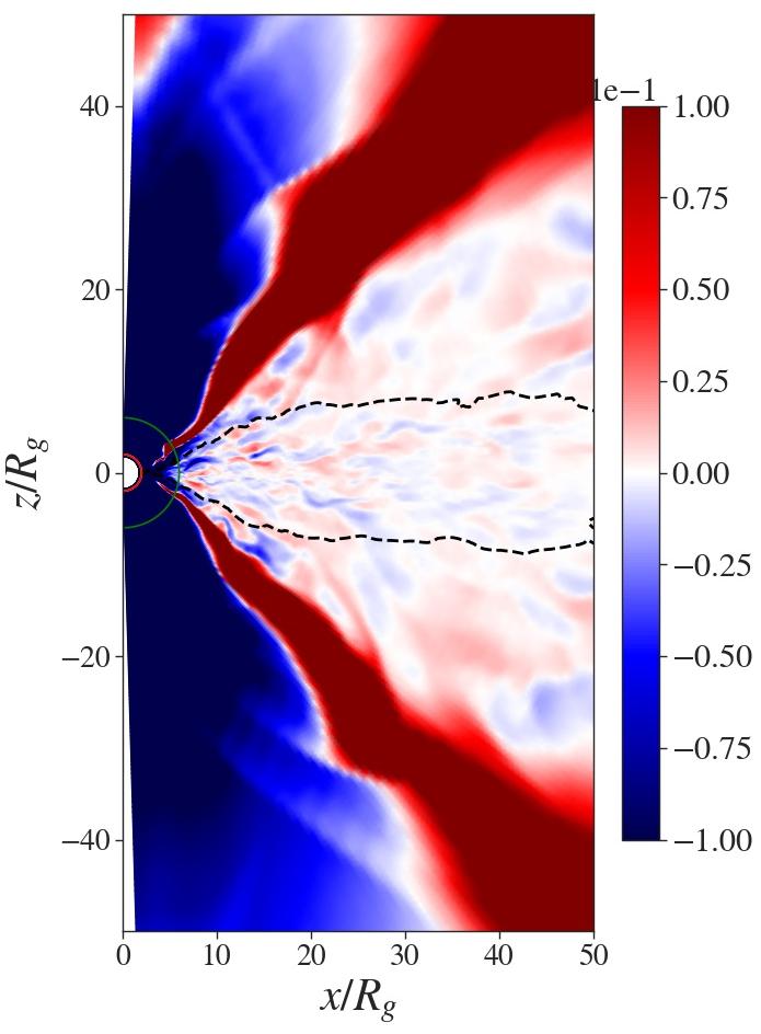
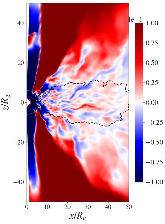
Figure 13: Radial velocity of the disk wind in the reference simulation sim1 at times $t=8000\text{ and }12000$. The black dashed line follows the density contour $\rho\approx 0.003$ which roughly indicates the size of disk and the transition to the coronal region.

However, we can still detect the launching of strong outflows. From our reference simulation sim1 (see Figure 7) we can see the evolution of small scale outflows from the disk surface which overall merge into a broad disk wind. The initially weak winds are launched by a combination of the increased magnetic field pressure gradient (mainly, but not only, from the toroidal component) and the re-arrangement of the accretion disk structure in the gravitational field of the black hole (advection of magnetic flux).

In Figure 13 we show the distribution of the radial velocity for the reference simulation at times $t=8000\text{ and }12000$. We also display the density contour $\rho\approx 0.003$ that could be understood as a proxy for the disk surface. A better choice would be transition from inflow to outflow, however, for most parts of the disk corona close to the disk, there is large-sized area with a constantly positive outwards velocity. Instead we find patches of both out-flowing and infalling material with velocities somewhat below $(<0.02c)$. This is the clear signature of a turbulent outflow structure. We note that here we are still dealing with the initial stages of outflow from the inner parts of the disk main body. Note that the magnetic field and the disk accretion is still evolving, as time $t=10000$ corresponds to only 50 inner disk orbits, much less than ones achieved in non-relativistic simulations.

An exception is a high-speed outflow that is rooted in the accretion funnel between the black hole and the ISCO. Here the gas into which the magnetic field is frozen-in orbits with high speed, resulting in radial outflow velocities up to $0.2c$.

In the last evolutionary stages the picture changes, however. The disk wind is now dominated by out-flowing patches moving with $\simeq 0.05c$. The infalling patches have almost disappeared and we see a substantial disk wind.

In the polar area above and below the black hole we see constant infall of material. Note this reference simulation is for a Schwarzschild black hole and no Blandford-Znajek-driving is possible (see below for rotating black holes). This axial area stays almost free of magnetic flux until the very final stages of the simulation. At this point in time, the accumulation of magnetic flux also leads to an increasing strength of the outflows from the inner part of the disk. These outflows are rooted in the accretion disk and outside the accretion funnel as they are seen in Figure 13.

Concerning the disk dynamics, we observe a mixture of positive and negative velocities, overall pointing towards a turbulent nature of the accretion disk. Strong accretion is only detected inside the marginally stable orbit.

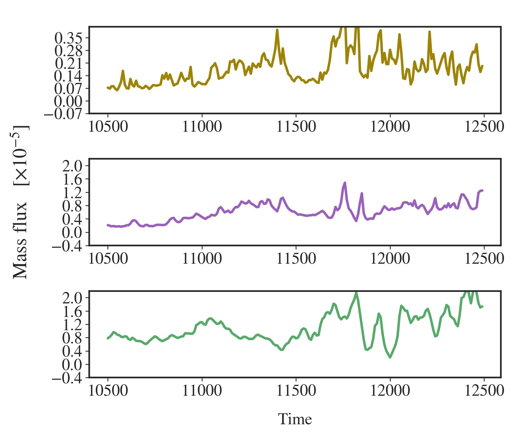
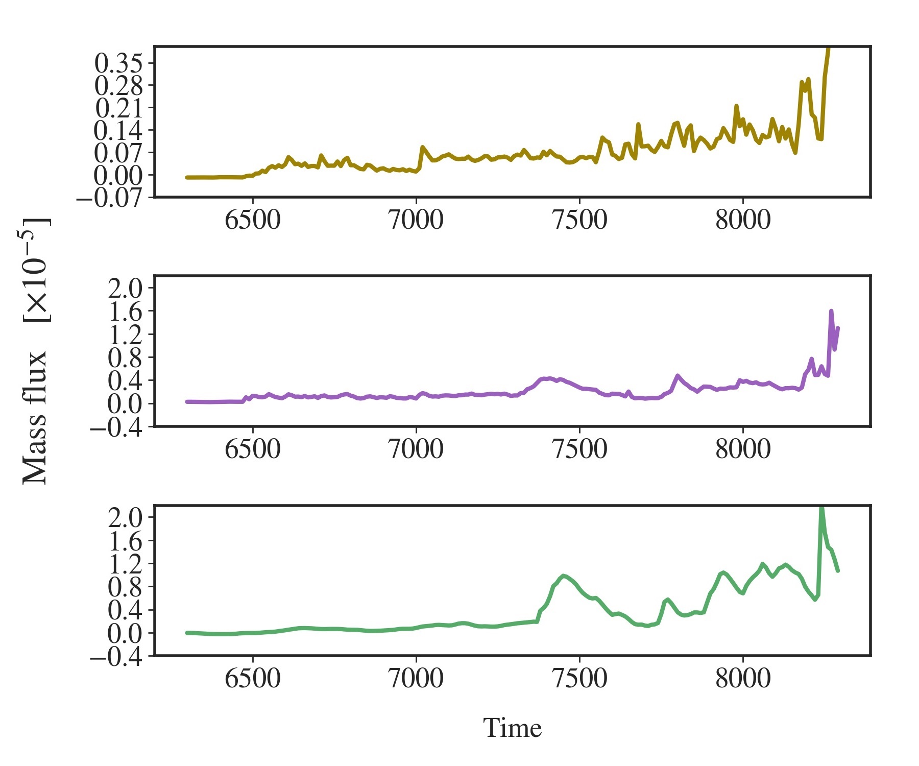
Figure 14: Integrated normalized radial mass flux through surfaces of constant radius at $r\sim 32$ for simulations sim0.1 (top) and sim1.1 (bottom). The integration is done along three different circular sections, between $0^{\circ}<\theta<25^{\circ}$, $25^{\circ}<\theta<65^{\circ}$, and $65^{\circ}<\theta<80^{\circ}$ including the symmetric sections in the lower hemisphere. Note the upper panels in the two groups of panels has tick marks almost an order of magnitude below the others.

Mow we want to quantify the fluxes carried by the outflows. In Figure 14 we show the (normalized) radial mass flux integrated along the polar angle at radius $r\sim 32$ for simulations sim0.1 and sim1.1. These values express the rate at which material is flowing outwards (positive values) or flowing inwards (accretion, collapse) towards the black hole (negative values).

We may compare three different regions along the polar angle. The first region is approximately $0^{\circ}<\theta<25^{\circ}$, which is the funnel region close to the rotational axis. The second region is within $25^{\circ}<\theta<65^{\circ}$ which represents the area where a high speed outflow may appear. The third region is within $65^{\circ}<\theta<80^{\circ}$, which is the area of a potential massive disk wind. The respective areas of the lower hemisphere are also added to the integration of the mass fluxes.

The figure only shows the evolution of the mass flux for the late times of the simulation, this is the time when a disk wind is established. When comparing the numerical values, we see that simulation sim0.1 shows stronger winds with an average mass flux in the second and third regions of $5.7\times 10^{-6}$ and $1.1\times 10^{-5}$. In contrast, in simulation sim1.1 we find mass fluxes that are only about 50% of that, namely $2.5\times 10^{-6}$, and $8.8\times 10^{-6}$, respectively.

Note that the only difference in these simulations is the threshold for the quenching (see Table 1). For sim1.1 the dynamo is quenched only at a higher magnetization level, therefore producing a correspondingly stronger flux (compare also to Figure 11). We learn from this comparison that an accretion disk that carries a stronger magnetic flux, will eventually generate an outflow of lower mass flux. We emphasize, however, that simulation sim1.1 terminates much earlier than simulation sim0.1 due to strong magnetic field close to the black hole. We suspect that if simulation sim1.1 would not have crashed, a correspondingly stronger wind would have been formed.

We close this section by noting that wind is strong enough to affect the disk mass evolution, thus changing the slope of the disk mass evolution towards a larger mass loss, i.e. a more rapidly decreasing disk mass (see Figure 9, bottom).

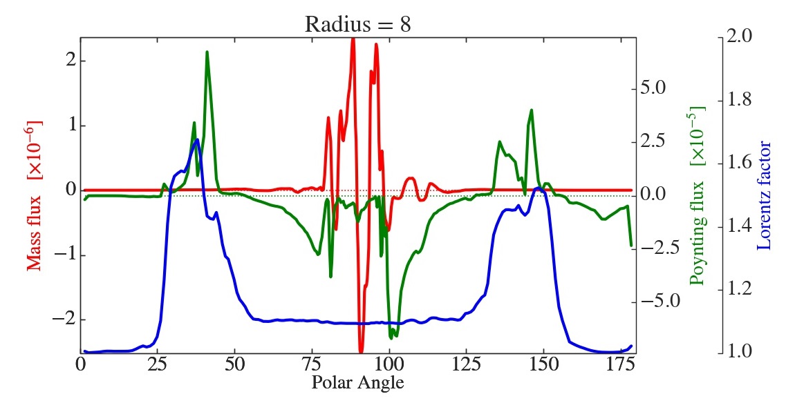
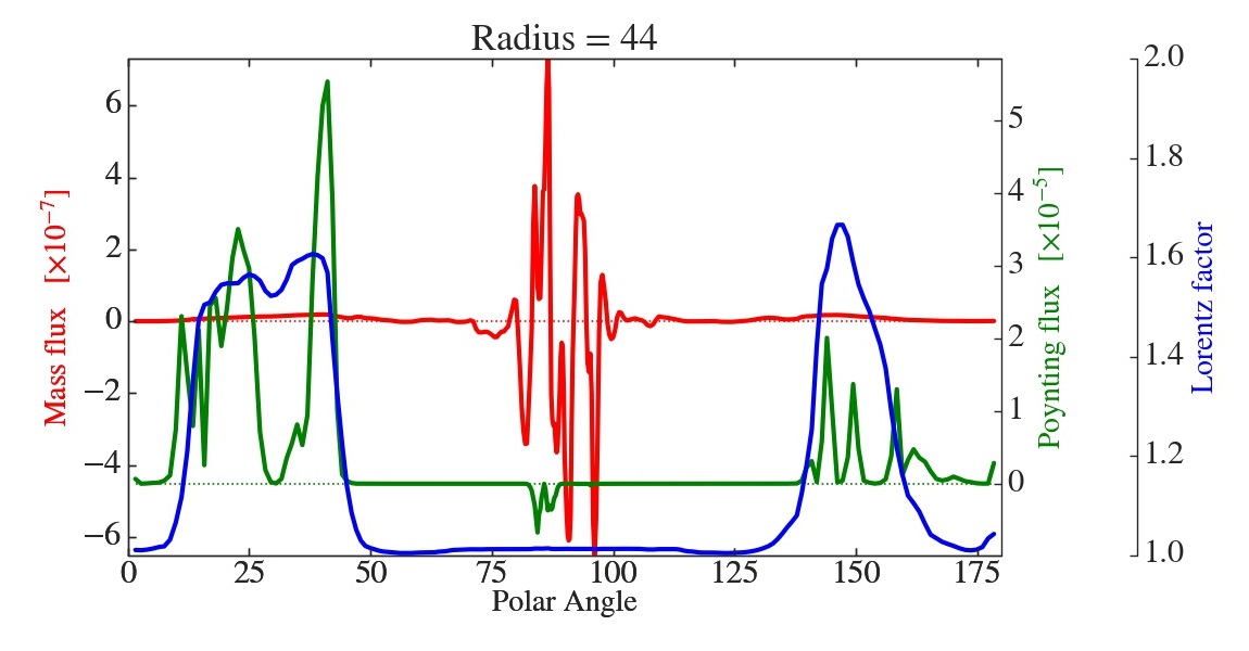
Figure 15: Comparison of the angular distribution of normalized mass flux (red), Poynting flux per solid angle (green) and Lorentz factor (blue) for simulation sim0.1 at $t=7000$ at radius $r=8$ and $r=44$ for both hemispheres. Negative mass flux indicates accretion towards the black hole. The Blandford-Znajek driven jet funnel is clearly distinguished by the peaks in Lorentz factor and electromagnetic energy flux. The mass flux increases with radius demonstrating a disk wind that is dominated by disk material.

5.5 Generating a Blandford-Znajek jet

Simulations with rotating black holes show the launching of strong outflows from the black hole magnetosphere, especially in later stages when the magnetic field has engulfed the axial area. This is a clear signature of Blandford-Znajek jets driven by the black hole ergosphere. In Figure 15 we show the angular profile of mass flux, Poynting flux and Lorentz factor at radii $r=8,44$ and at $t=7000$ for simulation sim0.1.

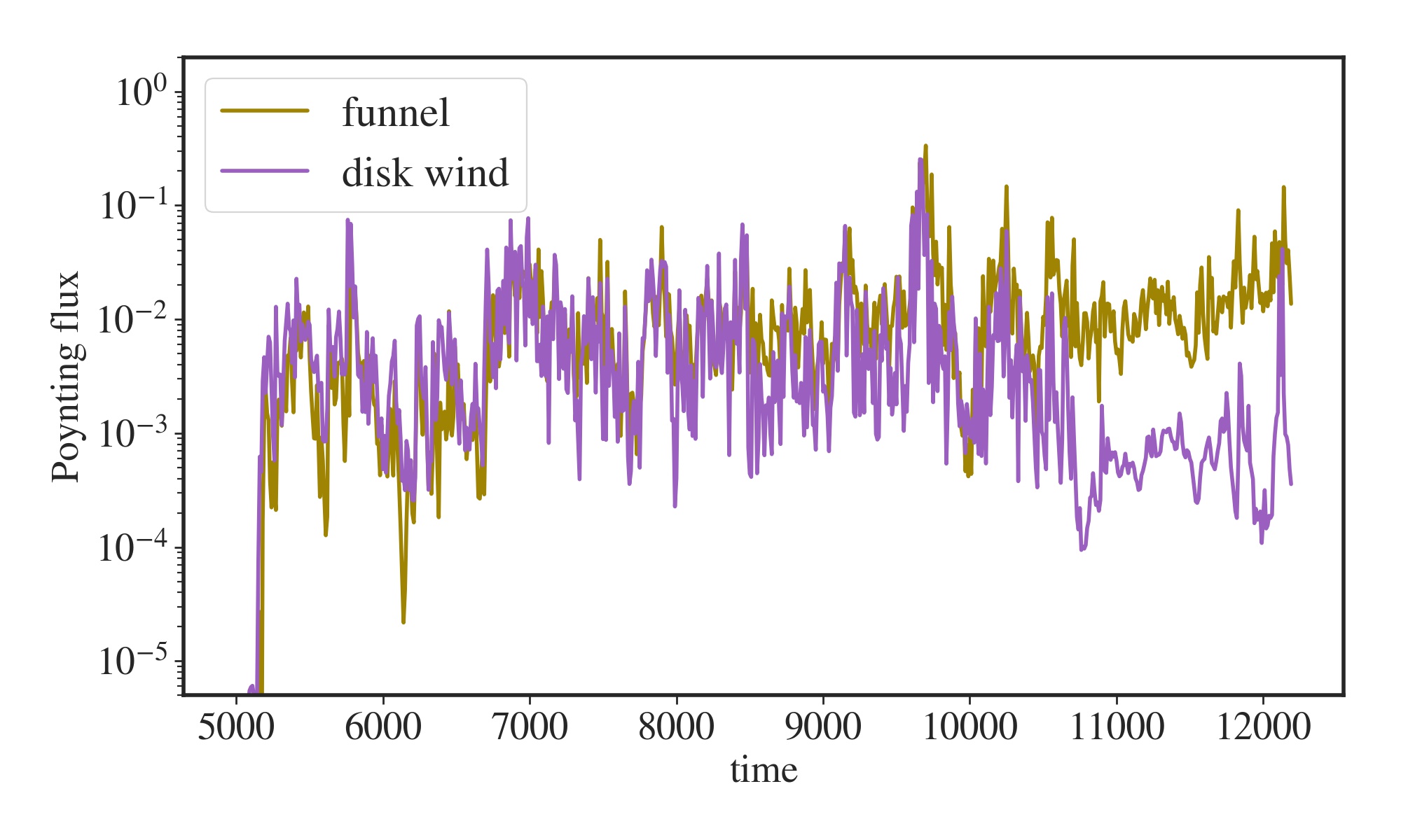
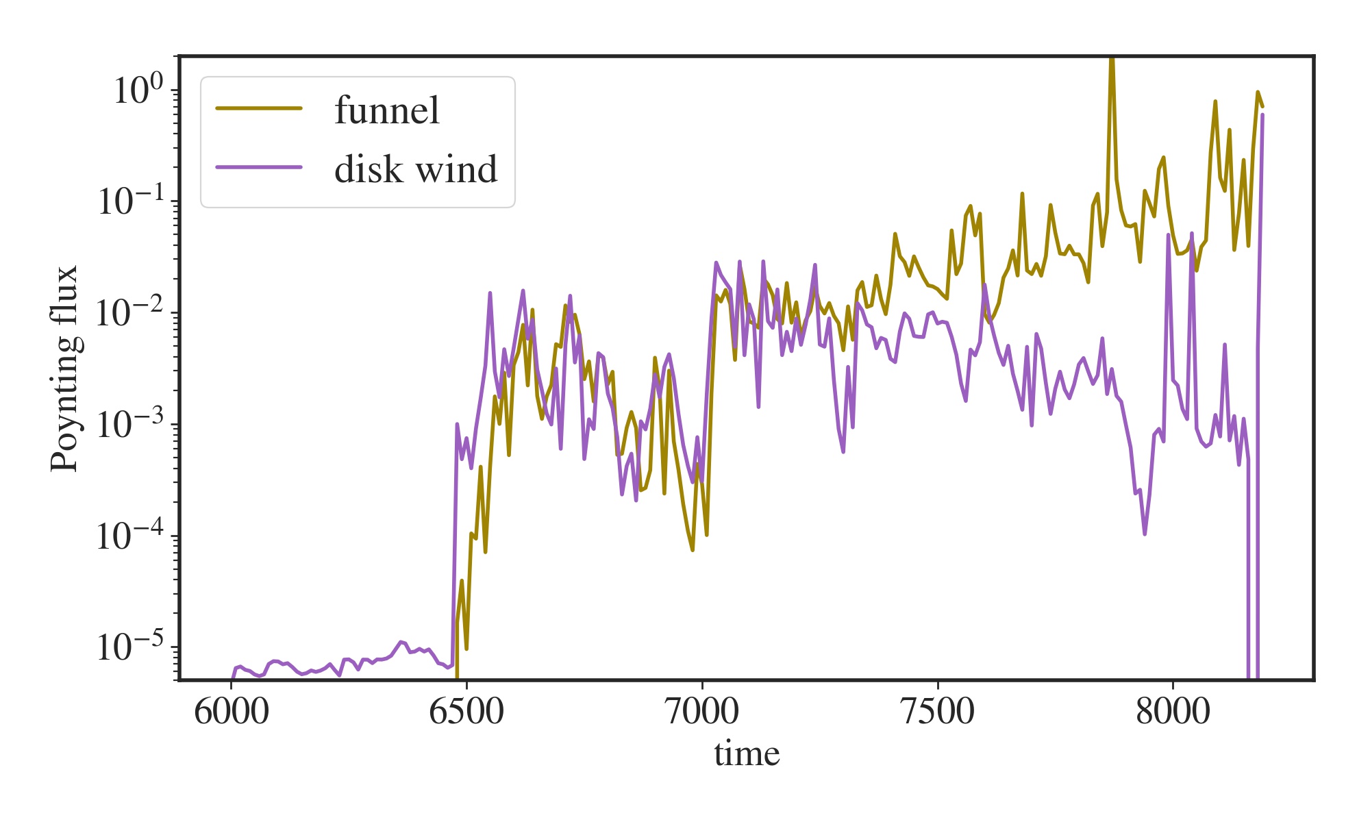
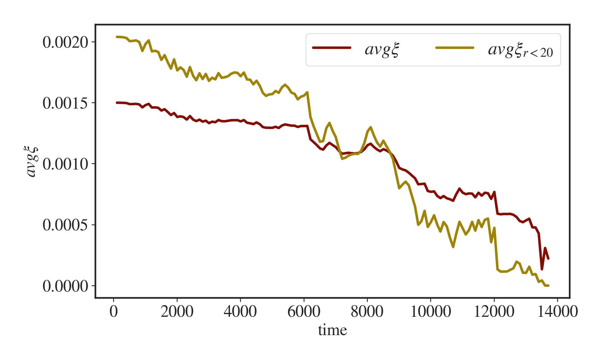
Figure 16: Integrated Poynting flux (top) through surfaces of constant radius $r\sim 32$ for simulations sim0.1 (left) and sim1.1 (right), respectively. The integration is done along two segments, between $0^{\circ}<\theta<25^{\circ}$ (funnel) and $25^{\circ}<\theta<65^{\circ}$ (disk wind), and their corresponding areas in the lower hemisphere, respectively. The corresponding evolution of the absolute dynamo parameter $\xi$ (bottom), averaged in space for the whole disk and the inner area $(r<20)$.

For the inner radius the mass flux has negative values around the equatorial plane which change into positive ones for slightly higher and lower angles. Accretion towards the black hole is determined by the negative mass flux, while the mass outflow in the radial direction is attributed to a low velocity wind from the inner disk and is expressed by the positive values. For angles closer to the polar axis the mass flux decreases significantly. In this area the mass flux is determined by the floor density chosen for the simulation, a feature that is common to all GRMHD simulations in the literature. Note however, that in our case only the axial outflow is affected and not the disk wind that is loaded with disk material and that carries a gas density is substantially higher than the floor values. The Poynting flux remains largely negative for polar angles close to the equatorial plane. It is positive for angles closer to the axis, indicative of a Poynting-dominated Blandford-Znajek jet. Similarly, this is accompanied by increasing Lorentz factor towards the axis, again implying the launching of a relativistic jet.

The picture becomes even more clear for the respective profiles derived for the larger radius. The Poynting flux is predominately positive in all directions with the higher values detected for the relativistic jet, similar for the Lorentz factor. Note that this Poynting flux is essentially generated by the disk dynamo and either launched directly from the disk surface, or, after advection of magnetic flux along the accretion disk, being further amplified by the black hole rotation.

The mass flux, however, gives a somewhat different picture. It shows variations across the equatorial plane with quite large positive and negative deviations from an average value (about more than 4 times lower than the variations in the inner disk). At this point in time, at radius $r=44$ the disk has completed almost 4 orbits around the black hole. This has to be compared to almost 45 disk orbits at $r=8$. The much slower evolution of the outer parts of the disk, in combination with the entangled magnetic field results in a much more turbulent accretion pattern of the outer disk parts. Reconnection also plays a role as the entangled magnetic field may be anti-aligned (see also Vourellis et al. (2019) for a discussion of resistive effects for GRMHD jet launching). Note however, that the evolutionary time of the outflow is quite faster than the disk evolution, meaning that the observed outflow dynamics provide an instant tracer of the launching conditions at the foot point of the outflow.

In Figure 16 we show the evolution of integrated Poynting flux (integrated along circles of constant radius, $r=32$) for simulations sim0.1 and sim1.1 hosted by a rotating black hole with $a=0.9$. We concentrate on two regions. One is the axial funnel area of $0^{\circ}<\theta<25^{\circ}$ where the relativistic jet launched by the black hole magnetosphere is propagating. The other is the disk wind area of $25^{\circ}<\theta<65^{\circ}$ where massive outflows from the disk are being launched. The values of the symmetric areas in the lower hemisphere are taken into account as well. We focus on the later stages of the simulations when the Poynting flux increases substantially.

The phase of strong Poynting flux begins approximately at the same time for both simulations. However, the higher threshold in plasma-$\beta$ for the dynamo quenching allows simulation sim0.1 to establish a high Poynting flux for a much longer time. In both simulations the Poynting flux measured in the jet funnel and in disk wind start with similar strength. Magnetic flux is advected and when the area close the black hole and the axial region is more and more encompassed by the dynamo-generated magnetic field, we see that the flux within the funnel increases while the flux of the disk wind decreases (see the diverging lines in Fig. 16, top panels). Our interpretation is that magnetic flux that is first anchored in the disk, is advected to the funnel, thus increasing the funnel flux and reducing the disk flux. Especially for simulation sim1.1 this reconfiguration process is more obvious. In Figure 16 (bottom) we show the evolution of the averaged absolute value of the disk dynamo parameter $\xi$ for the same two simulations. For simulation sim1.1, for which the quenching of the dynamo starts around $\beta_{eq}=100$, we notice the flat profile for the dynamo coincides with the absence of Poynting flux until the sudden increase of the Poynting flux. Later, when the flux from the disk wind decreases $(t\simeq 7250)$ we find a slight increase in the average dynamo parameter, especially for the one that includes the outer part of the disk.

These considerations are also supported by the time evolution of the magnetic flux of the disk and the black hole that we have discussed above (see Figure 11). From the poloidal flux advected to the ergosphere, the black hole rotation will induce a toroidal magnetic field, thus also increasing the Poynting flux. Note that at this point in time the dynamo action has been reduced significantly due to the quenching (see Section 5.3) and only little magnetic flux can be generated. Thus, the dynamo action is saturated and in balance with quenching.

6 Summary

In this paper, we have extended our resistive GRMHD code rHARM3D (Qian et al., 2017; Vourellis et al., 2019) implementing a mean- field dynamo in order to study the generation of a large-scale magnetic field and its effect on the launching of outflows. We have focused on a setup considering a thin accretion disk around a black holes running a number of simulation with various thresholds for the dynamo quenching and also applying different Kerr parameters for the black hole rotation.

Our mean-field dynamo simulations for thin accretion disk are initiated with a weak seed field in radial direction that is confined to the disk. The diffusivity profile follows a plateau profile within the disk and quickly drops across the disk surface towards an ideal MHD corona. Similarly, the profile for the mean-field dynamo parameter $\xi$ follows a sinusoidal profile in vertical direction from the the equatorial plane and a $1/\sqrt{r}$ profile along radius.

In the following we summarize our results.

(1) Our implementation of the mean-field dynamo is based on the work of Bucciantini & Del Zanna (2013) and is an extension of the purely resistive version of our code (Vourellis et al., 2019). The dynamo parameter $\xi$ (corresponding to the common dynamo-alpha in the literature) is inserted into Ohm’s law as a source of the magnetic field, and via the Maxwell’s equations into an equation for the evolution of the electric field. We also apply a quenching mechanism to mitigate the exponential increase of the magnetic field.

(2) We first set up a torus initial setup for the simulations. When comparing our results to those of Bugli et al. (2014); Tomei et al. (2020), we find in general good agreement in the sense that the dynamo produces similar field structures within the inner torus. In addition to the published literature we (i) continue the torus magnetic field evolution to longer times scales, thereby being able to follow the advection of magnetic flux towards the black hole rotational axis, and (ii) also provide the magnetic field lines of the field generated by the torus dynamo.

(3) The magnetic field evolution of the torus shows a saturation without applying a classical dynamo quenching for the $\alpha$-effect in the code as was reported by Tomei et al. (2020). We hypothesize that in this particular case the saturation of the dynamo process was established by reconnection of the dynamo-produced tangled magnetic field. We propose this as another channel of dynamo quenching that works self-consistently in a turbulent state of MHD, as long as physical resistivity is considered.

(4) Overall, the dynamo works as expected from non-relativistic simulations with the magnetic field lines emerging from the disk interior and expanding into the disk corona as the disk magnetic energy increases rapidly already at the beginning of the simulation. Dynamo action slows down mainly due to the quenching function we apply.

The poloidal magnetic field dominates over the toroidal component especially in the outer parts of the disk where the difference can be an order of magnitude. The outer parts of the disk remain weakly magnetized (at the time steps investigated), but the disk magnetization still slowly increases till the final simulation times, with the toroidal field component again dominating.

(5) We have also examined the evolution of the large-scale magnetic flux from the black hole-disk system for simulations applying different quenching levels for the dynamo as well as for rotating and non-rotating black holes, as the flux is an essential quantity for jet launching. The time evolution of the magnetic flux basically follows the evolution of magnetic energy and it is naturally affected by the quenching threshold. Even though the first stage is almost identical to all simulations, the ones with lower quenching threshold in plasma-$\beta$ increase their magnetic field faster in the later stages to the point that they also terminate faster. Black hole rotation appears to induce a delay in the increase of magnetic flux and also leads to the higher levels of magnetization.

(6) The hydrodynamic evolution of the disk changes with the growth of the magnetic field. Initially, the radial structure of the seed field allows for episodic accretion until the strong, dynamo generated field has evolved. The existence of a dynamo-generated, strong vertical field component allows for the gradual appearance of disk winds, which in turn lead to a smoothing of the otherwise quite peaky accretion rate. At the final stages of the simulations, the interplay between dynamo activity and dynamo quenching, together with the diffusion of magnetic flux, allows to develop a stronger disk wind together with a relativistic axial jet.

(7) We have identified small-scale disk outflows that are launched during the earlier stages of the simulations from the inner part of the accretion disk and which are interrelated with the presence of a strong magnetic field. These small-scale outflows maybe considered as disk flares. At the later stages of the simulation strong disk winds are ejected along the poloidal magnetic field, being mainly supported by the magnetic pressure of the toroidal field component. We do not find indication for Blandford-Payne driven disk winds in our setup and for the time scales considered, as the disk winds is kinematically dominated (as also in the found in the simulations by Vourellis et al. (2019).

(8) In our simulations considering rotating black holes, we observe an additional outflow structure that is a highly relativistic jet, apparently driven by the Blandford-Znajek mechanism. This jet carries a large electromagnetic energy flux when it leaves the ergosphere into the axial regions above the poles of the black hole (jet funnel). By measuring the Poynting flux both in the jet funnel and in the disk wind, we find that the flux in the jet funnel increases over time in expense of the magnetic flux in the disk wind. While the dynamo is quenched during later simulation times, and, thus, the disk magnetic flux becomes saturated, advection of magnetic flux along the disk towards the black hole leads to the high levels of Poynting flux we observe in the funnel.

In summary, we have applied, for the first time, the mean-field dynamo theory in the GRMHD context of thin accretion disks around black holes. We have investigated the evolution of the dynamo-generated magnetic field, the accretion disk and the outflows that are launched with the help of the evolved magnetic field. In particular we discuss the structure and evolution of the poloidal magnetic flux.

We find that the dynamo-generated magnetic field does not follow a clear dipolar structure, in difference to non-relativistic studies in the literature. Future work is needed to understand the mean-field dynamo action in GRMHD in more detail, in particular simulations running for longer time scales. The lack of a well-aligned, large scale dipolar field does not allow to launch strong disk winds via magneto-centrifugal driving. However, when the dynamo-generated magnetic field reaches a critical level, it is well capable to launch magnetic pressure driven disk winds and also highly relativistic jets from the black hole ergosphere.

References

- Abramowicz & Fragile (2013) Abramowicz, M. A., & Fragile, P. C. 2013, Living Reviews in Relativity, 16, 1, doi: 10.12942/lrr-2013-1
- Balbus & Hawley (1991) Balbus, S. A., & Hawley, J. F. 1991, ApJ, 376, 214, doi: 10.1086/170270
- Balbus & Hawley (1998) —. 1998, Reviews of Modern Physics, 70, 1, doi: 10.1103/RevModPhys.70.1
- Bardou et al. (2001) Bardou, A., von Rekowski, B., Dobler, W., Brand enburg, A., & Shukurov, A. 2001, Astronomy and Astrophysics, 370, 635, doi: 10.1051/0004-6361:20010267
- Blackman & Field (1993) Blackman, E. G., & Field, G. B. 1993, Phys. Rev. Lett., 71, 3481, doi: 10.1103/PhysRevLett.71.3481
- Blandford & Payne (1982) Blandford, R. D., & Payne, D. G. 1982, MNRAS, 199, 883, doi: 10.1093/mnras/199.4.883
- Blandford & Znajek (1977) Blandford, R. D., & Znajek, R. L. 1977, MNRAS, 179, 433, doi: 10.1093/mnras/179.3.433
- Brandenburg (1996) Brandenburg, A. 1996, ApJ, 465, L115, doi: 10.1086/310142
- Brandenburg et al. (1995) Brandenburg, A., Nordlund, A., Stein, R. F., & Torkelsson, U. 1995, ApJ, 446, 741, doi: 10.1086/175831
- Bucciantini & Del Zanna (2011) Bucciantini, N., & Del Zanna, L. 2011, Astronomy and Astrophysics, 528, A101, doi: 10.1051/0004-6361/201015945
- Bucciantini & Del Zanna (2013) —. 2013, MNRAS, 428, 71, doi: 10.1093/mnras/sts005
- Bugli et al. (2014) Bugli, M., Del Zanna, L., & Bucciantini, N. 2014, MNRAS, 440, L41, doi: 10.1093/mnrasl/slu017
- Bugli et al. (2018) Bugli, M., Guilet, J., Müller, E., et al. 2018, MNRAS, 475, 108, doi: 10.1093/mnras/stx3158
- Casse & Keppens (2002) Casse, F., & Keppens, R. 2002, ApJ, 581, 988, doi: 10.1086/344340
- Cattaneo & Tobias (2014) Cattaneo, F., & Tobias, S. M. 2014, ApJ, 789, 70, doi: 10.1088/0004-637X/789/1/70
- Cerdá-Durán et al. (2007) Cerdá-Durán, P., Font, J. A., & Dimmelmeier, H. 2007, A&A, 474, 169, doi: 10.1051/0004-6361:20077432
- De Villiers & Hawley (2003) De Villiers, J.-P., & Hawley, J. F. 2003, ApJ, 589, 458, doi: 10.1086/373949
- Del Zanna et al. (2007) Del Zanna, L., Zanotti, O., Bucciantini, N., & Londrillo, P. 2007, A&A, 473, 11, doi: 10.1051/0004-6361:20077093
- Dyda et al. (2018) Dyda, S., Lovelace, R. V. E., Ustyugova, G. V., Koldoba, A. V., & Wasserman, I. 2018, MNRAS, 477, 127, doi: 10.1093/mnras/sty614
- Fendt (1997) Fendt, C. 1997, A&A, 319, 1025
- Fendt & Gaßmann (2018) Fendt, C., & Gaßmann, D. 2018, The Astrophysical Journal, 855, 130, doi: 10.3847/1538-4357/aab14c
- Fendt & Greiner (2001) Fendt, C., & Greiner, J. 2001, A&A, 369, 308, doi: 10.1051/0004-6361:20010108
- Ferreira (1997) Ferreira, J. 1997, A&A, 319, 340
- Fishbone & Moncrief (1976) Fishbone, L. G., & Moncrief, V. 1976, ApJ, 207, 962, doi: 10.1086/154565
- Fleming et al. (2000) Fleming, T. P., Stone, J. M., & Hawley, J. F. 2000, ApJ, 530, 464, doi: 10.1086/308338
- Gammie et al. (2003) Gammie, C. F., McKinney, J. C., & Tóth, G. 2003, ApJ, 589, 444, doi: 10.1086/374594
- Ghosh (2000) Ghosh, P. 2000, MNRAS, 315, 89, doi: 10.1046/j.1365-8711.2000.03410.x
- Giesecke et al. (2005) Giesecke, A., Rüdiger, G., & Elstner, D. 2005, Astronomische Nachrichten, 326, 693, doi: 10.1002/asna.200510405
- Gressel (2010) Gressel, O. 2010, MNRAS, 405, 41, doi: 10.1111/j.1365-2966.2010.16440.x
- Gressel & Pessah (2015) Gressel, O., & Pessah, M. E. 2015, ApJ, 810, 59, doi: 10.1088/0004-637X/810/1/59
- Hughes & Tobias (2010) Hughes, D. W., & Tobias, S. M. 2010, An Introduction to Mean Field Dynamo Theory, 15–48, doi: 10.1142/9789814291552_0002
- Khanna & Camenzind (1996a) Khanna, R., & Camenzind, M. 1996a, A&A, 307, 665
- Khanna & Camenzind (1996b) —. 1996b, A&A, 313, 1028
- Koide et al. (1999) Koide, S., Shibata, K., & Kudoh, T. 1999, ApJ, 522, 727, doi: 10.1086/307667
- Komissarov (2005) Komissarov, S. S. 2005, MNRAS, 359, 801, doi: 10.1111/j.1365-2966.2005.08974.x
- Komissarov (2007) —. 2007, MNRAS, 382, 995, doi: 10.1111/j.1365-2966.2007.12448.x
- Küker & Rüdiger (1999) Küker, M., & Rüdiger, G. 1999, A&A, 346, 922
- Longaretti & Lesur (2010) Longaretti, P.-Y., & Lesur, G. 2010, A&A, 516, A51, doi: 10.1051/0004-6361/201014093
- Lynden-Bell (1996) Lynden-Bell, D. 1996, MNRAS, 279, 389, doi: 10.1093/mnras/279.2.389
- Mahlmann et al. (2018) Mahlmann, J. F., Cerdá-Durán, P., & Aloy, M. A. 2018, MNRAS, 477, 3927, doi: 10.1093/mnras/sty858
- Matsumoto et al. (2020) Matsumoto, J., Takiwaki, T., Kotake, K., Asahina, Y., & Takahashi, H. R. 2020, MNRAS, 499, 4174, doi: 10.1093/mnras/staa3095
- Mattia & Fendt (2020) Mattia, G., & Fendt, C. 2020, ApJ, submitted
- Misner et al. (1973) Misner, C. W., Thorne, K. S., & Wheeler, J. A. 1973, Gravitation
- Moffatt (1978) Moffatt, H. K. 1978, Magnetic field generation in electrically conducting fluids
- Murphy et al. (2010) Murphy, G. C., Ferreira, J., & Zanni, C. 2010, A&A, 512, A82, doi: 10.1051/0004-6361/200912633
- Nigro et al. (2017) Nigro, G., Pongkitiwanichakul, P., Cattaneo, F., & Tobias, S. M. 2017, MNRAS, 464, L119, doi: 10.1093/mnrasl/slw190
- Noble et al. (2006) Noble, S. C., Gammie, C. F., McKinney, J. C., & Del Zanna, L. 2006, ApJ, 641, 626, doi: 10.1086/500349
- Obergaulinger et al. (2018) Obergaulinger, M., Just, O., & Aloy, M. A. 2018, Journal of Physics G Nuclear Physics, 45, 084001, doi: 10.1088/1361-6471/aac982
- Paczyńsky & Wiita (1980) Paczyńsky, B., & Wiita, P. J. 1980, A&A, 88, 23
- Pan et al. (2017) Pan, Z., Yu, C., & Huang, L. 2017, ApJ, 836, 193, doi: 10.3847/1538-4357/aa5c36
- Pariev et al. (2007) Pariev, V. I., Colgate, S. A., & Finn, J. M. 2007, The Astrophysical Journal, 658, 129, doi: 10.1086/510735
- Parker (1955) Parker, E. N. 1955, ApJ, 122, 293, doi: 10.1086/146087
- Porth et al. (2017) Porth, O., Olivares, H., Mizuno, Y., et al. 2017, Computational Astrophysics and Cosmology, 4, 1, doi: 10.1186/s40668-017-0020-2
- Pu & Takahashi (2020) Pu, H.-Y., & Takahashi, M. 2020, ApJ, 892, 37, doi: 10.3847/1538-4357/ab77ab
- Pudritz (1981a) Pudritz, R. E. 1981a, MNRAS, 195, 881, doi: 10.1093/mnras/195.4.881
- Pudritz (1981b) —. 1981b, MNRAS, 195, 897, doi: 10.1093/mnras/195.4.897
- Pudritz & Norman (1986) Pudritz, R. E., & Norman, C. A. 1986, ApJ, 301, 571, doi: 10.1086/163924
- Qian et al. (2017) Qian, Q., Fendt, C., Noble, S., & Bugli, M. 2017, ApJ, 834, 29, doi: 10.3847/1538-4357/834/1/29
- Qian et al. (2018) Qian, Q., Fendt, C., & Vourellis, C. 2018, ApJ, 859, 28, doi: 10.3847/1538-4357/aabd36
- Rieger (2019) Rieger, F. M. 2019, Galaxies, 7, 78, doi: 10.3390/galaxies7030078
- Ripperda et al. (2019) Ripperda, B., Bacchini, F., Porth, O., et al. 2019, ApJS, 244, 10, doi: 10.3847/1538-4365/ab3922
- Ruediger et al. (1995) Ruediger, G., Elstner, D., & Stepinski, T. F. 1995, A&A, 298, 934
- Sheikhnezami et al. (2012) Sheikhnezami, S., Fendt, C., Porth, O., Vaidya, B., & Ghanbari, J. 2012, ApJ, 757, 65, doi: 10.1088/0004-637X/757/1/65
- Sądowski et al. (2015) Sądowski, A., Narayan, R., Tchekhovskoy, A., et al. 2015, MNRAS, 447, 49, doi: 10.1093/mnras/stu2387
- Steenbeck & Krause (1969a) Steenbeck, M., & Krause, F. 1969a, Astronomische Nachrichten, 291, 49, doi: 10.1002/asna.19692910201
- Steenbeck & Krause (1969b) —. 1969b, Astronomische Nachrichten, 291, 271
- Stepanovs & Fendt (2014) Stepanovs, D., & Fendt, C. 2014, ApJ, 793, 31, doi: 10.1088/0004-637X/793/1/31
- Stepanovs & Fendt (2016) —. 2016, ApJ, 825, 14, doi: 10.3847/0004-637X/825/1/14
- Stepanovs et al. (2014) Stepanovs, D., Fendt, C., & Sheikhnezami, S. 2014, ApJ, 796, 29, doi: 10.1088/0004-637X/796/1/29
- Stone et al. (1996) Stone, J. M., Hawley, J. F., Gammie, C. F., & Balbus, S. A. 1996, ApJ, 463, 656, doi: 10.1086/177280
- Takahashi et al. (2018) Takahashi, K., Toma, K., Kino, M., Nakamura, M., & Hada, K. 2018, ApJ, 868, 82, doi: 10.3847/1538-4357/aae832
- Tomei et al. (2020) Tomei, N., Del Zanna, L., Bugli, M., & Bucciantini, N. 2020, MNRAS, 491, 2346, doi: 10.1093/mnras/stz3146
- Tomimatsu & Takahashi (2003) Tomimatsu, A., & Takahashi, M. 2003, ApJ, 592, 321, doi: 10.1086/375579
- Uchida & Shibata (1985) Uchida, Y., & Shibata, K. 1985, PASJ, 37, 515
- Vlahakis & Königl (2001) Vlahakis, N., & Königl, A. 2001, ApJ, 563, L129, doi: 10.1086/338652
- von Rekowski & Brandenburg (2004) von Rekowski, B., & Brandenburg, A. 2004, Astronomy and Astrophysics, 420, 17, doi: 10.1051/0004-6361:20034065
- von Rekowski et al. (2003) von Rekowski, B., Brandenburg, A., Dobler, W., Dobler, W., & Shukurov, A. 2003, Astronomy and Astrophysics, 398, 825, doi: 10.1051/0004-6361:20021699
- Vourellis et al. (2019) Vourellis, C., Fendt, C., Qian, Q., & Noble, S. C. 2019, ApJ, 882, 2, doi: 10.3847/1538-4357/ab32e2
- Wald (1974) Wald, R. M. 1974, Phys. Rev. D, 10, 1680, doi: 10.1103/PhysRevD.10.1680
- Weiss et al. (1984) Weiss, N. O., Cattaneo, F., & Jones, C. A. 1984, Geophysical and Astrophysical Fluid Dynamics, 30, 305, doi: 10.1080/03091928408219262
- Zanni et al. (2007) Zanni, C., Ferrari, A., Rosner, R., Bodo, G., & Massaglia, S. 2007, A&A, 469, 811, doi: 10.1051/0004-6361:20066400