Cosmic variance of H0subscript𝐻0H_{0} in light of forthcoming high-redshift surveys

Giuseppe Fanizza1 gfanizza@fc.ul.pt    Bartolomeo Fiorini2 bartolomeo.fiorini@port.ac.uk    Giovanni Marozzi3,4 giovanni.marozzi@unipi.it 1Instituto de Astrofisíca e Ciências do Espaço, Faculdade de Ciências da Universidade de Lisboa, Edificio C8, Campo Grande, P-1740-016, Lisbon, Portugal 2Institute of Cosmology & Gravitation, University of Portsmouth, Dennis Sciama Building, Burnaby Road, Portsmouth, PO1 3FX United Kingdom 3Dipartimento di Fisica, Università di Pisa, Largo B. Pontecorvo 3, 56127 Pisa, Italy 4Istituto Nazionale di Fisica Nucleare, Sezione di Pisa, Pisa, Italy
Abstract

Forthcoming surveys will extend the understanding of cosmological large scale structures up to unprecedented redshift. According to this perspective, we present a fully relativistic framework to evaluate the impact of stochastic inhomogeneities on the determination of the Hubble constant. To this aim, we work within linear perturbation theory and relate the fluctuations of the luminosity distance-redshift relation, in the Cosmic Concordance model, to the intrinsic uncertainty associated to the measurement of H0subscript𝐻0H_{0} from high-redshift surveys (0.15z3.850.15𝑧3.850.15\leq z\leq 3.85). We first present the detailed derivation of the luminosity distance-redshift relation 2-point correlation function and then provide analytical results for all the involved relativistic effects, such as peculiar velocity, lensing, time delay and (integrated) Sachs-Wolfe, and their angular spectra. Hence, we apply our analytical results to the study of high-redshift Hubble diagram, according to what has been recently claimed in literature. Following the specific of Euclid Deep Survey and LSST, we conclude that the cosmic variance associated with the measurement of the Hubble constant is at most of 0.1 %. Our work extends the analysis already done in literature for closer sources, where only peculiar velocity has been taken into account. We then conclude that deep surveys will provide an estimation of the H0subscript𝐻0H_{0} which will be more precise than the one obtained from local sources, at least in regard of the intrinsic uncertainty related to a stochastic distribution of inhomogeneities.

pacs:
Valid PACS appear here

Introduction

The last 30 years have witnessed the evolution of cosmology from an order of magnitude description of the Universe into an area of the hard sciences where precision measurements are achievable. This change has its cornerstone in the estimation of cosmological parameters through the detection of Cosmic Microwave Background (CMB) spectra which provide so far the most precise measurements of these parameters. Given this astonishing success, forthcoming missions aim to push forward this result in order to infer measurements of cosmological parameters also from late-time dataset, such as Large Scale Structure (LSS) surveys (see, for example, Euclid Laureijs et al. (2011) and Vera C. Rubin Observatory Legacy Survey of Space and Time (LSST) Abell et al. (2009)) and Intensity Mapping (IM) (for instance, SKA Mellema et al. (2013) and HERA DeBoer et al. (2017)). One of the common goals shared within the community is to study late time probes in order to estimate cosmological parameters at a comparable level of precision with respect to the one achieved from CMB dataset. This program is highly motivated by several reasons. To mention a few, late time surveys provide 3-dimensional catalogs about the observed Universe, hence they may help understanding the evolution of the Universe rather than just giving a picture of it, as 2-dimensional datasets (CMB indeed) do111Here we underline that non-linearities in CMB lensing due to the bispectrum of the gravitational potential might turn CMB spectra into 3 dimensional datasets as well Marozzi et al. (2016, 2017, 2018); Di Dio et al. (2019).. Secondly, the non-linear evolution of the structures gets enhanced at later times. As a consequence, this allows to explore better non-linear scales in the distribution of matter in the Universe, distribution that contains useful information about the energy content of the Universe itself (for instance dark matter candidates and massive neutrinos). Last but not least, the measurements of late time probes furnish estimations for the cosmological parameters which are (almost) independent of the adopted model, differently from the CMB ones.

For what concerns the comparison between different reconstructions of cosmological parameters, last years have shown a discrepancy between the estimation of the present Hubble rate H0subscript𝐻0H_{0} from CMB and late time probes. Indeed, CMB measurements provide a value for H0=67.36±0.54subscript𝐻0plus-or-minus67.360.54H_{0}=67.36\pm 0.54 km s-1 Mpc-1 Aghanim et al. (2020), whereas late time estimations based on local probes, such as Supernovae Ia (SnIa), returns H0=73.2±1.3subscript𝐻0plus-or-minus73.21.3H_{0}=73.2\pm 1.3 km s-1 Mpc-1 Riess et al. (2021) (see Freedman et al. (2019, 2020); Wong et al. (2019); Yuan et al. (2019); Pesce et al. (2020) for other estimations): a discrepancy of almost 5σ5𝜎5\sigma emerges. A priori, both measurements might be questionable because of the following reasons. CMB estimation provides nowadays the most precise measurement of H0subscript𝐻0H_{0} but, to this end, requires (as mentioned) that a cosmological model is chosen in order to analyze the spectra. On the other hand, SnIa catalogs for close sources do not need any cosmological model to infer H0subscript𝐻0H_{0} but require to calibrate the relative magnitude of the observed standard candles wrt some sources whose luminosity is known (for instance the Cepheid host).

This tension seems to survive also when different late time probes are investigated Verde et al. (2019). This has raised the interest of the community into the following question: is there any need for new unknown physics to cancel (or at least mild) this discrepancy? In this regard, it might be that the sound horizon scale rssubscript𝑟𝑠r_{s} could be lower than the one predicted by our current knowledge of pre-recombination physics in the framework of ΛΛ\LambdaCDM model Bernal et al. (2016). In fact, since the acoustic angular peak measured by the CMB is proportional to rsH0subscript𝑟𝑠subscript𝐻0r_{s}H_{0}, this would automatically raise the value of H0subscript𝐻0H_{0} detected from the CMB towards the one inferred from local measurements. However, as discussed in Jedamzik et al. (2021), the modification of rssubscript𝑟𝑠r_{s} might be not enough to completely reabsorb the tension. In general, the search for new physics which could explain the discrepancy questions several aspects of the current Cosmic Concordance model. In particular, in Beenakker and Venhoek (2021) a set of 7 key assumptions which might be broken to explain the tension has been identified. All these reasons have motivated an intense research activity during the last years (see Knox and Millea (2020); Di Valentino et al. (2021) for overviews, and Di Valentino et al. (2016, 2017); Vagnozzi (2020); Ballardini et al. (2020); Ye et al. (2021), and references therein, for a partial coverage of the related literature). We mention also that a very interesting attempt to measure H0subscript𝐻0H_{0} from CMB lensing, without invoking the knowledge of rssubscript𝑟𝑠r_{s}, has been done in Baxter and Sherwin (2020). This method returns a rssubscript𝑟𝑠r_{s}-independent constraint of H0=73.5±5.3subscript𝐻0plus-or-minus73.55.3H_{0}=73.5\pm 5.3 km s-1 Mpc-1, which seems to reabsorb the tension.

Given this state-of-art, we will adopt an agnostic approach to the problem. Indeed, within the conservative framework of ΛΛ\LambdaCDM model222See Perivolaropoulos and Skara (2021) for a detailed review about the new challenges for ΛΛ\LambdaCDM., the question we aim to answer is the following: in view of the forthcoming LSS surveys, is there any theoretical bias which might increase the standard deviation in order to alleviate the tension? This question has already been partially faced in the past. In particular, in Ben-Dayan et al. (2014) the effect of velocity dispersion of local SnIa (at redshift lower than 0.1) has been studied and it has been shown that it can introduce a further intrinsic error in the local estimation of H0subscript𝐻0H_{0} of 1%similar-toabsentpercent1\sim 1\%. However, this effect can mitigate but not resolve the tension. In this work, we extend our analysis to forecast the estimated precision for catalog which will have deeper extension in redshift (up to redshift 3.85), just like Euclid Deep Survey (EDS) and LSST. To this aim, we will assume that the new generation of standard candles known as Superluminous Supernovae (SLSNe) will provide a suitable dataset for the analysis, following what has been recently claimed in Inserra et al. (2021). In the same spirit but concerning the forecast for future CMB surveys (such as CMB-S4 Abazajian et al. (2019)), in Baxter and Sherwin (2020) the forecasted error for the above-mentioned rssubscript𝑟𝑠r_{s}-independent measurement of H0subscript𝐻0H_{0} is about σH0=3subscript𝜎subscript𝐻03\sigma_{H_{0}}=3 km s-1 Mpc-1.

To perform the analysis, our starting point is to derive the analytical formula for the 2-point correlation function of the luminosity distance-redshift relation. Hence, we will discuss general aspects of this function, whose interests go beyond the ones concerning H0subscript𝐻0H_{0}. In particular, we will investigate numerically the cosmological information encrypted in the lowest angular multipoles of the 2-point correlation functions. To conclude, we will finalize our analysis by providing forecasted errors of 0.1%similar-toabsentpercent0.1\sim 0.1\% for EDS and 0.01%similar-toabsentpercent0.01\sim 0.01\% for LSST in regard of the measurement of H0subscript𝐻0H_{0}. These results are obtained by using linear power spectrum. However, as we will show, non-linear scales do not dramatically change this scenario. Their contribution enhances the forecasted errors to 0.1%similar-toabsentpercent0.1\sim 0.1\% for both EDS and LSST. This renders the measurement for high-redshift standard candles ideally much more precise than the one so far discussed in Ben-Dayan et al. (2014) for close sources.

The paper is organized as follows. In Sect. I we describe the general method followed to infer the value of H0subscript𝐻0H_{0}, from higher LSS surveys, thanks to the knowledge of the linear luminosity distance-redshift relation. In Sect. II we compute in details the 2-point correlation function for all the relativistic effects involved in the linear luminosity distance-redshift relation, providing general expressions for them. In Sect. III, we further give numerical details about the spectrum of lower angular multipoles for lensing and doppler effect, and a general treatment about the monopole concerning all the effects. In Sect. IV, we assume a numerical set of the cosmological parameters within the ΛΛ\LambdaCDM model and estimate the 2-point correlation function effect by effect. Furthermore, we discuss some technical approximations which speed up the numerical evaluations of the lensing effect. In Sect. V we outline the consequences of our numerical analysis according to the specifics of EDS and LSST and discuss the impact of non-linear scales. Finally, in Sect. VI we summarize our main conclusions. Moreover, in App. A we furnish technical details about the calculations of the 2-point correlation function. In App. B, we report explicit expression for the lower multipoles of the lensing angular spectrum. App. C contains useful properties of the spherical Bessel functions, whereas App. D contains details about the multipole expansion of lensing 2-point correlation function.

I Cosmic variance

The starting point for our analysis is the well-known expression for the luminosity distance-redshift relation dL(z)subscript𝑑𝐿𝑧d_{L}(z) in the homogenous and isotropic Cosmic Concordance model

dL(z)=1+zH00zdzΩ0m(1+z)3+Ω0Λ,subscript𝑑𝐿𝑧1𝑧subscript𝐻0superscriptsubscript0𝑧𝑑superscript𝑧subscriptΩ0𝑚superscript1superscript𝑧3subscriptΩ0Λd_{L}(z)=\frac{1+z}{H_{0}}\int_{0}^{z}\frac{dz^{\prime}}{\sqrt{\Omega_{0m}(1+z^{\prime})^{3}+\Omega_{0\Lambda}}}, (1)

where H0subscript𝐻0H_{0} is indeed the Hubble constant and Ω0msubscriptΩ0𝑚\Omega_{0m} and Ω0ΛsubscriptΩ0Λ\Omega_{0\Lambda} are respectively the energy density for the Cold Matter and Cosmological Constant today. Within the ΛΛ\LambdaCDM model assumptions, it is well known that Ω0Λ=1Ω0msubscriptΩ0Λ1subscriptΩ0𝑚\Omega_{0\Lambda}=1-\Omega_{0m} such that Eq. (1) contains only two free parameters. Eq. (1) can then be inverted and provides a relation which can be used to infer the value of H0subscript𝐻0H_{0} as

H0=1+zdL(z)0zdzΩ0m(1+z)3+1Ω0m.subscript𝐻01𝑧subscript𝑑𝐿𝑧superscriptsubscript0𝑧𝑑superscript𝑧subscriptΩ0𝑚superscript1superscript𝑧31subscriptΩ0𝑚H_{0}=\frac{1+z}{d_{L}(z)}\int_{0}^{z}\frac{dz^{\prime}}{\sqrt{\Omega_{0m}(1+z^{\prime})^{3}+1-\Omega_{0m}}}\,. (2)

In this way, given an a priori knowledge of Ω0msubscriptΩ0𝑚\Omega_{0m}, independent estimations for redshift and luminosity distance from a given sample of sources can provide a measurement of H0subscript𝐻0H_{0}.

Within this framework, the question that we want to address is then the following: how precise can in principle be this estimation if we consider the inhomogeneities all around our observed Universe? In other words, the observed luminosity distance-redshift relation dL(z)subscript𝑑𝐿𝑧d_{L}(z) is affected by the inhomogeneities and this provides an intrinsic dispersion for dL(z)subscript𝑑𝐿𝑧d_{L}(z) which is governed by the way the cosmological structures are distributed and evolve. Hence, in this regard, we consider the observed inhomogeneous luminosity distance-redshift relation dL~(z)~subscript𝑑𝐿𝑧\widetilde{d_{L}}(z)

dL~(z,𝐧)=dL(z)[1+δ(1)(z,𝐧)+δ(2)(z,𝐧)],~subscript𝑑𝐿𝑧𝐧subscript𝑑𝐿𝑧delimited-[]1superscript𝛿1𝑧𝐧superscript𝛿2𝑧𝐧\widetilde{d_{L}}(z,{\bf n})=d_{L}(z)\left[1+\delta^{(1)}(z,{\bf n})+\delta^{(2)}(z,{\bf n})\right]\,, (3)

where 𝐧𝐧{\bf n} is the observed direction for the given source and δ(1)superscript𝛿1\delta^{(1)} and δ(2)superscript𝛿2\delta^{(2)} are linear and second order corrections to the luminosity distance-redshift relation. Let us underline that here we do not have to consider perturbations in the redshift z𝑧z. Indeed, the inhomogeneous dL~(z)~subscript𝑑𝐿𝑧\widetilde{d_{L}}(z) is evaluated by construction at constant observed redshift hypersurfaces. This means that redshift corrections are already taken into account in the dL~(z,𝐧)~subscript𝑑𝐿𝑧𝐧\widetilde{d_{L}}(z,{\bf n}). From the geometrical viewpoint, this choice coincides with slicing the space-time on constant observed redshift time-like hypersurfaces and then the time-like gauge mode sets redshift perturbations null by construction. Since dL~(z)~subscript𝑑𝐿𝑧\widetilde{d_{L}}(z) is an observable, this choice is completely allowed and does not affect the result.

At this point, following Ben-Dayan et al. (2014),we define the inhomogeneous value of the Hubble constant H0~~subscript𝐻0\widetilde{H_{0}} as

H0~~subscript𝐻0absent\displaystyle\widetilde{H_{0}}\equiv 1+zdL~(z)0zdzΩ0m(1+z)3+1Ω0m1𝑧~subscript𝑑𝐿𝑧superscriptsubscript0𝑧𝑑superscript𝑧subscriptΩ0𝑚superscript1superscript𝑧31subscriptΩ0𝑚\displaystyle\frac{1+z}{\widetilde{d_{L}}(z)}\int_{0}^{z}\frac{dz^{\prime}}{\sqrt{\Omega_{0m}(1+z^{\prime})^{3}+1-\Omega_{0m}}}
=\displaystyle= H0dL(z)dL~(z)subscript𝐻0subscript𝑑𝐿𝑧~subscript𝑑𝐿𝑧\displaystyle H_{0}\frac{d_{L}(z)}{\widetilde{d_{L}}(z)}
=\displaystyle= H0[1δ(1)δ(2)+(δ(1))2](z,𝐧).subscript𝐻0delimited-[]1superscript𝛿1superscript𝛿2superscriptsuperscript𝛿12𝑧𝐧\displaystyle H_{0}\left[1-\delta^{(1)}-\delta^{(2)}+\left(\delta^{(1)}\right)^{2}\right](z,{\bf n})\,. (4)

Eq. (4) contains also pure second order perturbations of the luminosity distance-redshift relation. Because of that, H0~~subscript𝐻0\widetilde{H_{0}} inferred from the observation of a single source is expected to deviate from H0subscript𝐻0H_{0} (see Ben-Dayan et al. (2014) for the case of small redshift surveys). To estimate this deviation, we should select a prescription of the light-cone average taken all around the observed sky at fixed redshift which is well-suited for our observables (see Gasperini et al. (2011); Bonvin et al. (2015); Heinesen et al. (2019); Fanizza et al. (2020) for the general classification of the viable well-posed prescriptions for the light-cone averages). However, if we consider only two dimensional spheres at constant redshift, the impact of such a measure is null on the estimation of the variance at the leading order Ben-Dayan et al. (2012a). In addition, also the estimation of three dimensional light-cone averages over a redshift bin reduces to a two dimensional average for the limit case of small redshift bin (see Fanizza et al. (2020) for the detailed discussion of this limit and also Fleury et al. (2017); Yoo and Durrer (2017)). Hence, also in this case the prescription for the average is irrelevant for the leading order term of the variance333This result is powerful enough to ensure the variance at leading order is not affected by any bias between the distribution of matter and the one of the sources. Indeed, following Fanizza et al. (2020), a weight involving the matter density in the measure for the light-cone average can be added to the exact expression. However, since it is involved in the measure, its effect on the variance is null at leading order, again according to Ben-Dayan et al. (2012a).. Because of that, we simply skip the measure in our formalism and define the light-cone average as

14π𝑑Ω(),delimited-⟨⟩14𝜋differential-dΩ\left\langle\ldots\right\rangle\equiv\frac{1}{4\pi}\int d\Omega(\ldots)\,, (5)

having in mind that this is no longer valid neither for the evaluation of next-to-leading order contribution nor for the finite-size redshift bin average. On top of that, we also denote with ¯¯\overline{\cdots} the ensemble average over all the possible configuration of cosmological perturbations, provided that linear perturbations have a gaussian distribution with null mean value444We will provide analytic version for these assumptions later, in Eqs. (18).. In this way, the variance related to the estimation of H0subscript𝐻0H_{0} is given by

σH02H0~2¯H0~¯ 2.subscriptsuperscript𝜎2subscript𝐻0¯delimited-⟨⟩superscript~subscript𝐻02superscript¯delimited-⟨⟩~subscript𝐻02\sigma^{2}_{H_{0}}\equiv\overline{\langle\widetilde{H_{0}}^{2}\rangle}-\overline{\langle\widetilde{H_{0}}\rangle}^{\,2}\,. (6)

Hence, from Eq. (4) we get at second order

H0~2¯=¯delimited-⟨⟩superscript~subscript𝐻02absent\displaystyle\overline{\langle\widetilde{H_{0}}^{2}\rangle}= H02[12δ(2)¯+3(δ(1))2¯]subscriptsuperscript𝐻20delimited-[]12¯delimited-⟨⟩superscript𝛿23¯delimited-⟨⟩superscriptsuperscript𝛿12\displaystyle H^{2}_{0}\left[1-2\,\overline{\langle\delta^{(2)}\rangle}+3\,\overline{\langle\left(\delta^{(1)}\right)^{2}\rangle}\right]
H0~¯ 2=superscript¯delimited-⟨⟩~subscript𝐻02absent\displaystyle\overline{\langle\widetilde{H_{0}}\rangle}^{\,2}= H02[12δ(2)¯+2(δ(1))2¯].subscriptsuperscript𝐻20delimited-[]12¯delimited-⟨⟩superscript𝛿22¯delimited-⟨⟩superscriptsuperscript𝛿12\displaystyle H^{2}_{0}\left[1-2\,\overline{\langle\delta^{(2)}\rangle}+2\,\overline{\langle\left(\delta^{(1)}\right)^{2}\rangle}\right]\,. (7)

It then follows from Eq. (6)

σH02=H02(δ(1))2¯.subscriptsuperscript𝜎2subscript𝐻0subscriptsuperscript𝐻20¯delimited-⟨⟩superscriptsuperscript𝛿12\sigma^{2}_{H_{0}}=H^{2}_{0}\,\overline{\langle\left(\delta^{(1)}\right)^{2}\rangle}\,. (8)

As above-mentioned, the leading order of σH02subscriptsuperscript𝜎2subscript𝐻0\sigma^{2}_{H_{0}} is entirely given by linear perturbation theory. This is in agreement with Ben-Dayan et al. (2012a) and is a quite general result, independent of the chosen observable (see also Fanizza et al. (2016) for the application of this result related to the estimation of cosmological parameters to other cosmological observables).

Eq. (8) provides then the intrinsic uncertainty to the estimation of H0subscript𝐻0H_{0} given by the presence of inhomogeneities all around our observed Universe and it is the lowest theoretical uncertainty we can reach, according to the sample of sources we have access to. This quantity is usually named cosmic variance and quantifies the error for the estimation of H0subscript𝐻0H_{0} from a single source placed in an ideal survey of a large number of sources for each constant redshift hypersurface, uniformly distributed all over the sky. In practice, however, all the surveys contain a finite number of sources N𝑁N which can cover only a partial window of the sky. Given that, following Ben-Dayan et al. (2014), a more observationally oriented definition for the estimation of σH02subscriptsuperscript𝜎2subscript𝐻0\sigma^{2}_{H_{0}} is provided by

¯1N2i,j()¯,¯delimited-⟨⟩1superscript𝑁2subscript𝑖𝑗¯\overline{\left\langle\ldots\right\rangle}\to\frac{1}{N^{2}}\sum_{i,j}\overline{(\ldots)}\,, (9)

where the indices i,j𝑖𝑗i,j run over all the pairs (zi,𝐧i)subscript𝑧𝑖subscript𝐧𝑖(z_{i},{\bf n}_{i}), respectively labeling redshift and observed position of the i𝑖i-th source in the survey. Eq. (9) then adopt the following prescription for the uncertainty

σH02H02=1N2i,jδ(1)(zi,𝐧i)δ(1)(zj,𝐧j)¯,subscriptsuperscript𝜎2subscript𝐻0superscriptsubscript𝐻021superscript𝑁2subscript𝑖𝑗¯superscript𝛿1subscript𝑧𝑖subscript𝐧𝑖superscript𝛿1subscript𝑧𝑗subscript𝐧𝑗\frac{\sigma^{2}_{H_{0}}}{H_{0}^{2}}=\frac{1}{N^{2}}\sum_{i,j}\overline{\delta^{(1)}(z_{i},{\bf n}_{i})\,\delta^{(1)}(z_{j},{\bf n}_{j})}\,, (10)

rather than Eq. (8). Eq. (10) is the variance associated to the average value of H0subscript𝐻0H_{0} inferred from a finite survey of N𝑁N sources and corresponds to the locally measured Hubble parameter H0subscript𝐻0H_{0} from the covariance matrix of the dL~(z)~subscript𝑑𝐿𝑧\widetilde{d_{L}}(z), given an arbitrarily distributed sample of N𝑁N observed sources at positions (zi,𝐧i)subscript𝑧𝑖subscript𝐧𝑖(z_{i},{\bf n}_{i}). Indeed, the variance associated to the average value of H0subscript𝐻0H_{0} inferred from a finite survey of N𝑁N sources is

σH02=subscriptsuperscript𝜎2subscript𝐻0absent\displaystyle\sigma^{2}_{H_{0}}= (iH0~(zi,𝐧i)NH0)(jH0~(zj,𝐧j)NH0)¯¯subscript𝑖~subscript𝐻0subscript𝑧𝑖subscript𝐧𝑖𝑁subscript𝐻0subscript𝑗~subscript𝐻0subscript𝑧𝑗subscript𝐧𝑗𝑁subscript𝐻0\displaystyle\overline{\left(\sum_{i}\frac{\widetilde{H_{0}}(z_{i},{\bf n}_{i})}{N}-H_{0}\right)\left(\sum_{j}\frac{\widetilde{H_{0}}(z_{j},{\bf n}_{j})}{N}-H_{0}\right)}
=\displaystyle= 1N2i,j(H0~(zi,𝐧i)H0~(zj,𝐧j)H02)¯1superscript𝑁2subscript𝑖𝑗¯~subscript𝐻0subscript𝑧𝑖subscript𝐧𝑖~subscript𝐻0subscript𝑧𝑗subscript𝐧𝑗superscriptsubscript𝐻02\displaystyle\frac{1}{N^{2}}\sum_{i,j}\overline{\left(\widetilde{H_{0}}(z_{i},{\bf n}_{i})\widetilde{H_{0}}(z_{j},{\bf n}_{j})-H_{0}^{2}\right)}
=\displaystyle= H02N2i,jδ(1)(zi,𝐧i)δ(1)(zj,𝐧j)¯,subscriptsuperscript𝐻20superscript𝑁2subscript𝑖𝑗¯superscript𝛿1subscript𝑧𝑖subscript𝐧𝑖superscript𝛿1subscript𝑧𝑗subscript𝐧𝑗\displaystyle\frac{H^{2}_{0}}{N^{2}}\sum_{i,j}\overline{\delta^{(1)}(z_{i},{\bf n}_{i})\,\delta^{(1)}(z_{j},{\bf n}_{j})}\,, (11)

which precisely corresponds to Eq. (10).

In the next section, these general preliminaries will be applied to the case of linear perturbations of the luminosity distance. This will provide the explicit expression for σH02subscriptsuperscript𝜎2subscript𝐻0\sigma^{2}_{H_{0}} due to all the linear relativistic corrections.

II Analytic results

In the previous section, we have shown in complete generality that the cosmic variance σH02subscriptsuperscript𝜎2subscript𝐻0\sigma^{2}_{H_{0}} is sourced at the leading order only by linear perturbations. To make the explicit evaluation of all the terms needed for its estimation, we first need to consider all the linear relativistic corrections involved in the δ(1)superscript𝛿1\delta^{(1)}. To this aim, we only consider linear scalar perturbations in the Longitudinal Gauge without anisotropic stress555This assumption might look too restrictive. However in the following sections, we will take into account sources located after the decoupling, where our assumption works well. The reader interested in the general expression in presence of anisotropic stress can have look at Marozzi (2015) for the general non-linear expression of luminosity distance-redshift relation and Fanizza et al. (2018) for the non-linear expression of redshift containing also the observer terms.

ds2=a2(η){(1+2ψ)dη2+(12ψ)[dr2+r2dΩ2]},𝑑superscript𝑠2superscript𝑎2𝜂12𝜓𝑑superscript𝜂212𝜓delimited-[]𝑑superscript𝑟2superscript𝑟2𝑑superscriptΩ2\displaystyle ds^{2}=a^{2}(\eta)\left\{-\left(1+2\psi\right)d\eta^{2}+\left(1-2\psi\right)\left[dr^{2}+r^{2}d\Omega^{2}\right]\right\}\,,

and then formally write the linear perturbation of δ(1)superscript𝛿1\delta^{(1)} Bonvin et al. (2006); Ben-Dayan et al. (2012b); Fanizza et al. (2015); Umeh et al. (2014) as

δ(1)(z,𝐧)=EO^Eψ(ηE,rE𝐧),superscript𝛿1𝑧𝐧subscript𝐸subscript^𝑂𝐸𝜓subscript𝜂𝐸subscript𝑟𝐸𝐧\delta^{(1)}(z,{\bf n})=\sum_{E}\hat{O}_{E}\,\psi(\eta_{E},r_{E}\,{\bf n})\,, (13)

where the index E𝐸E denotes the sum over the linear relativistic effects, the linear operators666Here the subscripts stand for Peculiar Velocity (PV), Sachs-Wolfe (SW), Integrated Sachs-Wolfe (ISW), Time Delay (TD) and Lensing (L). Hence the label E𝐸E runs in the set (PV, SW, ISW, TD, L). We omit relativistic corrections due to the gravitational potential at the observer position. are

O^PV=subscript^𝑂𝑃𝑉absent\displaystyle\hat{O}_{PV}= Ξsηinηs𝑑ηa(η)a(ηo)r()subscriptΞ𝑠superscriptsubscriptsubscript𝜂𝑖𝑛subscript𝜂𝑠differential-d𝜂𝑎𝜂𝑎subscript𝜂𝑜subscript𝑟\displaystyle-\Xi_{s}\int_{\eta_{in}}^{\eta_{s}}d\eta\frac{a(\eta)}{a(\eta_{o})}\partial_{r}(\ldots)
O^SW=subscript^𝑂𝑆𝑊absent\displaystyle\hat{O}_{SW}= (1+Ξs)()1subscriptΞ𝑠\displaystyle-(1+\Xi_{s})(\ldots)
O^ISW=subscript^𝑂𝐼𝑆𝑊absent\displaystyle\hat{O}_{ISW}= 2Ξsηsηo𝑑ηη()2subscriptΞ𝑠superscriptsubscriptsubscript𝜂𝑠subscript𝜂𝑜differential-d𝜂subscript𝜂\displaystyle-2\,\Xi_{s}\int_{\eta_{s}}^{\eta_{o}}d\eta\,\partial_{\eta}(\ldots)
O^TD=subscript^𝑂𝑇𝐷absent\displaystyle\hat{O}_{TD}= 2Δηsηsηo𝑑η()2Δsubscript𝜂𝑠superscriptsubscriptsubscript𝜂𝑠subscript𝜂𝑜differential-d𝜂\displaystyle\frac{2}{\Delta\eta_{s}}\int_{\eta_{s}}^{\eta_{o}}d\eta(\ldots)
O^L=subscript^𝑂𝐿absent\displaystyle\hat{O}_{L}= 1Δηsηsηo𝑑ηηηsηoηΔ2(),1Δsubscript𝜂𝑠superscriptsubscriptsubscript𝜂𝑠subscript𝜂𝑜differential-d𝜂𝜂subscript𝜂𝑠subscript𝜂𝑜𝜂subscriptΔ2\displaystyle-\frac{1}{\Delta\eta_{s}}\int_{\eta_{s}}^{\eta_{o}}d\eta\frac{\eta-\eta_{s}}{\eta_{o}-\eta}\Delta_{2}(\ldots)\,, (14)

where ηosubscript𝜂𝑜\eta_{o} is the present conformal time, ηssubscript𝜂𝑠\eta_{s} is the conformal time of the source, ηinsubscript𝜂𝑖𝑛\eta_{in} is an initial time when perturbations were negligible (or, more precisely, the integrands of the related operators were negligible), Δηx=ηoηxΔsubscript𝜂𝑥subscript𝜂𝑜subscript𝜂𝑥\Delta\eta_{x}=\eta_{o}-\eta_{x} (where x𝑥x can be either s𝑠s or i𝑖i), Δ2subscriptΔ2\Delta_{2} is the angular Laplacian and

Ξs=(11sΔηs),subscriptΞ𝑠11subscript𝑠Δsubscript𝜂𝑠\Xi_{s}=\left(1-\frac{1}{\mathcal{H}_{s}\Delta\eta_{s}}\right)\,, (15)

where s=ηa(ηs)/a(ηs)subscript𝑠subscript𝜂𝑎subscript𝜂𝑠𝑎subscript𝜂𝑠\mathcal{H}_{s}=\partial_{\eta}a(\eta_{s})/a(\eta_{s}) is the conformal Hubble function. In Eq. (13), ηEsubscript𝜂𝐸\eta_{E} and rEsubscript𝑟𝐸r_{E} in ψ𝜓\psi depends on which operator acts on ψ𝜓\psi. Indeed, for the relativistic effects integrated along the observer’s past light-cone, i.e. ISW, TD and L, we have that ηE=ηsubscript𝜂𝐸𝜂\eta_{E}=\eta and rE=ηoηsubscript𝑟𝐸subscript𝜂𝑜𝜂r_{E}=\eta_{o}-\eta, so both of these variables are integrated. On the other hand, for what concerns the PV, the ψ𝜓\psi is integrated along the source world-line and then ηE=ηsubscript𝜂𝐸𝜂\eta_{E}=\eta whereas rE=ηoηssubscript𝑟𝐸subscript𝜂𝑜subscript𝜂𝑠r_{E}=\eta_{o}-\eta_{s}. This means that for the PV only time is integrated when the O^PVsubscript^𝑂𝑃𝑉\hat{O}_{PV} acts on ψ𝜓\psi. Finally, SW is a local relativistic effect and then, in this case ηE=ηssubscript𝜂𝐸subscript𝜂𝑠\eta_{E}=\eta_{s} and rE=ηoηssubscript𝑟𝐸subscript𝜂𝑜subscript𝜂𝑠r_{E}=\eta_{o}-\eta_{s}.

At this point, for a practical evaluation of the ensemble average, we move from real to k𝑘k-space. We then Fourier transform the gravitational potential as

ψ(ηE,rE𝐧)=1(2π)3/2d3kei𝐤𝐧rEg(ηE)g(ηo)ψ~(𝐤),𝜓subscript𝜂𝐸subscript𝑟𝐸𝐧1superscript2𝜋32superscript𝑑3𝑘superscript𝑒𝑖𝐤𝐧subscript𝑟𝐸𝑔subscript𝜂𝐸𝑔subscript𝜂𝑜~𝜓𝐤\psi\left(\eta_{E},r_{E}{\bf n}\right)=\frac{1}{(2\pi)^{3/2}}\int d^{3}k\,e^{i{\bf k}\cdot{\bf n}\,r_{E}}\frac{g(\eta_{E})}{g(\eta_{o})}\widetilde{\psi}({\bf k})\,, (16)

where g(η)𝑔𝜂g(\eta) is the standard approximated expression of the growth function of scalar perturbations in terms of the current values of the critical density parameters Ωm0subscriptΩ𝑚0\Omega_{m0} and ΩΛsubscriptΩΛ\Omega_{\Lambda} (see e.g. Peter and Uzan (2013)), namely

g(η)=𝑔𝜂absent\displaystyle g(\eta)= 52gΩmΩm4/7ΩΛ+(1+Ωm2)(1+ΩΛ70)52subscript𝑔subscriptΩ𝑚subscriptsuperscriptΩ47𝑚subscriptΩΛ1subscriptΩ𝑚21subscriptΩΛ70\displaystyle\frac{5}{2}\,g_{\infty}\frac{\Omega_{m}}{\Omega^{4/7}_{m}-\Omega_{\Lambda}+\left(1+\frac{\Omega_{m}}{2}\right)\left(1+\frac{\Omega_{\Lambda}}{70}\right)}
Ωm=subscriptΩ𝑚absent\displaystyle\Omega_{m}= Ωm0(1+z)3Ωm0(1+z)3+ΩΛ0,subscriptΩ𝑚0superscript1𝑧3subscriptΩ𝑚0superscript1𝑧3subscriptΩΛ0\displaystyle\frac{\Omega_{m0}(1+z)^{3}}{\Omega_{m0}(1+z)^{3}+\Omega_{\Lambda 0}},
ΩΛ=subscriptΩΛabsent\displaystyle\Omega_{\Lambda}= ΩΛ0Ωm0(1+z)3+ΩΛ0,subscriptΩΛ0subscriptΩ𝑚0superscript1𝑧3subscriptΩΛ0\displaystyle\frac{\Omega_{\Lambda 0}}{\Omega_{m0}(1+z)^{3}+\Omega_{\Lambda 0}}, (17)

where Ωm0+ΩΛ0=1subscriptΩ𝑚0subscriptΩΛ01\Omega_{m0}+\Omega_{\Lambda 0}=1, and where gsubscript𝑔g_{\infty} is a normalization constant fixed such that g(ηo)=1𝑔subscript𝜂𝑜1g(\eta_{o})=1. Moreover ψ~(𝐤)~𝜓𝐤\widetilde{\psi}({\bf k}) are delta-correlated functions

ψ~(𝐤)¯=0,ψ~(𝐤)ψ~(𝐩)¯=|ψk|2δ(𝐤+𝐩).\overline{\widetilde{\psi}({\bf k})}=0\qquad,\qquad\overline{\widetilde{\psi}({\bf k})\,\widetilde{\psi}({\bf p})}=|\psi_{k}|^{2}\delta({\bf k}+{\bf p})\,. (18)

In terms of this expansion, linear perturbations in Eq. (13) can be written as

δs(1)=1(2π)3/2d3kEO^E[ei𝐤𝐧rEg(ηE)g(ηo)ψ~(𝐤)].superscriptsubscript𝛿𝑠11superscript2𝜋32superscript𝑑3𝑘subscript𝐸subscript^𝑂𝐸delimited-[]superscript𝑒𝑖𝐤𝐧subscript𝑟𝐸𝑔subscript𝜂𝐸𝑔subscript𝜂𝑜~𝜓𝐤\delta_{s}^{(1)}=\frac{1}{(2\pi)^{3/2}}\int d^{3}k\,\sum_{E}\,\hat{O}_{E}\left[e^{i{\bf k}\cdot{\bf n}\,r_{E}}\frac{g(\eta_{E})}{g(\eta_{o})}\widetilde{\psi}({\bf k})\right]\,. (19)

In this way, the combination of Eq. (10) with Eq. (14) gives

σH02H02subscriptsuperscript𝜎2subscript𝐻0superscriptsubscript𝐻02\displaystyle\frac{\sigma^{2}_{H_{0}}}{H_{0}^{2}} =1N2i,jδi(1)δj(1)¯absent1superscript𝑁2subscript𝑖𝑗¯superscriptsubscript𝛿𝑖1superscriptsubscript𝛿𝑗1\displaystyle=\frac{1}{N^{2}}\sum_{i,j}\overline{\delta_{i}^{(1)}\delta_{j}^{(1)}}
=1N2i,jE,EO^EiO^Ejψ(ηEi,rEi𝐧i)ψ(ηEj,rEj𝐧j)¯,absent1superscript𝑁2subscript𝑖𝑗subscript𝐸superscript𝐸subscript^𝑂𝐸𝑖subscript^𝑂superscript𝐸𝑗¯𝜓subscript𝜂𝐸𝑖subscript𝑟𝐸𝑖subscript𝐧𝑖𝜓subscript𝜂superscript𝐸𝑗subscript𝑟superscript𝐸𝑗subscript𝐧𝑗\displaystyle=\frac{1}{N^{2}}\sum_{i,j}\sum_{E,E^{\prime}}\hat{O}_{Ei}\hat{O}_{E^{\prime}j}\overline{\psi(\eta_{Ei},r_{Ei}\,{\bf n}_{i})\psi(\eta_{E^{\prime}j},r_{E^{\prime}j}\,{\bf n}_{j})}\,, (20)

where the index i,j𝑖𝑗i,j run over the sources and the index E,E𝐸superscript𝐸E,E^{\prime} run over all the effects for each source. Hence, by inserting the expansion (16) in Eq. (20) and using Eq. (18) we obtain

σH02H02=1N2i,jE,Edkk𝒫ψ(k)𝒲Ei,Ej,subscriptsuperscript𝜎2subscript𝐻0superscriptsubscript𝐻021superscript𝑁2subscript𝑖𝑗subscript𝐸superscript𝐸𝑑𝑘𝑘subscript𝒫𝜓𝑘subscript𝒲𝐸𝑖superscript𝐸𝑗\frac{\sigma^{2}_{H_{0}}}{H_{0}^{2}}=\frac{1}{N^{2}}\sum_{i,j}\sum_{E,E^{\prime}}\int\frac{dk}{k}\mathcal{P}_{\psi}(k)\mathcal{W}_{Ei,E^{\prime}j}\,, (21)

where we have defined

𝒲Ei,Ejsubscript𝒲𝐸𝑖superscript𝐸𝑗absent\displaystyle\mathcal{W}_{Ei,E^{\prime}j}\equiv 14π𝑑ΩkO^EiO^Ej14𝜋differential-dsubscriptΩ𝑘subscript^𝑂𝐸𝑖subscript^𝑂superscript𝐸𝑗\displaystyle\frac{1}{4\pi}\int d\Omega_{k}\,\hat{O}_{Ei}\hat{O}_{E^{\prime}j}
×[g(ηEi)g(ηo)g(ηEj)g(ηo)ei𝐤(rEi𝐧irEj𝐧j)],absentdelimited-[]𝑔subscript𝜂𝐸𝑖𝑔subscript𝜂𝑜𝑔subscript𝜂superscript𝐸𝑗𝑔subscript𝜂𝑜superscript𝑒𝑖𝐤subscript𝑟𝐸𝑖subscript𝐧𝑖subscript𝑟superscript𝐸𝑗subscript𝐧𝑗\displaystyle\times\left[\frac{g(\eta_{Ei})}{g(\eta_{o})}\frac{g(\eta_{E^{\prime}j})}{g(\eta_{o})}e^{i{\bf k}\cdot(r_{Ei}{\bf n}_{i}-r_{E^{\prime}j}{\bf n}_{j})}\right]\,, (22)

with ΩksubscriptΩ𝑘\Omega_{k} to be meant as the solid angle in k𝑘k-space and we used the so-called dimensionless power spectrum

𝒫ψ(k)k32π2|ψk|2.subscript𝒫𝜓𝑘superscript𝑘32superscript𝜋2superscriptsubscript𝜓𝑘2\mathcal{P}_{\psi}(k)\equiv\frac{k^{3}}{2\pi^{2}}|\psi_{k}|^{2}\,. (23)

The variance in Eq. (21) can be written as a sum of the contribution over different pairs of effects. Since we have 5 different effects we will find 15 different pairs of effects. We distinguish between the contribution of the effects of the same kind, which we refer to as pure terms and of the effects of different kinds, which we refer to as mixed terms

σH02H02=subscriptsuperscript𝜎2subscript𝐻0superscriptsubscript𝐻02absent\displaystyle\frac{\sigma^{2}_{H_{0}}}{H_{0}^{2}}= 1N2i,jEξE(zi,zj,𝐧i𝐧j)1superscript𝑁2subscript𝑖𝑗subscript𝐸subscript𝜉𝐸subscript𝑧𝑖subscript𝑧𝑗subscript𝐧𝑖subscript𝐧𝑗\displaystyle\frac{1}{N^{2}}\sum_{i,j}\sum_{E}\xi_{E}(z_{i},z_{j},{\bf n}_{i}\cdot{\bf n}_{j})
+1N2i,jEEξEE(zi,zj,𝐧i𝐧j),1superscript𝑁2subscript𝑖𝑗subscript𝐸superscript𝐸subscript𝜉𝐸superscript𝐸subscript𝑧𝑖subscript𝑧𝑗subscript𝐧𝑖subscript𝐧𝑗\displaystyle+\frac{1}{N^{2}}\sum_{i,j}\sum_{E\neq E^{\prime}}\xi_{EE^{\prime}}(z_{i},z_{j},{\bf n}_{i}\cdot{\bf n}_{j})\,, (24)

where we have defined

ξEE(zi,zj,𝐧i𝐧j)=subscript𝜉𝐸superscript𝐸subscript𝑧𝑖subscript𝑧𝑗subscript𝐧𝑖subscript𝐧𝑗absent\displaystyle\xi_{EE^{\prime}}(z_{i},z_{j},{\bf n}_{i}\cdot{\bf n}_{j})= dkk𝒫ψ(k)𝒲EEij,𝑑𝑘𝑘subscript𝒫𝜓𝑘subscript𝒲𝐸superscript𝐸𝑖𝑗\displaystyle\int\frac{dk}{k}\mathcal{P}_{\psi}(k)\mathcal{W}_{EE^{\prime}ij}\,,
ξE(zi,zj,𝐧i𝐧j)=subscript𝜉𝐸subscript𝑧𝑖subscript𝑧𝑗subscript𝐧𝑖subscript𝐧𝑗absent\displaystyle\xi_{E}(z_{i},z_{j},{\bf n}_{i}\cdot{\bf n}_{j})= ξEE(zi,zj,𝐧i𝐧j).subscript𝜉𝐸𝐸subscript𝑧𝑖subscript𝑧𝑗subscript𝐧𝑖subscript𝐧𝑗\displaystyle\,\xi_{EE}(z_{i},z_{j},{\bf n}_{i}\cdot{\bf n}_{j})\,. (25)

ξEE(zi,zj,𝐧i𝐧j)subscript𝜉𝐸superscript𝐸subscript𝑧𝑖subscript𝑧𝑗subscript𝐧𝑖subscript𝐧𝑗\xi_{EE^{\prime}}(z_{i},z_{j},{\bf n}_{i}\cdot{\bf n}_{j}) are nothing but the 2-point correlation functions between the relativistic effects E𝐸E and Esuperscript𝐸E^{\prime} evaluated for two different sources with redshifts zisubscript𝑧𝑖z_{i} and zjsubscript𝑧𝑗z_{j} along the observed directions 𝐧isubscript𝐧𝑖{\bf n}_{i} and 𝐧jsubscript𝐧𝑗{\bf n}_{j}. We conclude this section with the explicit expressions for all the 𝒲EEsubscript𝒲𝐸superscript𝐸\mathcal{W}_{EE^{\prime}}. In particular, we define

Gi=subscript𝐺𝑖absent\displaystyle G_{i}= ηinηi𝑑ηa(η)a(ηi)g(η)g(ηo)superscriptsubscriptsubscript𝜂𝑖𝑛subscript𝜂𝑖differential-d𝜂𝑎𝜂𝑎subscript𝜂𝑖𝑔𝜂𝑔subscript𝜂𝑜\displaystyle\int_{\eta_{in}}^{\eta_{i}}d\eta\,\frac{a(\eta)}{a(\eta_{i})}\frac{g(\eta)}{g(\eta_{o})}
R(ηx,ηy,ν)=𝑅subscript𝜂𝑥subscript𝜂𝑦𝜈absent\displaystyle R(\eta_{x},\eta_{y},\nu)= Δηx2+Δηx22ΔηxΔηyνΔsubscriptsuperscript𝜂2𝑥Δsubscriptsuperscript𝜂2𝑥2Δsubscript𝜂𝑥Δsubscript𝜂𝑦𝜈\displaystyle\sqrt{\Delta\eta^{2}_{x}+\Delta\eta^{2}_{x}-2\Delta\eta_{x}\Delta\eta_{y}\nu}
L(ηx,ηy,ν)=𝐿subscript𝜂𝑥subscript𝜂𝑦𝜈absent\displaystyle L(\eta_{x},\eta_{y},\nu)= ΔηxΔηyνR(ηx,ηy,ν)Δsubscript𝜂𝑥Δsubscript𝜂𝑦𝜈𝑅subscript𝜂𝑥subscript𝜂𝑦𝜈\displaystyle\frac{\Delta\eta_{x}\,\Delta\eta_{y}\nu}{R\left(\eta_{x},\eta_{y},\nu\right)}
H(ηx,ηy,ν)=𝐻subscript𝜂𝑥subscript𝜂𝑦𝜈absent\displaystyle H(\eta_{x},\eta_{y},\nu)= ΔηxΔηy1ν2R(ηx,ηy,ν),Δsubscript𝜂𝑥Δsubscript𝜂𝑦1superscript𝜈2𝑅subscript𝜂𝑥subscript𝜂𝑦𝜈\displaystyle\frac{\Delta\eta_{x}\,\Delta\eta_{y}\sqrt{1-\nu^{2}}}{R\left(\eta_{x},\eta_{y},\nu\right)}\,, (26)

where R𝑅R is the distance between two sources and L𝐿L and H𝐻H are respectively the normalized scalar and (modulo of the) vector products between the two directions of the sources. We then have that the pure terms are

𝒲PVijsubscript𝒲𝑃𝑉𝑖𝑗\displaystyle\mathcal{W}_{PVij} =ΞiΞjGiGjk2{ΔηiΔηj(1ν2)R2j2(kR)+ν3[j0(kR)2j2(kR)]}(ηi,ηj,ν)absentsubscriptΞ𝑖subscriptΞ𝑗subscript𝐺𝑖subscript𝐺𝑗superscript𝑘2Δsubscript𝜂𝑖Δsubscript𝜂𝑗1superscript𝜈2superscript𝑅2subscript𝑗2𝑘𝑅𝜈3delimited-[]subscript𝑗0𝑘𝑅2subscript𝑗2𝑘𝑅subscript𝜂𝑖subscript𝜂𝑗𝜈\displaystyle=\Xi_{i}\Xi_{j}G_{i}G_{j}k^{2}\left\{\frac{\Delta\eta_{i}\,\Delta\eta_{j}(1-\nu^{2})}{R^{2}}j_{2}(kR)+\frac{\nu}{3}\left[j_{0}\left(kR\right)-2j_{2}\left(kR\right)\right]\right\}(\eta_{i},\eta_{j},\nu)
𝒲SWij=subscript𝒲𝑆𝑊𝑖𝑗absent\displaystyle\mathcal{W}_{SWij}= (1+Ξi)(1+Ξj)g(ηi)g(ηo)g(ηj)g(ηo)j0(kR(ηi,ηj,ν))1subscriptΞ𝑖1subscriptΞ𝑗𝑔subscript𝜂𝑖𝑔subscript𝜂𝑜𝑔subscript𝜂𝑗𝑔subscript𝜂𝑜subscript𝑗0𝑘𝑅subscript𝜂𝑖subscript𝜂𝑗𝜈\displaystyle(1+\Xi_{i})(1+\Xi_{j})\,\frac{g(\eta_{i})}{g(\eta_{o})}\frac{g(\eta_{j})}{g(\eta_{o})}j_{0}(kR(\eta_{i},\eta_{j},\nu))
𝒲ISWij=subscript𝒲𝐼𝑆𝑊𝑖𝑗absent\displaystyle\mathcal{W}_{ISWij}= 4ΞiΞjηiηo𝑑ηηjηo𝑑ηηg(η)g(ηo)ηg(η)g(ηo)j0(kR(η,η,ν))4subscriptΞ𝑖subscriptΞ𝑗superscriptsubscriptsubscript𝜂𝑖subscript𝜂𝑜differential-d𝜂superscriptsubscriptsubscript𝜂𝑗subscript𝜂𝑜differential-dsuperscript𝜂subscript𝜂𝑔𝜂𝑔subscript𝜂𝑜subscriptsuperscript𝜂𝑔superscript𝜂𝑔subscript𝜂𝑜subscript𝑗0𝑘𝑅𝜂superscript𝜂𝜈\displaystyle 4\,\Xi_{i}\,\Xi_{j}\int_{\eta_{i}}^{\eta_{o}}d\eta\int_{\eta_{j}}^{\eta_{o}}d\eta^{\prime}\frac{\partial_{\eta}g(\eta)}{g(\eta_{o})}\frac{\partial_{\eta^{\prime}}g(\eta^{\prime})}{g(\eta_{o})}j_{0}(kR(\eta,\eta^{\prime},\nu))
𝒲TDij=subscript𝒲𝑇𝐷𝑖𝑗absent\displaystyle\mathcal{W}_{TDij}= 4ΔηiΔηjηiηo𝑑ηηjηo𝑑ηg(η)g(ηo)g(η)g(ηo)j0(kR(η,η,ν))4Δsubscript𝜂𝑖Δsubscript𝜂𝑗superscriptsubscriptsubscript𝜂𝑖subscript𝜂𝑜differential-d𝜂superscriptsubscriptsubscript𝜂𝑗subscript𝜂𝑜differential-dsuperscript𝜂𝑔𝜂𝑔subscript𝜂𝑜𝑔superscript𝜂𝑔subscript𝜂𝑜subscript𝑗0𝑘𝑅𝜂superscript𝜂𝜈\displaystyle\frac{4}{\Delta\eta_{i}\Delta\eta_{j}}\int_{\eta_{i}}^{\eta_{o}}d\eta\int_{\eta_{j}}^{\eta_{o}}d\eta^{\prime}\frac{g(\eta)}{g(\eta_{o})}\frac{g(\eta^{\prime})}{g(\eta_{o})}j_{0}(kR(\eta,\eta^{\prime},\nu))
𝒲Lij=subscript𝒲𝐿𝑖𝑗absent\displaystyle\mathcal{W}_{Lij}= 1Δηi1Δηjηiηodηηηiηoηηjηodηηηjηoηg(η)g(η)g2(ηo)[k4H4j4(kR)8k3H2Lj3(kR)\displaystyle\frac{1}{\Delta\eta_{i}}\frac{1}{\Delta\eta_{j}}\int_{\eta_{i}}^{\eta_{o}}d\eta\frac{\eta-\eta_{i}}{\eta_{o}-\eta}\int_{\eta_{j}}^{\eta_{o}}d\eta^{\prime}\frac{\eta^{\prime}-\eta_{j}}{\eta_{o}-\eta^{\prime}}\frac{g(\eta)g(\eta^{\prime})}{g^{2}(\eta_{o})}\Big{[}k^{4}H^{4}j_{4}(kR)-8k^{3}H^{2}L\,j_{3}(kR)
+k2(8L26H2)j2(kR)+4kLj1(kR)](η,η,ν),\displaystyle+k^{2}\left(8L^{2}-6H^{2}\right)j_{2}(kR)+4\,k\,L\,j_{1}(kR)\Big{]}\left(\eta,\eta^{\prime},\nu\right)\,, (27)

where ν𝐧i𝐧j𝜈subscript𝐧𝑖subscript𝐧𝑗\nu\equiv{\bf n}_{i}\cdot{\bf n}_{j}, jnsubscript𝑗𝑛j_{n} are the spherical Bessel functions of n𝑛n-th order and, in the same way, the mixed terms are

𝒲PVi,Lj=subscript𝒲𝑃𝑉𝑖𝐿𝑗absent\displaystyle\mathcal{W}_{PVi,Lj}= ΞiΔηjGiηjηodηηηjηoηg(η)g(ηo){k3Δη2(ΔηiνΔη)(ΔηνΔηi)2R3j3(kR)\displaystyle\frac{\Xi_{i}}{\Delta\eta_{j}}G_{i}\int_{\eta_{j}}^{\eta_{o}}d\eta\frac{\eta-\eta_{j}}{\eta_{o}-\eta}\frac{g(\eta)}{g(\eta_{o})}\left\{-k^{3}\Delta\eta^{2}\frac{(\Delta\eta_{i}-\nu\Delta\eta)(\Delta\eta-\nu\Delta\eta_{i})^{2}}{R^{3}}j_{3}(kR)\right.
+k2Δη(3ΔηΔηiνΔηR22ν)j2(kR)kΔηR[k2Δη(ΔηiνΔη)2ν]j1(kR)}(ηi,η,ν)\displaystyle\left.+k^{2}\Delta\eta\left(3\Delta\eta\frac{\Delta\eta_{i}-\nu\,\Delta\eta}{R^{2}}-2\nu\right)j_{2}(kR)-\frac{k\Delta\eta}{R}\left[k^{2}\Delta\eta(\Delta\eta_{i}-\nu\Delta\eta)-2\nu\right]j_{1}(kR)\right\}\left(\eta_{i},\eta,\nu\right)
𝒲PVi,SWj=subscript𝒲𝑃𝑉𝑖𝑆𝑊𝑗absent\displaystyle\mathcal{W}_{PVi,SWj}= Ξi(1+Ξj)Gig(ηj)g(ηo)k(νΔηjΔηi)(j1(kR)R)(ηi,ηj,ν)subscriptΞ𝑖1subscriptΞ𝑗subscript𝐺𝑖𝑔subscript𝜂𝑗𝑔subscript𝜂𝑜𝑘𝜈Δsubscript𝜂𝑗Δsubscript𝜂𝑖subscript𝑗1𝑘𝑅𝑅subscript𝜂𝑖subscript𝜂𝑗𝜈\displaystyle\Xi_{i}(1+\Xi_{j})G_{i}\frac{g(\eta_{j})}{g(\eta_{o})}\,k\,\left(\nu\Delta\eta_{j}-\Delta\eta_{i}\right)\left(\frac{j_{1}(kR)}{R}\right)\left(\eta_{i},\eta_{j},\nu\right)
𝒲PVi,ISWj=subscript𝒲𝑃𝑉𝑖𝐼𝑆𝑊𝑗absent\displaystyle\mathcal{W}_{PVi,ISWj}= 2ΞiΞjGiηjηo𝑑ηηg(η)g(ηo)k(νΔηΔηi)(j1(kR)R)(ηi,η,ν)2subscriptΞ𝑖subscriptΞ𝑗subscript𝐺𝑖superscriptsubscriptsubscript𝜂𝑗subscript𝜂𝑜differential-d𝜂subscript𝜂𝑔𝜂𝑔subscript𝜂𝑜𝑘𝜈Δ𝜂Δsubscript𝜂𝑖subscript𝑗1𝑘𝑅𝑅subscript𝜂𝑖𝜂𝜈\displaystyle 2\,\Xi_{i}\Xi_{j}G_{i}\int_{\eta_{j}}^{\eta_{o}}d\eta\frac{\partial_{\eta}g(\eta)}{g(\eta_{o})}\,k\,\left(\nu\Delta\eta-\Delta\eta_{i}\right)\left(\frac{j_{1}(kR)}{R}\right)\left(\eta_{i},\eta,\nu\right)
𝒲PVi,TDj=subscript𝒲𝑃𝑉𝑖𝑇𝐷𝑗absent\displaystyle\mathcal{W}_{PVi,TDj}= 2ΞiΔηjGiηjηo𝑑ηg(η)g(ηo)k(νΔηΔηi)(j1(kR)R)(ηi,η,ν)2subscriptΞ𝑖Δsubscript𝜂𝑗subscript𝐺𝑖superscriptsubscriptsubscript𝜂𝑗subscript𝜂𝑜differential-d𝜂𝑔𝜂𝑔subscript𝜂𝑜𝑘𝜈Δ𝜂Δsubscript𝜂𝑖subscript𝑗1𝑘𝑅𝑅subscript𝜂𝑖𝜂𝜈\displaystyle-2\,\frac{\Xi_{i}}{\Delta\eta_{j}}G_{i}\int_{\eta_{j}}^{\eta_{o}}d\eta\frac{g(\eta)}{g(\eta_{o})}\,k\,\left(\nu\Delta\eta-\Delta\eta_{i}\right)\left(\frac{j_{1}(kR)}{R}\right)\left(\eta_{i},\eta,\nu\right)
𝒲Li,SWj=subscript𝒲𝐿𝑖𝑆𝑊𝑗absent\displaystyle\mathcal{W}_{Li,SWj}= 1+ΞjΔηig(ηj)g(ηo)ηiηo𝑑ηηηiηoηg(η)g(ηo)[k2H2j0(kR)k(3H2R2L)j1(kR)](η,ηj,ν)1subscriptΞ𝑗Δsubscript𝜂𝑖𝑔subscript𝜂𝑗𝑔subscript𝜂𝑜superscriptsubscriptsubscript𝜂𝑖subscript𝜂𝑜differential-d𝜂𝜂subscript𝜂𝑖subscript𝜂𝑜𝜂𝑔𝜂𝑔subscript𝜂𝑜delimited-[]superscript𝑘2superscript𝐻2subscript𝑗0𝑘𝑅𝑘3superscript𝐻2𝑅2𝐿subscript𝑗1𝑘𝑅𝜂subscript𝜂𝑗𝜈\displaystyle\frac{1+\Xi_{j}}{\Delta\eta_{i}}\frac{g(\eta_{j})}{g(\eta_{o})}\int_{\eta_{i}}^{\eta_{o}}d\eta\frac{\eta-\eta_{i}}{\eta_{o}-\eta}\frac{g(\eta)}{g(\eta_{o})}\left[k^{2}H^{2}j_{0}(kR)-k\left(\frac{3H^{2}}{R}-2L\right)j_{1}(kR)\right]\left(\eta,\eta_{j},\nu\right)
𝒲Li,ISWj=subscript𝒲𝐿𝑖𝐼𝑆𝑊𝑗absent\displaystyle\mathcal{W}_{Li,ISWj}= 2ΞjΔηiηiηo𝑑ηηηiηoηg(η)g(ηo)ηjηo𝑑ηηg(η)g(ηo)[k2H2j0(kR)k(3H2R2L)j1(kR)](η,η,ν)2subscriptΞ𝑗Δsubscript𝜂𝑖superscriptsubscriptsubscript𝜂𝑖subscript𝜂𝑜differential-d𝜂𝜂subscript𝜂𝑖subscript𝜂𝑜𝜂𝑔𝜂𝑔subscript𝜂𝑜superscriptsubscriptsubscript𝜂𝑗subscript𝜂𝑜differential-dsuperscript𝜂subscriptsuperscript𝜂𝑔superscript𝜂𝑔subscript𝜂𝑜delimited-[]superscript𝑘2superscript𝐻2subscript𝑗0𝑘𝑅𝑘3superscript𝐻2𝑅2𝐿subscript𝑗1𝑘𝑅𝜂superscript𝜂𝜈\displaystyle 2\,\frac{\Xi_{j}}{\Delta\eta_{i}}\int_{\eta_{i}}^{\eta_{o}}d\eta\frac{\eta-\eta_{i}}{\eta_{o}-\eta}\frac{g(\eta)}{g(\eta_{o})}\int_{\eta_{j}}^{\eta_{o}}d\eta^{\prime}\frac{\partial_{\eta^{\prime}}g(\eta^{\prime})}{g(\eta_{o})}\left[k^{2}H^{2}j_{0}(kR)-k\left(\frac{3H^{2}}{R}-2L\right)j_{1}(kR)\right]\left(\eta,\eta^{\prime},\nu\right)
𝒲Li,TDj=subscript𝒲𝐿𝑖𝑇𝐷𝑗absent\displaystyle\mathcal{W}_{Li,TDj}= 21ΔηiΔηiηiηo𝑑ηηηiηoηg(η)g(ηo)ηjηo𝑑ηg(η)g(ηo)[k2H2j0(kR)k(3H2R2L)j1(kR)](η,η,ν)21Δsubscript𝜂𝑖Δsubscript𝜂𝑖superscriptsubscriptsubscript𝜂𝑖subscript𝜂𝑜differential-d𝜂𝜂subscript𝜂𝑖subscript𝜂𝑜𝜂𝑔𝜂𝑔subscript𝜂𝑜superscriptsubscriptsubscript𝜂𝑗subscript𝜂𝑜differential-dsuperscript𝜂𝑔superscript𝜂𝑔subscript𝜂𝑜delimited-[]superscript𝑘2superscript𝐻2subscript𝑗0𝑘𝑅𝑘3superscript𝐻2𝑅2𝐿subscript𝑗1𝑘𝑅𝜂superscript𝜂𝜈\displaystyle-2\,\frac{1}{\Delta\eta_{i}\Delta\eta_{i}}\int_{\eta_{i}}^{\eta_{o}}d\eta\frac{\eta-\eta_{i}}{\eta_{o}-\eta}\frac{g(\eta)}{g(\eta_{o})}\int_{\eta_{j}}^{\eta_{o}}d\eta^{\prime}\frac{g(\eta^{\prime})}{g(\eta_{o})}\left[k^{2}H^{2}j_{0}(kR)-k\left(\frac{3H^{2}}{R}-2L\right)j_{1}(kR)\right]\left(\eta,\eta^{\prime},\nu\right)
𝒲SWi,ISWj=subscript𝒲𝑆𝑊𝑖𝐼𝑆𝑊𝑗absent\displaystyle\mathcal{W}_{SWi,ISWj}= 2(1+Ξi)Ξjg(ηi)g(ηo)ηjηo𝑑ηηg(η)g(ηo)j0(kR(ηi,η,ν))21subscriptΞ𝑖subscriptΞ𝑗𝑔subscript𝜂𝑖𝑔subscript𝜂𝑜superscriptsubscriptsubscript𝜂𝑗subscript𝜂𝑜differential-d𝜂subscript𝜂𝑔𝜂𝑔subscript𝜂𝑜subscript𝑗0𝑘𝑅subscript𝜂𝑖𝜂𝜈\displaystyle 2\,(1+\Xi_{i})\Xi_{j}\frac{g(\eta_{i})}{g(\eta_{o})}\int_{\eta_{j}}^{\eta_{o}}d\eta\frac{\partial_{\eta}g(\eta)}{g(\eta_{o})}\,j_{0}\left(kR(\eta_{i},\eta,\nu)\right)
𝒲SWi,TDj=subscript𝒲𝑆𝑊𝑖𝑇𝐷𝑗absent\displaystyle\mathcal{W}_{SWi,TDj}= 21+ΞiΔηjg(ηi)g(ηo)ηjηo𝑑ηg(η)g(ηo)j0(kR(ηi,η,ν))21subscriptΞ𝑖Δsubscript𝜂𝑗𝑔subscript𝜂𝑖𝑔subscript𝜂𝑜superscriptsubscriptsubscript𝜂𝑗subscript𝜂𝑜differential-d𝜂𝑔𝜂𝑔subscript𝜂𝑜subscript𝑗0𝑘𝑅subscript𝜂𝑖𝜂𝜈\displaystyle-2\,\frac{1+\Xi_{i}}{\Delta\eta_{j}}\frac{g(\eta_{i})}{g(\eta_{o})}\int_{\eta_{j}}^{\eta_{o}}d\eta\frac{g(\eta)}{g(\eta_{o})}\,j_{0}\left(kR(\eta_{i},\eta,\nu)\right)
𝒲ISWi,TDj=subscript𝒲𝐼𝑆𝑊𝑖𝑇𝐷𝑗absent\displaystyle\mathcal{W}_{ISWi,TDj}= 4ΞiΔηjηiηo𝑑ηηg(η)g(ηo)ηjηo𝑑ηg(η)g(ηo)j0(kR(η,η,ν)).4subscriptΞ𝑖Δsubscript𝜂𝑗superscriptsubscriptsubscript𝜂𝑖subscript𝜂𝑜differential-d𝜂subscript𝜂𝑔𝜂𝑔subscript𝜂𝑜superscriptsubscriptsubscript𝜂𝑗subscript𝜂𝑜differential-dsuperscript𝜂𝑔superscript𝜂𝑔subscript𝜂𝑜subscript𝑗0𝑘𝑅𝜂superscript𝜂𝜈\displaystyle-4\,\frac{\Xi_{i}}{\Delta\eta_{j}}\int_{\eta_{i}}^{\eta_{o}}d\eta\frac{\partial_{\eta}g(\eta)}{g(\eta_{o})}\int_{\eta_{j}}^{\eta_{o}}d\eta^{\prime}\frac{g(\eta^{\prime})}{g(\eta_{o})}\,j_{0}\left(kR(\eta,\eta^{\prime},\nu)\right)\,. (28)

The detailed analytic derivation for these 15 different contributions is reported in App. A and follows the derivation obtained in Fiorini (2018). We just remark that the kernel 𝒲PVijsubscript𝒲𝑃𝑉𝑖𝑗\mathcal{W}_{PVij} is in agreement with the one found in Ben-Dayan et al. (2014).

III Multipoles analysis

Let us now investigate the angular decomposition of the 2-point correlation function ξ𝜉\xi in Eqs. (25). To this end, we expand the angular dependence in multipoles as

ξEE(z1,z2,ν)==0CEE(z1,z2)P(ν)subscript𝜉𝐸superscript𝐸subscript𝑧1subscript𝑧2𝜈superscriptsubscript0subscriptsuperscript𝐶𝐸superscript𝐸subscript𝑧1subscript𝑧2subscript𝑃𝜈\xi_{EE^{\prime}}(z_{1},z_{2},\nu)=\sum_{\ell=0}^{\infty}C^{EE^{\prime}}_{\ell}(z_{1},z_{2})\,P_{\ell}(\nu) (29)

where P(x)subscript𝑃𝑥P_{\ell}(x) are the Legendre polynomials of order \ell and

CEE(z1,z2)=2+1211𝑑νξ(z1,z2,ν)P(ν).subscriptsuperscript𝐶𝐸superscript𝐸subscript𝑧1subscript𝑧2212superscriptsubscript11differential-d𝜈𝜉subscript𝑧1subscript𝑧2𝜈subscript𝑃𝜈C^{EE^{\prime}}_{\ell}(z_{1},z_{2})=\frac{2\ell+1}{2}\int_{-1}^{1}d\nu\,\xi(z_{1},z_{2},\nu)\,P_{\ell}(\nu)\,. (30)

With this decomposition, we aim to investigate the behavior of low multipoles, in order to understand how fast the truncated version of Eq. (29) converges to the full numerical results. To the extent of this paper, we just limit our analysis to the lensing and doppler terms in the 2-point correlation function, but this analysis can be applied to all the effects.

III.1 Lensing

We start by analyzing in detail the 2-point correlation function for the lensing. Hence, we apply Eq. (29) to the term

ξL(z1,z2,ν)=dkk𝒫ψ(k)𝒲L12(z1,z2,ν)subscript𝜉𝐿subscript𝑧1subscript𝑧2𝜈𝑑𝑘𝑘subscript𝒫𝜓𝑘subscript𝒲𝐿12subscript𝑧1subscript𝑧2𝜈\xi_{L}(z_{1},z_{2},\nu)=\int\frac{dk}{k}\mathcal{P}_{\psi}(k)\mathcal{W}_{L12}(z_{1},z_{2},\nu) (31)

where 𝒲L12subscript𝒲𝐿12\mathcal{W}_{L12} is the lensing kernel for the 2-point correlation function as reported in Eqs. (27). First of all, we notice that the monopole is exactly C0=0subscript𝐶00C_{0}=0, regardless of the chosen redshifts (see Appendix D for details). In the ideal case of infinite number of sources densely distributed in each redshift bin all over the sky, the statistical average tends to the monopole. Hence, in this case, lensing is not expected to affect the variance of H0subscript𝐻0H_{0} at all. It is interesting to notice that this property about the monopole stands for all the cross-correlation terms between lensing and other effects, as we will prove in Eqs. (44) and (45). This means that the above-mentioned ideal case is not affected at all by the expected leading correction due to lensing.

However, realistic surveys deals with partial sky coverages. As discussed before, this sky coverage is very limited for realistic forthcoming surveys (see, for instance, Euclid Deep Survey and LSST). Hence, the effect of higher multipoles is expected to contribute to the variance for realistic surveys. This is indeed due to the fact that window function introduced by the partial sky-coverage is convolved in \ell-space with the higher multipoles and then an amount of power is transferred from higher multipoles to the monopole itself. In particular, each multipoles can be written as an integral in k𝑘k-space as

CL=dkk𝒫ψ(k)L(z1,z2,k),subscriptsuperscript𝐶𝐿𝑑𝑘𝑘subscript𝒫𝜓𝑘subscriptsuperscript𝐿subscript𝑧1subscript𝑧2𝑘C^{L}_{\ell}=\int\frac{dk}{k}\mathcal{P}_{\psi}(k)\mathcal{L}^{L}_{\ell}(z_{1},z_{2},k)\,, (32)

where the kernel of the integrand Lsubscriptsuperscript𝐿\mathcal{L}^{L}_{\ell} is

L=2+1211𝑑ν𝒲L(z1,z2,ν)P(ν).subscriptsuperscript𝐿212superscriptsubscript11differential-d𝜈subscript𝒲𝐿subscript𝑧1subscript𝑧2𝜈subscript𝑃𝜈\mathcal{L}^{L}_{\ell}=\frac{2\ell+1}{2}\int_{-1}^{1}d\nu\,\mathcal{W}_{L}(z_{1},z_{2},\nu)P_{\ell}(\nu)\,. (33)

It is hard to solve Eq. (33) analytically. However, we have outlined the following approximation scheme to deal with it. We first perform variable changes x=ηoη𝑥subscript𝜂𝑜𝜂x=\eta_{o}-\eta and y=ηoη𝑦subscript𝜂𝑜superscript𝜂y=\eta_{o}-\eta^{\prime} into the integrals in 𝒲Lsubscript𝒲𝐿\mathcal{W}_{L} in Eq. (27). This leads to

𝒲Lij=subscript𝒲𝐿𝑖𝑗absent\displaystyle\mathcal{W}_{Lij}= 1Δηi1Δηj0ΔηidxΔηixx0ΔηjdyΔηjyyg(ηox)g(ηoy)g2(ηo)[k4H4j4(kR)8k3H2Lj3(kR)\displaystyle\frac{1}{\Delta\eta_{i}}\frac{1}{\Delta\eta_{j}}\int_{0}^{\Delta\eta_{i}}dx\frac{\Delta\eta_{i}-x}{x}\int_{0}^{\Delta\eta_{j}}dy\frac{\Delta\eta_{j}-y}{y}\frac{g(\eta_{o}-x)g(\eta_{o}-y)}{g^{2}(\eta_{o})}\Big{[}k^{4}H^{4}j_{4}(kR)-8k^{3}H^{2}L\,j_{3}(kR)
+k2(8L26H2)j2(kR)+4kLj1(kR)](x,y,ν),\displaystyle+k^{2}\left(8L^{2}-6H^{2}\right)j_{2}(kR)+4\,k\,L\,j_{1}(kR)\Big{]}\left(x,y,\nu\right)\,, (34)

where the geometrical functions R𝑅R, L𝐿L and H𝐻H now simplify to

R(x,y,ν)=𝑅𝑥𝑦𝜈absent\displaystyle R\left(x,y,\nu\right)= x2+y22xyνsuperscript𝑥2superscript𝑦22𝑥𝑦𝜈\displaystyle\sqrt{x^{2}+y^{2}-2xy\nu}
L(x,y,ν)=𝐿𝑥𝑦𝜈absent\displaystyle L(x,y,\nu)= xyνR(x,y,ν)𝑥𝑦𝜈𝑅𝑥𝑦𝜈\displaystyle\frac{x\,y\,\nu}{R\left(x,y,\nu\right)}
H(x,y,ν)=𝐻𝑥𝑦𝜈absent\displaystyle H(x,y,\nu)= xy1ν2R(x,y,ν).𝑥𝑦1superscript𝜈2𝑅𝑥𝑦𝜈\displaystyle\frac{x\,y\,\sqrt{1-\nu^{2}}}{R\left(x,y,\nu\right)}\,. (35)

Hence we adopt a polynomial expansion of the growth function g𝑔g as g(ηox)=i=05gixi𝑔subscript𝜂𝑜𝑥superscriptsubscript𝑖05subscript𝑔𝑖superscript𝑥𝑖g(\eta_{o}-x)=\sum_{i=0}^{5}g_{i}x^{i} , where the precision of the approximation is shown in Fig. 1 and the coefficient gisubscript𝑔𝑖g_{i} are reported in the related caption. As a consequence, Eq. (34) as well can be expanded as a sum of polynomial terms as

𝒲Lij=subscript𝒲𝐿𝑖𝑗absent\displaystyle\mathcal{W}_{Lij}= 1Δηi1Δηjn,m=05gngmg2(ηo)0ΔηidxΔηixx0ΔηjdyΔηjyyxnym[k4H4j4(kR)8k3H2Lj3(kR)\displaystyle\frac{1}{\Delta\eta_{i}}\frac{1}{\Delta\eta_{j}}\sum_{n,m=0}^{5}\frac{g_{n}\,g_{m}}{g^{2}(\eta_{o})}\int_{0}^{\Delta\eta_{i}}dx\frac{\Delta\eta_{i}-x}{x}\int_{0}^{\Delta\eta_{j}}dy\frac{\Delta\eta_{j}-y}{y}x^{n}\,y^{m}\Big{[}k^{4}H^{4}j_{4}(kR)-8k^{3}H^{2}L\,j_{3}(kR)
+k2(8L26H2)j2(kR)+4kLj1(kR)](x,y,ν),\displaystyle+k^{2}\left(8L^{2}-6H^{2}\right)j_{2}(kR)+4\,k\,L\,j_{1}(kR)\Big{]}\left(x,y,\nu\right)\,, (36)
Refer to caption
Figure 1: Relative error between the exact numerical solution for the growth function in term z𝑧z and its approximated polynomial expression with coefficient g0=1,g1=1.10015×10⁴,g2=1.81753×10⁸,g3=1.52535×10¹²,g4=6.9544×10¹⁷ and g5=1.1202×10²¹formulae-sequencesubscript𝑔01formulae-sequencesubscript𝑔11.10015superscript104formulae-sequencesubscript𝑔21.81753superscript108formulae-sequencesubscript𝑔31.52535superscript1012subscript𝑔46.9544superscript1017 and subscript𝑔51.1202superscript1021g_{0}=1,\,g_{1}=1.10015\times 10^{-4},\,g_{2}=-1.81753\times 10^{-8},\,g_{3}=1.52535\times 10^{-12},\,g_{4}=-6.9544\times 10^{-17}\text{ and }g_{5}=1.1202\times 10^{-21}. Solid lines refer to positive values and dashed lines stand for negative ones. As we can see from this plot, our polynomial approximation for g(z)𝑔𝑧g(z) is precise at 0.01%percent0.010.01\% level.

Thanks to this trick, integrals over x,y and ν𝑥𝑦 and 𝜈x,\,y\text{ and }\nu in Eq. (32) can be done analytically and the computation of the CLsubscriptsuperscript𝐶𝐿C^{L}_{\ell}’s eventually requires a single integration in k𝑘k-space left. On one side, this polynomial expansion allows to get analytic results for the integrand of (33). On the other side, this allows to lower the computational time for each multipoles and increase the numerical precision. Moreover, thanks to the angular integration, integrals over x𝑥x and y𝑦y factorize. We show this feature for the dipole =11\ell=1, since the monopole =00\ell=0 is null, as above-mentioned. Indeed, after a long but straightforward calculation, the angular integration in Eq. (33) for =11\ell=1 gives

1L=subscriptsuperscript𝐿1absent\displaystyle\mathcal{L}^{L}_{1}= 12k4ΔηiΔηjn,m=05gngmg2(ηo)0Δηi𝑑xΔηixx12superscript𝑘4Δsubscript𝜂𝑖Δsubscript𝜂𝑗superscriptsubscript𝑛𝑚05subscript𝑔𝑛subscript𝑔𝑚superscript𝑔2subscript𝜂𝑜superscriptsubscript0Δsubscript𝜂𝑖differential-d𝑥Δsubscript𝜂𝑖𝑥𝑥\displaystyle\frac{12}{k^{4}\,\Delta\eta_{i}\Delta\eta_{j}}\sum_{n,m=0}^{5}\frac{g_{n}\,g_{m}}{g^{2}(\eta_{o})}\int_{0}^{\Delta\eta_{i}}dx\frac{\Delta\eta_{i}-x}{x}
×0ΔηjdyΔηjyyxn2ym2(kxcoskxsinkx)\displaystyle\times\int_{0}^{\Delta\eta_{j}}dy\frac{\Delta\eta_{j}-y}{y}x^{n-2}\,y^{m-2}\left(kx\cos kx-\sin kx\right)
×(kycoskysinky)absent𝑘𝑦𝑘𝑦𝑘𝑦\displaystyle\times\left(ky\cos ky-\sin ky\right)
=\displaystyle= 12ΔηiΔηjn,m=05gngmg2(ηo)Q1n(Δηi)Q1m(Δηj),12Δsubscript𝜂𝑖Δsubscript𝜂𝑗superscriptsubscript𝑛𝑚05subscript𝑔𝑛subscript𝑔𝑚superscript𝑔2subscript𝜂𝑜subscript𝑄1𝑛Δsubscript𝜂𝑖subscript𝑄1𝑚Δsubscript𝜂𝑗\displaystyle\frac{12}{\Delta\eta_{i}\Delta\eta_{j}}\sum_{n,m=0}^{5}\frac{g_{n}\,g_{m}}{g^{2}(\eta_{o})}Q_{1n}(\Delta\eta_{i})Q_{1m}(\Delta\eta_{j})\,, (37)

where

Q1n(z)=0z𝑑x(zx)xn1j1(kx).subscript𝑄1𝑛𝑧superscriptsubscript0𝑧differential-d𝑥𝑧𝑥superscript𝑥𝑛1subscript𝑗1𝑘𝑥Q_{1n}(z)=-\int_{0}^{z}dx\left(z-x\right)x^{n-1}j_{1}(kx)\,. (38)

Qnsubscript𝑄𝑛Q_{n} are nothing but integrals of the form 𝑑xxαsin(kx)differential-d𝑥superscript𝑥𝛼𝑘𝑥\int dx\,x^{\alpha}\sin(kx) and 𝑑xxαcos(kx)differential-d𝑥superscript𝑥𝛼𝑘𝑥\int dx\,x^{\alpha}\cos(kx) which are analytically solvable with multiple integrations by part. The same evaluation performed for first 6 multipoles shows that we can generalize Eq. (37) for 66\ell\leq 6 as

L=subscriptsuperscript𝐿absent\displaystyle\mathcal{L}^{L}_{\ell}= (2+1)2(+1)2ΔηiΔηj0Δηi𝑑xΔηixx21superscript2superscript12Δsubscript𝜂𝑖Δsubscript𝜂𝑗superscriptsubscript0Δsubscript𝜂𝑖differential-d𝑥Δsubscript𝜂𝑖𝑥𝑥\displaystyle\frac{(2\ell+1)\ell^{2}\left(\ell+1\right)^{2}}{\Delta\eta_{i}\Delta\eta_{j}}\int_{0}^{\Delta\eta_{i}}dx\frac{\Delta\eta_{i}-x}{x}
×0ΔηjdyΔηjyyg(ηox)g(ηoy)g2(ηo)j(kx)j(ky)\displaystyle\times\int_{0}^{\Delta\eta_{j}}dy\frac{\Delta\eta_{j}-y}{y}\frac{g(\eta_{o}-x)g(\eta_{o}-y)}{g^{2}(\eta_{o})}j_{\ell}(kx)j_{\ell}(ky)
=\displaystyle= (2+1)2(+1)2ΔηiΔηjn,m=05gngmg2(ηo)Qn(Δηi)Qm(Δηj),21superscript2superscript12Δsubscript𝜂𝑖Δsubscript𝜂𝑗superscriptsubscript𝑛𝑚05subscript𝑔𝑛subscript𝑔𝑚superscript𝑔2subscript𝜂𝑜subscript𝑄𝑛Δsubscript𝜂𝑖subscript𝑄𝑚Δsubscript𝜂𝑗\displaystyle\frac{(2\ell+1)\ell^{2}\left(\ell+1\right)^{2}}{\Delta\eta_{i}\Delta\eta_{j}}\sum_{n,m=0}^{5}\frac{g_{n}\,g_{m}}{g^{2}(\eta_{o})}Q_{\ell n}(\Delta\eta_{i})Q_{\ell m}(\Delta\eta_{j})\,, (39)

where Qnsubscript𝑄𝑛Q_{\ell n} trivially generalizes Eq. (38) as

Qn(z)=0z𝑑x(zx)xn1j(kx).subscript𝑄𝑛𝑧superscriptsubscript0𝑧differential-d𝑥𝑧𝑥superscript𝑥𝑛1subscript𝑗𝑘𝑥Q_{\ell n}(z)=-\int_{0}^{z}dx\left(z-x\right)x^{n-1}j_{\ell}(kx)\,. (40)

In App. B we explicitly evaluate Qn(z)subscript𝑄𝑛𝑧Q_{\ell n}(z) for the lower multipoles =1,2,3123\ell=1,2,3. Eq. (39) suggests that it might be generalized for every \ell. So far, the general proof for every \ell is still missing, since we have only checked \ell by \ell its validity for the first 6 multipoles, also plotted in Fig. 2. However, we notice that first line of Eq. (39) is consistent with the evaluations done in Bonvin et al. (2006) about the multipoles expansion of the luminosity distance 2-point correlation function.

To show this point, we first remark that Eq. (39) takes into account the whole contribution of the angular laplacian in the lensing kernel, which contains also subleading terms in the counting of power of k𝑘k (see Eqs. (62) and (63)). On the contrary, in Bonvin et al. (2006) the lensing terms contains only leading terms according to the weight in k𝑘k-space. Hence only first two terms in our Eq. (62) are taken into account in the term C(5)subscriptsuperscript𝐶5C^{(5)}_{\ell} of Bonvin et al. (2006), whereas the last term in our expansion (62) is accounted for in the term C(3)subscriptsuperscript𝐶3C^{(3)}_{\ell} of Bonvin et al. (2006). Beside this different classification, this means that our Eq. (39) should be compared with the appropriate combination of kernels of Eqs. (70), (73) and (74) of Bonvin et al. (2006), according to our Eq. (62), rather than just their expression for C(5)subscriptsuperscript𝐶5C^{(5)}_{\ell}. Once this subtle point is taken into account, our evaluations agree with Bonvin et al. (2006). Since the result of Bonvin et al. (2006) are valid for any \ell, this supports the fact that our Eq. (39) can be considered for any \ell.

We remark the appearance of the prefactor 2(+1)2superscript2superscript12\ell^{2}\left(\ell+1\right)^{2} in Eq. (39). This is due to the presence of Δ2subscriptΔ2\Delta_{2} in each O^Lsubscript^𝑂𝐿\hat{O}_{L} involved in the lensing 2-point correlation function. The fact that monopole vanishes then directly follows from the fact that the eigenvalue of P0subscript𝑃0P_{0} for O^Lsubscript^𝑂𝐿\hat{O}_{L} is 0 (see Appendix D for details).

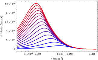
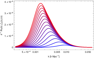
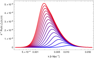
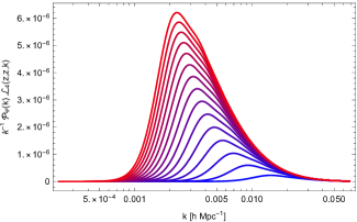
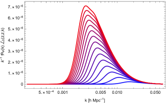
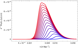
Beside the technical aspects, it is easy to study the behavior of subscript\mathcal{L}_{\ell}’s themselves, such that they can be interpreted as power spectra for each multipole. In Fig. 2 we plot these power spectra for the first six multipoles for the lensing-lensing correlation at the same redshift, which ranges from z=0.15𝑧0.15z=0.15 (bluer) to z=1.55𝑧1.55z=1.55 (redder).

Refer to caption
Refer to caption
Refer to caption
Refer to caption
Refer to caption
Refer to caption
Figure 2: Power spectrum for the different multipoles of the 2-point correlation function of the lensing term. The lowest multipoles are considered: =11\ell=1 (top-left), =22\ell=2 (top-right), =33\ell=3 (center-left), =44\ell=4 (center-right), =55\ell=5 (bottom-left) and =66\ell=6 (bottom-right). The monopole is not shown as it is null for the correlation function of the lensing correction. All these lines refers to the same redshift in the correlation function, ranging from z=0.15𝑧0.15z=0.15 (bottom curves) to z=1.55𝑧1.55z=1.55 (top curves), with an interval step of 0.1. As we can notice, higher multipoles exhibit the presence of a second peak which becomes more important at higher redshifts. These plots show scales ranging from kIR=H0=3×10⁴hMpc1subscript𝑘𝐼𝑅subscript𝐻03superscript104superscriptMpc1k_{IR}=H_{0}=3\times 10^{-4}h\,\text{Mpc}^{-1} to kUV=0.1hMpc1subscript𝑘𝑈𝑉0.1superscriptMpc1k_{UV}=0.1h\,\text{Mpc}^{-1}.

Along these plots, we notice several interesting features:

  • First of all, higher redshifts exhibit higher peaks than closer sources. This is somehow expected, since this behavior just reflects the fact that lensing is an integrated effect, such that the farer the source, the bigger the effect.

  • Secondly, for higher multipoles the peak is drifted towards the smaller scales. This is also expected since higher multipoles investigates the correlation on smaller angular scales. To be mentioned is the behavior for the dipole. Here at larger redshift we notice that a considerable amount of power lies on super-Hubble scales. This leads to a degeneracy between super-Hubble fluctuations and the choice of the background value. This is due to the fact that we have not taken into account corrections due to the observer’s peculiar motion. Indeed, the latter contributes to the dipole and this renders the total 2-point correlation function independent of the physics beyond super-Hubbles scales, restoring causality as shown in Scaccabarozzi et al. (2018). However, as it emerges from Figs. 2, the lensing dipole is comparable to other multipoles only for very low redshifts. Hence, truncation of the angular spectra at =22\ell=2 introduces a negligible error to the lensing contribution to the 2-point correlation function for high redshifts (see also Fig. 4). This method is in line with what suggested in Tansella et al. (2018) and has the practical advantage of getting rid of the dependence on super-Hubble physics and lower the number of terms involved in the analysis.

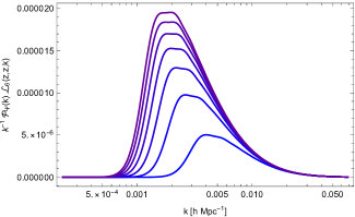
  • Moreover, we notice the appearance of a secondary peak at higher multipoles. The relative importance of the second peak becomes higher for farer sources. This is shown in Fig. 3, where the same plot as in Fig. 2 is done for =66\ell=6 and where the redshift ranges from z=1𝑧1z=1 (bottom) to z=7𝑧7z=7 (top). It is evident how at higher redshift the peaks are such competitive and close that it sounds fairer to refer to a range of scales as the dominant ones rather than just a single peak. According to our understanding, this behavior reflects the fact that on larger multipoles and at higher redshifts, at the given angular scale, there is room for ”resonances” in the k𝑘k-space on the transverse plane wrt to the line-of sight.
Refer to caption
Figure 3: The same as in Fig. 2 for =66\ell=6. Now the redshift ranges from z=1𝑧1z=1 (bottom curve) to z=7𝑧7z=7 (top curve) with a redshift gap of 1. As we can notice, at higher redshift the appearance of a second peak eventually flattens the curves at their maximum.

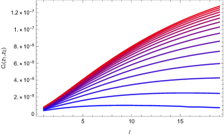
Figs. 2 also indicate that the \ell-expansion converges quite slowly to the full angular correlation function. Indeed, until =66\ell=6 the order of magnitude of the spectra tends to increase or stays constant for the same redshift. This behavior is more evident in the top panel of Fig. 4. Here we plot the first 19 multipoles for the lensing and consider the cross correlation between the sources at redshift z1=0.75subscript𝑧10.75z_{1}=0.75 and other sources with possibly different redshift, letting z2subscript𝑧2z_{2} range from 0.150.150.15 (bluer, bottom) to 1.551.551.55 (redder, top). As we can appreciate from the figure, the order of magnitude for the multipoles at the same redshift tends to remain the same or increase. For what concerns the pair (z1,z2)=(0.15,0.75)subscript𝑧1subscript𝑧20.150.75(z_{1},z_{2})=(0.15,0.75) (bottom curve in Fig. 4), the multipoles decrease in amplitude after 7similar-to7\ell\sim 7. However, this decreasing is not rapid enough to allow convergence to the full result for the chosen first 19 multipoles.
Refer to caption
Refer to caption
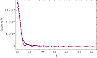
Figure 4: Top-panel: 19 lowest multipoles of the 2-point angular correlation function of lensing. Here the first redshift is fixed at z1=0.75subscript𝑧10.75z_{1}=0.75 whereas the second one z2subscript𝑧2z_{2} varies from 0.150.150.15 (bottom curve) to 1.551.551.55 (top curve), with a redshift step of 0.10.10.1. Bottom-panel: comparison between the numerical evaluation of the 2-point angular correlation function for the lensing (blue points) with the semi-analytical estimation given by the sum of the multipoles truncated at =1919\ell=19 (red curve). Here z1=0.75subscript𝑧10.75z_{1}=0.75 and z2=0.15subscript𝑧20.15z_{2}=0.15. The bottom panel corresponds to the re-summation of multipoles of the bottom curve in the top panel. The comparison between the two figures makes clear that the multipoles for the considered redshift slowly decreases and the cutoff to be chosen in order to truncate the multipole expansion is not yet reached at =1919\ell=19. This behavior is due to the steepness of the peak at ν=1𝜈1\nu=1. The convergence becomes even slower at higher redshift, as shown in the other curves in the top panel.

To make this point clearer, in the bottom panel of Fig. 4 we compare the full numerical estimation of the the angular correlation function at z1=0.15subscript𝑧10.15z_{1}=0.15 and z2=0.75subscript𝑧20.75z_{2}=0.75 (blue points) with its truncated \ell-expansion until =1919\ell=19 (with coefficient given in the bottom curve of the top panel). We realize from this plot that intermediate angular ranges are in an acceptable agreement (modulo an oscillation due to the truncation in the Legendre expansion), whereas the maximum still admits a 15%similar-toabsentpercent15\sim 15\% missing correction. Considering that the numerical value of the peak is 3×1073superscript1073\times 10^{-7} and the order of magnitude of the Csubscript𝐶C_{\ell} for this bin pair is 108superscript10810^{-8}, we can estimate the convergence \ell scale thanks to the argument which follows. The value of the angular correlation at its peak corresponds to the full resummed series of all the Csubscript𝐶C_{\ell}’s for a given redshift pair. This can be understood by looking at the Eq. (30) since Legendre’s polynomials all equal 1 when evaluated at ν=1𝜈1\nu=1. Thanks to a simple analytical estimation, we can then infer that a 1%percent11\% error on the peak’s resolution for the chosen case will be reached around at 50similar-to50\ell\sim 50. The situation is even worse for the other redshift pairs.

Finally, the high value of these convergent angular scales means that the angular correlation function for the lensing is extremely peaked around its maximum and then tends to correlate between light-signals emitted from sources separated by a very narrow angular size.

III.2 Doppler

The same analysis can be done for the Doppler angular correlation function. The analogous of Lsubscriptsuperscript𝐿\mathcal{L}^{L}_{\ell} for the Doppler effect can be written exactly for each multipoles without requiring the polynomial interpolation for g𝑔g. This is due to the fact that Doppler effect is not integrated along the line-of-sight and then the integrations of the growth functions factorizes in the ultimate expression in the functions Gisubscript𝐺𝑖G_{i} in 𝒲PVsubscript𝒲𝑃𝑉\mathcal{W}_{PV} in Eq. (27). This leads to an important difference when compared with lensing. Indeed, for the case of Doppler, PVsubscriptsuperscript𝑃𝑉\mathcal{L}^{PV}_{\ell} can be written as a product of combination of spherical Bessel functions for each \ell, and this product is symmetric under the exchange of zizjsubscript𝑧𝑖subscript𝑧𝑗z_{i}\leftrightarrow z_{j}. Moreover, the dependences on the two redshifts are decoupled. For a matter of clarity, we report the simplest cases of the monopole (=00\ell=0) and dipole (=11\ell=1) for the Doppler

0PV(zi,zj)=subscriptsuperscript𝑃𝑉0subscript𝑧𝑖subscript𝑧𝑗absent\displaystyle\mathcal{L}^{PV}_{0}(z_{i},z_{j})= j1(kΔηi)j1(kΔηj)subscript𝑗1𝑘Δsubscript𝜂𝑖subscript𝑗1𝑘Δsubscript𝜂𝑗\displaystyle\,j_{1}\left(k\Delta\eta_{i}\right)j_{1}\left(k\Delta\eta_{j}\right)
1PV(zi,zj)=subscriptsuperscript𝑃𝑉1subscript𝑧𝑖subscript𝑧𝑗absent\displaystyle\mathcal{L}^{PV}_{1}(z_{i},z_{j})=  3[j1(kΔηi)kΔηij2(kΔηi)]3delimited-[]subscript𝑗1𝑘Δsubscript𝜂𝑖𝑘Δsubscript𝜂𝑖subscript𝑗2𝑘Δsubscript𝜂𝑖\displaystyle\,3\left[\frac{j_{1}\left(k\Delta\eta_{i}\right)}{k\Delta\eta_{i}}-j_{2}\left(k\Delta\eta_{i}\right)\right]
×[j1(kΔηj)kΔηjj2(kΔηj)].absentdelimited-[]subscript𝑗1𝑘Δsubscript𝜂𝑗𝑘Δsubscript𝜂𝑗subscript𝑗2𝑘Δsubscript𝜂𝑗\displaystyle\times\left[\frac{j_{1}\left(k\Delta\eta_{j}\right)}{k\Delta\eta_{j}}-j_{2}\left(k\Delta\eta_{j}\right)\right]\,. (41)

It is worth to remark that Eq. (41) can be written as PV=(2+1)j(kΔηi)j(kΔηj)subscriptsuperscript𝑃𝑉21subscriptsuperscript𝑗𝑘Δsubscript𝜂𝑖subscriptsuperscript𝑗𝑘Δsubscript𝜂𝑗\mathcal{L}^{PV}_{\ell}=\left(2\ell+1\right)j^{\prime}_{\ell}(k\Delta\eta_{i})j^{\prime}_{\ell}(k\Delta\eta_{j}). This is in agreement with results of Bonvin et al. (2006). The same structure occurs for higher multipoles, but with a more involved combination of higher order jnsubscript𝑗𝑛j_{n}. Since the product of jnsubscript𝑗𝑛j_{n}’s shows a constructive interference only when z1z2subscript𝑧1subscript𝑧2z_{1}\approx z_{2}, PVsubscriptsuperscript𝑃𝑉\mathcal{L}^{PV}_{\ell} is mostly positive only when the two redshift are almost the same. For larger separation, PVsubscriptsuperscript𝑃𝑉\mathcal{L}^{PV}_{\ell} exhibits an oscillating behavior which suppresses the integration in k𝑘k-space and reduces the amplitude of multipoles. This explain why Doppler angular correlation is relevant only for sources placed within the same redshift bin. Finally, we comment on the fact that this is not the case for lensing, when the Lsubscriptsuperscript𝐿\mathcal{L}^{L}_{\ell}’s are positive defined also for large angular separation. This is due to the fact that lensing is an integrated effect along the line-of-sight and then also two sources with a separation in redshift space contribute to the amplitude in a non-negligible way.

III.3 Monopoles for the general 2-point correlation function

The above-mentioned features for the spectral decomposition of the 2-point correlation functions can be generalized by evaluating the angular integral over ΩksubscriptΩ𝑘\Omega_{k} in Eq. (22). In fact, since the operators O^Esubscript^𝑂𝐸\hat{O}_{E} do not act on the angular dependences in dΩk𝑑subscriptΩ𝑘d\Omega_{k} in the kernels 𝒲Ei,Ejsubscript𝒲𝐸𝑖superscript𝐸𝑗\mathcal{W}_{Ei,E^{\prime}j}, we can perform this integration independently by aligning the z𝑧z axis of 𝐤𝐤{\bf k} with the vector rEi𝐧irEj𝐧jsubscript𝑟𝐸𝑖subscript𝐧𝑖subscript𝑟superscript𝐸𝑗subscript𝐧𝑗r_{Ei}{\bf n}_{i}-r_{E^{\prime}j}{\bf n}_{j}. We then get

𝑑Ωkei𝐤(rEi𝐧irEj𝐧j)=differential-dsubscriptΩ𝑘superscript𝑒𝑖𝐤subscript𝑟𝐸𝑖subscript𝐧𝑖subscript𝑟superscript𝐸𝑗subscript𝐧𝑗absent\displaystyle\int{d\Omega_{k}}e^{i{\bf k}\cdot(r_{Ei}{\bf n}_{i}-r_{E^{\prime}j}{\bf n}_{j})}= 2π11d(cosθk)eikRcosθk2𝜋superscriptsubscript11𝑑subscript𝜃𝑘superscript𝑒𝑖𝑘𝑅subscript𝜃𝑘\displaystyle 2\pi\int_{-1}^{1}d\left(\cos\theta_{k}\right)e^{ikR\cos\theta_{k}}
=\displaystyle= 4πj0(kR),4𝜋subscript𝑗0𝑘𝑅\displaystyle 4\pi j_{0}(kR)\,, (42)

where R=R(ηE,ηE,ν)𝑅𝑅subscript𝜂𝐸subscript𝜂superscript𝐸𝜈R=R(\eta_{E},\eta_{E^{\prime}},\nu). In this way, Eq. (22) gets the simple expression

𝒲Ei,Ej=O^EiO^Ej[g(ηEi)g(ηo)g(ηEj)g(ηo)j0(kR)].subscript𝒲𝐸𝑖superscript𝐸𝑗subscript^𝑂𝐸𝑖subscript^𝑂superscript𝐸𝑗delimited-[]𝑔subscript𝜂𝐸𝑖𝑔subscript𝜂𝑜𝑔subscript𝜂superscript𝐸𝑗𝑔subscript𝜂𝑜subscript𝑗0𝑘𝑅\mathcal{W}_{Ei,E^{\prime}j}=\hat{O}_{Ei}\hat{O}_{E^{\prime}j}\left[\frac{g(\eta_{Ei})}{g(\eta_{o})}\frac{g(\eta_{E^{\prime}j})}{g(\eta_{o})}j_{0}(kR)\right]\,. (43)

This exact expression is as simple as powerful. Indeed, thanks to Eq. (43), we can generate the kernel for any relativistic effect E𝐸E simply as the action of the operator O^Esubscript^𝑂𝐸\hat{O}_{E} on the function g(ηE)j0(kR)𝑔subscript𝜂𝐸subscript𝑗0𝑘𝑅g(\eta_{E})\,j_{0}(kR). Eq. (43) is also useful since it provides a generating function for the monopole of the ξEEsubscript𝜉𝐸superscript𝐸\xi_{EE^{\prime}}. Indeed, the kernel for the monopole is given by the action of the angular average on the Eq. (43)

𝒲Ei,Ej0=superscriptsubscript𝒲𝐸𝑖superscript𝐸𝑗0absent\displaystyle\mathcal{W}_{Ei,E^{\prime}j}^{0}= 1211𝑑ν𝒲Ei,Ej12superscriptsubscript11differential-d𝜈subscript𝒲𝐸𝑖superscript𝐸𝑗\displaystyle\frac{1}{2}\int_{-1}^{1}d\nu\,\mathcal{W}_{Ei,E^{\prime}j}
=\displaystyle= 1211𝑑νO^EiO^Ej[g(ηEi)g(ηo)g(ηEj)g(ηo)j0(kR)]12superscriptsubscript11differential-d𝜈subscript^𝑂𝐸𝑖subscript^𝑂superscript𝐸𝑗delimited-[]𝑔subscript𝜂𝐸𝑖𝑔subscript𝜂𝑜𝑔subscript𝜂superscript𝐸𝑗𝑔subscript𝜂𝑜subscript𝑗0𝑘𝑅\displaystyle\frac{1}{2}\int_{-1}^{1}d\nu\,\hat{O}_{Ei}\hat{O}_{E^{\prime}j}\left[\frac{g(\eta_{Ei})}{g(\eta_{o})}\frac{g(\eta_{E^{\prime}j})}{g(\eta_{o})}j_{0}(kR)\right]
=\displaystyle= 12O^EiO^Ej[g(ηEi)g(ηo)g(ηEj)g(ηo)11𝑑νj0(kR)]12subscript^𝑂𝐸𝑖subscript^𝑂superscript𝐸𝑗delimited-[]𝑔subscript𝜂𝐸𝑖𝑔subscript𝜂𝑜𝑔subscript𝜂superscript𝐸𝑗𝑔subscript𝜂𝑜superscriptsubscript11differential-d𝜈subscript𝑗0𝑘𝑅\displaystyle\frac{1}{2}\hat{O}_{Ei}\hat{O}_{E^{\prime}j}\left[\frac{g(\eta_{Ei})}{g(\eta_{o})}\frac{g(\eta_{E^{\prime}j})}{g(\eta_{o})}\int_{-1}^{1}d\nu\,j_{0}(kR)\right]
=\displaystyle= O^Ei[g(ηEi)g(ηo)j0(kΔηEi)]subscript^𝑂𝐸𝑖delimited-[]𝑔subscript𝜂𝐸𝑖𝑔subscript𝜂𝑜subscript𝑗0𝑘Δsubscript𝜂𝐸𝑖\displaystyle\hat{O}_{Ei}\left[\frac{g(\eta_{Ei})}{g(\eta_{o})}j_{0}\left(k\Delta\eta_{Ei}\right)\right]
×O^Ej[g(ηEj)g(ηo)j0(kΔηEj)],absentsubscript^𝑂superscript𝐸𝑗delimited-[]𝑔subscript𝜂superscript𝐸𝑗𝑔subscript𝜂𝑜subscript𝑗0𝑘Δsubscript𝜂superscript𝐸𝑗\displaystyle\times\hat{O}_{E^{\prime}j}\left[\frac{g(\eta_{E^{\prime}j})}{g(\eta_{o})}j_{0}\left(k\Delta\eta_{E^{\prime}j}\right)\right]\,, (44)

where we used 11𝑑νj0(kR(x,y,ν))=2j0(kx)j0(ky)superscriptsubscript11differential-d𝜈subscript𝑗0𝑘𝑅𝑥𝑦𝜈2subscript𝑗0𝑘𝑥subscript𝑗0𝑘𝑦\int_{-1}^{1}d\nu j_{0}(kR(x,y,\nu))=2j_{0}(kx)j_{0}(ky). The second-last equality in Eq. (44) is due to the fact that all the O^Esubscript^𝑂𝐸\hat{O}_{E}’s commute with the angular average. Indeed, for what concerns the lensing O^L=Δ2subscript^𝑂𝐿subscriptΔ2\hat{O}_{L}=\Delta_{2}, on one hand we recall that the angular average of the angular Laplacian is null. On the other hand, the angular average of a given function does not depend on the angle, then its Laplacian is null. Provided that, we can commute O^Lsubscript^𝑂𝐿\hat{O}_{L} with the angular average. In regard of all other operators, they do not depend on the angular coordinates, so they can be exchanged as well with the angular average.

The crucial aspect of Eq. (44) is the complete factorization of the effects. This also allows to analytically evaluate the kernels for the monopole contribution due to all the 15 auto and cross 2-point correlation functions thanks to the action of only 5 different operators. In particular, we get

O^PV[g(ηs)g(ηo)j0(kΔηs)]=subscript^𝑂𝑃𝑉delimited-[]𝑔subscript𝜂𝑠𝑔subscript𝜂𝑜subscript𝑗0𝑘Δsubscript𝜂𝑠absent\displaystyle\hat{O}_{PV}\left[\frac{g(\eta_{s})}{g(\eta_{o})}\,j_{0}(k\Delta\eta_{s})\right]= kΞsGsj1(kΔηs)𝑘subscriptΞ𝑠subscript𝐺𝑠subscript𝑗1𝑘Δsubscript𝜂𝑠\displaystyle k\,\Xi_{s}G_{s}\,j_{1}(k\Delta\eta_{s})
O^SW[g(ηs)g(ηo)j0(kΔηs)]=subscript^𝑂𝑆𝑊delimited-[]𝑔subscript𝜂𝑠𝑔subscript𝜂𝑜subscript𝑗0𝑘Δsubscript𝜂𝑠absent\displaystyle\hat{O}_{SW}\left[\frac{g(\eta_{s})}{g(\eta_{o})}\,j_{0}(k\Delta\eta_{s})\right]= (1+Ξs)g(ηs)g(ηo)j0(kΔηs)1subscriptΞ𝑠𝑔subscript𝜂𝑠𝑔subscript𝜂𝑜subscript𝑗0𝑘Δsubscript𝜂𝑠\displaystyle-(1+\Xi_{s})\frac{g(\eta_{s})}{g(\eta_{o})}\,j_{0}(k\Delta\eta_{s})
O^ISW[g(η)g(ηo)j0(kΔη)]=subscript^𝑂𝐼𝑆𝑊delimited-[]𝑔𝜂𝑔subscript𝜂𝑜subscript𝑗0𝑘Δ𝜂absent\displaystyle\hat{O}_{ISW}\left[\frac{g(\eta)}{g(\eta_{o})}\,j_{0}(k\Delta\eta)\right]= 2Ξsηsηo𝑑η(g(η)g(ηo)j0(kΔη)+g(η)g(ηo)j1(kΔη))2subscriptΞ𝑠superscriptsubscriptsubscript𝜂𝑠subscript𝜂𝑜differential-d𝜂superscript𝑔𝜂𝑔subscript𝜂𝑜subscript𝑗0𝑘Δ𝜂𝑔𝜂𝑔subscript𝜂𝑜subscript𝑗1𝑘Δ𝜂\displaystyle-2\,\Xi_{s}\int_{\eta_{s}}^{\eta_{o}}d\eta\left(\frac{g^{\prime}(\eta)}{g(\eta_{o})}\,j_{0}(k\Delta\eta)+\frac{g(\eta)}{g(\eta_{o})}\,j_{1}(k\Delta\eta)\right)
O^TD[g(η)g(ηo)j0(kΔη)]=subscript^𝑂𝑇𝐷delimited-[]𝑔𝜂𝑔subscript𝜂𝑜subscript𝑗0𝑘Δ𝜂absent\displaystyle\hat{O}_{TD}\left[\frac{g(\eta)}{g(\eta_{o})}\,j_{0}(k\Delta\eta)\right]= 2Δηsηsηo𝑑ηg(η)g(ηo)j0(kΔη)2Δsubscript𝜂𝑠superscriptsubscriptsubscript𝜂𝑠subscript𝜂𝑜differential-d𝜂𝑔𝜂𝑔subscript𝜂𝑜subscript𝑗0𝑘Δ𝜂\displaystyle\frac{2}{\Delta\eta_{s}}\int_{\eta_{s}}^{\eta_{o}}d\eta\frac{g(\eta)}{g(\eta_{o})}\,j_{0}(k\Delta\eta)
O^L[g(η)g(ηo)j0(kΔη)]=subscript^𝑂𝐿delimited-[]𝑔𝜂𝑔subscript𝜂𝑜subscript𝑗0𝑘Δ𝜂absent\displaystyle\hat{O}_{L}\left[\frac{g(\eta)}{g(\eta_{o})}\,j_{0}(k\Delta\eta)\right]= 0.0\displaystyle 0\,. (45)

These relations are enough to evaluate the monopole for the whole ξ𝜉\xi. We remark that lensing has no monopole. Hence, from Eqs. (45) and the factorization in Eq. (44) we infer that also all the cross-correlations between lensing and any other relativistic effect in the luminosity distance have vanishing monopole. This has consequences for what concerns the observation of large number of sources distributed all over the sky. Indeed, in the limit of large number of sources, the spatial average tends to the angular ones and then σH02subscriptsuperscript𝜎2subscript𝐻0\sigma^{2}_{H_{0}} is completely given by the sum of the monopoles for each combination of EE𝐸superscript𝐸EE^{\prime}. In this limit, then, any cross-correlation with lensing cannot contribute to the total effect. This independence on lensing is an interesting point, since this is usually one of the most important effect in the analysis of Large Scale Structure surveys.

Total monopole is then expected to be dominated by the auto correlation of Doppler. This indeed is due to the fact that Eqs. (45) exhibits a further k𝑘k in the first line. The latter then contributes with a k2superscript𝑘2k^{2} amplitude in the integration over k𝑘k-space which then contributes more than the other pairs.

We underline that this features of monopoles follows from the fact that P0subscript𝑃0P_{0} is constant. The same analysis can be applied to higher multipoles. However, since Psubscript𝑃P_{\ell}’s in general depend on ν𝜈\nu, they do not commute with all the operators O^Esubscript^𝑂𝐸\hat{O}_{E} (in particular when E=L𝐸𝐿E=L) and this aspect must be taken into account for higher multipoles. The cosmological information within LSS contained in higher multipoles has been discussed in recent papers as Di Dio and Seljak (2019); Beutler and Di Dio (2020), where the dipolar structure of galaxy number counts has been investigated. We postpone the investigation of these effects multipole by multipole within forthcoming surveys to future works. We stress, however, that the analysis performed in the next sections captures the presence of all the multipoles for the 2-point correlation function.

We then conclude this section by remarking that typical surveys have no access to the full sky coverage. This practical limitation makes lensing contribution no longer vanishing and then dominating the other effects. In the following sections, we will show this point and forecast for some cases of interest for forthcoming surveys the expected values for σH02subscriptsuperscript𝜎2subscript𝐻0\sigma^{2}_{H_{0}}.

IV Numerical evaluations

In this section, we will provide numerical evaluation of the 2-point correlation function ξ𝜉\xi. To this aim, we will focus our analysis only on lensing and doppler terms. Indeed, from Eqs. (27) we have that the kernels regarding lensing and doppler effects, namely 𝒲Lsubscript𝒲𝐿\mathcal{W}_{L} and 𝒲PVsubscript𝒲𝑃𝑉\mathcal{W}_{PV}, have the higher number of powers in terms of k𝑘k, respectively k4superscript𝑘4k^{4} and k2superscript𝑘2k^{2}. Moreover, 𝒲PVsubscript𝒲𝑃𝑉\mathcal{W}_{PV} contains the pre-factors ΞΞ\Xi and these amplify the effect on small redshift. Motivated by the same argument, in Eqs. (28) the only term of interest for us is 𝒲PVLsubscript𝒲𝑃𝑉𝐿\mathcal{W}_{PV\,L} which indeed contains the highest number of power in k𝑘k and is amplified by the prefactor ΞΞ\Xi. To this aim, we consider the linear dimensionless power spectrum today

𝒫ψ=A(kk0)ns1925[g(ηo)g]2T2(k13.41keq),subscript𝒫𝜓𝐴superscript𝑘subscript𝑘0subscript𝑛𝑠1925superscriptdelimited-[]𝑔subscript𝜂𝑜subscript𝑔2superscript𝑇2𝑘13.41subscript𝑘eq\mathcal{P}_{\psi}=A\left(\frac{k}{k_{0}}\right)^{n_{s}-1}{9\over 25}\left[\frac{g(\eta_{o})}{g_{\infty}}\right]^{2}T^{2}\left(\frac{k}{13.41\,k_{\text{eq}}}\right)\,, (46)

where T(k)𝑇𝑘T(k) is the so-called transfer function which takes into account the sub-horizon evolution of modes re-entering the horizon during the radiation era. We have expressed T(k)𝑇𝑘T(k) in the Hu-Eisenstein parametrization Eisenstein and Hu (1998), given by

T(q)=𝑇𝑞absent\displaystyle T(q)= L0(q)L0(q)+q2C0(q),subscript𝐿0𝑞subscript𝐿0𝑞superscript𝑞2subscript𝐶0𝑞\displaystyle\frac{L_{0}(q)}{L_{0}(q)+q^{2}\,C_{0}(q)}\,,
L0(q)=subscript𝐿0𝑞absent\displaystyle L_{0}(q)= log(2e+1.8q),2𝑒1.8𝑞\displaystyle\log(2\,e+1.8\,q)\,,
C0(q)=subscript𝐶0𝑞absent\displaystyle C_{0}(q)= 14.2+7311+62.5q.14.2731162.5𝑞\displaystyle 14.2+\frac{731}{1+62.5\,q}\,. (47)

We have integrated over the spectral distribution of frequency modes using the following infrared (IR) and ultraviolet (UV) cutoff values:

kIR=3×10⁴hMpc1,kUV=0.1×hMpc1.formulae-sequencesubscript𝑘IR3superscript104superscriptMpc1subscript𝑘UV0.1superscriptMpc1k_{\rm IR}=3\times 10^{-4}\,h\,{\rm Mpc}^{-1},~{}~{}~{}~{}~{}~{}~{}~{}k_{\rm UV}=0.1\times h\,{\rm Mpc}^{-1}. (48)

They roughly correspond to the present horizon scale and to the limiting scale of the linear spectral regime, respectively. The numerical values of the parameters appearing in Eqs. (17), (46) and (47) have been chosen, according to recent cosmological observations Aghanim et al. (2020), as follows

A=𝐴absent\displaystyle A=  2.2×10⁹,ns=0.96,k0=0.05Mpc1,formulae-sequence2.2superscript109subscript𝑛𝑠0.96subscript𝑘00.05superscriptMpc1\displaystyle\,2.2\times 10^{-9},\quad n_{s}=0.96,\quad k_{0}=0.05\,\text{Mpc}^{-1},
keq=subscript𝑘eqabsent\displaystyle k_{\text{eq}}= 0.07h2Ωm0,h= 0.68,Ωm0=0.315.formulae-sequence0.07superscript2subscriptΩ𝑚00.68subscriptΩ𝑚00.315\displaystyle 0.07\,h^{2}\,\Omega_{m0},\quad h=\,0.68,\quad\Omega_{m0}=0.315\,. (49)

With these numerical specifications, we first want to plot the values for aligned (ν=1𝜈1\nu=1) and antipodes (ν=1𝜈1\nu=-1) correlation regarding ξLsuperscript𝜉𝐿\xi^{L}, ξPVsuperscript𝜉𝑃𝑉\xi^{PV} and ξPV,Lsuperscript𝜉𝑃𝑉𝐿\xi^{PV,L}. To this aim, we underline that these explicit limits ν=±1𝜈plus-or-minus1\nu=\pm 1 show a huge analytic simplification for 𝒲Lsubscript𝒲𝐿\mathcal{W}_{L}, 𝒲PVsubscript𝒲𝑃𝑉\mathcal{W}_{PV} and 𝒲PV,Lsubscript𝒲𝑃𝑉𝐿\mathcal{W}_{PV,\,L} in Eqs. (27), (28) and (34). We find indeed that those kernels become

𝒲PVij±subscriptsuperscript𝒲plus-or-minus𝑃𝑉𝑖𝑗\displaystyle\mathcal{W}^{\pm}_{PVij} =±13ΞiΞjGiGjk2[j02j2](k(ΔηiΔηj))absentplus-or-minus13subscriptΞ𝑖subscriptΞ𝑗subscript𝐺𝑖subscript𝐺𝑗superscript𝑘2delimited-[]subscript𝑗02subscript𝑗2𝑘minus-or-plusΔsubscript𝜂𝑖Δsubscript𝜂𝑗\displaystyle=\pm\,\frac{1}{3}\Xi_{i}\Xi_{j}G_{i}G_{j}k^{2}\left[j_{0}-2j_{2}\right]\left(k(\Delta\eta_{i}\mp\Delta\eta_{j})\right)
𝒲Lij±=subscriptsuperscript𝒲plus-or-minus𝐿𝑖𝑗absent\displaystyle\mathcal{W}^{\pm}_{Lij}= 1Δηi1Δηj0Δηi𝑑xΔηixx0Δηj𝑑yΔηjyyg(ηox)g(ηoy)g2(ηo)[k28x2y2(xy)2j2±4kxyxyj1](k(xy))1Δsubscript𝜂𝑖1Δsubscript𝜂𝑗superscriptsubscript0Δsubscript𝜂𝑖differential-d𝑥Δsubscript𝜂𝑖𝑥𝑥superscriptsubscript0Δsubscript𝜂𝑗differential-d𝑦Δsubscript𝜂𝑗𝑦𝑦𝑔subscript𝜂𝑜𝑥𝑔subscript𝜂𝑜𝑦superscript𝑔2subscript𝜂𝑜delimited-[]plus-or-minussuperscript𝑘28superscript𝑥2superscript𝑦2superscriptminus-or-plus𝑥𝑦2subscript𝑗24𝑘𝑥𝑦minus-or-plus𝑥𝑦subscript𝑗1𝑘minus-or-plus𝑥𝑦\displaystyle\frac{1}{\Delta\eta_{i}}\frac{1}{\Delta\eta_{j}}\int_{0}^{\Delta\eta_{i}}dx\frac{\Delta\eta_{i}-x}{x}\int_{0}^{\Delta\eta_{j}}dy\frac{\Delta\eta_{j}-y}{y}\frac{g(\eta_{o}-x)g(\eta_{o}-y)}{g^{2}(\eta_{o})}\Big{[}k^{2}8\frac{x^{2}\,y^{2}}{(x\mp y)^{2}}j_{2}\pm 4\,k\,\frac{x\,y}{x\mp y}\,j_{1}\Big{]}\left(k(x\mp y)\right)
WPVi,Lj±=subscriptsuperscript𝑊plus-or-minus𝑃𝑉𝑖𝐿𝑗absent\displaystyle{W}^{\pm}_{PVi,Lj}= ΞiΔηjGi0ΔηjdxΔηjxxg(ηox)g(ηo){k3x2j3\displaystyle\frac{\Xi_{i}}{\Delta\eta_{j}}G_{i}\int_{0}^{\Delta\eta_{j}}dx\frac{\Delta\eta_{j}-x}{x}\frac{g(\eta_{o}-x)}{g(\eta_{o})}\Bigg{\{}-k^{3}x^{2}j_{3}
+k2x(3xΔηix2)j2kxΔηix[k2x(Δηix)2]j1}(k(Δηix)),\displaystyle+k^{2}x\left(3\frac{x}{\Delta\eta_{i}\mp x}\mp 2\right)j_{2}-\frac{k\,x}{\Delta\eta_{i}\mp x}\left[k^{2}x(\Delta\eta_{i}\mp x)\mp 2\right]j_{1}\Bigg{\}}\left(k(\Delta\eta_{i}\mp x)\right)\,, (50)

where ±plus-or-minus\pm stands for ν=±1𝜈plus-or-minus1\nu=\pm 1 and, in the last lines of Eqs. (50), we have performed the change x=ηoη𝑥subscript𝜂𝑜𝜂x=\eta_{o}-\eta in the integration variable. A further simplification can be done for both 𝒲L±subscriptsuperscript𝒲plus-or-minus𝐿\mathcal{W}^{\pm}_{L} and 𝒲PV,L±subscriptsuperscript𝒲plus-or-minus𝑃𝑉𝐿\mathcal{W}^{\pm}_{PV,L} about the growth function g𝑔g. Just as done for the multipoles in the previous section, we can analytically perform the integrals along the line-of-sight thanks to the polynomial expansion of g(ηox)𝑔subscript𝜂𝑜𝑥g(\eta_{o}-x). This decreases the computational time, since it reduces the evaluation of the function to only 1-dimensional numerical integration in k𝑘k-space. Results are shown in Fig. 5.

Numerical evaluation in the range of redshift of interest for forthcoming surveys (0.15z3.850.15𝑧3.850.15\leq z\leq 3.85) show that lensing and doppler are competitive effects for redshift smaller than 1. Moreover, cross-correlations between these two effects are always negligible in the explored ranges of z𝑧z. According to this, one might conclude that the contributions due to doppler correction are important. However, doppler terms are counterbalanced by the change in sign which occurs around z=1.6𝑧1.6z=1.6 and this leads to a suppression of the total contribution of doppler in deeper surveys. This cancellation can be analytically understood by looking at the explicit expressions involving PV in Eqs. (27) and (28). Indeed, whenever doppler appears in the 2-point correlation function, it shows a factor Ξ=11ΔηΞ11Δ𝜂\Xi=1-\frac{1}{\mathcal{H}\Delta\eta} in the expression of ξEEsuperscript𝜉𝐸superscript𝐸\xi^{EE^{\prime}}. This coefficient is null precisely when Δη=1Δ𝜂superscript1\Delta\eta=\mathcal{H}^{-1} and changes sign. According to our chosen cosmology in Eq. (49), this switch happens exactly at z=1.6𝑧1.6z=1.6 as it is shown in Fig. 5.

Refer to caption
Refer to caption
Refer to caption
Refer to caption
Refer to caption
Refer to caption
Figure 5: Aligned-correlations (ν=1𝜈1\nu=1, right panels) and antipodes-correlations (ν=1𝜈1\nu=-1, left panels) as function of redshift. Thin solid lines refers to positive values as specified by the relative label. In the same way, dashed lines refers to negative values. Thick solid lines refers to the redshifts where correlations are null. We notice that the effect involving doppler terms (middle and bottom ones) always exhibit a null value when the redshift for the doppler effect is z1.6𝑧1.6z\approx 1.6. This value corresponds to the scale where Ξs=0subscriptΞ𝑠0\Xi_{s}=0, namely Δηs=s1Δsubscript𝜂𝑠subscriptsuperscript1𝑠\Delta\eta_{s}=\mathcal{H}^{-1}_{s}. Figures refer to lensing (top panels), doppler (middle panels) and cross-correlation between lensing and doppler (bottom panels). In the regime of interest for us, lensing is always leading with respect to the other terms for the aligned-correlations, whereas doppler turns out to be the leading effect for the antipodes-correlation at redshift smaller than 1. Plots for doppler effect terms are shown in logarithmic scales in order to show better the scaling of their values.

Another important feature that comes from the numerical estimations is that close line-of-sights are more correlated than distant ones for what concerns lensing effect. This behavior is more evident for higher redshift. This then means that ξLijsuperscript𝜉𝐿𝑖𝑗\xi^{Lij} is highly peaked when ν1𝜈1\nu\approx 1 and rapidly decays to the constant value taken at ν=1𝜈1\nu=-1. The angular scales νthijsubscriptsuperscript𝜈𝑖𝑗𝑡\nu^{ij}_{th} at which this decay occurs can be estimated by the following approximation method. We build an approximated ξappLijsubscriptsuperscript𝜉𝐿𝑖𝑗𝑎𝑝𝑝\xi^{Lij}_{app} as

ξappLij(ν)=Θ(νthijν)|ξ+Lij|Θ(ννthij)|ξLij|,subscriptsuperscript𝜉𝐿𝑖𝑗𝑎𝑝𝑝𝜈Θsubscriptsuperscript𝜈𝑖𝑗𝑡𝜈subscriptsuperscript𝜉𝐿𝑖𝑗Θ𝜈subscriptsuperscript𝜈𝑖𝑗𝑡subscriptsuperscript𝜉𝐿𝑖𝑗\xi^{Lij}_{app}(\nu)=\Theta(\nu^{ij}_{th}-\nu)\left|\xi^{Lij}_{+}\right|-\Theta(\nu-\nu^{ij}_{th})\left|\xi^{Lij}_{-}\right|\,, (51)

where Θ(x)Θ𝑥\Theta(x) is the Heaviside step function and subscripts in ξ+subscript𝜉\xi_{+} and ξsubscript𝜉\xi_{-} respectively indicate ν=+1𝜈1\nu=+1 and ν=1𝜈1\nu=-1. Eq. (51) shares the same extremes of ξLijsuperscript𝜉𝐿𝑖𝑗\xi^{Lij} shown in Fig. 5. Moreover, νthijsubscriptsuperscript𝜈𝑖𝑗𝑡\nu^{ij}_{th} is determined by the further requirement that the angular average over the full sky of ξappLijsubscriptsuperscript𝜉𝐿𝑖𝑗𝑎𝑝𝑝\xi^{Lij}_{app} is null, just as what is analytically shown for ξLijsuperscript𝜉𝐿𝑖𝑗\xi^{Lij}, namely

11𝑑νξappLij(ν)=0.superscriptsubscript11differential-d𝜈subscriptsuperscript𝜉𝐿𝑖𝑗𝑎𝑝𝑝𝜈0\int_{-1}^{1}d\nu\,\xi^{Lij}_{app}(\nu)=0\,. (52)

Indeed, by combining Eqs. (51) and (52), we have that

(1νthij)|ξ+Lij|=(νthij+1)|ξLij|1subscriptsuperscript𝜈𝑖𝑗𝑡subscriptsuperscript𝜉𝐿𝑖𝑗subscriptsuperscript𝜈𝑖𝑗𝑡1subscriptsuperscript𝜉𝐿𝑖𝑗\left(1-\nu^{ij}_{th}\right)\left|\xi^{Lij}_{+}\right|=\left(\nu^{ij}_{th}+1\right)\left|\xi^{Lij}_{-}\right|\, (53)

which then returns

νthij=|ξ+Lij||ξLij||ξ+Lij|+|ξLij|.subscriptsuperscript𝜈𝑖𝑗𝑡subscriptsuperscript𝜉𝐿𝑖𝑗subscriptsuperscript𝜉𝐿𝑖𝑗subscriptsuperscript𝜉𝐿𝑖𝑗subscriptsuperscript𝜉𝐿𝑖𝑗\nu^{ij}_{th}=\frac{\left|\xi^{Lij}_{+}\right|-\left|\xi^{Lij}_{-}\right|}{\left|\xi^{Lij}_{+}\right|+\left|\xi^{Lij}_{-}\right|}\,. (54)

From top panels of Fig. 5, we notice that |ξ+Lij||ξLij|much-greater-thansubscriptsuperscript𝜉𝐿𝑖𝑗subscriptsuperscript𝜉𝐿𝑖𝑗\left|\xi^{Lij}_{+}\right|\gg\left|\xi^{Lij}_{-}\right| so νthijsubscriptsuperscript𝜈𝑖𝑗𝑡\nu^{ij}_{th} is expected to be very close but lower than 1. In Fig. 6 we show the numerical values for the range of redshift of our interest.
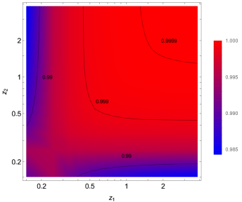
Refer to caption
Figure 6: Plot of νthijsubscriptsuperscript𝜈𝑖𝑗𝑡\nu^{ij}_{th} for the lensing 2-point correlation function. As we can see, ξLijsuperscript𝜉𝐿𝑖𝑗\xi^{Lij} rapidly peaks at values close to ν=1𝜈1\nu=1.

This gives us a threshold angular scale. Redshift by redshift, beyond this angular scale the lensing 2-point correlation function for a given pair of sources is negligible.

The previous estimation is very powerful, since νthijsubscriptsuperscript𝜈𝑖𝑗𝑡\nu^{ij}_{th} can be directly compared with the angular sky coverage of a given survey and tell whether the lensing effect is important or not for the chosen catalog. As an instance, for the EDS configuration, the angular sky coverage is approximatively 20 deg220superscript deg220\text{ deg}^{2} per observation patch Laureijs et al. (2011). This solid angle can be associated to a typical cosine as 20=(180π)202π𝑑ϕνEDS1𝑑ν=2×1802(1νEDS)/π20superscript180𝜋2superscriptsubscript02𝜋differential-ditalic-ϕsuperscriptsubscriptsubscript𝜈𝐸𝐷𝑆1differential-d𝜈2superscript18021subscript𝜈𝐸𝐷𝑆𝜋20=\left(\frac{180}{\pi}\right)^{2}\int_{0}^{2\pi}d\phi\int_{\nu_{EDS}}^{1}d\nu=2\times 180^{2}(1-\nu_{EDS})/\pi, which returns νEDS=0.999subscript𝜈𝐸𝐷𝑆0.999\nu_{EDS}=0.999. From Figs. 6, we notice that νEDSsubscript𝜈𝐸𝐷𝑆\nu_{EDS} is lower than any angular scale at z>0.5𝑧0.5z>0.5. Hence, in this range the narrow sky coverage of EDS is larger than the angular scales where ξLijsuperscript𝜉𝐿𝑖𝑗\xi^{Lij} is at its maximum. On the other hand, when one of the two sources stands at redshift z<0.5𝑧0.5z<0.5, νEDSsubscript𝜈𝐸𝐷𝑆\nu_{EDS} is always greater than νthijsubscriptsuperscript𝜈𝑖𝑗𝑡\nu^{ij}_{th}. In this regard, the approximation of ξLijsuperscript𝜉𝐿𝑖𝑗\xi^{Lij} with ξappLijsubscriptsuperscript𝜉𝐿𝑖𝑗𝑎𝑝𝑝\xi^{Lij}_{app} is expected to work quite well when one of the source is at redshift closer than 0.5. For fainter sources, the fact that we deal with very narrow line-of-sight might show the limit of our approximation. We remark that for larger sky-coverage, just like LSST, our approximation is expected to work well at any redshift. We argue this since larger angular openings tend to full-sky coverages and in this limit case the lensing 2-point correlation function is expected to be null and the peculiar sources located at the transition scales become statistically less significant. We will quantify all these aspects in the next section.

Finally, we conclude this section by underlining the importance of the numerical approximation presented in Eq. (51). The analytical estimation of ξ±Lijsubscriptsuperscript𝜉𝐿𝑖𝑗plus-or-minus\xi^{Lij}_{\pm} with the polynomial expansion of the growth function is numerically very easy to implement. Indeed, it requires only 1-D numerical integration in k𝑘k-space and nothing else. Hence, in spite of its simplicity, the fitting function in Eq. (51) is powerful since its three parameters can be evaluated quickly for different cosmological parameters and then easily implemented in the Montecarlo analysis, where several runs over different cosmologies need to be accessible in short time. With the exact analytical expression of ξLijsuperscript𝜉𝐿𝑖𝑗\xi^{Lij}, the multiple line-of-sight integrals are a huge obstacle in this regard. We finally underline that this fitting method works well only for lensing 2-point correlation function. This is due to the particular features that lensing effect is very peaked for two narrow line-of-sights and its angular average on the full sky is zero. Neither of these properties simultaneously occurs for any other effect here considered. However, this method remains powerful since lensing is anyway the leading effect among all.

In the next section, we will provide some forecast for the σH02subscriptsuperscript𝜎2subscript𝐻0\sigma^{2}_{H_{0}} for the case of the forthcoming surveys EDS and LSST. Finally, we will show the goodness of our fitting function in Eq. (51) in the estimation of σH02subscriptsuperscript𝜎2subscript𝐻0\sigma^{2}_{H_{0}} itself.

V A First Estimation for Next Generation Surveys

In this section, we want to apply the analytical and numerical results previously obtained to the case of Superluminous Supernovae (SLSNe). In particular, we will consider technical aspects for the forthcoming surveys of EDS Laureijs et al. (2011) and LSST Abell et al. (2009). In this regard, we will follow the expected detection rate of SLSNe claimed in Inserra et al. (2021) which we report in Fig. 7.
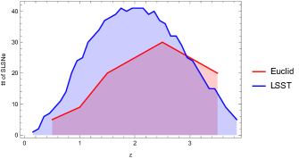
Refer to caption
Figure 7: Simulated SLSNe distributions for Euclid Deep Survey and LSST. From Inserra et al. (2021).

Having these histograms in mind, we generated two random surveys for the distribution of SLSNe with the following specifics

  • 135 sources from EDS are generated in 7 redshift bins where 0.5z3.50.5𝑧3.50.5\leq z\leq 3.5 and the redshift bin width is assumed to be Δz=0.5Δ𝑧0.5\Delta z=0.5. For this survey, the angular distribution covers two line-of-sights at North and South Poles, with angular opening of 20 deg2 per line-of-sight,

  • 929 sources from LSST are generated in 38 redshift bins where 0.15z3.850.15𝑧3.850.15\leq z\leq 3.85 and the redshift bin width is assumed to be Δz=0.1Δ𝑧0.1\Delta z=0.1. For this survey, the angular distribution spans a broad solid angle of 9000 deg2.

Results are summarized in Table 1.

σH02/H02subscriptsuperscript𝜎2subscript𝐻0subscriptsuperscript𝐻20\sigma^{2}_{H_{0}}/H^{2}_{0} EDS LSST
Lensing 5.1×1065.1superscript1065.1\times 10^{-6} 7.6×1087.6superscript1087.6\times 10^{-8}
Doppler 2.1×1092.1superscript1092.1\times 10^{-9} 2.9×10102.9superscript10102.9\times 10^{-10}
Approximated Lensing 3×1063superscript1063\times 10^{-6} 7.1×1087.1superscript1087.1\times 10^{-8}
Table 1: Forecasts for the variance of H0subscript𝐻0H_{0} in EDS and LSST. In the first line, exact 2-point correlation function for lensing is considered. In the second line, there are the contributions from 2-point correlation function of peculiar velocities. In the last line, the expected error from our approximated 2-point correlation function of lensing in Eq. (51) are shown. These values translate in the following values for the dispersion: for EDS, σH0/H0=0.002subscript𝜎subscript𝐻0subscript𝐻00.002\sigma_{H_{0}}/H_{0}=0.002 for the exact estimation and σH0/H0=0.002subscript𝜎subscript𝐻0subscript𝐻00.002\sigma_{H_{0}}/H_{0}=0.002 for the approximated estimation. For LSST, σH0/H0=0.0003subscript𝜎subscript𝐻0subscript𝐻00.0003\sigma_{H_{0}}/H_{0}=0.0003 for the exact estimation and σH0/H0=0.0003subscript𝜎subscript𝐻0subscript𝐻00.0003\sigma_{H_{0}}/H_{0}=0.0003 for the approximated estimation.

Here we see that the dispersion associated to the measure of H0subscript𝐻0H_{0}, namely σH0σH02subscript𝜎subscript𝐻0subscriptsuperscript𝜎2subscript𝐻0\sigma_{H_{0}}\equiv\sqrt{\sigma^{2}_{H_{0}}} is of 0.2%similar-toabsentpercent0.2\sim 0.2\% for EDS but its value drops of almost 1 order of magnitude for LSST, where it contributes with a dispersion of 0.03%similar-toabsentpercent0.03\sim 0.03\%. This significant decrease can be understood by recalling that, for larger sky coverage and large number of sources, the total effect due to lensing must tend to 0. In fact, the specific of LSST are precisely along this direction. Indeed, the number of sources adopted in our forecast of LSST is almost 1 order of magnitude higher than the one of EDS. Furthermore, also the sky coverage is larger.

Another fact that we underline is that doppler effect is always subdominant. Hence we have that the total cosmic variance due to lensing and doppler is

σH0=subscript𝜎subscript𝐻0absent\displaystyle\sigma_{H_{0}}= σH0L2+σH0PV2subscriptsuperscript𝜎2subscript𝐻0𝐿subscriptsuperscript𝜎2subscript𝐻0𝑃𝑉\displaystyle\sqrt{\sigma^{2}_{H_{0}L}+\sigma^{2}_{H_{0}PV}}
\displaystyle\approx σH0L[1+12σH0PV2σH0L2+𝒪((σH0PV2σH0L2)2)].subscript𝜎subscript𝐻0𝐿delimited-[]112subscriptsuperscript𝜎2subscript𝐻0𝑃𝑉subscriptsuperscript𝜎2subscript𝐻0𝐿𝒪superscriptsubscriptsuperscript𝜎2subscript𝐻0𝑃𝑉subscriptsuperscript𝜎2subscript𝐻0𝐿2\displaystyle\sigma_{H_{0}L}\left[1+\frac{1}{2}\frac{\sigma^{2}_{H_{0}PV}}{\sigma^{2}_{H_{0}L}}+\mathcal{O}\left(\left(\frac{\sigma^{2}_{H_{0}PV}}{\sigma^{2}_{H_{0}L}}\right)^{2}\right)\right]\,. (55)

Again from Table 1, we then get that the doppler effect corrects the total cosmic variance associated to H0subscript𝐻0H_{0} by 0.2%percent0.20.2\% for LSST and by 0.02%percent0.020.02\% for EDS.

A further remark is about our approximation scheme for lensing proposed in Eq. (51). From Table 1, we see that the approximated method is in reasonable agreement with the exact evaluation done for LSST. The situation gets worse for EDS. We address this behavior to the specific sky coverage for the chosen surveys. Indeed, for EDS, the sky coverage is quite narrow and comparable for the redshift of our interest with the threshold scales estimated by νthijsubscriptsuperscript𝜈𝑖𝑗𝑡\nu^{ij}_{th}. This implies that the particular details of the angular dependence in ξL(ν)superscript𝜉𝐿𝜈\xi^{L}(\nu) are quite relevant. On the opposite case, LSST has a very broader angular opening. In this case, the sources are distributed with a larger angular opening and this renders the estimation of σH0Lsubscript𝜎subscript𝐻0𝐿\sigma_{H_{0}L} less sensible to the specific values of νthijsubscriptsuperscript𝜈𝑖𝑗𝑡\nu^{ij}_{th}.

Finally, we comment on the limit ideal case of full-sky coverage777See Yoo (2020) for a detailed discussion of this ideal case.. For a large number of sources, lensing never contributes to the 2-point correlation function and then the leading correction is entirely addressed to the monopole of ξPVsuperscript𝜉𝑃𝑉\xi^{PV}. This can be easily evaluated from the kernel in Eq. (41) and results are shown in Fig. 8.
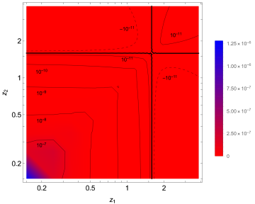
Refer to caption
Figure 8: Monopole of the doppler 2-point correlation function. Thick black lines indicate where function is 0. Dashed lines stand for negative values whereas continues lines refer to positive values.

In this ideal case, σH0subscript𝜎subscript𝐻0\sigma_{H_{0}} is entirely given by the doppler 2-point correlation function. According to the redshift distribution of LSST, we get that σH0/H0=5.6×106subscript𝜎subscript𝐻0subscript𝐻05.6superscript106\sigma_{H_{0}}/H_{0}=5.6\times 10^{-6}.

V.1 Non-linear scales

So far we have taken into account only the linear power spectrum in our analysis. However, non-linear physics can affect significantly the amplitude of lensing (see, for instance Ben-Dayan et al. (2013)). Hence, it is important to understand how much our results are robust when non-linear scales in the power spectrum are taken into account. To this aim, we first adopt the approximation scheme outlined in Eq. (51). In this case, since non-linear scales can enhance lensing up to 1 order of magnitude, we might naively expect that non-linear scales amplify our estimation for σH0subscript𝜎subscript𝐻0\sigma_{H_{0}} by a factor 1010\sqrt{10}. However, this estimation is too much conservative.

A more refined investigation about non-linear scales can be done just by looking at the kernels 𝒲Lij±subscriptsuperscript𝒲plus-or-minus𝐿𝑖𝑗\mathcal{W}^{\pm}_{Lij} in Eqs. (50). Indeed, these are controlled by the functions j1(z)/zsubscript𝑗1𝑧𝑧j_{1}(z)/z and j2(z)/z2subscript𝑗2𝑧superscript𝑧2j_{2}(z)/z^{2}. Both these functions have their maxima in z=0𝑧0z=0 and then oscillate around 0. Hence, they mostly contribute to the integrand when their argument is 𝒪(1)𝒪1\mathcal{O}(1). For the antipodes-correlation, from Eq. (51), we get that the argument of the jnsubscript𝑗𝑛j_{n}’s is k(x+y)𝑘𝑥𝑦k(x+y). Hence, the most relevant part of the integrand occurs when k(x+y)1similar-to𝑘superscript𝑥𝑦1k\sim(x+y)^{-1}. It follows then that small scales contribute to ξLijsubscriptsuperscript𝜉𝐿𝑖𝑗\xi^{Lij}_{-} only at very low redshifts, when x+y𝑥𝑦x+y approaches 0. On top of that, both jnsubscript𝑗𝑛j_{n}’s in 𝒲Lijsubscriptsuperscript𝒲𝐿𝑖𝑗\mathcal{W}^{-}_{Lij} are multiplied by power of xy𝑥𝑦xy. This means that a competitive behavior occurs at low redshifts along the line-of-sight integrations and small scales tend to be suppressed in the ultimate evaluation. Thanks to this argument, we can infer that the value of ξLijsubscriptsuperscript𝜉𝐿𝑖𝑗\xi^{Lij}_{-} is quite insensitive to the small scales and then ξLijsubscriptsuperscript𝜉𝐿𝑖𝑗\xi^{Lij}_{-} does not change dramatically when non-linearities are taken into account.

On the contrary, the jnsubscript𝑗𝑛j_{n}’s in 𝒲Lij+subscriptsuperscript𝒲𝐿𝑖𝑗\mathcal{W}^{+}_{Lij} depend on k(xy)𝑘𝑥𝑦k(x-y). This means that the integrand of ξ+Lijsubscriptsuperscript𝜉𝐿𝑖𝑗\xi^{Lij}_{+} is heavily sourced when xy𝑥𝑦x\approx y. If we call d=xy𝑑𝑥𝑦d=x-y, we get that the jnsubscript𝑗𝑛j_{n}’s gives a non-negligible contribution to the total ξ+Lijsubscriptsuperscript𝜉𝐿𝑖𝑗\xi^{Lij}_{+} whenever kd1similar-to𝑘superscript𝑑1k\sim d^{-1}. This implies that, along the line-of-sight integrations, the smaller the d𝑑d, the higher the contribution from higher k𝑘k. Hence, ξ+Lijsubscriptsuperscript𝜉𝐿𝑖𝑗\xi^{Lij}_{+} is strongly dependent on the smaller scales. This is in line with the fact that non-linearities are expected to heavily source lensing. From our analysis, it turns out that this is true only for ν=1𝜈1\nu=1, namely when two sources are aligned.

The fact that ξ+Lijsubscriptsuperscript𝜉𝐿𝑖𝑗\xi^{Lij}_{+} is highly sensitive to non-linear scales whereas ξLijsubscriptsuperscript𝜉𝐿𝑖𝑗\xi^{Lij}_{-} is almost independent of them has relevant implications on the angular correlation scales νthijsubscriptsuperscript𝜈𝑖𝑗𝑡\nu^{ij}_{th}. Indeed, since the fact that lensing vanishes when integrated all around the observed sky is a pure geometrical effect, hence independent of the investigated scales, Eq. (54) is still a viable approximation. Then we get that the contribution from non-linear scales constrains νthijsubscriptsuperscript𝜈𝑖𝑗𝑡\nu^{ij}_{th} to be closer to one. In fact, when |ξLij||ξ+Lij|much-less-thansubscriptsuperscript𝜉𝐿𝑖𝑗subscriptsuperscript𝜉𝐿𝑖𝑗|\xi^{Lij}_{-}|\ll|\xi^{Lij}_{+}|, Eq. (54) can be expanded as

νthij12|ξLij||ξ+Lij|.subscriptsuperscript𝜈𝑖𝑗𝑡12subscriptsuperscript𝜉𝐿𝑖𝑗subscriptsuperscript𝜉𝐿𝑖𝑗\nu^{ij}_{th}\approx 1-2\frac{|\xi^{Lij}_{-}|}{|\xi^{Lij}_{+}|}\,. (56)

In this way, if the only effect of non-linearities is to increase |ξ+Lij|subscriptsuperscript𝜉𝐿𝑖𝑗|\xi^{Lij}_{+}|, for instance, by a factor C𝐶C, the angular scales conversely tends to 1 with a factor C1superscript𝐶1C^{-1}. We then have two competitive effects: on one hand, the maximum of the 2-point correlation function increases. On the other hand, the angular scales involved in this enhancement are less. Moreover, the product (1νth)|ξ+Lij|2|ξLij|1subscript𝜈𝑡subscriptsuperscript𝜉𝐿𝑖𝑗2subscriptsuperscript𝜉𝐿𝑖𝑗(1-\nu_{th})|\xi^{Lij}_{+}|\approx 2|\xi^{Lij}_{-}| is insensitive to the UV scales. As a consequence, due to non-linear effects in the power spectrum, only sources located almost along the same line-of sight show a non-negligible correction.

To test our arguments, we have then adopted the approximation method outlined in Eqs. (51) and assumed that ξLijsubscriptsuperscript𝜉𝐿𝑖𝑗\xi^{Lij}_{-} remains the same as for the linear spectrum, whereas the net effect of non-linearities is to amplify ξ+Lijsubscriptsuperscript𝜉𝐿𝑖𝑗\xi^{Lij}_{+} by an overall factor 10. With this approach, we find that σH0NL2=7.8×10⁶H02subscriptsuperscript𝜎2subscript𝐻0𝑁𝐿7.8superscript106subscriptsuperscript𝐻20\sigma^{2}_{H_{0}\,NL}=7.8\times 10^{-6}\,H^{2}_{0} for EDS and σH0NL2=6.4×10⁷H02subscriptsuperscript𝜎2subscript𝐻0𝑁𝐿6.4superscript107subscriptsuperscript𝐻20\sigma^{2}_{H_{0}\,NL}=6.4\times 10^{-7}\,H^{2}_{0} for LSST. Hence, within the specific of LSST σH02subscriptsuperscript𝜎2subscript𝐻0\sigma^{2}_{H_{0}} is indeed enhanced by almost one order of magnitude, whereas for EDS σH02subscriptsuperscript𝜎2subscript𝐻0\sigma^{2}_{H_{0}} increases by almost a factor 1.5.

Despite of its rudeness, our analytical estimation agrees very well with the exact estimation where we have chosen kUV=10hsubscript𝑘𝑈𝑉10k_{UV}=10\,h Mpc-1 and set a non-linear power spectrum with the HaloFit model Smith et al. (2003); Takahashi et al. (2012). In this case we obtain σH0NL2=1.1×10⁵H02subscriptsuperscript𝜎2subscript𝐻0𝑁𝐿1.1superscript105subscriptsuperscript𝐻20\sigma^{2}_{H_{0}\,NL}=1.1\times 10^{-5}\,H^{2}_{0} for EDS and σH0NL2=7.8×10⁷H02subscriptsuperscript𝜎2subscript𝐻0𝑁𝐿7.8superscript107subscriptsuperscript𝐻20\sigma^{2}_{H_{0}\,NL}=7.8\times 10^{-7}\,H^{2}_{0} for LSST. Moreover, we have also applied the approximated formula in Eq. (51) with the non-linear values for ξ+Lijsubscriptsuperscript𝜉𝐿𝑖𝑗\xi^{Lij}_{+} and ξLijsubscriptsuperscript𝜉𝐿𝑖𝑗\xi^{Lij}_{-} and we find that σH0NL2=9.4×10⁶H02subscriptsuperscript𝜎2subscript𝐻0𝑁𝐿9.4superscript106subscriptsuperscript𝐻20\sigma^{2}_{H_{0}\,NL}=9.4\times 10^{-6}\,H^{2}_{0} for EDS and σH0NL2=7.8×10⁷H02subscriptsuperscript𝜎2subscript𝐻0𝑁𝐿7.8superscript107subscriptsuperscript𝐻20\sigma^{2}_{H_{0}\,NL}=7.8\times 10^{-7}\,H^{2}_{0} for LSST. We notice that all our estimations agree quite well for both surveys.

Our results then show that, for EDS, even if non-linear scales are expected to enhance the lensing correction by almost one order of magnitude, the intrinsic error associated to the measurement of H0subscript𝐻0H_{0} is almost insensitive to the non-linear scales, since it becomes σH0NL/H0=0.003subscript𝜎subscript𝐻0𝑁𝐿subscript𝐻00.003\sigma_{H_{0}\,NL}/H_{0}=0.003. On the contrary, non-linear scales increase by roughly a factor 3 the dispersion of H0subscript𝐻0H_{0} within the specific of LSST, raising σH0subscript𝜎subscript𝐻0\sigma_{H_{0}} to the value σH0NL/H0=0.0009subscript𝜎subscript𝐻0𝑁𝐿subscript𝐻00.0009\sigma_{H_{0}\,NL}/H_{0}=0.0009.

Thanks to our analysis, we can verify the claim done in Ben-Dayan et al. (2014) about small redshift surveys, where it has been stated that the analysis is insensitive to smaller scales fluctuations due to the incoherence of such contributions. Our results seem to indicate that this is a reasonable expectation only for EDS. We address this feature to the fact that EDS covers smaller regions in the sky with higher angular density of sources.

VI Summary and conclusions

In this work, we have studied the impact of cosmological inhomogeneities on the estimation of H0subscript𝐻0H_{0} from the high redshift Hubble diagram. Our analysis considers the possibility, discussed in Inserra et al. (2021), that a statistically relevant number of Superluminous Supernovae could be detected in the next years by EDS Laureijs et al. (2011) and LSST Abell et al. (2009). In this regards, less conservative studies about the Hubble diagram at high redshifts (z1.5𝑧1.5z\leq 1.5) have been also investigated by exploiting exact inhomogeneous models in general relativity Cosmai et al. (2013); Romano (2018); Cosmai et al. (2019); Vallejo-Peña and Romano (2020) or by considering strongly inhomogeneous dynamical dark energy models Cai et al. (2021). These attempts look interesting especially in light of a recent analysis of the SNe Ia Pantheon sample Dainotti et al. (2021) suggesting that H0subscript𝐻0H_{0} could be a decreasing function of redshift already at late time.

On the contrary, along our study, we have adopted a conservative approach based on linear perturbations within the Cosmic Concordance model. In this framework, first of all we have derived the 2-point correlation function of luminosity distance-redshift relation and provided explicit fully relativistic analytic expressions for its angular spectra. Our derivations agree with those already obtained in literature Bonvin et al. (2006), modulo a different classification of involved terms. It turns out in our analysis that lensing is the leading effect at the considered redshift, as one may expect.

In particular, as shown in Fig. 4, we get that the angular multipoles expansion of the lensing 2-point correlation function at high redshift converges quite slowly. Moreover, lensing dipole rapidly becomes negligible with respect to the other multipoles. This allows to safely neglect its contribution to the 2-point correlation function, since it is expected to be contaminated by the observer’s peculiar motion.

Furthermore, the role of higher multipoles in the lensing spectra plays a relevant role for partial sky-coverage surveys. Indeed, in the ideal case of large number of sources distributed all over the sky, lensing does not contribute to the total cosmic variance since its monopole is null. We have shown this also for cross-correlations of lensing with the other relativistic effects. In this ideal case, then, the leading correction to the estimation of H0subscript𝐻0H_{0} is due to the peculiar velocities of the sources. However, realistic surveys deal with limited sky coverage and this makes lensing contribution no longer vanishing. In fact, according to the specific of EDS and LSST and to what has been claimed in Inserra et al. (2021), we forecast that the intrinsic error from cosmic variance associated to H0subscript𝐻0H_{0} is of 0.03%similar-toabsentpercent0.03\sim 0.03\,\% for LSST and 0.3%percent0.30.3\,\% for EDS for the linear power spectrum. Non-linear scales contribute marginally to this estimation within the specific of EDS. For what regard the specific of LSST, the situation is a way worse. Indeed, in this case, we get that non-linear scales enhance our forecast by almost a factor 3. This is a direct consequence of the fact that lensing 2-point correlation function strongly depends on small scales fluctuations for the diagonal entries of the covariance matrix.

A similar analysis has been already performed in Ben-Dayan et al. (2014), where only close Supernovae (up to z=0.1𝑧0.1z=0.1) have been considered. Here we extend the analysis of Ben-Dayan et al. (2014) since there only the peculiar motion of the sources is taken into account. In fact, this is the leading correction expected at those redshifts Ben-Dayan et al. (2013). The interesting result is that low redshift surveys discussed in Ben-Dayan et al. (2014) admits a cosmic variance for H0subscript𝐻0H_{0} of 1%similar-toabsentpercent1\sim 1\,\%. Our analysis points out that surveys have an intrinsic error for H0subscript𝐻0H_{0} which tends to decrease when higher redshift sources are considered.

Finally, we remark that our results are not able to alleviate the tension between local and distant measurements of the Hubble constant. However, they indicate that the analysis of fainter sources does not increase the theoretical uncertainty on H0subscript𝐻0H_{0}. The price to pay stands in the fact that the Hubble diagram at higher redshift is no longer model independent.

ACKNOWLEDGMENTS

The authors are thankful to Vincenzo Cardone, Enea Di Dio, Ruth Durrer and Kazuya Koyama for useful discussions. GF acknowledges support by FCT under the program “Stimulus” with the grant no. CEECIND/04399/2017/CP1387/CT0026. BF is supported by the PhD program of the University of Portsmouth. GM is supported in part by INFN under the program TAsP (Theoretical Astroparticle Physics).

Appendix A Kernels derivation

In this appendix, we report some technical aspects of the derivation of Eqs. (27) and (28). We start with the derivation of ξEsubscript𝜉𝐸\xi_{E} in Eqs. (25). There are 5 terms and the geometrical sets for the integration are shown in Fig. 9 respectively for local effects (left panel), such as PV and SW, and integrated terms (right panel), like TD, L and ISW.
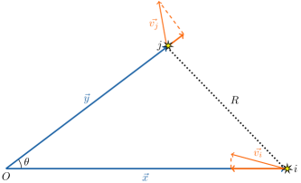
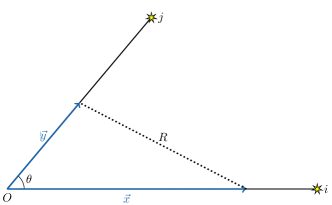
Refer to caption
Refer to caption
Figure 9: Geometrical relations between line-of sight variables for local effects (left), i.e. PV and SW, and integrated ones (right), namely L, TD and ISW.

Peculiar Velocity

As illustrated in Fig. 9, we define x=ηoηi𝑥subscript𝜂𝑜subscript𝜂𝑖x=\eta_{o}-\eta_{i} and y=ηoηj𝑦subscript𝜂𝑜subscript𝜂𝑗y=\eta_{o}-\eta_{j}. Combining Eqs. (14) and (22), for peculiar velocity operator we obtain

𝒲PVij=ΞiΞjGiGjxydΩk4πei𝐤(𝐱𝐲),subscript𝒲𝑃𝑉𝑖𝑗subscriptΞ𝑖subscriptΞ𝑗subscript𝐺𝑖subscript𝐺𝑗subscript𝑥subscript𝑦𝑑subscriptΩ𝑘4𝜋superscript𝑒𝑖𝐤𝐱𝐲\mathcal{W}_{PVij}=\Xi_{i}\Xi_{j}G_{i}G_{j}\partial_{x}\partial_{y}\int\frac{d\Omega_{k}}{4\pi}e^{i{\bf k}\cdot({\bf x}-{\bf y})}\,, (57)

where we have used Eqs. (26). Since 𝐤𝐤{\bf k} has rotational freedom, we align its component along the azimutal axis with 𝐱𝐲𝐱𝐲{\bf x}-{\bf y}, so that the integral over the solid angle becomes

𝑑Ωkei𝐤(𝐱𝐲)=2π11d(cosθk)eikRcosθk=4πj0(kR),differential-dsubscriptΩ𝑘superscript𝑒𝑖𝐤𝐱𝐲2𝜋superscriptsubscript11𝑑subscript𝜃𝑘superscript𝑒𝑖𝑘𝑅subscript𝜃𝑘4𝜋subscript𝑗0𝑘𝑅\int{d\Omega_{k}}e^{i{\bf k}\cdot({\bf x}-{\bf y})}=2\pi\int_{-1}^{1}d\left(\cos\theta_{k}\right)e^{ikR\cos\theta_{k}}=4\pi j_{0}(kR)\,, (58)

where j0subscript𝑗0j_{0} is the 00-th order spherical Bessel function and R=R(x,y,ν)𝑅𝑅𝑥𝑦𝜈R=R(x,y,\nu) is taken as defined in Eqs. (35). Thus we are left with the evaluation of the derivatives of the spherical Bessel function

xyj0(kR)=kx[j0(kR)yR]=k2j0′′(kR)xRyR+kj0(kR)xyR,subscript𝑥subscript𝑦subscript𝑗0𝑘𝑅𝑘subscript𝑥delimited-[]subscriptsuperscript𝑗0𝑘𝑅subscript𝑦𝑅superscript𝑘2subscriptsuperscript𝑗′′0𝑘𝑅subscript𝑥𝑅subscript𝑦𝑅𝑘subscriptsuperscript𝑗0𝑘𝑅subscript𝑥subscript𝑦𝑅\partial_{x}\partial_{y}j_{0}(kR)=\,k\,\partial_{x}\left[j^{\prime}_{0}(kR)\partial_{y}R\right]=k^{2}j^{\prime\prime}_{0}(kR)\partial_{x}R\,\partial_{y}R+k\,j^{\prime}_{0}(kR)\partial_{x}\partial_{y}R\,, (59)

where jn(z)=zjn(z)subscriptsuperscript𝑗𝑛𝑧subscript𝑧subscript𝑗𝑛𝑧j^{\prime}_{n}(z)=\partial_{z}j_{n}(z), jn′′(z)=z2jn(z)subscriptsuperscript𝑗′′𝑛𝑧subscriptsuperscript2𝑧subscript𝑗𝑛𝑧j^{\prime\prime}_{n}(z)=\partial^{2}_{z}j_{n}(z) and so on. Finally, by exploiting the properties of the jnsubscript𝑗𝑛j_{n} reported in Eq. (85), we obtain

𝒲PVijsubscript𝒲𝑃𝑉𝑖𝑗\displaystyle\mathcal{W}_{PVij} =ΞiΞjGiGjk2{xy(1ν2)R2j2(kR)+ν3[j0(kR)2j2(kR)]},absentsubscriptΞ𝑖subscriptΞ𝑗subscript𝐺𝑖subscript𝐺𝑗superscript𝑘2𝑥𝑦1superscript𝜈2superscript𝑅2subscript𝑗2𝑘𝑅𝜈3delimited-[]subscript𝑗0𝑘𝑅2subscript𝑗2𝑘𝑅\displaystyle=\Xi_{i}\Xi_{j}G_{i}G_{j}k^{2}\left\{\frac{xy(1-\nu^{2})}{R^{2}}j_{2}(kR)+\frac{\nu}{3}\left[j_{0}(kR)-2j_{2}(kR)\right]\right\}\,, (60)

in agreement with Ben-Dayan et al. (2014).

Lensing

From right panel of Fig. 9, we define x=ηoη𝑥subscript𝜂𝑜𝜂x=\eta_{o}-\eta and y=ηoη𝑦subscript𝜂𝑜superscript𝜂y=\eta_{o}-\eta^{\prime}. From the definition of the lensing operator in Eqs. (14), we then obtain

𝒲Lij=1ΔηiΔηjηiηo𝑑ηηηiηoηηjηo𝑑ηηηjηoηg(η)g(η)g(ηo2)dΩk4πΔ2xΔ2yei𝐤(𝐱𝐲).subscript𝒲𝐿𝑖𝑗1Δsubscript𝜂𝑖Δsubscript𝜂𝑗superscriptsubscriptsubscript𝜂𝑖subscript𝜂𝑜differential-d𝜂𝜂subscript𝜂𝑖subscript𝜂𝑜𝜂superscriptsubscriptsubscript𝜂𝑗subscript𝜂𝑜differential-dsuperscript𝜂superscript𝜂subscript𝜂𝑗subscript𝜂𝑜superscript𝜂𝑔𝜂𝑔superscript𝜂𝑔superscriptsubscript𝜂𝑜2𝑑subscriptΩ𝑘4𝜋subscriptΔ2𝑥subscriptΔ2𝑦superscript𝑒𝑖𝐤𝐱𝐲\mathcal{W}_{Lij}=\frac{1}{\Delta\eta_{i}\Delta\eta_{j}}\int_{\eta_{i}}^{\eta_{o}}d\eta\frac{\eta-\eta_{i}}{\eta_{o}-\eta}\int_{\eta_{j}}^{\eta_{o}}d\eta^{\prime}\frac{\eta^{\prime}-\eta_{j}}{\eta_{o}-\eta^{\prime}}\frac{g(\eta)g(\eta^{\prime})}{g(\eta_{o}^{2})}\int\frac{d\Omega_{k}}{4\pi}\Delta_{2x}\Delta_{2y}e^{i{\bf k}\cdot({\bf x}-{\bf y})}\,. (61)

We recall now that Δ2r=θ2+cotθθ+1/sin2θϕ2subscriptΔ2𝑟superscriptsubscript𝜃2𝜃subscript𝜃1superscript2𝜃superscriptsubscriptitalic-ϕ2\Delta_{2r}=\partial_{\theta}^{2}+\cot{\theta}\,\partial_{\theta}+1/\sin^{2}{\theta}\,\partial_{\phi}^{2} is the angular Laplacian which can be either evaluated along the r=x𝑟𝑥r=x or r=y𝑟𝑦r=y direction. It can be written in terms of the 3-dimensional one as

Δ2r=r2(r2)=r2(r22rr).subscriptΔ2𝑟superscript𝑟2subscriptsuperscript2𝑟superscript𝑟2superscriptsubscript𝑟22𝑟subscript𝑟\Delta_{2r}=r^{2}\left(\vec{\nabla}\cdot\vec{\nabla}-\nabla^{2}_{r}\right)=r^{2}\left(\vec{\nabla}\cdot\vec{\nabla}-\partial_{r}^{2}-\frac{2}{r}\partial_{r}\right)\,. (62)

We use Eq. (62) to replace the Laplacian in the angular coordinates and get easier evaluable derivatives. With such a substitution, the last integral in Eq. (61) becomes

dΩk4πΔ2Δ2ei𝐤(𝐱𝐲)=𝑑subscriptΩ𝑘4𝜋subscriptΔ2subscriptsuperscriptΔ2superscript𝑒𝑖𝐤𝐱𝐲absent\displaystyle\int\frac{d\Omega_{k}}{4\pi}\Delta_{2}\Delta^{\prime}_{2}e^{i{\bf k}\cdot({\bf x}-{\bf y})}= dΩk4πx2(xxx22xx)y2(yyy22yy)ei𝐤(𝐱𝐲)𝑑subscriptΩ𝑘4𝜋superscript𝑥2subscript𝑥subscript𝑥superscriptsubscript𝑥22𝑥subscript𝑥superscript𝑦2subscript𝑦subscript𝑦superscriptsubscript𝑦22𝑦subscript𝑦superscript𝑒𝑖𝐤𝐱𝐲\displaystyle\int\frac{d\Omega_{k}}{4\pi}x^{2}\left(\vec{\nabla}_{x}\cdot\vec{\nabla}_{x}-\partial_{x}^{2}-\frac{2}{x}\partial_{x}\right)y^{2}\left(\vec{\nabla}_{y}\cdot\vec{\nabla}_{y}-\partial_{y}^{2}-\frac{2}{y}\partial_{y}\right)e^{i{\bf k}\cdot({\bf x}-{\bf y})}
=\displaystyle= dΩk4πx2(k2x22xx)y2(k2y22yy)ei𝐤(𝐱𝐲)𝑑subscriptΩ𝑘4𝜋superscript𝑥2superscript𝑘2superscriptsubscript𝑥22𝑥subscript𝑥superscript𝑦2superscript𝑘2superscriptsubscript𝑦22𝑦subscript𝑦superscript𝑒𝑖𝐤𝐱𝐲\displaystyle\int\frac{d\Omega_{k}}{4\pi}x^{2}\left(-k^{2}-\partial_{x}^{2}-\frac{2}{x}\partial_{x}\right)y^{2}\left(-k^{2}-\partial_{y}^{2}-\frac{2}{y}\partial_{y}\right)e^{i{\bf k}\cdot({\bf x}-{\bf y})}
=\displaystyle= x2(k2x22xx)y2(k2y22yy)j0(kR),superscript𝑥2superscript𝑘2superscriptsubscript𝑥22𝑥subscript𝑥superscript𝑦2superscript𝑘2superscriptsubscript𝑦22𝑦subscript𝑦subscript𝑗0𝑘𝑅\displaystyle x^{2}\left(-k^{2}-\partial_{x}^{2}-\frac{2}{x}\partial_{x}\right)y^{2}\left(-k^{2}-\partial_{y}^{2}-\frac{2}{y}\partial_{y}\right)j_{0}(kR)\,, (63)

where last equality has been obtained thanks to Eq. (58). Hence, by using the recursive relations of the jnsubscript𝑗𝑛j_{n}’s in Eq. (85), after a bit of algebra, 𝒲Lijsubscript𝒲𝐿𝑖𝑗\mathcal{W}_{Lij} can be rewritten as

𝒲Lij=subscript𝒲𝐿𝑖𝑗absent\displaystyle\mathcal{W}_{Lij}= 1Δηi1Δηjηiηodηηηiηoηηjηodηηηjηoηg(η)g(η)g(ηo2)[k4H4j4(kR)\displaystyle\frac{1}{\Delta\eta_{i}}\frac{1}{\Delta\eta_{j}}\int_{\eta_{i}}^{\eta_{o}}d\eta\frac{\eta-\eta_{i}}{\eta_{o}-\eta}\int_{\eta_{j}}^{\eta_{o}}d\eta^{\prime}\frac{\eta^{\prime}-\eta_{j}}{\eta_{o}-\eta^{\prime}}\frac{g(\eta)g(\eta^{\prime})}{g(\eta_{o}^{2})}\left[k^{4}H^{4}j_{4}(kR)\right.
8k3H2Lj3(kR)+k2(8L26H2)j2(kR)+4kLj1(kR)]\displaystyle\left.-8k^{3}H^{2}Lj_{3}(kR)+k^{2}\left(8L^{2}-6H^{2}\right)j_{2}(kR)+4kLj_{1}(kR)\right] (64)

where H𝐻H, L and R𝑅R are defined in Eqs. (35).

Sachs-Wolfe

In analogy with what has been done for the peculiar velocity, we refer to left panel of Fig. 9, we define x=ηoηi𝑥subscript𝜂𝑜subscript𝜂𝑖x=\eta_{o}-\eta_{i} and y=ηoηj𝑦subscript𝜂𝑜subscript𝜂𝑗y=\eta_{o}-\eta_{j} and consider the operator 𝒪^SWsubscript^𝒪𝑆𝑊\hat{\mathcal{O}}_{SW} in Eqs. (14). Since no spatial derivatives are considered, we simply get, though Eq. (58)

𝒲SWij=subscript𝒲𝑆𝑊𝑖𝑗absent\displaystyle\mathcal{W}_{SWij}= (1+Ξi)(1+Ξj)g(ηi)g(ηo)g(ηj)g(ηo)dΩk4πei𝐤(𝐱𝐲)1subscriptΞ𝑖1subscriptΞ𝑗𝑔subscript𝜂𝑖𝑔subscript𝜂𝑜𝑔subscript𝜂𝑗𝑔subscript𝜂𝑜𝑑subscriptΩ𝑘4𝜋superscript𝑒𝑖𝐤𝐱𝐲\displaystyle(1+\Xi_{i})(1+\Xi_{j})\,\frac{g(\eta_{i})}{g(\eta_{o})}\frac{g(\eta_{j})}{g(\eta_{o})}\int\frac{d\Omega_{k}}{4\pi}e^{i{\bf k}\cdot\left({\bf x}-{\bf y}\right)}
=\displaystyle= (1+Ξi)(1+Ξj)g(ηi)g(ηo)g(ηj)g(ηo)j0(kR),1subscriptΞ𝑖1subscriptΞ𝑗𝑔subscript𝜂𝑖𝑔subscript𝜂𝑜𝑔subscript𝜂𝑗𝑔subscript𝜂𝑜subscript𝑗0𝑘𝑅\displaystyle(1+\Xi_{i})(1+\Xi_{j})\,\frac{g(\eta_{i})}{g(\eta_{o})}\frac{g(\eta_{j})}{g(\eta_{o})}j_{0}(kR)\,, (65)

where R=R(ηi,ηj,ν)𝑅𝑅subscript𝜂𝑖subscript𝜂𝑗𝜈R=R(\eta_{i},\eta_{j},\nu) is taken from Eqs. (26).

Integrated Sachs-Wolfe

In analogy with the geometrical set used for lensing (right panel in Fig. 9), we define x=ηoη𝑥subscript𝜂𝑜𝜂x=\eta_{o}-\eta and y=χ=ηoη𝑦superscript𝜒subscript𝜂𝑜superscript𝜂y=\chi^{\prime}=\eta_{o}-\eta^{\prime}. Given that we simply obtain

𝒲ISWij=subscript𝒲𝐼𝑆𝑊𝑖𝑗absent\displaystyle\mathcal{W}_{ISWij}= 4ΞiΞjηiηo𝑑ηηjηo𝑑ηηg(η)g(ηo)ηg(η)g(ηo)dΩk4πei𝐤(𝐱𝐲)4subscriptΞ𝑖subscriptΞ𝑗superscriptsubscriptsubscript𝜂𝑖subscript𝜂𝑜differential-d𝜂superscriptsubscriptsubscript𝜂𝑗subscript𝜂𝑜differential-dsuperscript𝜂subscript𝜂𝑔𝜂𝑔subscript𝜂𝑜subscriptsuperscript𝜂𝑔superscript𝜂𝑔subscript𝜂𝑜𝑑subscriptΩ𝑘4𝜋superscript𝑒𝑖𝐤𝐱𝐲\displaystyle 4\,\Xi_{i}\Xi_{j}\int_{\eta_{i}}^{\eta_{o}}d\eta\int_{\eta_{j}}^{\eta_{o}}d\eta^{\prime}\frac{\partial_{\eta}g(\eta)}{g(\eta_{o})}\frac{\partial_{\eta^{\prime}}g(\eta^{\prime})}{g(\eta_{o})}\int\frac{d\Omega_{k}}{4\pi}e^{i{\bf k}\cdot\left({\bf x}-{\bf y}\right)}
=\displaystyle= 4ΞiΞjηiηo𝑑ηηjηo𝑑ηηg(η)g(ηo)ηg(η)g(ηo)j0(kR),4subscriptΞ𝑖subscriptΞ𝑗superscriptsubscriptsubscript𝜂𝑖subscript𝜂𝑜differential-d𝜂superscriptsubscriptsubscript𝜂𝑗subscript𝜂𝑜differential-dsuperscript𝜂subscript𝜂𝑔𝜂𝑔subscript𝜂𝑜subscriptsuperscript𝜂𝑔superscript𝜂𝑔subscript𝜂𝑜subscript𝑗0𝑘𝑅\displaystyle 4\Xi_{i}\Xi_{j}\int_{\eta_{i}}^{\eta_{o}}d\eta\int_{\eta_{j}}^{\eta_{o}}d\eta^{\prime}\frac{\partial_{\eta}g(\eta)}{g(\eta_{o})}\frac{\partial_{\eta^{\prime}}g(\eta^{\prime})}{g(\eta_{o})}j_{0}(kR)\,, (66)

where we have used again Eq. (58). We stress that now R=R(η,η,ν)𝑅𝑅𝜂superscript𝜂𝜈R=R(\eta,\eta^{\prime},\nu) from Eqs. (26) is integrated along the two line-of-sights, differently from the case of PV and SW.

Time Delay

TD term can be evaluated in complete analogy with ISW. The only difference is that the growth functions are not derived. Following then the evaluation for ISW, we get

𝒲TDij=4ΔηiΔηjηiηo𝑑ηηjηo𝑑ηg(η)g(ηo)g(η)g(ηo)j0(kR).subscript𝒲𝑇𝐷𝑖𝑗4Δsubscript𝜂𝑖Δsubscript𝜂𝑗superscriptsubscriptsubscript𝜂𝑖subscript𝜂𝑜differential-d𝜂superscriptsubscriptsubscript𝜂𝑗subscript𝜂𝑜differential-dsuperscript𝜂𝑔𝜂𝑔subscript𝜂𝑜𝑔superscript𝜂𝑔subscript𝜂𝑜subscript𝑗0𝑘𝑅\mathcal{W}_{TDij}=\frac{4}{\Delta\eta_{i}\Delta\eta_{j}}\int_{\eta_{i}}^{\eta_{o}}d\eta\int_{\eta_{j}}^{\eta_{o}}d\eta^{\prime}\frac{g(\eta)}{g(\eta_{o})}\frac{g(\eta^{\prime})}{g(\eta_{o})}j_{0}(kR)\,. (67)

There are then 10 mixed terms that come out of the sum in Eq. (20) when EE𝐸superscript𝐸E\neq E^{\prime}. As done for the pure terms, we will use the auxiliary variables x,y𝑥𝑦x,y, whose definitions will be given for each term and differ whether the effect is local or integrated along the line-of-sight. To our aim, we first report the following useful expressions

dΩk4πxei𝐤(𝐱𝐲)=𝑑subscriptΩ𝑘4𝜋subscript𝑥superscript𝑒𝑖𝐤𝐱𝐲absent\displaystyle\int\frac{d\Omega_{k}}{4\pi}\partial_{x}e^{i{\bf k}\cdot({\bf x}-{\bf y})}= kνyxRj1(kR),𝑘𝜈𝑦𝑥𝑅subscript𝑗1𝑘𝑅\displaystyle k\frac{\nu y-x}{R}j_{1}(kR)\,,
dΩk4πΔ2xei𝐤(𝐱𝐲)=𝑑subscriptΩ𝑘4𝜋subscriptΔ2𝑥superscript𝑒𝑖𝐤𝐱𝐲absent\displaystyle\int\frac{d\Omega_{k}}{4\pi}\Delta_{2x}e^{i{\bf k}\cdot({\bf x}-{\bf y})}= k2H2j0(kR)k(3H2R2L)j1(kR),superscript𝑘2superscript𝐻2subscript𝑗0𝑘𝑅𝑘3superscript𝐻2𝑅2𝐿subscript𝑗1𝑘𝑅\displaystyle k^{2}H^{2}j_{0}(kR)-k\left(\frac{3H^{2}}{R}-2L\right)j_{1}(kR)\,,
dΩk4πxΔ2yei𝐤(𝐱𝐲)=𝑑subscriptΩ𝑘4𝜋subscript𝑥subscriptΔ2𝑦superscript𝑒𝑖𝐤𝐱𝐲absent\displaystyle\int\frac{d\Omega_{k}}{4\pi}\partial_{x}\Delta_{2y}e^{i{\bf k}\cdot({\bf x}-{\bf y})}= k3y2(xνy)(yνx)2R3j3(kR)+k2y[3y(xνy)R22ν]j2(kR)superscript𝑘3superscript𝑦2𝑥𝜈𝑦superscript𝑦𝜈𝑥2superscript𝑅3subscript𝑗3𝑘𝑅superscript𝑘2𝑦delimited-[]3𝑦𝑥𝜈𝑦superscript𝑅22𝜈subscript𝑗2𝑘𝑅\displaystyle-k^{3}y^{2}\frac{(x-\nu y)(y-\nu x)^{2}}{R^{3}}j_{3}(kR)+k^{2}y\left[3y\frac{(x-\nu y)}{R^{2}}-2\nu\right]j_{2}(kR)
kyR[k2y(xνy)2ν]j1(kR).𝑘𝑦𝑅delimited-[]superscript𝑘2𝑦𝑥𝜈𝑦2𝜈subscript𝑗1𝑘𝑅\displaystyle-\frac{ky}{R}\left[k^{2}y(x-\nu y)-2\nu\right]j_{1}(kR)\,. (68)

where R𝑅R, L𝐿L and H𝐻H are taken from Eqs. (35).

Peculiar Velocity - Lensing

From the definition of the operators in Eqs. (14), we define x=ηoηi𝑥subscript𝜂𝑜subscript𝜂𝑖x=\eta_{o}-\eta_{i} and y=ηoη𝑦subscript𝜂𝑜superscript𝜂y=\eta_{o}-\eta^{\prime}, since PV is a local effect whereas L is integrated along the line-of-sight. With this, we get

𝒲PVi,Lj=ΞiΔηjηinηi𝑑ηa(η)a(ηo)g(η)g(ηo)ηjηo𝑑ηηηjηoηdΩk4πg(η)g(ηo)xΔ2yei𝐤(𝐱𝐲).subscript𝒲𝑃𝑉𝑖𝐿𝑗subscriptΞ𝑖Δsubscript𝜂𝑗superscriptsubscriptsubscript𝜂𝑖𝑛subscript𝜂𝑖differential-d𝜂𝑎𝜂𝑎subscript𝜂𝑜𝑔𝜂𝑔subscript𝜂𝑜superscriptsubscriptsubscript𝜂𝑗subscript𝜂𝑜differential-dsuperscript𝜂superscript𝜂subscript𝜂𝑗subscript𝜂𝑜superscript𝜂𝑑subscriptΩ𝑘4𝜋𝑔superscript𝜂𝑔subscript𝜂𝑜subscript𝑥subscriptΔ2𝑦superscript𝑒𝑖𝐤𝐱𝐲\mathcal{W}_{PVi,Lj}=\frac{\Xi_{i}}{\Delta\eta_{j}}\int_{\eta_{in}}^{\eta_{i}}d\eta\frac{a(\eta)}{a(\eta_{o})}\frac{g(\eta)}{g(\eta_{o})}\int_{\eta_{j}}^{\eta_{o}}d\eta^{\prime}\frac{\eta^{\prime}-\eta_{j}}{\eta_{o}-\eta^{\prime}}\int\frac{d\Omega_{k}}{4\pi}\frac{g(\eta^{\prime})}{g(\eta_{o})}\partial_{x}\Delta_{2y}e^{i{\bf k}\cdot({\bf x}-{\bf y})}\,. (69)

Hence, by using Eqs. (68), we obtain

𝒲PVi,Lj=subscript𝒲𝑃𝑉𝑖𝐿𝑗absent\displaystyle\mathcal{W}_{PVi,Lj}= ΞiΔηjGiηjηodηηηjηoη{k3y2(xνy)(yνx)2R3j3+k2y[3y(xνy)R22ν]j2\displaystyle\frac{\Xi_{i}}{\Delta\eta_{j}}G_{i}\int_{\eta_{j}}^{\eta_{o}}d\eta^{\prime}\frac{\eta^{\prime}-\eta_{j}}{\eta_{o}-\eta^{\prime}}\left\{-k^{3}y^{2}\frac{(x-\nu y)(y-\nu x)^{2}}{R^{3}}j_{3}+k^{2}y\left[3y\frac{(x-\nu y)}{R^{2}}-2\nu\right]j_{2}\right.
kyR[k2y(xνy)2ν]j1},\displaystyle\left.-\frac{ky}{R}\left[k^{2}y(x-\nu y)-2\nu\right]j_{1}\right\}\,, (70)

where we have omitted the dependence on kR(x,y,ν)𝑘𝑅𝑥𝑦𝜈kR(x,y,\nu) in the jnsubscript𝑗𝑛j_{n}’s.

Peculiar Velocity - Sachs-Wolfe

Since both effects are local effects, we define x=ηoηi𝑥subscript𝜂𝑜subscript𝜂𝑖x=\eta_{o}-\eta_{i} and y=ηoηj𝑦subscript𝜂𝑜subscript𝜂𝑗y=\eta_{o}-\eta_{j}. From the definitions of the respective operators in Eqs. (14), we find

𝒲PVi,SWj=subscript𝒲𝑃𝑉𝑖𝑆𝑊𝑗absent\displaystyle\mathcal{W}_{PVi,SWj}= Ξi(1+Ξj)ηinηi𝑑ηa(η)a(ηo)g(η)g(ηo)g(ηj)g(ηo)dΩk4πxei𝐤(𝐱𝐲)subscriptΞ𝑖1subscriptΞ𝑗superscriptsubscriptsubscript𝜂𝑖𝑛subscript𝜂𝑖differential-d𝜂𝑎𝜂𝑎subscript𝜂𝑜𝑔𝜂𝑔subscript𝜂𝑜𝑔subscript𝜂𝑗𝑔subscript𝜂𝑜𝑑subscriptΩ𝑘4𝜋subscript𝑥superscript𝑒𝑖𝐤𝐱𝐲\displaystyle\Xi_{i}(1+\Xi_{j})\int_{\eta_{in}}^{\eta_{i}}d\eta\frac{a(\eta)}{a(\eta_{o})}\frac{g(\eta)}{g(\eta_{o})}\frac{g(\eta_{j})}{g(\eta_{o})}\int\frac{d\Omega_{k}}{4\pi}\partial_{x}e^{i{\bf k}\cdot({\bf x}-{\bf y})}
=\displaystyle= Ξi(1+Ξj)Gig(ηj)g(ηo)kνyxRj1(kR),subscriptΞ𝑖1subscriptΞ𝑗subscript𝐺𝑖𝑔subscript𝜂𝑗𝑔subscript𝜂𝑜𝑘𝜈𝑦𝑥𝑅subscript𝑗1𝑘𝑅\displaystyle\Xi_{i}(1+\Xi_{j})G_{i}\frac{g(\eta_{j})}{g(\eta_{o})}\,k\,\frac{\nu y-x}{R}j_{1}(kR)\,, (71)

where we made use again of Eqs. (68).

Peculiar Velocity - Integrated Sachs-Wolfe

Since PV is a local effect whereas ISW is integrated along the line-of-sight, we define x=ηoηi𝑥subscript𝜂𝑜subscript𝜂𝑖x=\eta_{o}-\eta_{i} and y=ηoη𝑦subscript𝜂𝑜superscript𝜂y=\eta_{o}-\eta^{\prime}. Hence, from the definitions of the operators in Eqs. (14), we get

𝒲PVi,ISWj=subscript𝒲𝑃𝑉𝑖𝐼𝑆𝑊𝑗absent\displaystyle\mathcal{W}_{PVi,ISWj}= 2ΞiΞjηinηi𝑑ηa(η)a(ηo)g(η)g(ηo)ηjηo𝑑ηηg(η)g(ηo)dΩk4πxei𝐤(𝐱𝐲)2subscriptΞ𝑖subscriptΞ𝑗superscriptsubscriptsubscript𝜂𝑖𝑛subscript𝜂𝑖differential-d𝜂𝑎𝜂𝑎subscript𝜂𝑜𝑔𝜂𝑔subscript𝜂𝑜superscriptsubscriptsubscript𝜂𝑗subscript𝜂𝑜differential-dsuperscript𝜂subscriptsuperscript𝜂𝑔superscript𝜂𝑔subscript𝜂𝑜𝑑subscriptΩ𝑘4𝜋subscript𝑥superscript𝑒𝑖𝐤𝐱𝐲\displaystyle 2\,\Xi_{i}\Xi_{j}\int_{\eta_{in}}^{\eta_{i}}d\eta\frac{a(\eta)}{a(\eta_{o})}\frac{g(\eta)}{g(\eta_{o})}\int_{\eta_{j}}^{\eta_{o}}d\eta^{\prime}\frac{\partial_{\eta^{\prime}}g(\eta^{\prime})}{g(\eta_{o})}\int\frac{d\Omega_{k}}{4\pi}\partial_{x}e^{i{\bf k}\cdot({\bf x}-{\bf y})}
=\displaystyle= 2ΞiΞjGiηjηo𝑑ηηg(η)g(ηo)kνyxRj1(kR),2subscriptΞ𝑖subscriptΞ𝑗subscript𝐺𝑖superscriptsubscriptsubscript𝜂𝑗subscript𝜂𝑜differential-dsuperscript𝜂subscriptsuperscript𝜂𝑔superscript𝜂𝑔subscript𝜂𝑜𝑘𝜈𝑦𝑥𝑅subscript𝑗1𝑘𝑅\displaystyle 2\,\Xi_{i}\Xi_{j}G_{i}\int_{\eta_{j}}^{\eta_{o}}d\eta^{\prime}\frac{\partial_{\eta^{\prime}}g(\eta^{\prime})}{g(\eta_{o})}\,k\,\frac{\nu y-x}{R}j_{1}(kR)\,, (72)

where we have used as before Eqs. (68).

Peculiar Velocity - Time Delay

Since PV is a local effect whereas TD is integrated along the line-of-sight, we define x=ηoηi𝑥subscript𝜂𝑜subscript𝜂𝑖x=\eta_{o}-\eta_{i} and y=ηoη𝑦subscript𝜂𝑜superscript𝜂y=\eta_{o}-\eta^{\prime}. Hence, from the definitions of the operators in Eqs. (14), we obtain

𝒲PVi,TDj=subscript𝒲𝑃𝑉𝑖𝑇𝐷𝑗absent\displaystyle\mathcal{W}_{PVi,TDj}= 2ΞiΔηjηinηi𝑑ηa(η)a(ηo)g(η)g(ηo)ηjηo𝑑ηg(η)g(ηo)dΩk4πxei𝐤(𝐱𝐲)2subscriptΞ𝑖Δsubscript𝜂𝑗superscriptsubscriptsubscript𝜂𝑖𝑛subscript𝜂𝑖differential-d𝜂𝑎𝜂𝑎subscript𝜂𝑜𝑔𝜂𝑔subscript𝜂𝑜superscriptsubscriptsubscript𝜂𝑗subscript𝜂𝑜differential-dsuperscript𝜂𝑔superscript𝜂𝑔subscript𝜂𝑜𝑑subscriptΩ𝑘4𝜋subscript𝑥superscript𝑒𝑖𝐤𝐱𝐲\displaystyle-2\,\frac{\Xi_{i}}{\Delta\eta_{j}}\int_{\eta_{in}}^{\eta_{i}}d\eta\frac{a(\eta)}{a(\eta_{o})}\frac{g(\eta)}{g(\eta_{o})}\int_{\eta_{j}}^{\eta_{o}}d\eta^{\prime}\frac{g(\eta^{\prime})}{g(\eta_{o})}\int\frac{d\Omega_{k}}{4\pi}\partial_{x}e^{i{\bf k}\cdot({\bf x}-{\bf y})}
=\displaystyle= 2ΞiΔηjGiηjηo𝑑ηg(η)g(ηo)kνyxRj1(kR)2subscriptΞ𝑖Δsubscript𝜂𝑗subscript𝐺𝑖superscriptsubscriptsubscript𝜂𝑗subscript𝜂𝑜differential-dsuperscript𝜂𝑔superscript𝜂𝑔subscript𝜂𝑜𝑘𝜈𝑦𝑥𝑅subscript𝑗1𝑘𝑅\displaystyle-2\,\frac{\Xi_{i}}{\Delta\eta_{j}}G_{i}\int_{\eta_{j}}^{\eta_{o}}d\eta^{\prime}\frac{g(\eta^{\prime})}{g(\eta_{o})}\,k\,\frac{\nu y-x}{R}j_{1}(kR) (73)

where we have used as before Eqs. (68).

Lensing - Sachs-Wolfe

Since L is an integrated effect and SW is a local one, we set the geometrical variables as x=ηoη𝑥subscript𝜂𝑜𝜂x=\eta_{o}-\eta and y=ηoηj𝑦subscript𝜂𝑜subscript𝜂𝑗y=\eta_{o}-\eta_{j}. Hence, the definition of the operators in Eqs. (14) leads to

𝒲Li,SWj=subscript𝒲𝐿𝑖𝑆𝑊𝑗absent\displaystyle\mathcal{W}_{Li,SWj}= 1+ΞjΔηig(ηj)g(ηo)ηiηo𝑑ηηηjηoηg(η)g(ηo)dΩk4πΔ2yei𝐤(𝐱𝐲)1subscriptΞ𝑗Δsubscript𝜂𝑖𝑔subscript𝜂𝑗𝑔subscript𝜂𝑜superscriptsubscriptsubscript𝜂𝑖subscript𝜂𝑜differential-d𝜂𝜂subscript𝜂𝑗subscript𝜂𝑜𝜂𝑔𝜂𝑔subscript𝜂𝑜𝑑subscriptΩ𝑘4𝜋subscriptΔ2𝑦superscript𝑒𝑖𝐤𝐱𝐲\displaystyle\frac{1+\Xi_{j}}{\Delta\eta_{i}}\frac{g(\eta_{j})}{g(\eta_{o})}\int_{\eta_{i}}^{\eta_{o}}d\eta\frac{\eta-\eta_{j}}{\eta_{o}-\eta}\frac{g(\eta)}{g(\eta_{o})}\int\frac{d\Omega_{k}}{4\pi}\Delta_{2y}e^{i{\bf k}\cdot({\bf x}-{\bf y})}
=\displaystyle= 1+ΞjΔηig(ηj)g(ηo)ηiηo𝑑ηηηjηoηg(η)g(ηo)[k2H2j0(kR)k(3H2R2L)j1(kR)],1subscriptΞ𝑗Δsubscript𝜂𝑖𝑔subscript𝜂𝑗𝑔subscript𝜂𝑜superscriptsubscriptsubscript𝜂𝑖subscript𝜂𝑜differential-d𝜂𝜂subscript𝜂𝑗subscript𝜂𝑜𝜂𝑔𝜂𝑔subscript𝜂𝑜delimited-[]superscript𝑘2superscript𝐻2subscript𝑗0𝑘𝑅𝑘3superscript𝐻2𝑅2𝐿subscript𝑗1𝑘𝑅\displaystyle\frac{1+\Xi_{j}}{\Delta\eta_{i}}\frac{g(\eta_{j})}{g(\eta_{o})}\int_{\eta_{i}}^{\eta_{o}}d\eta\frac{\eta-\eta_{j}}{\eta_{o}-\eta}\frac{g(\eta)}{g(\eta_{o})}\left[k^{2}H^{2}j_{0}(kR)-k\left(\frac{3H^{2}}{R}-2L\right)j_{1}(kR)\right]\,, (74)

thanks to the Eqs. (68).

Lensing - Integral Sachs Wolfe

Since both effects are integrated along the line-of-sights, we define x=ηoη𝑥subscript𝜂𝑜𝜂x=\eta_{o}-\eta and y=ηoη𝑦subscript𝜂𝑜superscript𝜂y=\eta_{o}-\eta^{\prime}. Hence, the action of the operators (14), combined with Eqs. (68), gives

𝒲Li,ISWj=subscript𝒲𝐿𝑖𝐼𝑆𝑊𝑗absent\displaystyle\mathcal{W}_{Li,ISWj}= 2ΞjΔηiηiηo𝑑ηηηjηoηg(η)g(ηo)ηjηo𝑑ηηg(η)g(ηo)dΩk4πΔ2yei𝐤(𝐱𝐲)2subscriptΞ𝑗Δsubscript𝜂𝑖superscriptsubscriptsubscript𝜂𝑖subscript𝜂𝑜differential-d𝜂𝜂subscript𝜂𝑗subscript𝜂𝑜𝜂𝑔𝜂𝑔subscript𝜂𝑜superscriptsubscriptsubscript𝜂𝑗subscript𝜂𝑜differential-dsuperscript𝜂subscriptsuperscript𝜂𝑔superscript𝜂𝑔subscript𝜂𝑜𝑑subscriptΩ𝑘4𝜋subscriptΔ2𝑦superscript𝑒𝑖𝐤𝐱𝐲\displaystyle 2\,\frac{\Xi_{j}}{\Delta\eta_{i}}\int_{\eta_{i}}^{\eta_{o}}d\eta\frac{\eta-\eta_{j}}{\eta_{o}-\eta}\frac{g(\eta)}{g(\eta_{o})}\int_{\eta_{j}}^{\eta_{o}}d\eta^{\prime}\frac{\partial_{\eta^{\prime}}g(\eta^{\prime})}{g(\eta_{o})}\int\frac{d\Omega_{k}}{4\pi}\Delta_{2y}e^{i{\bf k}\cdot({\bf x}-{\bf y})}
=\displaystyle= 2ΞjΔηiηiηo𝑑ηηηjηoηg(η)g(ηo)ηjηo𝑑ηηg(η)g(ηo)[k2H2j0(kR)k(3H2R2L)j1(kR)].2subscriptΞ𝑗Δsubscript𝜂𝑖superscriptsubscriptsubscript𝜂𝑖subscript𝜂𝑜differential-d𝜂𝜂subscript𝜂𝑗subscript𝜂𝑜𝜂𝑔𝜂𝑔subscript𝜂𝑜superscriptsubscriptsubscript𝜂𝑗subscript𝜂𝑜differential-dsuperscript𝜂subscriptsuperscript𝜂𝑔superscript𝜂𝑔subscript𝜂𝑜delimited-[]superscript𝑘2superscript𝐻2subscript𝑗0𝑘𝑅𝑘3superscript𝐻2𝑅2𝐿subscript𝑗1𝑘𝑅\displaystyle 2\,\frac{\Xi_{j}}{\Delta\eta_{i}}\int_{\eta_{i}}^{\eta_{o}}d\eta\frac{\eta-\eta_{j}}{\eta_{o}-\eta}\frac{g(\eta)}{g(\eta_{o})}\int_{\eta_{j}}^{\eta_{o}}d\eta^{\prime}\frac{\partial_{\eta^{\prime}}g(\eta^{\prime})}{g(\eta_{o})}\left[k^{2}H^{2}j_{0}(kR)-k\left(\frac{3H^{2}}{R}-2L\right)j_{1}(kR)\right]\,. (75)

Lensing - Time Delay

Since L and TD are both integrated along the line-of-sights, we define x=ηoη𝑥subscript𝜂𝑜𝜂x=\eta_{o}-\eta and y=ηoη𝑦subscript𝜂𝑜superscript𝜂y=\eta_{o}-\eta^{\prime}, so, with the definition (14), we simply evaluate

𝒲Li,TDj=21ΔηiΔηjηiηosubscript𝒲𝐿𝑖𝑇𝐷𝑗21Δsubscript𝜂𝑖Δsubscript𝜂𝑗superscriptsubscriptsubscript𝜂𝑖subscript𝜂𝑜\displaystyle\mathcal{W}_{Li,TDj}=-2\,\frac{1}{\Delta\eta_{i}\Delta\eta_{j}}\int_{\eta_{i}}^{\eta_{o}} dηηηjηoηg(η)g(ηo)ηjηo𝑑ηg(η)g(ηo)dΩk4πΔ2yei𝐤(𝐱𝐲)𝑑𝜂𝜂subscript𝜂𝑗subscript𝜂𝑜𝜂𝑔𝜂𝑔subscript𝜂𝑜superscriptsubscriptsubscript𝜂𝑗subscript𝜂𝑜differential-dsuperscript𝜂𝑔superscript𝜂𝑔subscript𝜂𝑜𝑑subscriptΩ𝑘4𝜋subscriptΔ2𝑦superscript𝑒𝑖𝐤𝐱𝐲\displaystyle d\eta\frac{\eta-\eta_{j}}{\eta_{o}-\eta}\frac{g(\eta)}{g(\eta_{o})}\int_{\eta_{j}}^{\eta_{o}}d\eta^{\prime}\frac{g(\eta^{\prime})}{g(\eta_{o})}\int\frac{d\Omega_{k}}{4\pi}\Delta_{2y}e^{i{\bf k}\cdot({\bf x}-{\bf y})}
=\displaystyle= 21ΔηiΔηiηiηo𝑑ηηηjηoηg(η)g(ηo)ηjηo𝑑ηg(η)g(ηo)[k2H2j0(kR)k(3H2R2L)j1(kR)],21Δsubscript𝜂𝑖Δsubscript𝜂𝑖superscriptsubscriptsubscript𝜂𝑖subscript𝜂𝑜differential-d𝜂𝜂subscript𝜂𝑗subscript𝜂𝑜𝜂𝑔𝜂𝑔subscript𝜂𝑜superscriptsubscriptsubscript𝜂𝑗subscript𝜂𝑜differential-dsuperscript𝜂𝑔superscript𝜂𝑔subscript𝜂𝑜delimited-[]superscript𝑘2superscript𝐻2subscript𝑗0𝑘𝑅𝑘3superscript𝐻2𝑅2𝐿subscript𝑗1𝑘𝑅\displaystyle-2\,\frac{1}{\Delta\eta_{i}\Delta\eta_{i}}\int_{\eta_{i}}^{\eta_{o}}d\eta\frac{\eta-\eta_{j}}{\eta_{o}-\eta}\frac{g(\eta)}{g(\eta_{o})}\int_{\eta_{j}}^{\eta_{o}}d\eta^{\prime}\frac{g(\eta^{\prime})}{g(\eta_{o})}\left[k^{2}H^{2}j_{0}(kR)-k\left(\frac{3H^{2}}{R}-2L\right)j_{1}(kR)\right]\,, (76)

thanks to the relations (68).

Time Delay - Integrated Sachs-Wolfe

Just as for the previous term, we define x=ηoη𝑥subscript𝜂𝑜𝜂x=\eta_{o}-\eta and y=ηoη𝑦subscript𝜂𝑜superscript𝜂y=\eta_{o}-\eta^{\prime} since both TD and ISW are integrated effects. Hence, from the operators defined in Eqs. (14), we obtain

𝒲TDi,ISWj=subscript𝒲𝑇𝐷𝑖𝐼𝑆𝑊𝑗absent\displaystyle\mathcal{W}_{TDi,ISWj}= 2(1+Ξi)Ξjg(ηi)g(ηo)ηjηo𝑑ηηg(η)g(ηo)dΩk4πei𝐤(𝐱𝐲)21subscriptΞ𝑖subscriptΞ𝑗𝑔subscript𝜂𝑖𝑔subscript𝜂𝑜superscriptsubscriptsubscript𝜂𝑗subscript𝜂𝑜differential-dsuperscript𝜂subscriptsuperscript𝜂𝑔superscript𝜂𝑔subscript𝜂𝑜𝑑subscriptΩ𝑘4𝜋superscript𝑒𝑖𝐤𝐱𝐲\displaystyle 2\,(1+\Xi_{i})\Xi_{j}\frac{g(\eta_{i})}{g(\eta_{o})}\int_{\eta_{j}}^{\eta_{o}}d\eta^{\prime}\frac{\partial_{\eta^{\prime}}g(\eta^{\prime})}{g(\eta_{o})}\int\frac{d\Omega_{k}}{4\pi}e^{i{\bf k}\cdot({\bf x}-{\bf y})}
=\displaystyle= 2(1+Ξi)Ξjg(ηi)g(ηo)ηjηo𝑑ηηg(η)g(ηo)j0(kR),21subscriptΞ𝑖subscriptΞ𝑗𝑔subscript𝜂𝑖𝑔subscript𝜂𝑜superscriptsubscriptsubscript𝜂𝑗subscript𝜂𝑜differential-dsuperscript𝜂subscriptsuperscript𝜂𝑔superscript𝜂𝑔subscript𝜂𝑜subscript𝑗0𝑘𝑅\displaystyle 2\,(1+\Xi_{i})\Xi_{j}\frac{g(\eta_{i})}{g(\eta_{o})}\int_{\eta_{j}}^{\eta_{o}}d\eta^{\prime}\frac{\partial_{\eta^{\prime}}g(\eta^{\prime})}{g(\eta_{o})}\,j_{0}(kR)\,, (77)

where we have applied Eq. (58).

Sachs-Wolfe - Time Delay

SW and TD are respectively local and integrated effects. Because of that, we define x=ηoηi𝑥subscript𝜂𝑜subscript𝜂𝑖x=\eta_{o}-\eta_{i} and y=ηoη𝑦subscript𝜂𝑜superscript𝜂y=\eta_{o}-\eta^{\prime} and then, from the operators (14), we obtain

𝒲SWi,TDj=21+ΞiΔηjg(ηi)g(ηo)ηjηo𝑑ηg(η)g(ηo)dΩk4πei𝐤(𝐱𝐲)=21+ΞiΔηjg(ηi)g(ηo)ηjηo𝑑ηg(η)g(ηo)j0(kR),subscript𝒲𝑆𝑊𝑖𝑇𝐷𝑗21subscriptΞ𝑖Δsubscript𝜂𝑗𝑔subscript𝜂𝑖𝑔subscript𝜂𝑜superscriptsubscriptsubscript𝜂𝑗subscript𝜂𝑜differential-dsuperscript𝜂𝑔superscript𝜂𝑔subscript𝜂𝑜𝑑subscriptΩ𝑘4𝜋superscript𝑒𝑖𝐤𝐱𝐲21subscriptΞ𝑖Δsubscript𝜂𝑗𝑔subscript𝜂𝑖𝑔subscript𝜂𝑜superscriptsubscriptsubscript𝜂𝑗subscript𝜂𝑜differential-dsuperscript𝜂𝑔superscript𝜂𝑔subscript𝜂𝑜subscript𝑗0𝑘𝑅\mathcal{W}_{SWi,TDj}=-2\,\frac{1+\Xi_{i}}{\Delta\eta_{j}}\frac{g(\eta_{i})}{g(\eta_{o})}\int_{\eta_{j}}^{\eta_{o}}d\eta^{\prime}\frac{g(\eta^{\prime})}{g(\eta_{o})}\int\frac{d\Omega_{k}}{4\pi}e^{i{\bf k}\cdot({\bf x}-{\bf y})}=-2\,\frac{1+\Xi_{i}}{\Delta\eta_{j}}\frac{g(\eta_{i})}{g(\eta_{o})}\int_{\eta_{j}}^{\eta_{o}}d\eta^{\prime}\frac{g(\eta^{\prime})}{g(\eta_{o})}\,j_{0}(kR)\,, (78)

where we have applied Eq. (58).

Integrated Sachs-Wolfe - Time Delay

ISW and TD are both integrated effects. Hence, we define x=ηoη𝑥subscript𝜂𝑜𝜂x=\eta_{o}-\eta and y=ηoη𝑦subscript𝜂𝑜superscript𝜂y=\eta_{o}-\eta^{\prime} and then, from the operators (14), we obtain

𝒲ISWi,TDj=subscript𝒲𝐼𝑆𝑊𝑖𝑇𝐷𝑗absent\displaystyle\mathcal{W}_{ISWi,TDj}= 4ΞiΔηjηiηo𝑑ηηg(η)g(ηo)ηjηo𝑑ηg(η)g(ηo)dΩk4πei𝐤(𝐱𝐲)4subscriptΞ𝑖Δsubscript𝜂𝑗superscriptsubscriptsubscript𝜂𝑖subscript𝜂𝑜differential-d𝜂subscript𝜂𝑔𝜂𝑔subscript𝜂𝑜superscriptsubscriptsubscript𝜂𝑗subscript𝜂𝑜differential-dsuperscript𝜂𝑔superscript𝜂𝑔subscript𝜂𝑜𝑑subscriptΩ𝑘4𝜋superscript𝑒𝑖𝐤𝐱𝐲\displaystyle-4\,\frac{\Xi_{i}}{\Delta\eta_{j}}\int_{\eta_{i}}^{\eta_{o}}d\eta\frac{\partial_{\eta}g(\eta)}{g(\eta_{o})}\int_{\eta_{j}}^{\eta_{o}}d\eta^{\prime}\frac{g(\eta^{\prime})}{g(\eta_{o})}\int\frac{d\Omega_{k}}{4\pi}e^{i{\bf k}\cdot({\bf x}-{\bf y})}
=\displaystyle= 4ΞiΔηjηiηo𝑑ηηg(η)g(ηo)ηjηo𝑑ηg(η)g(ηo)j0(kR),4subscriptΞ𝑖Δsubscript𝜂𝑗superscriptsubscriptsubscript𝜂𝑖subscript𝜂𝑜differential-d𝜂subscript𝜂𝑔𝜂𝑔subscript𝜂𝑜superscriptsubscriptsubscript𝜂𝑗subscript𝜂𝑜differential-dsuperscript𝜂𝑔superscript𝜂𝑔subscript𝜂𝑜subscript𝑗0𝑘𝑅\displaystyle-4\,\frac{\Xi_{i}}{\Delta\eta_{j}}\int_{\eta_{i}}^{\eta_{o}}d\eta\frac{\partial_{\eta}g(\eta)}{g(\eta_{o})}\int_{\eta_{j}}^{\eta_{o}}d\eta^{\prime}\frac{g(\eta^{\prime})}{g(\eta_{o})}\,j_{0}(kR)\,, (79)

where we have applied Eq. (58).

Appendix B Useful Expressions

Here we report the explicit value for the Qnsubscript𝑄𝑛Q_{\ell n} in Eq. (40) for =1,2,3123\ell=1,2,3, which allows to write analytically the kernel for the dipole of the lensing 2-point correlation function in Eq. (39). For =11\ell=1, we obtain

Q10(z)=subscript𝑄10𝑧absent\displaystyle Q_{10}(z)= 12zSinInt(zk)sin(zk)2k2z12kcos(zk)+1k,12𝑧SinInt𝑧𝑘𝑧𝑘2superscript𝑘2𝑧12𝑘𝑧𝑘1𝑘\displaystyle\,-\frac{1}{2}z\,\text{SinInt}(zk)-\frac{\sin(zk)}{2\,k^{2}\,z}-\frac{1}{2k}\cos(zk)+\frac{1}{k}\,,
Q11(z)=subscript𝑄11𝑧absent\displaystyle Q_{11}(z)= 1k2SinInt(zk)zk,1superscript𝑘2SinInt𝑧𝑘𝑧𝑘\displaystyle\,\frac{1}{k^{2}}\text{SinInt}(zk)-\frac{z}{k}\,,
Q12(z)=subscript𝑄12𝑧absent\displaystyle Q_{12}(z)= zk2SinInt(zk)2cos(zk)k2+2k3,𝑧superscript𝑘2SinInt𝑧𝑘2𝑧𝑘superscript𝑘22superscript𝑘3\displaystyle\,-\frac{z}{k^{2}}\,\text{SinInt}(zk)-\frac{2\cos(zk)}{k^{2}}+\frac{2}{k^{3}}\,,
Q13(z)=subscript𝑄13𝑧absent\displaystyle Q_{13}(z)= 3sin(zk)k42zk3zcos(zk)k3,3𝑧𝑘superscript𝑘42𝑧superscript𝑘3𝑧𝑧𝑘superscript𝑘3\displaystyle\,\frac{3\sin(zk)}{k^{4}}-\frac{2\,z}{k^{3}}-\frac{z\cos(zk)}{k^{3}}\,,
Q14(z)=subscript𝑄14𝑧absent\displaystyle Q_{14}(z)= z2cos(zk)k3+5zsin(zk)k4+8cos(zk)k58k5,superscript𝑧2𝑧𝑘superscript𝑘35𝑧𝑧𝑘superscript𝑘48𝑧𝑘superscript𝑘58superscript𝑘5\displaystyle\,-\frac{z^{2}\cos(zk)}{k^{3}}+\frac{5\,z\sin(zk)}{k^{4}}+\frac{8\cos(zk)}{k^{5}}-\frac{8}{k^{5}}\,,
Q15(z)=subscript𝑄15𝑧absent\displaystyle Q_{15}(z)= 7z2sin(zk)k4z3cos(zk)k3+8zk530sin(zk)k6+22zcos(zk)k5.7superscript𝑧2𝑧𝑘superscript𝑘4superscript𝑧3𝑧𝑘superscript𝑘38𝑧superscript𝑘530𝑧𝑘superscript𝑘622𝑧𝑧𝑘superscript𝑘5\displaystyle\,\frac{7\,z^{2}\sin(zk)}{k^{4}}-\frac{z^{3}\cos(zk)}{k^{3}}+\frac{8z}{k^{5}}-\frac{30\sin(zk)}{k^{6}}+\frac{22z\cos(zk)}{k^{5}}\,. (80)

For =22\ell=2, we have

Q20(z)=subscript𝑄20𝑧absent\displaystyle Q_{20}(z)= sin(kz)2k3z2+cos(kz)2k2z+SinInt(kz)2kz3,𝑘𝑧2superscript𝑘3superscript𝑧2𝑘𝑧2superscript𝑘2𝑧SinInt𝑘𝑧2𝑘𝑧3\displaystyle\,-\frac{\sin(kz)}{2k^{3}z^{2}}+\frac{\cos(kz)}{2k^{2}z}+\frac{\text{SinInt}(kz)}{2k}-\frac{z}{3}\,,
Q21(z)=subscript𝑄21𝑧absent\displaystyle Q_{21}(z)= 3sin(kz)2k3zcos(kz)2k2+2k2zSinInt(kz)2k,3𝑘𝑧2superscript𝑘3𝑧𝑘𝑧2superscript𝑘22superscript𝑘2𝑧SinInt𝑘𝑧2𝑘\displaystyle\,-\frac{3\sin(kz)}{2k^{3}z}-\frac{\cos(kz)}{2k^{2}}+\frac{2}{k^{2}}-\frac{z\text{SinInt}(kz)}{2k}\,,
Q22(z)=subscript𝑄22𝑧absent\displaystyle Q_{22}(z)= 3SinInt(kz)k32zk2sin(kz)k3,3SinInt𝑘𝑧superscript𝑘32𝑧superscript𝑘2𝑘𝑧superscript𝑘3\displaystyle\,\frac{3\text{SinInt}(kz)}{k^{3}}-\frac{2z}{k^{2}}-\frac{\sin(kz)}{k^{3}}\,,
Q23(z)=subscript𝑄23𝑧absent\displaystyle Q_{23}(z)= 3zSinInt(kz)k3zsin(kz)k38cos(kz)k4+8k4,3𝑧SinInt𝑘𝑧superscript𝑘3𝑧𝑘𝑧superscript𝑘38𝑘𝑧superscript𝑘48superscript𝑘4\displaystyle\,-\frac{3z\text{SinInt}(kz)}{k^{3}}-\frac{z\sin(kz)}{k^{3}}-\frac{8\cos(kz)}{k^{4}}+\frac{8}{k^{4}}\,,
Q24(z)=subscript𝑄24𝑧absent\displaystyle Q_{24}(z)= z2sin(kz)k38zk4+15sin(kz)k57zcos(kz)k4,superscript𝑧2𝑘𝑧superscript𝑘38𝑧superscript𝑘415𝑘𝑧superscript𝑘57𝑧𝑘𝑧superscript𝑘4\displaystyle\,-\frac{z^{2}\sin(kz)}{k^{3}}-\frac{8z}{k^{4}}+\frac{15\sin(kz)}{k^{5}}-\frac{7z\cos(kz)}{k^{4}}\,,
Q25(z)=subscript𝑄25𝑧absent\displaystyle Q_{25}(z)= z3sin(kz)k39z2cos(kz)k4+33zsin(kz)k5+48cos(kz)k648k6.superscript𝑧3𝑘𝑧superscript𝑘39superscript𝑧2𝑘𝑧superscript𝑘433𝑧𝑘𝑧superscript𝑘548𝑘𝑧superscript𝑘648superscript𝑘6\displaystyle\,-\frac{z^{3}\sin(kz)}{k^{3}}-\frac{9z^{2}\cos(kz)}{k^{4}}+\frac{33z\sin(kz)}{k^{5}}+\frac{48\cos(kz)}{k^{6}}-\frac{48}{k^{6}}\,. (81)

Finally, for =33\ell=3 we get

Q30(z)=subscript𝑄30𝑧absent\displaystyle Q_{30}(z)= 5sin(kz)4k4z3+5cos(kz)4k3z2sin(kz)8k2zzSinInt(kz)8cos(kz)8k+23k,5𝑘𝑧4superscript𝑘4superscript𝑧35𝑘𝑧4superscript𝑘3superscript𝑧2𝑘𝑧8superscript𝑘2𝑧𝑧SinInt𝑘𝑧8𝑘𝑧8𝑘23𝑘\displaystyle\,-\frac{5\sin(kz)}{4k^{4}z^{3}}+\frac{5\cos(kz)}{4k^{3}z^{2}}-\frac{\sin(kz)}{8k^{2}z}-\frac{z\text{SinInt}(kz)}{8}-\frac{\cos(kz)}{8k}+\frac{2}{3k}\,,
Q31(z)=subscript𝑄31𝑧absent\displaystyle Q_{31}(z)= 3SinInt(kz)2k25sin(kz)2k4z2+5cos(kz)2k3z2z3k,3SinInt𝑘𝑧2superscript𝑘25𝑘𝑧2superscript𝑘4superscript𝑧25𝑘𝑧2superscript𝑘3𝑧2𝑧3𝑘\displaystyle\,\frac{3\text{SinInt}(kz)}{2k^{2}}-\frac{5\sin(kz)}{2k^{4}z^{2}}+\frac{5\cos(kz)}{2k^{3}z}-\frac{2z}{3k}\,,
Q32(z)=subscript𝑄32𝑧absent\displaystyle Q_{32}(z)= 3zSinInt(kz)2k215sin(kz)2k4zcos(kz)2k3+8k3,3𝑧SinInt𝑘𝑧2superscript𝑘215𝑘𝑧2superscript𝑘4𝑧𝑘𝑧2superscript𝑘38superscript𝑘3\displaystyle\,-\frac{3z\text{SinInt}(kz)}{2k^{2}}-\frac{15\sin(kz)}{2k^{4}z}-\frac{\cos(kz)}{2k^{3}}+\frac{8}{k^{3}}\,,
Q33(z)=subscript𝑄33𝑧absent\displaystyle Q_{33}(z)= 15SinInt(kz)k48zk38sin(kz)k4+zcos(kz)k3,15SinInt𝑘𝑧superscript𝑘48𝑧superscript𝑘38𝑘𝑧superscript𝑘4𝑧𝑘𝑧superscript𝑘3\displaystyle\,\frac{15\text{SinInt}(kz)}{k^{4}}-\frac{8z}{k^{3}}-\frac{8\sin(kz)}{k^{4}}+\frac{z\cos(kz)}{k^{3}}\,,
Q34(z)=subscript𝑄34𝑧absent\displaystyle Q_{34}(z)= 15zSinInt(kz)k4+z2cos(kz)k310zsin(kz)k448cos(kz)k5+48k5,15𝑧SinInt𝑘𝑧superscript𝑘4superscript𝑧2𝑘𝑧superscript𝑘310𝑧𝑘𝑧superscript𝑘448𝑘𝑧superscript𝑘548superscript𝑘5\displaystyle\,-\frac{15z\text{SinInt}(kz)}{k^{4}}+\frac{z^{2}\cos(kz)}{k^{3}}-\frac{10z\sin(kz)}{k^{4}}-\frac{48\cos(kz)}{k^{5}}+\frac{48}{k^{5}}\,,
Q35(z)=subscript𝑄35𝑧absent\displaystyle Q_{35}(z)= 12z2sin(kz)k4+z3cos(kz)k348zk5+105sin(kz)k657zcos(kz)k5.12superscript𝑧2𝑘𝑧superscript𝑘4superscript𝑧3𝑘𝑧superscript𝑘348𝑧superscript𝑘5105𝑘𝑧superscript𝑘657𝑧𝑘𝑧superscript𝑘5\displaystyle\,-\frac{12z^{2}\sin(kz)}{k^{4}}+\frac{z^{3}\cos(kz)}{k^{3}}-\frac{48z}{k^{5}}+\frac{105\sin(kz)}{k^{6}}-\frac{57z\cos(kz)}{k^{5}}\,. (82)

Appendix C Spherical Bessel functions

Spherical Bessel functions jn(z)subscript𝑗𝑛𝑧j_{n}(z) are generated for any integer n𝑛n through the recursive formula

jn(z)=(1)nzn(1zddz)n(sinzz),subscript𝑗𝑛𝑧superscript1𝑛superscript𝑧𝑛superscript1𝑧𝑑𝑑𝑧𝑛𝑧𝑧j_{n}(z)=(-1)^{n}\,z^{n}\,\left(\frac{1}{z}\frac{d}{dz}\right)^{n}\left(\frac{\sin z}{z}\right)\,, (83)

and are the fundamental solutions of the ODE

z2d2dz2jn(z)+2zddzjn(z)+[z2n(n+1)]jn(z)=0.superscript𝑧2superscript𝑑2𝑑superscript𝑧2subscript𝑗𝑛𝑧2𝑧𝑑𝑑𝑧subscript𝑗𝑛𝑧delimited-[]superscript𝑧2𝑛𝑛1subscript𝑗𝑛𝑧0z^{2}\frac{d^{2}}{dz^{2}}j_{n}(z)+2\,z\frac{d}{dz}j_{n}(z)+\left[z^{2}-n(n+1)\right]j_{n}(z)=0\,. (84)

The useful relations that we report for our purposes are the following

jn1(z)=subscript𝑗𝑛1𝑧absent\displaystyle j_{n-1}(z)= 2n+1zjn(z)jn+1(z),2𝑛1𝑧subscript𝑗𝑛𝑧subscript𝑗𝑛1𝑧\displaystyle\frac{2n+1}{z}j_{n}(z)-j_{n+1}(z)\,,
jn(z)=subscriptsuperscript𝑗𝑛𝑧absent\displaystyle j^{\prime}_{n}(z)= n2n+1jn1(z)n+12n+1jn+1(z),𝑛2𝑛1subscript𝑗𝑛1𝑧𝑛12𝑛1subscript𝑗𝑛1𝑧\displaystyle\frac{n}{2n+1}\,j_{n-1}(z)-\frac{n+1}{2n+1}\,j_{n+1}(z)\,,
jn(z)=subscriptsuperscript𝑗𝑛𝑧absent\displaystyle j^{\prime}_{n}(z)= jn1(z)n+1zjn(z,)\displaystyle j_{n-1}(z)-\frac{n+1}{z}j_{n}(z\,,)
jn(z)=subscriptsuperscript𝑗𝑛𝑧absent\displaystyle j^{\prime}_{n}(z)= jn+1(z)+nzjn(z),subscript𝑗𝑛1𝑧𝑛𝑧subscript𝑗𝑛𝑧\displaystyle-j_{n+1}(z)+\frac{n}{z}j_{n}(z)\,, (85)

where, in particular, the first equation allows to extend the definition of the jn(z)subscript𝑗𝑛𝑧j_{n}(z) also when n𝑛n is negative, whereas the remaining three equations allows to express also their derivatives in terms of the jnsubscript𝑗𝑛j_{n}’s themselves.

Appendix D Legendre polynomials and multipole expansion

Let be f(cosθ)𝑓𝜃f(\cos\theta) a function which does not depend on the azimutal angle ϕitalic-ϕ\phi. In terms of ν𝐧x𝐧y=cosθ𝜈subscript𝐧𝑥subscript𝐧𝑦𝜃\nu\equiv{\bf n}_{x}\cdot{\bf n}_{y}=\cos\theta, we can write the angular laplacian Δ2subscriptΔ2\Delta_{2} as

Δ2f(ν)=ν[(1ν2)νf(ν)].subscriptΔ2𝑓𝜈subscript𝜈delimited-[]1superscript𝜈2subscript𝜈𝑓𝜈\Delta_{2}f(\nu)=\partial_{\nu}\left[\left(1-\nu^{2}\right)\partial_{\nu}f(\nu)\right]\,. (86)

In this way, the multipole expansion of Δ2fsubscriptΔ2𝑓\Delta_{2}f in terms of the Legendre polynomials P(ν)subscript𝑃𝜈P_{\ell}(\nu) can be integrated by part twice. This leads to

11𝑑νP(ν)Δ2f(ν)=superscriptsubscript11differential-d𝜈subscript𝑃𝜈subscriptΔ2𝑓𝜈absent\displaystyle\int_{-1}^{1}d\nu\,P_{\ell}(\nu)\Delta_{2}f(\nu)= 11𝑑νP(ν)ν[(1ν2)νf(ν)]superscriptsubscript11differential-d𝜈subscript𝑃𝜈subscript𝜈delimited-[]1superscript𝜈2subscript𝜈𝑓𝜈\displaystyle\int_{-1}^{1}d\nu\,P_{\ell}(\nu)\partial_{\nu}\left[\left(1-\nu^{2}\right)\partial_{\nu}f(\nu)\right]
=\displaystyle= 11𝑑ννP(ν)[(1ν2)νf(ν)]superscriptsubscript11differential-d𝜈subscript𝜈subscript𝑃𝜈delimited-[]1superscript𝜈2subscript𝜈𝑓𝜈\displaystyle-\int_{-1}^{1}d\nu\,\partial_{\nu}P_{\ell}(\nu)\left[\left(1-\nu^{2}\right)\partial_{\nu}f(\nu)\right]
=\displaystyle= 11𝑑νΔ2P(ν)f(ν)=(+1)11𝑑νP(ν)f(ν),superscriptsubscript11differential-d𝜈subscriptΔ2subscript𝑃𝜈𝑓𝜈1superscriptsubscript11differential-d𝜈subscript𝑃𝜈𝑓𝜈\displaystyle\int_{-1}^{1}d\nu\,\Delta_{2}P_{\ell}(\nu)\,f(\nu)=-\ell\left(\ell+1\right)\int_{-1}^{1}d\nu\,P_{\ell}(\nu)\,f(\nu)\,, (87)

where in the last line we have used the fact that P(ν)subscript𝑃𝜈P_{\ell}(\nu) are eigenfunctions of Δ2subscriptΔ2\Delta_{2}. This simple result enlightens the case of lensing multipoles in Eq. (39). Indeed, those coefficients can be formally written in the following form

11𝑑νP(ν)Δ2xΔ2yf(R(ν)).superscriptsubscript11differential-d𝜈subscript𝑃𝜈subscriptΔ2𝑥subscriptΔ2𝑦𝑓𝑅𝜈\int_{-1}^{1}d\nu\,P_{\ell}(\nu)\Delta_{2x}\Delta_{2y}f(R(\nu))\,. (88)

In fact, since (88) is invariant under rotation of the coordinate system in the plane spanned by 𝐱𝐱{\bf x} and 𝐲𝐲{\bf y}, we can apply Eq. (87) as follows: we first rotate the coordinate system in the integral in order to align them with the direction 𝐱𝐱{\bf x}, hence we apply Eq. (87). After that, we align again the coordinate system with 𝐲𝐲{\bf y} and finally apply Eq. (87) again. Since Eq. (87) is applied twice, we get the prefactor 2(+1)2superscript2superscript12\ell^{2}\left(\ell+1\right)^{2}.

References