Computing Differential Privacy Guarantees for
Heterogeneous Compositions Using FFT

Abstract

The recently proposed Fast Fourier Transform (FFT)-based accountant for evaluating $(\varepsilon,\delta)$-differential privacy guarantees using the privacy loss distribution formalism has been shown to give tighter bounds than commonly used methods such as Rényi accountants when applied to homogeneous compositions, i.e., to compositions of identical mechanisms. In this paper, we extend this approach to heterogeneous compositions. We carry out a full error analysis that allows choosing the parameters of the algorithm such that a desired accuracy is obtained. The analysis also extends previous results by taking into account all the parameters of the algorithm. Using the error analysis, we also give a bound for the computational complexity in terms of the error which is analogous to and slightly tightens the one given by Murtagh and Vadhan (2018). We also show how to speed up the evaluation of tight privacy guarantees using the Plancherel theorem at the cost of increased pre-computation and memory usage.

1 Introduction

Differential privacy (DP) (Dwork et al.,, 2006) has become the standard approach for privacy-preserving machine learning. When using DP, one challenge is to accurately bound the compound privacy loss of the increasingly complex DP algorithms. An important example is given by the differentially private stochastic gradient descent (DP-SGD). The moments accountant (Abadi et al.,, 2016) gave a major improvement in bounding the the complete $(\varepsilon,\delta)$-profile of the DP-SGD algorithm, and this analysis has been refined through the general development of Rényi differential privacy (RDP) (Mironov,, 2017) as well as tighter RDP bounds for subsampled mechanisms (Balle et al.,, 2018; Wang et al.,, 2019; Zhu and Wang,, 2019; Mironov et al.,, 2019) and improved conversion formulas Asoodeh et al., (2020). RDP enables nearly tight analysis for compositions of Gaussian mechanisms, but this may be difficult for other mechanisms. Moreover, conversion of RDP guarantees back to more commonly used $(\varepsilon,\delta)$-guarantees is lossy.

In this work we use the privacy loss distribution (PLD) formalism introduced by Sommer et al., (2019) to numerically evaluate tight privacy bounds for compositions. This work extends the recent Fourier Accountant (FA) by Koskela et al., (2020, 2021) to heterogeneous compositions. This enables combining accurate accounting with more flexible algorithm design with non-uniform privacy budget spending. Our work directly builds upon discrete mechanisms that are needed practical computer implementations of rigorous DP (Mironov,, 2012).

FA uses numerical methods to compute very accurate privacy bounds. By taking into account the error analysis, these yield very tight rigorous bounds, but they cannot be expressed in a mathematically simple form. This appears to be a feature of bounds for complex mechanisms, as mathematically simple expressions provide either only approximate or very loose bounds.

Our Contribution. The main contributions of this work are:

• We extend the recently proposed FFT-based privacy accountant Koskela et al., (2020, 2021) for computing tight privacy bounds for heterogeneous compositions.

• We give a full error analysis for the method in terms of the pre-defined parameters of the algorithm. This also leads to strict upper $\delta(\varepsilon)$-bounds. We show that these bounds are accurate in a sense that they allow choosing appropriate parameter values a priori. We tailor the existing error analysis by Koskela et al., (2021) to heterogeneous compositions and extend it by analysing also the grid approximation error.

• Using the error analysis, we bound the computational complexity of the algorithm in terms of number of compositions $k$ and the tolerated error $\eta$. Our bound is slightly better than the existing bound given by Murtagh and Vadhan, (2018).

• We show how to speed up the evaluation of the privacy parameters for varying numbers of compositions using the Plancherel theorem.

2 Differential Privacy

We first recall some basic definitions of DP (Dwork et al.,, 2006). We use the following notation. An input data set containing $N$ data points is denoted as $X=(x_{1},\ldots,x_{N})\in\mathcal{X}^{N}$, where $x_{i}\in\mathcal{X}$, $1\leq i\leq N$.

Definition 1.

We say two data sets $X$ and $Y$ are neighbours in remove/add relation if you get one by removing/adding an element from/to the other and denote this with $\sim_{R}$. We say $X$ and $Y$ are neighbours in substitute relation if you get one by substituting one element in the other. We denote this with $\sim_{S}$.

Definition 2.

Let $\varepsilon>0$ and $\delta\in[0,1]$. Let $\sim$ define a neighbouring relation. Mechanism $\mathcal{M}\,:\,\mathcal{X}^{N}\rightarrow\mathcal{R}$ is $(\varepsilon,\delta,\sim)$-DP if for every $X\sim Y$and every measurable set $E\subset\mathcal{R}$ we have that

$$\mathrm{Pr}(\mathcal{M}(X)\in E)\leq{\rm e}\hskip 1.0pt^{\varepsilon}\mathrm{Pr}(\mathcal{M}(Y)\in E)+\delta.$$

When the relation is clear from context or irrelevant, we will abbreviate it as $(\varepsilon,\delta)$-DP. We call $\mathcal{M}$ tightly $(\varepsilon,\delta,\sim)$-DP, if there does not exist $\delta^{\prime}<\delta$ such that $\mathcal{M}$ is $(\varepsilon,\delta^{\prime},\sim)$-DP.

3 Privacy Loss Distribution

We first introduce the basic tool for obtaining tight privacy bounds: the privacy loss distribution (PLD). The results in Subsection 3.1 are reformulations of the results given by Meiser and Mohammadi, (2018) and Sommer et al., (2019). Proofs of the results of this section are given in the Supplements of (Koskela et al.,, 2021).

3.1 Privacy Loss Distribution

We consider discrete-valued one-dimensional mechanisms $\mathcal{M}$ which can be seen as mappings from $\mathcal{X}^{N}$ to the set of discrete-valued random variables. The generalised probability density functions of $\mathcal{M}(X)$ and $\mathcal{M}(Y)$, denoted $f_{X}(t)$ and $f_{Y}(t)$, respectively, are given by

$$f_{X}(t) =\sum\nolimits_{i}a_{X,i}\cdot\delta_{t_{X,i}}(t),\quad f_{Y}(t) =\sum\nolimits_{i}a_{Y,i}\cdot\delta_{t_{Y,i}}(t),$$ (3.1)

where $\delta_{t}(\cdot)$, $t\in\mathbb{R}$, denotes the Dirac delta function centred at $t$, and $t_{X,i},t_{Y,i}\in\mathbb{R}$ and $a_{X,i},a_{Y,i}\geq 0$. We refer to (Koskela et al.,, 2021) for more details of the notation. The privacy loss distribution is defined as follows.

Definition 1.

Let $\mathcal{M}\,:\,\mathcal{X}^{N}\rightarrow\mathcal{R}$, $\mathcal{R}\subset\mathbb{R}$, be a discrete-valued randomised mechanism and let $f_{X}(t)$ and $f_{Y}(t)$ be generalised probability density functions of the form (3.1). We define the generalised privacy loss distribution (PLD) $\omega_{X/Y}$ as

$$\omega_{X/Y}(s) =\sum\nolimits_{{t_{X,i}=t_{Y,j}}}a_{X,i}\cdot\delta_{s_{i}}(s),\quad s_{i}=\log\left(\tfrac{a_{X,i}}{a_{Y,j}}\right).$$ (3.2)

3.2 Tight $(\varepsilon,\delta)$-Bounds for Compositions

Let the generalised probability density functions $f_{X}$ and $f_{Y}$ of the form (3.1). We define the convolution $f_{X}*f_{Y}$ as

$$(f_{X}*f_{Y})(t)=\sum\nolimits_{i,j}a_{X,i}\,a_{Y,j}\cdot\delta_{t_{X,i}+t_{Y,j}}(t).$$

We consider non-adaptive compositions of the form $\mathcal{M}(X)=\big{(}\mathcal{M}_{1}(X),\ldots,\mathcal{M}_{k}(X)\big{)}$ and we denote by $f_{X,i}(t)$ the density function of $\mathcal{M}_{i}(X)$ for each $i$, and by $f_{Y,i}(t)$ that of $\mathcal{M}_{i}(Y)$. For each $i$, we denote the PLD as defined by Definition 1 and the densities $f_{X,i}(t)$ and $f_{Y,i}(t)$ by $\omega_{X/Y,i}$.

The following theorem shows that the tight $(\varepsilon,\delta)$-bounds for compositions of non-adaptive mechanisms are obtained using convolutions of PLDs (see also Thm. 1 by Sommer et al., (2019)).

Theorem 2.

Consider a non-adaptive composition of $k$ independent mechanisms $\mathcal{M}_{1},\ldots,\mathcal{M}_{k}$ and neighbouring data sets $X$ and $Y$. The composition is tightly $(\varepsilon,\delta)$-DP for $\delta(\varepsilon)$ given by

$$\delta(\varepsilon)=\max\{\delta_{X/Y}(\varepsilon),\delta_{Y/X}(\varepsilon)\},$$

where

$$\delta_{X/Y}(\varepsilon)=1-\prod\limits_{\ell=1}^{k}(1-\delta_{X/Y,\ell}(\infty))+\int_{\varepsilon}^{\infty}(1-{\rm e}\hskip 1.0pt^{\varepsilon-s})\left(\omega_{X/Y,1}*\cdots*\omega_{X/Y,k}\right)(s)\,\hskip 1.0pt{\rm d}\hskip 0.5pts,$$

$$\delta_{X/Y,\ell}(\infty)=\sum\limits_{\{t_{i}\,:\,\mathbb{P}(\mathcal{M_{\ell}}(X)=t_{i})>0,\,\mathbb{P}(\mathcal{M_{\ell}}(Y)=t_{i})=0\}}\mathbb{P}(\mathcal{M_{\ell}}(X)=t_{i})$$ (3.3)

and $\omega_{X/Y,1}*\cdots*\omega_{X/Y,k}$ denotes the convolution of the density functions $\omega_{X/Y,\ell}$, $1\leq\ell\leq k$. An analogous expression holds for $\delta_{Y/X}(\varepsilon)$.

We remark that finding the outputs $\mathcal{M}_{i}(X)$ and $\mathcal{M}_{i}(Y)$, $1\leq i\leq k$, that give the maximum $\delta(\varepsilon)$ is application-specific and has to be carried out individually for each case, similarly as, e.g., in the case of RDP (Mironov,, 2017). In the experiments of Section 6 it will be clear how to determine the worst-case distributions $f_{X,i}$ and $f_{Y,i}$.

4 Fourier Accountant for Heterogeneous Compositions

We next describe the numerical method for computing tight DP guarantees for heterogeneous compositions of discrete-valued mechanisms. The method is closely related to the homogenous case considered in (Koskela et al.,, 2021). However, the error analysis is tailored to the heterogeneous case and we consider here also the error induced by the grid approximation.

4.1 Fast Fourier Transform

We first recall some basics of the Fast Fourier Transform (FFT) (Cooley and Tukey,, 1965). Let

$$x=\begin{bmatrix}x_{0},\ldots,x_{n-1}\end{bmatrix}^{\mathrm{T}},\,w=\begin{bmatrix}w_{0},\ldots,w_{n-1}\end{bmatrix}^{\mathrm{T}}\in\mathbb{R}^{n}.$$

The discrete Fourier transform $\mathcal{F}$ and its inverse $\mathcal{F}^{-1}$ are defined as (Stoer and Bulirsch,, 2013)

$$(\mathcal{F}x)_{k}=\sum\nolimits_{j=0}^{n-1}x_{j}{\rm e}\hskip 1.0pt^{-\mathrm{i}\,2\pi kj/n},\quad(\mathcal{F}^{-1}w)_{k}=\frac{1}{n}\sum\nolimits_{j=0}^{n-1}w_{j}{\rm e}\hskip 1.0pt^{\mathrm{i}\,2\pi kj/n},$$ (4.1)

where $\mathrm{i}=\sqrt{-1}$. Evaluating $\mathcal{F}x$ and $\mathcal{F}^{-1}w$ naively takes $O(n^{2})$ operations, however by using FFT the running time complexity reduces to $O(n\log n)$. Also, FFT enables evaluating discrete convolutions efficiently. The convolution theorem (Stockham Jr,, 1966) states that

$$\sum\nolimits_{i=0}^{n-1}v_{i}w_{k-i}=\mathcal{F}^{-1}(\mathcal{F}v\odot\mathcal{F}w),$$

where $\odot$ denotes the element-wise product and the summation indices are modulo $n$.

4.2 Grid Approximation

Similarly as Koskela et al., (2021), we place the PLD on a grid

$$X_{n}=\{x_{0},\ldots,x_{n-1}\},\quad n\in\mathbb{Z}^{+},\quad\textrm{where}\quad x_{i}=-L+i\Delta x,\quad\Delta x=2L/n.$$ (4.2)

Suppose the distribution $\omega$ of the PLD is of the form

$$\omega(s)=\sum\nolimits_{i}a_{i}\cdot\delta_{s_{i}}(s),$$ (4.3)

where $a_{i}\geq 0$ and $-L\leq s_{i}\leq L-\Delta x$ for all $i$. We define the grid approximations

$$\omega^{\mathrm{L}}(s):=\sum\nolimits_{i}a_{i}\cdot\delta_{s_{i}^{\mathrm{L}}}(s),\quad\omega^{\mathrm{R}}(s):=\sum\nolimits_{i}a_{i}\cdot\delta_{s_{i}^{\mathrm{R}}}(s),$$ (4.4)

where

$$s_{i}^{\mathrm{L}}=\max\{x\in X_{n}\,:\,x\leq s_{i}\},\quad s_{i}^{\mathrm{R}}=\min\{x\in X_{n}\,:\,x\geq s_{i}\}.$$

We note that $s_{i}$’s correspond to the logarithmic ratios of probabilities of individual events. Thus, often a moderate $L$ is sufficient for the condition $-L\leq s_{i}\leq L-\Delta x$ to hold for all $i$. We also provide analysis for the case where this assumption does not hold (see the Appendix). From (4.4) we get:

Lemma 1.

Let $\delta(\varepsilon)$ be given by the integral formula of Theorem 2 for PLDs $\omega_{1},\cdots,\omega_{k}$ of the form (4.3). Let $\delta^{\mathrm{L}}(\varepsilon)$ and $\delta^{\mathrm{R}}(\varepsilon)$ correspondingly be determined by the left and right approximations $\omega_{1}^{\mathrm{L}},\ldots,\omega_{k}^{\mathrm{L}}$ and $\omega_{1}^{\mathrm{R}},\ldots,\omega_{k}^{\mathrm{R}}$, as defined in (4.4). Then for all $\varepsilon>0$ :

$$\delta^{\mathrm{L}}(\varepsilon)\leq\delta(\varepsilon)\leq\delta^{\mathrm{R}}(\varepsilon).$$

4.3 Truncation and Periodisation

By truncating convolutions and periodising the PLD distributions we arrive at periodic sums to which the FFT is directly applicable. These operations are analogous to the homogeneous case described in (Koskela et al.,, 2021). We describe them next shortly.

Suppose $\omega_{1}$ and $\omega_{2}$ are defined such that

$$\omega_{1}(s)=\sum\nolimits_{i}a_{i}\cdot\delta_{s_{i}}(s),\quad\omega_{2}(s)=\sum\nolimits_{i}b_{i}\cdot\delta_{s_{i}}(s),$$ (4.5)

where for all $i$: $a_{i},b_{i}\geq 0$ and $s_{i}=i\Delta x$. The convolution $\omega_{1}*\omega_{2}$ can then be written as

$$(\omega_{1}*\omega_{2})(s) =\sum\nolimits_{i,j}a_{i}b_{j}\cdot\delta_{s_{i}+s_{j}}(s)\quad=\sum\nolimits_{i}\Big{(}\sum\nolimits_{j}a_{j}b_{i-j}\Big{)}\cdot\delta_{s_{i}}(s).$$ (4.6)

Let $L>0$. We truncate convolutions to the interval $[-L,L]$:

$$(\omega_{1}*\omega_{2})(s)\approx\sum\nolimits_{i}\Big{(}\sum\nolimits_{-L\leq s_{j}<L}a_{j}b_{i-j}\Big{)}\cdot\delta_{s_{i}}(s)=:(\omega_{1}\circledast\omega_{2})(s).$$

For $\omega_{1}$ of the form (4.5), we define $\widetilde{\omega}_{1}$ to be a $2L$-periodic extension of $\omega_{1}$ from $[-L,L)$ to $\mathbb{R}$, i.e., $\widetilde{\omega}_{1}$ is of the form

$$\widetilde{\omega}_{1}(s)=\sum\nolimits_{m\in\mathbb{Z}}\,\sum\nolimits_{i}a_{i}\cdot\delta_{s_{i}+m\cdot 2L}(s).$$

For $\omega_{1}$ and $\omega_{2}$ of the form (4.5), we approximate the convolution $\omega_{1}*\omega_{2}$ as

$$\omega_{1}*\omega_{2}\approx\widetilde{\omega}_{1}\circledast\widetilde{\omega}_{2}.$$ (4.7)

Since $\omega_{1}$ and $\omega_{2}$ are defined on an equidistant grid, FFT can be used to evaluate the approximation $\widetilde{\omega}_{1}\circledast\widetilde{\omega}_{2}$ as follows:

Lemma 2.

Let $\omega_{1}$ and $\omega_{2}$ be of the form (4.5), such that $s_{i}=-L+i\Delta x$, $0\leq i\leq n-1$, where $L>0$, $n$ is even and $\Delta x=2L/n$. Define

$$\boldsymbol{a}=\begin{bmatrix}a_{0}&\ldots&a_{n-1}\end{bmatrix}^{\mathrm{T}},\quad\boldsymbol{b}=\begin{bmatrix}b_{0}&\ldots&b_{n-1}\end{bmatrix}^{\mathrm{T}},\quad D=\begin{bmatrix}0&I_{n/2}\\ I_{n/2}&0\end{bmatrix}\in\mathbb{R}^{n\times n}.$$

Then,

$$(\widetilde{\omega}_{1}\circledast\widetilde{\omega}_{2})(s)=\sum\nolimits_{i=0}^{n-1}c_{i}\cdot\delta_{s_{i}}(s),\quad\textrm{where}\quad c_{i}=\left[D\,\mathcal{F}^{-1}\big{(}\mathcal{F}(D\,\boldsymbol{a})\odot\mathcal{F}(D\,\boldsymbol{b})\big{)}\right]_{i}.$$

Since the coefficients of $\widetilde{\omega}_{1}\circledast\widetilde{\omega}_{2}$ are given by the discrete Fourier transform, we are able to analyse the error induced by the FFT approximation by only considering the error of the approximation (4.7).

Algorithm 1 Fourier Accountant Algorithm for Heterogeneous Discrete-Valued Mechanisms

  Input: distributions $\omega_{1},\ldots,\omega_{m}$ of the form $\omega_{j}(s)=\sum\nolimits_{i}a_{i}^{j}\cdot\delta_{s_{i}}(s)$, $1\leq j\leq m$, such that $s_{i}=-L+i\Delta x$, where $n$ is even and, $0\leq i\leq n-1$, $\Delta x=2L/n$. Numbers of compositions for each mechanism, $k_{1},\ldots,k_{m}$.

  Set

$$\boldsymbol{a}^{j}=\begin{bmatrix}a_{0}^{j}&\ldots&a_{n-1}^{j}\end{bmatrix}^{\mathrm{T}},\quad 1\leq j\leq m.$$

   For each $j$, $1\leq j\leq m$, evaluate the FFT:

$$\widetilde{\boldsymbol{a}}^{j}=\mathcal{F}(D\boldsymbol{a}^{j}).$$

Compute the element-wise products and apply $\mathcal{F}^{-1}$:

$$\boldsymbol{b}=\left[D\,\mathcal{F}^{-1}\big{(}(\widetilde{\boldsymbol{a}}^{1})^{\odot k_{1}}\odot\cdots\odot(\widetilde{\boldsymbol{a}}^{m})^{\odot k_{m}}\big{)}\right].$$

  Approximate $\delta(\varepsilon)$:

$$\delta(\varepsilon)\approx 1-\prod\limits_{\ell=1}^{m}(1-\delta_{X/Y,\ell}(\infty))^{k_{\ell}}+\sum\limits_{\{\ell\,:\,-L+\ell\Delta x>\varepsilon\}}\big{(}1-{\rm e}\hskip 1.0pt^{\varepsilon-(-L+\ell\Delta x)}\big{)}\,b_{\ell},$$

where $\delta_{X/Y,\ell}(\infty)$ is defined in Theorem 2.

4.4 Computing Upper Bounds for $\delta(\varepsilon)$

Given a discrete-valued PLD distribution $\omega$, we get a strict upper $\delta(\varepsilon)$-DP bound as follows. Using parameter values $L>0$ and $n\in\mathbb{Z}^{+}$, we form a grid $X_{n}$ as defined in (4.2) and place each PLDs $\omega_{i}$, $1\leq i\leq k$, on $X_{n}$ to obtain $\omega_{i}^{\mathrm{R}}$ as defined in (4.4). We then approximate $\delta^{R}(\varepsilon)$ using Algorithm 1. We estimate the error incurred by truncation of convolutions periodisation of PLDs using Thm. 1.By adding this error to the approximation given by Algorithm 1 we obtain a strict upper bound for $\delta(\varepsilon)$. The parameter $n$ can be increased in case the discretisation error bound given by Thm. 2 is too large.

5 Error Analysis

We next bound the error induced by the grid approximation and Algorithm 1. The total error consists of (see the Appendix for more details)

1. The tail integral $\int_{L}^{\infty}(1-{\rm e}\hskip 1.0pt^{\varepsilon-s})(\omega_{1}*\cdots*\omega_{k})(s)\,\hskip 1.0pt{\rm d}\hskip 0.5pts$.

2. The error arising from periodisation of $\omega$ and truncation of the convolutions (affected by $L$):

   $$\int_{\varepsilon}^{L}(1-{\rm e}\hskip 1.0pt^{\varepsilon-s})(\omega_{1}*\cdots*\omega_{k})(s)\,\hskip 1.0pt{\rm d}\hskip 0.5pts-\int_{\varepsilon}^{L}(1-{\rm e}\hskip 1.0pt^{\varepsilon-s})(\widetilde{\omega}_{1}\circledast\cdots\circledast\widetilde{\omega}_{k})(s)\,\hskip 1.0pt{\rm d}\hskip 0.5pts.$$

3. The discretisation error arising from the grid approximations (affected by both $L$ and $n$):

   $$\int_{\varepsilon}^{L}(1-{\rm e}\hskip 1.0pt^{\varepsilon-s})(\omega_{1}*\cdots*\omega_{k})(s)\,\hskip 1.0pt{\rm d}\hskip 0.5pts-\int_{\varepsilon}^{L}(1-{\rm e}\hskip 1.0pt^{\varepsilon-s})(\omega_{1}^{\mathrm{R}}*\cdots*\omega_{k}^{\mathrm{R}})(s)\,\hskip 1.0pt{\rm d}\hskip 0.5pts.$$

5.1 Bounding Tails Using the Chernoff Bound

We obtain error bounds essentially using the Chernoff bound $\mathbb{P}[Z\geq t]\leq\tfrac{\mathbb{E}[{\rm e}\hskip 1.0pt^{\lambda Z}]}{{\rm e}\hskip 1.0pt^{\lambda t}}$ which holds for any random variable $Z$ and all $\lambda>0$. Suppose $\omega_{X/Y}$ is of the form

$$\omega_{X/Y}(s)=\sum\nolimits_{i}a_{X,i}\cdot\delta_{s_{i}}(s),$$ (5.1)

where $s_{i}=\log\left(\tfrac{a_{X,i}}{a_{Y,i}}\right)$, $a_{X,i},a_{Y,i}>0$. Then, the moment generating function of $\omega_{X/Y}$ is given by

$$\mathbb{E}[{\rm e}\hskip 1.0pt^{\lambda\omega_{X/Y}}]=\sum\nolimits_{i}{\rm e}\hskip 1.0pt^{\lambda s_{i}}\cdot a_{X,i}=\sum\nolimits_{i}\left(\frac{a_{X,i}}{a_{Y,i}}\right)^{\lambda}a_{X,i}.$$ (5.2)

In our analysis, we repeatedly use the Chernoff bound to bound tails of PLD distributions in terms of pre-computable moment-generating functions. Denote $S_{k}:=\sum_{i=1}^{k}\omega_{i}$, where $\omega_{i}$ denotes the PLD random variable of the $i$th mechanism. If $\omega_{i}$’s are independent, $\mathbb{E}[{\rm e}\hskip 1.0pt^{\lambda S_{k}}]=\prod\nolimits_{i=1}^{k}\mathbb{E}[{\rm e}\hskip 1.0pt^{\lambda\omega_{i}}].$ Then, the Chernoff bound shows that for any $\lambda>0$

$$\int_{L}^{\infty}(\omega_{1}*\cdots*\omega_{k})(s)\,\hskip 1.0pt{\rm d}\hskip 0.5pts=\mathbb{P}[S_{k}\geq L]\leq\prod\nolimits_{i=1}^{k}\mathbb{E}[{\rm e}\hskip 1.0pt^{\lambda\omega_{i}}]\,{\rm e}\hskip 1.0pt^{-\lambda L}\leq{\rm e}\hskip 1.0pt^{\sum_{i=1}^{k}\alpha_{i}(\lambda)}{\rm e}\hskip 1.0pt^{-\lambda L},$$ (5.3)

where $\alpha_{i}(\lambda)=\log(\mathbb{E}[{\rm e}\hskip 1.0pt^{\lambda\omega_{i}}])$.

5.2 Truncation and Periodisation Error

Denote the logarithms of the moment generating functions of the PLDs as

$$\alpha_{i}^{+}(\lambda)=\log\Big{(}\mathbb{E}[{\rm e}\hskip 1.0pt^{\lambda\omega_{i}}]\Big{)},\quad\alpha_{i}^{-}(\lambda)=\log\Big{(}\mathbb{E}[{\rm e}\hskip 1.0pt^{-\lambda\omega_{i}}]\Big{)},$$

where $1\leq i\leq k$. Furthermore, denote

$$\alpha^{+}(\lambda)=\sum\nolimits_{i}\,\alpha^{+}_{i}(\lambda),\quad\alpha^{-}(\lambda)=\sum\nolimits_{i}\,\alpha^{-}_{i}(\lambda).$$ (5.4)

To obtain $\alpha^{+}(\lambda)$ and $\alpha^{-}(\lambda)$, we evaluate the moment generating functions using the finite sum (E.4).

Using the analysis given in the Appendix, we bound the errors arising from the periodisation of the distribution and truncation of the convolutions. As a result, when combining with the Chernoff bound (5.3), we obtain the following two bounds for the total error incurred by Algorithm 1.

Theorem 1.

Let $\omega_{i}$’s be defined on the grid $X_{n}$ as described above (i.e., $s_{j}\in[-L,L-\Delta x]$ for all $j$). Let $\delta(\varepsilon)$ give the tight $(\varepsilon,\delta)$-bound for the PLDs $\omega_{1},\ldots,\omega_{k}$ and let $\widetilde{\delta}(\varepsilon)$ be the result of Algorithm 1. Then, for all $\lambda>0$

$$\left|\delta(\varepsilon)-\widetilde{\delta}(\varepsilon)\right|\leq\big{(}{\rm e}\hskip 1.0pt^{\alpha^{+}(\lambda)}+{\rm e}\hskip 1.0pt^{\alpha^{-}(\lambda)}\big{)}\,\frac{{\rm e}\hskip 1.0pt^{-L\lambda}}{1-{\rm e}\hskip 1.0pt^{-2L\lambda}}.$$

As $s_{i}$’s correspond to the logarithmic ratios of probabilities of individual events, often a moderate $L$ is sufficient for $-L\leq s_{i}\leq L-\Delta x$ to hold for all $i$. In the Appendix, we give a bound which holds also in case $s_{i}$’s are not inside the interval $[-L,L)$.

5.3 Bound for the Discretisation Error

Let $\omega_{1},\ldots,\omega_{k}$ be PLD distributions of the form (4.3). For each $\ell$, denote the PLD as $\omega_{\ell}(s)=\sum\nolimits_{i}a_{i}^{\ell}\cdot\delta_{s_{i}^{\ell}}(s)$ and the corresponding left and right grid approximation (defined in (4.4)) as

$$\omega^{\mathrm{L}}_{\ell}(s)=\sum\nolimits_{i}a_{i}^{\ell}\cdot\delta_{s_{i}^{\mathrm{L},\ell}}(s)\quad\textrm{and}\quad\omega^{\mathrm{R}}_{\ell}(s)=\sum\nolimits_{i}a_{i}^{\ell}\cdot\delta_{s_{i}^{\mathrm{R},\ell}}(s)$$

and the tight $(\varepsilon,\delta)$-bound corresponding to the PLDs $\omega^{\mathrm{L}}_{1}*\cdots*\omega^{\mathrm{L}}_{k}$ and $\omega^{\mathrm{R}}_{1}*\cdots*\omega^{\mathrm{R}}_{k}$ by $\delta^{\mathrm{L}}(\varepsilon)$ and $\delta^{\mathrm{R}}(\varepsilon)$. We have the following bound for the error arising from the right grid approximation.

Theorem 2.

Let $\delta(\varepsilon)$ denote the tight $(\varepsilon,\delta)$-bound for the convolution PLD $\omega_{1}*\cdots*\omega_{k}$. The discretisation error $\delta^{\mathrm{R}}(\varepsilon)-\delta(\varepsilon)$ can be bounded as

$$\delta^{\mathrm{R}}(\varepsilon)-\delta(\varepsilon)\leq k\Delta x\,\big{(}\mathbb{P}(\omega_{1}+\cdots+\omega_{k}\geq\varepsilon)-\delta(\varepsilon)\big{)}.$$ (5.5)

Remark 3.

Theorem 2 instantly gives the bound

$$\delta^{\mathrm{R}}(\varepsilon)-\delta(\varepsilon)\leq k\Delta x\,\big{(}1-\delta(\varepsilon)\big{)}\leq k\Delta x.$$ (5.6)

On the other hand, the bound (5.5) and the Chernoff bound (5.3) give

$$\delta^{\mathrm{R}}(\varepsilon)-\delta(\varepsilon)\leq k\Delta x\,\mathbb{P}(\omega_{1}+\cdots+\omega_{k}\geq\varepsilon)\leq k\Delta x\,{\rm e}\hskip 1.0pt^{\sum\nolimits_{i}\alpha_{i}(\lambda)}{\rm e}\hskip 1.0pt^{-\lambda\varepsilon}$$ (5.7)

which holds for any $\lambda>0$. By choosing $\lambda$ appropriately, this leads to a considerably tighter a priori bound than (5.6).

Experimental Illustration. Tables 1 to 3 illustrate the discretisation error bound (5.7). We consider the one-dimensional binomial mechanism (Agarwal et al.,, 2018), where a binomially distributed noise $Z$ with parameters $n\in\mathbb{N}$ and $0<p<1$ is added to the output of a query $f$. Denoting the sensitivity of $f$ by $\Delta$, tight $(\varepsilon,\delta)$-bounds are obtained by considering the PLD $\omega_{X/Y}$ given by the distributions $f_{X}$ and $f_{Y}$, where

$$f_{X}\sim\Delta+\mathrm{Bin}(N,p)\quad\textrm{and}\quad f_{Y}\sim\mathrm{Bin}(N,p).$$

We set $N=1000$, $p=0.5$, $\Delta=1$ and $L=5.0$. In the numerical implementation we compute logarithmic probabilities using the digamma function and use those to evaluate the values of $\alpha^{+}(\lambda)$ and $\alpha^{+}(\lambda)$ required by the error bounds. For the upper bound (5.7) we take the minimum of the bounds computed with $\lambda\in\{0.5L,1.0L,2.0L,3.0L,4.0L\}$.

$n$	error bound (5.7)	$\delta(\varepsilon)$
$10^{5}$	$6.31\cdot 10^{-6}$	$2.37864\cdot 10^{-5}$
$10^{6}$	$6.31\cdot 10^{-7}$	$2.35330\cdot 10^{-5}$
$10^{7}$	$6.31\cdot 10^{-8}$	$2.35039\cdot 10^{-5}$
$10^{8}$	$6.31\cdot 10^{-9}$	$2.35011\cdot 10^{-5}$

Table 1: The error bound (5.7) for different values of $n$ when $\varepsilon=1.0$, $k=20$, and the corresponding $\delta(\varepsilon)$-value. We see that the bound is not far from the magnitude of the actual error.

$\varepsilon$	error bound (5.7)	$\delta(\varepsilon)$
0.7	$1.32\cdot 10^{-6}$	$8.62596\cdot 10^{-4}$
1.1	$1.79\cdot 10^{-8}$	$5.66127\cdot 10^{-6}$
1.5	$3.31\cdot 10^{-11}$	$6.03580\cdot 10^{-9}$
1.9	$8.36\cdot 10^{-15}$	$9.82392\cdot 10^{-13}$

Table 2: The error bound (5.7) for different values of $\varepsilon$ when $n=10^{7}$ and $k=20$ and the corresponding $\delta(\varepsilon)$-value. We see that the bound (5.7) stays small in relation to $\delta(\varepsilon)$ as $\delta$ decreases.

5.4 Upper Bound for the Computational Complexity

The results by Murtagh and Vadhan, (2018) state that there is no algorithm for computing tight $(\varepsilon,\delta)$-bounds that would have polynomial complexity in $k$, number of compositions. However, Theorem 1.7 by Murtagh and Vadhan, (2018) states that allowing a small error in the output, the bounds can be evaluated efficiently. Assuming there are $m<k$ distinct mechanisms in the composition, using the error analysis of Sections 5.2 and 5.3, we obtain the following bound for the evaluation of tight $\delta$ as a function of $\varepsilon$. This slightly improves the the complexity result by Murtagh and Vadhan, (2018).

Lemma 4.

Consider a non-adaptive composition of the mechanisms $\mathcal{M}_{1},\ldots,\mathcal{M}_{k}$ with corresponding worst-case pairs of distributions $f_{X,i}$ and $f_{Y,i}$, $1\leq i\leq k$. Suppose the sequence $\mathcal{M}_{1},\ldots,\mathcal{M}_{k}$ consists of $m$ distinct mechanisms. Then, it is possible to have an approximation of $\delta(\varepsilon)$ within error less than $\eta$ with number of operations

$$\mathcal{O}\left(\frac{2m\cdot k^{2}\cdot C_{k}}{\eta}\log\frac{k^{2}\cdot C_{k}}{\eta}\right),$$

where

$$C_{k}=\max\{\tfrac{1}{k}\sum_{i}D_{\infty}(f_{X,i}||f_{Y,i}),\tfrac{1}{k}\sum_{i}D_{\infty}(f_{Y,i}||f_{X,i})\},\quad D_{\infty}(f_{X}||f_{Y})=\sup_{a_{Y,i}\neq 0}\log\frac{a_{X,i}}{a_{Y,i}},$$

and the additional factor in the leading constant is the leading constant of the FFT algorithm.

5.5 Fast Evaluation Using the Plancherel Theorem

When using Algorithm 1 to approximate $\delta(\varepsilon)$, we need to evaluate the expression

$$\widetilde{\delta}(\varepsilon)=\sum\nolimits_{-L+\ell\Delta x>\varepsilon}\big{(}1-{\rm e}\hskip 1.0pt^{\varepsilon-(-L+\ell\Delta x)}\big{)}\,b^{k}_{\ell},\quad\textrm{where}\quad\boldsymbol{b}^{k}=D\,\mathcal{F}^{-1}\big{(}\mathcal{F}(D\boldsymbol{a})^{\odot k}\big{)}.$$ (5.8)

When evaluating $\widetilde{\delta}(\varepsilon)$ for different numbers of compositions $k$, we see that the inverse transform $\mathcal{F}^{-1}$ is the most expensive part as the vector $\mathcal{F}(D\boldsymbol{a})$ can be precomputed. The following lemma shows that using the Plancherel theorem the updates of $\widetilde{\delta}(\varepsilon)$ can actually be performed in $\mathcal{O}(n)$ time:

Lemma 5.

Denote $\boldsymbol{w}_{\varepsilon}\in\mathbb{R}^{n}$ such that $(\boldsymbol{w}_{\varepsilon})_{\ell}=\max\{1-{\rm e}\hskip 1.0pt^{\varepsilon-(-L+\ell\Delta x)},0\}$, and let $\widetilde{\delta}(\varepsilon)$ be given by (5.8). Then, we have that

$$\widetilde{\delta}(\varepsilon)=\frac{1}{n}\langle\mathcal{F}(D\boldsymbol{w}_{\varepsilon}),\mathcal{F}(D\boldsymbol{a})^{\odot k}\rangle.$$ (5.9)

Experimental Illustration. Consider computing tight $\delta(\varepsilon)$-bound for the subsampled Gaussian mechanism (see Section 6.2), for $q=0.02$ and $\sigma=2.0$. We evaluate $\delta(\varepsilon)$ after $k=100,200,\ldots,500$ compositions at $\varepsilon=1.0$. Table 3 illustrates the compute time for each update of $\delta(\varepsilon)$, using a) a pre-computed vector $\mathcal{F}(D\boldsymbol{a})$, the inverse transform $\mathcal{F}^{-1}$ and the summation (5.8) and b) using pre-computed vectors $\mathcal{F}(D\boldsymbol{a})^{\odot 100}$ and $\mathcal{F}(D\boldsymbol{w}_{\varepsilon})$ and the inner product (5.9).

$n$	$t$ (ms) (5.8)	$t$ (ms) (5.9)	$\delta(\varepsilon)$
$5\cdot 10^{4}$	5.8	0.18	$2.900925\cdot 10^{-6}$
$1\cdot 10^{5}$	12	0.36	$2.851835\cdot 10^{-6}$
$1\cdot 10^{6}$	140	5.1	$2.846942\cdot 10^{-6}$
$5\cdot 10^{6}$	750	30	$2.846941\cdot 10^{-6}$

Table 3: Compute times (in milliseconds) for an update of $\delta(\varepsilon)$-bound for different values of $n$ using the summation (5.8) and the inner product (5.9) and the $\delta(\varepsilon)$-upper bound after $k=500$ compositions. We see that using Lemma 5 we can speed up the update more than 20-fold, and that accurate update of $\delta(\varepsilon)$ is possible in less than one millisecond.

6 Experiments

We compare experimentally the proposed method to the Tensorflow moments accountant (Abadi et al.,, 2016) which is based on RDP (Mironov,, 2017) and allows evaluation of guarantees for heterogeneous compositions. For homogeneous compositions, in the Appendix we compare our method also to a more recent RDP accountant (Zhu and Wang,, 2019) and to Gaussian differential privacy (GDP) accounting (Dong et al.,, 2021) as their existing implementations are not directly applicable to heterogeneous compositions. In the Appendix we also illustrate the possible benefits obtained from using an improved conversion formula (Asoodeh et al.,, 2020) from RDP to $(\varepsilon,\delta)$-DP.

6.1 Compositions of Discrete and Continuous Mechanisms

We consider a non-adaptive composition of the form

$$\mathcal{M}(X)=\big{(}\mathcal{M}_{1}(X),\widetilde{\mathcal{M}}_{2}(X),\ldots,\mathcal{M}_{k-1}(X),\widetilde{\mathcal{M}}_{k}(X)\big{)},$$

where each $\mathcal{M}_{i}$ is a Gaussian mechanism with sensitivity 1, and each $\widetilde{\mathcal{M}}_{i}$ is a randomised response mechanism with probability of a correct answer $p$, $\tfrac{1}{2}<p<1$. We know that for the randomised response the PLD leading to the worst-case bound is given by

$$\omega_{\mathrm{R}}(s)=p\cdot\delta_{c_{p}}(s)+(1-p)\cdot\delta_{-c_{p}}(s),$$

where $c_{p}=\log\tfrac{p}{1-p}$ (Koskela et al.,, 2021). Also, for the PLD $\omega_{\mathrm{G}}$ of the Gaussian mechanism we know that $\omega_{\mathrm{G}}\leavevmode\nobreak\ \sim\mathcal{N}\left(\frac{1}{2\sigma^{2}},\frac{1}{\sigma^{2}}\right)$ (Sommer et al.,, 2019). Let the $\Delta x$-grid be defined as above, i.e., let $L>0$, $n\in\mathbb{Z}^{+}$, $\Delta x=2L/n$ and $s_{i}=-L+i\Delta x$ for all $i\in\mathbb{Z}$. Define

$$\omega_{\mathrm{G},\mathrm{max}}(s)=\sum\nolimits_{i=0}^{n-1}c^{+}_{i}\cdot\delta_{s_{i}}(s),\quad\textrm{where}\quad c^{+}_{i}=\Delta x\cdot\max\nolimits_{s\in[s_{i-1},s_{i}]}\omega_{\mathrm{G}}(s).$$ (6.1)

Using a bound for the moment generating function of the infinitely extending counterpart of $\omega_{\mathrm{max}}$ and by using Alg. 1 (we refer to the Appendix for more details) we obtain a numerical value $\delta_{\mathrm{max}}(\varepsilon)$ (depending on $n$ and $L$) for which we have that $\delta(\varepsilon)\leq\delta_{\mathrm{max}}(\varepsilon)$, where $\delta(\varepsilon)$ gives a tight bound for the composition $\mathcal{M}(X)$. As a comparison, in Figure 1(a) we also show the guarantees given by Tensorflow moments accountant. We know that for $\alpha>1$, the $\alpha$-RDP of the randomised response is given by

$$\frac{1}{\alpha-1}\log\big{(}p^{\alpha}(1-p)^{1-\alpha}+(1-p)^{\alpha}p^{1-\alpha}\big{)}$$

and correspondingly for the Gaussian mechanism by $\alpha/2\sigma^{2}$ (Mironov,, 2017). As is commonly done, we evaluate RDPs for integer values and sum up them along the compositions. Then, using the moments accountant method the corresponding $(\varepsilon,\delta)$-bounds are obtained (Abadi et al.,, 2016).

(a) Bounds for $\delta(\varepsilon)$ computed using Algorithm 1 (FA) and Tensorflow moments accountant (TF MA), when $\sigma=5.0$ and $p=0.52$, for $\varepsilon=2.0,4.0$. We see that when $\delta\in[10^{-6},10^{-4}]$, FA allows approximately $1.5$ times as many compositions as TF MA for the same $\varepsilon$. We use here $L=10$ and $n=10^{5}$ discretisation points, however note that already $n=5\cdot 10^{-3}$ gives accurate results.

(b) Bounds for $\delta(\varepsilon)$ computed using Algorithm 1 (FA) and Tensorflow moments accountant (TF MA). In the first option $\varepsilon=1.0$, $q=0.02$ and $\sigma$ decreases linearly from $3.0$ to $2.0$. In the second option $\varepsilon=1.5$, $q=0.01$ and $\sigma$ decreases linearly from $3.0$ to $2.5$. For each value of $\sigma$, 500 compositions are evaluated. We see that when $\delta\in[10^{-6},10^{-4}]$, FA allows approx. $1.5$ times as many compositions.

Figure 1: Comparisons of FA and the Tensorflow moments accountant.

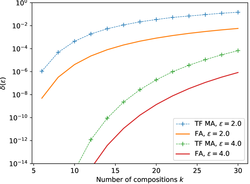
6.2 Heterogeneous Subsampled Gaussian Mechanism

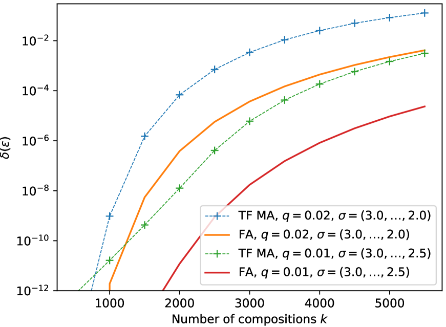
We next show how to compute $(\varepsilon,\delta)$-upper bounds for heterogeneous compositions of the subsampled Gaussian mechanism. We consider the Poisson subsampling and $\sim_{R}$-neighbouring relation. The fact that we obtain an upper bound in this case by considering non-adaptive compositions of univariate mechanisms is shown in the Appendix. For a subsampling ratio $q$ and noise level $\sigma$, the continuous PLD of the subsampled Gaussian mechanism is given by (Koskela et al.,, 2020)

$$\omega(s)=\begin{cases}f(g(s))g^{\prime}(s),&\text{ if }s>\log(1-q),\\ 0,&\text{ otherwise},\end{cases}$$

where

$$f(t)=\frac{1}{\sqrt{2\pi\sigma^{2}}}\,[q{\rm e}\hskip 1.0pt^{\frac{-(t-1)^{2}}{2\sigma^{2}}}+(1-q){\rm e}\hskip 1.0pt^{-\frac{t^{2}}{2\sigma^{2}}}],\quad g(s)=\sigma^{2}\log\left(\frac{{\rm e}\hskip 1.0pt^{s}-(1-q)}{q}\right)+\frac{1}{2}.$$

Analogously to (6.1), using $\omega$ we determine a discrete PLD $\omega_{\mathrm{max}}$, and by deriving a bound for the moment generating function of $\omega_{\mathrm{max}}$ (see also details in the Appendix) and by using Alg. 1 and Thm. 1 we obtain a numerical value $\delta_{\mathrm{max}}(\varepsilon)$ such that after $k$ compositions

$$\delta(\varepsilon)\leq\delta_{\mathrm{max}}(\varepsilon),$$

where $\delta(\varepsilon)$ gives a tight bound for the $k$-fold composition of heterogeneous subsampled Gaussian mechanisms. Figure 1(b) illustrates $\delta_{\mathrm{max}}(\varepsilon)$ as $k$ grows, when $L=10$ and $n=10^{6}$. For comparison, we also show the numerical values given by Tensorflow moments accountant (Abadi et al.,, 2016).

7 Conclusions

We have extended the Fast Fourier Transform-based approach for computing tight privacy bounds for discrete-valued mechanisms to heterogeneous compositions. We have given a complete error analysis of the method such that using the derived bounds it is possible to determine appropriate values for all the parameters of the algorithm, allowing more black-box like usage. The error analysis also led to a complexity bound that is slightly better than the existing theoretical complexity bound for non-adaptive compositions. Using the Plancherel theorem, we have shown how to further speed up the evaluation of DP bounds. We emphasise that due to the construction of the algorithm and to the rigorous error analysis, the reported $(\varepsilon,\delta)$-bounds are strict upper privacy bounds. One clear deficit of our approach, when compared to approaches such as GDP and RDP, is the difficulty of its implementation. However, in situations where accurate $(\varepsilon,\delta)$-bounds for compositions of complex mechanisms are required, the Fourier accountant appears as an attractive alternative.

Appendix A Comparisons to State-of-the-art DP Accountants

A.1 Comparison to the Rényi Differential Privacy accountant

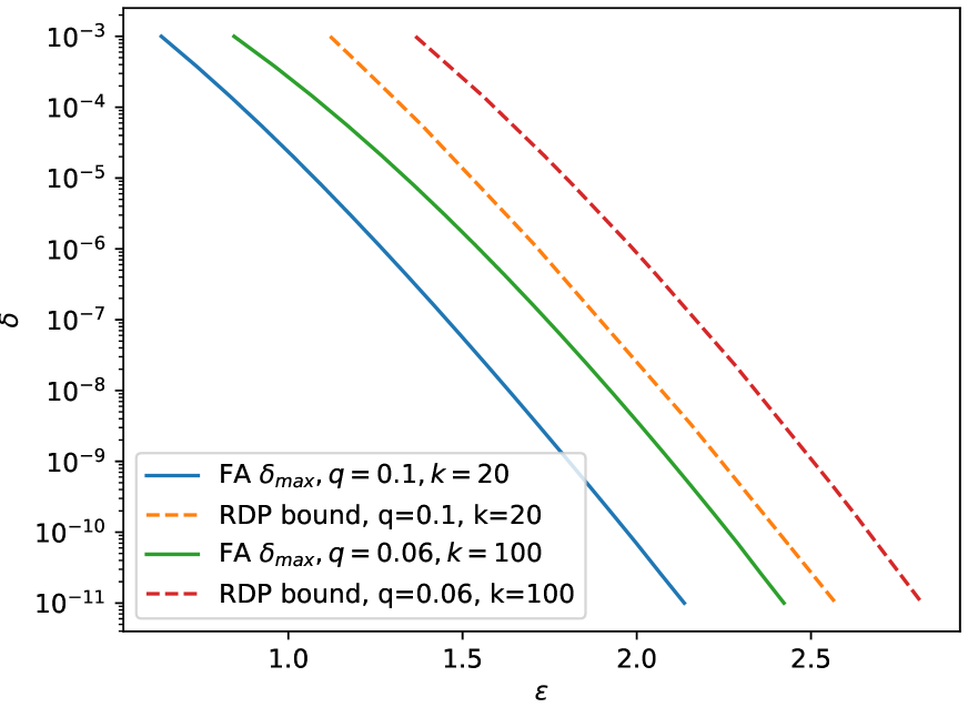
First, we compare our method to the RDP accountant by Zhu and Wang, (2019) which gives optimal RDP bounds for the subsampled Gaussian mechanism. This method is included in the ’autodp’ package  and it works for fixed values of $\sigma$ and $q$. Computing Fourier accountant (FA) bounds in the case where $\sigma$ drops linearly from 3.0 to 2.5 and the subsampling ratio $q$ is fixed, FA gives tighter bounds than the RDP accountant even for fixed $\sigma=3.0$ (see Fig. 2).

Figure 2: Upper $\varepsilon(\delta)$-bounds obtained using the Fourier Accountant and the Rényi DP accoutant ’autodp’. Here $\delta=10^{-6}$.

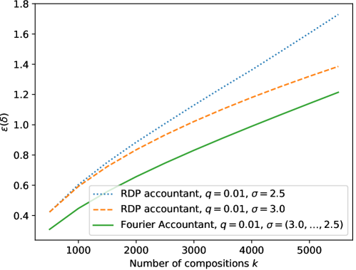
In Figures 2a and 2b we compare FA and ’autodp’ in case $\sigma$ is fixed for both. We fix $\sigma=2.0$ and vary the subsampling ratio $q$ and the number of compositions $k$. We see that FA gives considerably tighter bounds.

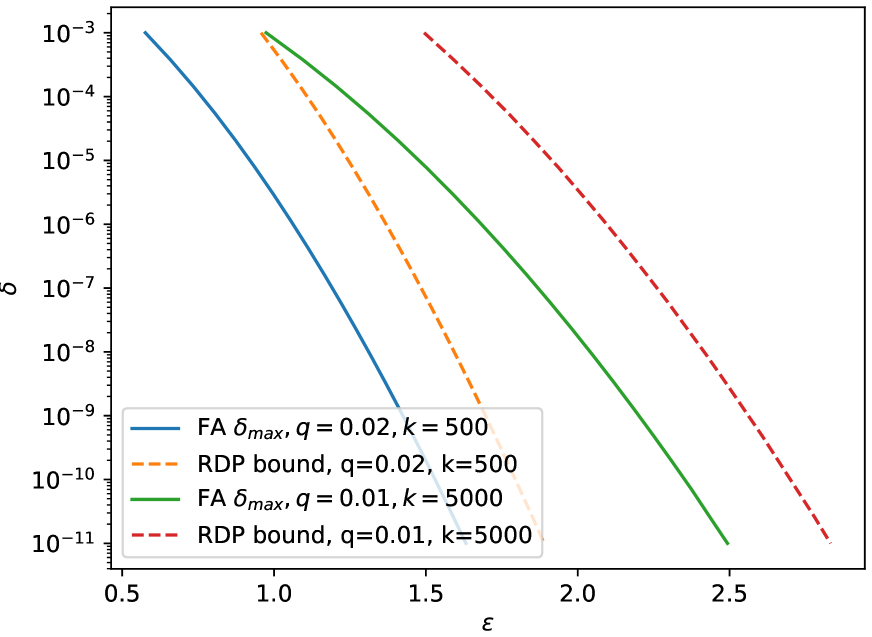
Part of the differences in these results is explained by the loss in converting RDP-values to $(\varepsilon,\delta)$-values. The conversion of the RDP-values to $(\varepsilon,\delta)$-values is carried out here using the formula (Zhu and Wang,, 2019) $\delta(\varepsilon)=\inf_{\alpha>1}{\rm e}\hskip 1.0pt^{-(\alpha-1)(\varepsilon-\gamma(\alpha)T)}.$ In the next subsection consider the possible gains of using a tighter conversion formula.

(a) $q=0.01$, $k=5000$ and $q=0.02$, $k=500$.

(b) $q=0.06$, $k=100$ and $q=0.1$, $k=20$.

Figure 3: Comparison of the upper and lower $\delta(\varepsilon)$-bounds given by FA and the RDP bound given by autodp, for various configurations when $\sigma=2.0$. Here $\varepsilon=1.0$.

A.2 Tighter Conversion of RDP to $(\varepsilon,\delta)$-DP

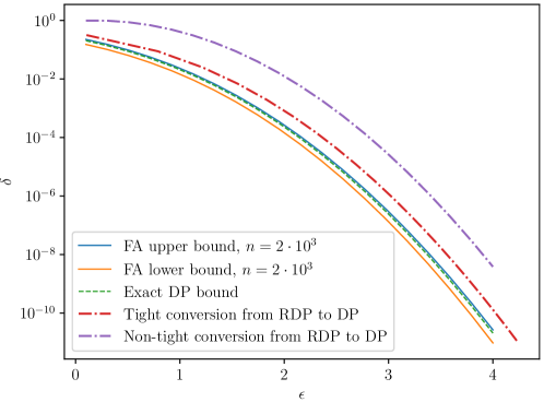
Asoodeh et al., (2020) consider a tighter conversion of RDP to $(\varepsilon,\delta)$-DP. The bound is optimal in a sense, that the obtained $(\varepsilon,\delta)$-values satisfy

$$\varepsilon_{\alpha}^{\delta}(\gamma)=\inf\{\varepsilon\geq 0\,:\,\forall\mathcal{M}\in\mathbb{M}_{\alpha}(\gamma)\textrm{ is }(\varepsilon,\delta)-\textrm{DP}\},$$

where $\mathbb{M}_{\alpha}(\gamma)$ denotes the set of all $(\alpha,\gamma)$-RDP mechanisms. As this definition suggests, the obtained $(\varepsilon,\delta)$-bounds are not necessarily tight DP-bounds for a given particular mechanism. Using log convex optimisation, Asoodeh et al., (2020) find $\varepsilon_{\alpha}^{\delta}(\gamma)$-upper bounds for the Gaussian mechanism from its RDP values (Asoodeh et al.,, 2020, Lemma 2). We illustrate the sub-optimality of the resulting $(\varepsilon,\delta)$-bounds as follows.

First of all, tight $(\varepsilon,\delta)$-bounds for the Gaussian mechanism are obtained as follows. For the PLD $\omega_{\mathrm{G}}$ of the Gaussian mechanism we know that (Sommer et al.,, 2019)

$$\omega_{\mathrm{G}}\leavevmode\nobreak\ \sim\mathcal{N}\left(\frac{1}{2\sigma^{2}},\frac{1}{\sigma^{2}}\right)$$

and for a $k$-wise composition, by convolution, we have that

$$\omega^{k}_{\mathrm{G}}\leavevmode\nobreak\ \sim\mathcal{N}\left(\frac{k}{2\sigma^{2}},\frac{k}{\sigma^{2}}\right).$$

The $(\varepsilon,\delta)$-values for this PLD are obtained by conversion involving the CDF of the Gaussian function (Sommer et al.,, 2019).

We know that the RDP-value of order $\alpha$ for the Gaussian mechanism is Mironov, (2017)

$$\gamma(\alpha)=\alpha/2\sigma^{2}.$$

We combine this RDP with the conversion formula of (Asoodeh et al.,, 2020, Lemma 2). We also compare the commonly used conversion formula (see e.g. Abadi et al.,, 2016, Thm. 2)

$$\delta(\varepsilon)=\inf_{\alpha>1}{\rm e}\hskip 1.0pt^{-(\alpha-1)(\varepsilon-\gamma(\alpha)T)}.$$ (A.1)

As Fig. 4 shows, the conversion by Asoodeh et al., (2020, Lemma 2) gives tighter results than the commonly used conversion formula (A.1), however the $\varepsilon_{\alpha}^{\delta}(\gamma)$-bound does not give tight $(\varepsilon,\delta)$-bounds whereas the bounds given by the Fourier accountant converge to the tight $(\varepsilon,\delta)$-bounds of the Gaussian mechanism.

Figure 4: Comparison of the Fourier Accountant and the RDP bounds obtained with different conversion methods. Here $k=6$ compositions. Here $n$ denotes the number of discretisation points for FA. We note that already for $n=10^{4}$ the upper and lower bounds given by FA become almost indistinguishable.

A.3 Comparison to the Gaussian Differential Privacy accountant

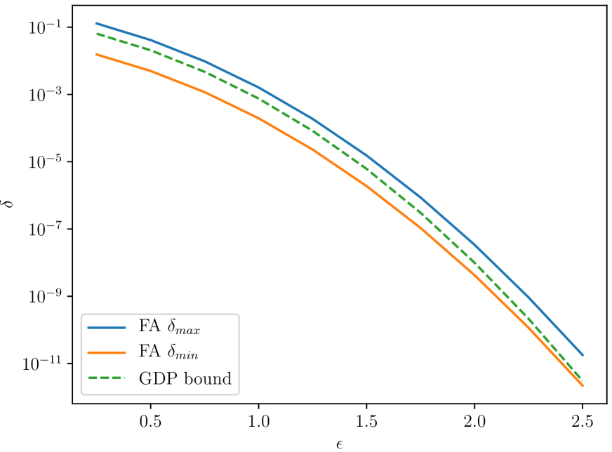
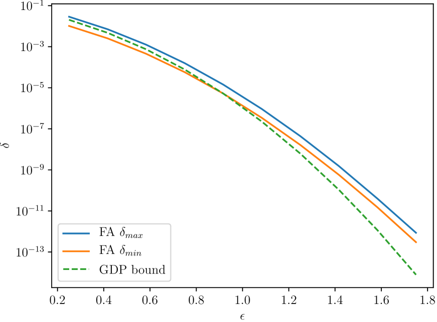
Gaussian Differential Privacy is an attractive alternative for privacy accounting as the bounds can be expressed using a single parameter $\mu$ (for more details, see Dong et al.,, 2021). Conversion to $(\varepsilon,\delta)$-bounds is straightforward using the CDF of the Gaussian function (Dong et al.,, 2021, Corollary 1). GDP gives exact $(\varepsilon,\delta)$-bounds for compositions of the Gaussian mechanism. For other mechanisms, for large numbers of compositions one can approximate the $\mu$-values using the central limit theorem. For example, in differentially private training of neural networks, the number of compositions is commonly several tens of thousands which makes the resulting GDP approximates accurate.

Dong et al., (2021, Section 4) provide also subsampling amplification results in case the subsample is of fixed size and uniformly sampled.  Bu et al., (2020) consider also the Poisson subsampling, and also an expression for the resulting DP bound is given, in terms of subsampling ratio $q$ and noise parameter $\sigma$ (see Sec. 3 Bu et al.,, 2020). Evaluating this expression analytically is difficult and therefore Bu et al., (2020) use the central limit theorem which says that after $k$ compositions the Poisson subsampled Gaussian mechanism is approximately $p\sqrt{k({\rm e}\hskip 1.0pt^{1/\sigma^{2}}-1)}$-GDP. This formula combined with the conversion formula (Corollary 1 Dong et al.,, 2021) is also the numerical method implemented in the Tensorflow libabry.

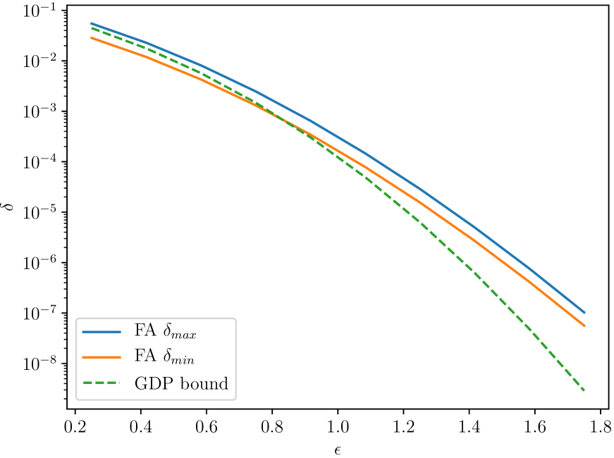
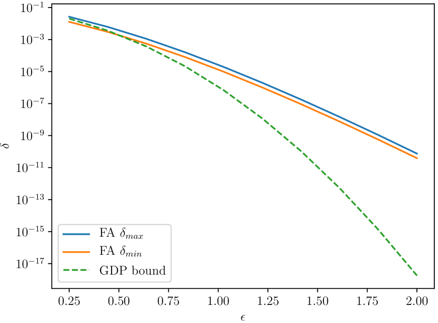
As these GDP results obtained using the Tensorflow accountant are approximations based on the central limit theorem (Bu et al.,, 2020) instead of strict upper bounds like the results of the Fourier Accountant, we expect them to give inaccurate results for small numbers of compositions $k$. This is indeed illustrated in Figure 5. We emphasise that the first figure ($k=5000$) is closest to a realistic scenario of a DP-SGD training.

(a) $n=10^{7}$, $q=0.01$, $k=5000$.

(b) $n=2\cdot 10^{6}$, $q=0.02$, $k=500$.

(c) $n=2\cdot 10^{5}$, $q=0.06$, $k=100$.

(d) $n=2\cdot 10^{4}$, $q=0.1$, $k=20$.

Figure 5: Comparison of the upper and lower $\delta(\varepsilon)$-bounds given by the Fourier Accountant and the approximative GDP bound, for different values of the subsampling ratio $q$ and different numbers of compositions $k$, when $\sigma=2.0$. For larger number of compositions, we use a larger number of discretisation points $n$ for the Fourier Accountant.

A.4 Few Conclusions About the Comparisons

Each of the DP accounting methods have their merits. Implementing GDP combined with a CLT approximation is extremely simple and for large numbers of homogeneous compositions (i.e. compositions where the mechanisms do not vary) the approximations based on the CLT give accurate results, as shown by the experiments of Figure 5. However, for small number of compositions, the Fourier accountant appears as superior compared to this approach.

The situation is similar when using RDP: implementing the accountant and understanding its functionality is often easier than that of the Fourier accountant. The improved conversion bounds proposed by Asoodeh et al., (2020) seem to give considerably tighter DP bounds than the commonly used conversion formula (Abadi et al.,, 2016). However, as illustrated by Figures 3 and 4, the difference in the $\delta$-upper bounds obtained using RDP and the Fourier accountant remains approximately at a one order of magnitude. Moreover, as also shown by the experiments of Koskela et al., (2020), for small number of compositions the Fourier accountant appears to give upper $\delta(\varepsilon)$-bounds that are several orders of magnitudes smaller. One clear benefit of the RDP approach is that it is more easily applicable to heterogeneous adaptive compositions, something that is more cumbersome when using the PLD approach.

The downside of the PLD approach is undoubtedly the complexity of the algorithm, there are simply much more lines of code involved and also possible pitfalls in the implementation. However in situations where accurate $(\varepsilon,\delta)$-bounds are required, and also for sanity-checking the functionality of other accountants by using simple non-adaptive compositions, the Fourier Accountant appears as an attractive alternative.

Appendix B Theorem 4 of the Main Text

Theorem 4 of the main text shows that the tight $(\varepsilon,\delta)$-bounds for compositions of non-adaptive mechanisms are obtained using convolutions of PLDs (see also Thm. 1 by Sommer et al., (2019)). We include the proof here for completeness.

Theorem 1.

Consider a non-adaptive composition of $k$ independent mechanisms $\mathcal{M}_{1},\ldots,\mathcal{M}_{k}$ and neighbouring data sets $X$ and $Y$. The composition is tightly $(\varepsilon,\delta)$-DP for $\delta(\varepsilon)$ given by

$$\delta(\varepsilon)=\max\{\delta_{X/Y}(\varepsilon),\delta_{Y/X}(\varepsilon)\},$$

where

$$\delta_{X/Y}(\varepsilon) =1-\prod\limits_{\ell=1}^{k}(1-\delta_{X/Y,\ell}(\infty))+\int_{\varepsilon}^{\infty}(1-{\rm e}\hskip 1.0pt^{\varepsilon-s})\left(\omega_{X/Y,1}*\cdots*\omega_{X/Y,k}\right)(s)\,\hskip 1.0pt{\rm d}\hskip 0.5pts,$$ (B.1)

$$\delta_{X/Y,\ell}(\infty) =\sum\limits_{\{t_{i}\,:\,\mathbb{P}(\mathcal{M_{\ell}}(X)=t_{i})>0,\,\mathbb{P}(\mathcal{M_{\ell}}(Y)=t_{i})=0\}}\mathbb{P}(\mathcal{M_{\ell}}(X)=t_{i})$$

and $\omega_{X/Y,1}*\cdots*\omega_{X/Y,k}$ denotes the convolution of the density functions $\omega_{X/Y,\ell}$, $1\leq\ell\leq k$. An analogous expression holds for $\delta_{Y/X}(\varepsilon)$.

Proof.

We show the proof first for the composition of two mechanisms. It will be clear from the proof how to generalise for a non-adaptive composition of $k$ mechanisms. We start by considering Lemma 4 of (Koskela et al.,, 2021) that gives an expression for the tight $(\varepsilon,\delta)$-DP bound for a single mechanism. By definition of the privacy loss distribution, the PLD distribution $\widetilde{\omega}$ of the non-adaptive composition of mechanisms $\mathcal{M}_{1}$ and $\mathcal{M}_{2}$ is given by

$$\widetilde{\omega}_{X/Y}(s) =\sum\limits_{(t_{i},t_{i}^{\prime})=(t_{j},t_{j}^{\prime})}\mathbb{P}\big{(}(\mathcal{M}_{1}(X),\mathcal{M}_{2}(X)=(t_{i},t_{i}^{\prime})\big{)}\cdot\delta_{\widetilde{s}_{i}}(s),$$

$$\quad\quad\widetilde{s}_{i}=\log\left(\frac{(\mathcal{M}_{1}(X),\mathcal{M}_{2}(X))=(t_{i},t_{i}^{\prime})}{(\mathcal{M}_{1}(Y),\mathcal{M}_{2}(Y)=(t_{j},t_{j}^{\prime})}\right).$$

Due to the independence of $\mathcal{M}_{1}$ and $\mathcal{M}_{2}$,

$$\mathbb{P}\big{(}\mathcal{M}_{1}(X) =t_{i},\,\mathcal{M}_{2}(X)=t_{i}^{\prime}\big{)}=\mathbb{P}\big{(}\mathcal{M}_{1}(X)=t_{i}\big{)}\,\mathbb{P}\big{(}\mathcal{M}_{2}(X)=t_{i}^{\prime}\big{)},$$ (B.2)

$$\mathbb{P}\big{(}\mathcal{M}_{1}(Y) =t_{j},\,\mathcal{M}_{2}(Y)=t_{j}^{\prime}\big{)}=\mathbb{P}\big{(}\mathcal{M}_{1}(Y)=t_{j}\big{)}\,\mathbb{P}\big{(}\mathcal{M}_{2}(Y)=t_{j}^{\prime}\big{)}.$$

Therefore,

$$\log\left(\frac{\mathbb{P}\big{(}\mathcal{M}_{1}(X)=t_{i},\,\mathcal{M}_{2}(X)=t_{i}^{\prime}\big{)}}{\mathbb{P}\big{(}\mathcal{M}_{1}(Y)=t_{j},\,\mathcal{M}_{2}(Y)=t_{j}^{\prime}\big{)}}\right)=\log\left(\frac{\mathbb{P}\big{(}\mathcal{M}_{1}(X)=t_{i}\big{)}}{\mathbb{P}\big{(}\mathcal{M}_{1}(Y)=t_{j}\big{)}}\right)+\log\left(\frac{\mathbb{P}\big{(}\mathcal{M}_{2}(X)=t_{i}^{\prime}\big{)}}{\mathbb{P}\big{(}\mathcal{M}_{2}(Y)=t_{j}^{\prime}\big{)}}\right).$$

and

$$\widetilde{\omega}_{X/Y}(s)=\sum\limits_{(t_{i},t_{i}^{\prime})=(t_{j},t_{j}^{\prime})}\mathbb{P}\big{(}\mathcal{M}_{1}(X)=t_{i}\big{)}\,\mathbb{P}\big{(}\mathcal{M}_{2}(X)=t_{i}^{\prime}\big{)}\cdot\delta_{s_{i}+s_{i}^{\prime}}(s),$$ (B.3)

where

$$s_{i}=\log\left(\frac{\mathbb{P}\big{(}\mathcal{M}_{1}(X)=t_{i}\big{)}}{\mathbb{P}\big{(}\mathcal{M}_{1}(Y)=t_{j}\big{)}}\right),\quad s_{i}^{\prime}=\log\left(\frac{\mathbb{P}\big{(}\mathcal{M}_{2}(X)=t_{i}^{\prime}\big{)}}{\mathbb{P}\big{(}\mathcal{M}_{2}(Y)=t_{j}^{\prime}\big{)}}\right).$$

We see from (B.3) that $\widetilde{\omega}_{X/Y}=\omega_{X/Y}*\omega_{X^{\prime}/Y^{\prime}}$ with discrete convolution $*$ as defined in the main text. The expression for $\widetilde{\delta}_{X/Y}(\infty)$ follows directly from its definition in Lemma 4 of (Koskela et al.,, 2021) that gives an expression for the tight $(\varepsilon,\delta)$-DP bound for a single mechanism, and from the independence of the mechanisms (B.2). We see from this proof and from the definition of the discrete convolution that the result directly generalises for a non-adaptive composition of $k$ mechanisms. ∎

Appendix C Proofs for the Results of Section 4

C.1 Lemma 5 of the Main Text

We first prove Lemma 5 of the main text. To that end, recall the grid approximation: we place PLDs on a grid

$$X_{n}=\{x_{0},\ldots,x_{n-1}\},\quad n\in\mathbb{Z}^{+},$$ (C.1)

where

$$x_{i}=-L+i\Delta x,\quad\Delta x=2L/n.$$

Suppose the PLD distribution $\omega$ is of the form

$$\omega(s)=\sum\nolimits_{i=0}^{n-1}a_{i}\cdot\delta_{s_{i}}(s),$$ (C.2)

where $a_{i}\geq 0$ and $-L\leq s_{i}\leq L-\Delta x$, $0\leq i\leq n-1$. We define the grid approximations

$$\omega^{\mathrm{L}}(s) :=\sum\nolimits_{i=0}^{n-1}a_{i}\cdot\delta_{s_{i}^{\mathrm{L}}}(s),$$ (C.3)

$$\omega^{\mathrm{R}}(s) :=\sum\nolimits_{i=0}^{n-1}a_{i}\cdot\delta_{s_{i}^{\mathrm{R}}}(s),$$

where

$$s_{i}^{\mathrm{L}} =\max\{x\in X_{n}\,:\,x\leq s_{i}\},$$

$$s_{i}^{\mathrm{R}} =\min\{x\in X_{n}\,:\,x\geq s_{i}\}.$$

Lemma 1.

Let $\delta(\varepsilon)$ be given by the integral formula of Theorem 4 of the main text for PLDs $\omega_{1},\cdots,\omega_{k}$ of the form (C.2). Let $\delta^{\mathrm{L}}(\varepsilon)$ and $\delta^{\mathrm{R}}(\varepsilon)$ correspondingly be determined by the left and right approximations $\omega_{1}^{\mathrm{L}},\ldots,\omega_{k}^{\mathrm{L}}$ and $\omega_{1}^{\mathrm{R}},\ldots,\omega_{k}^{\mathrm{R}}$, as defined in (C.3). Then for all $\varepsilon>0$ :

$$\delta^{\mathrm{L}}(\varepsilon)\leq\delta(\varepsilon)\leq\delta^{\mathrm{R}}(\varepsilon).$$ (C.4)

Proof.

Recall the integral formula of Theorem 4 of the main text:

$$\delta(\varepsilon)=1-\prod\limits_{\ell=1}^{k}(1-\delta_{\ell}(\infty))+\int_{\varepsilon}^{\infty}(1-{\rm e}\hskip 1.0pt^{\varepsilon-s})\left(\omega_{1}*\cdots*\omega_{k}\right)(s)\,\hskip 1.0pt{\rm d}\hskip 0.5pts.$$

As the probabilities $\delta_{\ell}(\infty)$ are not affected by the grid approximation, we may only consider bounds for the integral

$$\int_{\varepsilon}^{\infty}(1-{\rm e}\hskip 1.0pt^{\varepsilon-s})\left(\omega_{1}*\cdots*\omega_{k}\right)(s)\,\hskip 1.0pt{\rm d}\hskip 0.5pts.$$

By definition of the discrete convolution,

$$(\omega_{1}*\cdots*\omega_{k})(s)=\sum\nolimits_{i_{1},\ldots,i_{k}=0}^{n-1}a_{i_{1}}^{j}\cdots a_{i_{k}}^{j}\cdot\delta_{s_{i_{1}}+\ldots+s_{i_{k}}}(s)$$ (C.5)

and

$$(\omega_{1}^{\mathrm{L}}*\cdots*\omega_{k}^{\mathrm{L}})(s)=\sum\nolimits_{i_{1},\ldots,i_{k}=0}^{n-1}a_{i_{1}}^{j}\cdots a_{i_{k}}^{j}\cdot\delta_{s_{i_{1}}^{\mathrm{L}}+\ldots+s_{i_{k}}^{\mathrm{L}}}(s).$$ (C.6)

Since $(1-{\rm e}\hskip 1.0pt^{\varepsilon-s})$ is a monotonously increasing function of $s$ for $s\geq\varepsilon$, and since $s_{i_{1}}+\ldots+s_{i_{k}}\geq s_{i_{1}}^{\mathrm{L}}+\ldots+s_{i_{k}}^{\mathrm{L}}$ for all $(i_{1},\ldots,i_{k})$, we instantly see from (C.5) and (C.6) that

$$\delta^{\mathrm{L}}(\varepsilon)\leq\delta(\varepsilon).$$

For the right grid approximation, $s_{i_{1}}+\ldots+s_{i_{k}}\leq s_{i_{1}}^{\mathrm{R}}+\ldots+s_{i_{k}}^{\mathrm{R}}$ for all $(i_{1},\ldots,i_{k})$, and we similarly see that

$$\delta^{\mathrm{R}}(\varepsilon)\geq\delta(\varepsilon).$$

∎

C.2 Lemma 6 of the Main Text

We next prove Lemma 6 of the main text which shows that the truncated convolutions of periodic distributions can be evaluated using FFT. Suppose $\omega_{1}$ and $\omega_{2}$ are defined such that

$$\omega_{1}(s)=\sum\nolimits_{i}a_{i}\cdot\delta_{s_{i}}(s),\quad\omega_{2}(s)=\sum\nolimits_{i}b_{i}\cdot\delta_{s_{i}}(s),$$ (C.7)

where for all $i$: $a_{i},b_{i}\geq 0$ and $s_{i}=i\Delta x$. The convolution $\omega_{1}*\omega_{2}$ can then be written as

$$(\omega_{1}*\omega_{2})(s) =\sum\nolimits_{i,j}a_{i}b_{j}\cdot\delta_{s_{i}+s_{j}}(s)$$

$$=\sum\nolimits_{i}\Big{(}\sum\nolimits_{j}a_{j}b_{i-j}\Big{)}\cdot\delta_{s_{i}}(s).$$

Let $L>0$. We truncate these convolutions to the interval $[-L,L]$ such that

$$(\omega_{1}*\omega_{2})(s) \approx\sum\nolimits_{i}\Big{(}\sum\nolimits_{-L\leq s_{j}<L}a_{j}b_{i-j}\Big{)}\cdot\delta_{s_{i}}(s)$$

$$=:(\omega_{1}\circledast\omega_{2})(s).$$

For $\omega_{1}$ of the form (C.7), we define $\widetilde{\omega}_{1}$ to be a $2L$-periodic extension of $\omega_{1}$ from $[-L,L]$ to $\mathbb{R}$, i.e., $\widetilde{\omega}_{1}$ is of the form

$$\widetilde{\omega}_{1}(s)=\sum\nolimits_{m\in\mathbb{Z}}\,\sum\nolimits_{i}a_{i}\cdot\delta_{s_{i}+m\cdot 2L}(s).$$

For $\omega_{1}$ and $\omega_{2}$ of the form (C.7), we approximate the convolution $\omega_{1}*\omega_{2}$ as

$$\omega_{1}*\omega_{2}\approx\widetilde{\omega}_{1}\circledast\widetilde{\omega}_{2}.$$

Since $\omega_{1}$ and $\omega_{2}$ are defined on an equidistant grid, FFT can be used to evaluate the approximation $\widetilde{\omega}_{1}\circledast\widetilde{\omega}_{2}$ as follows:

Lemma 2 (Lemma 6 of the main text).

Let $\omega_{1}$ and $\omega_{2}$ be of the form (C.7), such that $s_{i}=-L+i\Delta x$, $0\leq i\leq n-1$, where $L>0$, $n$ is even and $\Delta x=2L/n$. Define

$$\boldsymbol{a} =\begin{bmatrix}a_{0}&\ldots&a_{n-1}\end{bmatrix}^{\mathrm{T}},$$

$$\quad\boldsymbol{b} =\begin{bmatrix}b_{0}&\ldots&b_{n-1}\end{bmatrix}^{\mathrm{T}},$$

$$D =\begin{bmatrix}0&I_{n/2}\\ I_{n/2}&0\end{bmatrix}\in\mathbb{R}^{n\times n}.$$

Then,

$$(\widetilde{\omega}_{1}\circledast\widetilde{\omega}_{2})(s)=\sum\nolimits_{i=0}^{n-1}c_{i}\cdot\delta_{s_{i}}(s),$$

where

$$c_{i}=\left[D\,\mathcal{F}^{-1}\big{(}\mathcal{F}(D\,\boldsymbol{a})\odot\mathcal{F}(D\,\boldsymbol{b})\big{)}\right]_{i},$$

and $\odot$ denotes the element-wise product of vectors.

Proof.

Assume $n$ is even and $s_{i}=-L+i\Delta x$, $0\leq i\leq n-1$. From the the truncation and periodisation it follows that $\widetilde{\omega}\circledast\widetilde{\omega}$ is of the form

$$(\widetilde{\omega}_{1}\circledast\widetilde{\omega}_{2})(s)=\sum\limits_{i=0}^{n-1}c_{i}\cdot\delta_{s_{i}}(s),\quad\quad c_{i}=\sum\limits_{j=n/2}^{3n/2-1}a_{j}\,b_{i-j}\,\textrm{ (indices modulo $n$)}.$$ (C.8)

Denoting $\boldsymbol{\widetilde{a}}=D\boldsymbol{a}$ and $\boldsymbol{\widetilde{b}}=D\boldsymbol{b}$, we see that the coefficients $c_{i}$ in (C.8) are given by the expression

$$c_{i+n/2}=\sum\limits_{j=0}^{n-1}\widetilde{a}_{j}\,\widetilde{b}_{i-j}\,\textrm{ (indices modulo $n$)},$$

to which we can apply DFT and the convolution theorem (Stockham Jr,, 1966). Thus, when $0\leq i\leq n-1$,

$$c_{i+n/2}=\left[\mathcal{F}^{-1}\big{(}\mathcal{F}(\boldsymbol{\widetilde{a}})\odot\mathcal{F}(\boldsymbol{\widetilde{b}})\big{)}\right]_{i}=\left[\mathcal{F}^{-1}\big{(}\mathcal{F}(D\boldsymbol{a})\odot\mathcal{F}(D\boldsymbol{b})\big{)}\right]_{i},\,\textrm{ (indices modulo $n$)}$$ (C.9)

where $\odot$ denotes the elementwise product of vectors. From (C.9) we find that

$$c_{i}=\left[D\mathcal{F}^{-1}\big{(}\mathcal{F}(D\boldsymbol{a})\odot\mathcal{F}(D\boldsymbol{b})\big{)}\right]_{i},\,\textrm{ (indices modulo $n$)}.$$

∎

Appendix D Proofs for the Results of Section 5

D.1 Decomposition of the Total Error

When carrying out the approximations described in the main text, we

1. First replace the PLDs $\omega_{1},\ldots,\omega_{k}$ by the right grid approximations $\omega_{1}^{\mathrm{R}},\ldots,\omega_{k}^{\mathrm{R}}$. Using the notation given in the main text, this corresponds to the approximation $\delta(\varepsilon)\approx\delta^{\mathrm{R}}(\varepsilon)$, i.e. to the approximation

   $$\int\limits_{L}^{\infty}(1-{\rm e}\hskip 1.0pt^{\varepsilon-s})(\omega_{1}*\cdots*\omega_{k})(s)\,\hskip 1.0pt{\rm d}\hskip 0.5pts\approx\int\limits_{L}^{\infty}(1-{\rm e}\hskip 1.0pt^{\varepsilon-s})(\omega_{1}^{\mathrm{R}}*\cdots*\omega_{k}^{\mathrm{R}})(s)\,\hskip 1.0pt{\rm d}\hskip 0.5pts.$$

2. Then, the Fourier accountant is used to approximate $\delta^{\mathrm{R}}(\varepsilon)\approx\widetilde{\delta^{\mathrm{R}}}(\varepsilon)$ which in exact arithmetic corresponds to the approximation

   $$\int\limits_{L}^{\infty}(1-{\rm e}\hskip 1.0pt^{\varepsilon-s})(\omega_{1}^{\mathrm{R}}*\cdots*\omega_{k}^{\mathrm{R}})(s)\,\hskip 1.0pt{\rm d}\hskip 0.5pts\approx\int\limits_{L}^{\infty}(1-{\rm e}\hskip 1.0pt^{\varepsilon-s})(\widetilde{\omega}_{1}^{\mathrm{R}}\circledast\cdots\circledast\widetilde{\omega}_{k}^{\mathrm{R}})(s)\,\hskip 1.0pt{\rm d}\hskip 0.5pts,$$

   where $\widetilde{\omega}_{i}$’s denote the periodised PLD distributions and $\circledast$ denotes the truncated convolutions (described in the main text).

We separately consider the errors arising from the periodisation and truncation of the convolutions and from the grid approximation. This means that we bound the total error as

$$\left|\delta(\varepsilon)-\widetilde{\delta^{\mathrm{R}}}(\varepsilon)\right| =\left|\delta(\varepsilon)-\delta^{\mathrm{R}}(\varepsilon)+\delta^{\mathrm{R}}(\varepsilon)-\widetilde{\delta^{\mathrm{R}}}(\varepsilon)\right|$$

$$\leq\left|\delta(\varepsilon)-\delta^{\mathrm{R}}(\varepsilon)\right|+\left|\delta^{\mathrm{R}}(\varepsilon)-\widetilde{\delta^{\mathrm{R}}}(\varepsilon)\right|$$

Theorem 8 of the main text gives a bound for the term $\left|\delta(\varepsilon)-\delta^{\mathrm{R}}(\varepsilon)\right|$ and Theorem 7 bounds for the term $\left|\delta(\varepsilon)-\widetilde{\delta}(\varepsilon)\right|$, in terms of the moment generating functions (MGFs) of $\omega_{1},\ldots,\omega_{k}$ and $-\omega_{1},\ldots,-\omega_{k}$. The bounds for the error $\left|\delta(\varepsilon)-\widetilde{\delta}(\varepsilon)\right|$ can be directly used to bound the error $\left|\delta^{\mathrm{R}}(\varepsilon)-\widetilde{\delta^{\mathrm{R}}}(\varepsilon)\right|$, either by numerically evaluating the MGFs of the PLDs $\omega_{1}^{\mathrm{R}},\ldots,\omega_{k}^{\mathrm{R}}$, or by using MGFs of the PLDs $\omega_{1},\ldots,\omega_{k}$ and Lemma 7 of Koskela et al., (2021), which states that when $0<\lambda<(\Delta x)^{-1}$,

$$\mathbb{E}[{\rm e}\hskip 1.0pt^{-\lambda\omega^{\mathrm{R}}}]\leq\mathbb{E}[{\rm e}\hskip 1.0pt^{-\lambda\omega}]\quad\textrm{and}\quad\mathbb{E}[{\rm e}\hskip 1.0pt^{\lambda\omega^{\mathrm{R}}}]\leq\tfrac{1}{1-\lambda\Delta x}\mathbb{E}[{\rm e}\hskip 1.0pt^{\lambda\omega}],$$

where $\Delta x=2L/n$.

D.2 Tail Bound for the Convolved PLDs

For the error analysis we repeatedly use the Chernoff bound (Wainwright,, 2019)

$$\mathbb{P}[X\geq t]=\mathbb{P}[{\rm e}\hskip 1.0pt^{\lambda X}\geq{\rm e}\hskip 1.0pt^{\lambda t}]\leq\frac{\mathbb{E}[{\rm e}\hskip 1.0pt^{\lambda X}]}{{\rm e}\hskip 1.0pt^{\lambda t}}$$

which holds for any random variable $X$ and for all $\lambda>0$. If $\omega$ is of the form

$$\omega(s)=\sum_{i=0}^{n-1}a_{i}\cdot\delta_{s_{i}}(s),\quad s_{i}=\log\left(\frac{a_{X,i}}{a_{Y,i}}\right),$$

where $a_{X,i},a_{Y,i}\geq 0$, $s_{i}\in\mathbb{R}$, $0\leq i\leq n-1$, the moment generating function is given by

$$\mathbb{E}[{\rm e}\hskip 1.0pt^{\lambda\omega_{X/Y}}] =\int\limits_{-\infty}^{\infty}{\rm e}\hskip 1.0pt^{\lambda s}\omega(s)\,\hskip 1.0pt{\rm d}\hskip 0.5pts=\sum\limits_{i=1}^{n}{\rm e}\hskip 1.0pt^{\lambda s_{i}}\cdot a_{X,i}=\sum\limits_{i=1}^{n}\left(\frac{a_{X,i}}{a_{Y,i}}\right)^{\lambda}a_{X,i}.$$ (D.1)

Denote $S_{k}:=\sum_{i=1}^{k}\omega_{i}$, where $\omega_{i}$ denotes the PLD random variable of the $i$th mechanism. Since $\omega_{i}$’s are independent, we have that

$$\mathbb{E}[{\rm e}\hskip 1.0pt^{\lambda S_{k}}]=\prod\nolimits_{i=1}^{k}\mathbb{E}[{\rm e}\hskip 1.0pt^{\lambda\omega_{i}}].$$

Then, the Chernoff bound shows that for any $\lambda>0$

$$I_{1}(L) =\int_{L}^{\infty}(\omega_{1}*\cdots*\omega_{k})(s)\,\hskip 1.0pt{\rm d}\hskip 0.5pts$$ (D.2)

$$=\mathbb{P}[S_{k}\geq L]$$

$$\leq\prod\nolimits_{i=1}^{k}\mathbb{E}[{\rm e}\hskip 1.0pt^{\lambda\omega_{i}}]\,{\rm e}\hskip 1.0pt^{-\lambda L}$$

$$\leq{\rm e}\hskip 1.0pt^{\sum_{i=1}^{k}\alpha_{i}(\lambda)}{\rm e}\hskip 1.0pt^{-\lambda L},$$

where $\alpha_{i}(\lambda)=\log(\mathbb{E}[{\rm e}\hskip 1.0pt^{\lambda\omega_{i}}])$.

D.3 Theorem 7 of the Main Text

We next give a proof for Theorem 7 of the main text. Recall: denote the logarithms of the moment generating functions of the PLDs as

$$\alpha_{i}^{+}(\lambda)=\log\Big{(}\mathbb{E}[{\rm e}\hskip 1.0pt^{\lambda\omega_{i}}]\Big{)},\quad\alpha_{i}^{-}(\lambda)=\log\Big{(}\mathbb{E}[{\rm e}\hskip 1.0pt^{-\lambda\omega_{i}}]\Big{)},$$

where $1\leq i\leq k$. Futhermore, denote

$$\alpha^{+}(\lambda)=\sum\nolimits_{i}\,\alpha^{+}_{i}(\lambda),\quad\alpha^{-}(\lambda)=\sum\nolimits_{i}\,\alpha^{-}_{i}(\lambda).$$

Using the Chernoff bound, we obtain the required using $\alpha^{+}(\lambda)$ and $\alpha^{-}(\lambda)$.

Remark 1.

Notice that in case $s_{j}\in[-L,L]$ for all $j$, $0\leq j\leq n-1$, then

$$(\omega_{1}\circledast\cdots\circledast\omega_{k})(s)=(\omega_{1}*\cdots*\omega_{k})(s),$$

i.e., the error arising from the truncation of discrete convolutions vanishes and Thm. 7 of the main text gives the total error arising from periodisation and truncation operations when $s_{j}\in[-L,L]$ for all $j$.

Theorem 2 (Thm. 7 of the main text).

Let $\omega$ be defined as above and suppose $s_{i}\in[-L,L]$ for all $0\leq i\leq n-1$. Then,

$$I_{3}(L)=\int\limits_{\varepsilon}^{L}\left|(\omega_{1}\circledast\cdots\circledast\omega_{k}-\widetilde{\omega}_{1}\circledast\cdots\circledast\widetilde{\omega}_{k})(s)\right|\,\hskip 1.0pt{\rm d}\hskip 0.5pts\leq\big{(}{\rm e}\hskip 1.0pt^{\alpha^{+}(\lambda)}+{\rm e}\hskip 1.0pt^{\alpha^{-}(\lambda)}\big{)}\frac{{\rm e}\hskip 1.0pt^{-L\lambda}}{1-{\rm e}\hskip 1.0pt^{-2L\lambda}}.$$

Proof.

Let $\omega_{i}$’s and the corresponding $2L$-periodic continuations $\widetilde{\omega}_{i}(s)$ be of the form

$$\omega_{i}(s)=\sum_{i}a_{j}^{i}\cdot\delta_{s_{j}}(s)\quad\textrm{and}\quad\widetilde{\omega}_{i}(s)=\sum_{j}\widetilde{a}_{j}^{i}\cdot\delta_{s_{j}}(s),$$

where $s_{j}=j\Delta x$ and $a_{j}^{i},\widetilde{a}_{j}^{i}\geq 0$. By definition of the truncated convolution $\circledast$,

$$(\widetilde{\omega}_{1}\circledast\cdots\circledast\widetilde{\omega}_{k})(s) =\sum\limits_{-L\leq s_{j_{1}}<L}\widetilde{a}_{j_{1}}^{1}\sum\limits_{-L\leq s_{j_{2}}<L}\widetilde{a}_{j_{2}}^{2}\ldots\sum\limits_{-L\leq s_{j_{k-1}}<L}\widetilde{a}_{j_{k-1}}^{k-1}\sum\limits_{i}\widetilde{a}_{i-j_{1}-\ldots-j_{k-1}}^{k}\cdot\delta_{s_{i}}(s)$$

$$=\sum\limits_{-L\leq s_{j_{1}}<L}a_{j_{1}}^{1}\sum\limits_{-L\leq s_{j_{2}}<L}a_{j_{2}}^{2}\ldots\sum\limits_{-L\leq s_{j_{k-1}}<L}a_{j_{k-1}}^{k-1}\sum\limits_{i}\widetilde{a}_{i-j_{1}-\ldots-j_{k-1}}^{k}\cdot\delta_{s_{i}}(s)$$

$$=\sum\limits_{j_{1}}a_{j_{1}}^{1}\sum\limits_{j_{2}}a_{j_{2}}^{2}\ldots\sum\limits_{j_{k-1}}a_{j_{k-1}}^{k-1}\sum\limits_{i}\widetilde{a}_{i-j_{1}-\ldots-j_{k-1}}^{k}\cdot\delta_{s_{i}}(s),$$

since for all $i$, $\widetilde{a}^{i}_{j}=a^{i}_{j}$ for all $j$ such that $-L\leq s_{j}<L$. Furthermore,

$$(\omega_{1}\circledast\cdots\circledast\omega_{k})(s) =\sum\limits_{-L\leq s_{j_{1}}<L}a_{j_{1}}^{1}\sum\limits_{-L\leq s_{j_{2}}<L}a_{j_{2}}^{2}\ldots\sum\limits_{-L\leq s_{j_{k-1}}<L}a_{j_{k-1}}^{k-1}\sum\limits_{i}a_{i-j_{1}-\ldots-j_{k-1}}^{k}\cdot\delta_{s_{i}}(s)$$

$$=\sum\limits_{j_{1}}a_{j_{1}}^{1}\sum\limits_{j_{2}}a_{j_{2}}^{2}\ldots\sum\limits_{j_{k-1}}a_{j_{k-1}}^{k-1}\sum\limits_{i}a_{i-j_{1}-\ldots-j_{k-1}}^{k}\cdot\delta_{s_{i}}(s).$$

Thus

$$(\widetilde{\omega}_{1}\circledast\cdots\circledast\widetilde{\omega}_{k}-\omega_{1}\circledast\cdots\circledast\omega_{k})(s)$$ (D.3)

$$\quad\quad\quad\quad=\sum\limits_{j_{1}}a_{j_{1}}^{1}\sum\limits_{j_{2}}a_{j_{2}}^{2}\ldots\sum\limits_{j_{k-1}}a_{j_{k-1}}^{k-1}\sum\limits_{i}\widehat{a}_{i-j_{1}-\ldots-j_{k-1}}^{k}\cdot\delta_{s_{i}}(s),$$

where

$$\widehat{a}^{k}_{j}=\widetilde{a}^{k}_{j}-a^{k}_{j}=\begin{cases}0,&\text{ if }-L\leq s_{j}<L,\\ a^{k}_{j\,\textrm{mod}\,n},&\text{ else. }\end{cases}$$ (D.4)

From (D.3) we see that

$$\int\limits_{\varepsilon}^{L}\left|(\omega_{1}\circledast\cdots\circledast\omega_{k}-\widetilde{\omega}_{1}\circledast\cdots\circledast\widetilde{\omega}_{k})(s)\right|\,\hskip 1.0pt{\rm d}\hskip 0.5pts$$ (D.5)

$$\quad\quad\leq\int\limits_{\mathbb{R}}\left|(\omega_{1}\circledast\cdots\circledast\omega_{k}-\widetilde{\omega}_{1}\circledast\cdots\circledast\widetilde{\omega}_{k})(s)\right|\,\hskip 1.0pt{\rm d}\hskip 0.5pts$$

$$\quad\quad=\int\limits_{\mathbb{R}}\sum\limits_{j_{1}}a_{j_{1}}^{1}\sum\limits_{j_{2}}a_{j_{2}}^{2}\ldots\sum\limits_{j_{k-1}}a_{j_{k-1}}^{k-1}\sum\limits_{i}\widehat{a}_{i-j_{1}-\ldots-j_{k-1}}^{k}\cdot\delta_{s_{i}}(s)\,\hskip 1.0pt{\rm d}\hskip 0.5pts$$

$$\quad\quad=\sum\limits_{j_{1}}a_{j_{1}}\sum\limits_{j_{1}}a_{j_{1}}^{1}\sum\limits_{j_{2}}a_{j_{2}}^{2}\ldots\sum\limits_{j_{k-1}}a_{j_{k-1}}^{k-1}\sum\limits_{i}\widehat{a}_{i-j_{1}-\ldots-j_{k-1}}^{k}.$$

From the periodic form of the coefficients $\widehat{a}^{k}_{j}$ (D.4) we have that

$$\sum\limits_{j_{1}}a_{j_{1}}^{1}\sum\limits_{j_{2}}a_{j_{2}}^{2}\ldots\sum\limits_{j_{k-1}}a_{j_{k-1}}^{k-1}\sum\limits_{i}\widehat{a}_{i-j_{1}-\ldots-j_{k-1}}^{k}$$ (D.6)

$$\quad\quad=\sum\limits_{n\in\mathbb{Z}\setminus\{0\}}\mathbb{P}\big{(}(2n-1)L\leq\omega_{1}*\cdots*\omega_{k}<(2n+1)L\big{)}$$

$$\quad\quad=\sum\limits_{n\in\mathbb{Z}^{-}}\mathbb{P}\big{(}(2n-1)L\leq\omega_{1}*\cdots*\omega_{k}<(2n+1)L\big{)}$$

$$\quad\quad\quad\quad+\sum\limits_{n\in\mathbb{Z}^{+}}\mathbb{P}\big{(}(2n-1)L\leq\omega_{1}*\cdots*\omega_{k}<(2n+1)L\big{)}$$

$$\quad\quad\leq\sum\limits_{n\in\mathbb{Z}^{-}}\mathbb{P}\big{(}\omega_{1}*\cdots*\omega_{k}\leq(2n+1)L\big{)}+\sum\limits_{n\in\mathbb{Z}^{+}}\mathbb{P}\big{(}\omega_{1}*\cdots*\omega_{k}\geq(2n-1)L\big{)}.$$

We also see that

$$\sum\limits_{n\in\mathbb{Z}^{-}}\mathbb{P}\big{(}\omega_{1}*\cdots*\omega_{k}\leq(2n+1)L\big{)}=\sum\limits_{n\in\mathbb{Z}^{+}}\mathbb{P}\big{(}(-\omega_{1})*\cdots*(-\omega_{k})\geq(2n-1)L\big{)}.$$

Using the Chernoff bound (D.2), we have the tail bound

$$\mathbb{P}\big{(}\omega_{1}*\cdots*\omega_{k}\geq(2n-1)L\big{)} \leq{\rm e}\hskip 1.0pt^{\sum_{i=1}^{k}\alpha_{i}(\lambda)}{\rm e}\hskip 1.0pt^{-(2n-1)L\lambda}$$

$$={\rm e}\hskip 1.0pt^{\alpha^{+}(\lambda)}{\rm e}\hskip 1.0pt^{-(2n-1)L\lambda}$$

and similarly

$$\mathbb{P}\big{(}(-\omega_{1})*\cdots*(-\omega_{k})\geq(2n-1)L\big{)}\leq{\rm e}\hskip 1.0pt^{\alpha^{-}(\lambda)}{\rm e}\hskip 1.0pt^{-(2n-1)L\lambda}.$$

Using the bounds (D.5), (D.6) and the Chernoff bound (D.2), we find that for all $\lambda>0$

$$\int\limits_{\varepsilon}^{L}\left|(\omega_{1}*\cdots*\omega_{k}-\widetilde{\omega}_{1}\circledast\cdots\circledast\widetilde{\omega}_{k})(s)\right|\,\hskip 1.0pt{\rm d}\hskip 0.5pts \leq\sum\limits_{\ell=1}^{\infty}{\rm e}\hskip 1.0pt^{\alpha^{+}(\lambda)}{\rm e}\hskip 1.0pt^{-(2\ell-1)L\lambda}+{\rm e}\hskip 1.0pt^{\alpha^{-}(\lambda)}{\rm e}\hskip 1.0pt^{-(2\ell-1)L\lambda}$$

$$=\big{(}{\rm e}\hskip 1.0pt^{\alpha^{+}(\lambda)}+{\rm e}\hskip 1.0pt^{\alpha^{-}(\lambda)}\big{)}\frac{{\rm e}\hskip 1.0pt^{-L\lambda}}{1-{\rm e}\hskip 1.0pt^{-2L\lambda}}.$$

∎

D.4 Thm. 7 of the main text, support of PLD outside of $[-L,L]$

For completeness, we consider also the case, where the PLD distribution is not contained in the $[-L,L]$-interval. This mean that, in addition to the periodisation error, we give also a bound for the truncation error (which does not vanish in this case)

$$\int\limits_{\varepsilon}^{L}\left|(\omega_{1}*\cdots*\omega_{k}-\omega_{1}\circledast\cdots\circledast\omega_{k})(s)\right|\,\hskip 1.0pt{\rm d}\hskip 0.5pts$$

in terms of the moment generating function of $\omega$.

Theorem 3.

Let $\omega_{i}$’s, $\alpha_{i}^{+}(\lambda)$’s and $\alpha_{i}^{-}(\lambda)$’s be defined as above. For all $\lambda>0$, we have that

$$I_{2}(L) =\int\limits_{\varepsilon}^{L}(\omega_{1}*\cdots*\omega_{k}-\omega_{1}\circledast\cdots\circledast\omega_{k})(s)\,\hskip 1.0pt{\rm d}\hskip 0.5pts$$

$$\leq\bigg{(}\frac{{\rm e}\hskip 1.0pt^{k\max_{i}\alpha_{i}^{+}(\lambda)}-{\rm e}\hskip 1.0pt^{\max_{i}\alpha_{i}^{+}(\lambda)}}{{\rm e}\hskip 1.0pt^{\max_{i}\alpha_{i}^{+}(\lambda)}-1}+\frac{{\rm e}\hskip 1.0pt^{k\max_{i}\alpha_{i}^{-}(\lambda)}-{\rm e}\hskip 1.0pt^{\max_{i}\alpha_{i}^{-}(\lambda)}}{{\rm e}\hskip 1.0pt^{\max_{i}\alpha_{i}^{-}(\lambda)}-1}\bigg{)}\,{\rm e}\hskip 1.0pt^{-L\lambda}.$$

Proof.

By adding and subtracting $(\omega_{1}*\cdots*\omega_{k-1})\circledast\omega_{k}$ , we may write

$$\omega_{1}*\cdots*\omega_{k}-\omega_{1}\circledast\cdots\circledast\omega_{k}$$ (D.7)

$$= (\omega_{1}*\cdots*\omega_{k-1})*\omega_{k}-(\omega_{1}*\cdots*\omega_{k-1})\circledast\omega_{k}$$

$$\quad+(\omega_{1}*\cdots*\omega_{k-1}-\omega_{1}\circledast\cdots\circledast\omega_{k-1})\circledast\omega_{k}.$$

Let $\ell\in\mathbb{Z}^{+}$. Let $\omega_{\ell}$ be of the form

$$\omega_{\ell}(s)=\sum_{j}a_{j}^{\ell}\cdot\delta_{s_{j}}(s)$$

and let the convolution $\omega*\cdots*\omega_{\ell-1}$ be of the form

$$(\omega*\cdots*\omega_{\ell-1})(s)=\sum_{j}c_{j}\cdot\delta_{s_{j}}(s)$$

for some $a^{\ell}_{j},c_{j}\geq 0$, $s_{j}=j\Delta x$. From the definition of the operators $*$ and $\circledast$ it follows that

$$\big{(}(\omega*\cdots*\omega_{\ell-1})*\omega_{\ell}-(\omega*\cdots*\omega_{\ell-1})\circledast\omega_{\ell}\big{)}(s)$$

$$\quad\quad=\sum\limits_{j_{1}}\Big{(}\sum\limits_{j_{2}}c_{j_{2}}a_{j_{1}-j_{2}}\Big{)}\cdot\delta_{s_{j_{1}}}(s)-\sum\limits_{j_{1}}\Big{(}\sum\limits_{-L\leq s_{j_{2}}<L}c_{j_{2}}a_{j_{1}-j_{2}}\Big{)}\cdot\delta_{s_{j_{1}}}(s)$$

$$\quad\quad=\sum\limits_{j_{1}}\Big{(}\sum\limits_{s_{j_{2}}<-L,\,s_{j_{2}}\geq L}c_{j_{2}}a_{j_{1}-j_{2}}\Big{)}\cdot\delta_{s_{j_{1}}}(s).$$

Therefore,

$$\int\limits_{\mathbb{R}}\big{(}(\omega*\cdots*\omega_{\ell-1})*\omega_{\ell}-(\omega*\cdots*\omega_{\ell-1})\circledast\omega_{\ell}\big{)}(s)\,\hskip 1.0pt{\rm d}\hskip 0.5pts$$ (D.8)

$$\quad\quad=\int\limits_{\mathbb{R}}\sum\limits_{j_{1}}\Big{(}\sum\limits_{s_{j_{2}}<-L,\,s_{j_{2}}\geq L}c_{j_{2}}a_{j_{1}-j_{2}}^{\ell}\Big{)}\cdot\delta_{s_{j_{1}}}(s)\,\hskip 1.0pt{\rm d}\hskip 0.5pts$$

$$\quad\quad=\sum\limits_{s_{j_{2}}<-L,\,s_{j_{2}}\geq L}c_{j_{2}}\sum\limits_{j_{1}}\int\limits_{\mathbb{R}}a_{j_{1}-j_{2}}^{\ell}\cdot\delta_{s_{j_{1}}}(s)\,\hskip 1.0pt{\rm d}\hskip 0.5pts$$

$$\quad\quad=\sum\limits_{s_{j_{2}}<-L,\,s_{j_{2}}\geq L}c_{j_{2}}\sum\limits_{j_{1}}a_{j_{1}-j_{2}}^{\ell}$$

$$\quad\quad=\sum\limits_{s_{j_{2}}<-L,\,s_{j_{2}}\geq L}c_{j_{2}}$$

$$\quad\quad=\,\mathbb{P}\Big{(}\omega_{1}*\cdots*\omega_{\ell-1}<-L\Big{)}+\mathbb{P}\Big{(}\omega_{1}*\cdots*\omega_{\ell-1}\geq L\Big{)}$$

$$\quad\quad\leq\,{\rm e}\hskip 1.0pt^{\sum\nolimits_{i=1}^{\ell-1}\alpha_{i}^{+}(\lambda)}{\rm e}\hskip 1.0pt^{-L\lambda}+{\rm e}\hskip 1.0pt^{\sum\nolimits_{i=1}^{\ell-1}\alpha_{i}^{-}(\lambda)}{\rm e}\hskip 1.0pt^{-L\lambda}$$

$$\quad\quad\leq\,{\rm e}\hskip 1.0pt^{(\ell-1)\max_{i}\alpha_{i}^{+}(\lambda)}{\rm e}\hskip 1.0pt^{-L\lambda}+{\rm e}\hskip 1.0pt^{(\ell-1)\max_{i}\alpha_{i}^{-}(\lambda)}{\rm e}\hskip 1.0pt^{-L\lambda}$$

for all $\lambda>0$. The second last inequality follows from the Chernoff bound.

Similarly, suppose $\omega_{1}*\cdots*\omega_{\ell-1}-\omega_{1}\circledast\cdots\circledast\omega_{\ell-1}$ is of the form

$$(\omega_{1}*\cdots*\omega_{\ell-1}-\omega_{1}\circledast\cdots\circledast\omega_{\ell-1})(s)=\sum_{i}\widetilde{c}_{i}\cdot\delta_{s_{i}}(s)$$

for some coefficients $\widetilde{c}_{i}\geq 0$, where $s_{i}=i\Delta x$. Then,

$$\int\limits_{\mathbb{R}}\big{(}(\omega_{1}*\cdots*\omega_{\ell-1}-\omega_{1}\circledast\cdots\circledast\omega_{\ell-1})\circledast\omega_{\ell}\big{)}(s)\,\hskip 1.0pt{\rm d}\hskip 0.5pts$$ (D.9)

$$\quad\quad=\int\limits_{\mathbb{R}}\sum\limits_{j_{1}}\Big{(}\sum\limits_{-L\leq s_{j_{2}}<L}\widetilde{c}_{j}a_{{j_{1}}-{j_{2}}}^{\ell}\Big{)}\cdot\delta_{s_{j_{1}}}(s)\,\hskip 1.0pt{\rm d}\hskip 0.5pts$$

$$\quad\quad=\sum\limits_{-L\leq s_{j_{2}}<L}\widetilde{c}_{j_{2}}\int\limits_{\mathbb{R}}\sum\limits_{i}a_{{j_{1}}-{j_{2}}}^{\ell}\cdot\delta_{s_{j_{1}}}(s)\,\hskip 1.0pt{\rm d}\hskip 0.5pts$$

$$\quad\quad=\sum\limits_{-L\leq s_{j_{2}}<L}\widetilde{c}_{j_{2}}$$

$$\quad\quad\leq\int\limits_{\mathbb{R}}(\omega_{1}*\cdots*\omega_{\ell-1}-\omega_{1}\circledast\cdots\circledast\omega_{\ell-1})(s)\,\hskip 1.0pt{\rm d}\hskip 0.5pts.$$

Using (D.7), (D.8) and (D.9), we see that for all $\lambda>0$,

$$\int\limits_{\varepsilon}^{L}(\omega_{1}*\cdots*\omega_{k}-\omega_{1}\circledast\cdots\circledast\omega_{k})(s)\,\hskip 1.0pt{\rm d}\hskip 0.5pts$$ (D.10)

$$\quad\quad\leq\int\limits_{\mathbb{R}}(\omega_{1}*\cdots*\omega_{k}-\omega_{1}\circledast\cdots\circledast\omega_{k})(s)\,\hskip 1.0pt{\rm d}\hskip 0.5pts$$

$$\quad\quad\leq{\rm e}\hskip 1.0pt^{(k-1)\max_{i}\alpha_{i}^{+}(\lambda)}{\rm e}\hskip 1.0pt^{-L\lambda}+{\rm e}\hskip 1.0pt^{(k-1)\max_{i}\alpha_{i}^{-}(\lambda)}{\rm e}\hskip 1.0pt^{-L\lambda}$$

$$\quad\quad\quad\quad+\int\limits_{\mathbb{R}}(\omega_{1}*\cdots*\omega_{k-1}-\omega_{1}\circledast\cdots\circledast\omega_{k-1}\omega)(s)\,\hskip 1.0pt{\rm d}\hskip 0.5pts.$$

Using (D.10) recursively, we see that for all $\lambda>0$, we have

$$\int\limits_{\varepsilon}^{L}(\omega_{1}*\cdots*\omega_{k}-\omega_{1}\circledast\cdots\circledast\omega_{k})(s)\,\hskip 1.0pt{\rm d}\hskip 0.5pts$$

$$\quad\quad\leq\sum\limits_{\ell=1}^{k-1}{\rm e}\hskip 1.0pt^{\ell\max_{i}\alpha_{i}^{+}(\lambda)}{\rm e}\hskip 1.0pt^{-L\lambda}+\sum\limits_{\ell=1}^{k-1}{\rm e}\hskip 1.0pt^{\ell\max_{i}\alpha_{i}^{-}(\lambda)}{\rm e}\hskip 1.0pt^{-L\lambda}$$

$$\quad\quad=\bigg{(}\frac{{\rm e}\hskip 1.0pt^{k\max_{i}\alpha_{i}^{+}(\lambda)}-{\rm e}\hskip 1.0pt^{\max_{i}\alpha_{i}^{+}(\lambda)}}{{\rm e}\hskip 1.0pt^{\max_{i}\alpha_{i}^{+}(\lambda)}-1}+\frac{{\rm e}\hskip 1.0pt^{k\max_{i}\alpha_{i}^{-}(\lambda)}-{\rm e}\hskip 1.0pt^{\max_{i}\alpha_{i}^{-}(\lambda)}}{{\rm e}\hskip 1.0pt^{\max_{i}\alpha_{i}^{-}(\lambda)}-1}\bigg{)}\,{\rm e}\hskip 1.0pt^{-L\lambda}.$$

∎

D.5 Theorem 8 of the main text

We next give a proof for Theorem 8 of the main text which gives a bound for the grid approximation error.

Theorem 4 (Thm. 8 of the main text).

The discretisation error $\delta^{\mathrm{R}}(\varepsilon)-\delta(\varepsilon)$ can be bounded as

$$\delta^{\mathrm{R}}(\varepsilon)-\delta(\varepsilon)\leq k\Delta x\,\big{(}\mathbb{P}(\omega_{1}+\cdots+\omega_{k}\geq\varepsilon)-\delta(\varepsilon)\big{)}.$$

Proof.

From the definition of the discrete convolution we see that

$$(\omega_{1}*\cdots*\omega_{k})(s)=\sum\limits_{i_{1},\ldots,i_{k}}a^{1}_{i_{1}}\cdots\,a^{k}_{i_{k}}\cdot\delta_{s^{1}_{i_{1}}+\ldots+s^{k}_{i_{k}}}(s)$$

and that

$$\delta(\varepsilon) =\int\nolimits_{\varepsilon}^{\infty}(1-{\rm e}\hskip 1.0pt^{\varepsilon-s})\,(\omega_{1}*\cdots*\omega_{k})(s)\,\hskip 1.0pt{\rm d}\hskip 0.5pts$$

$$=\sum\limits_{\{i_{1},\ldots,i_{k}\,:\,s^{1}_{i_{1}}+\ldots+s^{k}_{i_{k}}\geq\varepsilon\}}a^{1}_{i_{1}}\cdots\,a^{k}_{i_{k}}\cdot(1-{\rm e}\hskip 1.0pt^{\varepsilon-s^{1}_{i_{1}}-\ldots-s^{k}_{i_{k}}})$$

Then, using the inequality

$$a\leq b\Rightarrow\exp(b)-\exp(a)\leq\exp(b)(b-a),$$

we have that

$$\delta^{\mathrm{R}}(\varepsilon)-\delta(\varepsilon)= \sum\limits_{\{i_{1},\ldots,i_{k}\,:\,s^{1}_{i_{1}}+\ldots+s^{k}_{i_{k}}\geq\varepsilon\}}a^{1}_{i_{1}}\cdots\,a^{k}_{i_{k}}\cdot({\rm e}\hskip 1.0pt^{\varepsilon-s^{1}_{i_{1}}-\ldots-s^{k}_{i_{k}}}-{\rm e}\hskip 1.0pt^{\varepsilon-s_{i_{1}}^{\mathrm{R},1}-\ldots-s_{i_{k}}^{\mathrm{R},k}})$$

$$\leq \sum\limits_{\{i_{1},\ldots,i_{k}\,:\,s^{1}_{i_{1}}+\ldots+s^{k}_{i_{k}}\geq\varepsilon\}}a^{1}_{i_{1}}\cdots\,a^{k}_{i_{k}}\cdot\big{(}(s_{i_{1}}^{\mathrm{R},1}-s^{1}_{i_{1}})+\ldots+(s_{i_{k}}^{\mathrm{R},k}-s^{k}_{i_{k}})\big{)}\cdot{\rm e}\hskip 1.0pt^{\varepsilon-s^{1}_{i_{1}}-\ldots-s^{k}_{i_{k}}}.$$

Since $s_{i}^{\mathrm{R},\ell}-s^{\ell}_{i}\leq\Delta x$ for all $i$ and $\ell$, we have that

$$\delta^{\mathrm{R}}(\varepsilon)-\delta(\varepsilon) \leq\,k\Delta x\sum\limits_{\{i_{1},\ldots,i_{k}\,:\,s^{1}_{i_{1}}+\ldots+s^{k}_{i_{k}}\geq\varepsilon\}}a^{1}_{i_{1}}\cdots\,a^{k}_{i_{k}}\cdot{\rm e}\hskip 1.0pt^{\varepsilon-s^{1}_{i_{1}}-\ldots-s^{k}_{i_{k}}}$$

$$=\,k\Delta x\big{(}\sum\limits_{\{i_{1},\ldots,i_{k}\,:\,s^{1}_{i_{1}}+\ldots+s^{k}_{i_{k}}\geq\varepsilon\}}a^{1}_{i_{1}}\cdots\,a^{k}_{i_{k}}$$

$$-\sum\limits_{\{i_{1},\ldots,i_{k}\,:\,s^{1}_{i_{1}}+\ldots+s^{k}_{i_{k}}\geq\varepsilon\}}a^{1}_{i_{1}}\cdots\,a^{k}_{i_{k}}\cdot(1-{\rm e}\hskip 1.0pt^{\varepsilon-s^{1}_{i_{1}}-\ldots-s^{k}_{i_{k}}})\big{)}$$

$$=k\Delta x\,\big{(}\mathbb{P}(\omega_{1}*\cdots*\omega_{k}\geq\varepsilon)-\delta(\varepsilon)\big{)}.$$

∎

D.6 Lemma 10 the Main Text: Upper Bound for the Computational Complexity

We next prove the computational complexity result of Lemma 10 of the main text. For simplicity, we assume in the following that the compositions consist of $(\varepsilon,0)$-DP mechanisms and that the parameter $L$ is chose sufficiently large so that for all $i$: $\left|s_{i}\right|\leq L$, where $s_{i}=\log\tfrac{a_{X,i}}{a_{Y,i}}$. Then, we can bound the periodisation error using Theorem 7 of the main text.

Recall: we denote the logarithms of the moment generating functions of the PLDs as

$$\alpha_{i}^{+}(\lambda)=\log\Big{(}\mathbb{E}[{\rm e}\hskip 1.0pt^{\lambda\omega_{i}}]\Big{)},\quad\alpha_{i}^{-}(\lambda)=\log\Big{(}\mathbb{E}[{\rm e}\hskip 1.0pt^{-\lambda\omega_{i}}]\Big{)},$$ (D.11)

where $1\leq i\leq k$. Futhermore, denote

$$\alpha^{+}(\lambda)=\sum\nolimits_{i}\,\alpha^{+}_{i}(\lambda),\quad\alpha^{-}(\lambda)=\sum\nolimits_{i}\,\alpha^{-}_{i}(\lambda).$$

Lemma 5.

Consider a non-adaptive composition of the mechanisms $\mathcal{M}_{1},\ldots,\mathcal{M}_{k}$ with corresponding worst-case pairs of distributions $f_{X,i}$ and $f_{Y,i}$, $1\leq i\leq k$. Suppose the sequence $\mathcal{M}_{1},\ldots,\mathcal{M}_{k}$ consists of $m$ distinct mechanisms. Then, it is possible to have an approximation of $\delta(\varepsilon)$ with error less than $\eta$ with number of operations

$$\mathcal{O}\left(\frac{mk^{2}C_{k}}{\eta}\log\frac{k^{2}C_{k}}{\eta}\right),$$

where

$$C_{k}=\max\{\tfrac{1}{k}\sum_{i}D_{\infty}(f_{X,i}||f_{Y,i}),\tfrac{1}{k}\sum_{i}D_{\infty}(f_{Y,i}||f_{X,i})\}$$

and

$$D_{\infty}(f_{X}||f_{Y})=\sup_{a_{Y,i}\neq 0}\log\frac{a_{X,i}}{a_{Y,i}}.$$

Proof.

We first determine a lower bound for the truncation parameter $L$ in terms of $k$. Consider the right-hand-side of the error bound of Theorem 7 of the main text. Suppose $L\geq 1$ and $\lambda\geq 1$. Then, we have that

$$\big{(}{\rm e}\hskip 1.0pt^{\alpha^{+}(\lambda)}+{\rm e}\hskip 1.0pt^{\alpha^{-}(\lambda)}\big{)}\,\frac{{\rm e}\hskip 1.0pt^{-L\lambda}}{1-{\rm e}\hskip 1.0pt^{-2L\lambda}} \leq\big{(}{\rm e}\hskip 1.0pt^{\alpha^{+}(\lambda)}+{\rm e}\hskip 1.0pt^{\alpha^{-}(\lambda)}\big{)}\cdot\frac{{\rm e}\hskip 1.0pt}{2}\cdot{\rm e}\hskip 1.0pt^{-L\lambda},$$ (D.12)

$$\leq{\rm e}\hskip 1.0pt^{\max\{{\alpha^{-}(\lambda),\alpha^{+}(\lambda)}\}+1}{\rm e}\hskip 1.0pt^{-L\lambda},$$

where $\alpha^{-}(\lambda)$ and $\alpha^{+}(\lambda)$ are defined as above in (D.11).

For each $i$, the logarithm of the moment-generating function of the PLD can be expressed in terms of the Rényi divergence Mironov, (2017):

$$\log\Big{(}\mathbb{E}[{\rm e}\hskip 1.0pt^{\lambda\omega_{X/Y,i}}]\Big{)} =\lambda\cdot\frac{1}{\lambda}\sum_{i}\left(\frac{a_{X,i}}{a_{Y,i}}\right)^{\lambda}a_{X,i}$$

$$=\lambda\cdot\frac{1}{\lambda}\sum_{i}\left(\frac{a_{X,i}}{a_{Y,i}}\right)^{\lambda+1}a_{Y,i}$$

$$=\lambda\cdot D_{\lambda+1}(f_{X}||f_{Y}),$$

where $D_{\lambda}$ denotes the Rényi divergence of order $\lambda$. From the monotonicity of Rényi divergence (see Proposition 9, Mironov, (2017)) it follows that

$$\alpha^{+}(\lambda) =\lambda\cdot\sum\nolimits_{i}D_{\lambda+1}(f_{X,i}||f_{Y,i})$$

$$\leq\lambda\cdot\sum\nolimits_{i}D_{\infty}(f_{X,i}||f_{Y,i}),$$

where

$$D_{\infty}(f_{X}||f_{Y})=\sup_{a_{Y,i}\neq 0}\log\frac{a_{X,i}}{a_{Y,i}}.$$

With a similar calculation, we find that

$$\alpha^{-}(\lambda)\leq(\lambda-1)\cdot\sum\nolimits_{i}D_{\infty}(f_{Y,i}||f_{X,i}).$$

Thus,

$$\max\{{\alpha^{-}(\lambda),\alpha^{+}(\lambda)}\}\leq k\lambda\cdot\max\{\tfrac{1}{k}\sum_{i}D_{\infty}(f_{X,i}||f_{Y,i}),\tfrac{1}{k}\sum_{i}D_{\infty}(f_{Y,i}||f_{X,i})\}.$$

Now we can further bound (D.12) from above as

$${\rm e}\hskip 1.0pt^{\max\{{\alpha^{-}(\lambda),\alpha^{+}(\lambda)}\}+1}{\rm e}\hskip 1.0pt^{-L\lambda}\leq{\rm e}\hskip 1.0pt^{k\lambda\cdot C_{k}+1}{\rm e}\hskip 1.0pt^{-L\lambda},$$

where

$$C_{k}=\max\{\tfrac{1}{k}\sum_{i}D_{\infty}(f_{X,i}||f_{Y,i}),\tfrac{1}{k}\sum_{i}D_{\infty}(f_{Y,i}||f_{X,i})\}.$$

Requiring this upper bound to be smaller than a prescribed $\eta>0$, and setting $\lambda=1$, we arrive at the condition

$$L\geq k\cdot C_{k}+1+\log\frac{1}{\eta}.$$ (D.13)

Next, we bound the computational complexity using a bound for the discretisation error. From Thm. 8 of the main text it follows that the discretisation error is bounded as

$$\delta^{\mathrm{R}}(\varepsilon)-\delta(\varepsilon)\leq k\Delta x=\frac{2Lk}{n}.$$

Requiring this discretisation error to be less than $\eta$, choosing $L$ according to (D.13) and assuming $k\geq\log\frac{1}{\eta}$, we see that choosing

$$n=\mathcal{O}\left(\frac{k^{2}C_{k}}{\eta}\right)$$

is sufficient for the sum of the error sources to be less than $2\eta$. As we need to compute FFT for $m$ different PLDs, and since FFT has complexity $n\log n$, we see that with

$$\mathcal{O}\left(\frac{2mk^{2}C_{k}}{\eta}\log\frac{k^{2}C_{k}}{\eta}\right)$$

operations it is possible to have an approximation of $\delta(\varepsilon)$ with error less than $\eta$, and that additional factor in the leading constant is given by the leading constant in the complexity of FFT.

∎

Remark 6.

We see from the proof, that for the condition that the periodisation error is less than $\eta$, it is sufficient to choose

$$L\geq\frac{\log\eta^{-1}+\max\{{\alpha^{-}(\lambda),\alpha^{+}(\lambda)}\}+1}{\lambda}.$$

As this is true for all $\lambda\geq 1$ and since $\alpha^{-}(\lambda)$ and $\alpha^{+}(\lambda)$ can be evaluated numerically, a sufficient value of $L$ can be found via an optimisation problem. Notice also that since $\alpha^{-}(\lambda)$ and $\alpha^{+}(\lambda)$ correspond to cumulant generating functions (CGFs) (Abadi et al.,, 2016), and since the minimisation problem

$$\min_{\lambda}\frac{\log\delta^{-1}+\alpha(\lambda)}{\lambda}$$

is exactly the conversion formula for turning CGF-values to $(\varepsilon(\delta),\delta)$-DP values, we see that approximately (assuming $\lambda^{-1}$ is small) $L$ has to be chosen as

$$L\geq\varepsilon(\eta),$$

where $\varepsilon(\eta)$ gives $(\varepsilon,\delta)$-DP of the composition $(\mathcal{M}_{1},\ldots,\mathcal{M}_{k})$ at $\delta=\eta$.

D.7 Fast Evaluation Using the Plancherel Theorem

We next prove Lemma 11 of the main text. Recall the Fourier accountant algorithm of the main text. When using this algorithm to approximate $\delta(\varepsilon)$, we need to evaluate the expression

$$\boldsymbol{b}^{k}=D\,\mathcal{F}^{-1}\big{(}\mathcal{F}(D\boldsymbol{a})^{\odot k}\big{)}$$ (D.14)

and the sum

$$\widetilde{\delta}(\varepsilon)=\sum\nolimits_{-L+\ell\Delta x>\varepsilon}\big{(}1-{\rm e}\hskip 1.0pt^{\varepsilon-(-L+\ell\Delta x)}\big{)}\,b^{k}_{\ell}.$$ (D.15)

The following lemma shows that when evaluating $\widetilde{\delta}(\varepsilon)$ for different numbers of compositions $k$, the updates of $\widetilde{\delta}(\varepsilon)$ can be performed in $\mathcal{O}(n)$ time.

Lemma 7.

Denote $\boldsymbol{w}_{\varepsilon}\in\mathbb{R}^{n}$ such that

$$(\boldsymbol{w}_{\varepsilon})_{\ell}=\max\{1-{\rm e}\hskip 1.0pt^{\varepsilon-(-L+\ell\Delta x)},0\}$$

and let $\boldsymbol{b}^{k}$ be of the form (D.14). Then, we have that

$$\widetilde{\delta}(\varepsilon)=\frac{1}{n}\langle\mathcal{F}(D\boldsymbol{w}_{\varepsilon}),\mathcal{F}(D\boldsymbol{a})^{\odot k}\rangle.$$ (D.16)

Proof.

We see that the sum (D.15) is given by the following inner product:

$$\widetilde{\delta}(\varepsilon)=\langle\boldsymbol{w}_{\varepsilon},\boldsymbol{b}^{k}\rangle.$$

The Plancherel Theorem states that the discrete Fourier transform preserves inner products: for $x,y\in\mathbb{R}^{n}$,

$$\langle x,y\rangle=\frac{1}{n}\langle\mathcal{F}x,\mathcal{F}y\rangle.$$ (D.17)

Using (D.17), we see that

$$\widetilde{\delta}(\varepsilon) =\langle\boldsymbol{w}_{\varepsilon},\boldsymbol{b}^{k}\rangle$$

$$=\langle\boldsymbol{w}_{\varepsilon},D\mathcal{F}^{-1}\big{(}\mathcal{F}(D\boldsymbol{a})^{\odot k}\big{)}\rangle$$

$$=\langle D\boldsymbol{w}_{\varepsilon},\mathcal{F}^{-1}\big{(}\mathcal{F}(D\boldsymbol{a})^{\odot k}\big{)}\rangle$$

$$=\frac{1}{n}\langle\mathcal{F}(D\boldsymbol{w}),\mathcal{F}(D\boldsymbol{a})^{\odot k}\rangle.$$

∎

Appendix E Details for the Experiments of Section 6

In order to use the Fourier accountant for compositions including continuous mechanisms, we first need to discretise the PLDs of the continuous mechanism appropriately. This means that we replace each continuous PLD $\omega$ by a certain discrete-valued distribution $\omega_{\mathrm{max}}$ that leads to an overall $\delta(\varepsilon)$-upper bound. This procedure is analogous to what is considered in the experiments of Koskela et al., (2021) for the homogeneous composition of subsampled Gaussian mechanisms (see the supplementary material of Koskela et al.,, 2021). Those results can be used to derive the discrete PLDs for the experiments of Sec. 6.2., i.e., for the heterogeneous composition of subsampled Gaussian mechanisms.

E.1 Experiments of Section 6.1

For the PLD $\omega_{\mathrm{G}}$ of the Gaussian mechanism we know that (Sommer et al.,, 2019)

$$\omega_{\mathrm{G}}\leavevmode\nobreak\ \sim\mathcal{N}\left(\frac{1}{2\sigma^{2}},\frac{1}{\sigma^{2}}\right).$$

Let $L>0$, $n\in\mathbb{Z}^{+}$, $\Delta x=2L/n$ and let the grid $X_{n}$ be defined as in Section 4.2 of the main text. Define

$$\omega_{\mathrm{max}}(s)=\sum\limits_{i=0}^{n-1}c^{+}_{i}\cdot\delta_{s_{i}}(s),$$

where $s_{i}=i\Delta x$ and

$$c^{+}_{i}=\Delta x\cdot\max\limits_{s\in[s_{i-1},s_{i}]}\omega_{\mathrm{G}}(s),$$ (E.1)

and define

$$\omega^{\infty}_{\mathrm{max}}(s)=\sum\limits_{i\in\mathbb{Z}}c^{+}_{i}\cdot\delta_{s_{i}}(s).$$ (E.2)

To obtain rigorous $\delta(\varepsilon)$-bounds for the compositions, we carry out the error analysis for the distribution $\omega^{\infty}_{\mathrm{max}}$ and use Theorem 3 above. To this end, we need bounds for the moment generating functions of $-\omega^{\infty}_{\mathrm{max}}$ and $\omega^{\infty}_{\mathrm{max}}$.

To show that $\omega^{\infty}_{\mathrm{max}}$ indeed leads to an upper bound for $\delta(\varepsilon)$, we refer to (supplementary material of Koskela et al.,, 2021), where this is shown for the compositions of the subsampled Gaussian mechanism. The proof here goes analogously, and we have that for all $\varepsilon>0$,

$$\delta(\varepsilon)\leq\delta_{\mathrm{max}}^{\infty}(\varepsilon),$$

where $\delta_{\mathrm{max}}^{\infty}(\varepsilon)$ is the tight bound for the composition involving $\omega^{\infty}_{\mathrm{max}}$.

To evaluate $\alpha^{+}(\lambda)$ and $\alpha^{-}(\lambda)$ for the upper bound of Theorem 3, we need the moment generating functions of $-\omega^{\infty}_{\mathrm{max}}$ and $\omega^{\infty}_{\mathrm{max}}$. We have the following bound for $\omega^{\infty}_{\mathrm{max}}$. We note that $\mathbb{E}[{\rm e}\hskip 1.0pt^{\lambda\omega_{\mathrm{max}}}]$ can be evaluated numerically.

Lemma 1.

Let $0<\lambda\leq L$ and assume $\sigma\geq 1$ and $\Delta x\leq c\cdot L$, $0<c<1$. The moment generating function of $\omega^{\infty}_{\mathrm{max}}$ can be bounded as

$$\mathbb{E}[{\rm e}\hskip 1.0pt^{\lambda\omega^{\infty}_{\mathrm{max}}}]\leq\mathbb{E}[{\rm e}\hskip 1.0pt^{\lambda\omega_{\mathrm{max}}}]+\mathrm{err}(\lambda,L,\sigma),$$

where

$$\mathrm{err}(\lambda,L,\sigma)=\exp\bigg{(}\frac{3\lambda}{2\sigma^{2}}\bigg{)}\left(\int_{-\infty}^{-L}\widetilde{\omega}(s)\,\hskip 1.0pt{\rm d}\hskip 0.5pts+\int_{L-\Delta x}^{\infty}\widetilde{\omega}(s)\,\hskip 1.0pt{\rm d}\hskip 0.5pts\right),\quad\widetilde{\omega}\leavevmode\nobreak\ \sim\mathcal{N}\left(\frac{1+2\lambda}{2\sigma^{2}},\frac{1}{\sigma^{2}}\right).$$ (E.3)

Proof.

The moment generating function of $\omega^{\infty}_{\mathrm{max}}$ is given by

$$\mathbb{E}[{\rm e}\hskip 1.0pt^{\lambda\omega^{\infty}_{\mathrm{max}}}] =\int_{-L}^{L}{\rm e}\hskip 1.0pt^{\lambda s}\omega^{\infty}_{\mathrm{max}}(s)\,\hskip 1.0pt{\rm d}\hskip 0.5pts+\int_{-\infty}^{-L}{\rm e}\hskip 1.0pt^{\lambda s}\omega^{\infty}_{\mathrm{max}}(s)\,\hskip 1.0pt{\rm d}\hskip 0.5pts+\int_{L}^{\infty}{\rm e}\hskip 1.0pt^{\lambda s}\omega^{\infty}_{\mathrm{max}}(s)\,\hskip 1.0pt{\rm d}\hskip 0.5pts$$ (E.4)

$$\leq\mathbb{E}[{\rm e}\hskip 1.0pt^{\lambda\omega_{\mathrm{max}}}]+\int_{-\infty}^{-L}{\rm e}\hskip 1.0pt^{\lambda s}\omega_{\mathrm{G}}(s)\,\hskip 1.0pt{\rm d}\hskip 0.5pts+\int_{L-\Delta x}^{\infty}{\rm e}\hskip 1.0pt^{\lambda s}\omega_{\mathrm{G}}(s)\,\hskip 1.0pt{\rm d}\hskip 0.5pts$$

We arrive at the claim by observing that for $\omega_{\mathrm{G}}\leavevmode\nobreak\ \sim\mathcal{N}\left(\frac{1}{2\sigma^{2}},\frac{1}{\sigma^{2}}\right)$,

$$\int_{-\infty}^{-L}{\rm e}\hskip 1.0pt^{\lambda s}\omega_{\mathrm{G}}(s)\,\hskip 1.0pt{\rm d}\hskip 0.5pts=\exp\bigg{(}\frac{3\lambda}{2\sigma^{2}}\bigg{)}\int_{-\infty}^{-L}\widetilde{\omega}(s)\,\hskip 1.0pt{\rm d}\hskip 0.5pts,$$

where $\widetilde{\omega}\leavevmode\nobreak\ \sim\mathcal{N}\left(\frac{1+2\lambda}{2\sigma^{2}},\frac{1}{\sigma^{2}}\right)$ and similarly for the second term in (E.3). ∎

Using a reasoning analogous to the proof of Lemma 1, we get the following. We note that $\mathbb{E}[{\rm e}\hskip 1.0pt^{-\lambda\omega_{\mathrm{min}}}]$ can be evaluated numerically.

Corollary 2.

The moment generating function of $-\omega^{\infty}_{\mathrm{max}}$ can be bounded as

$$\mathbb{E}[{\rm e}\hskip 1.0pt^{-\lambda\omega^{\infty}_{\mathrm{max}}}]\leq\mathbb{E}[{\rm e}\hskip 1.0pt^{-\lambda\omega_{\mathrm{max}}}]+\mathrm{err}(\lambda,L,\sigma),$$

where $\mathrm{err}(\lambda,L,\sigma)$ is defined as in (E.3).

Remark 3.

In the experiments, the error term $\mathrm{err}(\lambda,L,\sigma)$ was found to be negligible.

Appendix F Tight $(\varepsilon,\delta)$-Bound for an Adaptive Composition of Multivariate Subsampled Gaussian Mechanisms Using One-Dimensional Distributions

We next give a rigorous proof for the fact that the multivariate subsampled Gaussian mechanism with Poisson subsampling can be analysed by one-dimensional Gaussian mixtures. The proof is motivated by an analogous result (Mironov et al.,, 2019, Thm. 4) which is for RDP and we partly use the notation used in the proof of that result. For simplicity, we focus here on the case, where the underlying function is of the summative form

$$F(X,\theta)=\sum_{x\in X}g(x,\theta),$$ (F.1)

where $g$ is Lipschitz-continuous w.r.t. $\theta$ and has a 2-norm bounded by a constant $c>0$.

We show the equivalence part by part so that first in Section F.2 we show the equivalence for a single iteration of the mechanism and then in Section F.3 we show the equivalence rigorously for the multivariate Gaussian mechanism. Then, by combining these results arrive at the conclusion.

F.1 Motivational Example: DP-SGD

The motivational example to consider functions of the form (F.7) is DP-SGD, where the terms $g(\theta,x)$ are the sample-wise clipped gradients. When applying DP-SGD to, for example, neural networks, the gradients can be assumed to be Lipschitz continuous in bounded sets (a condition sufficient for our analysis). As the following result verifies, then are also the clipped gradients Lipschitz continuous.

Lemma 1.

Suppose the function $h(\theta)$, $h\,:\,S\rightarrow\mathbb{R}^{d}$ is $L$-Lipschitz continuous in $S\subset\mathbb{R}^{d}$. Then, also the function

$$g(\theta)=\mathrm{clip}_{c}\big{(}h\big{)}(\theta)=\frac{h(\theta)}{\max\{1,\frac{\|h(\theta)\|_{2}}{c}\}}$$

is $L$-Lipschitz in $S$.

Proof.

Let $x,y\in S$. If $\|h(x)\|_{2}\leq c$ or $\|h(y)\|_{2}\leq c$, or if $\langle h(x),h(y)\rangle<0$, the inequality

$$\|g(x)-g(y)\|_{2}\leq\|h(x)-h(y)\|_{2}.$$

follows by simple geometry. Assume $\|h(x)\|_{2}>c$, $\|h(y)\|_{2}>c$ and $\langle h(x),h(y)\rangle\geq 0$. Then,

$$\|g(x)-g(y)\|_{2}^{2} =\|g(x)\|_{2}^{2}+\|g(y)\|_{2}^{2}-2\langle g(x),g(y)\rangle$$

$$=2c^{2}\cdot\big{(}1-\langle\tfrac{h(x)}{\|h(x)\|_{2}},\tfrac{h(y)}{\|h(y)\|_{2}}\rangle\big{)}$$

$$\leq 2\|h(x)\|_{2}\|h(y)\|_{2}\cdot\big{(}1-\langle\tfrac{h(x)}{\|h(x)\|_{2}},\tfrac{h(y)}{\|h(y)\|_{2}}\rangle\big{)}$$

$$=2\|h(x)\|_{2}\|h(y)\|_{2}-2\langle h(x),h(y)\rangle$$

$$\leq\|h(x)\|_{2}^{2}+\|h(y)\|_{2}^{2}-2\langle h(x),h(y)\rangle$$

$$=\|h(x)-h(y)\|_{2}^{2}.$$

∎

F.2 The Subsampled Gaussian Mechanism with Poisson Subsampling

We first show the analogy for a single iteration of the mechanism, in a case where the underlying function $g$ is differentiable w.r.t. $\theta$ and has a norm exactly 1 for all data samples $x$ and for all $\theta$. We will use the following notation repeatedly in the proof.

Definition 2.

Let $\varepsilon>0$ and $\delta\in[0,1]$. Let $P$ and $Q$ be two random variables taking values in a measurable space $\mathcal{R}$. We say that $P$ and $Q$ are $(\varepsilon,\delta)$-indistinguishable, denoted $P\simeq_{(\varepsilon,\delta)}Q$, if for every measurable set $E\subset\mathcal{R}$ we have

$$\mathrm{Pr}(P\in E)\leq{\rm e}\hskip 1.0pt^{\varepsilon}\mathrm{Pr}(Q\in E)+\delta\quad\textrm{and}\quad\mathrm{Pr}(Q\in E)\leq{\rm e}\hskip 1.0pt^{\varepsilon}\mathrm{Pr}(P\in E)+\delta.$$

Theorem 3.

If

$$\mathcal{N}(0,\sigma^{2})\simeq_{(\varepsilon,\delta)}(1-q)\cdot\mathcal{N}\big{(}0,\sigma^{2}\big{)}+q\cdot\mathcal{N}\big{(}1,\sigma^{2}\big{)},$$

where $(1-q)\cdot\mathcal{N}(0,\sigma^{2})+q\cdot\mathcal{N}(1,\sigma^{2})$ denotes a mixture of $\mathcal{N}(0,\sigma^{2})$ and $\mathcal{N}(1,\sigma^{2})$, then also the multivariate Poisson subsampled Gaussian mechanism with subsampling ratio $q$ and variance $\sigma^{2}$ and $L_{2}$-sensitivity $1$ is $(\varepsilon,\delta)$-DP.

Proof.

Similarly to the proof of (Mironov et al.,, 2019, Thm. 4), let $T$ denote a set-valued random variable defined by taking a random subset of $X\in\mathcal{X}^{N}$, where each element of $X$ is independently placed in $T$ with probability $q$. For simplicity, suppose that $f(T)$ is of the summative form

$$f(T)=\sum_{x\in T}g(x),$$

where $\|g(x)\|_{2}=1$ for all $x\in X$. Conditioned on $T$, the mechanism $\mathcal{M}(X)$ samples from a Gaussian with mean $f(T)$. Then, $\mathcal{M}(X)$ can be represented as a mixture

$$\mathcal{M}(X)=\sum_{T}p_{T}\cdot\mathcal{N}(f(T),\sigma^{2}I_{d}),$$

where the sum denotes mixing of the distributions with the weights $p_{T}$.

Let $X^{\prime}\in\mathcal{X}^{N}$ be a neighbouring dataset such that $X^{\prime}=X\cup\{x^{\prime}\}$. Then, we have

$$\mathcal{M}(X^{\prime})=\sum_{T}p_{T}\cdot\bigg{(}(1-q)\cdot\mathcal{N}\big{(}f(T),\sigma^{2}I_{d}\big{)}+q\cdot\mathcal{N}\big{(}f(T)+g(x^{\prime}),\sigma^{2}I_{d}\big{)}\bigg{)}.$$

(Rotation) Consider an orthogonal matrix $U\in\mathbb{R}^{d\times d}$ of the form

$$U=\begin{bmatrix}g(x^{\prime})&\widetilde{U}\end{bmatrix},$$

where $\widetilde{U}\in\mathbb{R}^{d\times(d-1)}$. Again, $\widetilde{U}$ can be taken as any $d\times(d-1)$ matrix such that the columns of $U$ give an orthonormal basis of $\mathbb{R}^{d}$. Then, in particular, we have that

$$U^{\mathrm{T}}\Delta=e_{1},$$

where $e_{1}=\begin{bmatrix}1&0&\ldots&0\end{bmatrix}^{T}$. We see that the fact that $\mathcal{M}(X)\simeq_{(\varepsilon,\delta)}\mathcal{M}(X^{\prime})$ is equivalent to the fact that $U^{T}\mathcal{M}(X)\simeq_{(\varepsilon,\delta)}U^{T}\mathcal{M}(X^{\prime})$. Clearly,

$$U^{T}\mathcal{M}(X)\sim\sum_{T}p_{T}\cdot\mathcal{N}(U^{T}f(T),\sigma^{2}I_{d})$$

since $U$ is orthogonal. Similarly

$$U^{T}\mathcal{M}(X^{\prime})\sim\sum_{T}p_{T}\cdot\bigg{(}(1-q)\cdot\mathcal{N}\big{(}U^{T}f(T),\sigma^{2}I_{d}\big{)}+q\cdot\mathcal{N}\big{(}U^{T}(f(T)+g(x^{\prime})),\sigma^{2}I_{d}\big{)}\bigg{)}.$$

(Translation) Clearly for each subset $T$ of $X$,

$$\mathcal{N}(U^{T}f(T),\sigma^{2}I_{d})\simeq_{(\varepsilon,\delta)}(1-q)\cdot\mathcal{N}\big{(}U^{T}f(T),\sigma^{2}I_{d}\big{)}+q\cdot\mathcal{N}\big{(}U^{T}(f(T)+g(x^{\prime})),\sigma^{2}I_{d}\big{)}$$ (F.2)

if and only if

$$\mathcal{N}(0,\sigma^{2}I_{d})\simeq_{(\varepsilon,\delta)}(1-q)\cdot\mathcal{N}\big{(}0,\sigma^{2}I_{d}\big{)}+q\cdot\mathcal{N}\big{(}U^{T}g(x^{\prime}),\sigma^{2}I_{d}\big{)}.$$ (F.3)

Since $U^{T}g(x^{\prime})=e_{1}$, and the coordinate-wise noises in the mechanisms of (F.3) are independent, (F.3) holds if and only if

$$\mathcal{N}(0,\sigma^{2})\simeq_{(\varepsilon,\delta)}(1-q)\cdot\mathcal{N}\big{(}0,\sigma^{2}\big{)}+q\cdot\mathcal{N}\big{(}1,\sigma^{2}\big{)}.$$ (F.4)

Thus, (F.2) holds if and only if (F.4) holds.

Now suppose

$$\mathcal{N}(0,\sigma^{2})\simeq_{(\varepsilon,\delta)}(1-q)\cdot\mathcal{N}\big{(}0,\sigma^{2}\big{)}+q\cdot\mathcal{N}\big{(}1,\sigma^{2}\big{)}.$$

Let $S\subset\mathbb{R}^{d}$. Using the reasoning above, we have

$$\mathbb{P}(U^{T}\mathcal{M}(X^{\prime})\subset S) =\mathbb{P}(U^{T}\mathcal{M}(X^{\prime})\subset S)$$

$$=\mathbb{P}\bigg{(}\sum_{T}p_{T}\cdot\big{(}(1-q)\cdot\mathcal{N}\big{(}U^{T}f(T),\sigma^{2}I_{d}\big{)}+q\cdot\mathcal{N}\big{(}U^{T}(f(T)+g(x^{\prime})),\sigma^{2}I_{d}\big{)}\big{)}\subset S\bigg{)}$$

$$=\sum_{T}p_{T}\cdot\mathbb{P}\bigg{(}\big{(}(1-q)\cdot\mathcal{N}\big{(}U^{T}f(T),\sigma^{2}I_{d}\big{)}+q\cdot\mathcal{N}\big{(}U^{T}(f(T)+g(x^{\prime})),\sigma^{2}I_{d}\big{)}\big{)}\subset S\bigg{)}$$

$$\leq\sum_{T}p_{T}\bigg{(}{\rm e}\hskip 1.0pt^{\varepsilon}\mathbb{P}(\mathcal{N}(U^{T}f(T),\sigma^{2}I_{d})\subset S)+\delta\bigg{)}$$

$$={\rm e}\hskip 1.0pt^{\varepsilon}\sum_{T}p_{T}\cdot\mathbb{P}\big{(}\mathcal{N}(U^{T}f(T),\sigma^{2}I_{d})\subset S\big{)}+\sum_{T}p_{T}\cdot\delta$$

$$={\rm e}\hskip 1.0pt^{\varepsilon}\mathbb{P}\big{(}\sum_{T}p_{T}\cdot\mathcal{N}(U^{T}f(T),\sigma^{2}I_{d})\subset S\big{)}+\delta$$

$$={\rm e}\hskip 1.0pt^{\varepsilon}\mathbb{P}\big{(}U^{T}\mathcal{M}(X)\subset S\big{)}+\delta.$$

Similarly, we see that

$${\rm e}\hskip 1.0pt^{\varepsilon}\mathbb{P}\big{(}U^{T}\mathcal{M}(X)\subset S\big{)}\leq\mathbb{P}(U^{T}\mathcal{M}(X^{\prime})\subset S)+\delta.$$

Since the fact that $\mathcal{M}(X)\simeq_{(\varepsilon,\delta)}\mathcal{M}(X^{\prime})$is equivalent to the fact that $U^{T}\mathcal{M}(X)\simeq_{(\varepsilon,\delta)}U^{T}\mathcal{M}(X^{\prime})$, we see that $\mathcal{M}(X)\simeq_{(\varepsilon,\delta)}\mathcal{M}(X^{\prime})$.

∎

F.3 Adaptive Compositions

The PLD approach is directly applicable to non-adaptive compositions of the form

$$\mathcal{M}(X)=\big{(}\mathcal{M}_{1}(X),\ldots,\mathcal{M}_{k}(X)\big{)}.$$ (F.5)

The adaptive compositions we consider are of the form

$$\mathcal{M}(X,\theta)=\big{(}\mathcal{M}_{1}(X,\theta),\mathcal{M}_{2}\big{(}X,\mathcal{M}_{1}(X,\theta)\big{)},\ldots,\mathcal{M}_{k}\big{(}X,\mathcal{M}_{k-1}(X,\ldots)\big{)}.$$

We want to bound the tight $(\varepsilon,\delta)$-values of the adaptive composition with the a non-adaptive composition of the form (F.5). We first recall an integral representation for the privacy loss random variable that will be of use.

F.3.1 Representations for Tight DP-Guarantees

When analysing general DP mechanisms, we use the following definition for the privacy loss random variable. We write $f_{X}(t)$, $t\in\mathbb{R}^{k\cdot t}$, for the density function of $\mathcal{M}(X,\theta)$ and $f_{X^{\prime}}(t)$ for the density function of $\mathcal{M}(X^{\prime},\theta)$.

Definition 4.

The privacy loss random variable is a measure $\omega\,:\,\mathbb{R}\cup\{\infty\}\rightarrow[0,1]$, such that for $S\subset\mathbb{R}\cup\{\infty\}$,

$$\omega(S)=\int\limits_{\{t\in\mathbb{R}^{d}\,:\,\mathcal{L}_{X/{X^{\prime}}}(t)\in S\}}f_{X}(t)\,\hskip 1.0pt{\rm d}\hskip 0.5ptt,$$

where $\mathcal{L}_{X/{X^{\prime}}}(t)=\log\frac{f_{X}(t)}{f_{X^{\prime}}(t)}$ denotes the privacy loss function.

We first recall the following result for mechanisms in $\mathbb{R}^{d}$:

Lemma 5.

$\mathcal{M}(X)\simeq_{(\varepsilon,\delta)}\mathcal{M}({X^{\prime}})$ (tightly) with

$$\delta(\varepsilon)=\max\Bigg{\{}\int\limits_{\mathbb{R}^{d}}\max\{f_{X}(t)-{\rm e}\hskip 1.0pt^{\varepsilon}f_{X^{\prime}}(t),0\}\,\hskip 1.0pt{\rm d}\hskip 0.5ptt,\int\limits_{\mathbb{R}^{d}}\max\{f_{X^{\prime}}(t)-{\rm e}\hskip 1.0pt^{\varepsilon}f_{X}(t),0\}\,\hskip 1.0pt{\rm d}\hskip 0.5ptt\Bigg{\}}.$$ (F.6)

As a direct corollary of Lemma 5, we have the following.

Lemma 6.

The tight $\delta$ as a function of $\varepsilon$ is given by

$$\delta(\varepsilon)=\max\left\{\mathop{\mathbb{E}}\limits_{s\sim\omega_{X/{X^{\prime}}}}\left[\big{(}1-{\rm e}\hskip 1.0pt^{\varepsilon-s}\big{)}_{+}\right],\mathop{\mathbb{E}}\limits_{s\sim\omega_{{X^{\prime}}/X}}\left[\big{(}1-{\rm e}\hskip 1.0pt^{\varepsilon-s}\big{)}_{+}\right]\right\}.$$

Proof.

Let the privacy loss random variable $\omega_{X/{X^{\prime}}}$ be defined as in Def. 4. Then, with the change of variables $s=\log\frac{f_{X}(t)}{f_{X^{\prime}}(t)}$, we see that

$$\int\limits_{\mathbb{R}^{d}}\max\{f_{X}(t)-{\rm e}\hskip 1.0pt^{\varepsilon}f_{X^{\prime}}(t),0\}\,\hskip 1.0pt{\rm d}\hskip 0.5ptt =\int\limits_{\mathbb{R}^{d}}\max\{\big{(}1-{\rm e}\hskip 1.0pt^{\varepsilon-\log\frac{f_{X}(t)}{f_{X^{\prime}}(t)}}\big{)}\cdot f_{X}(t),0\}\,\hskip 1.0pt{\rm d}\hskip 0.5ptt$$

$$=\mathop{\mathbb{E}}\limits_{s\sim\omega_{X/{X^{\prime}}}}\left[\big{(}1-{\rm e}\hskip 1.0pt^{\varepsilon-s}\big{)}_{+}\right].$$

∎

F.3.2 Continuous Gaussian mechanism

Recall: we focus on the case, where the underlying function is of the summative form

$$F(X,\theta)=\sum_{x\in X}g(x,\theta).$$ (F.7)

And again, we denote $X^{\prime}$ as a neighbouring dataset of $X$ such that $X^{\prime}=X\cup\{x^{\prime}\}$.

For the privacy loss distribution of the adaptive Gaussian mechanism, we have:

Theorem 7.

Let $\widetilde{\omega}$ be the privacy loss random variable of the $k$-wise adaptive composition of a $d$-dimensional Gaussian mechanism, where the underlying function $F$ is of the form (F.7), $g(x,\theta)$ is Lipschitz-continuous as a function of $\theta$ for all $x$ and has a 2-norm exactly 1 for all $x$ and for all $\theta$. Let $\omega$ be the $k$-wise non-adaptive composition of a $1$-dimensional Gaussian mechanism with sensitivity exactly 1. Then, for all inputs $\theta$ and all $S\subset\mathbb{R}$:

$$\widetilde{\omega}(S,\theta)=\omega(S),$$

i.e., the PLD of the multivariate adaptive composition is identical to that of the univariate non-adaptive composition.

Proof.

We consider a composition of two mechanisms, the general case can be shown using the same technique. Let us assume first that $g(x,\theta)$ is everywhere differentiable as a function of $\theta$ for all $x$.

(Translation) We first make the change of variables

$$\begin{bmatrix}s_{1}\\ s_{2}\end{bmatrix}=\begin{bmatrix}t_{1}\\ t_{2}\end{bmatrix}-\begin{bmatrix}\mathcal{M}_{1}(X,\theta)\\ \mathcal{M}_{2}(X,t_{1})\end{bmatrix}=:F_{1}(t).$$

Clearly $F_{1}$ is bijective and differentiable, with the inverse given by simple back-substitution:

$$F_{1}^{-1}(s)=\begin{bmatrix}s_{1}\\ s_{2}\end{bmatrix}+\begin{bmatrix}\mathcal{M}_{1}(X,\theta)\\ \mathcal{M}_{2}(X,s_{1}+\mathcal{M}_{1}(X,\theta))\end{bmatrix}.$$

We see that the Jacobian $\frac{\partial}{\partial s}F_{1}^{-1}(s)$ is a lower-triangular matrix with ones on the diagonal. Thus $\mathrm{det}[\frac{\partial}{\partial t}F_{1}^{-1}(t)]=1$, i.e., this change of variables preserves the measure. This is also easily seen in case of a $k$-wise composition, $k>2$. Now the privacy loss random variable expressed as

$$\widetilde{\omega}(S)=\int\limits_{\{t\in\mathbb{R}^{2d}\,:\,\mathcal{L}_{X^{\prime}/X}(t)\in S\}}f_{X^{\prime}}(t)\,\hskip 1.0pt{\rm d}\hskip 0.5ptt=\int\limits_{\{t\in\mathbb{R}^{2d}\,:\,\widetilde{\mathcal{L}}_{X^{\prime}/X}(t)\in S\}}\widetilde{f}_{X^{\prime}}(t)\,\hskip 1.0pt{\rm d}\hskip 0.5ptt,$$

where $\widetilde{f}_{X^{\prime}}(t)$ denotes the density function of

$$\widetilde{\mathcal{M}}(X^{\prime})=\big{(}g(x^{\prime},\theta)+\mathcal{N}(0,\sigma^{2}I_{d}),\widetilde{g}(x^{\prime},t_{1})+\mathcal{N}(0,\sigma^{2}I_{d})\big{)},$$

where $t_{1}$ is the output of the first component, $\widetilde{g}(t_{1})=g(t_{1}+\mathcal{M}_{1}(X,\theta))$, and $\widetilde{\mathcal{L}}_{X^{\prime}/X}$ is determined by $\widetilde{\mathcal{M}}(X^{\prime})$ and $\widetilde{\mathcal{M}}(X)$, where

$$\widetilde{\mathcal{M}}(X)=\big{(}\mathcal{N}(0,\sigma^{2}I_{d}),\mathcal{N}(0,\sigma^{2}I_{d})\big{)}.$$

(Rotation) Next, we make the change of variables

$$\begin{bmatrix}s_{1}\\ s_{2}\end{bmatrix}=\begin{bmatrix}U_{1}(\theta)^{T}&0\\ 0&U_{2}(t_{1})^{T}\end{bmatrix}\begin{bmatrix}t_{1}\\ t_{2}\end{bmatrix}=:F_{2}(t),$$ (F.8)

where $U_{1}(\theta),U_{2}(t_{1})\in\mathbb{R}^{d\times d}$ are orthogonal matrices (i.e. $U_{1}^{T}U_{1}=U_{1}U_{1}^{T}=U_{2}^{T}U_{2}=U_{2}U_{2}^{T}=I_{d}$) such that $U_{1}$ is of the form

$$U_{1}(\theta)=\begin{bmatrix}g(x^{\prime},\theta)&\widetilde{U}_{1}(\theta)\end{bmatrix},$$

where the columns of $\widetilde{U}_{1}(\theta)\in\mathbb{R}^{d\times(d-1)}$ give an orthonormal basis for the orthogonal complement of the subspace spanned by $g(x^{\prime},\theta)$ such that $\widetilde{U}_{1}(\theta)$ depends continuously on $\theta$. Similarly, $U_{2}$ is of the form

$$U_{2}(t_{1})=\begin{bmatrix}\widetilde{g}(x^{\prime},t_{1})&\widetilde{U}_{2}(t_{1})\end{bmatrix},$$

where the columns of $\widetilde{U}_{2}(t_{1})\in\mathbb{R}^{d\times(d-1)}$ give an orthonormal basis for the orthogonal complement of the subspace spanned by $\widetilde{g}(x^{\prime},t_{1})$ such that $\widetilde{U}_{2}(t_{1})$ depends continuously on $t_{1}$. Such basis matrices $\widetilde{U}_{1}(\theta)$ and $\widetilde{U}_{2}(t_{1})$ clearly exist as $g(x^{\prime},\theta)$ and $\widetilde{g}(x^{\prime},t_{1})$ depend continuously on $\theta$ and $t_{1}$, respectively.

Then, in particular, we have that

$$U_{1}(\theta)^{\mathrm{T}}g(x^{\prime},\theta)=e_{1}\quad\textrm{and}\quad U_{2}(t_{1})^{\mathrm{T}}\widetilde{g}(x^{\prime},t_{1})=e_{1},$$

where $e_{1}=\begin{bmatrix}1&0&\ldots&0\end{bmatrix}^{T}\in\mathbb{R}^{d}$. By simple back-substitution, we see that the inverse of the mapping $F_{2}$ is given by

$$F_{2}^{-1}(s)=\begin{bmatrix}U_{1}(\theta)&0\\ 0&U_{2}\big{(}U_{1}(\theta)s_{1}\big{)}\end{bmatrix}\begin{bmatrix}s_{1}\\ s_{2}\end{bmatrix},$$

and furthermore, its Jacobian is given by

$$\frac{\partial}{\partial s}F_{2}^{-1}(s)=\begin{bmatrix}U_{1}(\theta)&0\\ \frac{\partial}{\partial s_{1}}U_{2}\big{(}U_{1}(\theta)s_{1}\big{)}s_{2}&U_{2}\big{(}U_{1}(\theta)s_{1}\big{)}\end{bmatrix}.$$

Since the determinant of a block-triangular matrix is the product of the determinants of the matrices on the diagonal (Horn and Johnson,, 2012, pp. 49), and since the absolute value of the determinant of an orthogonal matrix is 1, we see that for all $s=(s_{1},s_{2})$:

$$\left|\mathrm{det}[\frac{\partial}{\partial s}F_{2}^{-1}(s)]\right|=\left|\mathrm{det}\big{(}U_{1}(\theta)\big{)}\right|\cdot\left|\mathrm{det}\big{(}U_{2}(U_{1}(\theta)s_{1})\big{)}\right|=1,$$

i.e., also the rotation preserves the measure. In case of a $k$-wise composition, $k>2$, the Jacobian here will also be a lower-triangular matrix with orthogonal matrices on its diagonal, from which $\left|\mathrm{det}[\frac{\partial}{\partial s}F_{2}^{-1}(s)]\right|=1$ follows.

After the rotation, the privacy loss can be written as

$$\widetilde{\omega}(S)=\int\limits_{\{t\in\mathbb{R}^{2d}\,:\,\widetilde{\mathcal{L}}_{X^{\prime}/X}(t)\in S\}}\widetilde{f}_{X^{\prime}}(t)\,\hskip 1.0pt{\rm d}\hskip 0.5ptt=\int\limits_{\{t\in\mathbb{R}^{2d}\,:\,\widehat{\mathcal{L}}_{X^{\prime}/X}(t)\in S\}}\widehat{f}_{X^{\prime}}(t)\,\hskip 1.0pt{\rm d}\hskip 0.5ptt,$$

where $\widehat{f}_{X^{\prime}}(t)$ denotes the density function of

$$\widehat{\mathcal{M}}(X^{\prime})=\big{(}e_{1}+\mathcal{N}(0,\sigma^{2}I_{d}),e_{1}+\mathcal{N}(0,\sigma^{2}I_{d})\big{)}.$$

and $\widehat{\mathcal{L}}_{X^{\prime}/X}$ is determined by $\widehat{\mathcal{M}}(X^{\prime})$ and $\widehat{\mathcal{M}}(X)$, where

$$\widehat{\mathcal{M}}(X)=\big{(}\mathcal{N}(0,\sigma^{2}I_{d}),\mathcal{N}(0,\sigma^{2}I_{d})\big{)}.$$

Thus, after the rotation we see that the privacy loss random variable of the adaptive composition is identical to that of a non-adaptive composition. As the coordinates $2$ to $d$ of $\widehat{\mathcal{M}}(X^{\prime})$ and $\widehat{\mathcal{M}}(X)$ are identical, they do not contribute to the privacy loss. More precisely: $\log\tfrac{f_{X^{\prime},i}(t_{i})}{f_{X,i}(t_{i})}=0$ for all $t_{i}$, $i\geq 2$, i.e. the coordinates $2$ to $d$ are simply integrated over $\mathbb{R}$ resulting in an integral containing only the privacy loss of the first coordinate.

Thus, we see that for all $\theta$,

$$\widetilde{\omega}(S,\theta)=\omega(S),$$

i.e., for all inputs $\theta$, the PLD of the multivariate adaptive composition is identical to that of the univariate non-adaptive composition.

Finally, we can loosen the assumption on differentiability of $g$ to Lipschitz-continuity of $g$, as follows. By Rademacher’s theorem, Lipschitz-bounded functions are almost everywhere differentiable (Thm. 3.1.6, Federer,, 1996), and in case the transform $\varphi$ is bi-Lipschitz-continuous but not necessarily everywhere differentiable, the change-of-variables formula

$$\int_{U}(f\circ\varphi)\left|\mathrm{det}\;\varphi^{\prime}(x)\right|\,\hskip 1.0pt{\rm d}\hskip 0.5ptx=\int_{\varphi(U)}f(x)\,\hskip 1.0pt{\rm d}\hskip 0.5ptx$$

still holds (see for example Thm. 20.3 and its corollary 20.5 in Hewitt and Stromberg,, 1965). As $g(x,\theta)$ is Lipschitz-continuous, so is $F_{1}$ and also $U_{1}(\cdot)$ and $U_{2}(\cdot)$ and subsequently $F_{2}$ is also Lipschitz-continuous. ∎

F.3.3 Monotonicity w.r.t. Sensitivity Using the Data Processing Inequality

We still need prove the fact that the condition $\|g(x^{\prime},\theta)\|_{2}=1$ (for all $\theta$) leads to an upper bound-$\delta(\varepsilon)$-value for the cases where only a constraint $\|g(x^{\prime},\theta)\|_{2}\leq 1$ is imposed. Repeating the steps above, we arrive at analysing 1-dimensional mechanisms

$$\widehat{\mathcal{M}}(X^{\prime})=\big{(}c_{1}(\theta)+\mathcal{N}(0,\sigma^{2}),c_{2}(t_{1})+\mathcal{N}(0,\sigma^{2}I_{d})\big{)},$$ (F.9)

where $t_{1}$ denotes the output of the first component, $0\leq c_{1}(\theta)\leq 1$, $0\leq c_{2}(t_{1})\leq 1$ and

$$\widehat{\mathcal{M}}(X)=\big{(}\mathcal{N}(0,\sigma^{2}),\mathcal{N}(0,\sigma^{2})\big{)}.$$ (F.10)

By the post-processing property of DP, the analysis under the condition $\|g(x^{\prime},\theta)\|_{2}=1$ (for all $\theta$) is equivalent to considering the pair of mechanisms

$$\widehat{\mathcal{M}}(X^{\prime})=\big{(}c_{1}(\theta)+\mathcal{N}(0,c_{1}(\theta)^{2}\sigma^{2}),c_{2}(t_{1})+\mathcal{N}(0,c_{2}(t_{1})^{2}\sigma^{2}I_{d})\big{)},$$ (F.11)

and

$$\widehat{\mathcal{M}}(X)=\big{(}\mathcal{N}(0,c_{1}(\theta)^{2}\sigma^{2}),\mathcal{N}(0,c_{2}(t_{1})^{2}\sigma^{2})\big{)},$$ (F.12)

where $t_{1}$ denotes the output of the first component. We see that we arrive to the pair of mechanisms (F.9) and (F.10) by adding to the both (F.11) and (F.12) the noise

$${Z}=\big{(}\mathcal{N}\big{(}0,(1-c_{1}(\theta)^{2})\sigma^{2}\big{)},\mathcal{N}\big{(}0,(1-c_{2}(t_{1})^{2})\sigma^{2}\big{)}\big{)}.$$

We know that the hockey-stick divergence that gives the tight $(\varepsilon,\delta)$-bound is an $f$-divergence (Barthe and Olmedo,, 2013). Using the data processing inequality for $f$-divergences (see e.g. Sason and Verdú,, 2016), we see that by adding $Z$ to both $\widehat{\mathcal{M}}(X^{\prime})$ and $\widehat{\mathcal{M}}(X)$ leads to and upper $(\varepsilon,\delta)$-bound which shows the claim. Using the data processing inequality is also motivated by the proof of (Mironov et al.,, 2019, Thm. 4), where the data processing property of Rényi divergences was used.

F.3.4 Adaptive Composition of Multivariate Subsampled Gaussian Mechanisms

The proof for the adaptive composition of subsampled Gaussian mechanism can be carried out by combining the proof of Theorems 3 and 7. Under the condition $\|g(x^{\prime},\theta)\|_{2}=1$ (for all $\theta$), using rotation and translation as used in the proof of Thm. 3 and by showing that they preserve the measure (as in the proof of Thm. 7), shows the claim. The case $\|g(x^{\prime},\theta)\|_{2}\leq 1$ can be shown by noise-adding similarly to Subsection F.3.3.

Bibliography

- Abadi et al., (2016) Abadi, M., Chu, A., Goodfellow, I., McMahan, H. B., Mironov, I., Talwar, K., and Zhang, L. (2016). Deep learning with differential privacy. In Proceedings of the 2016 ACM SIGSAC Conference on Computer and Communications Security, pages 308–318.
- Agarwal et al., (2018) Agarwal, N., Suresh, A. T., Yu, F. X. X., Kumar, S., and McMahan, B. (2018). cpSGD: Communication-efficient and differentially-private distributed SGD. In Advances in Neural Information Processing Systems, pages 7564–7575.
- Asoodeh et al., (2020) Asoodeh, S., Liao, J., Calmon, F. P., Kosut, O., and Sankar, L. (2020). A better bound gives a hundred rounds: Enhanced privacy guarantees via f-divergences. In 2020 IEEE International Symposium on Information Theory (ISIT), pages 920–925. IEEE.
- Balle et al., (2018) Balle, B., Barthe, G., and Gaboardi, M. (2018). Privacy amplification by subsampling: Tight analyses via couplings and divergences. In Advances in Neural Information Processing Systems, pages 6277–6287.
- Barthe and Olmedo, (2013) Barthe, G. and Olmedo, F. (2013). Beyond differential privacy: composition theorems and relational logic for f-divergences between probabilistic programs. In Proceedings of the 40th international conference on Automata, Languages, and Programming-Volume Part II, pages 49–60.
- Bu et al., (2020) Bu, Z., Dong, J., Long, Q., and Su, W. J. (2020). Deep learning with gaussian differential privacy. Harvard data science review, 2020(23).
- Cooley and Tukey, (1965) Cooley, J. W. and Tukey, J. W. (1965). An algorithm for the machine calculation of complex Fourier series. Mathematics of computation, 19(90):297–301.
- Dong et al., (2021) Dong, J., Roth, A., and Su, W. J. (2021). Gaussian differential privacy. Journal of the Royal Statistical Society: Series B (to appear).
- Dwork et al., (2006) Dwork, C., McSherry, F., Nissim, K., and Smith, A. (2006). Calibrating noise to sensitivity in private data analysis. In Proc. TCC 2006, pages 265–284.
- Federer, (1996) Federer, H. (1996). Geometric measure theory. Springer.
- Hewitt and Stromberg, (1965) Hewitt, E. and Stromberg, K. (1965). Real and abstract analysis: a modern treatment of the theory of functions of a real variable. Springer-Verlag.
- Horn and Johnson, (2012) Horn, R. A. and Johnson, C. R. (2012). Matrix analysis. Cambridge university press.
- Koskela et al., (2020) Koskela, A., Jälkö, J., and Honkela, A. (2020). Computing tight differential privacy guarantees using FFT. In International Conference on Artificial Intelligence and Statistics, pages 2560–2569. PMLR.
- Koskela et al., (2021) Koskela, A., Jälkö, J., Prediger, L., and Honkela, A. (2021). Tight differential privacy for discrete-valued mechanisms and for the subsampled gaussian mechanism using FFT. In International Conference on Artificial Intelligence and Statistics, pages 3358–3366. PMLR.
- Meiser and Mohammadi, (2018) Meiser, S. and Mohammadi, E. (2018). Tight on budget?: Tight bounds for r-fold approximate differential privacy. In Proceedings of the 2018 ACM SIGSAC Conference on Computer and Communications Security, pages 247–264. ACM.
- Mironov, (2012) Mironov, I. (2012). On significance of the least significant bits for differential privacy. In Proceedings of the 2012 ACM conference on Computer and communications security, pages 650–661.
- Mironov, (2017) Mironov, I. (2017). Rényi differential privacy. In 2017 IEEE 30th Computer Security Foundations Symposium (CSF), pages 263–275.
- Mironov et al., (2019) Mironov, I., Talwar, K., and Zhang, L. (2019). Rényi differential privacy of the sampled Gaussian mechanism. arXiv preprint arXiv:1908.10530.
- Murtagh and Vadhan, (2018) Murtagh, J. and Vadhan, S. (2018). The complexity of computing the optimal composition of differential privacy. Theory of Computing, 14(8):1–35.
- Sason and Verdú, (2016) Sason, I. and Verdú, S. (2016). -divergence inequalities. IEEE Transactions on Information Theory, 62(11):5973–6006.
- Sommer et al., (2019) Sommer, D. M., Meiser, S., and Mohammadi, E. (2019). Privacy loss classes: The central limit theorem in differential privacy. Proceedings on Privacy Enhancing Technologies, 2019(2):245–269.
- Stockham Jr, (1966) Stockham Jr, T. G. (1966). High-speed convolution and correlation. In Proceedings of the April 26-28, 1966, Spring joint computer conference, pages 229–233. ACM.
- Stoer and Bulirsch, (2013) Stoer, J. and Bulirsch, R. (2013). Introduction to numerical analysis, volume 12. Springer Science & Business Media.
- Wainwright, (2019) Wainwright, M. J. (2019). High-dimensional statistics: A non-asymptotic viewpoint, volume 48. Cambridge University Press.
- Wang et al., (2019) Wang, Y.-X., Balle, B., and Kasiviswanathan, S. P. (2019). Subsampled Rényi differential privacy and analytical moments accountant. In The 22nd International Conference on Artificial Intelligence and Statistics, pages 1226–1235.
- Zhu and Wang, (2019) Zhu, Y. and Wang, Y.-X. (2019). Poisson subsampled Rényi differential privacy. In International Conference on Machine Learning, pages 7634–7642.