Set identification in models with multiple equilibria

Abstract.

We propose a computationally feasible way of deriving the identified features of models with multiple equilibria in pure or mixed strategies. It is shown that in the case of Shapley regular normal form games, the identified set is characterized by the inclusion of the true data distribution within the core of a Choquet capacity, which is interpreted as the generalized likelihood of the model. In turn, this inclusion is characterized by a finite set of inequalities and efficient and easily implementable combinatorial methods are described to check them. In all normal form games, the identified set is characterized in terms of the value of a submodular or convex optimization program. Efficient algorithms are then given and compared to check inclusion of a parameter in this identified set. The latter are illustrated with family bargaining games and oligopoly entry games.

Keywords: multiple equilibria, optimal transportation, identification regions, core determining classes.

JEL subject classification: C13, C72

Introduction

The empirical study of game theoretic models is complicated by the presence of multiple equilibria. As noted in [34], the existence of multiple equilibria generally leads to a failure of identification of the structural parameters governing the model. [9] and [1] give an account of the various ways this identification issue was approached in the literature, where identification of structural parameters is achieved through equilibrium refinements, shape restrictions, informational assumptions or the specification of equilibrium selection mechanisms. An alternative approach is to eschew identification strategies and base inference purely on the identified features of the models with multiple equilibria, which are sets of values rather than a single value of the structural parameter vector. This approach is taken in the context of imperfectly competitive markets by [2] and [17]. The inferential method they use, however, relies on a set of restrictions which is not guaranteed to exhaust all the restrictions embodied in the model, and hence leads to more conservative inference than could be achieved. This paper proposes a computationally feasible way of recovering the identified feature of a model with multiple equilibria, with specific applications to inference in participation games such as oligopoly entry models and group bargaining models.

We first note that the likelihood implied by a model with multiple equilibria can be represented by a non additive set function called a Choquet capacity. Seminal work on coherency conditions and nonadditive likelihoods can be found in [31], [30], [37] and [32] among others. In cases where identification holds, [18] and [10] propose likelihood-based estimation methods that are robust to the lack of coherency. Otherwise, the nonadditive likelihood can be refined to a likelihood represented by a probability measure if there exists a mechanism that picks outcomes among the admissible equilibria in the region of multiplicity. We give a formal definition of an equilibrium selection mechanism, and call such a mechanism compatible with the data if the likelihood of the model augmented with such a mechanism is equal to the probabilities observed in the data. The identified feature of the model therefore is the set of parameter values such that there exists an equilibrium selection mechanism compatible with the data. The main result of this paper is the equivalence between the latter condition and the actual probability of observed outcomes belonging to the core of the likelihood predicted by the model, where the core is a well known and well studied notion in economics since the word was coined in [29]. This results allows the computation of the identified feature of models with multiple equilibria and a finite number of observable outcomes, as it reduces the problem to that of checking a finite number of moment inequalities.

The computational burden remains high in situations with a large number of observable outcomes, since the number of inequalities to be checked is equal to the number of subsets of the set of observable outcomes. When the set of observable outcomes is infinite, the problem remains infinite dimensional. [26] and [21] include results pertaining to that case. To lift the remaining computational burden, we propose several alternative strategies, and discuss their relative merits.

First, in cases with only pure strategy equilibria, we show that the model likelihood is a submodular function (the set function analogue of a convex function), and that checking that the data distribution belongs to the core of the likelihood is equivalent to minimizing a submodular function, a well studied problem (analogue of minimizing a convex function) with efficient algorithms and easily available off the shelf implementations. Second, we show that if only pure strategy equilibria are considered, a special case of submodular function minimization applies, which relies on optimal transportation methods, and provides more efficient algorithms for the problem of constructing the identified set. Finally, we introduce the notion of core determining classes, which are suitably low cardinality classes of sets that are sufficient to characterize the core, and we provide some results to exhibit such core determining classes when the model satisfies some monotonicity properties. The method is illustrated on the family bargaining game of [22] and the oligopoly entry game of [9].

In cases where mixed strategies are included in the equilibrium concept, the fundamental work by [7] was the first to address the problem of constructing the identified set (whereas, in the case of pure strategies, to the best our knowledge, our work had been the first to address this problem, in [26]). Our incremental contribution in the case of mixed strategy equilibria is two-fold. When the game satisfies a regularity condition defined in [46], we show that the identified set is still characterized by the core of the model likelihood, hence by a finite number of inequalities and a submodular optimization problem as before. In all other cases, we give a simple and efficient algorithm to construct the identified set based on convex optimization. This goes beyond the results in BMM that characterize the identified set only by a continuum of inequalities. Thus our results are complementary to the results of BMM.

The methodology proposed here applies to the empirical study of any normal form game, with both pure and mixed strategy equilibria. In economics, coordination games and participation games are the most natural area of application, including models of labour force participation (including [11]), models of discrete choice with social interactions (including [13]), oligopoly entry models (including [2], [17]), auction models (including [5]), bargaining models (including [22]), network effects (including [48]).

Beyond the identification issue of computing the identified set given the knowledge of the true distribution of observable variables, the inference issue of constructing confidence regions for structural parameters in models with multiple equilibria is taken up in [27] and [25] to complement the seminal contribution of [15]. Related work on inference in partially identified models include [38], [33], [6], [43], [44], [3], [14] among many others.

The remainder of the paper is organized as follows. Section 1.1 describes the framework and general results in the case where only equilibria in pure strategies are considered, while section 1.2 specializes and illustrates them on leading examples of participation games. Section 2 describes three related methods to efficiently compute the identified feature of the model based on the characterization from section 1.1 and discusses their relative merits. Section 3 illustrates the three methods on an oligopoly entry game with two types of players, section 4 shows how the results extend to the case where mixed strategy equilibria are also considered. Section 4 also proposes extensive simulation results and section 5 applies the methodology to the study of the determinants of long term care option choices for elderly parents in American families. The last section concludes, and proofs of the results are collected in an appendix.

1. Identified features of models with multiple equilibria

1.1. Identified parameter sets in general models with multiple equilibria

The general framework is that of [36] generalized by [34]. It applies primarily to the empirical analysis of normal form games, where only equilibria in pure strategies are considered. We defer the extension of our results to mixed strategies to section 4.

We consider three types of economic variables. Outcome variables $Y$, exogenous explanatory variables $X$, and latent variables, or random shocks, $\epsilon$. Outcome variables and latent variables are assumed to belong to complete and separable metric spaces, so that both outcomes and latent variables could be discrete, continuous, they could be probability distributions or stochastic processes. The economic model consists in a set of restrictions on the joint behaviour of the variables listed above. These restrictions may be induced by assumptions of rationality of agents, and they generally depend on a set of unknown structural parameters $\theta$. Without loss of generality, the model may be formalized as a measurable correspondence (defined in assumption 1 below) between the latent variables $\epsilon$ and the outcome variables $Y$ indexed by the exogenous variables $X$ and the vector of parameters $\theta$. We call this correspondence $G$, and write $Y\in G(\epsilon|X;\theta)$ to indicate admissible values of $Y$ given values of $\epsilon$, $X$ and $\theta$. The econometrician will be assumed to have access to a sample of independent and identically distributed vectors $(Y,X)$, and the problem considered is that of estimating the vector of parameters $\theta$. The latent variables $\epsilon$ is supposed to be distributed according to a parametric distribution $\nu(.|X;\theta)$, where the indexing is meant to indicate that the unknown parameters that enter in the distribution of latent variables are contained in the vector $\theta$ of parameters to the estimated. We collect these assumptions next.

Assumption 1.

An independent and identically distributed sample of copies of the random vector $(Y,X)$ is available. The observable outcomes $Y$ conditionally distributed according to the probability distribution $P(\cdot|X)$ on $\mathcal{Y}$, a Polish space (i.e. a complete and separable metric space) endowed with its Borel $\sigma$-algebra of subsets $\mathcal{B}$) are related to unobservable variables $\epsilon$ according to the model $Y\in G(\epsilon|X;\theta)$, where $\theta$ belongs to an open subset $\Theta$ of $\mathbb{R}^{d_{\theta}}$, $\epsilon$ is distributed according to the probability measure $\nu(.|X;\theta)$ on $\mathcal{U}$ (also Polish endowed with its Borel $\sigma$-algebra of subsets), and $G$ is a measurable correspondence, i.e. such that for all open subsets $A$ of $\mathcal{Y}$, $G^{-1}(A|X;\theta):=\{\epsilon\in\mathcal{U}:\;G(\epsilon|X;\theta)\cap A\neq\varnothing\}$ is measurable (a measurable correspondence is also called random correspondence or random set, and the requirement is very mild) for almost all $X$ and for all $\theta\in\Theta$. Finally, the variables $(Y,X,\epsilon)$ are defined on the same underlying probability space $(\Omega,\mathcal{F},\mathbb{P})$.

Example 1.

To illustrate assumption 1, we consider a simple game proposed by [34]. There are two firms with profit functions $\pi_{1}(Y_{1},Y_{2},\epsilon_{1},\epsilon_{2};\theta)=(\theta Y_{2}-\epsilon_{2})Y_{1}$ and $\pi_{2}(Y_{1},Y_{2},\epsilon_{1},\epsilon_{2};\theta)=(\theta Y_{1}-\epsilon_{1})Y_{2}$, where $Y_{i}\in\{0,1\}$ is firm i’s action, and $\epsilon=(\epsilon_{1},\epsilon_{2})^{\prime}$ are exogenous costs. The firms know their costs; the analyst, however, knows only that $\epsilon$ is uniformly distributed on $[0,1]^{2}$, and that the structural parameter $\theta$ is in $(0,1]$. There are two pure strategy Nash equilibria. The first is $Y_{1}=Y_{2}=0$ for all $\epsilon\in[0,1]^{2}$. The second is $Y_{1}=Y_{2}=1$ for all $\epsilon\in[0,\theta]^{2}$ and $Y_{1}=Y_{2}=0$ otherwise. Hence the model is described by the correspondence: $G(\epsilon;\theta)=\{(0,0),(1,1)\}$ for all $\epsilon\in[0,\theta]^{2}$, and $G(\epsilon;\theta)=\{(0,0)\}$ otherwise.

To conduct inference on the parameter vector $\theta$, one first needs to determine the identified features of the model. Because the correspondence $G$ may be multi-valued due to the presence of multiple equilibria, the outcomes may not be uniquely determined by the latent variable. In such cases, the likelihood of an outcome falling in the subset $A$ of $\mathcal{Y}$ predicted by the model is $\mathcal{L}(A|X;\theta)=\nu(G^{-1}(A|X;\theta)|X;\theta)$. Because of multiple equilibria, this likelihood may sum to more than one, as we may have $A\cap B=\varnothing$, and yet $G^{-1}(A|X;\theta)\cap G^{-1}(B|X;\theta)\neq\varnothing$, so that we may have $\mathcal{L}(A\cup B|X;\theta)<\mathcal{L}(A|X;\theta)+\mathcal{L}(B|X;\theta)$. The set function $A\mapsto\mathcal{L}(A|X;\theta)=\nu(G^{-1}(A|X;\theta)|X;\theta)$ is generally not additive, and is called a Choquet capacity (see [16]). This non additivity of the model likelihood is referred to as “lack of coherency” in [30] and [49].

Definition 1 (Choquet capacity).

A Choquet capacity $\mathcal{L}$ on a finite set $\mathcal{Y}$ is a set function $\mathcal{L}:A\subseteq\mathcal{Y}\mapsto[0,1]$ which is

• normalized, i.e. $\mathcal{L}(\varnothing)=0$ and $\mathcal{L}(\mathcal{Y})=1$,

• monotone, i.e. $\mathcal{L}(A)\leq\mathcal{L}(B)$, for any $A\subseteq B\subseteq\mathcal{Y}$.

• In example 1, $\nu(.|X;\theta)$ is the uniform distribution on $[0,1]^{2}$ and the Choquet capacity $\nu(G^{-1})$ gives value $\nu G^{-1}(\{(0,0)\})=\nu([0,1]^{2})=1$ to the set $\{(0,0)\}$ and value $\nu G^{-1}(\{(1,1)\})=\nu([0,\theta]^{2})=\theta^{2}$ to the set $\{(1,1)\}$. Hence it is immediately apparent that the Choquet capacity $\nu G^{-1}$ is a set function that is not additive, as it sums to more than $1$.

As discussed in [34], [9] and [17], the model with multiple equilibria can be completed with an equilibrium selection mechanism. Following [34] and [9] (See for instance the formulation (2.20) page 66 of [9]), we define an equilibrium selection mechanism as a conditional distribution $\pi_{Y|\epsilon,X}$ over equilibrium outcomes $Y$ in the regions of multiplicity. By construction, an equilibrium selection is allowed to depend on the latent variables $\epsilon$ even after conditioning on $X$. This is summarized in the following definition.

Definition 2 (Equilibrium selection mechanism).

An equilibrium selection mechanism is a conditional probability $\pi(.|\epsilon,X)$ for $Y$ conditionally on $\epsilon$ and $X$, such that the selected value of the outcome variable is actually an equilibrium, or more formally, such that $\pi(.|\epsilon,X)$ has support contained in $G(\epsilon|X;\theta)$.

The identified feature of the model is the smallest set of parameters that cannot be rejected by the data. Hence, it is the set of parameters for which one can find an equilibrium selection mechanism which completes the model and equates probabilities of outcomes predicted by the model with the probabilities obtained from the data.

Definition 3 (Compatible equilibrium selection mechanism).

The equilibrium selection mechanism $\pi(.|\epsilon,X)$ is compatible with the data if the probabilities observed in the data are equal to the probabilities predicted by the equilibrium selection mechanism, or more formally (see for instance the formulation (3.24) page 72 of [9]) if for all $A$ measurable subset of $\mathcal{Y}$, $P(A|X)=\int_{\mathcal{U}}\pi(A|\epsilon,X)\nu(d\epsilon|X;\theta).$

Hence the identified set is the set of parameters $\theta$ such that there exists an equilibrium selection mechanism compatible with the data.

Definition 4 (Identified set).

We call identified set (sometimes somewhat redundantly called sharp identified set) the set $\Theta_{I}$ of $\theta\in\Theta$ such that there exists an equilibrium selection mechanism compatible with the data.

The definition above is not an operational definition, in the sense that it does not alow the computation of the identified set based on the knowledge of the probabilities in the data because the conditional distribution $\pi$ is an infinite dimensional nuisance parameter. We now set out to show how to reduce the dimensionality of the problem. Our equivalent formulation of the identified set is based on an appeal to the notion of core of the Choquet capacity introduced in definition 1.

Definition 5 (Core of a Choquet capacity).

The core of a Choquet capacity $\mathcal{L}$ on $\mathcal{Y}$ is the collection of probability distributions $Q$ on $\mathcal{Y}$ such that for all $A\subseteq\mathcal{Y}$, $Q(A)\leq\mathcal{L}(A)$.

In cooperative game theory, a Choquet capacity on a set $\mathcal{Y}$ is interpreted as a game, where $\mathcal{Y}$ is the set of players and $\mathcal{L}$ is the utility value or worth of coalition $A\subseteq\mathcal{Y}$ and the core of the game $\mathcal{L}$ is the collection of allocations that cannot be improved upon by any coalition of players (see [40]).

• In example 1, the core of the Choquet capacity $\nu G^{-1}$ is the set of probabilities $P$ for the observed outcomes $(0,0)$ and $(1,1)$ such that $P(\{(0,0)\})\leq\nu G^{-1}(\{(0,0)\})=\nu([0,1]^{2})=1$ and $P(\{(1,1)\})\leq\nu G^{-1}(\{(1,1)\})=\nu([0,\theta]^{2})=\theta^{2}$.

The result we propose next shows the equivalence between the existence of a compatible equilibrium selection mechanism and the fact that the true distribution of the data belongs to the core of the Choquet capacity that characterizes the likelihood predicted by the model (which we shall call core of the likelihood predicted by the model).

Theorem 1.

The identified set $\Theta_{I}$ is equal to the set of parameters such that the true distribution of the observable variables lies in the core of the likelihood predicted by the model. Hence

$$\Theta_{I} = \{\theta\in\Theta:\;\left(\forall A\in\mathcal{B},\,P(A|X)\leq\mathcal{L}(A|X;\theta)\right);\;X-\mathrm{a.s.}\}$$

• In example 1, the identified set is the set of values for $\theta$ such that $p\leq\theta^{2}$ and $1-p\leq 1$ where $p=P((Y_{1},Y_{2})=(1,1))$ is the true probability that the observable variable takes the value $(1,1)$, i.e. that both firms enter the market. Hence, $\Theta_{I}=[\sqrt{p},1]$.

The first thing to note from this theorem is that the problem of computing the identified set has been transformed into a finite dimensional problem in the special case where ${\mathcal{Y}}$ is a finite set (or equivalently, the support of the distribution $P$ of observable outcomes has finite cardinality). Indeed, in the latter case, the problem of computing the identified set is reduced to the problem of computing a finite number of inequalities, i.e. $P(A|X)\leq\mathcal{L}(A|X;\theta)=\nu(\epsilon:\;G(\epsilon|X;\theta)\cap A\neq\varnothing|X;\theta)$ for each subset $A$ of $\mathcal{Y}$. However, in cases where the cardinality of $\mathcal{Y}$ is large, then the number of inequalities to be checked is $2^{\mathrm{Card}(\mathcal{Y})}-2$, and the computational burden is only partially lifted, and the second section of the paper is devoted to efficient methods of computation of the identified set based on the characterization of theorem 1. First we turn to the specialization of our results and concepts to some leading examples, and illustrate them with a simplified version of a family bargaining game studied in the literature.

1.2. Some illustrative examples

1.2.1. Models of market entry

A leading special example of the framework above is that of empirical models of oligopoly entry, proposed in [12] and [8], and considered in the framework of partial identification by [49], [2], [9], [17] and [41] among others. In this setup, economic agents are firms who decide whether of not to enter a market. Markets are indexed by $m$, $m=1,\ldots,M$ and firms that could potentially enter the market are indexed by $i$, $i=1,\ldots,J$. $Y_{im}$ is firm $i$’s strategy in market $m$, and it is equal to $1$ if firm $i$ enters market $m$, and zero otherwise. $Y_{m}$ denotes the vector $(Y_{1m},\ldots,Y_{Jm})^{t}$ of strategies of all the firms. In standard notation, $Y_{-im}$ denotes the vector of strategies of all firms except firm $i$. In models of oligopoly entry, the profit $\pi_{im}$ of firm $i$ in market $m$ is allowed to depend on strategies $Y_{-im}$ of other firms, as well as on a set of profit shifters $X_{im}$ that are observed by all firms and the econometrician, a profit shifter $\epsilon_{im}$ that is observed by all the firms but not by the econometrician, and a vector of unknown structural parameters, so that it can be written $\pi_{im}(Y_{m},X_{im},\epsilon_{im};\theta)=\pi_{im}(Y_{im},Y_{-im},X_{im},\epsilon_{im};\theta)$. If, for instance, firms are assumed to play Nash equilibria in pure strategies in market $m$, their strategies $Y_{im}$ are such that they yield higher profits than $1-Y_{im}$ given other firms’ strategies $Y_{-im}$. So the restrictions induced on the strategies and latent profit shifters are $\pi_{im}(Y_{im},Y_{-im},X_{im},\epsilon_{im};\theta)\geq\pi_{im}(1-Y_{im},Y_{-im},X_{im},\epsilon_{im};\theta)$ for all $i=1,\ldots,J$. Hence the model can be written $Y_{m}\in G(\epsilon_{m}|X_{m};\theta)$, where $X_{m}$ denotes the matrix of observed profit shifters for firms $i=1,\ldots,J$, $\epsilon_{m}$ denotes the vector of latent profit shifters for firms $i=1,\ldots,J$, and the correspondence $G$ is defined by $G(\epsilon|X;\theta)=\{Y:\;\pi_{i}(Y_{i},Y_{-i},X_{i},\epsilon_{i};\theta)\geq\pi_{i}(1-Y_{i},Y_{-i},X_{i},\epsilon_{i};\theta);\mathrm{all}\;i=1,\ldots,J\}$, where the index $m$ is dropped when considering a generic market.

1.2.2. Family bargaining

For illustration purposes, we consider a simplified version of the bargaining model of decision regarding the long term care of an elderly parent in [22].

Consider a family with two children. The issue is which of the children will become the primary care giver of an elderly and disabled parent or whether the parent moves to a nursing home.

The payoff to family member $i$, $i=1,2$ is represented as the sum of three terms. The first term $V_{ij}$ represents the value to child $i$ of care option $j$, where $j>0$ means child $j$ becomes the primary care giver and $j=0$ means the parent is moved to a nursing home. The matrix $V=(V_{ij})_{ij}$ is known to both children. We suppose it takes the form

$$V=\left(\begin{array}[]{ccc}0&2\theta&4\theta\\ 0&4\theta&2\theta\end{array}\right)$$

where $\theta$ is a nonnegative parameter, unknown to the analyst.

Both children simultaneously decide whether or not to take part in the long term care decision. Suppose $M$ is the set of children who participate. The option chosen is option $j$ which maximizes the sum $\sum_{i\in M}V_{ij}$ among the available options (only participating children can become primary care givers). It is assumed that participants abide with the decision and that benefits are then shared equally among children participating in the decision through a monetary transfer $s_{i}$, which is the second term in the children’s payoff.

The third term $\epsilon_{i}$ in the payoff is a random benefit from participation, which is $0$ for children who decide not to participate and distributed according to $\nu(.|\theta)$ for children who participate. All children observe the realizations of $\epsilon$, whereas the analyst only knows its distribution.

The matrix of payoffs of the participation game is given in table 1.

Child 1$\backslash$ Child 2	N	P
N	$0,0$	$4\theta,2\theta+\epsilon_{2}$
P	$2\theta+\epsilon_{1},4\theta$	$3\theta+\epsilon_{1},3\theta+\epsilon_{2}$

Table 1.

We derive the equilibrium correspondence, restricting the analysis to pure strategy Nash equilibria for now. We shall later add equilibria in mixed strategies to illustrate results of section 4.

• $\{(0,0)\}$ is a Nash equilibrium in pure strategies if and only if $\epsilon_{2}<-2\theta$ and $\epsilon_{1}<-2\theta$.

• $\{(1,1)\}$ is a Nash equilibrium in pure strategies if and only if $\epsilon_{2}>\theta$ and $\epsilon_{1}>\theta$.

• $\{(0,1)\}$ is a Nash equilibrium in pure strategies if and only if $\epsilon_{2}>-2\theta$ and $\epsilon_{1}<\theta$.

• $\{(1,0)\}$ is a Nash equilibrium in pure strategies if and only if $\epsilon_{2}<\theta$ and $\epsilon_{1}>-2\theta$.

The equilibrium correspondence $G(\epsilon|\theta)$ is represented in figure 1(a) as a function of $\epsilon$. The dotted lines represents the axes in the $\epsilon$ space, and the full lines represent the frontiers of the regions defining the correspondence $G$. The shaded area is the area of multiplicity, where $G(\epsilon|X;\theta)$ contains two values $(0,1)$ and $(1,0)$.

(a) Model Correspondence

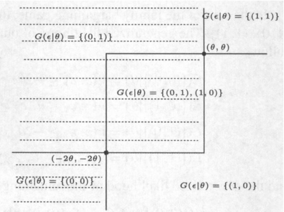
(b) Inequality to check

Figure 1. Family Game

The model thus described is incomplete in the sense that more information is required in the regions of multiplicity to determine which equilibrium will be selected. Without knowledge of such an equilibrium selection mechanism, the likelihood predicted by the model can be written as follows. As before $\mathcal{Y}$ denotes the set of possible outcomes. The likelihood of observation $y$ is $\mathcal{L}(y|\theta)=\nu(\epsilon:\;y\in G(\epsilon|\theta)|\theta)=\nu(G^{-1}(y|\theta)|\theta)$, for all $y\in\mathcal{Y}$ and $\sum_{y\in\mathcal{Y}}\mathcal{L}(y|\theta)\geq 1$, where the inequality may be strict if there are regions of multiplicity.

• In the case of the family bargaining game, the set of possible outcomes is $\mathcal{Y}=\{(0,0)$, $(0,1)$, $(1,0)$, $(1,1)\}$. The likelihood of outcomes predicted by the model can be written as follows.

  $$\mathcal{L}(\{(0,0)\}|\theta)=\nu(\epsilon:\;\epsilon_{1}\leq-2\theta,\;\epsilon_{2}\leq-2\theta|\theta)=\nu(G^{-1}((0,0)|\theta)|\theta)$$

  $$\mathcal{L}(\{(0,1)\}|\theta)=\nu(\epsilon:\;\epsilon_{1}\leq\theta,\;\epsilon_{2}\geq-2\theta|\theta)=\nu(G^{-1}((0,1)|\theta)|\theta)$$

  $$\mathcal{L}(\{(1,0)\}|\theta)=\nu(\epsilon:\;\epsilon_{1}\geq-2\theta,\;\epsilon_{2}\leq\theta|\theta)=\nu(G^{-1}((1,0)|\theta)|\theta)$$

  $$\mathcal{L}(\{(1,1)\}|\theta)=\nu(\epsilon:\;\epsilon_{1}\geq\theta,\;\epsilon_{2}\geq\theta|\theta)=\nu(G^{-1}((1,1)|\theta)|\theta)$$

  and the likelihood of the remaining events can be derived as follows

  $$\mathcal{L}(\{(0,0)\}\cup A|\theta)=\mathcal{L}(\{(0,0)\}|\theta)+\mathcal{L}(A|\theta),\;\mbox{ for all }\;A\subseteq\mathcal{Y}\backslash\{(0,0)\}$$

  $$\mathcal{L}(\{(1,1)\}\cup A|\theta)=\mathcal{L}(\{(1,1)\}|\theta)+\mathcal{L}(A|\theta),\;\mbox{ for all }\;A\subseteq\mathcal{Y}\backslash\{(1,1)\}$$

  $$\mathcal{L}(\{(0,1),(1,0)\}|\theta)=1-\mathcal{L}(\{(0,0),(1,1)\}|\theta)$$

  The likelihood predicted by the model is the set function $A\mapsto\mathcal{L}(A|\theta)=\nu(G^{-1}(A|\theta)|\theta)$ for $A$ subset of $\mathcal{Y}=\{(0,1)$, $(0,1)$, $(1,0)$, $(1,1)\}$. This set function is a Choquet capacity and if the support of $\nu$ is sufficiently large, the likelihood sums to more than one, because the region of multiple equilibria is “counted twice”. This is related to the non-additive feature of Choquet capacities, as seen here with the inequality $\nu(G^{-1}(\{(0,1)\}\cup\{(1,0)\}|\theta)|\theta)<\nu(G^{-1}(\{(0,1)\}|\theta)|\theta)+\nu(G^{-1}(\{(1,0)\}|\theta)|\theta)$, since the latter is equal to the former plus $\nu(\epsilon:\;-2\theta\leq\epsilon_{1}\leq\theta,-2\theta\leq\epsilon_{2}\leq\theta|\theta)$.

The model can be completed by adding an equilibrium selection mechanism which will pick out a single equilibrium for each value of the latent variable $\epsilon$ in the region of multiplicity. As formally defined in the previous section, an equilibrium selection mechanism is a conditional probability $\pi(.|\epsilon,X)$ with support included in $G(\epsilon|X;\theta)$. It is compatible with the data if the probabilities it predicts are equal to the true probabilities of the observable variables.

• In the family bargaining example example, we have for $i,j=0,1$:

  $$P((i,j)|X)=\int_{\mathcal{U}}\pi((i,j)|\epsilon,X)\nu(d\epsilon|X;\theta)$$

As noted above, since the model contains no prior information about which outcome is selected in the regions of multiplicity, the identified set $\Theta_{I}$ for the parameter vector $\theta$ is the set of parameters for which one can find an equilibrium selection mechanism which completes the model and equates probabilities of outcomes predicted by the model with true outcome frequencies. The definition of the identification region using a semiparametric likelihood representation, where the equilibrium selection mechanism is included as the infinite dimensional nuisance parameter $\pi$ is impractical, so we use theorem 1 to provide an operational method to compute $\Theta_{I}$. The existence of a compatible selection mechanism is equivalent to the fact that the true distribution $P$ of observed outcomes lies in the core of the Choquet capacity $\mathcal{L}=\nu G^{-1}$ defined by the model. Hence, we have $\Theta_{I}=\{\theta\in\Theta:\;\left(\forall A\in 2^{\mathcal{Y}};\;P(A|X)\leq\mathcal{L}(A|X;\theta);\right)\;X\,\mathrm{a.s.}\}$ where $2^{S}$ denotes the set of all subsets of a set $S$.

• In the case of the family bargaining game, the identified region is the set of parameter vectors that satisfy the 16 inequalities $P(A)\leq\nu(G^{-1}(A|\theta)|\theta)$ for all sets $A$ in $2^{\mathcal{Y}}$. Figure 1(b) gives a representation of one of the inequalities to be checked. The probability of the outcome being either $(0,0)$ or $(0,1)$ needs to be no larger than the probability of the latent variable lying in the set covered with horizontal dashed lines.

2. Efficient computation of the identified set: which inequalities to check, and how to check them?

We now describe three approaches to the effective computation of the identified set based on our characterization of theorem 1.

The first approach, described in section 2.1 is based on the observation that the likelihood is a submodular set function (the set function analogue of a convex function), and that checking the condition of theorem 1 is equivalent to minimizing a submodular function, which is a well studied problem (analogous to minimizing a convex function) and easily and efficiently implementable. It extends readily to the more general case when equilibria in mixed strategies are also allowed, as will be discussed in the computational part of section 4.

The second approach, described in section 2.2, is a special case of the first, which relies on the highly efficient algorithms (and easily available packaged implementations) for optimal transportation problems. As a combinatorial optimization method, it is a well known special case of the second approach, and it is computationally more efficient, and therefore recommended to practitioners who restrict attention to equilibria in pure strategies.

The third approach, based on the notion of core determining classes of sets and providing a dramatic reduction in the computational complexity under specific assumptions on the game under study, is described in section 2.3, where it is shown how the exponential problem of checking $2^{|\mathcal{Y}|}-2$ inequalities in theorem 1 can be replaced by the problem polynomial problem of checking $2|\mathcal{Y}|-2$ inequalities instead.

2.1. Submodular optimization

The first proposal to deal with the complexity of the problem of checking inequalities in theorem 1 is a method of general validity based on the minimization of a submodular function, the discrete equivalent of a convex function, which is a well known problem in combinatorial optimization, and for which efficient algorithms and easily available off the shelf implementations exist.

Definition 6 (Submodular function).

A set function $\mathcal{L}:\mathcal{Y}\rightarrow\mathbb{R}$ is called submodular if for each $A,B\subseteq\mathcal{Y}$, we have $\mathcal{L}(A\cup B)+\mathcal{L}(A\cap B)\leq\mathcal{L}(A)+\mathcal{L}(B)$. Note that in the special case where $\mathcal{L}$ is a probability measure, the latter inequality holds as an equality.

Submodularity for set functions is the analogue of convexity, and the problem of minimizing a submodular function is well studied (see for instance [50] chapter 2). A complete account of the theory can be found in [24] and off the shelf matlab implementation of the most efficient known algorithms can be found in Andreas Krause’s SFO toolbox.

We now show that checking inequalities involved in the characterization of the identified set in theorem 1 is indeed equivalent to the minimization of a submodular function. Theorem 1 shows that the identified set is the set of values of $\theta$ such that $X$-almost surely, we have the domination $\forall A\subseteq\mathcal{Y}$, $P(A|X)\leq\mathcal{L}(A|X;\theta)$, or equivalently $\min_{A\subseteq\mathcal{Y}}\left(\mathcal{L}(A|X;\theta)-P(A|X)\right)\geq 0$. We first note that the function in the minimization above is indeed submodular.

Lemma 1 (Submodularity of the likelihood).

For all $\theta\in\Theta$, $X$-almost surely, the set function on $\mathcal{Y}$ defined for all $A\subseteq\mathcal{Y}$ by $A\mapsto\mathcal{L}(A|X;\theta)-P(A|X)$ is submodular.

The most efficient generic way to check that a convex function is everywhere non negative is to minimize it and to verify that the minimum is non negative. In the same way, we propose to check inequalities of theorem 1 by minimizing the submodular function defined for all $A\subseteq\mathcal{Y}$ by $A\mapsto\mathcal{L}(A|X;\theta)-P(A|X)$, and checking that the minimum is indeed non negative. Of course, we can speed up the algorithm by stopping short of the minimum as soon as a negative value is found.

Theorem 2 (Computation of the identified set).

The identified set is obtained by minimization of a submodular set function: $\Theta_{I}=\left\{\theta\in\Theta:\;\min_{B\subseteq\mathcal{Y}}\left(\mathcal{L}(B|X;\theta)-P(B|X)\right)=0,\;X-\mbox{a.s.}\right\}$.

More details of the procedure are given in section 4, as this method is one of the recommended methods of construction of the identified set in the case where equilibria in mixed strategies are considered. Below is a description of a special case of submodular optimization, which is more efficient, and applies to the case where only equilibria in pure strategies are considered.

2.2. Optimal transportation approach

In the special case with only pure strategy equilibria that we are considering until section 4, the model likelihood $\mathcal{L}$ is a very special case of submodular function, since it is derived as the distribution function of a random set, or random correspondence $\mathcal{L}(A|X;\theta)=\nu(\epsilon:\;G(\epsilon|X;\theta)\cap A\neq\varnothing|X;\theta)$. It is that property that allows the following refinement of the method, and the simpler and more efficient technique proposed below. When mixed equilibria are considered, this improvement in efficiency is no longer available, precisely because in general the model likelihood is no longer the distribution of a random set.

To describe the method, we need the following notations and definitions. The terminology used is intended to be self-explanatory. Otherwise, the reader is referred to [42] for standard definitions in graph theory. Call $\mathcal{U}^{\ast}$ the set of predicted combinations of equilibria, formally $\mathcal{U}^{\ast}=\{G(\epsilon|X;\theta);\epsilon\in\mathcal{U}\}$ (we suppress reference to the dependence of $\mathcal{U}^{\ast}$ on $\theta$ for notational convenience). Hence $\mathcal{U}^{\ast}$ contains subsets of $\mathcal{Y}$, but is typically of much lower cardinality than the power set $2^{\mathcal{Y}}$. Further consider the bi-partite graph $\mathcal{G}(\theta,X)$ in $\mathcal{Y}\times\mathcal{U}^{\ast}$. The latter is defined as the set of pairs $(y,u)\in\mathcal{Y}\times\mathcal{U}^{\ast}$ such that $y\in u$. Each vertex $y$ in $\mathcal{Y}$ has weight $\mathbb{P}(Y=y|X)$ and each vertex $u\in\mathcal{U}^{\ast}$ has weight $\mathbb{P}(G(\epsilon|X;\theta)=u|X)$. The graph contains edges $(y,u)$ linking an element $y\in\mathcal{Y}$ to an element $u\in\mathcal{U}^{\ast}$ if the former is an element of the latter (i.e. $y\in u$). Finally, call $P(y|X)=\mathbb{P}(Y=y|X)$ the actual probabilities of observable variables $y\in\mathcal{Y}$, and call $Q(.|X;\theta)$ the probabilities $Q(u|X;\theta)=\mathbb{P}(G(\epsilon|X;\theta)=u|X)$. If we consider $G$ (keeping the same notation for simplicity) as a correspondence from $\mathcal{U}^{\ast}$ to $\mathcal{Y}$, then, formally $G(u)=u$, and we have shown in theorem 1 that $\theta$ belongs to the identified set if and only if for any subset $A$ of $\mathcal{Y}$, $P(A|X)\leq Q(G^{-1}(A)|X;\theta)$. [27] show that it is equivalent to the existence of a joint probability $\pi$ on $\mathcal{G}(\theta,X)$ with marginal distributions $P(.|X)$ and $Q(.|X;\theta)$. This is summarized in the following proposition.

Theorem 3.

The parameter value $\theta$ belongs to the identified set if and only if there exists a probability on $\mathcal{Y}\times\mathcal{U}^{\ast}$ with domain $\mathcal{G}(X;\theta)$ and with marginal probabilities $P(.|X)$ and $Q(.|X;\theta)$.

Note that one implication in theorem 3 is very easy to prove. Call $U$ the random element with distribution $Q$. If a joint probability exists with the required properties, then ${Y\in A}\Rightarrow U\in G^{-1}(A)$, so that $1_{\{Y\in A\}}\leq 1_{\{U\in G^{-1}(A)\}}$, $\pi$-almost surely. Taking expectation, we have $\mathbb{E}_{\pi}(1_{\{Y\in A\}})\leq\mathbb{E}_{\pi}(1_{\{U\in G^{-1}(A)\}})$, or equivalently $P(A|X)\leq Q(G^{-1}(A))|X;\theta)$. The converse is much more involved and relies on optimal transportation theory. A similar result is proved in theorem 3 of [4], based on an extension of the marriage lemma.

We illustrate this requirement on our example 1.2.2.

• For the case of the family bargaining game, $\mathcal{U}^{\ast}=\large\{\{(0,0)\}$, $\{(0,1)\}$, $\{(1,0)\}$, $\{(1,1)\}$, $\{(0,1),(1,0)\}\large\}$. The bi-partite graph representing the admissible connections between observable outcomes and combinations of equilibria is shown in figure 2(a), where $p_{y}$ denotes $\mathbb{P}(Y=y|X)$ and $q_{u}=\mathbb{P}(G(\epsilon|X;\theta)=u|X)$. The existence of a joint probability on $\mathcal{Y}\times\mathcal{U}^{\ast}$ supported on $\mathcal{G}(X;\theta)$ with marginal probabilities $p_{y}$, $y\in\mathcal{Y}$ and $q_{u}$, $u\in\mathcal{U}^{\ast}$ can be represented graphically by a set of non negative numbers attached to each edge of the graph, that sum to 1, and such that the weight of each vertex is equal to the sum of the weights on the edges that reach it. For instance, a joint probability is denoted $\alpha_{y}^{u}$, $(y,u)\in\mathcal{Y}\times\mathcal{U}^{\ast}$ and must satisfy $\alpha_{y}^{u}\geq 0$ for all $(y,u)\in\mathcal{Y}\times\mathcal{U}^{\ast}$, $\alpha_{y}^{u}=0$ if $y\notin u$, $\sum_{y\in u}\alpha_{y}^{u}=1$ and equalities such as $p_{01}=\alpha_{01}^{01}+\alpha_{01}^{01,10}$ and $q_{01,10}=\alpha_{01}^{01,10}+\alpha_{10}^{01,10}$.

Figure 2. Family game (continued)

Since we have now formulated the problem of computing the identified set as a problem involving the existence of a probability measure with given marginal distributions, we can appeal to efficient computational methods in the optimal transportation literature. The problem of sending $p_{y}$, $y\in\mathcal{Y}$ units of a good from sources $y\in\mathcal{Y}$ to $q_{u}$, $u\in\mathcal{U}^{\ast}$ units in terminals $u\in\mathcal{U}^{\ast}$ at minimum cost of transportation, where costs are attached to each pair $(y,u)\in\mathcal{Y}\times\mathcal{U}^{\ast}$ is called an optimal transportation problem, and first appears in the economics literature with [35]. Our problem can be reduced to an optimal transportation problem with 0-1 cost of transportation, where a pair $(y,u)$ is assigned cost zero if it belongs to $\mathcal{G}(X;\theta)$, and 1 otherwise, and there exists a joint law on $\mathcal{G}(X;\theta)$ with marginals $P$ and $Q$ (in other words, $\theta$ is in the identified set) if and only if there is a zero cost solution to the optimization problem thus defined.

As explained in [23] (see also [42] section 7.4 page 143), there is an equivalent dual formulation of this minimum cost of transportation problem as a maximum flow problem described in figure 2(b). The edges in the graph with zero cost in the minimum cost of transportation problem have infinite carrying capacity (not to be confused with Choquet capacity) in the dual maximal flow problem. Hence efficient maximum flow programs (such as maxflow.m in the Matlab BGL library) can be applied directly to the network described in figure 2(b): Mass flows from the source to the sink through the network. The number on each edge is the maximum mass that can flow through that edge. The source sends $p_{y}$ mass exactly to each node corresponding to elements of $\mathcal{Y}$, and the sink receives $q_{u}$ mass from each node corresponding to an element of $\mathcal{U}^{\ast}$. Between edges in $\mathcal{Y}$ and $\mathcal{U}^{\ast}$, mass can flow freely through pairs $(y,u)$ such that $y\in u$ (full lines with infinite carrying capacity), and not at all through pairs $(y,u)$ such that $y\notin u$. The parameter value $\theta$ is in the identified set if and only if the maximum flow program returns a maximum flow of exactly $1$ (note that the network carrying capacities depend on $\theta$ through the probabilities $q_{u}$). The full procedure is described in detail on the oligopoly entry example of section 3.

2.3. Core determining classes

As we have seen in the first section, theorem 1 allows to reduce the problem of computing the identified set to that of checking a set of inequalities. However, the computational burden is only partially lifted, as the number of inequalities to check can be very large if the cardinality of the outcome space is large. In this section, we shall analyze ways of reducing this remaining computational burden, by eliminating redundant inequalities in the computation of the identified set. This is formalized with the concept of core determining classes, which was first introduced in section 3.2.2 page 27 of [26].

Definition 7.

A class $\mathcal{A}$ of measurable subsets of $\mathcal{Y}$ is called core determining for the Choquet capacity $\mathcal{L}$ on $\mathcal{Y}$ if it is sufficient to characterize the core of $\mathcal{L}$, i.e. if a probability $Q$ is in $\mathrm{core}(\mathcal{L})$ when $Q(A)\leq\mathcal{L}(A)$ for all $A\in\mathcal{A}$. In other words, $Q(A)\leq\mathcal{L}(A)$ for all $A\in\mathcal{A}$ implies $Q(A)\leq\mathcal{L}(A)$ for all $A$ measurable.

A core determining class $\mathcal{A}$ allows the elimination of all the inequalities $Q(A)\leq\mathcal{L}(A)$ for $A\notin\mathcal{A}$ when checking whether a probability $Q$ belongs to the core of a Choquet capacity $\mathcal{L}$. Since the likelihood predicted by the model $Y\in G(\epsilon|X;\theta)$ was characterized by the Choquet capacity $A\mapsto\mathcal{L}(A|X;\theta)=\nu(\epsilon:G(\epsilon|X;\theta)\cap A\neq\varnothing|X;\theta)$, a core determining class of sets is sufficient to characterize the identified region $\Theta_{I}$ as summarized in the following proposition.

Proposition 1.

If $\mathcal{A}$ is core determining for the Choquet capacity $A\mapsto\mathcal{L}(A|X;\theta)=\nu(\epsilon:G(\epsilon|X;\theta)\cap A\neq\varnothing|X;\theta)$ $X$-almost surely, and for all $\theta$, then $\Theta_{I}=\{\theta\in\Theta:\forall A\in\mathcal{A}(\theta),\,P(A|X)\leq\mathcal{L}(A|X),\,X-\mathrm{a.s.}\}$.

The challenge therefore becomes that of finding a core determining class $\mathcal{A}$ in order to reduce the number of inequalities to be checked to the cardinality of $\mathcal{A}$. We first consider the case of our example 1.2.2, before turning to a criterion that will prove useful in exhibiting core determining classes in many important cases.

• We return to the family bargaining game and consider some proposals for the computation of the identified set proposed in the literature. We call Singleton class the class of singleton sets $(\{(0,0)\}$, $\{(0,1)\}$, $\{(1,0)\}$, $\{(1,1)\})$, since it corresponds to the class of sets proposed in [2] specialized to this simple case. It is immediate to see that the Singleton class is not core determining in general. Indeed, if $\epsilon$ has large enough support, the two equalities $P(\{(0,1)\})=\nu(G(\epsilon|\theta)\cap\{(0,1)\}\neq\varnothing|\theta)=\nu(\epsilon:\;\epsilon_{1}\leq\theta,\;\epsilon_{2}\geq-2\theta|\theta)$ and $P(\{(1,0)\})=\nu(G(\epsilon|\theta)\cap\{(1,0)\}\neq\varnothing|\theta)=\nu(\epsilon:\;\epsilon_{1}\geq-2\theta,\;\epsilon_{2}\leq\theta|\theta)$ jointly imply $P(\{(0,1),(1,0)\})>\nu(G(\epsilon|\theta)\cap\{(0,1),(1,0)\}\neq\varnothing|\theta)=\nu(\epsilon:\;[\epsilon_{1}\geq-2\theta\,\mathrm{or}\,\epsilon_{2}\geq-2\theta]\,\mathrm{and}\;[\epsilon_{1}\leq\theta\,\mathrm{or}\,\epsilon_{2}\leq\theta]|\theta)$.

We now show how to identify core determining classes more generally to avoid painstaking case-by-case elimination of redundant inequalities. To that end, we give general conditions under which one can find a core determining class of low cardinality. Recall that a subset $A$ of an ordered set (with ordering $\preceq$) is said to be connected if any $a$ such that $\inf A\preceq a\preceq\sup A$ belongs to $A$.

Assumption 2 (Monotonicity).

There exists an ordering $\precsim_{\mathcal{Y}}$ of the set of outcomes $\mathcal{Y}$ and an ordering $\precsim_{\mathcal{U}}$ of the set of latent variables $\mathcal{U}$ such that $G(\epsilon|X;\theta)$ is connected for all $\epsilon\in\mathcal{U}$, $X$-a.s., all $\theta$, and $\sup G(\epsilon_{2}|X;\theta)\succsim_{\mathcal{Y}}\sup G(\epsilon_{1}|X;\theta)$ and $\inf G(\epsilon_{2}|X;\theta)\succsim_{\mathcal{Y}}\inf G(\epsilon_{1}|X;\theta)$ when $\epsilon_{1}\precsim_{\mathcal{U}}\epsilon_{2}$. Both ordering are allowed to depend on the exogenous variables $X$, but the dependence is suppressed in the notation for clarity.

Remark 1.

This assumption is related to monotone comparative statics in supermodular games (see [50], [51] and [39]).

We illustrate this assumption on our family bargaining game before stating the theorem and applying it to the more sophisticated case of an oligopoly entry game with two types of players presented in [9].

• In the family bargaining game, the orderings are very simple to construct. A lexicographic order on $\mathcal{Y}$ is suitable, with $(0,0)\precsim_{\mathcal{Y}}(0,1)\precsim_{\mathcal{Y}}(1,0)\precsim_{\mathcal{Y}}(1,1)$. On $\mathcal{U}$ the ordering is related to predicted outcomes. All $\epsilon$ producing the same predicted outcomes will be equivalent, and the ordering on predicted outcomes is $\{(0,0)\}\precsim_{\mathcal{U}}\{(0,1)\}\precsim_{\mathcal{U}}\{(0,1),(1,0)\}\precsim_{\mathcal{U}}\{1,0\}\precsim_{\mathcal{U}}\{1,1\}$, where $A_{1}\precsim_{\mathcal{U}}A_{2}$ is a short-hand notation for $\epsilon_{1}\precsim_{\mathcal{U}}\epsilon_{2}$ if $G(\epsilon_{1}|X;\theta)=A_{1}$ and $G(\epsilon_{2}|X;\theta)=A_{2}$. It is straightforward to check assumption 2. For instance, taking $\epsilon_{1}$ such that $G(\epsilon_{1}|\theta)=\{(0,1)\}$ and $\epsilon_{2}$ such that $G(\epsilon_{2}|\theta)=\{(0,1),(1,0)\}$ we have $\sup G(\epsilon_{1}|\theta)=(0,1)\precsim_{\mathcal{Y}}(1,0)=\sup G(\epsilon_{2}|\theta)$ and $\inf G(\epsilon_{1}|\theta)=(0,1)=\inf G(\epsilon_{2}|\theta)$. This is illustrated in figure 3.

Figure 3. The monotonicity requirement in assumption 2 is satisfied for this choice of orderings in the family bargaining example. (The thick dots represent the correspondence $G(.|\theta)$). $\mathcal{U}^{\ast}$ denotes the ordered set of combinations of equilibria.

We are now in a position to state the theorem, which is the main tool in the construction of core determining classes, and hence in the computation of the identified set.

Theorem 4.

Suppose assumption 2 is satisfied with orderings $\precsim_{\mathcal{Y}}$ and $\precsim_{\mathcal{U}}$. Call $I$ the cardinality of $\mathcal{Y}$, and list outcomes (elements of $\mathcal{Y}$) in increasing order (with respect to ordering $\precsim_{\mathcal{Y}}$) as $y_{1},\ldots,y_{I}$. Then $\mathcal{A}=(\{y_{1},\ldots,y_{i}\},\{y_{i},\ldots,y_{I}\}:\;i=1\ldots,I)$ is core determining.

Theorem 4 allows to reduce the cardinality of the power set $2^{\mathcal{Y}}$ to twice the cardinality of $\mathcal{Y}$ minus $2$ (since the inequality needn’t be checked on the whole set $\mathcal{Y}$), as we illustrate in our example 1.2.2.

• In the family bargaining example, assumption 2 is satisfied, as seen on figure 3, with the ordering described above. Hence the class $\left(\{(0,0)\}\right.$, $\{(0,0),(0,1)\}$, $\{(0,0),(0,1),(1,0)\}$, $\{(0,1),(1,0),(1,1)\}$, $\{(1,0),(1,1)\}$, $\left.\{(1,1)\}\right)$ is core determining.

3. Illustration: oligopoly entry with two types of players

We now turn to a more substantive illustration of our methods to compute the identified set, first, to show the operational usefulness of corollary 4, and second, to illustrate the power of the combinatorial approach. To do so, we consider the oligopoly entry game with two types of players presented in appendix A of [9]. The profit function of type 1 firms depends on the total number of firms in the market, but not on the type of those firms, whereas profits of type 2 firms depend both on the number and on the type of firms present in the market. The latent variable is the fixed cost $f_{1}$ for firms of type 1 and $f_{2}$ for firms of type 2. $(f_{1},f_{2})$ is uniformly distributed over $[0,1]^{2}$. The model is simplified by assuming linearity of profits in firm number as follows.

$$\pi_{1}(Y_{1},Y_{2},X,f;\theta)=\alpha_{0}+\alpha_{1}(Y_{1}+Y_{2})+\alpha_{2}X-f_{1}$$

$$\pi_{2}(Y_{1},Y_{2},X,f;\theta)=\beta_{0}+\beta_{1}Y_{1}+\beta_{2}Y_{2}+\beta_{3}X-f_{2},$$

with $\alpha_{1},\beta_{1},\beta_{2}$ strictly negative and $\beta_{2}>\beta_{1}$ to fix ideas (profit of type 2 firms will decrease by a larger amount if a type 1 firm enters the market than if a type 2 firm does). The set of observable outcomes is $\mathcal{Y}=\{(i,j):\;i,j=0,1,2\}$, where $i$ denotes the number of type 1 firms and $j$ the number of type 2 firms present in the market. $\mathcal{Y}$ can be ordered lexicographically, where the number of firms present in the market is considered first, and then the identity of firms (type 1 dominating type 2). Hence $(0,0)\precsim_{\mathcal{Y}}$ $(0,1)\precsim_{\mathcal{Y}}$ $(1,0)\precsim_{\mathcal{Y}}$ $(0,2)\precsim_{\mathcal{Y}}$ $(1,1)\precsim_{\mathcal{Y}}$ $(2,0)\precsim_{\mathcal{Y}}$ $(1,2)\precsim_{\mathcal{Y}}$ $(2,1)\precsim_{\mathcal{Y}}$ $(2,2)$. The model correspondence is represented in figure 4, which is taken from [9].

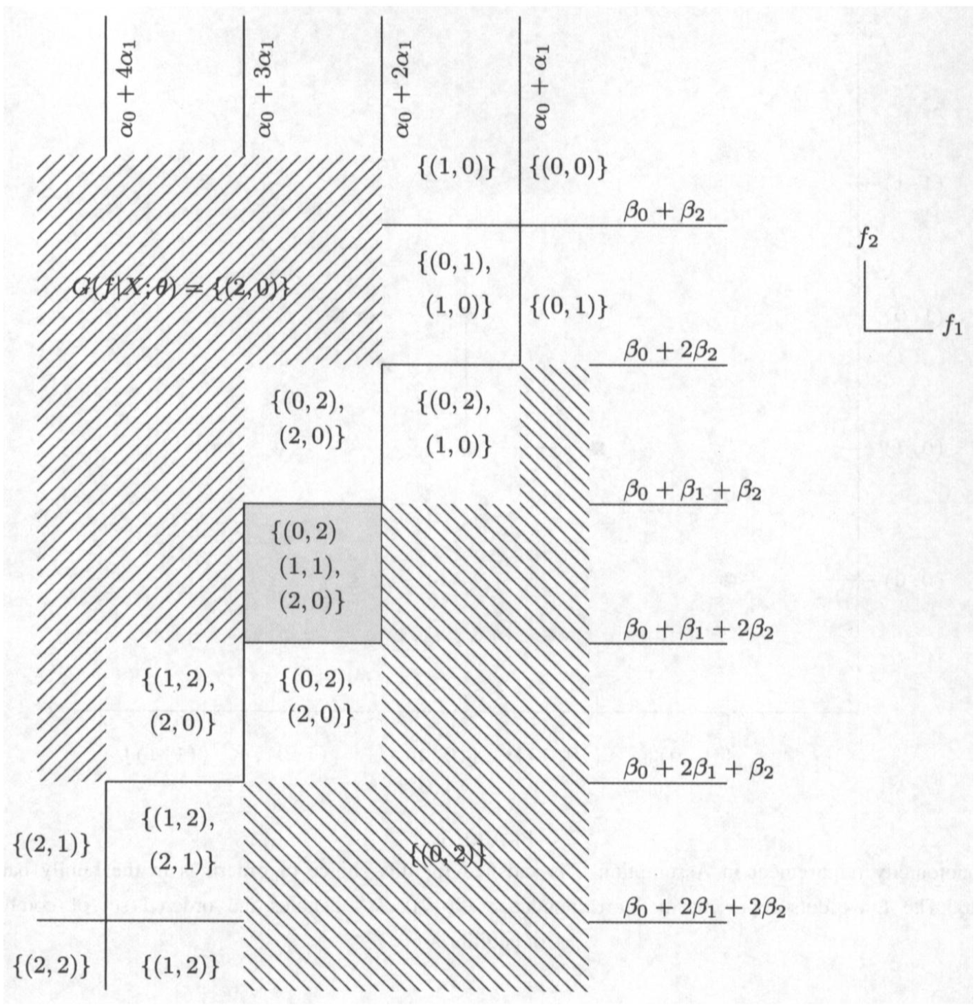
Figure 4. Model correspondence in the oligopoly entry game with two types of firms, two of each type.

3.1. Submodular optimization approach

The implementation of the submodular optimization method is extremely simple. Once the values of the likelihood have been derived (analytically in the present case, but more often by simulation following the method proposed in [5]), all that remains to do to check whether a value $\theta$ belongs to the identified set, is to minimize the function defined for all $A\subseteq\mathcal{Y}$ by $A\mapsto\mathcal{L}(A|X;\theta)-P(A|X)$ using for instance the Matlab SFO toolbox routine $SFO-min-norm-point.m$ implementing Fujishige’s algorithm (see page 293 of [24]).

3.2. Optimal transportation approach

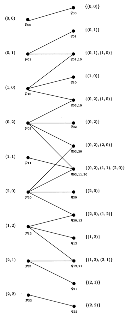
Figure 8. Bi-partite graph representing the admissible connections between observable outcomes and combinations of equilibria in the two-type oligopoly entry model.

Consider now the linear programming strategy for computing the identified set. The bipartite graph corresponding to this example is represented in figure 8.

As shown in theorem 3, a value of the parameter vector is in the identified set if and only if there exists a zero cost transportation plan for the transfer of masses $p_{y}$ on the elements of $\mathcal{Y}$ to masses $q_{u}$ on the elements of $\mathcal{U}^{\ast}$. A transportation plan is a set of nonnegative numbers attached to all pairs $(y,u)\in\mathcal{Y}\times\mathcal{U}^{\ast}$ (which represents the amount of mass from $y$ that is transferred to $u$ via the edge $(y,u)$). In our application, the transportation cost from $y$ to $u$ is zero if $y$ and $u$ are connected by an edge in the graph of figure 8, and 1 otherwise. If the algorithm returns a zero cost transportation plan, it means that mass is transferred through edges of the graph only, and for instance the pair $\left((1,1),\{(0,2),(1,1),(2,0)\}\right)$ is assigned a non negative number (i.e. some mass is transported there), but the pair $((1,1),\{(2,0),(0,2)\})$ is assigned zero (i.e. no mass is transported there). The existence of a zero cost transportation plan is equivalent to the existence of a joint distribution on $\mathcal{Y}\times\mathcal{U}^{\ast}$ which is supported on the graph of figure 8 and has the correct marginal distributions, hence, it is equivalent to the fact that $\theta$ is in the identified set, as we showed in theorem 3.

The minimum cost transportation problem is equivalent to the dual maximum flow problem, as described in the previous section. Mass flows through the network with $25$ nodes, which include the source, the $9$ elements of $\mathcal{Y}$, the $14$ elements of $\mathcal{U}^{\ast}$ and the sink (mass flows in the direction $\mathrm{Source}\rightarrow\mathcal{Y}\rightarrow\mathcal{U}^{\ast}\rightarrow\mathrm{Sink}$). A network is characterized by its adjacency matrix, which gives all the links between nodes with their capacity. In the case of interest here, the adjacency matrix is given in table 2. Maximum flow programs take this adjacency matrix as an input, and return the maximum flow through the network it characterizes. This maximum flow cannot be larger than $\sum_{y\in\mathcal{Y}}p_{y}=\sum_{u\in\mathcal{U}^{\ast}}q_{u}=1$, and it is equal to $1$ if and only if $\theta$ is in the identified set.

3.3. Core determining class approach

We now illustrate the usefulness of corollary 4 for the determination of a core determining class in this example. Figure 5 graphs the orderings that satisfy assumption 2 up to the fact that the set of equilibria is not always connected. Indeed, in the ordering of outcomes, $(1,1)$ comes between $(0,2)$ and $(2,0)$, or more precisely, $(0,2)\precsim_{\mathcal{Y}}(1,1)\precsim_{\mathcal{Y}}(2,0)$. Now $(1,1)$ is not an equilibrium when $\alpha_{0}+3\alpha_{1}<f_{1}\leq\alpha_{0}+2\alpha_{1}$ and $\beta_{0}+\beta_{1}+\beta_{2}<f_{2}\leq\beta_{0}+2\beta_{2}$, so the set of equilibria $\{(0,2),(2,0)\}$ is disconnected in that case.

Figure 5. Assumption 2 is satisfied in the oligopoly entry game with two types of firms, two of each type, up to the fact that the image of $G(\{(0,2),(2,0)\}|X;\theta)$ is not connected.

However, since $(1,1)$ is observed only when $\epsilon\in\{(0,2),(1,1),(2,0)\}$, the mass $p_{11}$ can be removed from $q_{02,11,20}$. Indeed, $(1,1)$ is isolated in the sense that all its mass is necessarily transferred to $\{(0,2),(1,1),(2,0)\}$, which is the only predicted combination of equilibria in which it appears. Hence, after checking that $p_{11}\leq q_{02,11,20}$, we can remove $p_{11}$ and $q_{02,11,20}$ and replace $q_{02,20}$ by $q_{02,20}+q_{02,11,20}-p_{11}$. Then, the monotonicity and connectedness conditions hold, and theorem 4 can be applied directly to $\mathcal{Y}\backslash\{(1,1)\}$ and $\mathcal{U}^{\ast}$, yielding the class $\mathcal{A}$ $=(\{(0,0)\},$ $\{(0,0),$ $(0,1)\},$ $\{(0,0),$ $(0,1),$ $(1,0)\},$ $\{(0,0),$ $(0,1),$ $(1,0),$ $(0,2)\},$ $\{(0,0),$ $(0,1),$ $(1,0),$ $(0,2),$ $(2,0)\},$ $\{(0,0),$ $(0,1),$ $(1,0),$ $(0,2),$ $(2,0),$ $(1,2)\},$ $\{(0,0),$ $(0,1),$ $(1,0),$ $(0,2),$ $(2,0),$ $(1,2),$ $(2,1)\},$ $\{(0,1),$ $(1,0),$ $(0,2),$ $(2,0),$ $(1,2),$ $(2,1),$ $(2,2)\},$ $\{(1,0),$ $(0,2),$ $(2,0),$ $(1,2),$ $(2,1),$ $(2,2)\},$ $\{(0,2),$ $(2,0),$ $(1,2),$ $(2,1),$ $(2,2)\},$ $\{(2,0),$ $(1,2),$ $(2,1),$ $(2,2)\},$ $\{(1,2),$ $(2,1),$ $(2,2)\},$ $\{(2,1),$ $(2,2)\},$ $\{(2,2)\})$. Note that its cardinality is $2\times 7=14$, as opposed to the cardinality of the power set of $\mathcal{Y}$ which is $2^{9}=512$.

Table 2. Adjacency matrix for the two-type oligopoly model.

	$(0,0)$	$(0,1)$	$(1,0)$	$(0,2)$	$(1,1)$	$(2,0)$	$(1,2)$	$(2,1)$	$(2,2)$	Sink
Source	$p_{00}$	$p_{01}$	$p_{10}$	$p_{02}$	$p_{11}$	$p_{20}$	$p_{12}$	$p_{21}$	$p_{22}$
$\{(0,0)\}$	$\infty$									$q_{00}$
$\{(0,1)\}$		$\infty$								$q_{01}$
$\{(0,1),(1,0)\}$		$\infty$	$\infty$							$q_{01,10}$
$\{(1,0)\}$			$\infty$							$q_{10}$
$\{(1,0),(0,2)\}$			$\infty$	$\infty$						$q_{02,10}$
$\{(0,2)\}$				$\infty$						$q_{02}$
$\{(0,2),(2,0)\}$				$\infty$		$\infty$				$q_{02,20}$
$\{(0,2),(1,1),(2,0)\}$				$\infty$	$\infty$	$\infty$				$q_{02,11,20}$
$\{(2,0)\}$						$\infty$				$q_{20}$
$\{(2,0),(1,2)\}$						$\infty$	$\infty$			$q_{20,12}$
$\{1,2\}$							$\infty$			$q_{12}$
$\{(1,2),(2,1)\}$							$\infty$	$\infty$		$q_{12,21}$
$\{(2,1)\}$								$\infty$		$q_{21}$
$\{(2,2)\}$									$\infty$	$q_{22}$

3.4. Efficiency comparison of the combinatorial methods

As an illustration of the procedure, we compute the identified set for the two-type oligopoly model with the following distributional hypotheses and normalization restrictions. The fixed cost vector $(f_{1},f_{2})$ is assumed to be uniformly distributed on $[0,1]^{2}$. $\alpha_{0}$ and $\beta_{0}$ are set equal to $1$. As previously noted, we assume that monopoly profits are larger than oligopoly profits, and that a type two firm’s profit decreases more if a type one firm enters than a type two firm, hence $0>\alpha_{0}$ and $0>\beta_{2}>\beta_{1}$. We can therefore calculate the probabilities of each combination of equilibria $u\in\mathcal{U}^{\ast}$. These probabilities are computed in a Matlab program file available on request.

The values of the model likelihood are derived from these probabilities, and the function $\mathcal{L}(.|X;\theta)-P(.|X)$ is then minimized over all subsets of $\mathcal{Y}$ using the Matlab routine SFO-min-norm-point.m from the SFO toolbox. An idea of the computational efficiency of this procedure is given by the fact that an order of $10^{3}$ values of the parameter can be tested in one second on a standard laptop computer.

To implement the minimum cost of transportation/maximum flow method, the probabilities of each value of the equilibrium correspondence are entered together with the true frequencies of observable outcomes into the adjacency matrix of table 2 and the Matlab routine maxflow.m of the BGL library returns a flow of $1$ if the value of $\theta=(\alpha_{1},\beta_{1},\beta_{2})^{\prime}$ (used to compute the predicted probabilities) belongs to the identified set, and a flow strictly smaller than $1$ if it doesn’t. To give an idea of the efficiency of the method, we can test $10^{5}$ values of $\theta=(\alpha_{1},\beta_{1},\beta_{2})^{\prime}$ in less than a second on a standard portable computer. Hence this method is faster than the general submodular minimization method, but only applies to pure strategy equilibria.

Finally, the additional information yielded by the existence of a core determining class for this problem allows us to test a value of the parameter by a constrained submodular optimization, where the search is limited to the sets in the core determining class.

Figure 6. Projection of the identified set, and of the set characterized by the Singleton class on the $(\beta_{2},\alpha_{1})$ space. The projection of the identified set is a single point $(\beta_{2},\alpha_{1})=(-0.4,-0.25)$. The frequencies of observable variables are $(p_{00},p_{01},p_{10},p_{02},p_{11},p_{20},p_{12},p_{21},p_{22})=(0.1,0.15,0.15,0.1,0,0.5,0,0,0)$.

For illustration purposes, we compute the identified set for a given choice of the observable frequencies, namely $(p_{00},p_{01},p_{10},p_{02},p_{11},p_{20},p_{12},p_{21},p_{22})=(0.1,0.15,0.15,0.1,0,0.5,0,0,0)$, and compare it to the set obtained by imposing the inequality restrictions on the Singleton class only. The latter corresponds to the set of values of the parameters such that $p_{00}\leq q_{00}$, $p_{01}\leq q_{01}+q_{01,10}$, $p_{10}\leq q_{01,10}+q_{10}+q_{02,10}$, $p_{02}\leq q_{02,10}+q_{02}+q_{02,20}+q_{02,11,20}$, $p_{11}\leq q_{02,11,20}$, $p_{20}\leq q_{02,20}+q_{02,11,20}+q_{20}+q_{20,12}$, $p_{12}\leq q_{20,12}+q_{12}+q_{12,21}$, $p_{21}\leq q_{12,21}+q_{21}$ and $p_{22}\leq q_{22}$. It turns out the values of $\alpha_{1}$ and $\beta_{2}$ are identified (under these specific values for the true probabilities of observable variables, which were chosen for the simulation purposes from the parameter values), and all values of $\beta_{1}<\beta_{2}$ are compatible with the given frequencies. The set defined by the Singleton class restrictions, however, is much larger, as shown by its projection on the $(\beta_{2},\alpha_{1})$ space in figure 6. There are also many values of the observed frequencies, for which the identified set is empty, so that the model is rejected, but the set defined by the Singleton class restrictions is non-empty, so that it fails to reject the model.

4. Extension to equilibria in mixed strategies

We now show how our results extend to the case where mixed strategy equilibria are allowed. As before, we consider a game parameterized by the deterministic parameter vector $\theta$, a vector of covariates $X$ and unobserved heterogeneity parameter $\epsilon$ with distribution $\nu(.|X;\theta)$. The observable outcomes of the game are equilibrium actions profiles $Y$ whose realizations belong to the finite set $\mathcal{Y}$. Call $P(.|X)$ the true distribution of observable outcomes $Y$ conditionally on $X$. The equilibrium correspondence $G(\varepsilon|X;\theta)$ is now the set of Nash equilibria of the game in mixed strategies (including pure strategies as degenerate mixed strategies). Call $\sigma$ the equilibrium strategy profile that is actually selected within the set $G(\epsilon|X;\theta)$, i.e. the model predicts $\sigma\in G(\epsilon|X;\theta)$. The outcome $Y$ is a random variable with distribution $\sigma$, so it can be written $Y=Q_{\sigma}(V)$, where $Q_{\sigma}$ is the quantile transform associated with $\sigma$, and $V$ is a random variable with uniform distribution, independent of $\epsilon$ and $\sigma$, conditionally on $X$. The variable $V$ is traditionally interpreted as an independent signal that agents receive and on whose realization they base their action. The identified set is therefore defined as the set $\Theta_{I}$ of values of the parameter such that $Y=Q_{\sigma}(V)$ and $\sigma\in G(\epsilon|X;\theta)$ as specified above.

Definition 8 (Identified set).

The identified set is equal to

$$\Theta_{I}=\left\{\theta\in\Theta:\;X-\mbox{a.s.},\;\exists(Y,\epsilon,\sigma,V):\;\right.$$

$$\left.\hskip 20.0ptY\sim P_{|X},\;\epsilon\sim\nu(.|X;\theta),\;V\sim U[0,1],\;Y=Q_{\sigma}(V),\;\sigma\in G(\epsilon|X;\theta),\;V\mathchoice{\mathrel{\hbox to0.0pt{$\displaystyle\perp$\hss}\mkern 2.0mu{\displaystyle\perp}}}{\mathrel{\hbox to0.0pt{$\textstyle\perp$\hss}\mkern 2.0mu{\textstyle\perp}}}{\mathrel{\hbox to0.0pt{$\scriptstyle\perp$\hss}\mkern 2.0mu{\scriptstyle\perp}}}{\mathrel{\hbox to0.0pt{$\scriptscriptstyle\perp$\hss}\mkern 2.0mu{\scriptscriptstyle\perp}}}\epsilon,\sigma\right\}$$

• We now return to the family bargaining game and derive the equilibrium correspondence $G(\epsilon|X;\theta)$, which is now a set of probabilities on $\mathcal{Y}$. We note that in addition to the equilibria appearing in figure 1(a), $\{(\frac{2\theta+\epsilon_{2}}{3\theta},\frac{2\theta+\epsilon_{1}}{3\theta})\}$ is a Nash equilibrium in mixed strategies if and only if $\theta>\epsilon_{1},\epsilon_{2}>-2\theta$. With the notational convention that $(\alpha,\alpha)$ corresponds to the equilibrium, where players independently participate with probability $\alpha$, we can represent the equilibrium correspondence as a function of $\epsilon$ in figure 7.

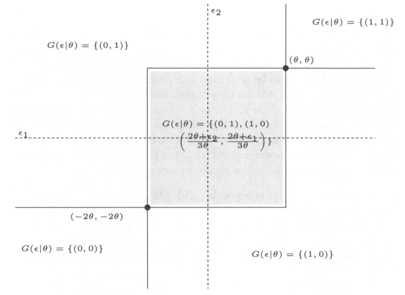
Figure 7. Model correspondence for the family bargaining case with mixed strategy equilibria.

[7] (hereafter BMM) were the first to extend the characterization of the identified set to the case of equilibria in mixed strategies, which is both a very important and nontrivial problem. It is particularly useful, as it is well known that in normal form games, existence of equilibria is guaranteed in mixed strategies, but not necessarily in pure strategies, except in special classes of games such as supermodular games. It is a nontrivial problem, since the likelihood of the model is no longer the distribution function of a random set. Nonetheless, we go beyond the results of BMM and show that in certain classes of games the identified set can be characterized by a finite set of inequalities. We also show that our efficient submodular optimization method is still applicable to this case, as the identified set continues to be characterized by the fact that true data distribution is contained in the core of the model likelihood as in theorem 1. In the general case, where the likelihood is not necessarily submodular, we show that the identified set can be computed efficiently through a convex optimization problem, which we describe.

We first show now that the identified set $\Theta_{I}$ defined in definition 8 is indeed equal to $\Theta_{I}^{\ast}$ defined in BMM. Indeed: suppose $\theta\in\Theta_{I}$. Call $\mu(.|\epsilon,X;\theta)$ the distribution of the random element $\sigma$ (hence a distribution on the simplex). The latter has support $G(\epsilon|X;\theta)$. Then, for any value $y\in\mathcal{Y}$, we have

$$P(Y=y|X) = \int\int P(Y=y|\epsilon,\sigma,X;\theta)d\mu(\sigma|\epsilon,X;\theta)d\nu(\epsilon|X;\theta)$$ (4.1)

$$= \int\int P(Q_{\sigma}(V)=y|\epsilon,\sigma,X;\theta)d\mu(\sigma|\epsilon,X;\theta)d\nu(\epsilon|X;\theta)$$

$$= \int\left(\int P_{\sigma}(Y=y|\epsilon,X;\theta)d\mu(\sigma|\epsilon,X;\theta)\right)d\nu(\epsilon|X;\theta)$$

by independence. Conversely, if (4.1) holds, we can construct the random quadruplet $(Y,V,\epsilon,\sigma)$ with the required properties.

The fundamental work by BMM was the first to derive a characterization of the identified set in the case of multiple mixed strategy equilibria, which we restate here as the following proposition:

Proposition 2 (BMM 2009).

$${\Theta_{I}=\left\{\theta\in\Theta:\;\forall f\;\mbox{ function on }\;\mathcal{Y}:E_{P}(f(Y)|X)\leq\tilde{\mathcal{L}}\left(f|X;\theta\right)\right\},}$$

where

$$\tilde{\mathcal{L}}\left(f|X;\theta\right){=}\int\left(\max_{\sigma\in G(\epsilon|X;\theta)}{E}_{\sigma}{(f(Y))}\right){d\nu(\epsilon|X;\theta),~{}f\;\mbox{ function on }\;\mathcal{Y}.}$$

For completeness, in the appendix we give a different proof of this result, as it fits more naturally with our presentation than the original random set theoretic proof given in [7]. We now show that this characterization allows efficient computation of the identified set as the solution of a convex optimization problem. In addition, under regularity conditions on the equilibrium correspondence of the game, we show that we can derive an exact characterization of the identified set with a finite collection of inequalities, as was the case when considering equilibria in pure strategies only.

4.1. Efficient computation

In this section, we give a simple procedure, which is valid for any normal form game, and is recommended to practitioners who do not wish to restrict attention to pure strategy Nash equilibria. In proposition 2, the functional $\tilde{\mathcal{L}}$ is convex, as a maximum of linear functionals. As a result, we show that the identified set can be computed with a standard convex optimization program. Indeed, $\Theta_{I}$ is the set of $\theta$’s such that the convex functional $\phi(f)=\tilde{\mathcal{L}}(f|X;\theta)-E_{P}(f(Y)|X)$ remains non negative for all function $f$. Suppose there is some $v$ (a function on $\mathcal{Y}$, hence a vector in $\mathbb{R}^{d_{y}}$) such that $\phi(v)<0$. Since $\phi$ is positively homogeneous (i.e. $\phi(\lambda v)=\lambda\phi(v)$ for all $\lambda\geq 0$), then for each $z\in\mathbb{R}^{d_{y}}$, such that $z\neq 0$, one of the following three cases applies:

• The inner product of $v$ with $z$ is negative, $\langle z,v\rangle<0$. Then setting $\lambda=-\langle z,v\rangle^{-1}$, we have $\langle z,\lambda v\rangle=-1$ and $\phi(\lambda v)=\lambda\phi(v)<0$, so that $\min_{\{w:\langle z,w\rangle=-1\}}\phi(w)<0$.

• The inner product of $v$ with $z$ is positive, $\langle z,v\rangle>0$. Then setting $\lambda=\langle z,v\rangle^{-1}$, we have $\langle z,\lambda v\rangle=1$ and $\phi(\lambda v)=\lambda\phi(v)<0$, so that $\min_{\{w:\langle z,w\rangle=1\}}\phi(w)<0$.

• The inner product is zero, $\langle z,v\rangle=0$. Then by convexity of $\phi$, there is a $\tilde{v}$ in the neighborhood of $v$ such that $\phi(\tilde{v})<0$ and $\langle z,\tilde{v}\rangle>0$.

Hence, if we take any $z$, for instance $z=(1,0,\ldots,0)$, and define $H=\{w:\langle z,w\rangle=0\}$, $\phi$ takes negative values if and only if the following statement is true

$$\min\left(\min_{w\in H}\phi(w+z),\hskip 5.0pt\min_{w\in H}\phi(w-z)\right)<0$$

Since $H$ is a convex set, the program above is a completely standard convex optimization program (we implement the procedure with the matlab optimization toolbox).

4.2. Cases with a submodular likelihood

We now turn to the efficient computation of the identified set in the case where the likelihood is submodular. This occurs when the game satisfies the following assumption, taken from [46]. Recall that the upper envelope $\phi$ of a family of probability functions $A\mapsto\mu_{i}(A)$, $i=1,\ldots,I$ is defined as $A\mapsto\phi(A)=\max_{i\in I}\mu_{i}(A)$.

Definition 9 (Regular core (Shapley)).

A normal form game is said to have a regular core if the upper envelope $A\mapsto\sup_{\sigma\in G}\sigma(A)$ of the equilibrium correspondence $G$ is submodular.

We now show a very simple and easy to check sufficient condition for a regular core.

Lemma 2 (Sufficient condition for a regular core).

A normal form game with multiple equilibria including only one equilibrium in proper mixed strategies and any number of equilibria in pure strategies has a regular core.

Remark 2.

Note that this sufficient condition is very easy to check, and it is satisfied for large classes of games (see [20] for games of strategic complementarities, and in particular $2\times 2$ games, when unstable equilibria are removed).

Theorem 5 (Characterization of the identified set).

If the game has a regular core for all $\theta$, $(X,\epsilon)$-almost surely, then

$$\Theta_{I}=\left\{\theta\in\Theta:\;\left(\forall B\subseteq\mathcal{Y}:P(B|X)\leq\mathcal{L}(B|X;\theta)\right);\;X-\mathrm{a.s.}\right\}$$

where

$$\mathcal{L}(B|X;\theta)=\int\left(\max_{\sigma\in G(\epsilon|X;\theta)}\sigma(B)\right)d\nu(\epsilon|X;\theta).$$

In this case, we give an exact characterization of the identified set with only a finite number of inequalities, unlike BMM’s characterization. One implication is trivial: it is obvious to see that $E_{P}{(f(Y)|X)\leq\tilde{\mathcal{L}}}\left(f|X;\theta\right)$ implies $P(B|X)\leq\mathcal{L}(B|X;\theta)$ (it suffices to take $f\left({y}\right)=1_{B}\left(y\right)$). The converse is far from trivial, and follows from the characterization of Choquet integrals (see [45]).

This implies that the problem of checking whether a value of the parameter is in the identified set is equivalent to the problem of checking whether the distribution of $Y$ is in the core of a Choquet capacity. This was already the case in [26] when we restricted ourselves to pure strategy equilibria. However, in the latter case, the Choquet capacity was infinitely alternating, as it was defined as the distribution of a random set. With mixed strategy equilibria, it no longer has this property, hence it is no longer the distribution of a random set.

• In the family bargaining example, the model likelihood can be derived in the following way: If the support of $\epsilon$ belongs to $[-2\theta,\theta]^{2}$, then

  • $\mathcal{L}(\{(0,1)\}|\theta)=\mathcal{L}(\{(1,0)\}|\theta)=1$

  • $\mathcal{L}(\{(0,0)\}|\theta)=\mathbb{E}_{\nu}[(\theta-\epsilon_{2})(\theta-\epsilon_{1})/(9\theta^{2})]$

  • $\mathcal{L}(\{(1,1)\}|\theta)=\mathbb{E}_{\nu}[(2\theta+\epsilon_{2})(2\theta+\epsilon_{1})/(9\theta^{2})]$

  • $\mathcal{L}(\{(1,1),(0,0)\}|\theta)=\mathcal{L}(\{(1,1)\}|\theta)+\mathcal{L}(\{(0,0)\}|\theta)$.

  The general case, where the domain of $\epsilon$ is unrestricted, can be deduced very simply from the above (see details in appendix B.1).

As explained in section 2.1, the strategy to compute the identified set efficiently in the case, where the likelihood is submodular is based on the following observation.

Corollary 1 (Computation of the identified set).

The identified set is obtained by minimization of a submodular set function: $\Theta_{I}=\left\{\theta\in\Theta:\;\min_{B\subseteq\mathcal{Y}}\left(\mathcal{L}(B|X;\theta)-P(B|X)\right)=0,\;X-\mbox{a.s.}\right\}$.

As stated in definition 6, a set function $\varphi$ is called submodular if $\varphi(A\cup B)+\varphi(A\cap B)\leq\varphi(A)+\varphi(B)$, and $\varphi(B)=\mathcal{L}(B|X;\theta)-P(B|X)$ is indeed submodular, as shown in the proof of theorem 5. The notion of submodularity is the analog of convexity for functions defined on lattices, such as set functions. Hence, minimizing a submodular set function is akin to minimizing a convex function. As noted in section 2.1, it is a classical problem in combinatorial optimization (see for instance [50] chapter 2), and several polynomial-time algorithms exist (see for instance [24]). We implement this using Andreas Krause’s Matlab SFO toolbox. Note that, as explained in section 2.2, the more efficient optimal transportation method does not apply when mixed strategy equilibria are considered.

4.3. Monte Carlo simulations

In order to illustrate our fundamental characterization of the identified set, we propose a series of Monte Carlo simulations based on our example 1.2.2. For three different values of the interaction parameter $\theta=0.25,0.5,0.75$, we represent the core of the likelihood in the four dimensional simplex. We simulate observed strategy profiles according to probability distributions $P$ in the core of the model. We consider three cases. First, the case where the probability distribution $P$ of the simulated data is the barycenter of the core (this case is called “central DGP”). Second a case where $P$ is an extreme point of the core (this case is called “extreme DGP”), and finally an intermediate case (called “intermediate DGP”). In each case, and for each value of $\theta$, we simulated $10000$ samples of size $n=100,1000$, excluded the $5\%$ most distant (case with “confidence=0.95”) or the $10\%$ most distant (case with “confidence=0.9”) and showed graphically how the set of remaining empirical distributions $P_{n}$ intersects with the core. The $36$ graphics pertaining to all cases described are given in the appendix. In all graphs on figures 9(a) to 9(h), the red tetrahedron is the four dimensional simplex, whose extreme points correspond to the dirac masses on each of the equilibrium profiles $00,01,10,11$. All points inside the tetrahedron have barycentric coordinates corresponding to the vector of probabilities attached to each profile. The blue diamond-shaped polyhedron is the core computed for each of the values of the parameter $\theta=0.25,0.5,0.75$, i.e. the set of distributions of equilibrium profiles that are compatible with the model for that particular value of $\theta$. The true distribution is a point in the simplex. If the true distribution is a point in the core, then the value of $\theta$ is in the identified set.

(a) $\theta=0.25$, Central DGP, $n=100$, $90\%$ confidence

(b) $\theta=0.25$, Central DGP, $n=100$, $95\%$ confidence

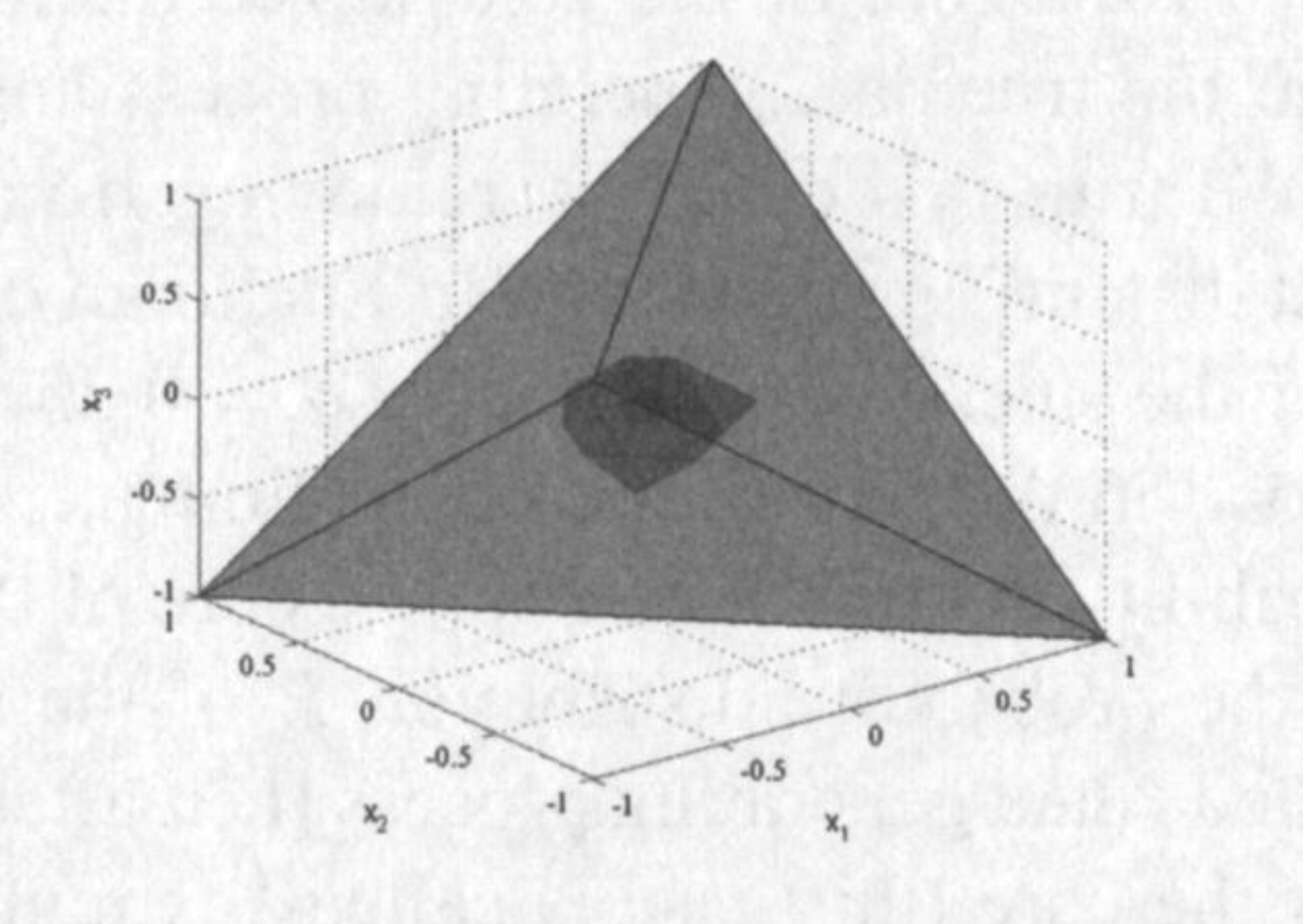
(c) $\theta=0.25$, Central DGP, $n=1000$, $90\%$ confidence

(d) $\theta=0.25$, Central DGP, $n=1000$, $95\%$ confidence

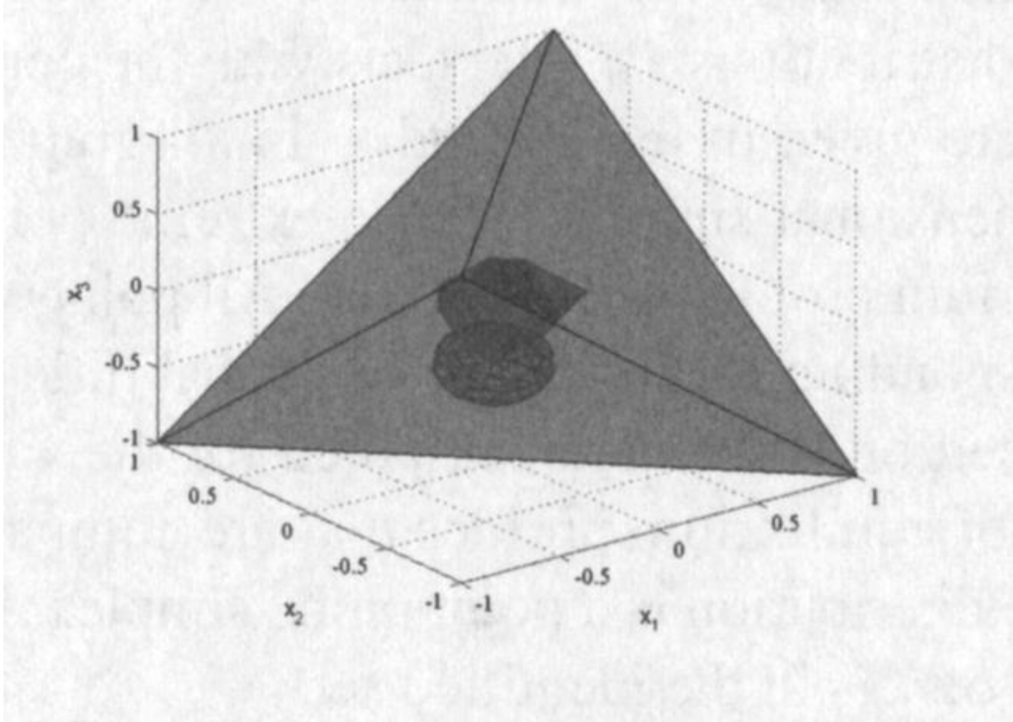
(e) $\theta=0.25$, Intermediate DGP, $n=100$, $90\%$ confidence

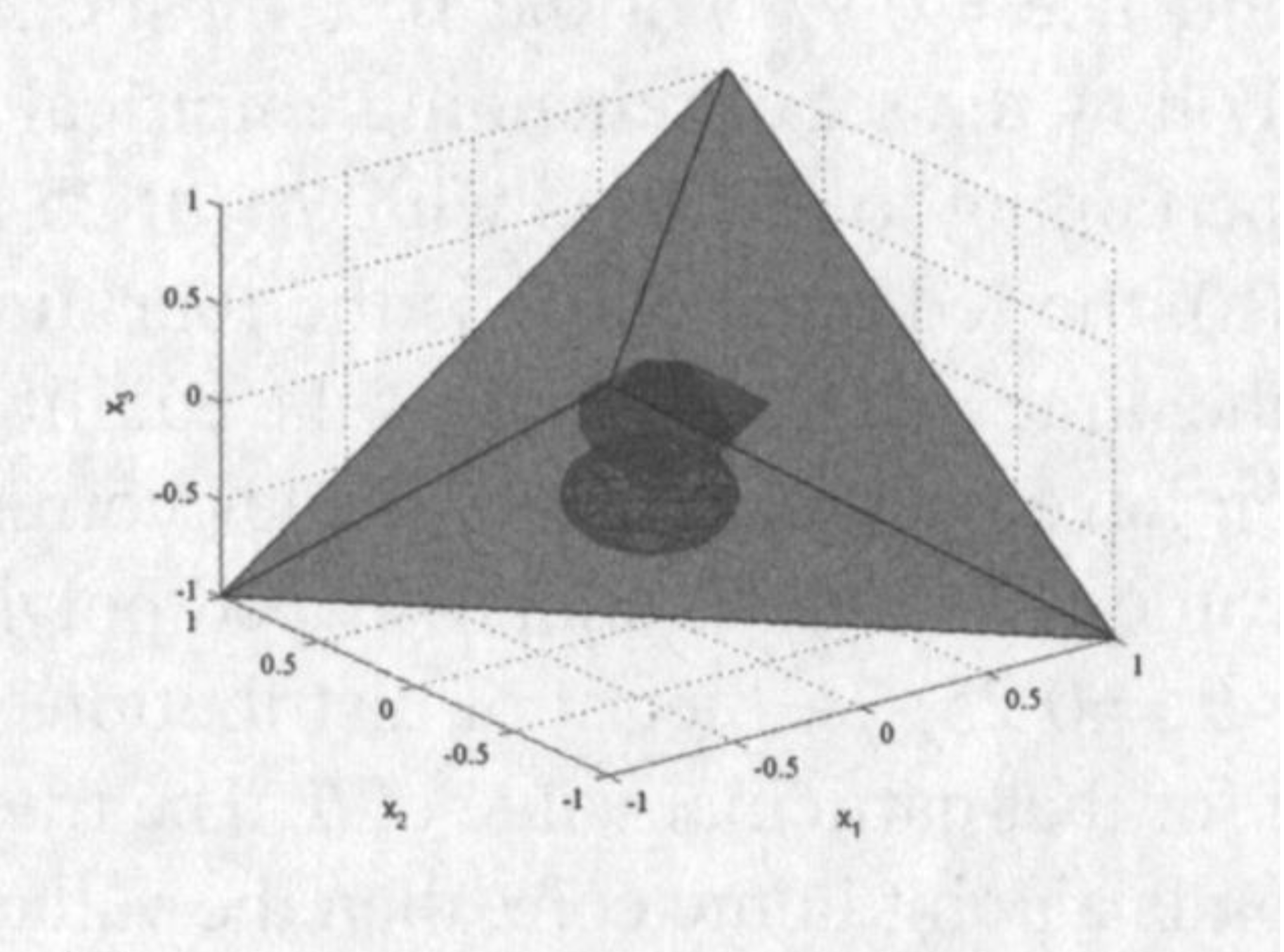
(f) $\theta=0.25$, Intermediate DGP, $n=100$, $95\%$ confidence

(g) $\theta=0.25$, Intermediate DGP, $n=1000$, $90\%$ confidence

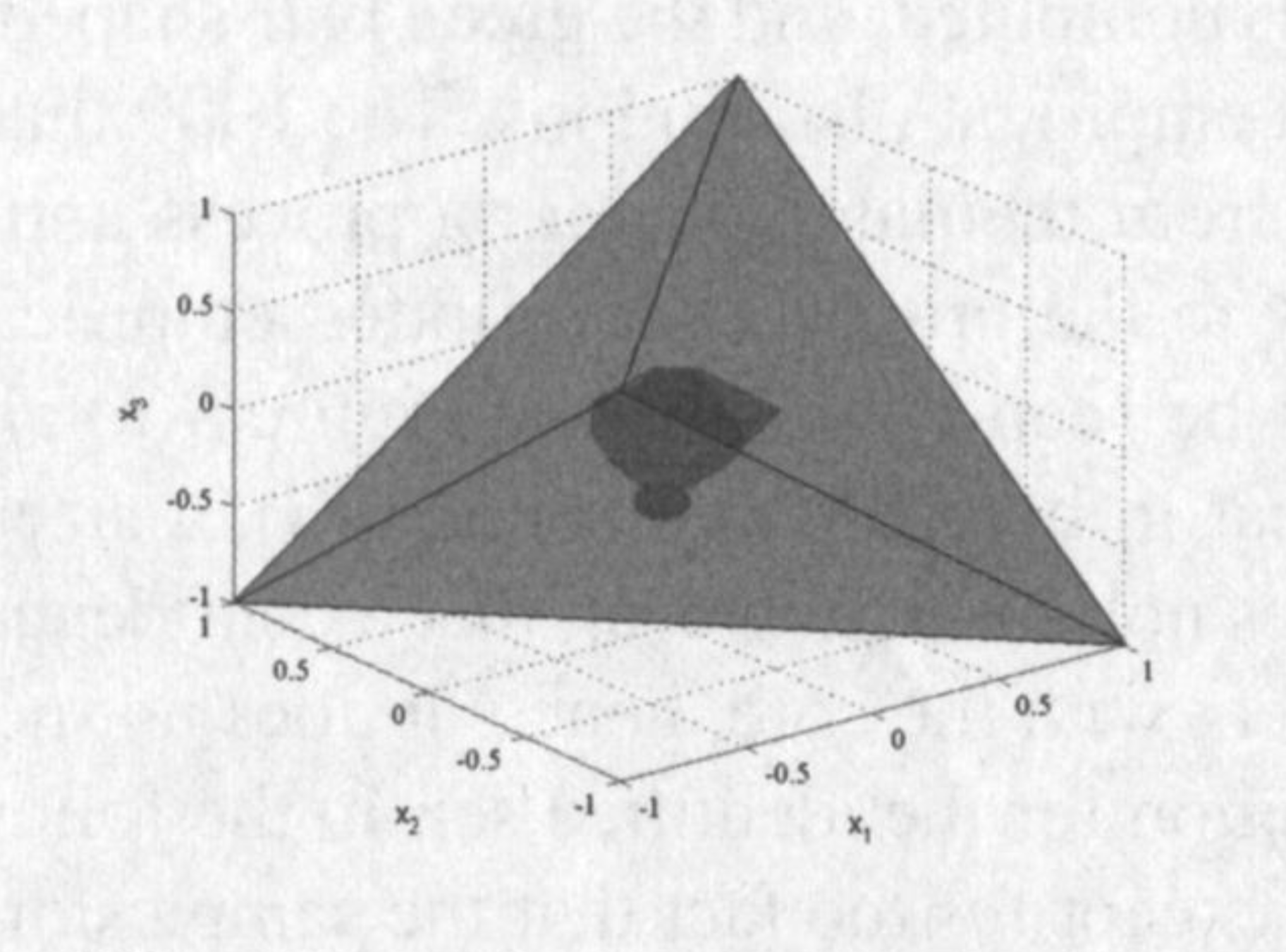
(h) $\theta=0.25$, Intermediate DGP, $n=1000$, $95\%$ confidence

Figure 9.

In figure 9(a), the core is plotted for the case $\theta=0.25$ and $10,000$ data series of size $n=100$ are drawn from the analytical center of the core. For each simulated sample, the empirical distribution is computed, and the green ball-shaped polyhedron is the set of $9,000$ out of the $10,000$ computed empirical distributions. The $1,000$ that are excluded are the most distant (in Euclidian distance) from the data generating process, and they are excluded for visual convenience. The sensitivity to the proportion of plotted empirical distributions (called “confidence” in the captions) can be seen by comparing figures 9(a) and 9(b), in which only $500$ outliers are excluded. We see that in both figures 9(a) and 9(b), a sizeable proportion of draws falls outside the core, which does not mean, however, that a confidence ball around such empirical distributions would not intersect with the core, hence it does not necessarily lead to the exclusion of $\theta$ from a confidence region for the identified set. In the following graphics, figures 9(c) and 9(d), the setup is identical, except for the fact that the samples drawn have size $1,000$. In that case, it is clear that all drawn empirical distributions are well within the core, which would lead to include $\theta$ in any reasonably constructed confidence region for the identified set. The observations are similar for figures 9(e) to 9(h), where the data are generated from the mid-point between the analytical center and an extreme point of the core. As a result, a larger proportion of simulated draws falls outside the core when $n=100$, but again, all draws a well within the core for $n=1,000$, so that $\theta$ would always be contained in a reasonably constructed confidence region for the identified set. In figures 9(e) to 9(h), the data is generated from an extreme point of the core. In such a case, a point in the neighbourhood of the data generating process is more likely to fall outside the core than inside it. Hence, for all sample sizes, the proportion of empirical distributions that fall outside the core is relatively stable, and larger than the proportion that falls inside the core. However, for larger sample sizes, we see that simulated empirical distributions are more likely to be within a predetermined neighbourhood of the core, so that the value $\theta$ is less likely to be excluded from a confidence region for the identified set. The cases where $\theta=0.5$ and $\theta=0.75$ are very similar and we do not report them here.

5. Empirical illustration: determinants of long term care for elderly parents

The applicability of the methodology proposed is best illustrated on data pertaining to our example 1.2.2. We estimate the determinants of long term care option choices for elderly parents in American families. The data consists of a sample of 948 families with two children drawn from the National Long Term Care Survey, sponsored by the National Institute of Aging and conducted by the Duke University Center for Demographic Studies under Grant number U01-AG007198, [19]. Elderly people were interviewed in 1984 about their living and care arrangements. The survey questions include gender and age of the children, the distance between homes of parents and each of the children, the disability status of the elderly parent (where disability is referred to as problems with “Activities of Daily Living or Instrumental Activities of Daily Living (ADL)”) and the number of hours per week each of the children devote to the care of the elderly parent. The dependent variable is the care provision for the parent. The parent is asked to list children (either at home or away from home) and how much each provides help. If only one child is listed as providing significant help, that child is designated the primary care giver. If more than one child is listed, the one providing the most hours is designated the primary care giver. If no child is listed or if the parent lives in a nursing home, then the parent is designated as “living alone.”

The observable choice of care option is modeled as in [22] as the outcome of a family bargaining game. The payoff to family member $i$, $i=1,2$ is represented as the sum of three terms. The first term $V_{ij}$ represents the value to child $i$ of care option $j$, where $j>0$ means child $j$ becomes the primary care giver and $j=0$ means the parent remains alone or is moved to a nursing home. The matrix $V=(V_{ij})_{ij}$ is known to both children. We suppose it takes the form

$$V=\left(\begin{array}[]{lll}\hskip 5.0pt0\hskip 10.0pt&\beta_{0}+ADL\beta&\beta_{0}+ADL\beta\\ \hskip 5.0pt0\hskip 10.0pt&\beta_{0}+ADL\beta+D_{1}\psi+F\alpha&\beta_{0}+ADL\beta\\ \hskip 5.0pt0\hskip 10.0pt&\beta_{0}+ADL\beta&\beta_{0}+ADL\beta+D_{2}\psi\end{array}\right)$$

where $ADL$ is a dummy variable that takes the value 1 if the parent has problems with activities of daily living or instrumental activities of daily living, $D_{i}$ is the distance between parent and child $i$, $F=1$ if child $1$ (who is first-born) is female, and zero otherwise and $\theta=(\beta_{0},\beta,\psi,\alpha)^{\prime}$ is a four dimensional parameter vector, unknown to the analyst. The value a family attaches to the fact that a non disabled parent is taken care of by one of the children is measured by $\beta_{0}$, whereas for a disabled parent, it is $\beta_{0}+\beta$. $\psi$ measures the disutility to the caregiver of living more than an hour away from the parent, and $\alpha$ measures the incremental utility of taking care of the parent for the firstborn daughter, as compared with a firstborn son.

In the data, $85\%$ of interviewed parents have problems with activities of daily living. $70\%$ of parents live alone. $46\%$ of first-born children are female, whereas $56\%$ of first-born who are primary care-takers are female. The female first-born effect was identified in [22], and we wish to see whether it is robust to our analysis that takes multiple equilibria in the game seriously.

Both children simultaneously decide whether or not to take part in the long term care decision. Suppose $M$ is the set of children who participate. The option chosen is option $j$ which maximizes the sum $\sum_{i\in M}V_{ij}$ among the available options (only participating children can become primary care givers). It is assumed that participants abide with the decision and that benefits are then shared equally among children participating in the decision through a monetary transfer $s_{i}$, which is the second term in the children’s payoff. The third term $\epsilon_{i}$ in the payoff is a random benefit from participation, which is $0$ for children who decide not to participate and distributed according to $\nu(.|\theta)$ for children who participate. All children observe the realizations of $\epsilon$, whereas the analyst only knows its distribution (the negative shock on participation is calibrated with a normal distribution $N(-3,1)$ for $\epsilon$. An alternative would have been a negative exponential distribution for $\epsilon$).

The payoff matrix of the participation game can be determined in the following way.

• If both children decide to participate, child i’s payoff (for $i=1,2$) is

  $$X_{i}=\max\left(0,\beta_{0}+ADL\beta+\frac{1}{2}(D_{1}\psi+F\alpha),\beta_{0}+ADL\beta+\frac{1}{2}D_{2}\psi\right)+\epsilon_{i}.$$

• If neither child participates, their payoffs are 0.

• If only child $1$ participates, child $1$’s payoff is

  $$X_{1}=\max\left(0,\beta_{0}+ADL\beta+D_{1}\psi+F\alpha\right)+\epsilon_{1}$$

  and child $2$’s payoff is

  $$X_{2}=\left(\beta_{0}+ADL\beta\right)1_{\{\beta_{0}+ADL\beta+D_{1}\psi+F\alpha\geq 0\}}.$$

• If only child $2$ participates, child $2$’s payoff is

  $$X_{2}=\max\left(0,\beta_{0}+ADL\beta+D_{2}\psi\right)+\epsilon_{2}$$

  and child $1$’s payoff is

  $$X_{1}=\left(\beta_{0}+ADL\beta\right)1_{\{\beta_{0}+ADL\beta+D_{2}\psi\geq 0\}}.$$

We do not observe participation, but only the chosen care option. To each equilibrium strategy profile corresponds a (almost surely) unique care option choice, hence for each participation shock $\epsilon$, we can derive the $G(\epsilon|F,D,ADL;\theta)$ as the set of probability measures on the set of care options $\{0,1,2\}$ induced by mixed strategy profiles, which are probabilities on the set of participation profiles $\{(N,N),(N,P),(P,N),(P,P)\}$. The Gambit software is a good option for the computation of $G(\epsilon|F,D,ADL;\theta)$.

The methodology proposed in the paper allows the construction of the identified set based on the hypothetical knowledge of the true distribution of the data. In order to account for sampling uncertainty, we appeal to the bootstrap procedure proposed in [28] to construct confidence regions for the identified set in such situations. The method relies on a bootstrap determination of a set function $A\mapsto\underline{P}(A|F,D,ADL)$ which is dominated by $P(A|F,D,ADL)$ (uniformly over $A\subseteq\{0,1,2\}$, $X$, $D$ and $ADL$) with probability $1-\alpha$ (the chosen level of significance, here $0.95$). Once $\underline{P}$ is determined, one proceeds as recommended in section 4.2. That is to say, we keep in the identified set only values of $\theta$ such that for all observed values of the explanatory variables, the minimum over $A\subseteq\{0,1,2\}$ of the function $\mathcal{L}(A|F,D,ADL;\theta)-\underline{P}(A|F,D,ADL;\theta)$ is non negative. The search over the 4-dimensional parameter space is conducted in the following way. First one finds a value of the parameter which lies within the confidence region (for instance the corresponding estimates in the analysis of [22] which achieves identification by removing multiplicity of equilibria), then one chooses a coarse discretization of $[-\pi,\pi]^{3}$ to search in all directions for the frontier point of the confidence region, which is assumed to be arc-connected (on each arc, we use a dichotomic search). The resulting frontier points are the extreme points of the confidence polytope. Each value of the parameter can be tested in a fraction of a second on a standard laptop, and the region can be constructed in a few hours, again on a standard laptop without parallel processing. The confidence region is a four dimensional polytope and 3, 2 or 1-dimensional confidence regions for subsets or linear combinations of parameters can be easily visualized as cuts from the confidence region using the matlab multiparametric MPT toolbox.

The variables chosen were those that were significant in [22]. We test the significance of each of the individual parameters by checking whether the hyperplanes defined by $\beta_{0}=0$, $\beta=0$, $\psi=0$ and $\alpha=0$ intersect with our $95\%$ confidence region. The range of values of $\beta_{0}$ is $\beta_{0}\in[-4.297,1.426]$. Hence, the hyperplane $\beta_{0}=0$ has non empty intersection with the confidence region, which means we fail to reject (at the $5\%$ level) the null hypothesis that the family values identically the fact that a non disabled parent lives alone or is taken care of by a family member. On the other hand, the range of values for $\beta$ is $\beta\in[1.976,7.297]$, so the half space $\beta\leq 0$ has empty intersection with the confidence region, and we reject the null hypothesis that a parent’s disability does not increase the value of care provided by the family. We also reject the hypothesis that distance between parent and caretaker is insignificant, as the range for $\psi$ is $\psi\in[-2.981,-1.306]$. Finally, we reject the hypothesis that gender of the firstborn child does not affect the chosen care option, as the range for $\alpha$ is $\alpha\in[0.409,2.405]$. Indeed, our results are still consistent with [22] in the finding that families value care provided by a firstborn daughter more than care provided by a firstborn son. Since the hypothesis that $\beta_{0}=0$ is not rejected, we slice the confidence region at $\beta_{0}=0$ to obtain the constrained confidence region, which is three dimensional and is represented (from four different angles) in figure 10. In the constrained region, the ranges for the three remaining parameters are considerably tighter, as $\beta\in[2.717,4.062]$, $\psi\in[-2.867,-1.365]$ and $\alpha\in[0.532,2.290]$. Two dimensional regions are also given for $(\alpha,\psi)$, when $\beta=3$, for $(\beta,\psi)$ when $\alpha=2$ and $(\beta,\alpha)$ when $\psi=-2$. These regions are plotted in figure 11. Notice the thin diagonal shapes of the regions, which makes them rather informative, as for instance simultaneous large values of $\psi$ and $\alpha$ are rejected, which roughly means that firstborn daughters living close by are not the only possible caregivers. Similarly, $\beta$ and $\psi$ are not simultaneously very large, so that either the disability effect is very large or the distance effect is very large, but not both.

(a)

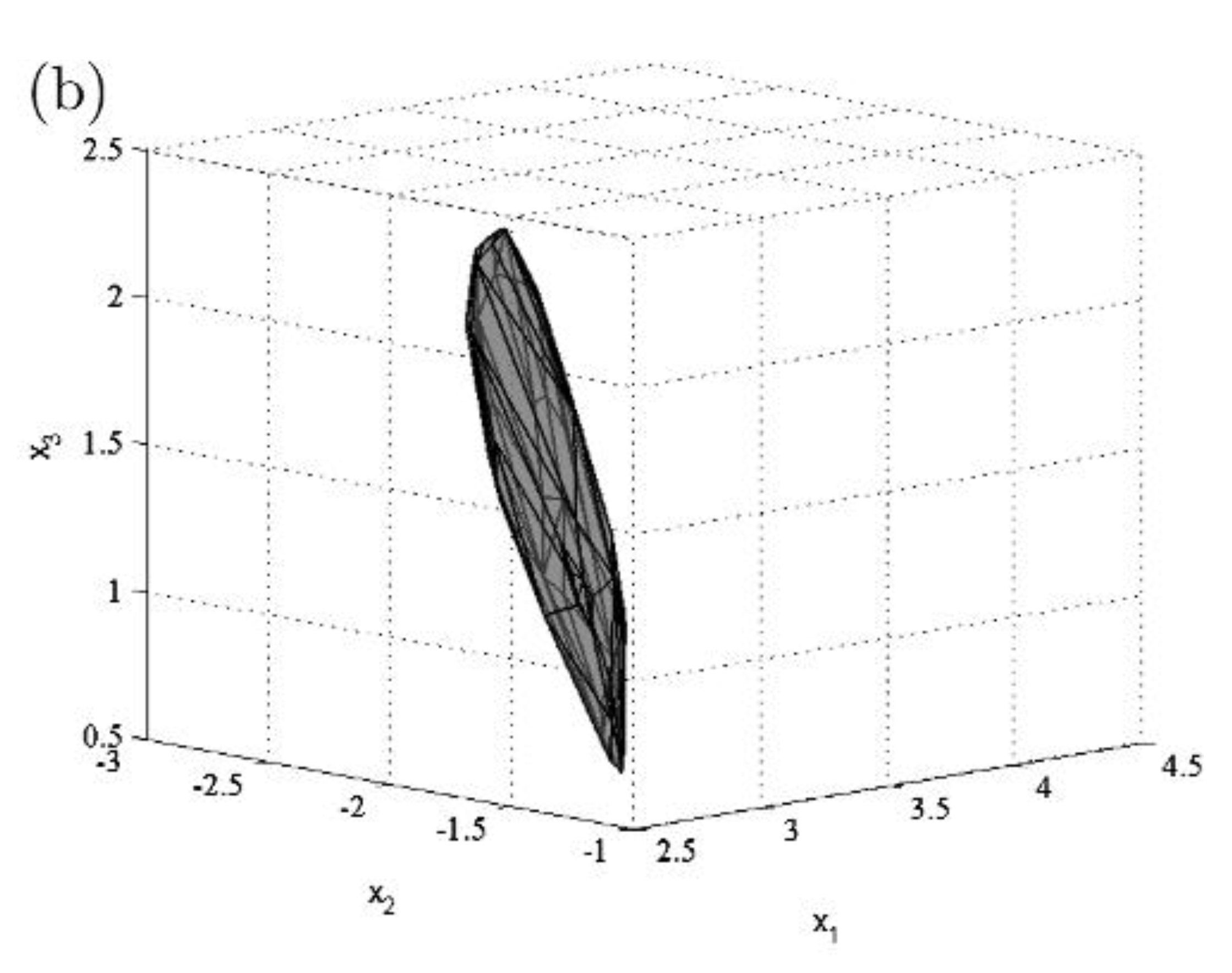
(b)

(c)

(d)

Figure 10. $(\beta,\psi,\alpha)$ region at $\beta_{0}=0$.

(a) $(\psi,\alpha)$ region at $(\beta_{0},\beta)=(0,3)$.

(b) $(\beta,\psi)$ region at $(\beta_{0},\alpha)=(0,2)$.

Figure 11. Bivariate confidence regions

Conclusion

In the context of models with multiple equilibria in pure and mixed strategies, we have proposed an equivalence result between the existence of an equilibrium selection mechanism compatible with the data and a finite set of inequalities characterizing the core of the model likelihood, and provided methods to reduce this number of inequalities to be checked with an appeal to the notion of core determining families and to efficient easily implementable combinatorial methods. The issue of statistical inference on the identified feature thus characterized is taken up in [27] and [25], which complement the seminal work of [15].

Appendix A Proofs of results in the main text

A.1. Proof of theorem 1

It suffices to show that for all $\theta\in\Theta$, statement 1 and statement 2 are equivalent, where statement 1 and statement 2 are defined as the following. Statement 1: $P(A|X)\leq\nu(\epsilon:\;G(\epsilon|X;\theta)\cap A\neq\varnothing|X;\theta)$ for all $A$ measurable subset of $\mathcal{Y}$, $X$-almost surely. Statement 2: For almost all $\epsilon$, there exists a probability measure $\pi(.|\epsilon,X)$ with support $G(\epsilon|X;\theta)$ such that $P(A|X)=\int_{\mathcal{U}}\pi(A|X;\theta)\nu(d\epsilon|X;\theta)$ for all $A$ measurable subset of $\mathcal{Y}$, $X$-almost surely. We proceed in six steps. Step 1: Since $G(\epsilon|X;\theta)$ is nonempty and closed by assumption, the set $\Delta(G(\epsilon|X;\theta))$ of probability measures on $\mathcal{Y}$ with support $G(\epsilon|X;\theta)$ is convex and closed in the topology of convergence in distribution. Step 2: Since $G(.|X;\theta)$ is a measurable correspondence, for any $f\in\mathcal{C}_{b}(\mathcal{Y})$, the set of all continuous and bounded real functions on $\mathcal{Y}$, the map $\epsilon\mapsto\sup\{\int fd\mu:\mu\in\Delta(G(\epsilon|X;\theta))\}$ is measurable. Step 3: By step 1 and step 2, we can apply theorem 3 of [47] to conclude that statement 2 is equivalent to $\int_{\mathcal{Y}}f(y)P(dy)\leq\int_{\mathcal{U}}\sup\{\int fd\mu:\mu\in\Delta(G(\epsilon|X;\theta))\}\nu(d\epsilon|X;\theta)$ for all $f\in\mathcal{C}_{b}(\mathcal{Y})$. Step 4: For any bounded continuous function $f$, we have $\sup\{\int fd\mu:\mu\in\Delta(G(\epsilon|X;\theta))\}=\max\{f(y):y\in G(\epsilon|X;\theta)\}$. Step 5: Call $\rho$ the Choquet capacity defined for all measurable subset $A$ of $\mathcal{Y}$ by $\rho(A)=\nu(\epsilon:\;G(\epsilon|X;\theta)\cap A\neq\varnothing|X;\theta)=\nu(G^{-1}(A|X;\theta)|X;\theta)$. We show that $\int_{\mathcal{U}}\max\{f(y):y\in G(\epsilon|X;\theta)\}\nu(d\epsilon|X;\theta)=\int_{\mathrm{Choquet}}fd\rho$, where the latter is the Choquet integral with respect to the Choquet capacity functional $\rho$, which is defined by $\int_{\mathrm{Choquet}}fd\rho=\int_{0}^{\infty}\rho(\{f\geq v\})\,\mbox{d}v+\int_{-\infty}^{0}\,(\rho(\{f\geq v\})-1)\,\mbox{d}v$. The latter can be rewritten $\int_{0}^{\infty}\nu\bigl{(}\epsilon:\;G(\epsilon|X;\theta)\cap\left\{f\geq v\right\}\neq\varnothing|X;\theta\bigr{)}\,\mbox{d}v+\int_{-\infty}^{0}\,(\nu\bigl{(}\epsilon:\;G(\epsilon|X;\theta)\cap\left\{f\geq v\right\}\neq\varnothing|X;\theta\bigr{)}-1)\,\mbox{d}v$, which is equal to $\int_{0}^{\infty}\nu\bigl{(}\epsilon:\;\max_{y\in G(\epsilon|X;\theta)}f(y)\geq v|X;\theta\bigr{)}\,\mbox{d}v+\int_{-\infty}^{0}\,(\nu\bigl{(}\epsilon:\;\max_{y\in G(\epsilon|X;\theta)}f(y)\geq v|X;\theta\bigr{)}-1)\,\mbox{d}v=\int_{\mathcal{U}}\max\{f(y):y\in G(\epsilon|X;\theta)\}\nu(d\epsilon|X;\theta)$, as we set out to show. Step 6: Finally, by monotone continuity, we have that $\int_{\mathcal{Y}}f(y)P(dy|X)\leq\int_{\mathrm{Choquet}}fd\rho$ for all $f\in\mathcal{C}_{b}(\mathcal{Y})$ is equivalent to the fact that $P(.|X)$ is in the core of the Choquet capacity functional $\rho$, which is statement 1.

A.2. Proof of proposition 3

We first state a general criterion for the core determining property.

Proposition 3.

A class $\mathcal{A}(\theta)$ of subsets of $\mathcal{Y}$ is core determining for the Choquet capacity $A\mapsto\mathcal{L}(A|X;\theta)=\nu(\epsilon:\;G(\epsilon|X;\theta)\cap A\neq\varnothing|X;\theta)$ if for every measurable subset $A$ of $\mathcal{Y}$, there exists nonnegative integers $K,L,N$, $\alpha_{k}$, $k=1,\ldots,K$, and elements $A_{1},\ldots,A_{K}$ of $\mathcal{A}(\theta)$ such that for almost all $y\in\mathcal{Y}$ and almost all $\epsilon\in\mathcal{U}$,

$$1_{A}(y)\leq\frac{1}{N}\left(\sum_{k=1}^{K}\alpha_{k}1_{A_{k}}(y)-L\right)\hskip 10.0pt\mathrm{and}\hskip 10.0pt1_{\{G(\epsilon|X;\theta)\cap A\neq\varnothing\}}(\epsilon)\geq\frac{1}{N}\left(\sum_{k=1}^{K}\alpha_{k}1_{\{G(\epsilon|X;\theta)\cap A_{k}\neq\varnothing\}}(\epsilon)-L\right).$$ (A.1)

Proof of proposition 3.

Subtracting the second inequality in equation A.1 yields:

$$1_{A}-1_{\{\epsilon:\,G(\epsilon|X;\theta)\cap A\neq\varnothing\}}\leq\frac{1}{N}\left(\sum_{k=1}^{K}\alpha_{k}(1_{A_{k}}-1_{\{\epsilon:\,G(\epsilon|X;\theta)\cap A_{k}\neq\varnothing\}})\right)$$

Taking expectations (conditionally on $X$) on both sides of the previous equation yields

$$P(A|X)-\nu(\epsilon:\;G(\epsilon|X;\theta)\cap A\neq\varnothing|X;\theta)\leq\frac{1}{N}\left(\sum_{k=1}^{K}\alpha_{k}(P(A_{k}|X)-\nu(\epsilon:\;G(\epsilon|X;\theta)\cap A_{k}\neq\varnothing|X;\theta))\right).$$

This in turn implies that $P(A|X)\leq\nu(\epsilon:\;G(\epsilon|X;\theta)\cap A\neq\varnothing|X;\theta)$ if $P(A_{k}|X)\leq\nu(\epsilon:\;G(\epsilon|X;\theta)\cap A_{k}\neq\varnothing|X;\theta)$ for each $k$, which means that $\mathcal{A}(\theta)$ is indeed core determining, which completes the proof.∎

We now turn to the proof of theorem 4. We consider the equivalent problem where the set of latent variables $\mathcal{U}$ is replaced by the set of predicted combinations of equilibria $\mathcal{U}^{\ast}$. We keep the same notation for the equilibrium correspondence $G$, and call $u$ the elements of $\mathcal{U}^{\ast}$. For simplicity, we also drop the dependence on $X$ and $\theta$ in the notation, so that $G:u\mapsto G(u)$ is a correspondence between $\mathcal{U}^{\ast}$ and $\mathcal{Y}$. Note that by construction $G(u)=u\in 2^{\mathcal{Y}}$, but it is not the identity when considered as a correspondence. Let $A$ be a subset of $\mathcal{Y}$. Call $K_{y}$ the cardinality of $\mathcal{Y}$ and $K_{u}$ the cardinality of $\mathcal{U}^{\ast}$. List all elements of $\mathcal{Y}$ as $y_{k}$, $k=1\ldots,K_{y}$ and all elements of $\mathcal{U}^{\ast}$ as $u_{k}$, $k=1,\ldots,K_{u}$. For any $u\in\mathcal{U}^{\ast}$, define $k_{u}$ by $u=u_{k_{u}}$ and for any $y\in\mathcal{Y}$, define $k_{y}$ by $y=y_{k_{y}}$. As usual, denote $G^{-1}(A)$ the set $\{u\in\mathcal{U}^{\ast}:G(u)\cap A\neq\varnothing\}$. Call $\Delta 1_{G^{-1}(A)}(u_{1})=1_{G^{-1}(A)}(u_{1})$ and for $k\geq 2$, $\Delta 1_{G^{-1}(A)}(u_{k})=1_{G^{-1}(A)}(u_{k})-1_{G^{-1}(A)}(u_{k-1})$. Call $\Delta 1^{+}_{G^{-1}(A)}$ and $\Delta 1^{-}_{G^{-1}(A)}$ the positive and negative parts of $\Delta 1_{G^{-1}(A)}$. By construction, we have for any $u\in\mathcal{U}^{\ast}$,

$$1_{G^{-1}(A)}(u) = \sum_{k=1}^{k_{u}}\Delta 1_{G^{-1}(A)}(u_{k})$$

$$= \sum_{k=1}^{K_{u}}1_{\{u_{k},\ldots,u_{K_{u}}\}}(u)\Delta 1_{G^{-1}(A)}(u_{k})$$

$$= \sum_{k=1}^{K_{u}}1_{\{u_{k},\ldots,u_{K_{u}}\}}(u)\Delta 1^{+}_{G^{-1}(A)}(u_{k})-\sum_{k=1}^{K_{u}}1_{\{u_{k},\ldots,u_{K_{u}}\}}(u)\Delta 1^{-}_{G^{-1}(A)}(u_{k})$$

$$= \sum_{k=1}^{K_{u}}1_{\{u_{k},\ldots,u_{K_{u}}\}}(u)\Delta 1^{+}_{G^{-1}(A)}(u_{k})+\sum_{k=1}^{K_{u}}1_{\{u_{1},\ldots,u_{k-1}\}}(u)\Delta 1^{-}_{G^{-1}(A)}(u_{k})-\sum_{k=1}^{K_{u}}\Delta 1^{-}_{G^{-1}(A)}(u_{k}).$$

We then apply proposition 3 with the following choice of parameters. $K=2K_{u}$, $\alpha_{j}/N=\Delta 1^{+}_{G^{-1}(A)}(u_{j})$, $j=1\ldots,K_{u}$, $\alpha_{j}/N=\Delta 1^{-}_{G^{-1}(A)}(u_{j-K_{u}})$, $j=K_{u}+1,\ldots,2K_{u}$, and $L/N=\sum_{k=1}^{K_{u}}\Delta 1^{-}_{G^{-1}(A)}(u_{k})$. There remains to show that

$$1_{A}(y)\leq\sum_{k=1}^{K_{u}}1_{\{\inf G(u_{k}),\ldots,y_{K_{y}}\}}(y)\Delta 1^{+}_{G^{-1}(A)}(u_{k})+\sum_{k=1}^{K_{u}}1_{\{y_{1},\ldots,\sup G(u_{k-1})\}}(y)\Delta 1^{-}_{G^{-1}(A)}(u_{k})-\sum_{k=1}^{K_{u}}\Delta 1^{-}_{G^{-1}(A)}(u_{k})$$

to complete the proof. The latter follows from

$$\sum_{k=1}^{K_{u}}1_{\{\inf G(u_{k}),\ldots,y_{K_{y}}\}}(y)\Delta 1^{+}_{G^{-1}(A)}(u_{k})+\sum_{k=1}^{K_{u}}1_{\{y_{1},\ldots,\sup G(u_{k-1})\}}(y)\Delta 1^{-}_{G^{-1}(A)}(u_{k})-\sum_{k=1}^{K_{u}}\Delta 1^{-}_{G^{-1}(A)}(u_{k})$$ (A.2)

$$= \sum_{k=1}^{K_{u}}1_{\{\inf G(u_{k}),\ldots,y_{K_{y}}\}}(y)\Delta 1^{+}_{G^{-1}(A)}(u_{k})-\sum_{k=1}^{K_{u}}1_{\{y_{k_{\sup G(u_{k-1})}+1},\ldots,y_{K_{u}}\}}(y)\Delta 1^{-}_{G^{-1}(A)}(u_{k}).$$

We have $k_{\inf G(u_{k})}<k_{\sup G(u_{k-1})}+1$ (otherwise, there would be a $y$ that belongs to none of the $u$’s, i.e. that is never an equilibrium outcome, and it could be eliminated from the analysis). Hence (A.2) is equal to

$$\sum_{k=1}^{K_{u}}1_{\{\inf G(u_{k}),\ldots,y_{k_{\sup G(u_{k-1})}+1}\}}(y)\Delta 1^{+}_{G^{-1}(A)}(u_{k})$$

$$\hskip 100.0pt+\sum_{k=1}^{K_{u}}1_{\{y_{k_{\sup G(u_{k-1})}+1},\ldots,y_{K_{u}}\}}(y)(\Delta 1^{+}_{G^{-1}(A)}(u_{k})-\Delta 1^{-}_{G^{-1}(A)}(u_{k}))$$

$$= \sum_{k=1}^{K_{u}}1_{\{\inf G(u_{k}),\ldots,y_{k_{\sup G(u_{k-1})}+1}\}}(y)\Delta 1^{+}_{G^{-1}(A)}(u_{k})+\sum_{k=1}^{K_{u}}1_{\{y_{k_{\sup G(u_{k-1})}+1},\ldots,y_{K_{u}}\}}(y)\Delta 1_{G^{-1}(A)}(u_{k})$$

$$\geq \sum_{k=1}^{K_{u}}1_{\{\inf G(u_{k}),\ldots,y_{k_{\sup G(u_{k-1})}+1}\}}(y)\Delta 1_{G^{-1}(A)}(u_{k})+\sum_{k=1}^{K_{u}}1_{\{y_{k_{\sup G(u_{k-1})}+1},\ldots,y_{K_{u}}\}}(y)\Delta 1_{G^{-1}(A)}(u_{k})$$

$$= \sum_{k=1}^{K_{u}}1_{\{\inf G(u_{k}),\ldots,y_{K_{u}}\}}(y)\Delta 1_{G^{-1}(A)}(u_{k})=1_{A}(y),$$

Which completes the proof.

A.3. Proof of Theorem 3

First note that any specification of the latent variable $\epsilon$ that produces the same combinations of equilibria listed in $\mathcal{U}^{\ast}$ with the same probabilities are observationally equivalent. We can therefore replace $\mathcal{U}$ by $\mathcal{U}^{\ast}$, where each $u\in\mathcal{U}^{\ast}$ has probability $Q(u|X;\theta)=\nu(\epsilon:\;G(\epsilon|X;\theta)=u|X;\theta)$, and redefine $G$ as the correspondence from $\mathcal{U}^{\ast}$ to $\mathcal{Y}$ defined by $G(u)=u$. By theorem 1, $\theta$ belongs to the identified set if and only if for any subset $A$ of $\mathcal{Y}$, $P(A|X)\leq\nu(\epsilon:\;G(\epsilon|X;\theta)\cap A\neq\varnothing|X;\theta)$ or equivalently $P(A|X)\leq Q(G^{-1}(A)|X;\theta)$. By proposition 1 of [27], this is equivalent to the existence of a probability $\pi$ on $\mathcal{Y}\times\mathcal{U}^{\ast}$ with marginal distributions $P(.|X)$ and $Q(.|X;\theta)$ and such that $\pi\{(y,u)\in\mathcal{Y}\times\mathcal{U}^{\ast}:y\in u\}=1$, in other words such that it is supported on the subset of pairs $(y,u)$ such that $y\in u$. This completes the proof.

A.4. Proof of Proposition 2

The term in parenthesis in (4.1) is a convex combination of elements of $G(\epsilon|X;\theta)$, hence the existence of an equilibrium mechanism with the required property is equivalent to the existence of a family $\Pi(.,\epsilon|X;\theta)$ of probability measures on $\mathcal{Y}$ such that $\Pi(.,\epsilon|X;\theta)\in\mathrm{co}(G(\epsilon|X;\theta))$, $\epsilon$-almost surely. By Choquet’s Theorem (see [16]), this implies that for any function $f$ on $\mathcal{Y}$,

$$\sum_{\mathcal{Y}}f(y)\Pi(y,\epsilon|X;\theta)\leq\max\left\{\sum_{\mathcal{Y}}f(y)s(y);s\in G(\epsilon|X;\theta)\right\},$$

which, by integration over $\epsilon$, implies

$$\sum_{\mathcal{Y}}f(y)\mathbb{P}(Y=y|X)\leq\int\left\{\max_{s\in G(\epsilon|X;\theta)}\sum_{\mathcal{Y}}f(y)s(y)\right\}d\nu(\epsilon|X).$$

The latter yields the desired representation after dividing both sides by the norm of $f$.

Conversely, suppose that for all functions $f$ on $\mathcal{Y}$, we have

$$\sum_{\mathcal{Y}}f(y)\mathbb{P}(y|X)\leq\int L_{\epsilon|X;\theta}(f)d\nu(\epsilon|X;\theta),$$

where

$$L_{\epsilon|X;\theta}(f)=\max\left\{\sum_{\mathcal{Y}}f(y)s(y);s\in G(\epsilon|X;\theta)\right\}.$$

By the Strassen Disintegration Theorem (see [47]), there exists a map $\epsilon\mapsto\Pi(.,\epsilon|X;\theta)$ such that for all $y\in\mathcal{Y}$, $\mathbb{P}(Y=y|X)=\int\Pi(y,\epsilon|X;\theta)d\nu(\epsilon|X)$ and $\Pi(.,\epsilon|X;\theta)\leq L_{\epsilon|X;\theta}(.)$, $\epsilon$-almost surely. Again by the Choquet Theorem, the latter condition is equivalent to $\Pi(.,\epsilon|X;\theta)\in\mathrm{co}(G(\epsilon|X;\theta))$, $\epsilon$-almost surely, and the result follows.

A.5. Proof of Lemma 2

Consider a game with equilibrium correspondence $G$ and call $\mu$ the upper envelope of the equilibrium correspondence, i.e. for all $A\subset\mathcal{Y}$, $\mu(A)=\sup_{\sigma\in G}\sigma(A)$. Let $Core(\mu)$ be the core of $\mu$ (probabilities set-wise dominated by $\mu$) and for a given subset $A$ of $\mathcal{Y}$, call $C_{A}$ the set of probabilities in $Core(\mu)$ that attain the supremum at $A$, i.e. such that $P(A)=\mu(A)$. Section 3.1 of [46] shows that the game has a regular core if and only if for each $P\in Core(\mu)$, the class of subsets $\{A\subset\mathcal{Y}\}$ such that $P\in C_{A}$ is closed under union and intersection. Consider a pure strategy equilibrium in $G$, denoted $\delta_{y}$. Then $\delta_{y}\in C_{A}$ if and only if $y\in A$, and the class of sets that contains $y$ is closed under unions and intersections. Consider now the unique proper mixed strategy equilibrium $\sigma$ in $G$. Then, $\sigma\in C_{A}$ is and only if $A$ does not meet the domain of any pure strategy equilibrium in $G$, a property which is also preserved under unions and intersections. The result follows.

A.6. Proof of Theorem 5

By proposition 2 , the identified set is characterized as the set of parameter values $\theta$ such that for all functions $f$ on $\mathcal{Y}$, $E_{P}(f(Y)|X)\leq\int\left(\max_{\sigma\in G(\epsilon|X;\theta)}E_{\sigma}(f(Y))\right)d\nu(\epsilon|X;\theta)$. By [45], the functional

$$\tilde{\mathcal{L}}:f\mapsto\int\left(\max_{\sigma\in G(\epsilon|X;\theta)}E_{\sigma}(f(Y))\right)d\nu(\epsilon|X;\theta)$$

is the Choquet integral associated with the Choquet capacity $\mathcal{L}:B\mapsto\mathcal{L}(B|X;\theta)=\tilde{\mathcal{L}}(1_{B}|X;\theta)$, because the latter is submodular, as a mixture of submodular capacities, and (dropping the dependence on $X$ and $\theta$ from notation) the Choquet integral satisfies the following two properties:

• Monotonicity: If $f(y)\leq t(y)$ for all $y\in\mathcal{Y}$, then $\tilde{\mathcal{L}}(f)\leq\tilde{\mathcal{L}}(t)$,

• Comonotonic additivity: If $f$ and $t$ are comonotonic, i.e. if $(f(y_{1})-f(y_{2}))(t(y_{1})-t(y_{2}))\geq 0$ for all $y_{1},y_{2}\in\mathcal{Y}$, then $\tilde{\mathcal{L}}(f+t)=\tilde{\mathcal{L}}(f)+\tilde{\mathcal{L}}(t)$.

Note that submodularity of $\mathcal{L}:B\mapsto\mathcal{L}(B)=\tilde{\mathcal{L}}(1_{B})$ (i.e. $\mathcal{L}(A\cap B)+\mathcal{L}(A\cup B)\leq\mathcal{L}(A)+\mathcal{L}(B)$ for all $A,B\subseteq\mathcal{Y}$) is equivalent to convexity of the Choquet integral $\tilde{\mathcal{L}}$ (see proposition 3 of [45] or theorem 6.13 page 212 of [24]). By definition of the Choquet integral, $\tilde{\mathcal{L}}$ can be written

$$\tilde{\mathcal{L}}(f)=\int_{0}^{\infty}\mathcal{L}(f\geq x)dx+\int_{-\infty}^{0}(\mathcal{L}(f\geq x)-1)dx.$$

Whenever a probability $P$ on $\mathcal{Y}$ satisfies $P(B)\leq\mathcal{L}(B)$ for all $B\in\subseteq\mathcal{Y}$, it follows that

$$E_{P}(f(Y)) = \sum_{y\in\mathcal{Y}}f(y)P(y)$$

$$= \int_{0}^{\infty}P(f\geq x)dx+\int_{-\infty}^{0}(P(f\geq x)-1)dx$$

$$\leq \int_{0}^{\infty}\mathcal{L}(f\geq x)dx+\int_{-\infty}^{0}(\mathcal{L}(f\geq x)-1)dx$$

$$= \tilde{\mathcal{L}}(f).$$

The converse is immediately seen by taking the indicator functions for $f$, and the result follows.

Appendix B Complements

B.1. Likelihood in the example 1.2.2

• $\mathcal{L}(\{(0,1)\}|\theta)=\nu(\epsilon_{1}<\theta,\epsilon_{2}>-2\theta)$

• $\mathcal{L}(\{(1,0)\}|\theta)=\nu(\epsilon_{2}<\theta,\epsilon_{1}>-2\theta)$

• $\mathcal{L}(\{(0,1),(1,0)\}|\theta)=1-\nu(\epsilon_{1}<-2\theta,\epsilon_{2}<-2\theta)-\nu(\epsilon_{1}>\theta,\epsilon_{2}>\theta)$

• $\mathcal{L}(\{(0,1),(1,0),(1,1)\}|\theta)=1-\nu(\epsilon_{1}<-2\theta,\epsilon_{2}<-2\theta)$

• $\mathcal{L}(\{(0,1),(1,0),(0,0)\}|\theta)=1-\nu(\epsilon_{1}>\theta,\epsilon_{2}>\theta)$

• $\mathcal{L}(\{(0,0)\}|\theta)=\mathbb{E}_{\nu}[(\theta-\epsilon_{2})(\theta-\epsilon_{1})/(9\theta^{2})1{\{\epsilon\in[-2\theta,\theta]^{2}\}}]+\nu(\epsilon_{1}<-2\theta,\epsilon_{2}<-2\theta)$

• $\mathcal{L}(\{(1,1)\}|\theta)=\mathbb{E}_{\nu}[(2\theta+\epsilon_{2})(2\theta+\epsilon_{1})/(9\theta^{2})1{\{\epsilon\in[-2\theta,\theta]^{2}\}}]+\nu(\epsilon_{1}>\theta,\epsilon_{2}>\theta)$

• $\mathcal{L}(\{(1,1),(0,0)\}|\theta)=\mathcal{L}(\{(1,1)\}|\theta)+\mathcal{L}(\{(0,0)\}|\theta)$.

• $\mathcal{L}(\{(0,0),(0,1)\}|\theta)=\mathcal{L}(\{(0,1)\}|\theta)+\nu(\epsilon_{1}<-2\theta,\epsilon_{2}<-2\theta)$

• $\mathcal{L}(\{(0,0),(1,0)\}|\theta)=\mathcal{L}(\{(1,0)\}|\theta)+\nu(\epsilon_{1}<-2\theta,\epsilon_{2}<-2\theta)$

• $\mathcal{L}(\{(1,1),(0,1)\}|\theta)=\mathcal{L}(\{(0,1)\}|\theta)+\nu(\epsilon_{1}>\theta,\epsilon_{2}>\theta)$

• $\mathcal{L}(\{(1,1),(1,0)\}|\theta)=\mathcal{L}(\{(1,0)\}|\theta)+\nu(\epsilon_{1}>\theta,\epsilon_{2}>\theta)$

• $\mathcal{L}(\{(1,1),(0,0),(0,1)\}|\theta)=\mathcal{L}(\{(0,1)\}|\theta)+\nu(\epsilon_{1}>\theta,\epsilon_{2}>\theta)+\nu(\epsilon_{1}<-2\theta,\epsilon_{2}<-2\theta)$

• $\mathcal{L}(\{(1,1),(0,0),(1,0)\}|\theta)=\mathcal{L}(\{(1,0)\}|\theta)+\nu(\epsilon_{1}>\theta,\epsilon_{2}>\theta)+\nu(\epsilon_{1}<-2\theta,\epsilon_{2}<-2\theta)$

References

- [1] D. Ackerberg, L. Benkard, S. Berry and A. Pakes “Econometric tools for analyzing market outcomes” Handbook of Econometrics, Volume 6A, 2007
- [2] Donald Andrews, Steven Berry and Panle Jia “Placing bounds on parameters of entry games in the presence of multiple equilibria” unpublished manuscript, 2003
- [3] Donald Andrews and Gustavo Soares “Inference for Parameters Defined by Moment Inequalities Using Generalized Moment Selection” unpublished manuscript, 2007
- [4] Zvi Artstein “Distributions of random sets and random selections” In Israel Journal of Mathematics 46, 1983
- [5] Patrick Bajari, Han Hong and Stephen P. Ryan “Identification and Estimation of a Discrete Game of Complete Information” In Econometrica 78.5, 2010, pp. 1529–1568 eprint: https://onlinelibrary.wiley.com/doi/pdf/10.3982/ECTA5434
- [6] Ari Beresteanu and Francesca Molinari “Asymptotic properties for a class of partially identified models” forthcoming in Econometrica, 2007
- [7] Arie Beresteanu, Ilya Molchanov and Francesca Molinari “Sharp Identification Regions in Models with Convex Predictions: Games, Individual Choice, and Incomplete Data” In Centre for Microdata Methods and Practice, Institute for Fiscal Studies, CeMMAP working papers 79, 2009
- [8] Steve Berry “Estimation of a model of entry in the airline industry” In Econometrica 60, 1992, pp. 889–917
- [9] Steve Berry and Elie Tamer “Identification in models of oligopoly entry” In Advances in Economics and Econometrics Cambridge University Press, 2006, pp. 46–85
- [10] Alberto Bisin, Andrea Moro and Giorgio Topa “Empirical Content of Models with Multiple Equilibria” In unpublished manuscript, 2002
- [11] Paul Bjorn and Quang Vuong “Simultaneous Equations Models for Dummy Endogenous Variables: A Game Theoretic Formulation with an Application to Labor Force Participation”, 1984
- [12] Tim Bresnahan and P. Reiss “Entry in monopoly markets” In Review of Economic Studies 57, 1990, pp. 531–553
- [13] William A. Brock and Steven N. Durlauf “Discrete Choice with Social Interactions” In The Review of Economic Studies 68.2 [Oxford University Press, Review of Economic Studies, Ltd.], 2001, pp. 235–260
- [14] Ivan Canay “EL Inference for Partially Identified Models: Large Deviation Optimality and Bootstrap Validity” unpublished manuscript, 2007
- [15] Victor Chernozhukov, Han Hong and Elie Tamer “Estimation and Confidence Regions for Parameter Sets in Econometric Models” In Econometrica 75, 2007, pp. 1243–1285
- [16] Gustave Choquet “Theory of capacities” In Annales de l’Institut Fourier 5, 1954, pp. 131–295
- [17] Federico Ciliberto and Elie Tamer “Market structure and multiple equilibria in airline markets” unpublished manuscript, 2006
- [18] John Dagsvik and Boyan Jovanovic “Was the Great Depression a low-level equilibrium?” In European Economic Review 38.9, 1994, pp. 1711–1729
- [19] Duke “National Long Term Care Survey” In Public use data set produced and distributed by the Duke University Center for Demographic Studies with funding from the National Institute on Aging under Grant No. U01-AG007198, 1999
- [20] Federico Echenique “Mixed equilibria in games of strategic complementarities” In Economic Theory 22, 2003, pp. 33–44
- [21] Ivar Ekeland, Alfred Galichon and Marc Henry “Optimal Transportation and the Falsifiability of Incompletely Specified Economic Models” In Economic Theory 42.2 Springer, 2010, pp. 355–374
- [22] Maxim Engers and Steven Stern “Family Bargaining and Long Term Care” In International Economic Review 43, 2002, pp. 73–114
- [23] L. Ford and D. Fulkerson “A simple algorithm for finding maximal network flows and an application to the Hitchcock problem” In Canadian Journal of Mathematics 9, 1957, pp. 210–218
- [24] Satoru Fujishige “Submodular Functions and Optimization” Amsterdam, The Netherlands: Elsevier, 2005
- [25] Alfred Galichon and Marc Henry “Dilation Bootstrap. A methodology for constructing confidence regions with partially identified models” unpublished manuscript, 2006
- [26] Alfred Galichon and Marc Henry “Inference in incomplete models” Columbia University Discussion Paper 0506-28 available at http://www.columbia.edu/cu/economics/discpapr/DP0506-28.pdf, 2006
- [27] Alfred Galichon and Marc Henry “A test of non-identifying restrictions and confidence regions for partially identified parameters” unpublished manuscript, 2007
- [28] Alfred Galichon and Marc Henry “Set Identification in Models with Multiple Equilibria” In The Review of Economic Studies 78, 2011, pp. 1264–1298
- [29] D. Gillies “Some theorems on n-person games” Princeton Ph.D., 1953
- [30] C Gourieroux, J J Laffont and A Monfort “Coherency Conditions in Simultaneous Linear Equation Models with Endogenous Switching Regimes” In Econometrica 48.3, 1980, pp. 675–695
- [31] James Heckman “Dummy endogenous variables in a simultaneous equations system” In Econometrica 46, 1978, pp. 931–960
- [32] James Heckman, Jeffrey Smith and Nancy Clements “Making the most out of programme evaluation and social experiments: accounting for heterogeneity in programme impacts” In Review of Economic Studies 64, 1997, pp. 487–535
- [33] Guido Imbens and Charles Manski “Confidence intervals for partially identified parameters” In Econometrica 72, 2004, pp. 1845–1859
- [34] Boyan Jovanovic “Observable implications of models with multiple equilibria” In Econometrica 57, 1989, pp. 1431–1437
- [35] Tjallin Koopmans “Optimum utilization of the transportation system” In Econometrica 17, 1949, pp. 136–146
- [36] Tjallin Koopmans and O. Reiersol “The identification of structural characteristics” In Annals of Mathematical Statistics 21, 1950, pp. 165–181
- [37] Charles Manski “Nonparametric bounds on treatment effects” In American Economic Review 80, 1990, pp. 319–323
- [38] Charles Manski and Elie Tamer “Inference on Regressions with Interval Data on a Regressor or Outcome” In Econometrica 70, 2002, pp. 519–546
- [39] Paul Milgrom and John Roberts “Rationalizability, Learning, and Equilibrium in Games with Strategic Complementarities” In Econometrica 58.6 [Wiley, Econometric Society], 1990, pp. 1255–1277
- [40] Hervé Moulin “Cooperative Microeconomics” Princeton: Princeton University Press, 1995
- [41] Ariel Pakes, Jack Porter, Kate Ho and Joy Ishii “Moment inequalities and their application” unpublished manuscript, 2004
- [42] Christos Papadimitriou and Kenneth Steiglitz “Combinatorial Optimization: Algorithms and Complexity” Dover, 1998
- [43] Joe Romano and Azeem Shaikh “Inference for identifiable parameters in partially identified econometric models” forthcoming in the Journal of Statistical Planning and Inference, 2006
- [44] Adam Rosen “Confidence sets for partially identified parameters that satisfy a finite number of moment inequalities” unpublished manuscript, 2006
- [45] David Schmeidler “Integral representation without additivity” In Proceedings of the American Mathematical Society 97, 1986, pp. 255–261
- [46] Lloyd S. Shapley “Cores of convex games” In International Journal of Game Theory 1.1, 1971, pp. 11–26
- [47] Victor Strassen “The existence of probability measures with given marginals” In Journal of Mathematical Statistics 36, 1965, pp. 423–439
- [48] Andrew Sweeting “Coordination Games, Multiple Equilibria and the Timing of Radio Commercials”, 2005
- [49] Elie Tamer “Incomplete simultaneous discrete response model with multiple equilibria” In Review of Economic Studies 70, 2003, pp. 147–165
- [50] Donald M. Topkis “Supermodularity and Complementarity” Princeton: Princeton University Press, 1998
- [51] Xavier Vives “Nash equilibrium with strategic complementarities” In Journal of Mathematical Economics 19.3, 1990, pp. 305–321