Upper bounds on the one-arm exponent for
dependent percolation models

Abstract.

We prove upper bounds on the one-arm exponent $\eta_{1}$ for a class of dependent percolation models which generalise Bernoulli percolation; while our main interest is level set percolation of Gaussian fields, the arguments apply to other models in the Bernoulli percolation universality class, including Poisson-Voronoi and Poisson-Boolean percolation. More precisely, in dimension $d=2$ we prove that $\eta_{1}\leq 1/3$ for continuous Gaussian fields with rapid correlation decay (e.g. the Bargmann-Fock field), and in $d\geq 3$ we prove $\eta_{1}\leq d/3$ for finite-range fields, both discrete and continuous, and $\eta_{1}\leq d-2$ for fields with rapid correlation decay. Although these results are classical for Bernoulli percolation (indeed they are best-known in general), existing proofs do not extend to dependent percolation models, and we develop a new approach based on exploration and relative entropy arguments. The proof also makes use of a new Russo-type inequality for Gaussian fields, which we apply to prove the sharpness of the phase transition and the mean-field bound for finite-range fields.

1. Introduction

The critical phase of percolation models is believed to be described by a set of critical exponents which govern the power-law behaviour of macroscopic observables at, or near, criticality. These exponents have been thoroughly investigated for Bernoulli percolation (see, e.g., [28, Chapter 9]) and there is a general expectation that, by universality, they are identical within the class of dependent percolation models with sufficient decay of correlations. However not much is rigorously known about critical exponents for dependent percolation models.

In this paper we study the one-arm exponent governing the distribution of critical clusters with large diameter. Using a new approach we establish upper bounds on the exponent for a wide class of dependent percolation models induced by the excursion sets of Gaussian fields (‘Gaussian percolation’), which contains Bernoulli site percolation as a special case; roughly-speaking our results extend the state-of-the-art for Bernoulli percolation to this general class.

Although we focus on Gaussian percolation, our approach could be adapted to other models in the same universality class, including Poisson-Voronoi and Poisson-Boolean percolation.

1.1. Gaussian percolation and the one-arm exponent

We consider the following class of dependent percolation models defined on either $\mathbb{R}^{d}$ or $\mathbb{Z}^{d}$, $d\geq 2$. Let $f$ be either (i) a continuous stationary-ergodic centred Gaussian field on $\mathbb{R}^{d}$, or (ii) a stationary-ergodic centred Gaussian field on $\mathbb{Z}^{d}$. We write $\mathbb{X}\in\{\mathbb{R},\mathbb{Z}\}$ depending on the domain $\mathbb{X}^{d}$ of the field.

For $\ell\in\mathbb{R}$ write $\mathbb{P}_{\ell}[\cdot]$ to denote the law of $f+\ell$ (abbreviating $\mathbb{P}=\mathbb{P}_{0}$). Then the excursion sets $\{f+\ell\geq 0\}:=\{x\in\mathbb{X}^{d}:f(x)+\ell\geq 0\}$ induce a stationary-ergodic percolation model on $\mathbb{X}^{d}$ via the connectivity relation

$$\{A\longleftrightarrow B\}:=\{\text{there exists a path in $\mathbb{X}^{d}$ in $\{f\geq 0\}$ that intersects $A$ and $B$}\}$$

for closed sets $A,B\subset\mathbb{X}^{d}$. When $f$ is an i.i.d. field on $\mathbb{Z}^{d}$, this model is equivalent to Bernoulli site percolation on $\mathbb{Z}^{d}$. When $f$ is a continuous field on $\mathbb{R}^{d}$, $d=2$, the model is self-dual at $\ell=0$, and in that sense is similar to bond percolation on $\mathbb{Z}^{2}$.

Let $\Lambda_{R}:=[-R,R]^{d}\cap\mathbb{X}^{d}$. By monotonicity we may define the critical level $\ell_{c}=\ell_{c}(f)\in[-\infty,\infty]$ of the model to be the unique level satisfying

$$\theta(\ell):=\mathbb{P}_{\ell}[\Lambda_{1}\longleftrightarrow\infty]:=\lim_{R\to\infty}\mathbb{P}_{\ell}[\Lambda_{1}\longleftrightarrow\partial\Lambda_{R}]=\begin{cases}0&\text{if }\ell<\ell_{c},\\ >0&\text{if }\ell>\ell_{c}.\end{cases}$$

By self-duality one expects that $\ell_{c}=0$ if $f$ is continuous and $d=2$, whereas in general one expects $\ell_{c}\in(-\infty,\infty)$ (see [49, 43, 26, 47, 42] and [40, 41] respectively for sufficient conditions, which are implied by Assumption 1.1 below). It is believed that $\theta(\ell_{c})=0$, although so far this is only known if $d=2$ and $f$ is positively-correlated [32, 24, 4], or if $f$ is i.i.d. and $d\geq 11$ [23].

For Bernoulli percolation [12, 2], as well as certain other (non-Gaussian) dependent percolation models [19, 18, 20], it is known that $\theta(\ell)$ satisfies the mean-field bound

(MFB) $$\theta(\ell)\geq c(\ell-\ell_{c})$$

for a constant $c=c(d)$ and $\ell>\ell_{c}$ sufficiently close to $\ell_{c}$; this bound is expected to be tight for dimensions $d\geq d_{c}=6$ in which critical exponents take their mean-field value. We expect (MFB) to be true in general for Gaussian percolation but this has not yet been established; in this paper we prove it for Gaussian models with finite-range dependence.

At criticality $\ell=\ell_{c}$ it is believed that connection probabilities obey a power law, in the sense that there exists a one-arm exponent $\eta_{1}>0$ such that, as $R\to\infty$ and for $r=o(R)$,

(1.1) $$\mathbb{P}_{\ell_{c}}[\Lambda_{r}\longleftrightarrow\partial\Lambda_{R}]=(r/R)^{\eta_{1}+o(1)}.$$

While the existence of $\eta_{1}$ is not known (except in the i.i.d. case in high dimension), since we are interested in upper bounds we define

(1.2) $$\eta_{1}:=\liminf_{R\to\infty}\frac{-\log\mathbb{P}_{\ell_{c}}[\Lambda_{1}\longleftrightarrow\partial\Lambda_{R}]}{\log R}.$$

Clearly upper bounds on (1.2) imply upper bounds on the exponent in (1.1) assuming its existence. Note however that the choice of $\liminf$, rather than $\limsup$, in the definition of $\eta_{1}$ is deliberate and yields an a priori weaker bound (c.f. Remark 1.5).

For Bernoulli percolation it is expected that

$$\eta_{1}=\begin{cases}&\!\!\!\!5/48\qquad\ \ \hskip 1.42271ptd=2,\qquad\qquad 0.48\ldots\qquad d=3,\qquad\qquad 0.95\ldots\qquad d=4,\\ &\!\!\!\!1.5\ldots\qquad d=5,\qquad\qquad 2\qquad\qquad\hskip 8.5359ptd\geq d_{c}=6.\end{cases}$$

According to the Harris criterion (see [57], or [8] for further discussion), the value of $\eta_{1}$ should be the same for all Gaussian models whose correlations decay faster than $|x|^{-2/\nu}$ as $x\to\infty$, where $\nu=\nu(d)>0$ is the correlation length exponent of Bernoulli percolation (see Section 1.3 for a definition). For models with stronger correlations, the value of $\eta_{1}$ may be different [57, 15].

1.2. Upper bounds on the one-arm exponent

Recall that $f$ is a stationary-ergodic centred Gaussian field on the state space $\mathbb{X}^{d}$, $d\geq 2$, where $\mathbb{X}\in\{\mathbb{R},\mathbb{Z}\}$. We refer to $\mathbb{X}=\mathbb{R}$ and $d=2$ as the self-dual case.

We will always assume that $f$ has a spatial moving average representation $f=q\star W$, where $q\in L^{2}(\mathbb{X}^{d})\neq 0$ is Hermitian (i.e. $q(x)=q(-x)$), $W$ is the white noise on $\mathbb{X}^{d}$ (interpreted as a collection of i.i.d. standard Gaussian random variables indexed by $\mathbb{Z}^{d}$ if $\mathbb{X}=\mathbb{Z}$), and $\star$ denotes convolution. Such a representation always exists if the covariance kernel $K(\cdot):=\mathbb{E}[f(0)f(\cdot)]=(q\star q)(\cdot)$ is absolutely integrable, since then we may define $q:=\mathcal{F}[\sqrt{\rho}]$, where $\mathcal{F}$ denotes the Fourier transform and $\rho=\mathcal{F}[K]$ is the spectral density of the field. Bernoulli site percolation corresponds to the case $\mathbb{X}=\mathbb{Z}$ and $q(x)=\mathds{1}_{x=0}$.

We will further assume that $q$ satisfies the following basic properties:

Assumption 1.1 (Basic assumptions).

 

1. (Decay of correlations, with parameter $\beta>d$) There exists a $c>0$ such that, for all $x\in\mathbb{R}^{d}$,

   (1.3) $$|q(x)|\leq c|x|^{-\beta}.$$

2. (Symmetry) $q$ is symmetric under negation and permutation of the coordinate axes.

3. (Regularity, only if $\mathbb{X}=\mathbb{R}$) $q\in C^{3}(\mathbb{R}^{d})$, all derivatives up to third-order are in $L^{2}(\mathbb{R}^{d})$, and (1.3) holds with $|\nabla q(x)|$ in place of $|q(x)|$.

Let us make some remarks on Assumption 1.1. The decay condition ensures that $K=q\star q\in L^{1}(\mathbb{X}^{d})$, and so correlations decay polynomially with exponent $\beta>d$. This also ensures that the spectral density $\rho=\mathcal{F}[K]$ is continuous. The symmetry assumption is crucial for our results in self-dual case (for instance to prove RSW estimates), but it also simplifies some aspects of the proof in general. In the case $\mathbb{X}=\mathbb{R}$, the regularity condition ensures that $f$ is $C^{2}$-smooth almost surely. Along with the continuity of the spectral measure, this also implies that $(f,\nabla f,\nabla^{2}f)$ is non-degenerate (i.e. its evaluation on a finite number of distinct points is a non-degenerate Gaussian vector, see [6, Lemma A.2]). Finally, as we mentioned above, Assumption 1.1 is sufficient to prove that $\ell_{c}\in(-\infty,\infty)$ [40, 41], and that $\ell_{c}=0$ in the self-dual case (see [42, Theorem 1.3] and Remark 1.9 therein).

For most of our results we also assume that

(POS) $$\int q:=\int_{\mathbb{X}^{d}}q(x)\,dx>0,$$

where for a function $g:\mathbb{Z}^{d}\to\mathbb{R}$ we interpret $\int_{D}g(x)\,dx$ as $\sum_{x\in D\cap\mathbb{Z}^{d}}g(x)$. This is equivalent to the spectral density $\rho$ being strictly positive at the origin, and is a natural assumption when studying how properties of a Gaussian field change with the level; see e.g. [43, 7].

For some of our results we further assume that $f$ is positively correlated:

(PA) $$K(x)=(q\star q)(x)\geq 0 x\in\mathbb{X}^{d}$$ for all .

This is equivalent to the FKG inequality holding for the field (i.e. the field is positively associated), so that events increasing with respect to the field are positively correlated [46]. Note that (PA) is stronger than (POS), since the former implies that $\rho=\mathcal{F}[K]$ is positive definite, and so strictly positive at the origin.

We are now ready to state our results. Our first result concerns Gaussian percolation with finite-range of dependence:

Theorem 1.2 (Finite-range models).

Suppose $f$ satisfies Assumption 1.1, (POS), and $q$ has bounded support. Then $\eta_{1}\leq d/3$. In the self-dual case ($f$ is continuous and $d=2$), if additionally (PA) holds, then there exists $c>0$ such that, for all $R\geq 1$,

$$\mathbb{P}_{p_{c}}[\Lambda_{1}\longleftrightarrow\partial\Lambda_{R}]\geq cR^{-1/3},$$

and in particular $\eta_{1}\leq 1/3$.

Remark 1.3.

Except in some very special cases, the bounds in Theorem 1.2 match the best-known bounds for Bernoulli percolation:

1. For Bernoulli percolation on $\mathbb{Z}^{d}$ in general dimension $d\geq 3$, the best known bound is $\eta_{1}\leq d/3$ [10], deduced by combining the hyperscaling inequality $\eta_{1}\leq d/(1+\delta)$, where $\delta$ is the critical exponent governing the volume of critical clusters, with the mean-field bound $\delta\geq 2$ [2]. In sufficiently high dimension $d\geq 11$, it is known that $\eta_{1}$ takes its mean-field value $\eta_{1}=2$ [36, 23], see also Corollary 1.3 below. Note that the bound $\eta_{1}\leq d/3$ is expected to be tight in dimension $d_{c}=6$ (indeed, it implies that the upper critical dimension $d_{c}$ is at least $6$ since it shows that $\eta_{1}<2$ for $d\leq 5$).

2. For general self-dual Bernoulli models in dimension $d=2$, the best-known bound is $\eta_{1}\leq 1/3$ [34] Sharper results are known for two very specific models, namely $\eta_{1}\leq 1/6$ for bond percolation on $\mathbb{Z}^{2}$ [17], and the exact value $\eta_{1}=5/48$ for site percolation on the triangular lattice [53].

Previously for Gaussian percolation it was only known that $\eta_{1}\leq d-1$ and $\eta_{1}\leq 1/2$ in the self-dual case; the latter is a consequence of RSW estimates [5, 48, 43], and see [13] for the former.

Remark 1.4.

We emphasise that the bound $\eta_{1}\leq d/3$ in Theorem 1.2 does not assume positive correlations, and so applies to a class of models that lack positive associations.

Remark 1.5.

Unlike in the self-dual case, our proof that $\eta_{1}\leq d/3$ does not allow us to deduce the pointwise lower bound

$$\mathbb{P}_{\ell_{c}}[\Lambda_{1}\longleftrightarrow\partial\Lambda_{R}]\geq cR^{-d/3},$$

since we establish $\eta_{1}\leq d/3$ by obtaining a contradiction with $\mathbb{P}_{\ell_{c}}[\Lambda_{1}\longleftrightarrow\partial\Lambda_{R}]\leq cR^{-d/3-\varepsilon}$. This is also true for the previous argument establishing $\eta_{1}\leq d/3$ for Bernoulli percolation [10, 2].

Remark 1.6.

In the self-dual case we also obtain a bound on the ‘one-arm exponent’ for level lines, namely that there exists a $c>0$ such that, for all $R\geq 1$,

(1.4) $$\mathbb{P}_{\ell_{c}}\big{[}\{\text{there exists a path in $\{f=0\}$ that intersects $\Lambda_{1}$ and $\partial\Lambda_{R}$}\}\big{]}\geq cR^{-2/3}.$$

To deduce $\eta_{1}\leq 1/3$ we use the observation that, by the FKG inequality and self-duality, the left-hand side of (1.4) is bounded above by the square of $\mathbb{P}_{\ell_{c}}[\Lambda_{1}\longleftrightarrow\partial\Lambda_{R}]$, see (3.1).

Remark 1.7.

Clearly if $q$ has bounded support then $f$ is finite-range dependent, but we do not know whether every finite-range $f$ can be represented as $q\star W$ for $q$ with bounded support (although this seems very natural). Certainly this is true assuming positive correlations or if $d=1$ [22]. It is also known [51] that if $f$ is finite-range and isotropic (i.e. its law is rotationally symmetric) then it can be represented as a countable sum of independent $f_{i}=q_{i}\star W_{i}$ for $q_{i}$ with uniformly bounded support. Since it is straightforward to extend our proof to handle such fields, the conclusion of Theorem 1.2 (and Theorem 1.16 below) are also true if we replace the assumption that $q$ has bounded support with the assumption that $f$ is finite-range dependent, and is either positively-correlated or isotropic.

Our next result extends Theorem 1.2 to a class of models with unbounded range of dependence. This depends on the decay exponent $\beta>d$ in Assumption 1.1, and recovers the bounds in Theorem 1.2 in the $\beta\to\infty$ limit.

Recall that the mean-field bound (MFB) is expected to hold in general for Gaussian percolation. In this paper we prove it only for finite-range models, see Theorem 1.16 below; for general models we instead introduce it as an assumption.

Theorem 1.8 (Models with polynomial correlation decay).

Suppose $f$ satisfies Assumption 1.1 with parameter $\beta>d$, and (POS).

1. If $d\geq 3$ and $\beta>4d-4$, then $\eta_{1}\leq\min\{\frac{d-2+\alpha(3d-1)}{1+2\alpha},d-1\}$ where $\alpha=\frac{3d-4}{2\beta-5d+4}$.

2. If $d\geq 2$, $\beta>2d-1$, and (MFB) holds, then $\eta_{1}\leq\min\{\max\{\frac{d}{3}+\frac{\alpha(d-1)}{3},\frac{\alpha(2d-1)}{3}\},d-1\}$ where $\alpha=\frac{3d-2}{2\beta-d}$.

3. If $f$ is continuous and $d=2$, $\beta>\frac{8}{3}$, and (PA) holds, then $\eta_{1}\leq\min\{\frac{1}{3}+\frac{5}{6(\beta-1)},\frac{1}{2}\}$.

Corollary 1.9 (Models with faster-than-polynomial correlation decay).

Suppose $f$ satisfies Assumption 1.1 for every parameter $\beta$.

1. If $d\geq 3$ then $\eta_{1}\leq d-2$.

2. If $d\geq 2$ and (MFB) holds, then $\eta_{1}\leq\frac{d}{3}$.

3. If $f$ is continuous and $d=2$, and if (PA) holds, then $\eta_{1}\leq 1/3$.

Proof.

Take $\beta\to\infty$ in Theorem 1.8. ∎

To illustrate Corollary 1.9 we consider two important fields to which it applies:

Example 1.10.

The Bargmann-Fock field is the continuous stationary Gaussian field on $\mathbb{R}^{d}$ with covariance kernel $K(x)=e^{-|x|^{2}/2}$ (see [5] for background and motivation). This field satisfies Assumption 1.1 for every parameter $\beta$ and also (PA), hence Corollary 1.9 applies, although it is not yet known whether (MFB) holds.

Example 1.11.

The massive Gaussian free field (MGFF) is the stationary Gaussian field on $\mathbb{Z}^{d}$ whose covariance kernel is the Green function of a simple random walk on $\mathbb{Z}^{d}$ killed at exponential rate $m>0$ (see [50] for a precise definition and motivation). We claim that the MGFF satisfies Assumption 1.1 for every parameter $\beta$. Indeed the spectral density of the MGFF is proportional to $\rho(s_{1},\ldots,s_{d})=(m+1-d^{-1}\sum_{i}\cos(s_{i})))^{-1}$, and since $\sqrt{\rho}$ is smooth with all derivatives absolutely integrable, $q=\mathcal{F}[\sqrt{\rho}]$ decays faster than any polynomial. Since also (PA) holds, Corollary 1.9 applies. Although it is not yet known that (MFB) holds, we believe that the approach in [19] can be adapted to prove this (see the comments in [16, Section 1.2]).

1.3. Relations to other critical exponents

Our methods also give bounds on $\eta_{1}$ in terms of other critical exponents, some of which appear to be new even for Bernoulli percolation.

For simplicity we state these results only in the case of Bernoulli site percolation, although similar results to Theorems 1.2 and 1.8 could be proven under more general assumptions. The proofs also go through unchanged for Bernoulli bond percolation. For the remainder of the subsection we assume that $\mathbb{X}=\mathbb{Z}$ and $q(x)=\mathds{1}_{x=0}$.

Let us introduce the relevant exponents. Recall the mean-field bound (MFB) on $\theta(\ell)$. It is expected that $\theta(\ell)\to 0$ as a power law as $\ell\downarrow\ell_{c}$; although this is not known rigorously (except in high dimension), we will assume that the corresponding exponent exists

$$\beta=\lim_{\ell\downarrow\ell_{c}}\frac{\log\theta(\ell)}{\log|\ell_{c}-\ell|}\in(0,\infty).$$

Below criticality $\ell<\ell_{c}$, it is known that connection probabilities decay exponentially [39, 2, 21] and that the limit

$$\frac{1}{\xi(\ell)}:=\lim_{R\to\infty}\frac{-\log\mathbb{P}_{\ell}[\Lambda_{1}\longleftrightarrow\partial\Lambda_{R}]}{R}\in(0,\infty)$$

exists [28, Theorem 6.10]. The correlation length $\xi(\ell)$ is expected to diverge as a power law as $\ell\uparrow\ell_{c}$, and we will again assume that the corresponding exponent exists

$$\nu=\lim_{\ell\uparrow\ell_{c}}\frac{-\log\xi(\ell)}{\log|\ell_{c}-\ell|}\in(0,\infty).$$

Similarly, as $\ell\uparrow\ell_{c}$ the susceptibility $\chi(\ell):=\sum_{v\in\mathbb{Z}^{d}}\mathbb{P}_{\ell}[0\longleftrightarrow v]<\infty$ is expected to diverge as a power law, and we will assume the existence of

$$\gamma=\lim_{\ell\uparrow\ell_{c}}\frac{-\log\chi(\ell)}{\log|\ell_{c}-\ell|}\in(0,\infty).$$

Finally we also assume that the critical two-point function decays as a power law with exponent

$$d-2+\eta:=\lim_{|v|_{\infty}\to\infty}\frac{-\log\mathbb{P}_{\ell_{c}}[0\longleftrightarrow v]}{\log|v|_{\infty}}\in(0,\infty),$$

where $|\cdot|_{\infty}$ denotes the sup-norm. We remark that $\beta\leq 1$ because of (MFB), and it is well known that $\nu\geq 2/d$ [11], $\gamma\geq 1$ [3], and $\eta\leq 1$ [29].

Theorem 1.12.

For Bernoulli percolation on $\mathbb{Z}^{d}$, assuming the existence of $\beta,\nu,\gamma$ and $\eta$,

(1.5) $$\frac{2-\gamma}{\nu}\leq\eta_{1}\leq\bar{\eta}_{1}\leq\min\Big{\{}d-\frac{2}{\nu},\frac{2-\eta}{2/\beta-1}\Big{\}}\leq 2-\eta,$$

where $\bar{\eta}_{1}$ is defined as in (1.2) with limsup replacing liminf. Moreover $\eta_{1}\leq\frac{d}{2/\beta+1}$.

Remark 1.13.

To our knowledge the bounds in (1.5) are new even for Bernoulli percolation, and $\eta_{1}\geq\frac{2-\gamma}{\nu}$ may be of particular interest as a lower bound on $\eta_{1}$. The bound $\eta_{1}\leq\frac{d}{2/\beta+1}$ is implied by the hyperscaling inequality in [10].

In sufficiently high dimension it is known that the exponents $\nu$, $\gamma$ and $\eta$ exist and take their mean-field values $\nu=1/2$ [30], $\gamma=1$ [3], and $\eta=0$ [31]. Hence Theorem 1.12 gives a new proof of the result of Kozma and Nachmias that $\eta_{1}=2$ in high dimension:

Corollary 1.14 ([36]).

For Bernoulli percolation on $\mathbb{Z}^{d}$, there exists $d_{0}>0$ such that, if $d\geq d_{0}$,

$$\lim_{R\to\infty}\frac{-\log\mathbb{P}_{\ell_{c}}[\Lambda_{1}\longleftrightarrow\partial\Lambda_{R}]}{\log R}=2.$$

Remark 1.15.

Our argument is significantly simpler than the one in [36], however it yields only

$$c_{1}R^{-2}\leq\mathbb{P}_{\ell_{c}}[\Lambda_{1}\longleftrightarrow\partial\Lambda_{R}]\leq c_{2}R^{-2}(\log R)^{4}$$

whereas [36] proved that $\mathbb{P}_{p_{c}}[\Lambda_{1}\longleftrightarrow\partial\Lambda_{R}]\asymp R^{-2}$ in the sense of bounded ratios (see Remark 3.5). Another difference is that we deduce $\eta_{1}=2$ in any dimension from the bounds $\nu\leq 1/2$ and $\eta\geq 0$ (see Remark 3.5, or recall the Fischer inequality $\gamma/\nu\leq 2-\eta$), whereas the argument in [36] uses as input $d>6$ and the two-sided bound $\eta=0$ (or more precisely $\mathbb{P}_{\ell_{c}}[0\longleftrightarrow v]\asymp|v|_{\infty}^{-d+2}$).

1.4. Sharpness of the phase transition for finite-range models

As part of the proof of Theorem 1.2 we establish the mean-field bound (MFB) for finite-range models. For this we adapt the approach of Duminil-Copin, Raoufi and Tassion [19]; as in [19] (and related contexts [2, 39]), this argument also yields the sharpness of the phase transition.

Theorem 1.16 (Sharpness of the phase transition for finite-range models).

Suppose $f$ satisfies Assumption 1.1 and $q$ has bounded support. Then the mean-field bound (MFB) holds. Moreover, for every $\ell<\ell_{c}$ there exist $c_{1},c_{2}>0$ such that, for $R\geq 1$,

(1.6) $$\mathbb{P}_{\ell}[\Lambda_{1}\longleftrightarrow\partial\Lambda_{R}]\leq c_{1}e^{-c_{2}R}.$$

Remark 1.17.

For Gaussian percolation, the exponential decay in (1.6) was only known so far in two cases: (i) in the self-dual case assuming positive correlations [43], and (ii) for certain positively-correlated Gaussian fields on $\mathbb{Z}^{d}$ [16, 27]. The mean-field bound (MFB) was not yet known for any Gaussian models.

We emphasise that in Theorem 1.16 we do not assume positive correlations, so this theorem holds for a class of models lacking positive associations. The proof also does not require the symmetry condition in Assumption 1.1.

1.5. Elements of the proof: the ‘entropic’ bound, and a new Russo-type inequality

The existing upper bounds on $\eta_{1}$ for Bernoulli percolation rely heavily on specific properties of this model (such as the BK inequality, or for the sharper results on specific lattices, also on properties of parafermionic observables) and do not extend easily to dependent percolation models. We develop a new approach based on exploration and relative entropy arguments.

There are two main ingredients in our approach, giving upper and lower bounds respectively on the change in probability of events as $\ell$ varies:

1. A non-differential ‘entropic’ upper bound, with control in terms of revealment probabilities of explorations.

2. A ‘Russo-type inequality’ giving a lower bound on the derivative for increasing events, which when combined with the OSSS inequality also gives control in terms of revealment probabilities of explorations.

In the self-dual case we compare these inequalities when applied to square-crossing events at criticality; by a judicious choice of algorithm the revealment probabilities are controlled by one-arm probabilities for level lines (c.f. Remark 1.6). In the general case we first use the Russo-type inequality to establish the mean-field bound (MFB), and then compare this to the entropic bound applied to arm events in the critical and slightly supercritical regimes.

Since we believe these ingredients to be of independent interest, we describe them in detail:

1.5.1. The entropic bound

For context, let us first state a well-known bound for Bernoulli percolation. Recall the concept of a randomised algorithm (or ‘decision tree’ or ‘exploration’ depending on the context):

Definition 1.18 (Randomised algorithms).

Let $X=(X_{i})_{i\in\mathbb{N}}$ be a countable set of random variables taking values in arbitrary measurable spaces, and let $Z=(Z_{i})_{i\in\mathbb{N}}$ be an auxiliary sequence of independent uniform random variables. A (randomised) algorithm $\mathcal{A}$ on $X$ is a random sequence $X^{\mathcal{A}}=(X_{\varphi(1)},..,X_{\varphi(i)},..)$ such that, for each $i\in\mathbb{N}$, $\varphi(i)\in\mathbb{N}$ is distinct from all $\varphi(j)$, $j<i$, and depends only on (i) $(X_{\varphi(1)},..,X_{\varphi(i-1)})$, and (ii) the auxiliary randomness $Z_{i}$. The sequence $X^{\mathcal{A}}$ can be either infinite or finite; in the latter case we say that $\mathcal{A}$ terminates, and a real number is returned which is a measurable function of $X^{\mathcal{A}}$. We say that $\mathcal{A}$ determines an event $A$ if it almost surely terminates and returns the value $\mathds{1}_{A}$. The revealment probability $\textrm{Rev}(i)$ is the probability that $\mathcal{A}$ reveals $X_{i}$, i.e. that $X^{\mathcal{A}}$ contains the coordinate $X_{i}$.

The following bound is essentially contained in [45] (see also [52, Appendix B] and [56] for similar bounds):

Proposition 1.19.

Let $Y=(Y_{i})_{i\leq n}$ be a finite set of independent Bernoulli random variables, and let $\mathbb{P}_{p}[\cdot]$ denote its law under parameter $p\in[0,1]$. Let $A$ be an event, and let $\mathcal{A}$ be an algorithm on $Y$ determining $A$. Then for all $p\in(0,1)$,

$$\Big{|}\frac{d}{dp}\mathbb{P}_{p}[A]\Big{|}\leq\frac{1}{p(1-p)}\sqrt{\mathbb{P}_{p}[A]\mathbb{E}_{p}[N]},$$

where $N$ is the number of coordinates that are revealed by $\mathcal{A}$.

We extend Proposition 1.19 in two ways:

• We give a non-differential version bounding $|\mathbb{P}_{q}[A]-\mathbb{P}_{p}[A]|$, $q>p$, in terms of the expected number of revealed coordinates $\mathbb{E}_{p}[N]$ when the algorithm is run at parameter $p$. This is a sharper bound whenever the algorithm is more efficient when run at parameter $p$ compared to parameter $q$.

• We give a new proof based on properties of the relative entropy, which applies in a variety of settings. See Remark 2.6 for a comparison with the approach in [45, 52, 56].

To state this extension we return to the Gaussian setting. Fix a constant $s>0$ and partition $\mathbb{R}^{d}$ into boxes $\mathcal{S}_{s}$ which are translations of $[0,s)^{d}$ by the lattice $s\mathbb{Z}^{d}$. For $S\in\mathcal{S}_{s}$, let $W|_{S}=W\mathds{1}_{S}$ denote the restriction of the white noise $W$ to $S$, and consider the decomposition

(1.7) $$f=\sum_{S\in\mathcal{S}_{s}}f_{S}\ ,\quad f_{S}=q\star W|_{S},$$

where each $f_{S}$ is an independent centred Gaussian field (in the case $\mathbb{X}=\mathbb{R}^{d}$, we also assume that each $f_{S}$ is simultaneously continuous almost surely, which is possible by countability). Let $\mathcal{A}_{s}$ denote the collection of randomised algorithms on $(f_{S})_{S\in\mathcal{S}_{s}}$. We say that a box $S\in\mathcal{S}_{s}$ is revealed by an algorithm $\mathcal{A}\in\mathcal{A}_{s}$ if $f_{S}$ is revealed, with $\text{Rev}(S)$ the corresponding probability.

Proposition 1.20 (Entropic bound).

Suppose $f=q\star W$ is either a Gaussian field on $\mathbb{Z}^{d}$ or a continuous Gaussian field on $\mathbb{R}^{d}$, and assume that $q$ has bounded support and $\int q>0$. Then for every $\ell\in\mathbb{R}$, compactly supported event $A$, $s>0$, algorithm $\mathcal{A}\in\mathcal{A}_{s}$ that determines $A$, and $\varepsilon\geq 0$,

$$\big{|}\mathbb{P}_{\ell+\varepsilon}\big{[}A\big{]}-\mathbb{P}_{\ell}[A]\big{|}\leq\frac{\varepsilon s^{d/2}}{\int q}\!\!\sqrt{\max\{\mathbb{P}_{\ell}[A],\mathbb{P}_{\ell+\varepsilon}[A]\}\mathbb{E}_{\ell}[N]},$$

where $N$ is the number of boxes in $\mathcal{S}_{s}$ that are revealed by $\mathcal{A}$ .

Notice that Proposition 1.20 compares the field $f+\ell$ and its perturbation by $\varepsilon>0$. In fact we use an extension of this result (see Proposition 2.1) which allows for more general perturbations. For the reader interested primarily in Bernoulli percolation, we record the extended form of the entropic bound in that setting here:

Proposition 1.21 (Entropic bound for Bernoulli percolation).

Let $Y$, $A$ and $\mathcal{A}$ be as in Proposition 1.19. Let $I\subset\{1,\ldots,n\}$ be a subset of coordinates, let $p,q\in(0,1)$, and let $\mathbb{P}_{p;q;I}[\cdot]$ denote the law of $Y$ where the Bernoulli parameter of coordinate $Y_{i}$ is $q$ if $i\in I$ and $p$ if $i\notin I$. Then

$$|\mathbb{P}_{p;q;I}[A]-\mathbb{P}_{p}[A]|\leq\max\!\Big{\{}\!\frac{1}{\sqrt{p(1-p)}},\frac{1}{\sqrt{q(1-q)}}\!\Big{\}}|p-q|\sqrt{\max\{\mathbb{P}_{p}[A],\mathbb{P}_{p;q;I}[A]\}\mathbb{E}_{p}[N_{I}]},$$

where $N_{I}$ is the number of coordinates in $I$ that are revealed by $\mathcal{A}$.

Setting $I=\{1,\ldots,n\}$ and taking $q\downarrow p$ recovers Proposition 1.19 (with improved constant $1/\sqrt{p(1-p)}$ in place of $1/(p(1-p))$).

1.5.2. The Russo-type inequality

Recall the classical Russo formula for Bernoulli percolation: for $p\in(0,1)$ and an increasing event $A$,

(1.8) $$\frac{d}{dp}\mathbb{P}_{p}[A]=\frac{2}{p(1-p)}\sum_{i}\textrm{Infl}_{p;A}(i),$$

where $Y=(Y_{i})_{i\leq n}$ and $\mathbb{P}_{p}[\cdot]$ are as in Proposition 1.19, and

$$\textrm{Infl}_{p;A}(i):=\mathbb{P}_{p}\big{[}\mathds{1}_{Y\in A}\neq\mathds{1}_{Y^{(i)}\in A}\big{]}$$

denotes the resampling influence, where $Y^{(i)}$ denotes a copy of $Y$ with the coordinate $Y_{i}$ resampled independently (for increasing events, the resampling influence coincides with the classical ‘pivotal probability’ up to a constant). By combining (1.8) with the OSSS inequality $\textrm{Var}_{p}[\mathds{1}_{A}]\leq\frac{1}{2}\sum_{i}\textrm{Rev}(i)\textrm{Infl}_{p;A}(i)$ [44], one obtains the bound

$$\frac{d}{dp}\mathbb{P}_{p}[A]\geq\frac{4}{p(1-p)}\frac{\textrm{Var}_{p}[\mathds{1}_{A}]}{\max_{i}\textrm{Rev}(i)},$$

where the revealment probabilties are under $\mathbb{P}_{p}[\cdot]$.

In order to apply similar arguments in Gaussian percolation, one wishes to have a Gaussian extension of (1.8); in fact one only needs a lower bound in place of the equality.

In [43] such an extension was given for discrete Gaussian fields with finite-range dependence (i.e. the case $\mathbb{X}=\mathbb{Z}$ and $q$ with bounded support). As in the previous subsection, fix $s>0$ and recall the orthogonal decomposition $f=\sum_{S\in\mathcal{S}_{s}}f_{S}$ in (1.7). For an event $A$ and $S\in\mathcal{S}_{s}$, we define the resampling influence

(1.9) $$\textrm{Infl}_{\ell;A}(S):=\mathbb{P}_{\ell}\big{[}\mathds{1}_{\{f\in A\}}\neq\mathds{1}_{\{f^{(S)}\in A\}}\big{]},$$

where $f^{(S)}$ denotes the field $f=\sum_{S\in\mathcal{S}_{s}}f_{S}$ with $f_{S}$ resampled independently. The result in [43] concerned the case $\mathbb{X}=\mathbb{Z}$ with $s=1$, so that resampling $f_{S}$ is equivalent to resampling the one-dimensional Gaussian $W|_{S}$. We state a version of this result:

Proposition 1.22 (Russo-type inequality, discrete $L^{1}$-version; [43, Proposition 5.3]).

Suppose $f=q\star W$ is a Gaussian field on $\mathbb{Z}^{d}$ and $q\geq 0$ has bounded support. Then there exists a constant $c>0$ depending only on $d$ such that, for every $\ell\in\mathbb{R}$ and increasing compactly supported event $A$,

$$\frac{d}{d\ell}\mathbb{P}_{\ell}[A]\geq\frac{c}{\|q\|_{1}}\sum_{S\in\mathcal{S}_{1}}\textrm{Infl}_{\ell;A}(S).$$

Observe that setting $q(x)=\mathds{1}_{x=0}$ in Proposition 1.22 recovers (1.8) as a lower bound, up to a constant.

Although this result concerns discrete Gaussian fields, in [43] it was applied to continuous fields by first discretising the white noise $W$ at scale $\varepsilon\ll 1$. However the presence of the ‘$L^{1}$-type’ factor $\|q\|_{1}$ makes the bound degenerate in the $\varepsilon\to 0$ limit. Although this issue was circumvented in the specific application in [43], it prevented an adaptation of [19] to prove Theorem 1.16 for continuous fields, even finite-range dependent.

In this paper we establish an improvement on Proposition 1.22 which does not suffer from this degeneracy, and applies directly to discrete and continuous fields. We also remove the requirement that $q\geq 0$. To achieve this we analyse the effect of resampling large regions of white noise simultaneously. Interpreting the Russo-type inequality as a consequence of the Gaussian isoperimetric inequality, we then exploit the fact that Gaussian isoperimetry is dimension-free.

We say that an event $A$ is a continuity event if $\ell\mapsto\mathbb{P}_{\ell}[f+g|_{\mathbb{X}^{d}}\in A]$ is continuous for every smooth function $g:\mathbb{R}^{d}\to\mathbb{R}$. Recall the Dini derivatives, defined for $g:\mathbb{R}\to\mathbb{R}$ as

(1.10) $$\frac{d^{+}}{dx}g(x)=\limsup\limits_{\varepsilon\downarrow 0}\frac{g(x+\varepsilon)-g(x)}{\varepsilon}\quad\text{and}\quad\frac{d^{-}}{dx}g(x)=\liminf\limits_{\varepsilon\downarrow 0}\frac{g(x+\varepsilon)-g(x)}{\varepsilon}.$$

Proposition 1.23 (Russo-type inequality, $L^{2}$-version).

Suppose $f=q\star W$ is either a Gaussian field on $\mathbb{Z}^{d}$ or a continuous Gaussian field on $\mathbb{R}^{d}$, and let $r>0$ be such that $q$ is supported on $\Lambda_{r}$. Then there exists a constant $c>0$ depending only on $d$ such that, for every $\ell\in\mathbb{R}$, $s>0$, and increasing compactly supported continuity event $A$,

$$\frac{d^{-}}{d\ell}\mathbb{P}_{\ell}[A]\geq\frac{c\min\{1,(s/r)^{d}\}}{\|q\|_{2}}\sum_{S\in\mathcal{S}_{s}}\textrm{Infl}_{\ell;A}(S).$$

Remark 1.24.

In the literature there have been other approaches to obtaining Russo-type inequalities for Gaussian percolation using alternative measures of influence, see e.g. [50, Proposition 3.2] and [49, Theorem 2.19]. However these also suffer from degeneracy issues when passing to the continuum, and do not combine easily with the OSSS inequality.

1.5.3. A general lower bound for revealment probabilities

Recall that in the self-dual case we obtain bounds on $\eta_{1}$ by comparing the entropic bound Proposition 1.19 with the Russo-type inequality in Proposition 1.23 (and the OSSS inequality) for a well-chosen algorithm.

A similar approach appeared previously in the general setting of increasing Boolean functions [9], where it was used to obtain the following result:

Proposition 1.25 ([9, Theorem 2 (part 2)]).

Let $Y=(Y_{i})_{i\leq n}$, $A$ and $\mathcal{A}$ be as in Proposition 1.19, and suppose that $A$ is increasing. Then

$$\max_{i\leq n}\textrm{Rev}(i)\geq\frac{\textrm{Var}_{1/2}[\mathds{1}_{A}]^{2/3}}{n^{1/3}},$$

where the revealment probabilties are under $\mathbb{P}_{p}[\cdot]$.

As far as we know one cannot recover the bound $\eta_{1}\leq 1/3$ in the self-dual case, even for Bernoulli percolation, simply by applying the result in Proposition 1.25 to a well-chosen algorithm. Instead one needs a ‘conditional’ version that bounds the maximum revealment probabilities within a subset of coordinates. Since we believe it to be of independent interest, we state this bound in the Bernoulli setting. See Remark 3.9 for comments on the Gaussian version.

Proposition 1.26.

Let $Y$, $A$ and $\mathcal{A}$ be as in Proposition 1.25, let $I\subset\{1,\ldots,n\}$ be a subset of coordinates, and let $\mathcal{F}_{I}$ be the $\sigma$-algebra generated by $(Y_{i})_{i\in I}$. Then

$$\max_{i\in I}\textrm{Rev}(i)\geq\frac{\big{(}4\textrm{Var}_{p}\big{[}\,\mathbb{P}_{p}[A\>|\>\mathcal{F}_{I}]\big{]}\big{)}^{2/3}}{(p(1-p)\mathbb{P}_{p}[A]|I|)^{1/3}},$$

where the revealment probabilties are under $\mathbb{P}_{p}[\cdot]$.

Setting $p=1/2$ and $I=\{1,2,\ldots,n\}$ recovers Proposition 1.26 with an improved constant.

Proof.

We use the conditional version of the OSSS inequality (see the proof of Proposition 3.8 for how to derive this from the standard version)

$$\textrm{Var}_{p}\big{[}\mathbb{P}_{p}[A\>|\>\mathcal{F}_{I}]\big{]}\leq\frac{1}{2}\sum_{i\in I}\textrm{Rev}(i)\textrm{Infl}_{p;A}(i).$$

Combining with Russo’s formula (1.8) (applied to the subset $I$) gives

(1.11) $$\sum_{i\in I}\frac{\partial}{\partial p_{i}}\mathbb{P}_{p}[A]=\frac{2}{p(1-p)}\sum_{i\in I}\textrm{Infl}_{p;A}(i)\geq\frac{4}{p(1-p)}\frac{\textrm{Var}_{p}\big{[}\,\mathbb{P}_{p}[A\>|\>\mathcal{F}_{I}]\big{]}}{\max_{i\in I}\textrm{Rev}(i)},$$

where $\partial/\partial p_{i}$ denotes the derivative with respect to changing the Bernoulli parameter at coordinate $i$. On the other hand, Proposition 1.19 (with $q\to p$) gives

(1.12) $$\sum_{i\in I}\frac{\partial}{\partial p_{i}}\mathbb{P}_{p}[A]\leq\frac{1}{\sqrt{p(1-p)}}\sqrt{\mathbb{P}_{p}[A]\mathbb{E}_{p}|N_{I}|}\leq\frac{1}{\sqrt{p(1-p)}}\sqrt{\mathbb{P}_{p}[A]|I|\max_{i\in I}\textrm{Rev}(i)}.$$

Combining (1.11)–(1.12) and rearranging proves the result. ∎

Remark 1.27.

If $p=1/2$, the quantity $\textrm{Var}_{p}[\mathbb{P}_{p}[A|\mathcal{F}_{I}]]$ has an interpretation as the square-sum of the Fourier coefficients of $\mathds{1}_{A}$ supported on non-empty subsets of $I$ (see, e.g., [25]).

1.5.4. Other models

Other than Bernoulli and Gaussian percolation, our approach adapts naturally to many other models in the Bernoulli percolation universality class. For instance, both Poisson-Voronoi and Poisson-Boolean percolation could be treated in a similar way (although in the latter case the bounds on $\eta_{1}$ may depend on the decay of the radius distribution, and note that only the former model is self-dual in dimension $d=2$). For brevity we do not discuss details here, although see [14] for a recent application of the entropic bound to the Poisson-Boolean model.

1.6. Outline of the paper

In Section 2 we establish the entropic bound in Proposition 1.20. In Section 3 we study finite-range models and give the proof of Theorems 1.2 and 1.12. In Section 4 we adapt the arguments to models with unbounded range of dependence, and give the proof of Theorem 1.8. In Section 5 we establish the Russo-type inequality in Proposition 1.23, and apply it to prove Theorem 1.16. The appendix contains a technical result on orthogonal decompositions of Gaussian fields.

1.7. Acknowledgements

The second author was partially supported by the Australian Research Council (ARC) Discovery Early Career Researcher Award DE200101467. The authors thank Damien Gayet, Tom Hutchcroft, Ioan Manolescu and Hugo Vanneuville for helpful discussions, comments on an earlier draft, and for pointing out references [17] (Ioan) and [9, 55] (Hugo), and an anonymous referee for valuable comments that helped improve the presentation of the paper. This work was initiated while the first author was visiting the second author at Queen Mary University of London and we thank the University for its hospitality.

2. The entropic bound

In this section we prove the entropic bound in Proposition 1.20, or rather a slight extension of this bound. Suppose $f=q\star W$ is either a Gaussian field on $\mathbb{Z}^{d}$ or a continuous Gaussian field on $\mathbb{R}^{d}$, and assume that $q$ has bounded support.

Proposition 2.1 (Entropic bound; extended version).

For every $\ell\in\mathbb{R}$, compactly supported event $A$, $s>0$, algorithm $\mathcal{A}\in\mathcal{A}_{s}$ that determines $A$, subset $\mathcal{S}^{\prime}\subseteq\mathcal{S}_{s}$, and $\varepsilon\geq 0$,

$$\Big{|}\mathbb{P}_{\ell}\Big{[}f+\varepsilon\!\sum_{S\in\mathcal{S}^{\prime}}q\star\mathds{1}_{S}\in A\Big{]}-\mathbb{P}_{\ell}[f\in A]\Big{|}\leq\varepsilon s^{d/2}\!\!\sqrt{\max\Big{\{}\mathbb{P}_{\ell}[A],\mathbb{P}_{\ell}\big{[}f+\varepsilon\!\sum_{S\in\mathcal{S}^{\prime}}q\star\mathds{1}_{S}\in A\big{]}\Big{\}}\mathbb{E}_{\ell}[N_{\mathcal{S}^{\prime}}]},$$

where $N_{\mathcal{S}^{\prime}}$ is the number of boxes in $\mathcal{S}^{\prime}$ that are revealed by $\mathcal{A}$.

Proof of Proposition 1.20 assuming Proposition 2.1.

Since $\!\sum_{S\in\mathcal{S}_{s}}q\star\mathds{1}_{S}=\int q$, setting $\mathcal{S}^{\prime}=\mathcal{S}_{s}$ in Proposition 2.1 and replacing $\varepsilon\mapsto\varepsilon/\int q$ gives Proposition 1.20. ∎

2.1. The relative entropy

Our proof of Proposition 2.1 relies on some properties of the relative entropy which we recall here. For $P$ and $Q$ probability measures on a common measurable space, the relative entropy (or Kullback-Leibler divergence) from $P$ to $Q$ is defined as

$$D_{KL}(P||Q):=\int\log\Big{(}\frac{dP}{dQ}\Big{)}\,dP$$

if $P$ is absolutely continuous with respect to $Q$, and $D_{KL}(P||Q):=\infty$ otherwise; $D_{KL}(P||Q)$ is non-negative by Jensen’s inequality. If $X$ and $Y$ are random variables taking values in a common measurable space, with respective laws $P$ and $Q$, we also write $D_{KL}(X||Y)$ for $D_{KL}(P||Q)$. We shall need two basic properties of the relative entropy (see [37, Theorem 2.2 and Corollary 3.2]):

1. (Chain rule) Let $X=(X_{1},X_{2})$ and $Y=(Y_{1},Y_{2})$ be $\mathbb{R}^{k_{1}+k_{2}}$-valued mutually absolutely continuous random variables which have densities with respect to the Lebesgue measure. Then

   (2.1) $$D_{KL}(X||Y)=D_{KL}(X_{1}||Y_{1})+\mathbb{E}_{x\sim X_{1}}\big{[}D_{KL}((X_{2}|X_{1}=x)||(Y_{2}|Y_{1}=x))\big{]}.$$

   This expression is well-defined since $G(x):=D_{KL}((X_{2}|X_{1}=x)||(Y_{2}|Y_{1}=x))$ is well-defined for an $X_{1}$-almost sure set of values of $x$.

2. (Contraction) Let $X$ and $Y$ be random variables taking values in a common measurable space and let $F$ be a measurable map from that space. Then

   (2.2) $$D_{KL}(X||Y)\geq D_{KL}(F(X)||F(Y)).$$

We shall also need a simple formula for the relative entropy of stopped sequences of i.i.d. random variables. A stopping time for a real-valued sequence $X=(X_{i})_{i\geq 1}$ is a positive integer $\tau=\tau(X)$ such that $\{\tau\geq n+1\}$ is determined by $(X_{i})_{i\leq n}$. We define the corresponding stopped sequence $X^{\tau}=(X^{\tau}_{i})_{i\geq 1}$ as $X^{\tau}_{i}=X_{i}$ for $i\leq\tau$, and $X^{\tau}_{i}=\dagger$ for $i>\tau$, where $\dagger$ is an arbitrary symbol.

Lemma 2.2.

Let $X=(X_{i})^{n}_{i\geq 1}$ and $Y=(Y_{i})^{n}_{i\geq 1}$ be finite real-valued sequences of i.i.d. random variables whose respective univariate laws $\mu$ and $\nu$ are mutually absolutely continuous and have densities with respect to the Lebesgue measure. Let $\tau\leq n$ be a stopping time, and let $X^{\tau}$ and $Y^{\tau}$ be the corresponding stopped sequences. Then

$$D_{KL}\big{(}X^{\tau}\big{\|}Y^{\tau}\big{)}=\mathbb{E}[\tau(X)]\,D_{KL}(\mu\|\nu).$$

Proof.

Define $X^{k\wedge\tau}=(X^{\tau}_{i})_{i\leq k}$ and analogously for $Y$. By the chain rule (2.1), for $1\leq k\leq n-1$,

$$D_{KL}\big{(}X^{(k+1)\wedge\tau}\big{\|}Y^{(k+1)\wedge\tau}\big{)}$$

$$\quad=D_{KL}\big{(}X^{k\wedge\tau}\big{\|}Y^{k\wedge\tau}\big{)}\!+\mathbb{E}_{x\sim(X^{\tau}_{i})_{i\leq k}}\!\big{[}D_{KL}\!\left(X^{\tau}_{k+1}\big{|}(X^{\tau}_{i})_{i\leq k}\!=\!x\big{\|}Y^{\tau}_{k+1}\big{|}(Y^{\tau}_{i})_{i\leq k}\!=\!x\right)\!\big{]}$$

$$\quad=D_{KL}\big{(}X^{k\wedge\tau}\big{\|}Y^{k\wedge\tau}\big{)}\!+\mathbb{E}_{x\sim(X^{\tau}_{i})_{i\leq k}}\!\big{[}\mathds{1}_{\tau(X)\geq k+1}D_{KL}\!\left(X_{k+1}\big{|}(X^{\tau}_{i})_{i\leq k}\!=\!x\big{\|}Y_{k+1}\big{|}(Y^{\tau}_{i})_{i\leq k}\!=\!x\right)\!\big{]}$$

$$\quad=D_{KL}\big{(}X^{k\wedge\tau}\big{\|}Y^{k\wedge\tau}\big{)}\!+\mathbb{P}[\tau(X)\geq k+1]D_{KL}(\mu\|\nu)$$

where in the last step we used that $\tau$ is a stopping time. Hence, by induction,

$$D_{KL}\big{(}X^{\tau}\big{\|}Y^{\tau}\big{)}=\sum_{1\leq k\leq n-1}\mathbb{P}[\tau(X)\geq k+1]D_{KL}(\mu\|\nu)=\mathbb{E}[\tau(X)]D_{KL}(\mu\|\nu).\qed$$

Finally we need a variant of Pinsker’s inequality:

Lemma 2.3.

Let $P$ and $Q$ be probability measures on a common measurable space and let $A$ be an event. Then

$$|P(A)-Q(A)|\leq\sqrt{2\max\{P(A),Q(A)\}D_{KL}(P\|Q)}.$$

Proof.

We use a standard reduction to the binary case. Let $\textrm{Ber}(p)$ and $\textrm{Ber}(q)$ be Bernoulli random variables with respective parameters $p:=P(A)$ and $q:=Q(A)$. By the contraction property (2.2) $D_{KL}(P\|Q)\geq D_{KL}(\textrm{Ber}(p)\|\textrm{Ber}(y))$, so it suffices to prove that

(2.3) $$(p-q)^{2}\leq 2\max\{p,q\}D_{KL}(\textrm{Ber}(p)\|\textrm{Ber}(q)).$$

If $p\in\{0,1\}$ or $q\in\{0,1\}$ then (2.3) is trivial since either the right-hand side is at least $1$ (if $p\neq q$) or both sides are zero (if $p=q$). On the other hand, if $p,q\in(0,1)$ then

(2.4) $$D_{KL}(\textrm{Ber}(p)\|\textrm{Ber}(q)) :=p\log\frac{p}{q}+(1-p)\log\frac{1-p}{1-q}=\int_{q}^{p}\frac{p-s}{s(1-s)}ds$$

$$\geq\frac{1}{\max\{p,q\}}\int_{q}^{p}(p-s)ds=\frac{1}{2\max\{p,q\}}(p-q)^{2}$$

where we used that $\sup_{s\in[a,b]}s(1-s)\leq\max\{a,b\}$ for $0\leq a\leq b\leq 1$. ∎

Remark 2.4.

In the proof we could replace $\max\{p,q\}$ with $\min\{\max\{p,q\},1/4\}$, which recovers the classical Pinsker’s inequality $d_{TV}(P,Q):=\sup_{A}|P(A)-Q(A)|\leq\sqrt{D_{KL}(P\|Q)/2}$.

2.2. Proof of Proposition 2.1

Consider $S\in\mathcal{S}_{s}$. We use the decomposition (see Proposition A.1 in the appendix)

$$f_{S}(\cdot)\stackrel{{\scriptstyle d}}{{=}}\frac{Z_{S}(q\star\mathds{1}_{S})(\cdot)}{s^{d/2}}+g_{S}(\cdot),$$

where $Z_{S}$ is a standard Gaussian random variable and $g_{S}$ is an independent Gaussian field. This implies also that

$$f_{S}(\cdot)+\ell+\varepsilon(q\star\mathds{1}_{S})(\cdot)\stackrel{{\scriptstyle d}}{{=}}\frac{(Z_{S}+\varepsilon s^{d/2})(q\star\mathds{1}_{S})(\cdot)}{s^{d/2}}+\ell+g_{S}(\cdot),$$

in other words, the change in the law of $f_{S}(\cdot)+\ell+\varepsilon(q\star\mathds{1}_{S})(\cdot)$ compared to $f_{S}(\cdot)+\ell$ can be induced by adding $\varepsilon s^{d/2}$ to the Gaussian variable $Z_{S}$.

Let $\mathcal{W}_{\mathcal{S}^{\prime}}$ denote the subset of $\mathcal{S}_{s}$ that is revealed by the algorithm, and let $W=(Z_{S})_{S\in\mathcal{W}_{\mathcal{S}^{\prime}}}$ be arranged in order of revealment. Moreover let $W^{\prime}$ denote the union of $(Z_{S})_{S\notin\mathcal{S}^{\prime}}$ and $(g_{S})_{S\in\mathcal{S}_{s}}$. Finally let $\mathbb{Q}_{\ell}$ denote the law of $f+\ell+\varepsilon\!\sum_{S\in\mathcal{S}^{\prime}}q\star\mathds{1}_{S}$.

First suppose that the algorithm $\mathcal{A}$ does not depend on any auxiliary randomness. Then the event $A$ is measurable with respect to $(W,W^{\prime})$, and so by Lemma 2.3

(2.5) $$|\mathbb{Q}_{\ell}[A]-\mathbb{P}_{\ell}[A]|\leq\sqrt{2\max\{\mathbb{P}_{\ell}[A],\mathbb{Q}_{\ell}[A]\}D_{KL}((X,V)||(Y,V))]}$$

where $(X,V)$ (resp. $(Y,V)$) is a random variable with the law of $(W,W^{\prime})$ under $\mathbb{P}_{\ell}$ (resp. $\mathbb{Q}_{\ell}$). Moreover, conditionally on $W^{\prime}$, $W$ has the law, under $\mathbb{P}_{\ell}$ (resp. $\mathbb{Q}_{\ell}$), of a sequence of i.i.d. standard Gaussian random variables with mean $0$ (resp. $\varepsilon s^{d/2}$) stopped at the stopping time $N_{\mathcal{S}^{\prime}}=|\mathcal{W}_{\mathcal{S}^{\prime}}|$. Hence by the chain rule for the Kullback-Liebler divergence and Lemma 2.2,

(2.6) $$D_{KL}((X,V)||(Y,V))=\mathbb{E}\big{[}D_{KL}((X|\mathcal{F}_{V})||(Y|\mathcal{F}_{V}))\big{]}=\mathbb{E}_{\ell}[N_{\mathcal{S}^{\prime}}]D_{KL}(Z\|Z+\varepsilon s^{d/2})$$

where $\mathcal{F}_{Z}$ denotes the $\sigma$-algebra generated by $Z$. Since $D_{KL}(Z\|Z+\varepsilon s^{d/2})=\varepsilon^{2}s^{d}/2$, combining (2.5)–(2.6) gives the result.

The general case follows by averaging over any auxiliary randomness in the algorithm, since by Jensen’s inequality $\mathbb{E}_{\ell}[\sqrt{\mathbb{E}_{\ell}[N_{\mathcal{S}^{\prime}}|\mathcal{G}]}]\leq\mathbb{E}_{\ell}[\sqrt{N_{\mathcal{S}^{\prime}}}]$ for any sub-$\sigma$-algebra $\mathcal{G}$.

Remark 2.5.

To prove the Bernoulli version in Proposition 1.21 one can follow the same steps leading to (2.5)–(2.6), but replace $D_{KL}(Z\|Z+\varepsilon s^{d/2})=\varepsilon^{2}s^{d}/2$ with the bound (recalling (2.4))

$$D_{KL}(\textrm{Ber}(p)\|\textrm{Ber}(q))=\int_{q}^{p}\frac{p-s}{s(1-s)}ds \leq\max\Big{\{}\frac{1}{p(1-p)},\frac{1}{q(1-q)}\Big{\}}\int_{q}^{p}(p-s)ds$$

$$=\max\Big{\{}\frac{1}{2p(1-p)},\frac{1}{2q(1-q)}\Big{\}}(p-q)^{2}.$$

Remark 2.6.

For comparison we sketch an alternative approach which is similar to arguments in [45, 52, 56]; this recovers the differential form of Proposition 2.1, i.e.

(2.7) $$\Big{|}\frac{d}{d\varepsilon}\mathbb{P}_{\ell}\Big{[}f+\varepsilon\sum_{S\in\mathcal{S}^{\prime}}q\star\mathds{1}_{S}\in A\Big{]}\Big{|}_{\varepsilon=0}\Big{|}\leq s^{d/2}\sqrt{\mathbb{P}_{\ell}[A]\mathbb{E}_{\ell}|N_{\mathcal{S}^{\prime}}|},$$

but is not sufficient for all of our results.

Recall the representation

$$f_{S}(\cdot)+\ell+\varepsilon(q\star\mathds{1}_{S})(\cdot)\stackrel{{\scriptstyle d}}{{=}}\frac{(Z_{S}+\varepsilon s^{d/2})(q\star\mathds{1}_{S})(\cdot)}{s^{d/2}}+\ell+g_{S}(\cdot).$$

Then the Cameron-Martin formula applied to $(Z_{S},g_{S})_{S}$ gives that

(2.8) $$\frac{d}{d\varepsilon}\mathbb{P}_{\ell}\Big{[}f+\varepsilon\sum_{S\in\mathcal{S}^{\prime}}q\star\mathds{1}_{S}\in A\Big{]}\Big{|}_{\varepsilon=0}=s^{d/2}\sum_{S\in\mathcal{S}^{\prime}}\textrm{Cov}_{\ell}[\mathds{1}_{A},Z_{S}].$$

Decompose

$$\sum_{S\in\mathcal{S}^{\prime}}\textrm{Cov}_{\ell}[\mathds{1}_{A},Z_{S}]=\sum_{S\in\mathcal{S}^{\prime}}\textrm{Cov}_{\ell}[\mathbbm{1}_{A}\mathbbm{1}_{\textrm{Rev}(S)},Z_{S}]+\sum_{S\in\mathcal{S}^{\prime}}\textrm{Cov}_{\ell}[\mathbbm{1}_{A}\mathbbm{1}_{\textrm{Rev}(S)^{\mathsf{c}}},Z_{S}].$$

One can check that $\mathbbm{1}_{A}\mathbbm{1}_{\textrm{Rev}(S)^{\mathsf{c}}}$ is independent of $Z_{S}$ and so the second sum vanishes. Hence (2.8) is in absolute value at most

$$\Big{|}\sum_{S\in\mathcal{S}^{\prime}}\textrm{Cov}_{p}[\mathbbm{1}_{A}\mathbbm{1}_{\textrm{Rev}(S)},Z_{S}]\Big{|}\leq s^{d/2}\sqrt{\mathbb{P}_{\ell}[A]\mathbb{E}_{\ell}\Big{[}\Big{(}\sum_{S\in\mathcal{S}^{\prime}}\mathbbm{1}_{\textrm{Rev}(S)}Z_{S}\Big{)}^{2}\Big{]}}$$

where we used the the Cauchy-Schwartz inequality. For $S$ and $S^{\prime}$ introduce the event

$$\textrm{Rev}(S,S^{\prime}):=\textrm{Rev}(S)\cap\textrm{Rev}(S^{\prime})\cap\{S\text{ is revealed before }S^{\prime}\}.$$

Again one checks that, for $S\neq S^{\prime}$, $\mathbbm{1}_{\textrm{Rev}(S,S^{\prime})}Z_{S}$ is independent of $Z_{S^{\prime}}$, and also that $\mathbbm{1}_{\textrm{Rev}(S)}$ is independent of $Z_{S}$. Hence

$$\mathbb{E}_{\ell}\Big{[}\Big{(}\sum_{S\in\mathcal{S}^{\prime}}\mathbbm{1}_{\textrm{Rev}(S)}Z_{S}\Big{)}^{2}\Big{]}=\sum_{S\in\mathcal{S}^{\prime}}\mathbb{E}_{\ell}\left[\mathbbm{1}_{\textrm{Rev}(S)}Z_{S}^{2}\right]=\sum_{S\in\mathcal{S}^{\prime}}\mathbb{E}_{\ell}[\mathds{1}_{\textrm{Rev}(S)}]=\mathbb{E}_{\ell}[N_{\mathcal{S}^{\prime}}],$$

where the first equality used that off-diagonal terms are zero by independence, and the second equality again used independence and that $\mathbb{E}[Z_{S}^{2}]=1$. Combining the above gives (2.7).

3. Finite-range models

In this section we prove our results on the one-arm exponent for Gaussian models with finite-range dependence. Throughout we suppose that Assumption 1.1 and (POS) holds, and we let $r>0$ be such that $q$ is supported on $\Lambda_{r}$.

Let us begin by introducing notation for connection events. For $k,R>0$, define the box $B_{k}(R):=[-R,R]\times[-kR,kR]^{d-1}\subset\mathbb{X}^{d}$, and the ‘box-crossing event’

$$\textrm{Cross}_{k}(R):=\Big{\{}\{-R\}\times[-kR,kR]^{d-1}\stackrel{{\scriptstyle B_{k}(R)}}{{\longleftrightarrow}}\{R\}\times[kR,kR]^{d-1}\Big{\}}$$

where, for $E\subset\mathbb{X}^{d}$,

$$\{A\stackrel{{\scriptstyle E}}{{\longleftrightarrow}}B\}:=\{\text{there exists a path in $\{f\geq 0\}\cap E$ that intersects $A$ and $B$}\}.$$

For $R\geq 0$, define the one-arm event

$$A_{1}(r,R):=\{\Lambda_{r}\longleftrightarrow\partial\Lambda_{R}\}\ ,\quad A_{1}(R)=A_{1}(1,R).$$

In the self-dual case that $f$ is continuous and $d=2$, we also introduce the one-arm event for level lines mentioned in Remark 1.6, analogous to a polychromatic two-arm event in Bernoulli percolation. This is defined as

$$A_{2}(r,R):=\{\Lambda_{r}\operatorname*{\Longleftrightarrow}\partial\Lambda_{R}\}\ ,\quad A_{2}(R)=A_{2}(1,R),$$

where

$$\{A\stackrel{{\scriptstyle E}}{{\operatorname*{\Longleftrightarrow}}}B\} =\{\text{there exists a path in $\{f=0\}\cap E$ that intersects $\Lambda_{r}$ and $\partial\Lambda_{R}$}\}$$

$$=\{A\stackrel{{\scriptstyle E}}{{\longleftrightarrow}}B\}\cap\{\text{there exists a path in $\{f\leq 0\}\cap E$ that intersects $A$ and $B$}\},$$

and $\{A\operatorname*{\Longleftrightarrow}B\}=\{A\stackrel{{\scriptstyle\mathbb{X}^{d}}}{{\operatorname*{\Longleftrightarrow}}}B\}$. We make the elementary observation that, if the field is positively-correlated,

(3.1) $$\mathbb{P}_{\ell_{c}}[A_{2}(r,R)]\leq\mathbb{P}_{\ell_{c}}[A_{1}(r,R)]^{2}.$$

To see this, note that by the FKG inequality

$$\mathbb{P}_{\ell}[A_{2}(r,R)]\leq\mathbb{P}_{\ell}[A_{1}(r,R)]\,\mathbb{P}_{\ell}[\{\text{there exists a path in $\{f\leq 0\}$ that intersects $\Lambda_{r}$ and $\partial\Lambda_{R}$}\}].$$

Moreover, by self-duality at $\ell_{c}=0$,

$$\mathbb{P}_{\ell_{c}}[\{\text{there exists a path in $\{f\leq 0\}$ that intersects $\Lambda_{r}$ and $\partial\Lambda_{R}$}\}]=\mathbb{P}_{\ell_{c}}[A_{1}(r,R)],$$

from which (3.1) follows.

We now state three intermediate propositions which together will prove our results. The bound $\eta_{1}\leq d/3$ follows by combining the following inequality with the mean-field bound (MFB):

Proposition 3.1.

For $\ell\leq\ell^{\prime}$ and $R\geq r\geq 1$,

$$\mathbb{P}_{\ell^{\prime}}[A_{1}(R)]-\mathbb{P}_{\ell}[A_{1}(R)]\leq\frac{r^{d/2}(\ell^{\prime}-\ell)}{\int q}\sqrt{\mathbb{P}_{\ell^{\prime}}[A_{1}(R)]\!\!\sum_{v\in r\mathbb{Z}^{d}\cap\Lambda_{R+2r}}\!\!\mathbb{P}_{\ell}[\Lambda_{1}\longleftrightarrow v+\Lambda_{2r}]}.$$

For the bound $\eta_{1}\leq 1/3$ in the self-dual case we rely instead on the following inequalities. Recall the Dini derivatives in (1.10).

Proposition 3.2.

For every $k\geq 1$ there exists $c=c(k)>0$ such that, for $\ell\in\mathbb{R}$ and $R\geq 4r>0$,

$$\frac{d^{+}}{d\ell}\mathbb{P}_{\ell}[\textrm{Cross}_{k}(R)]\leq\frac{cR^{d/2}}{\int q}\begin{cases}\sqrt{\mathbb{P}_{\ell}[A_{2}(2r,R-2r)]}&\text{ if and $d=2$,}\\ \sqrt{\mathbb{P}_{\ell}[A_{1}(2r,R-2r)]}&\text{ in general.}\end{cases}$$

Proposition 3.3.

Suppose $f$ is continuous, $d=2$, and (PA) holds. Then for every $k\geq 1$ there exists $c=c(k)>0$ such that, for $\ell\in\mathbb{R}$ and $R\geq 8r>0$,

$$\frac{d^{-}}{d\ell}\mathbb{P}_{\ell}[\textrm{Cross}_{k}(R)]\geq\frac{c}{\|q\|_{2}}\frac{\mathbb{P}_{\ell}[\textrm{Cross}_{1/(8k)}(kR)]^{4}\big{(}1-\mathbb{P}_{\ell}[\textrm{Cross}_{8k}(R/8)]\big{)}^{2}}{\mathbb{P}_{\ell}[A_{2}(2r,R-2r)]}.$$

We prove Propositions 3.1–3.3 later in the section; for now we establish Theorems 1.2 and 1.12.

Let us first state some auxiliary results on general $f=q\star W$ satisfying Assumption 1.1; these are rather standard, especially for finite-range models, but we give details on their proof at the end of the section.

Lemma 3.4.

Suppose $f$ satisfies Assumption 1.1.

1. There exists $\delta>0$ and $\ell^{\prime}=\ell^{\prime}(R)\leq\ell_{c}$ such that, for $R\geq 1$,

   $$\mathbb{P}_{\ell^{\prime}}[\textrm{Cross}_{5}(R)]=\delta.$$

2. (RSW estimates) Suppose that $f$ is continuous, $d=2$, and (PA) holds. Then for every $k\geq 1$ there exists $\delta>0$ such that, for $R\geq 1$,

   $$\mathbb{P}_{\ell_{c}}[\textit{Cross}_{k}(R)]\in(\delta,1-\delta).$$

3. For every $k\geq 1$ and $R\geq r>0$, $\textrm{Cross}_{k}(R)$ and $A_{1}(r,R)$ are continuity events.

Proof of Theorem 1.2.

In the proof $c>0$ are constants that depend only on $f$ and may change from line to line. Without loss of generality we assume that $r\geq 1$.

We begin by establishing the bound $\eta_{1}\leq d/3$. We may assume that $\mathbb{P}_{\ell_{c}}[A_{1}(R)]\to 0$ as $R\to\infty$ since otherwise $\eta_{1}=0$. Define, for sufficiently large $R$,

(3.2) $$\ell^{\prime}(R)=\inf\{\ell>\ell_{c}:\mathbb{P}_{\ell}[A_{1}(R)]=2\mathbb{P}_{\ell_{c}}[A_{1}(R)]\}\in[\ell_{c},\infty),$$

which exists by the continuity of $\ell\mapsto\mathbb{P}_{\ell}[A_{2}(R)]$ (third item of Lemma 3.4), and since $\mathbb{P}_{\ell_{c}}[A_{1}(R)]>0$ and

$$\mathbb{P}_{\ell}[A_{1}(R)]\geq\mathbb{P}\big{[}\inf_{x\in\Lambda_{R}}f(x)\geq-\ell\big{]}\to 1$$

as $\ell\to\infty$. Note that $\ell^{\prime}(R)\to\ell_{c}$ as $R\to\infty$, since if instead $\limsup_{R\to\infty}\ell^{\prime}(R)>\ell^{\prime\prime}>\ell_{c}$ then

$$\limsup_{R\to\infty}\mathbb{P}_{\ell_{c}}[A_{1}(R)]\geq\limsup_{R\to\infty}\mathbb{P}_{\ell^{\prime}}[A_{1}(R)]/2\geq\theta(\ell^{\prime\prime})/2>0.$$

By the mean-field bound (MFB), for sufficiently large $R$,

(3.3) $$\mathbb{P}_{\ell_{c}}[A_{1}(R)]/2=\mathbb{P}_{\ell^{\prime}}[A_{1}(R)]/4\geq\theta(\ell^{\prime})/4\geq c(\ell^{\prime}-\ell_{c}).$$

Now apply Proposition 3.1 to $\ell=\ell_{c}$ and $\ell^{\prime}$; this yields

$$\mathbb{P}_{\ell_{c}}[A_{1}(R)]=\mathbb{P}_{\ell^{\prime}}[A_{1}(R)]-\mathbb{P}_{\ell_{c}}[A_{1}(R)]\leq c(\ell^{\prime}-\ell_{c})\sqrt{\mathbb{P}_{\ell_{c}}[A_{1}(R)]\!\!\sum_{v\in r\mathbb{Z}^{d}\cap\Lambda_{R+2r}}\!\!\mathbb{P}_{\ell_{c}}[\Lambda_{1}\longleftrightarrow v+\Lambda_{2r}]}$$

for large $R$. Combining with (3.3), we deduce that

(3.4) $$\mathbb{P}_{\ell_{c}}[A_{1}(R)]\!\!\sum_{v\in r\mathbb{Z}^{d}\cap\Lambda_{R+2r}}\!\!\mathbb{P}_{\ell_{c}}[\Lambda_{1}\longleftrightarrow v+\Lambda_{2r}]\geq c$$

for all $R\geq 1$.

We now show that $\eta_{1}\leq d/3$ follows from (3.4). If $\eta_{1}=0$ there is nothing to prove, so assume $\eta_{1}>0$ and fix $\eta^{\ast}\in(0,\eta_{1})$. Then by the definition of $\eta_{1}$

(3.5) $$\mathbb{P}_{\ell_{c}}[A_{1}(R)]\leq R^{-\eta^{\ast}}$$

for large $R$. Observe next that, for $|x|_{\infty}\geq 18r$, the event $\Lambda_{1}\longleftrightarrow x+\Lambda_{2r}$ implies the occurrence of the events

$$\{A_{1}(|x|_{\infty}/3)\}\qquad\text{and}\qquad\{x+A_{1}(6r,|x|_{\infty}/3)\},$$

which are measurable with respect to disjoint domains separated by sup-distance at least $6r$. Since $q$ is supported on $\Lambda_{r}$, these events are independent. Hence for large $R$ and $|x|_{\infty}\geq 18r$ this implies

$$\mathbb{P}_{\ell_{c}}[\Lambda_{1}\longleftrightarrow x+\Lambda_{2r}]\leq\mathbb{P}_{\ell_{c}}[A_{1}(|x|_{\infty}/3)]\mathbb{P}_{\ell_{c}}[A_{1}(6r,|x|_{\infty}/3)]\leq c|x|_{\infty}^{-2\eta^{\ast}}$$

where we used the union bound and (3.5) in the second inequality. Then, for large $R$, by an integral comparison

$$\sum_{v\in r\mathbb{Z}^{d}\cap\Lambda_{R+2r}}\!\!\mathbb{P}_{\ell_{c}}[\Lambda_{1}\longleftrightarrow v+\Lambda_{2r}]\leq c+c\sum_{v\in r\mathbb{Z}^{d}\cap\Lambda_{R+2r}\setminus\{0\}}\!\!|v|_{\infty}^{-2\eta^{\ast}}\leq c+c\max\{R^{d-2\eta^{\ast}}(\log R)),1\}$$

Combining with (3.4), for large $R$,

(3.6) $$c\leq R^{-\eta^{\ast}}\Big{(}1+\max\{R^{d-2\eta^{\ast}}(\log R),1\}\Big{)}.$$

This implies that $\eta^{\ast}\leq d/3$, and since $\eta^{\ast}<\eta_{1}$ was arbitrary, we deduce that $\eta_{1}\leq d/3$.

We now turn to the self-dual case. By the RSW estimates in Lemma 3.4 and Propositions 3.2 and 3.3, for large $R$,

$$c\mathbb{P}_{\ell_{c}}[A_{2}(2r,R-2r)]^{-1}\leq\frac{d}{d\ell}\mathbb{P}_{\ell}[\textrm{Cross}_{1}(R)]\Big{|}_{\ell=\ell_{c}}\leq cR\sqrt{\mathbb{P}_{\ell_{c}}[A_{2}(2r,R-2r)]}$$

which gives $\mathbb{P}_{\ell_{c}}[A_{2}(2r,R-2r)]\geq cR^{-2/3}$ for large $R$. Applying the union bound, we deduce that

$$\mathbb{P}_{\ell_{c}}[A_{2}(R)]\geq cR^{-2/3}$$

which, together with (3.1), gives the result. ∎

Proof of Theorem 1.12.

Recall that we only consider the case $\mathbb{X}=\mathbb{Z}$ and $q(x)=\mathds{1}_{x=0}$, so that we may take $r=1$. In the proof $c>0$ are constants that depend only on the dimension and may change from line to line, and $o(1)$ denotes a quantity that decays to zero as $R\to\infty$.

We begin with the bounds $\eta_{1}\leq d/(2/\beta+1)$ and $\bar{\eta}_{1}\leq(2-\eta)/(2/\beta-1)$ which require only a slight change to the argument used to prove $\eta_{1}\leq d/3$ above. Let $\ell^{\prime}(R)\to\ell_{c}$ be defined as in (3.2). By the definition of the exponent $\beta$, one can replace (3.3) with

$$\mathbb{P}_{\ell_{c}}[A_{1}(R)]\geq\theta(\ell^{\prime})/2\geq c(\ell^{\prime}-\ell_{c})^{\beta+o(1)},$$

which gives, in place of (3.4),

(3.7) $$\mathbb{P}_{\ell_{c}}[A_{1}(R)]^{\frac{2}{\beta}-1+o(1)}\!\!\sum_{v\in\mathbb{Z}^{d}\cap\Lambda_{R+2}}\!\!\mathbb{P}_{\ell_{c}}[\Lambda_{1}\longleftrightarrow v+\Lambda_{2}]\geq c.$$

Then in place of (3.6) we have, for any $\eta^{\ast}\in(0,\eta_{1})$ and large $R$

$$c\leq R^{-\eta^{\ast}(\frac{2}{\beta}-1)+o(1)}\Big{(}1+\max\{R^{d-2\eta^{\ast}}(\log R),1\}\Big{)},$$

which implies $\eta_{1}\leq d/(2/\beta+1)$. On the other hand, by the definition of the exponent $\eta$,

$$\sum_{v\in\Lambda_{R}}\mathbb{P}_{\ell_{c}}[0\longleftrightarrow v]=R^{2-\eta+o(1)},$$

which by (3.7) and the union bound implies

$$\mathbb{P}_{\ell_{c}}[A_{1}(R)]\geq R^{-(2-\eta)/(2/\beta-1)+o(1)}$$

and hence $\bar{\eta}_{1}\leq(2-\eta)/(2/\beta-1)$.

To prove the remaining bounds we use the fact that, by a super-multiplicativity argument (see [28, Section 6.2]),

(3.8) $$\mathbb{P}_{\ell}[0\longleftrightarrow v]\leq e^{-|v|_{\infty}/\xi(p)}$$

for all $\ell<\ell_{c}$ and $v\in\mathbb{Z}^{d}$. We also recall the standard facts [28, Theorem 6.14] that $\xi(\ell)$ is continuous, strictly increasing, and $\xi(\ell)\to\infty$ as $\ell\uparrow\ell_{c}$.

Let $C>0$ be a constant to be fixed later, and for $R$ sufficiently large, let $\ell^{\prime\prime}=\ell^{\prime\prime}(R)\uparrow\ell_{c}$ be such that $R=C\xi(\ell^{\prime\prime})\log R$. Since we have the a priori bound $\mathbb{P}_{\ell_{c}}[A_{1}(R)]\geq cR^{-(d-1)/2}$ [29, 54], we can take $C>0$ sufficiently large so that, by (3.8) and the union bound,

$$\mathbb{P}_{\ell^{\prime\prime}}[A_{1}(R)]\leq cR^{d-1}R^{-C}\leq\mathbb{P}_{\ell_{c}}[A_{1}(R)]/2$$

for large $R$. Then applying Proposition 3.1 to $\ell=\ell^{\prime\prime}$ and $\ell^{\prime}=\ell_{c}$ gives, for large $R$,

$$\mathbb{P}_{\ell_{c}}[A_{1}(R)]/2\leq\mathbb{P}_{\ell_{c}}[A_{1}(R)]-\mathbb{P}_{\ell^{\prime\prime}}[A_{1}(R)]\leq c(\ell_{c}-\ell^{\prime\prime})\sqrt{\mathbb{P}_{\ell_{c}}[A_{1}(R)]\!\!\sum_{v\in\mathbb{Z}^{d}\cap\Lambda_{R+2}}\!\!\mathbb{P}_{\ell^{\prime\prime}}[\Lambda_{1}\longleftrightarrow v+\Lambda_{2}]}$$

or, equivalently,

(3.9) $$\mathbb{P}_{\ell_{c}}[A_{1}(R)]\leq c(\ell_{c}-\ell^{\prime\prime})^{2}\mathbb{P}_{\ell_{c}}[A_{1}(R)]\!\!\sum_{v\in\mathbb{Z}^{d}\cap\Lambda_{R+2}}\!\!\mathbb{P}_{\ell^{\prime\prime}}[\Lambda_{1}\longleftrightarrow v+\Lambda_{2}].$$

Since $\sum_{v\in\mathbb{Z}^{d}\cap\Lambda_{R+2}}\!\!\mathbb{P}_{\ell^{\prime\prime}}[\Lambda_{1}\longleftrightarrow v+\Lambda_{2}]\leq c\chi(\ell^{\prime\prime})$, and by the definition of the exponents $\nu$ and $\gamma$, this implies

$$\mathbb{P}_{\ell_{c}}[A_{1}(R)]\leq c(\ell_{c}-\ell^{\prime\prime})^{2}\chi(p^{\prime})\leq c\xi(\ell^{\prime\prime})^{-2/\nu+o(1)}\xi(\ell^{\prime\prime})^{\gamma/\nu+o(1)}=R^{-(2-\gamma)/\nu+o(1)}$$

for large $R$, which implies $\eta_{1}\geq(2-\gamma)/\nu$.

Finally, let $\delta>0$ be such that $\mathbb{P}_{\ell_{c}}[\textrm{Cross}_{5}(R)]\geq\delta$ for large $R$ (possible by the first statement of Lemma 3.4), and again let $\ell^{\prime\prime}=\ell^{\prime\prime}(R)\uparrow\ell_{c}$ be such that $R=C\xi(\ell^{\prime\prime})\log\xi(\ell^{\prime\prime})$. Then

$$\mathbb{P}_{p^{\prime}}[\textrm{Cross}_{5}(R)]\leq\delta/2$$

for large $R$, and we deduce that there exists $\ell^{\prime\prime\prime}\in(\ell^{\prime\prime},\ell_{c})$ such that

$$\frac{d}{d\ell}\mathbb{P}_{\ell}[\textrm{Cross}_{5}(R)]\Big{|}_{\ell=\ell^{\prime\prime\prime}}\geq\frac{\delta/2}{\ell_{c}-\ell^{\prime\prime}}.$$

On the other hand, by Proposition 3.2 and monotonicity in $\ell$,

$$\frac{d}{d\ell}\mathbb{P}_{\ell}[\textrm{Cross}_{5}(R)]\Big{|}_{\ell=\ell^{\prime\prime\prime}}\leq cR^{d/2}\sqrt{\mathbb{P}_{\ell_{c}}[A_{1}(R)]}$$

and hence

$$(\ell_{c}-\ell^{\prime\prime})^{2}R^{d}\,\mathbb{P}_{\ell_{c}}[A_{1}(R)]\geq c$$

for large $R$. By the definition of the exponent $\nu$, this implies

$$\xi(\ell^{\prime\prime})^{-2/\nu+o(1)}R^{d}\mathbb{P}_{\ell_{c}}[A_{1}(R)]=R^{d-2/\nu+o(1)}\mathbb{P}_{\ell_{c}}[A_{1}(R)]\geq c$$

for large $R$, which implies that $\bar{\eta}_{1}\leq d-2/\nu$. ∎

Remark 3.5.

As mentioned in Remark 1.15, by combining the high-dimensional bounds [30, 31]

$$\xi(\ell)\leq c(\ell_{c}-\ell)^{-1/2}\qquad\text{and}\qquad\mathbb{P}_{\ell_{c}}[0\longleftrightarrow v]\leq c|v|_{\infty}^{-d+2}$$

with (3.4) and (3.9), one arrives at a quantitative version of Corollary 1.14, namely the bounds

$$c_{1}R^{-2}\leq\mathbb{P}_{\ell_{c}}[A_{1}(R)]\leq c_{2}R^{-2}(\log R)^{4}.$$

3.1. Randomised algorithms

To prove Propositions 3.1–3.3 we work with well-chosen randomised algorithms that determine the events $A_{1}(R)$ and $\textrm{Cross}_{k}(R)$.

Recall the box $B_{k}(R)=[-R,R]\times[-kR,kR]^{d-1}\subset\mathbb{X}^{d}$, and define its right half $B_{k}^{+}(R):=[0,R]\times[-kR,kR]^{d-1}\subset\mathbb{X}^{d}$. If $d=2$, define its top-right quarter $B_{k}^{\dagger}(R):=[0,R]\times[0,kR]\subset\mathbb{X}^{d}$. We denote by $d_{\infty}(A,B)$ the distance between $A,B\subset\mathbb{X}^{d}$ with respect to the sup-norm.

Lemma 3.6.

For every $\ell\in\mathbb{R}$ and $R\geq r$ there is an algorithm in $\mathcal{A}_{r}$ determining $A_{1}(R)$ such that, under $\mathbb{P}_{\ell}$,

$$\sum_{S\in\mathcal{S}_{r}}\textrm{Rev}(S)\leq\sum_{v\in r\mathbb{Z}^{d}\cap\Lambda_{R+2r}}\!\!\mathbb{P}_{\ell}[\Lambda_{1}\longleftrightarrow v+\Lambda_{2r}].$$

Moreover for every $k\geq 1$, $\ell\in\mathbb{R}$, and $R\geq 4r>0$, there are algorithms in $\mathcal{A}_{r}$ determining $\textrm{Cross}_{k}(R)$ such that, under $\mathbb{P}_{\ell}$, these algorithms satisfy respectively

$$\max_{S\in\mathcal{S}_{r}:d_{\infty}(S,B_{k}^{+}(R))\leq r}\!\!\textrm{Rev}(S)\leq\mathbb{P}_{\ell}[A_{1}(2r,R-2r)],$$

and, if $d=2$,

$$\max_{S\in\mathcal{S}_{r}:d_{\infty}(S,B_{k}^{\dagger}(R))\leq r}\!\!\textrm{Rev}(S)\leq\mathbb{P}_{\ell}[A_{2}(2r,R-2r)].$$

The algorithms in Lemma 3.6 are classical for Bernoulli percolation, however since we work in a rather more general setting we provide details at the end of the section.

3.2. Proof of Propositions 3.1–3.2

To prove Propositions 3.1–3.2 we combine the entropic bound with the algorithms in Lemma 3.6:

Proof of Proposition 3.1.

This follows directly from Proposition 1.20 by considering the algorithm in Lemma 3.6 that determines $A_{1}(R)$ such that

$$\mathbb{E}_{\ell}[N]=\sum_{S\in\mathcal{S}_{r}}\textrm{Rev}(S)\leq\sum_{v\in r\mathbb{Z}^{d}\cap\Lambda_{R+2r}}\!\!\mathbb{P}_{\ell}[\Lambda_{1}\longleftrightarrow v+\Lambda_{2r}].\qed$$

Proof of Proposition 3.2.

We begin with the general case. We first partition the set of boxes $\{S\in\mathcal{S}_{r}:d_{\infty}(S,B_{k}(R))\leq r\}$ that cover $B_{k}(R)$ into the disjoint sets

$$\mathcal{S}^{\prime}_{1}=\{S\in\mathcal{S}_{r}:d_{\infty}(S,B_{k}^{+}(R))\leq r\}\qquad\text{and}\qquad\mathcal{S}^{\prime}_{2}=\{S\in\mathcal{S}_{r}:d_{\infty}(S,B_{k}(R))\leq r\}\setminus\mathcal{S}^{\prime}_{1}$$

Note that $\mathcal{S}^{\prime}_{1}$ and $\mathcal{S}^{\prime}_{2}$ correspond roughly to boxes which cover, respectively, the right-half $B_{k}^{+}(R)$ and its complement $B_{k}(R)\setminus B_{k}^{+}(R)$, except that we enforce disjointness (see Remark 3.7 for an explanation) so we do not have exact reflective symmetry. However the reflection of $\mathcal{S}^{\prime}_{2}$ in the hyperplane $\{0\}\times\mathbb{R}^{d-1}$ is contained in $\mathcal{S}^{\prime}_{1}$.

By disjointness and since $q$ is supported on $\Lambda_{r}$, for every $x\in B_{k}(R)$ we have

$$\sum_{i=1,2}\sum_{S\in\mathcal{S}^{\prime}_{i}}(q\star\mathds{1}_{S})(x)=\sum_{S\in\mathcal{S}^{\prime}_{1}\cup\mathcal{S}^{\prime}_{2}}(q\star\mathds{1}_{S})(x)=(q\star\mathds{1})(x)=\int q.$$

Then by the multivariate chain rule for Dini derivatives

$$\frac{\partial^{+}}{\partial\ell}\mathbb{P}_{\ell}\big{[}\textrm{Cross}_{k}(R)\big{]}= \frac{1}{\int q}\frac{\partial^{+}}{\partial\varepsilon}\mathbb{P}_{\ell}\big{[}f+\varepsilon\sum_{i=1,2}\sum_{S\in\mathcal{S}^{\prime}_{i}}q\star\mathds{1}_{S}\in\textrm{Cross}_{k}(R)\big{]}\Big{|}_{\varepsilon=0}$$

$$\leq\frac{1}{\int q}\sum_{i=1,2}\frac{\partial^{+}}{\partial\varepsilon}\mathbb{P}_{\ell}\big{[}f+\varepsilon\sum_{S\in\mathcal{S}^{\prime}_{i}}q\star\mathds{1}_{S}\in\textrm{Cross}_{k}(R)\big{]}\Big{|}_{\varepsilon=0}.$$

Now consider the algorithm in Lemma 3.6 that determines $\textrm{Cross}_{k}(R)$ such that, under $\mathbb{P}_{\ell}$,

$$\max_{S\in\mathcal{S}^{\prime}_{1}}\textrm{Rev}(S)\leq\mathbb{P}_{\ell}[A_{1}(2r,R-2r)].$$

By reflective symmetry, there is also an algorithm determining $\textrm{Cross}_{k}(R)$ such that, under $\mathbb{P}_{\ell}$,

$$\max_{S\in\mathcal{S}_{2}^{\prime}}\textrm{Rev}(S)\leq\mathbb{P}_{\ell}[A_{1}(2r,R-2r)].$$

Since also $\max_{i=1,2}|\mathcal{S}^{\prime}_{i}|\leq c_{1}(R/r)^{d}$ for some $c_{1}>0$ depending only on $k$ and $d$, applying Proposition 2.1 gives

$$\frac{\partial^{+}}{\partial\ell}\mathbb{P}_{\ell}\big{[}\textrm{Cross}_{k}(R)\big{]}\leq\frac{r^{d/2}}{2\int q}\sqrt{c_{1}(R/r)^{d}\mathbb{P}_{\ell}[A_{1}(2r,R-2r)]}=\frac{c_{2}R^{d/2}}{\int q}\sqrt{\mathbb{P}_{\ell}[A_{1}(2r,R-2r)]}$$

for some $c_{2}=c_{2}(k,d)>0$, as required.

For $d=2$ we consider the top-right quadrant $B_{k}^{\dagger}(R)$ and the algorithm in Lemma 3.6 that determines $\textrm{Cross}_{k}(R)$ such that

$$\max_{\{S\in\mathcal{S}_{r}:d_{\infty}(S,B_{k}^{\dagger}(R))\leq r\}}\textrm{Rev}(S)\leq\mathbb{P}_{\ell}[A_{2}(2r,R-2r)].$$

Then a similar argument to in the previous case (except partitioning $\{S\in\mathcal{S}_{r}:d_{\infty}(S,B_{k}(R))\leq r\}$ into $\cup_{i=1,\ldots,4}\mathcal{S}^{\prime}_{i}$ into four disjoint sets that approximate the four quadrants of $B_{k}^{+}(R)$ and using reflective symmetry in both axes) yields the result. ∎

Remark 3.7.

Since we do not assume $q\geq 0$, it is not necessarily true that

$$\frac{\partial^{+}}{\partial\varepsilon}\mathbb{P}_{\ell}\big{[}f+\varepsilon q\star\mathds{1}_{S}\in\textrm{Cross}_{k}(R)\big{]}\geq 0$$

for every $S\in\mathcal{S}_{r}$. Hence in the proof of Proposition 3.2 it was crucial that we partitioned $\{S\in\mathcal{S}_{r}:d_{\infty}(S,B_{k}(R))\leq r\}$ disjointly into $\cup_{i}\mathcal{S}^{\prime}_{i}$, since otherwise we could not deduce that

$$\frac{\partial^{+}}{\partial\ell}\mathbb{P}_{\ell}\big{[}\textrm{Cross}_{k}(R)\big{]}\leq\frac{1}{\int q}\frac{\partial^{+}}{\partial\varepsilon}\mathbb{P}_{\ell}\big{[}f+\varepsilon\sum_{i=1,2}\sum_{S\in\mathcal{S}^{\prime}_{i}}q\star\mathds{1}_{S}\in\textrm{Cross}_{k}(R)\big{]}\Big{|}_{\varepsilon=0}.$$

3.3. Proof of Proposition 3.3

Before proving Proposition 3.3 we first state a generalisation, which follows by combining our Russo-type inequality in Proposition 1.23 with (a conditional version of) the OSSS inequality.

Proposition 3.8.

There exists a $c>0$ depending only on $d$ such that, for every $\ell\in\mathbb{R}$, increasing compactly supported continuity event $A$, $s>0$, algorithm $\mathcal{A}\in\mathcal{A}_{s}$ that determines $A$, and subset $\mathcal{S}^{\prime}\subseteq\mathcal{S}_{s}$,

(3.10) $$\frac{d^{-}}{d\ell}\mathbb{P}_{\ell}[A]\geq\frac{c\min\{1,(s/r)^{d}\}}{\|q\|_{2}}\frac{\textrm{Var}_{\ell}[\mathbb{P}_{\ell}[A|\mathcal{F}_{\mathcal{S}^{\prime}}]]}{\max_{S\in\mathcal{S}^{\prime}}\textrm{Rev}(S)},$$

where $\mathcal{F}_{\mathcal{S}^{\prime}}$ denotes the $\sigma$-algebra generated by $(f_{S})_{S\in\mathcal{S}^{\prime}}$, and the revealments $\textrm{Rev}(S)$ are under $\mathbb{P}_{\ell}$.

Proof of Proposition 3.8.

We shall use the following version of the OSSS inequality (which applies to arbitrary compactly supported event $A$)

(3.11) $$\textrm{Var}_{\ell}\big{[}\mathbb{P}_{\ell}[A\>|\>\mathcal{F}_{\mathcal{S}^{\prime}}]\big{]}\leq\frac{1}{2}\sum_{S\in\mathcal{S}^{\prime}}\textrm{Rev}(S)\textrm{Infl}_{\ell;A}(S)\leq\frac{\max_{S\in\mathcal{S}^{\prime}}\textrm{Rev}(S)}{2}\sum_{S\in\mathcal{S}^{\prime}}\textrm{Infl}_{\ell;A}(S)$$

where $\textrm{Infl}_{\ell;A}(S)$ is defined as in (1.9). Assuming (3.11), since $\textrm{Infl}_{\ell;A}(S)\geq 0$ we have

$$\sum_{S\in\mathcal{S}_{s}}\textrm{Infl}_{\ell;A}(S)\geq\sum_{S\in\mathcal{S}^{\prime}}\textrm{Infl}_{\ell;A}(S)\geq\frac{2\textrm{Var}_{\ell}[\mathbb{P}_{\ell}[A|\mathcal{F}_{\mathcal{S}^{\prime}}]]}{\max_{S\in\mathcal{S}^{\prime}}\textrm{Rev}(S)},$$

and combining with the Russo-type inequality in Proposition 1.23 yields the result.

To derive (3.11), consider modifying the algorithm $\mathcal{A}$ to first reveal all $S\notin\mathcal{S}^{\prime}$ and then proceed as in its original definition; this modification does not change revealment probabilities for $S\in\mathcal{S}^{\prime}$. Applying the OSSS inequality [44] to the vector $(\sum_{S\notin\mathcal{S}^{\prime}}f_{S},(f_{S})_{S\in\mathcal{S}^{\prime}})$ gives

$$\textrm{Var}_{\ell}[\mathbbm{1}_{A}]\leq\frac{1}{2}\Big{(}\textrm{Infl}_{\ell;A}(\mathcal{S^{\prime}}^{c})+\sum_{S\in\mathcal{S}^{\prime}}\textrm{Rev}(S)\textrm{Infl}_{\ell;A}(S)\Big{)}$$

where $\textrm{Infl}_{\ell;A}(\mathcal{S^{\prime}}^{c})$ is defined as

$$\textrm{Infl}_{\ell;A}(\mathcal{S^{\prime}}^{c}):=\mathbb{P}_{\ell}\big{[}\mathds{1}_{\{f\in A\}}\neq\mathds{1}_{\{f^{(\mathcal{S}^{c})}\in A\}}\big{]},$$

where $f^{(\mathcal{S}^{c})}$ denotes the field $f=\sum_{S\in\mathcal{S}_{s}}f_{S}$ with $\sum_{S\notin\mathcal{S}^{\prime}}f_{S}$ resampled independently. Since

$$\frac{1}{2}\textrm{Infl}_{\ell;A}(\mathcal{S^{\prime}}^{c}) =\frac{1}{2}\mathbb{E}_{p}\big{[}\mathbb{P}_{p}[\text{the outcome of $A$ changes when $\sum_{S\notin\mathcal{S}^{\prime}}f_{S}$ is resampled}\>|\>\mathcal{F}_{\mathcal{S}^{\prime}}]\big{]}$$

$$=\mathbb{E}_{\ell}\big{[}\mathbb{P}_{\ell}[A\>|\>\mathcal{F}_{\mathcal{S}^{\prime}}](1-\mathbb{P}_{\ell}[A\>|\>\mathcal{F}_{\mathcal{S}^{\prime}}])\big{]}=\mathbb{E}_{\ell}\big{[}\textrm{Var}_{\ell}[\mathds{1}_{A}\>|\>\mathcal{F}_{\mathcal{S}^{\prime}}]\big{]},$$

combining with the law of total variance,

$$\textrm{Var}_{\ell}[\mathbbm{1}_{A}]-\textrm{Infl}_{\ell;A}(\mathcal{S^{\prime}}^{c})/2=\textrm{Var}_{\ell}[\mathbbm{1}_{A}]-\mathbb{E}_{\ell}\big{[}\textrm{Var}_{\ell}[\mathds{1}_{A}\>|\>\mathcal{F}_{\mathcal{S}^{\prime}}]\big{]}=\textrm{Var}_{\ell}\big{[}\mathbb{P}_{\ell}[A\>|\>\mathcal{F}_{\mathcal{S}^{\prime}}]\big{]}$$

yields (3.11). ∎

Let us complete the proof of Proposition 3.3:

Proof of Proposition 3.3.

Recall the top-right quarter $B_{k}^{\dagger}(R)$ and set

$$\mathcal{S}^{\prime}=\{S\in\mathcal{S}_{r}:d_{\infty}(S,B_{k}^{\dagger}(R))\leq r\}.$$

We claim

(3.12) $$\textrm{Var}_{\ell}\big{[}\mathbb{P}_{\ell}[\textrm{Cross}_{k}(R)\>|\>\mathcal{F}_{\mathcal{S}^{\prime}}]]\geq\mathbb{P}_{\ell}[\textrm{Cross}_{1/(8k)}(kR)]^{4}(1-\mathbb{P}_{\ell}[\textrm{Cross}_{8k}(R/8)])^{2}.$$

Assuming (3.12), the statement follows by applying Proposition 3.8 (in the case $s=r$) to the algorithm in Lemma 3.6 that determines $\textrm{Cross}_{k}(R)$ whose revealments on $\mathcal{S}^{\prime}$ are bounded by $\mathbb{P}_{\ell}[A_{2}(2r,R-2r)]$.

To prove (3.12), remark first that, for any event $A$ and sub-$\sigma$-algebra $\mathcal{G}$,

(3.13) $$\textrm{Var}[\mathbb{P}[A|\mathcal{G}]]=\mathbb{E}[(\mathbb{P}[A|\mathcal{G}]-\mathbb{P}[A])^{2}] \geq\sup_{A^{\prime}\in\mathcal{G}}\mathbb{E}[(\mathbb{P}[A|\mathcal{G}]-\mathbb{P}[A])^{2}\,\mathds{1}_{A^{\prime}}]$$

$$\geq\sup_{A^{\prime}\in\mathcal{G}}\mathbb{P}[A^{\prime}](\mathbb{P}[A|A^{\prime}]-\mathbb{P}[A])^{2}$$

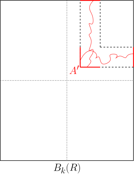
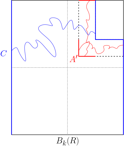
where the second inequality is Jensen’s. Hence it is enough to construct an event $A^{\prime}$, measurable with respect to $\mathcal{F}_{\mathcal{S}^{\prime}}$, such that $\textrm{Cross}_{k}(R)$ becomes substantially more likely if $A^{\prime}$ occurs (see Figure 1 for an illustration).

Define

$$A^{\prime}:=\Big{\{}\{R/4\}\times[R/4,R/2]\stackrel{{\scriptstyle[R/4,R]\times[R/4,R/2]}}{{\longleftrightarrow}}\{R\}\times[R/4,R/2]\Big{\}}$$

$$\qquad\qquad\cap\Big{\{}[R/4,R/2]\times\{R/4\}\stackrel{{\scriptstyle[R/4,R/2]\times[R/4,kR]}}{{\longleftrightarrow}}[R/4,R/2]\times\{kR\}\Big{\}},$$

which is measurable with respect to $\mathcal{F}_{\mathcal{S}^{\prime}}$. By the FKG inequality and symmetry (and an obvious event inclusion), $\mathbb{P}_{\ell}[A^{\prime}]\geq\mathbb{P}_{\ell}[\textrm{Cross}_{1/(8k)}(kR)]^{2}$. Define also the events

$$B_{1} :=\Big{\{}\{-R\}\times[R/2,3R/4]\stackrel{{\scriptstyle[-R,R/2]\times[R/2,3R/4]}}{{\longleftrightarrow}}\{R/2\}\times[R/2,3R/4]\Big{\}}$$

$$B_{2} :=\Big{\{}\{3R/4\}\times[-kR,kR]\stackrel{{\scriptstyle[3R/4,R]\times[-kR,kR]}}{{\longleftrightarrow}}\{R\}\times[-kR,kR]\Big{\}}$$

which are defined on domains separated by a sup-norm distance at least $r$ (recall that $R\geq 8r$), and are translated copies of, respectively, $\textrm{Cross}_{1/6}(3R/2)$ and $\textrm{Cross}_{8k}(R/8)$. Finally, define

$$C\!:=\!\!\Big{\{}\!\{-R\}\times[-kR,kR]\stackrel{{\scriptstyle B_{k}(R)}}{{\longleftrightarrow}}\big{(}\{R/2\}\times[R/2,kR]\big{)}\!\cup\!\big{(}[R/2,R]\times\{R/2\}\big{)}\!\cup\!\big{(}\{R\}\times[-kR,R/2]\big{)}\!\Big{\}}$$

and observe (i) $\textrm{Cross}_{k}(R)\subseteq C$, (ii) on $A^{\prime}$, $\textrm{Cross}_{k}(R)=C$, and (iii) $B_{1}\cap B_{2}^{\mathsf{c}}\subseteq C\setminus\textrm{Cross}_{k}(R)$. Hence

$$\mathbb{P}_{\ell}[\textrm{Cross}_{k}(R)|A^{\prime}]-\mathbb{P}_{\ell}[\textrm{Cross}_{k}(R)] =\mathbb{P}_{\ell}[C|A^{\prime}]-\mathbb{P}_{\ell}[\textrm{Cross}_{k}(R)]\geq\mathbb{P}_{\ell}[C]-\mathbb{P}_{\ell}[\textrm{Cross}_{k}(R)]$$

$$=\mathbb{P}_{\ell}[C\setminus\textrm{Cross}_{k}(R)]\geq\mathbb{P}_{\ell}[B_{1}\cap B_{2}^{\mathsf{c}}]=\mathbb{P}_{\ell}[B_{1}](1-\mathbb{P}_{\ell}[B_{2}])$$

$$\geq\mathbb{P}_{\ell}[\textrm{Cross}_{1/(8k)}(kR)]\big{(}1-\mathbb{P}_{\ell}[\textrm{Cross}_{8k}(R/8)]\big{)},$$

where the second step is by the FKG inequality, the penultimate step uses the independence of the events $B_{1}$ and $B_{2}$, and the final step is an obvious event inclusion. Applying (3.13) (with $A=\textrm{Cross}_{k}(R)$ and $\mathcal{G}=\mathcal{F}_{\mathcal{E}^{\prime}}$) gives (3.12).

Figure 1. An illustration of the proof of (3.12). The first panel shows the event $A^{\prime}$. The second illustrates how, on $A^{\prime}$, the event $C$ is equivalent to $\textrm{Cross}_{k}(R)$. The third shows how the crossing given by $B_{1}$, combined with the dual crossing given by $B_{2}^{\mathsf{c}}$, realises $C$ but not $\textrm{Cross}_{k}(R)$.

∎

Remark 3.9.

Similarly to in Section 1.5.3, combining Propositions 1.20 and 3.8 yields a general lower bound on the revealments of increasing events. We omit the proof, but the result is the following. Let $\ell\in\mathbb{R}$, let $R\geq r$, let $A$ be an increasing continuity event supported on $B(R)$, let $s>0$, and let $\mathcal{A}\in\mathcal{A}_{s}$ be an algorithm determining $A$. Then there exists a $c>0$ depending only on $d$ such that

$$\max_{S\in\mathcal{S}_{s}}\textrm{Rev}(S)\geq\frac{c\big{(}(\int q/\|q\|_{2})\min\{1,(s/r)^{d}\}\textrm{Var}_{\ell}[\mathds{1}_{A}]\big{)}^{2/3}}{\mathbb{P}_{\ell}[A]^{1/3}R^{d/3}}$$

where the revealments $\textrm{Rev}(S)$ are under $\mathbb{P}_{\ell}$.

One can also prove a lower bound on $\max_{S\in\mathcal{S}^{\prime}}\textrm{Rev}(S)$ for general $\mathcal{S}^{\prime}\subset\mathcal{S}_{s}$, analogous to Proposition 1.26, however in that case we would need $q\geq 0$ (for the same reason as explained in Remark 3.7 above) and also the refinement to Proposition 1.23 mentioned in Remark 5.3.

3.4. Proof of Lemma 3.4

For the first statement, it is enough to prove that

(3.14) $$\liminf_{R\to\infty}\mathbb{P}_{\ell_{c}}[\textrm{Cross}_{5}(R)]>0$$

since then the result follows by the continuity of $\ell\mapsto\mathbb{P}_{\ell}[\textrm{Cross}_{5}(R)]$. By a classical bootstrapping argument [33, Section 5.1] (and Lemma 4.2 below), there are $c_{1},\varepsilon>0$ such that

(3.15) $$\mathbb{P}_{\ell}[\textrm{Cross}_{5}(3R)]\leq c_{1}\big{(}\mathbb{P}_{\ell}[\textrm{Cross}_{5}(R)]^{2}+R^{-\varepsilon}\big{)}$$

for $\ell\in\mathbb{R}$ and $R$ sufficiently large. A consequence of (3.15) and the continuity of $\ell\mapsto\mathbb{P}_{\ell}[\textrm{Cross}_{5}(R)]$ is that

$$\liminf_{R\to\infty}\mathbb{P}_{\ell}[\textrm{Cross}_{5}(R)]<1/c_{1}\quad\implies\quad\liminf_{R\to\infty}\mathbb{P}_{\ell^{\prime}}[\textrm{Cross}_{5}(R)]=0\quad\text{for some }\ell^{\prime}>\ell.$$

Covering the annulus $\Lambda_{5R}\setminus\Lambda_{3R}$ with $2d$ symmetric copies of $B_{5}(R)$, one can find a finite collection of copies $A_{i}$ of $\textrm{Cross}_{5}(R)$ such that $\{\Lambda_{1}\longleftrightarrow\infty\}\subseteq A_{1}(3R,5R)\subseteq\cup_{i}A_{i}$. Hence we also have

$$\liminf_{R\to\infty}\mathbb{P}_{\ell^{\prime}}[\textrm{Cross}_{5}(R)]=0\quad\implies\quad\mathbb{P}_{\ell^{\prime}}[\Lambda_{1}\longleftrightarrow\infty]=0\quad\implies\quad\ell^{\prime}\leq\ell_{c},$$

and so we deduce (3.14).

The RSW estimates in the second statement are a general property of stationary planar percolation models with positive associations and the symmetry in Assumption 1.1 [35].

For the third statement, consider first the case $\mathbb{X}=\mathbb{Z}$. Under Assumption 1.1 the covariance kernel $K$ is strictly positive definite, which implies that every compactly supported event is a continuity event. So let us assume $\mathbb{X}=\mathbb{R}$. Letting $g$ be a smooth function, since $f$ is $C^{2}$-smooth and $(f(x),\nabla f(x),\nabla^{2}f(x))$ is non-degenerate, by [1, Lemma 11.2.11], for any $\ell\in\mathbb{R}$, almost surely there are no critical points of $f$ in the set $\{f+g+\ell=0\}$. The same holds for the field restricted to a smooth hypersurface. Hence, almost surely, on event $\{f+g+\ell\in\textrm{Cross}_{k}(R)\}$ or $\{f+g+\ell\in A_{1}(r,R)\}$, there exist a witness path $\gamma$ and a $\delta>0$ such that $f+g+\ell>\delta$ on the image of $\gamma$. Hence the event is still verified by the field $f+g+\ell\pm\delta^{\prime}$ for all $\delta^{\prime}\leq\delta$, which implies continuity.

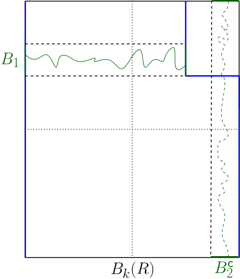
3.5. Proof of Lemma 3.6

We begin by introducing some notation. We make a distinction between the set of boxes that are revealed by an algorithm, and the set $V\subset\mathbb{R}^{d}$ on which the field $f$ is determined by an algorithm. More precisely, for $V\subset\mathbb{R}^{d}$ and a set of boxes $\mathcal{P}\subset\mathcal{S}_{s}$, we say that $f$ is determined on $V$ using $\mathcal{P}$ if $f|_{V}=(\sum_{S\in\mathcal{P}}f_{S})|_{V}$, or equivalently, if $((\bigcup_{S\in\mathcal{S}_{s}\setminus\mathcal{P}}\textrm{Supp}(q\star\mathbbm{1}_{S}))\cap V=\emptyset$.

Distinct boxes $S,S^{\prime}\in\mathcal{S}_{r}$ are adjacent if their closures have non-empty intersection. For a set of boxes $\mathcal{P}\subset\mathcal{S}_{r}$ define its outer boundary

$$\partial^{+}P:=\{S\in\mathcal{S}_{r}\setminus\mathcal{P}:\text{ $S$ is adjacent to a box $S^{\prime}\in\mathcal{P}$ }\},$$

so in particular $\partial^{+}\{S\}$ are the boxes adjacent to $S$. Define also the interior $\textrm{int}(\mathcal{P}):=\{S\in\mathcal{P}:\partial^{+}\{S\}\subseteq\mathcal{P}\}$. Note that, since $q$ is supported on $\Lambda_{r}$, $f$ is determined on $\textrm{int}(\mathcal{P})$ using $\mathcal{P}$. A primal (resp. dual) path will designate a path in $\{f\geq 0\}$ (resp. $\{f\leq 0\}$). An interface inside a compact set $K$ will designate, in the case $\mathbb{X}=\mathbb{R}$, a connected component of $\{f=0\}\cap K$. In the case $\mathbb{X}=\mathbb{Z}$, an interface will be a self-avoiding edge path $(e_{1},...,e_{k})$ inside $K$ such that

• for any $i=1,...,k$, the endpoints of $e_{i}$ are in $\{f\geq 0\}$,

• for any $i$, there exists a vertex $v\in\mathbb{Z}^{d}$ such that $e_{i}$ and $v$ are at distance smaller or equal to $1$ for the sup norm, and $f(v)\leq 0$, and

• the path is maximal for these properties.

In both settings, we say that these paths are contained in a set of boxes $\mathcal{P}\subset\mathcal{S}_{r}$ if they are contained in $\cup_{S\in\mathcal{P}}S$. The left and right sides of $B_{k}(R)$ are respectively $\{-R\}\times[-kR,kR]^{d-1}$ and $\{R\}\times[-kR,kR]^{d-1}$, and if $d=2$ the top and bottom sides are defined similarly.

For the first statement consider the following algorithm:

• Reveal every box that intersects $\Lambda_{1}$ as well as all adjacent boxes.

• Iterate the following steps:

  • Let $\mathcal{W}\subset\mathcal{S}_{r}$ be the boxes that have been revealed.

  • Identify the set $\mathcal{U}\subseteq\partial^{+}(\textrm{int}(\mathcal{W}))$ such that, for each $S\in\mathcal{U}$, there is a primal path contained in $\textrm{int}(\mathcal{W})\cap\Lambda_{R}$ between $\Lambda_{1}$ and the boundary of $S$ (measurable since $f$ is determined on $\textrm{int}(\mathcal{W})$). In other words, $\mathcal{U}$ contains all boxes on which $f$ is not yet determined but which are connected to $\Lambda_{1}$ by a primal path in $\Lambda_{R}$ that has been determined.

  • If $\mathcal{U}$ is empty end the loop. Otherwise reveal the boxes in $\partial^{+}\mathcal{U}\setminus\mathcal{W}$.

• If $\textrm{int}(\mathcal{W})\cap\Lambda_{R}$ contains a primal path between $\Lambda_{1}$ and $\partial\Lambda_{R}$ output $1$, otherwise output $0$.

This algorithm determines $A_{1}(R)$ since $\textrm{int}(\mathcal{W})$ eventually contains all the components of $\{f\geq 0\}\cap\Lambda_{R}$ that intersect $\Lambda_{1}$. To estimate the sum of revealments $\textrm{Rev}(S)$, a box $S$ is revealed if and only if either (i) it is adjacent to a box that intersects $\Lambda_{1}$, or (ii) there is a primal path in $\Lambda_{R}$ between $\Lambda_{1}$ and a box adjacent to $S$. If $S=v+[0,r)^{2}$ and $\Lambda_{1}\cap(v+\Lambda_{2r})=\emptyset$ then the latter implies the occurrence of $\Lambda_{1}\longleftrightarrow v+\Lambda_{2r}$. Summing over $S$ gives

$$\sum_{S\in\mathcal{S}_{r}}\textrm{Rev}(S)\leq\sum_{v\in r\mathbb{Z}^{d}\cap\Lambda_{R+2r}}\mathbb{P}_{p}[\Lambda_{1}\longleftrightarrow v+\Lambda_{2r}].$$

The second algorithm is the following

• Define $L$ to be $\{-R\}\times[-kR,kR]^{d-1}$, and reveal every box that intersects $L\cap B_{k}(R)$, as well as all adjacent boxes.

• Iterate the following steps:

  • Let $\mathcal{W}\subset\mathcal{S}_{r}$ be the boxes that have been revealed.

  • Identify the set $\mathcal{U}\subseteq\partial^{+}(\textrm{int}(\mathcal{W}))$ such that, for each $S\in\mathcal{U}$, there is a primal path contained in $\textrm{int}(\mathcal{W})\cap B_{k}(R)$ between $L\cap B_{k}(R)$ and the boundary of $S$.

  • If $\mathcal{U}$ is empty end the loop. Otherwise reveal the boxes in $\partial^{+}\mathcal{U}\setminus\mathcal{W}$.

• If $\textrm{int}(\mathcal{W})\cap B_{k}(R)$ contains a primal path between the left and right sides of $B_{k}(R)$ output $1$, otherwise output $0$.

A box $S\in\mathcal{S}_{r}$ such that $d_{\infty}(S,B_{k}^{+}(R))\leq r$ is only revealed if there is a primal path in $B_{k}(R)$ between $L$ and a box adjacent to $S$, which implies the occurrence of (a translation of) the event $A_{1}(2r,d)$, where $d$ is the distance from the centre of $S$ to $L$. Since $d$ is at least $R-2r$, $\textrm{Rev}(S)\leq\mathbb{P}_{\ell}[A_{1}(2r,R-2r)]$ as required.

The final algorithm (specific to $d=2$) is:

• Define $L_{1}=[-R,R]\times\{-kR\}$ and $L_{2}=\{-R\}\times[-kR,kR]$, and reveal every box that intersects $(L_{1}\cup L_{2})\cap B_{k}(R)$, as well as all adjacent boxes.

• Iterate the following steps:

  • Let $\mathcal{W}\subset\mathcal{S}_{r}$ be the boxes that have been revealed.

  • Identify the set $\mathcal{U}\subseteq\partial^{+}(\textrm{int}(\mathcal{W}))$ such that, for each $S\in\mathcal{U}$, there is an interface contained in $\textrm{int}(\mathcal{W})\cap B_{k}(R)$ between $(L_{1}\cup L_{2})\cap B_{k}(R)$ and the boundary of $S$.

  • If $\mathcal{U}$ is empty end the loop. Otherwise reveal the boxes in $\partial^{+}\mathcal{U}\setminus\mathcal{W}$.

• If $\textrm{int}(\mathcal{W})\cap B_{k}(R)$ contains a primal (resp. dual) path between the left and right (resp. top and bottom) sides of $B_{k}(R)$ terminate with output $1$ (resp. $0$).

• Since $\textrm{int}(\mathcal{W})$ contains interfaces inside $B_{k}(R)$ that intersect $L_{1}\cap L_{2}$ and the algorithm has not yet terminated, exactly one of $\{f\geq 0\}\cap B_{k}(R)$ or $\{f\leq 0\}\cap B_{k}(R)$ has an interface that intersects all four sides of $B_{k}(R)$. Partition $B_{k}(R)$ into regions $(P_{i})$ using the interfaces inside $\cap B_{k}(R)$ that intersect $L_{1}\cup L_{2}$. Let $\mathbb{A}$ to be the region $P_{i}$ which contains the top-left corner of $B_{k}(R)$, and set $\mathcal{C}=1$ (resp. $\mathcal{C}=0$) if $f$ is positive (resp. negative) on $P_{i}$. Then iterate the following:

  • If $\mathbb{A}$ contains a path in $B_{k}(R)$ between its left and right sides terminate with output $\mathcal{C}$.

  • Change the value of $\mathcal{C}$ (from $0$ to $1$ or $1$ to $0$), and add to $\mathbb{A}$ the region $P_{i}$ that is adjacent to it.

The final loop is illustrated in Figure 2; it terminates almost surely since there are a finite number of interfaces in $B_{k}(R)$ (recall that when $\mathbb{X}=\mathbb{R}$, $f$ is $C^{1}$-smooth). Note that the algorithm does not necessarily reveal all components of $\{f=0\}$ inside $B_{k}(R)$ – any components which are closed loops or only touch the top and right sides of $B_{k}(R)$ are not revealed – but these do not affect whether $\textrm{Cross}_{k}(R)$ occurs.

Figure 2. The final loop of the algorithm in the proof of the third statement of Lemma 3.6; this loop occurs when there is no left-right or top-bottom paths in $\{f=0\}\cap B_{k}(R)$. In this example the loop expands the area $\mathbb{A}$ three times in order to determine the sign $\mathcal{C}$ of the crossing.

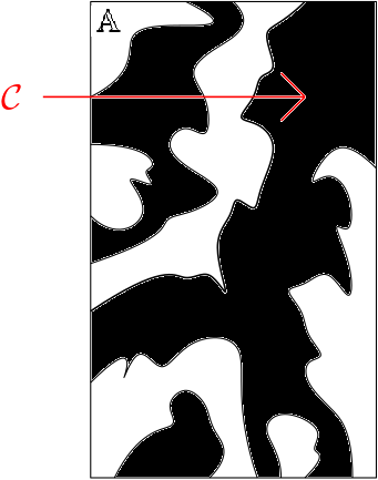
To estimate the revealments of this algorithm, a box $S\in\mathcal{S}_{r}$ such that $d_{\infty}(S,B_{k}^{\dagger}(R))\leq r$ is only revealed if there is an interface in $B_{k}(R)$ between $L_{1}\cap L_{2}$ and a box adjacent to $S$, which implies the occurrence of (a translation of) the event $A_{2}(2r,d^{\prime})$, where $d^{\prime}$ is the distance from the centre of $S$ to $L_{1}\cap L_{2}$. Since $d^{\prime}$ is at least $R-2r$, $\textrm{Rev}(S)\leq\mathbb{P}_{\ell}[A_{2}(2r,R-2r)]$ as required.

4. Extension to models with unbounded range of dependence

In this section we use approximation arguments to extend our results to models with unbounded range of dependence. We shall assume that $f$ satisfies Assumption 1.1 with parameter $\beta>d$, and also that (POS) holds.

As well as the intermediate propositions 3.1–3.3, in this section we shall additionally rely on a slight variant of Proposition 3.3 which applies outside the self-dual case:

Proposition 4.1.

Suppose $r>0$ is such that $q$ is supported on $\Lambda_{r}$. Then for $k\geq 1$ there exists $c=c(k)>0$ such that, for $\ell\in\mathbb{R}$ and $R\geq 8r>0$,

$$\frac{d^{-}}{d\ell}\mathbb{P}_{\ell}[\textrm{Cross}_{k}(R)]\geq\frac{c}{\|q\|_{2}}\frac{\mathbb{P}_{\ell}[\textrm{Cross}_{k}(R)]\big{(}1-\mathbb{P}_{\ell}[\textrm{Cross}_{k}(R)]\big{)}}{\frac{r}{R}\sum_{i=2}^{R/r}\mathbb{P}_{\ell}[A_{1}(2r,ir)]}.$$

Proof of Proposition 4.1.

The proof is very similar to that of Proposition 3.3. Similarly to in Lemma 3.6, for every $k\geq 1$, $\ell\in\mathbb{R}$, and $R\geq 4r>0$, there is an algorithm in $\mathcal{A}_{r}$ determining $\textrm{Cross}_{k}(R)$ such that, under $\mathbb{P}_{\ell}$,

$$\max_{S\in\mathcal{S}_{r}}\textrm{Rev}(S)\leq\frac{4r}{R}\sum\limits_{i=2}^{R/r}\mathbb{P}_{\ell}[A_{1}(2r,ir)].$$

Indeed we can define an algorithm which initially reveals a line $L$ of the form $L=\{ir\}\times[-kR,kR]^{d-1}$ for some uniform random $i$ in the given range. Then the algorithm reveals sequentially the set which is connected to that line through primal paths until the occurrence of the crossing event is determined. Then we deduce the result by applying Proposition 3.8 (in the case $s=r$, $\mathcal{S}^{\prime}=\mathcal{S}_{s}$, and $A=\textrm{Cross}_{k}(R)$) to this algorithm. ∎

We shall also need an approximation lemma that allows us to compare a general $f=q\star W$ to a field with finite-range dependence. Fix a smooth symmetric cutoff function $\varphi:\mathbb{R}\to[0,1]$ such that $\varphi(x)=1$ for $\|x\|_{\infty}\leq 1/2$, $\varphi(x)=0$ for $\|x\|_{\infty}\geq 1$. For $r>0$ define

(4.1) $$f_{r}:=q_{r}\star W$$

where $q_{r}(x):=q(x)\varphi(|x|/r)$. Note that $q_{r}$ is supported on $\Lambda_{r}$, and also, since $q\in L^{1}(\mathbb{X}^{d})\cap L^{2}(\mathbb{X}^{d})$, as $r\to\infty$,

(4.2) $$\|q_{r}\|_{2}\to\|q\|_{2}\qquad\text{and}\qquad\int q_{r}\to\int q.$$

Using the fact that Assumption 1.1 and (POS) hold for $f$, we can verify that these hold also for $f_{r}$ for sufficiently large $r$ (on the other hand, deducing that (PA) holds for $f_{r}$ if it holds for $f$ seems difficult but we do not need it). In particular, in the self-dual case $\ell_{c}(f_{r})=\ell_{c}(f)=0$.

The following lemma, essentially taken from [43], allows us to compare $f$ and $f_{r}$. We give details on the proof at the end of the section.

Lemma 4.2.

There exist $c_{1},c_{2}>0$ such that, for $r,R\geq 2$, increasing event $A$ measurable with respect to $f|_{B(R)}$, and $\ell\in\mathbb{R}$,

$$\left|\mathbb{P}_{\ell}[f\in A]-\mathbb{P}_{\ell}[f_{r}\in A]\right|\leq c_{1}\big{(}R^{d/2}(\log R)r^{-(\beta-d/2)}+e^{-c_{2}(\log R)^{2}}\big{)}.$$

The same conclusion holds if $A$ is the intersection of one increasing and one decreasing event which are both measurable with respect to $f|_{B(R)}$.

We are now ready to prove Theorem 1.8:

Proof of Theorem 1.8.

In the proof $c>0$ are constants that depend only on $f$ (and the choice of the cutoff function $\varphi$ in (4.1)) and may change from line to line.

The bound $\eta_{1}\leq d-1$, and also $\eta_{1}\leq 1/2$ if $d=2$ and (PA) holds, are rather classical; in fact they are true for any $\beta>d$. For the former, combining $\mathbb{P}_{\ell_{c}}[\textrm{Cross}_{5}(R)]\geq\delta$ (the first statement of Lemma 3.4) with the union bound applied along the hyperplane $\{0\}\times[-kR,kR]$ gives $\mathbb{P}_{\ell_{c}}[A_{1}(R)]\geq cR^{-(d-1)}$. For the latter, by combining the RSW estimates (the second statement of Lemma 3.4) with Lemma 4.2 one can deduce (see [5, 43] for similar arguments)

$$\mathbb{P}_{\ell_{c}}\big{[}\{-R\}\times[-R,R]\stackrel{{\scriptstyle B_{1}(R)}}{{\operatorname*{\Longleftrightarrow}}}\{R\}\times[-R,R]\big{]}\geq c\big{(}1-R^{1-(\beta-1)}(\log R)\big{)}\geq c/2$$

for sufficiently large $R$. By the union bound applied along $\{0\}\times[-R,R]$ this implies $\mathbb{P}_{\ell_{c}}[A_{2}(R)]\geq cR^{-1}$, and given (3.1) we see that $\mathbb{P}_{\ell_{c}}[A_{1}(R)]\geq cR^{-1/2}$.

We now prove the remaining bounds, beginning with the first statement. Fix $1>\alpha>\frac{d/2}{\beta-d/2}$ and $\eta_{1}>\eta^{\ast}>0$ (if $\eta_{1}=0$ there is nothing to prove). Then by monotonicity in $\ell$, the union bound, and the definition of $\eta_{1}$,

$$\mathbb{P}_{\ell}[A_{1}(r,R)]\leq\mathbb{P}_{\ell_{c}}[A_{1}(r,R)]\leq cr^{d-1}\mathbb{P}_{\ell_{c}}[A_{1}(R-r)]\leq r^{d-1}R^{-\eta^{\ast}}$$

for all $\ell\leq\ell_{c}$, $R$ sufficiently large, and $r\in[1,R/2]$. Set $r=R^{\alpha}$. Then by an integral comparison,

$$\frac{r}{R}\sum_{i=2}^{R/r}\mathbb{P}_{\ell_{c}}[A_{1}(2r,ir)] \leq cr^{-\eta^{\ast}+(d-1)}\times\frac{r}{R}\sum_{i=2}^{R/r}i^{-\eta^{\ast}}$$

$$\leq cr^{-\eta^{\ast}+(d-1)}(R/r)^{-\min\{\eta^{\ast},1\}}(\log(R/r))$$

$$\leq c(\log R)\big{(}R^{\alpha(d-1-\eta^{\ast})-(1-\alpha)\min\{\eta^{\ast},1\}}\big{)}$$

for $\ell\leq\ell_{c}$ and large $R$. Consider the field $f_{r}$ defined in (4.1). By Lemma 4.2,

$$\mathbb{P}_{\ell}[f_{r}\in A_{1}(r^{\prime},R)]\leq\mathbb{P}_{\ell}[A_{1}(r^{\prime},R)]+cR^{d/2-\alpha(\beta-d/2)}(\log R)+ce^{-c(\log R)^{2}}$$

for $\ell\leq\ell_{c}$ and $2\leq r^{\prime}\leq R$, and hence

$$\frac{r}{R}\sum_{i=2}^{R/r}\mathbb{P}_{\ell}[f_{r}\in A_{1}(2r,ir)]\leq c(\log R)\big{(}R^{\alpha(d-1-\eta^{\ast})-(1-\alpha)\min\{\eta^{\ast},1\}}+R^{d/2-\alpha(\beta-d/2)}\big{)}$$

for $\ell\leq\ell_{c}$ and large $R$. Moreover, by Lemma 3.4 there are $\delta>0$ and $\ell^{\prime}=\ell^{\prime}(R)\leq\ell_{c}$ such that $\mathbb{P}_{\ell^{\prime}}[\textrm{Cross}_{5}(R)]=\delta$. Hence, again by Lemma 4.2,

$$\mathbb{P}_{\ell^{\prime}}[f_{r}\in\textrm{Cross}_{5}(R)]\big{(}1-\mathbb{P}_{\ell^{\prime}}[f_{r}\in\textrm{Cross}_{5}(R)]\big{)}\geq\delta(1-\delta)-cR^{d/2-\alpha(\beta-d/2)}(\log R)\geq\delta(1-\delta)/2$$

for large $R$, where we used that $\alpha>\frac{d/2}{\beta-d/2}$.

We now apply Propositions 3.2 and 4.1 to the field $f_{r}$ at the sequence of levels $\ell^{\prime}(R)\leq\ell_{c}$. First, by Proposition 3.2 (recalling (4.2))

(4.3) $$\frac{d}{d\ell}\mathbb{P}_{\ell}[f_{r}\in\textrm{Cross}_{5}(R)]\Big{|}_{\ell=\ell^{\prime}} \geq\frac{c\delta(1-\delta)}{\|q_{r}\|_{2}}\Big{(}\frac{r}{R}\sum_{i=2}^{R/r}\mathbb{P}_{\ell^{\prime}}[f_{r}\in A_{1}(2r,ir)]\Big{)}^{-1}$$

$$\geq c(\log R)^{-1}\big{(}R^{\alpha(d-1-\eta^{\ast})-(1-\alpha)\min\{\eta^{\ast},1\}}+R^{d/2-\alpha(\beta-d/2)}\big{)}^{-1}$$

for large $R$. Similarly, by Proposition 3.1,

(4.4) $$\frac{d}{d\ell}\mathbb{P}_{\ell}[f_{r}\in\textrm{Cross}_{5}(R)]\Big{|}_{\ell=\ell^{\prime}} \leq cR^{d/2}\Big{(}\mathbb{P}_{l^{\prime}}[f_{r}\in A_{1}(2r,R)]\Big{)}^{1/2}$$

$$\leq cR^{d/2}\big{(}R^{-\eta^{\ast}+\alpha(d-1)}+R^{d/2-\alpha(\beta-d/2)}(\log R)\big{)}^{1/2}$$

$$\leq c\sqrt{\log R}\big{(}R^{d/2-\eta^{\ast}/2+\alpha(d-1)/2}+R^{3d/4-\alpha(\beta-d/2)/2}\big{)}$$

for large $R$, where we used that $\sqrt{a+b}\leq\sqrt{a}+\sqrt{b}$ for $a,b>0$. Comparing (4.3) and (4.4) and expanding the brackets we deduce that at least one of the exponents

$$E_{1}:=\big{(}3d/4-\alpha(\beta-d/2)/2\big{)}+\big{(}d/2-\alpha(\beta-d/2)\big{)}$$

$$E_{2}:=\big{(}d/2-\eta^{\ast}/2+\alpha(d-1)/2\big{)}+\big{(}d/2-\alpha(\beta-d/2)\big{)}$$

$$E_{3}:=\big{(}d/2-\eta^{\ast}/2+\alpha(d-1)/2\big{)}+\big{(}\alpha(d-1-\eta^{\ast})-(1-\alpha)\min\{\eta^{\ast},1\}\big{)}$$

$$E_{4}:=\big{(}3d/4-\alpha(\beta-d/2)/2\big{)}+\big{(}\alpha(d-1-\eta^{\ast})-(1-\alpha)\min\{\eta^{\ast},1\}\big{)}$$

must be non-negative. The first is equivalent to $\alpha\leq\frac{5d}{6(\beta-d/2)}$. The second implies that $\eta^{\ast}\leq\frac{d}{3}+\alpha(d-1)$, assuming that $\alpha>\frac{5d}{6(\beta-d/2)}$. The third is equivalent to either $\eta^{\ast}\leq\frac{d}{3}+\alpha(d-1)$ (if $\eta^{\ast}\leq 1$) or $\eta^{\ast}\leq\frac{d-2+\alpha(3d-1)}{1+2\alpha}$ (if $\eta^{\ast}>1$). Finally, the fourth implies either $\eta^{\ast}\leq\frac{d}{3}+\alpha(d-1)$ (if $\eta^{\ast}\leq 1$, assuming that $\alpha>\frac{5d}{6(\beta-d/2)}$) or $\alpha\leq\frac{3d-4}{2\beta-5d+4}$ (if $\eta^{\ast}>1$). One can check that, since $d\geq 3$, $\frac{5d}{6(\beta-d/2)}<\frac{3d-4}{2\beta-5d+4}$ and $\frac{d}{3}+\alpha(d-1)<\frac{d-2+\alpha(3d-1)}{1+2\alpha}$. Hence we conclude that if $\alpha>\frac{3d-4}{2\beta-5d+4}$ then $\eta^{\ast}\leq\frac{d-2+\alpha(3d-1)}{1+2\alpha}$. Sending $\alpha\to\frac{3d-4}{2\beta-5d+4}$ from above gives the result.

The proof of the remaining statements are similar, and closer to the arguments in Section 3. For the second statement, fix $1>\alpha>\frac{3d/2-1}{\beta-d/2}$ and $\eta_{1}>\eta^{\ast}>0$. As in the proof of the first statement,

(4.5) $$\mathbb{P}_{\ell_{c}}[A_{1}(2r,R)]\leq r^{d-1}R^{-\eta^{\ast}}$$

for large $R$ and $r\in[1,R/4]$. Now let $r=R^{\alpha}$. Since we have the a priori bound $\mathbb{P}_{\ell_{c}}[A_{1}(1R)]\geq cR^{-(d-1)}$ (from the start of the proof), by Lemma 4.2

(4.6) $$|\mathbb{P}_{\ell_{c}}[f_{r}\in A_{1}(r^{\prime},R^{\prime})]-\mathbb{P}_{\ell_{c}}[A_{1}(r^{\prime},R^{\prime})]| \leq cR^{d/2-\alpha(\beta-d/2)}(\log R)+ce^{-c(\log R)^{2}}$$

$$\leq\mathbb{P}_{\ell_{c}}[A_{1}(r^{\prime},R^{\prime})]/2$$

for large $R$ and $1\leq r^{\prime}\leq R^{\prime}\leq R$, where we used that $d/2-\alpha(\beta-d/2)\leq-(d-1)$ by the definition of $\alpha$.

Similarly to (4.6) we also have

$$|\mathbb{P}_{\ell^{\prime}}[f_{r}\in A_{1}(R)]-\mathbb{P}_{\ell^{\prime}}[A_{1}(R)]| \leq cR^{d/2-\alpha(\beta-d/2)}(\log R)+ce^{-c(\log R)^{2}}$$

$$\leq\mathbb{P}_{\ell_{c}}[A_{1}(R)]=\mathbb{P}_{\ell^{\prime}}[A_{1}(R)]/2.$$

Then applying Proposition 3.1 to the field $f_{r}$, for large $R$,

$$\mathbb{P}_{\ell_{c}}[A_{1}(R)] =\mathbb{P}_{\ell^{\prime}}[A_{1}(R)]-\mathbb{P}_{\ell_{c}}[A_{1}(R)]\leq 2(\mathbb{P}_{\ell^{\prime}}[f_{r}\in A_{1}(R)]-\mathbb{P}_{\ell_{c}}[f_{r}\in A_{1}(R)])$$

$$\leq\frac{2r^{d/2}(\ell^{\prime}-\ell_{c})}{\int q}\sqrt{\mathbb{P}_{\ell^{\prime}}[A_{1}(R)]\!\!\sum_{v\in r\mathbb{Z}^{d}\cap\Lambda_{R+2r}}\!\!\mathbb{P}_{\ell_{c}}[\Lambda_{2r}\longleftrightarrow v+\Lambda_{2r}]}$$

$$\leq\frac{2(\ell^{\prime}-\ell_{c})}{\int q}R^{\alpha d/2}\sqrt{R^{-\eta^{\ast}}R^{\max\{0,\alpha(d-1),-\alpha+d-2\eta^{\ast}\}}(\log R)}.$$

Comparing with (3.3) implies that $\alpha d-\eta^{\ast}+\max\{\alpha(d-1),-\alpha+d-2\eta^{\ast}\}\geq 0$, and so $\eta^{\ast}\leq\max\{d/3+\alpha(d-1)/3,\alpha(2d-1)\}$, and sending $\alpha\to\frac{3d/2-1}{\beta-d/2}$ from above gives the result.

Finally, consider the third statement. Fix $1>\alpha>\frac{5}{3(\beta-1)}$ and $r=R^{\alpha}$. By the RSW estimates (the second statement of Lemma 3.4) and Lemma 4.2,

$$\mathbb{P}_{\ell_{c}}[f_{r}\in\textrm{Cross}_{1}(R)]\big{(}1-\mathbb{P}_{\ell_{c}}[f_{r}\in\textrm{Cross}_{1}(R)]\big{)}\leq c-cR^{1-\alpha(\beta-1)}(\log R)<c/2$$

for large $R$. Then by Propositions 3.2 and 3.3 we have, for large $R$,

$$c\mathbb{P}_{\ell_{c}}[f_{r}\in A_{2}(2r,R-2r)]^{-1}\leq\frac{d}{d\ell}\mathbb{P}_{\ell}[f_{r}\in\textrm{Cross}_{1}(R)]\Big{|}_{\ell=\ell_{c}}\leq cR\sqrt{\mathbb{P}_{\ell_{c}}[f_{r}\in A_{2}(2r,R-2r)]}$$

which gives $\mathbb{P}_{\ell_{c}}[f_{r}\in A_{2}(2r,R-2r)]\geq cR^{-2/3}$ for large $R$. Applying the union bound and Lemma 4.2 (valid since $A_{2}(3\sqrt{2}r,R)$ is the intersection of an increasing and a decreasing event) yields

$$\mathbb{P}_{\ell_{c}}[A_{2}(R-2r)]\geq cr^{-1}\mathbb{P}_{\ell_{c}}[A_{2}(2r,R-2r)]\geq cR^{-\alpha}\big{(}R^{-2/3}-R^{1-\alpha(\beta-1)}(\log R)\big{)}.$$

Sending $\alpha\to\frac{5}{3(\beta-1)}$ from above gives that, for every $\varepsilon>0$,

(4.7) $$\mathbb{P}_{\ell_{c}}[A_{2}(R)]\geq c_{2}R^{-2/3-5/(3(\beta-1))-\varepsilon}.$$

for $c_{2}=c_{2}(\varepsilon)>0$ and large $R$. Hence by (3.1) (recall that here $\mathbb{X}=\mathbb{R}$),

(4.8) $$\mathbb{P}_{\ell_{c}}[A_{1}(R)]\geq(\mathbb{P}_{\ell_{c}}[A_{2}(R)])^{1/2}\geq c_{3}R^{-1/3-5/(6(\beta-1))-\varepsilon/2}$$

for $c_{3}=c_{3}(\varepsilon)>0$ and large $R$, which gives the result. ∎

4.1. The approximation lemma

To finish the section we give some details on the approximation result in Lemma 4.2.

Proof of Lemma 4.2.

We first observe that $g:=f-f_{r}=(q-q_{r})\star W$ is a stationary Gaussian field satisfying

$$\mathbb{E}[g(0)^{2}]=\int_{x\in\mathbb{R}^{d}}(q-q_{r})^{2}(x)\,dx=\int_{|x|>r/2}q(x)^{2}(1-\varphi(|x/r|))^{2}\,dx\leq\int_{|x|>r/2}q(x)^{2}\leq c_{1}r^{d-2\beta},$$

for some $c_{1}>0$ and we used that $|q(x)|\leq c|x|^{-\beta}$ by Assumption 1.1. Similarly, in the case that $f$ is continuous, $g$ is $C^{1}$-smooth and for every direction $v\in\mathbb{S}^{1}$,

$$\mathbb{E}[(\partial_{v}g(0))^{2}]=\int_{|x|>r/2}(\partial_{v}(q(x)(1-\varphi(|x/r|)))^{2}\,dx\leq c_{2}r^{d-2\beta},$$

for some $c_{2}>0$ that depends on the (uniformly bounded) derivatives of $\varphi$, and we used that $|\nabla q(x)|\leq c|x|^{-\beta}$ by Assumption 1.1. Then by a Borell-TIS argument (see [43, Proposition 3.11] for the case $f$ is continuous and $d=2$, and the proof is similar in the general case) there exist $c_{3},c_{4}>0$ such that, for all $R,r\geq 2$,

(4.9) $$\mathbb{P}[\|f-f_{r}\|_{\infty,B(R)}>c_{3}(\log R)r^{-(\beta-d/2)}]\leq c_{3}e^{-c_{4}(\log R)^{2}}$$

We also note the following consequence of (POS) which can be proved with a Cameron-Martin argument (see [43, Proposition 3.6] for the case $d=2$, and the proof is identical in all dimensions): there exists a $c_{5}>0$ such that, for $R\geq 1$, increasing event $A^{\prime}$ measurable with respect to $f|_{B(R)}$, $\ell\in\mathbb{R}$ and $t>0$,

(4.10) $$\mathbb{P}_{\ell}[\{f+t\in A^{\prime}\}\setminus\{f\in A^{\prime}\}]=\mathbb{P}_{\ell}[f+t\in A^{\prime}]-\mathbb{P}_{\ell}[f\in A^{\prime}]\leq c_{5}tR^{d/2}.$$

We now complete the proof, for which we may assume that $\ell=0$. Consider $A=A_{1}\cap A_{2}$ where $A_{1}$ is increasing, $A_{2}$ is decreasing, and both $A_{1}$ and $A_{2}$ are measurable with respect to $f|_{B(R)}$. Abbreviate $t=c_{3}(\log R)r^{-(\beta-d/2)}$ and define $E=\{\|f-f_{r}\|_{\infty,B(R)}>t\}$. Then

$$\mathbb{P}[f_{r}\in A_{1}\cap A_{2}]\leq\mathbb{P}[f_{r}\in A_{1}\cap A_{2}\cap E^{c}]+\mathbb{P}[E]$$

$$\quad\leq\mathbb{P}[\{f+t\in A_{1}\}\cap\{f-t\in A_{2}\}]+\mathbb{P}[E]$$

$$\quad\leq\mathbb{P}[f\in A_{1}\cap A_{2}]+\mathbb{P}[\{f+t\in A_{1}\}\setminus\{f\in A_{1}\}]+\mathbb{P}[\{f-t\in A_{2}\}\setminus\{f\in A_{2}\}]+\mathbb{P}[E]$$

$$\quad\leq\mathbb{P}[f\in A_{1}\cap A_{2}]+2c_{5}tR^{d/2}+c_{3}e^{-c_{4}(\log R)^{2}}$$

where in the second inequality we used that $A_{1}$ (resp. $A_{2}$) is increasing (resp. decreasing) and measurable with respect to $f|_{B(R)}$, and the final inequality was by (4.9) and (4.10). Similarly

$$\mathbb{P}[f_{r}\in A_{1}\cap A_{2}]\geq\mathbb{P}[\{f-t\in A_{1}\}\cap\{f+t\in A_{2}\}\cap E^{c}]$$

$$\quad\geq\mathbb{P}[f\in A_{1}\cap A_{2}]-\mathbb{P}[\{f\in A_{1}\}\setminus\{f-t\in A_{2}\}]-\mathbb{P}[\{f\in A_{2}\}\setminus\{f+t\in A_{2}\}]-\mathbb{P}[E]$$

$$\quad\geq\mathbb{P}[f\in A_{1}\cap A_{2}]-2c_{5}tR^{d/2}-c_{3}e^{-c_{4}(\log R)^{2}}$$

which gives the result. ∎

5. The Russo-type inequality for Gaussian fields and applications

In this section we prove the Russo-type inequality in Proposition 1.23, and deduce Theorem 1.16 as an application. We emphasise that in this section (POS)–(PA) play no role.

The main idea in the proof of Proposition 1.23, which distinguishes it from the approach in [43] (see Proposition 1.22), is to use an orthonormal decomposition of each $f_{S}$ to interpret $\frac{d^{-}}{d\ell}\mathbb{P}_{\ell}[A]$ and the resampling influences $\textrm{Infl}_{\ell;A}(S)$ as measuring, respectively, the ‘boundary’ and ‘volume’ of certain sets in Gaussian space. Then we apply Gaussian isoperimetry to deduce the result. For a set $E\subset\mathbb{R}^{n}$ we denote

$$E^{+\varepsilon}:=\{x\in\mathbb{R}^{n}:\text{ there exists }y\in E\text{ s.t. }\|x-y\|_{2}\leq\varepsilon\}$$

to be the $\varepsilon$-thickening of $E$.

Proposition 5.1 (Gaussian isoperimetry).

There exists a constant $c>0$ such that, for every measurable $E\subset\mathbb{R}^{n}$ and $\varepsilon\geq 0$,

$$\mathbb{P}[X\in E^{+\varepsilon}\setminus E]\geq\sqrt{\frac{2}{\pi}}\mathbb{P}[X\in E](1-\mathbb{P}[X\in E])\varepsilon-c\varepsilon^{2}$$

where $X$ is an $n$-dimensional standard Gaussian vector.

Proof.

Let $\varphi(x)$ and $\Phi(x)$ denote the standard normal pdf and cdf respectively. The classical Gaussian isoperimetric inequality states that

$$\liminf_{\varepsilon\downarrow 0}\varepsilon^{-1}\mathbb{P}[X\in E^{+\varepsilon}\setminus E]\geq\varphi(\Phi^{-1}(\mathbb{P}[X\in E])).$$

A simple consequence (see, e.g., [38, Eq. (3)]) is that, for any $\varepsilon\geq 0$,

(5.1) $$\mathbb{P}[X\in E^{+\varepsilon}]\geq\Phi(\Phi^{-1}(\mathbb{P}[X\in E])+\varepsilon).$$

By Taylor expanding $\Phi$ on the right-hand side of (5.1) we have

$$\mathbb{P}[X\in E^{+\varepsilon}\setminus E]\geq\varepsilon\varphi(\Phi^{-1}(\mathbb{P}[X\in E]))-\frac{1}{2}\sup_{x\in\mathbb{R}}|\varphi^{\prime}(x)|\varepsilon^{2},$$

and the result follows since, for all $x\in\mathbb{R}$, $\varphi(x)\geq\sqrt{\frac{2}{\pi}}\,\Phi(x)(1-\Phi(x))$(as can be seen from the fact that the Mill’s ratio $(1-\Phi(x))/\varphi(x)$ is decreasing on $x\geq 0$), and since $|\varphi^{\prime}(x)|$ is bounded over $\mathbb{R}$. ∎

We use the following orthogonal decomposition of $f_{S}$ (see Proposition A.1 in the appendix). Let $Z=(Z_{i})_{i\geq 1}$ be a sequence of i.i.d. standard normal random variables and let $(\varphi_{i})_{i\geq 1}$ be an orthonormal basis of $L^{2}(S)$. Then

(5.2) $$f^{n}_{S}:=\sum_{i\geq 1}^{n}Z_{i}(q\star\varphi_{i})\Rightarrow f_{S},$$

in law with respect to the $C^{0}(\mathbb{X}^{d})$-topology.

Proof of Proposition 1.23.

By linear rescaling, we may suppose without loss of generality that $\ell=0$ and $\|q\|_{2}=1$. For each $S\in\mathcal{S}_{s}$, let $g_{S}:\mathbb{R}^{d}\to[0,1]$ be a smooth function such that $g_{S}(x)=1$ on $\{x:d_{\infty}(x,S)\leq r+s\}$ and $g_{S}(x)=0$ on $\{x:d_{\infty}(x,S)\geq 2(r+s)\}$. Then $\sum_{S\in\mathcal{S}_{s}}g_{S}(x)\leq c_{1}\max\{1,(r/s)^{d}\}$ for some constant $c_{1}>0$ depending only on $d$. Therefore, since $A$ is increasing, by the multivariate chain rule for Dini derivatives,

(5.3) $$\frac{d^{-}}{d\varepsilon}\mathbb{P}[f+\varepsilon\in A]\Big{|}_{\varepsilon=0}\geq\frac{1}{c_{1}\max\{1,(r/s)^{d}\}}\sum_{S\in\mathcal{S}_{s}}\frac{d^{-}}{d\varepsilon}\mathbb{P}[f+\varepsilon g_{S}\in A]\Big{|}_{\varepsilon=0}.$$

For each $S\in\mathcal{S}_{s}$, let $f^{\prime}_{S}$ denote an independent copy of $f_{S}$, define $h_{S}=f-f_{S}$, and let $\mathcal{F}_{h_{S}}$ be the $\sigma$-algebra generated by $h_{S}$. We next claim that, almost surely over $\mathcal{F}_{h_{S}}$,

(5.4) $$\frac{d^{-}}{d\varepsilon}\mathbb{P}[f_{S}+h_{S}+\varepsilon g_{S}\in A|\mathcal{F}_{h_{S}}]\Big{|}_{\varepsilon=0}\geq c_{2}\mathbb{P}[\mathds{1}_{\{f_{S}+h_{S}\in A\}}\neq\mathds{1}_{\{f^{\prime}_{S}+h_{S}\in A\}}|\mathcal{F}_{h_{S}}]$$

for some universal $c_{2}>0$. Together with (5.3), this will complete the proof of Proposition 1.23 since

$$\frac{d^{-}}{d\varepsilon}\mathbb{P}[f_{S}+\varepsilon g_{S}\in A]\Big{|}_{\varepsilon=0} \geq\mathbb{E}\Big{[}\frac{d^{-}}{d\varepsilon}\mathbb{P}[f_{S}+h_{S}+\varepsilon g_{S}\in A|\mathcal{F}_{h_{S}}]\Big{|}_{\varepsilon=0}\Big{]}$$

$$\geq c_{2}\mathbb{E}\big{[}\mathbb{P}[\mathds{1}_{\{f_{S}+h_{S}\in A\}}\neq\mathds{1}_{\{f^{\prime}_{S}+h_{S}\in A\}}|\mathcal{F}_{h_{S}}]\big{]}$$

$$=:c_{2}\textrm{Infl}_{0;A}(S).$$

where the first inequality is Fatou’s lemma, and the second inequality is by (5.4).

It remains to prove (5.4). Henceforth we fix $S\in\mathcal{S}_{s}$, condition on $h_{S}$, and drop $\mathcal{F}_{h_{S}}$ from the notation. Let $(\varphi_{i})_{i\geq 1}$ be an orthonormal basis of $L^{2}(S)$ and recall the decomposition (5.2). Fixing $n\in\mathbb{N}$ and viewing $\{f_{S}^{n}+h_{S}\in A\}$ as a Borel set $E$ in the $n$-dimensional Gaussian space generated by the standard Gaussian vector $Z^{n}=(Z_{i})_{1\leq i\leq n}$, by Proposition 5.1

(5.5) $$\mathbb{P}[Z^{n}\in E^{+\varepsilon}\setminus E]\geq c_{3}\varepsilon\mathbb{P}[Z^{n}\in E](1-\mathbb{P}[Z^{n}\in E])-c_{4}\varepsilon^{2}$$

for some $c_{3},c_{4}>0$ and every $\varepsilon\geq 0$. Consider $y=(y_{i})\in\mathbb{R}^{n}$ such that $\|y\|_{2}=\varepsilon$. By the Cauchy-Schwarz inequality, and since $\varphi_{i}$ are an orthonormal basis,

$$\Big{\|}\sum_{i\leq n}y_{i}(q\star\varphi_{i})\Big{\|}_{\infty}=\Big{\|}q\star\Big{(}\sum_{i\leq n}y_{i}\varphi_{i}\Big{)}\Big{\|}_{\infty}\leq\|q\|_{2}\Big{\|}\sum_{i\leq n}y_{i}\varphi_{i}\Big{\|}_{2}=\|y\|_{2}=\varepsilon.$$

Since $q\star\varphi_{i}$ is supported on $\{x:d_{\infty}(x,S)\leq r+s\}$, and recalling that $g_{S}(\cdot)\geq\mathds{1}_{d_{\infty}(\cdot,S)\leq r+s}$, this gives

$$\sup_{y:\|y\|_{2}\leq\varepsilon}\,\sum_{i\leq n}(Z_{i}+y_{i})(q\star\varphi_{i})-f^{n}_{S}=\sup_{y:\|y\|_{2}\leq\varepsilon}\,\sum_{i\leq n}y_{i}(q\star\varphi_{i})\leq\varepsilon g_{S}.$$

Therefore, since $A$ is increasing,

$$\mathbb{P}[f^{n}_{S}+h_{S}+\varepsilon g_{S}\in A]-\mathbb{P}[f^{n}_{S}+h_{S}\in A] \geq\mathbb{P}[\cup_{y:\|y\|_{2}\leq\varepsilon}\{Z^{n}+y\in E\}]-\mathbb{P}[Z^{n}\in E]$$

$$=\mathbb{P}[Z^{n}\in E^{+\varepsilon}\setminus E].$$

Combining with (5.5),

(5.6) $$\mathbb{P}[f^{n}_{S}+h_{S}+\varepsilon g_{S}\in A]-\mathbb{P}[f^{n}_{S}+h_{S}\in A]\geq c_{3}\varepsilon\mathbb{P}[f^{n}_{S}+h_{S}\in A](1-\mathbb{P}[f^{n}_{S}+h_{S}\in A])-c_{4}\varepsilon^{2}.$$

It remains to prove that almost surely (with respect to $h_{S}$), as $n\to\infty$,

(5.7) $$\mathbb{P}[f^{n}_{S}+h_{S}\in A]\to\mathbb{P}[f_{S}+h_{S}\in A]\quad\text{and}\quad\mathbb{P}[f^{n}_{S}+h_{S}+\varepsilon g_{S}\in A]\to\mathbb{P}[f_{S}+h_{S}+\varepsilon g_{S}\in A],$$

since then sending $n\to\infty$ in (5.6) yields

$$\mathbb{P}[f_{S}+h_{S}+\varepsilon g_{S}\in A]-\mathbb{P}[f_{S}+h_{S}\in A]\geq c_{3}\varepsilon\mathbb{P}[f_{S}+h_{S}\in A](1-\mathbb{P}[f_{S}+h_{S}\in A])-c_{4}\varepsilon^{2},$$

which gives (5.4) after sending $\varepsilon\to 0$.

So let us justify (5.7). Recall that $A$ is an increasing continuity event; this means that for almost every $f=f_{S}+h_{S}$ there exists $\delta>0$ such that

$$\mathds{1}_{\{f_{S}+h_{S}+s\in A\}}\qquad\text{and}\qquad\mathds{1}_{\{f_{S}+h_{S}+\varepsilon g_{S}+s\in A\}}$$

are constant for $s\in(-\delta,\delta)$. Then since $f^{n}_{S}\to f_{S}$ in law with respect to the $C^{0}(\mathbb{X}^{d})$-topology, we have (5.7) (by the Portmanteau lemma for instance). ∎

Remark 5.2.

Note that in the proof of Proposition 1.23 we did not require that the Borel set $E$ in the $n$-dimensional Gaussian space generated by $Z^{n}$ be increasing, since Gaussian isoperimetry is valid for arbitrary sets. Hence we do not need $q\star\varphi_{i}$ to be a positive function, which allows us to lift the requirement that $q\geq 0$ appearing in [43].

Remark 5.3.

The proof shows that the inequality could be strengthened by replacing $\frac{d^{-}}{d\ell}\mathbb{P}_{\ell}[A]=\frac{d^{-}}{d\varepsilon}\mathbb{P}_{\ell}[f+\varepsilon\in A]$ with $\frac{d^{-}}{d\varepsilon}\mathbb{P}_{\ell}[f+\varepsilon g_{S^{\prime}}\in A]$ where $g_{\mathcal{S}^{\prime}}(\cdot):=\mathds{1}_{d_{\infty}(\cdot,\mathcal{S}^{\prime})\leq 2(r+s)}$.

5.1. The sharpness of the phase transition for finite-range models

As an application we prove Theorem 1.16 following closely the approach in [19]. For this we only need the special case $s=r$ and $\mathcal{S}^{\prime}=\mathcal{S}_{s}$ of Proposition 3.8.

Proof of Theorem 1.16.

We prove the result with $\Lambda_{2r}$ in place of $\Lambda_{1}$, since the result for $\Lambda_{1}$ follows from the union bound.

For $R\geq 0$ define $g_{R}(\ell):=\mathbb{P}_{\ell}[A_{1}(2r,R)]$ (by convention $g_{R}(\ell)=1$ if $R\in[0,2r]$), and its limit $g_{R}:=\lim_{R\to\infty}g_{R}(\ell)=\mathbb{P}_{\ell}[\Lambda_{2r}\longleftrightarrow\infty]$. We will first establish the differential inequality

(5.8) $$\frac{d^{-}}{d\ell}g_{R}(\ell)\geq\frac{c_{1}g_{R}(\ell)(1-g_{R}(\ell))}{\frac{1}{R}\sum_{i=0}^{R-1}g_{i}(\ell)}$$

for some $c_{1}>0$, every $R$ sufficiently large, and every $\ell\in\mathbb{R}$. Recall the notation from the beginning of the proof of Lemma 3.6 and for $R\geq 2r$ consider the following algorithm in $\mathcal{A}_{r}$ (essentially taken from [19]):

• Draw a random integer $i$ uniformly in $[2r,R]$, and reveal every box that intersects $\partial\Lambda_{i}$, as well as all adjacent boxes.

• Iterate the following steps:

  • Let $\mathcal{W}\subset\mathcal{S}_{1}$ be the boxes that have been revealed.

  • Identify the set $\mathcal{U}\subseteq\partial^{+}(\textrm{int}(\mathcal{W}))$ such that, for each $S\in\mathcal{U}$, there is a primal path contained in $\textrm{int}(\mathcal{W})\cap\Lambda_{R}$ between $\partial\Lambda_{i}$ and the boundary of $S$.

  • If $\mathcal{U}$ is empty end the loop. Otherwise reveal the boxes in $\partial^{+}\mathcal{U}\setminus\mathcal{W}$.

• If $\textrm{int}(\mathcal{W})$ contains a primal path between $\Lambda_{2r}$ and $\Lambda_{R}$ output $1$, otherwise output $0$.

This algorithm determines $A_{1}(2r,R)$ since $\textrm{int}(\mathcal{W})$ eventually contains all the components of $\{f\geq 0\}\cap\Lambda_{R}$ that intersect $\partial\Lambda_{i}$, and any primal path between $\Lambda_{2r}$ and $\Lambda_{R}$ must intersect $\partial\Lambda_{i}$. To estimate the revealments $\textrm{Rev}(S)$ under $\mathbb{P}_{\ell}$, note that a box $S$ is revealed if and only if either (i) it intersects, or is adjacent to a box that intersects, $\partial\Lambda_{i}$, or (ii) there is a primal path in $\Lambda_{R}$ between $\partial\Lambda_{i}$ and a box adjacent to $S$. If $d^{\prime}$ denotes the distance from the centre of $S$ to $\Lambda_{i}$, this implies the occurrence of (a translation of) the event $A_{1}(2r,d^{\prime})$. Averaging on $i\in[2r,R]$, we have

$$\textrm{Rev}(S)\leq\frac{1}{R-2r}\Big{(}4+2\sum_{i=2r}^{R-1}\mathbb{P}_{\ell}[A_{1}(2r,i)]\Big{)}\leq\frac{4}{R-1}\sum_{i=0}^{R-2r}g_{i}(\ell)\leq\frac{c_{2}}{R}\sum_{i=0}^{R-1}g_{i}(\ell)$$

for some $c_{2}>0$ and sufficiently large $R$. Applying Proposition 3.8 (with $s=r$ and $\mathcal{S}^{\prime}=\mathcal{S}_{1}$, recalling that $A_{1}(2r,R)$ is a continuity event by Lemma 3.4) gives that

$$\frac{d^{-}}{d\ell}g_{R}(\ell)\geq\frac{c_{3}g_{R}(\ell)(1-g_{R}(\ell))}{\max_{S\in\mathcal{S}_{1}}\textrm{Rev}(S)}\geq\frac{c_{4}g_{R}(\ell)(1-g_{R}(\ell))}{\frac{1}{R}\sum_{i=0}^{R-1}g_{i}(\ell)}$$

for some $c_{3},c_{4}>0$ and sufficiently large $R$, which gives (5.8).

We now argue that (5.8) implies the result. First assume that there exists a $\ell_{0}>\ell_{c}$ such that $g(\ell_{0})<1$ (this is clear if $f$ satisfies (PA), since then $\mathbb{P}[\sup_{x\in\Lambda_{3r}}f(x)<-\ell]>0$ for every $\ell\in\mathbb{R}$, but not in general). Then by monotonicity $1-g_{\ell}(R)>(1-g(\ell_{0}))/2$ for all $\ell<\ell_{0}$ and large $R$. Hence setting $c_{5}=c_{1}(1-g(\ell_{0}))/2>0$ and defining $f_{R}(\ell)=g_{R}(\ell)/c_{5}$ we have

$$\frac{d^{-}}{d\ell}f_{R}(\ell)\geq\frac{f_{R}(\ell)}{\frac{1}{R}\sum_{i=0}^{R-1}f_{i}(\ell)}.$$

for all $\ell<\ell_{0}$ and large $R$, and applying [19, Lemma 3.1] yields the result. On the other hand, if $g(\ell_{0})=1$ for every $\ell_{0}>\ell_{c}$ then the first statement of the theorem is immediate. To prove the second statement, instead choose a $\ell_{0}<\ell_{c}$ and repeat the above argument. This implies the statement for $\ell<\ell_{0}$, and taking $\ell_{0}\uparrow\ell_{c}$ gives the claim. ∎

Remark 5.4.

In the case of continuous $f$ the Russo-type inequality in Proposition 1.23 was crucial in the proof of Theorem 1.16, although Proposition 1.22 would be sufficient in the discrete case.

Appendix A Orthogonal decomposition of $f_{S}$

For completeness we present a classical orthogonal decomposition of the Gaussian field on $\mathbb{X}^{d}$, $\mathbb{X}\in\{\mathbb{R},\mathbb{Z}\}$,

$$f_{S}(\cdot)=(q\star W|_{S})(\cdot)=\int_{y\in S}q(\cdot-y)dW(y),$$

where $S\subset\mathbb{T}^{d}$ is a compact domain, $q\in L^{2}(\mathbb{T}^{d})$, and $W$ is the white noise on $\mathbb{T}^{d}$. In the case $\mathbb{X}=\mathbb{R}$ we also assume that $f_{S}$ is continuous.

Proposition A.1 (Orthogonal decomposition of $f_{S}$).

Let $(Z_{i})_{i\geq 1}$ be a sequence of i.i.d. standard normal random variables and let $(\varphi_{i})_{i\geq 1}$ be an orthonormal basis of $L^{2}(S)$. Then, as $n\to\infty$,

$$f^{n}_{S}:=\sum_{i\geq 1}^{n}Z_{i}(q\star\varphi_{i})\Rightarrow f_{S}$$

in law with respect to the $C^{0}(\mathbb{X}^{d})$-topology on compact sets. In particular,

$$f_{S}(\cdot)\stackrel{{\scriptstyle d}}{{=}}\frac{Z_{1}(q\star\mathds{1}_{S})(\cdot)}{\sqrt{\text{Vol}(S)}}+g(\cdot)$$

where $g$ is a Gaussian field independent of $Z_{1}$.

Proof.

Consider the case $\mathbb{X}=\mathbb{R}$. Remark that, for each $x\in\mathbb{R}^{d}$, $f^{n}_{S}(x)\Rightarrow f_{S}(x)$ in law since they are centred Gaussian random variables and

$$\mathbb{E}\Big{[}\Big{(}\sum_{i\geq 1}^{n}Z_{i}(q\star\varphi_{i})(x)\Big{)}^{2}\Big{]}=\sum^{n}_{i\geq 1}\Big{(}\int_{S}q(x-s)\varphi_{i}(s)\,dx\Big{)}^{2}\to\int_{S}q(x-s)^{2}\,dx=\mathbb{E}[f_{S}(x)^{2}]$$

by Parseval’s identity. Note also that the functions $q\star\varphi_{i}$ are continuous (as a convolution of $L^{2}$ functions), and so each $f^{n}_{S}$ is continuous. Hence the first statement of the proposition follows by an application of Lemma A.2 below. For the second statement, set $\varphi_{1}$ to be constant on $S$.

The case $\mathbb{X}=\mathbb{Z}$ is similar but simpler; in fact $L^{2}(S)$ is finite-dimensional in that case, so $f_{S}^{n}\stackrel{{\scriptstyle d}}{{=}}f_{S}$ for sufficiently large $n$. ∎

Lemma A.2.

Let $(f_{i})_{i\geq 1}$ be a sequence of independent continuous centred Gaussian fields on $\mathbb{R}^{d}$ and define $g_{n}:=\sum^{n}_{i\geq 1}f_{i}$. Suppose there exists a continuous Gaussian field $g$ on $\mathbb{R}^{d}$ such that, for each $x\in\mathbb{R}^{d}$, $g_{n}(x)\Rightarrow g(x)$ in law. Then $g_{n}\Rightarrow g$ in law with respect to the $C^{0}$-topology on compact sets.

Proof.

We follow the proof of [1, Theorem 3.1.2]. Since $g_{n}(x)$ is a sum of independent random variables converging in law, by Levy’s equivalence theorem we may define $g(x)$ as the almost sure limit of $g_{n}(x)$. Fix a compact set $\Omega\subset\mathbb{R}^{d}$, and consider $(g_{n})_{n\geq 1}$ as elements of the Banach space $C(\Omega)$ of continuous functions on $\Omega$ equipped with the $C_{0}$-topology. By the Itô-Nisio theorem [1, Theorem 3.1.3], it suffices to show that

$$\int_{\Omega}g_{n}\,d\mu\to\int_{\Omega}g\,d\mu$$

in mean (and so in probability) for every finite signed Borel measure $\mu$ on $\Omega$. Define the continuous functions $u_{n}(x):=\mathbb{E}[g_{n}(x)^{2}]$ and $u(x):=\mathbb{E}[g(x)^{2}]$. Then

$$\mathbb{E}\Big{[}\Big{|}\int_{\Omega}g\,d\mu-\int_{\Omega}g_{n}\,d\mu\Big{|}\Big{]}\leq\int_{\Omega}\Big{(}\mathbb{E}\big{[}\big{(}g(x)-g_{n}(x)\big{)}^{2}\big{]}\Big{)}^{1/2}\,|\mu|(dx)\leq\int_{\Omega}\Big{(}u(x)-u_{n}(x)\Big{)}^{1/2}|\mu|(dx).$$

Since $u_{n}\to u$ monotonically, by Dini’s theorem the convergence is uniform on $\Omega$, so we have that $\mathbb{E}[|\int_{\Omega}g\,d\mu-\int_{\Omega}g_{n}\,d\mu|]\to 0$ as required. ∎

References

- [1] R.J. Adler and J.E. Taylor. Random fields and geometry. Springer, 2007.
- [2] M. Aizenman and D.J. Barsky. Sharpness of the phase transition in percolation models. Comm. Math. Phys., 108(3):489–526, 1987.
- [3] M. Aizenman and C.M. Newman. Tree graph inequalities and critical behavior in percolation models. J. Stat. Phys., 36:107–143, 1984.
- [4] K.S. Alexander. Boundedness of level lines for two-dimensional random fields. Ann. Probab., 24(4):1653–1674, 1996.
- [5] V. Beffara and D. Gayet. Percolation of random nodal lines. Publ. Math. IHES, 126(1):131–176, 2017.
- [6] D. Beliaev, M. McAuley, and S. Muirhead. Smoothness and monotonicity of the excursion set density of planar Gaussian fields. Electron. J. Probab., 25(93):1–37, 2020.
- [7] D. Beliaev, M. McAuley, and S. Muirhead. Fluctuations in the number of excursion sets of planar Gaussian fields. Probab. Math. Phys., 3(1), 2022.
- [8] D. Beliaev, S. Muirhead, and A. Rivera. A covariance formula for topological events of smooth Gaussian fields. Ann. Probab., 48(6):2845–2893, 2020.
- [9] I. Benjamini, O. Schramm, and D.B. Wilson. Balanced Boolean functions that can be evaluated so that every input bit is unlikely to be read. In STOC’05: Proceedings of the 37th Annual ACM Symposium on Theory of Computing, pages 244–250, 2005.
- [10] C. Borgs, J.T. Chayes, H. Kesten, and J. Spencer. Uniform boundedness of critical crossing probabilities implies hyperscaling. Random Struct. Algo., 15(3–4):368–413, 1999.
- [11] J.T. Chayes and L. Chayes. Finite-size scaling and correlation lengths for disordered systems. Phys. Rev. Lett., 57(24):2999–3002, 1986.
- [12] J.T. Chayes and L. Chayes. Inequality for the infinite-cluster density in Bernoulli percolation. Phys. Rev. Lett., 56(16):1619–1622, 1986.
- [13] V. Dewan and D. Gayet. Random pseudometrics and applications. arXiv preprint arXiv:2004.05057, 2020.
- [14] V. Dewan and S. Muirhead. Mean field bounds for Poisson-Boolean percolation. arXiv preprint arXiv:2111.09031, 2021.
- [15] A. Drewitz, A. Prévost, and P.-F. Rodriguez. Critical exponents for a percolation model on transient graphs. arXiv preprint arXiv:2101.05801, 2021.
- [16] H. Duminil-Copin, S. Goswami, P.-F. Rodriguez, and F. Severo. Equality of critical parameters for percolation of Gaussian free field level-sets. to appear in Duke. Math. J., 2020.
- [17] H. Duminil-Copin, I. Manolescu, and V. Tassion. Planar random-cluster model: fractal properties of the critical phase. Probab. Theory Related Fields, 181:401–449, 2021.
- [18] H. Duminil-Copin, A. Raoufi, and V. Tassion. Exponential decay of connection probabilities for subcritical Voronoi percolation in . Probab. Theory Related Fields, 173(1–2):479–490, 2019.
- [19] H. Duminil-Copin, A. Raoufi, and V. Tassion. Sharp phase transition for the random-cluster and Potts models via decision trees. Ann. Math., 189(1):75–99, 2019.
- [20] H. Duminil-Copin, A. Raoufi, and V. Tassion. Subcritical phase of -dimensional Poisson-Boolean percolation and its vacant set. Ann. H. Lebesgue, 3:677–700, 2020.
- [21] H. Duminil-Copin and V. Tassion. A new proof of the sharpness of the phase transition for Bernoulli percolation and the Ising model. Commm. Math. Phys, 343:725–745, 2016.
- [22] W. Ehm, T. Gneiting, and D. Richards. Convolution roots of radial positive definite function with compact support. Trans. Am. Math. Soc., 356(11):4655–4685, 2004.
- [23] R. Fitzner and R. van der Hofstad. Mean-field behavior for nearest-neighbor percolation in . Electron. J. Probab., 22:65 pp., 2017.
- [24] A. Gandolfi, M. Keane, and L. Russo. On the uniqueness of the infinite occupied cluster in dependent two-dimensional site percolation. Ann. Probab., 16(3):1147–1157, 1988.
- [25] C. Garban, G. Pete, and O. Schramm. The Fourier spectrum of critical percolation. Acta Math., 205(1):19–104, 2010.
- [26] C. Garban and H. Vanneuville. Bargmann-Fock percolation is noise sensitive. Electron. J. Probab., 25:1–20, 2020.
- [27] S. Goswami, P.-F. Rodriguez, and F. Severo. On the radius of Gaussian free field excursion clusters. to appear in Ann. Probab., 2022.
- [28] G.R. Grimmett. Percolation. Springer, 1999.
- [29] J.M. Hammersley. Percolation processes: Lower bounds for the critical probability. Ann. Math. Statist., 28:790–795, 1957.
- [30] T. Hara. Mean-field critical behaviour for correlation length for percolation in high dimensions. Probab. Theory Related Fields, 86:337–385, 1990.
- [31] T. Hara. Decay of correlations in nearest-neighbor self-avoiding walk, percolation, lattice trees and animals. Ann. Probab., 36(2):530–593, 2008.
- [32] T.E. Harris. A lower bound for the critical probability in a certain percolation process. Proc. Camb. Phil. Soc., 56:13–20, 1960.
- [33] H. Kesten. Percolation theory for mathematicians. Progress in Probability and Statistics Vol. 2. Springer, 1982.
- [34] H. Kesten. Scaling relations for D-percolation. Comm. Math. Phys, 109:109–156, 1987.
- [35] L. Köhler-Schindler and V. Tassion. Crossing probabilities for planar percolation. arXiv preprint arXiv:2011.04618, 2020.
- [36] G. Kozma and A. Nachmias. Arm exponents in high dimensional percolation. J. Amer. Math. Soc., 24(2):375–409, 2011.
- [37] S. Kullback. Information theory and statistics. Dover, 1978.
- [38] M. Ledoux. A short proof of the Gaussian isoperimetric inequality. In E. Eberlein, M. Hahn, and M. Talagrand, editors, High Dimensional Probability. Progress in Probability, vol 43., pages 229–232. Birkhäuser, Basel, 1998.
- [39] M. Menshikov. Coincidence of critical points in percolation problems. Sov. Math. Dokl., 33:856–859, 1986.
- [40] S.A. Molchanov and A.K. Stepanov. Percolation in random fields. I. Theor. Math. Phys., 55(2):478–484, 1983.
- [41] S.A. Molchanov and A.K. Stepanov. Percolation in random fields. II. Theor. Math. Phys., 55(3):592–599, 1983.
- [42] S. Muirhead, A. Rivera, and H. Vanneuville (with an appendix by L. Köhler-Schindler). The phase transition for planar Gaussian percolation models without FKG. arXiv preprint arXiv:2010.11770, 2020.
- [43] S. Muirhead and H. Vanneuville. The sharp phase transition for level set percolation of smooth planar Gaussian fields. Ann. I. Henri Poincaré Probab. Stat., 56(2):1358–1390, 2020.
- [44] R. O’Donnell, M. Saks, O. Schramm, and R.A. Servedio. Every decision tree has an influential variable. In 46th Annual IEEE Symposium on Foundations of Computer Science (FOCS’05), pages 31–39, 2005.
- [45] R. O’Donnell and R.A. Servedio. Learning monotone decision trees in polynomial time. SIAM J. Comput., 37(3):827–844, 2007.
- [46] L.D. Pitt. Positively correlated normal variables are associated. Ann. Probab., 10(2):496–499, 1982.
- [47] A. Rivera. Talagrand’s inequality in planar Gaussian field percolation. Electron J. Probab., 26:1–25, 2021.
- [48] A. Rivera and H. Vanneuville. Quasi-independence for nodal lines. Ann. Inst. H. Poincaré Probab. Statist., 55(3):1679–1711, 2019.
- [49] A. Rivera and H. Vanneuville. The critical threshold for Bargmann-Fock percolation. Ann. Henri Lebesgue, 3, 2020.
- [50] P.-F. Rodriguez. A - law for the massive Gaussian free field. Probab. Theory Related Fields, 169(3–4), 2017.
- [51] W. Rudin. An extension theorem for positive-definite functions. Duke Math. J., 37(1):49–53, 1970.
- [52] O. Schramm and S. Smirnov (with an appendix by C. Garban). On the scaling limits of planar percolation. Ann. Probab., 39(5):1768–1814, 2011.
- [53] S. Smirnov and W. Werner. Critical exponents for two-dimensional percolation. Math. Res. Lett., 8(5):729–744, 2001.
- [54] H. Tasaki. Hyperscaling inequalities for percolation. Comm. Math. Phys, 113(1):49–65, 1987.
- [55] R. van den Berg and H. Don. A lower bound for point-to-point connection probabilities in critical percolation. Electron. Comm. Probab., 47, 2020.
- [56] R. van den Berg and P. Nolin. On the four-arm exponent for percolation at criticality. In M.E. Vares, R. Fernández, L.R. Fontes, and C.M. Newman, editors, In and Out of Equilibrium 3: Celebrating Vladas Sidoravicius, Progress in Probability Vol. 77., pages 125–145. Springer, 2021.
- [57] A. Weinrib. Long-range correlated percolation. Phys. Rev. B, 29(1):387, 1984.