Data-driven criterion for the solid-liquid transition of two-dimensional self-propelled colloidal particles far from equilibrium

Abstract

We establish an explicit data-driven criterion for identifying the solid-liquid transition of two-dimensional self-propelled colloidal particles in the far from equilibrium parameter regime, where the transition points predicted by different conventional empirical criteria for melting and freezing diverge. This is achieved by applying a hybrid machine learning approach that combines unsupervised learning with supervised learning to analyze a huge amount of the system’s configurations in the nonequilibrium parameter regime on an equal footing. Furthermore, we establish a generic data-driven evaluation function, according to which the performance of different empirical criteria can be systematically evaluated and improved. In particular, by applying this evaluation function, we identify a new nonequilibrium threshold value for the long-time diffusion coefficient, based on which the predictions of the corresponding empirical criterion are greatly improved in the far from equilibrium parameter regime. These data-driven approaches provide a generic tool for investigating phase transitions in complex systems where conventional empirical ones face difficulties.

I Introduction

For decades there have been open questions concerning the two-dimensional (2D) solid-liquid transitions (Strandburg_RMP_1988_2Dmelting, ). For instance, the well-known Kosterlitz-Thouless-Halperin-Nelson-Young theory (Kosterlitz_JPhysC_1973, ; Halperin_PRL_1978, ; Halperin_PRB_1979, ; Young_PRB_1979, ) suggests that 2D crystals melt via two continuous transitions to liquid with an intermediate hexatic phase, while first-order transitions with and without the intermediate phase are also found both in numerical simulations and in experiments in different 2D systems (Krauth_PRL_2011, ; Krauth_PRL_2015, ; Russo_PRL_2017, ; Glotzer_PRX_2017, ; Guerra_Nature_2018, ; Digregorio_PRL_2018, ; Cugliandolo_PRL_2017, ; Komatsu_PRX_2015, ; Ning_Xu_PRL_2016, ; Ciamarra_PRL_2020, ; Krauth_Nat_Commun_2018, ; Caprini_PRR_2020, ).

The situation becomes even trickier for 2D systems far from equilibrium. For instance, the solid-liquid transitions of 2D nonequilibrium (NEQ) colloidal crystals, ranging from 2D living crystals of photo-activated colloidal surfers (Palacci_Science_2013, ), over schools of Janus colloidal particles on a flat interface (Dietrich_PRL_2018, ), to active nematic liquid crystals of 2D epithelial tissues (Saw_AM_2018, ), etc., are typical representatives (Lowen_PRL_2012, ). In this type of system, even though the transition points predicted by different conventional empirical criteria (Steinhardt_PRB_1983, ; Hartmann_PRE_2005, ; Lowen_PRL_1993, ; Lowen_PRE_1996, ; Zahn_PRL_2000, ) for melting and freezing agree with each other in equilibrium, they were shown to separate away when the system enters the NEQ parameter regime, essentially resulting in a lower and an upper bound for the solid phase region and the liquid one, respectively (Lowen_PRL_2012, ). This thus raises the fundamental question of how to systematically establish a criterion for identifying the solid-liquid transition of 2D systems in NEQ and a way to evaluate the performance of different empirical criteria.

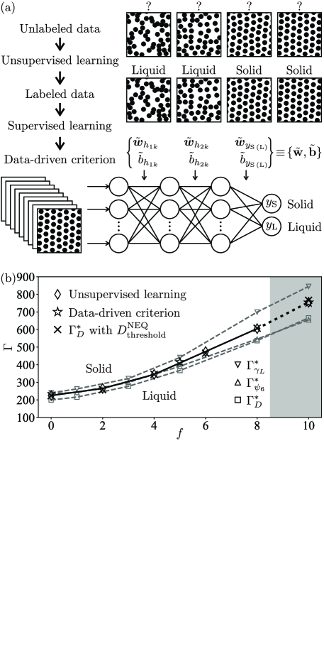
In this work, we address this question for 2D self-propelled colloidal particles with Yukawa-type interaction. To this end, we apply a hybrid machine learning approach that combines unsupervised learning with supervised learning to analyze a huge amount of the system’s configurations on an equal footing and establish an explicit data-driven criterion for identifying the solid-liquid transition of the system in the far from equilibrium parameter regime (cf. Fig. 1). More specifically, after generating $\sim\mathcal{O}(10^{6})$ spatial distributions of colloidal particles in the NEQ steady state [cf. the first row of Fig. 1(a)] via direct numerical simulations of the dynamical equation (1) of the system, these spatial distributions are analyzed by an unsupervised learning approach (van_Nieuwenburg_Nat_Phys_2017, ) that is realized by a fully connected neural network (NN) (Nielsen_Book_2015, ; Goodfellow_Book_2016, ). As a direct result, this gives an essentially unbiased (in the sense of no prior empirical assumptions being involved) criterion to classify the spatial distributions, according to which the solid-liquid transition boundary is extracted [cf. the solid curve in Fig. 1(b)]. Crucially, this also promotes the unlabeled data to the labeled data, which enables the direct supervised learning to concretize the criterion in the form of a set of NN-parameters that defines the NN [cf. the last row of Fig. 1(a)]. This thus establishes the explicit data-driven criterion that is able to identify the transition not only within, but also beyond the NEQ parameter regime where the supervised learning is directly performed [cf. the stars in Fig. 1(b)], indicating that it indeed captures the essential feature of the solid-liquid transition in the far from equilibrium parameter regime. Furthermore, by utilizing the so-called classification accuracy generated in the unsupervised learning process [cf. Eq.(2) and Fig. 2(b)], we establish a generic data-driven evaluation function [cf. Eq. (3)], according to which the performance of different empirical criteria can be systematically evaluated and improved. The direct application of this evaluation function gives rise, in particular, to a new NEQ threshold value $D_{\mathrm{threshold}}^{\mathrm{NEQ}}$ for the long-time diffusion coefficient, based on which the predictions of the corresponding empirical criterion are greatly improved in the far from equilibrium parameter regime [cf. Fig. 3 and the “$\times$” marks in Fig. 1(b)]. Moreover, since the underlying machine learning techniques exploited in this work are completely general, we expect that these data-driven approaches can readily provide new physical insights into phase transitions in other complex systems where conventional empirical approaches face difficulties.

II Self-propelled colloidal particles and their 2D solid-liquid transition

Figure 1: (a) Schematic illustration of the hybrid machine learning approach. Spatial distributions of particles are first processed by the unsupervised learning with a fully connected NN, after which the unlabeled data are promoted to the labeled data. These labeled data are processed by the supervised learning to optimize the learnable parameter set of the NN and get the optimal set $\{\tilde{\mathbf{w}},\tilde{\mathbf{b}}\}$ that determines the data-driven criterion. (b) Solid-liquid transition points predicted by the direct unsupervised learning (marked by “$\diamondsuit$” and solid curve), the data-driven criterion (marked by stars at $f=5$ and $f=10$), and the generalized empirical criterion with the NEQ threshold $D_{\mathrm{threshold}}^{\mathrm{NEQ}}$ (marked by “$\times$”). For comparison, the transition points $\Gamma_{\psi_{6}}^{*}$, $\Gamma_{D}^{*}$, and $\Gamma_{\gamma_{L}}^{*}$ predicted by the conventional empirical criteria using $\psi_{6}$, $D$, and $\gamma_{L}$, respectively, are shown by the dashed curves (reprinted from Ref. (Lowen_PRL_2012, )). The data-driven criterion and the NEQ threshold $D_{\mathrm{threshold}}^{\mathrm{NEQ}}$ are obtained by “learning” the configurations of the system with $f=0,2,4,6,8$. Their predicted transition points match very well with the ones from the direct unsupervised learning, not only in the parameter regime $f\in[0,8]$ in which the data are directly accessible to them, but also in the parameter regime well beyond (the shaded area). See text for more details.

The system under study consists of $N$ self-propelled colloidal particles in a 2D space (Lowen_PRL_2012, ), whose dynamics is described by a set of overdamped Langevin-type equations with the explicit form,

$$\dot{\boldsymbol{r}}_{i}=-\nabla_{i}U+f\boldsymbol{e}_{i}+\boldsymbol{\xi}_{i}.$$ (1)

Here, $\boldsymbol{r}_{i}$ is the position of the $i$th particle, and $\boldsymbol{\xi}_{i}$ is the noise which models the stochastic interactions with the solvent molecules. The noise assumes zero mean and correlations $\langle\boldsymbol{\xi}_{i}(t)\boldsymbol{\xi}_{j}^{T}(t^{\prime})\rangle=2\delta_{ij}\boldsymbol{1}\delta(t-t^{\prime})$, where $\langle\cdot\rangle$ denotes an ensemble average over the distribution of noise and $\delta(t)$ is the Dirac delta function. $f$ is the strength of the force that propels each particle in the direction $\boldsymbol{e}_{i}\equiv(\cos\varphi_{i},\sin\varphi_{i})$, where $\langle\dot{\varphi}_{i}(t)\dot{\varphi}_{j}(t^{\prime})\rangle=2\Delta\delta_{ij}\delta(t-t^{\prime})$ with $\Delta$ being the so-called rotational diffusion coefficient. $U=\sum_{i<j}u(|\boldsymbol{r}_{i}-\boldsymbol{r}_{j}|)$ is the interaction potential between particles, with $u(r)$ assuming the form of the Yukawa potential, i.e., $u(r)=\Gamma\exp(-\lambda r)/r$. Here, $\lambda$ is the inverse screening length, $\Gamma\equiv V_{0}\sqrt{\rho}/k_{B}T$ is the effective interaction strength, with $V_{0}$, $\rho$, and $T$ being the bare potential strength, the density, and the temperature, respectively.

By using empirical criteria associated with the global bond-orientational order parameter $\psi_{6}$ (Steinhardt_PRB_1983, ; Hartmann_PRE_2005, ), the long-time diffusion coefficient $D$ (Lowen_PRL_1993, ; Lowen_PRE_1996, ), and the Lindemann-like parameter $\gamma_{L}$ (Zahn_PRL_2000, ), previous investigations have shown that for a fixed self-propelled force strength $f$, the system assumes two phases, namely, the solid phase at relatively large $\Gamma$ (corresponding to low temperature or high density) and the liquid phase at relatively small $\Gamma$ (corresponding to high temperature or low density) (Lowen_PRL_2012, ). However, it was also noted that the transition points predicted by these different empirical criteria for melting and freezing, although agree with each other in equilibrium ($f=0$), separate away when the system enters the NEQ parameter regime ($f>0$), essentially resulting in a lower and an upper bound for the solid phase region and the liquid one (footnote_1, ), respectively [cf. Ref. (Lowen_PRL_2012, ) or the upper and lower dashed curves in Fig. 1(b)].

Noticing that the direct reliance on the properties of certain physical quantities, namely, $\psi_{6}$, $D$, and $\gamma_{L}$, actually makes the empirical criteria utilize only certain parts of the available information of the system, it is intriguing to expect that a data-driven criterion that directly makes full use of the available information of the system would be able to identify the solid-liquid transition in both equilibrium and NEQ. Indeed, as we shall see in the following, such an explicit data-driven criterion can be established by directly analyzing a huge amount of the system’s configurations on an equal footing. Moreover, a data-driven evaluation function can also be established, according to which the performance of different empirical criteria can be systematically evaluated and improved.

III Data-driven criterion for the solid-liquid transition via hybrid machine learning approach

Figure 2: (a) Schematic illustration of the confusing labels involved in the unsupervised learning approach “learning by confusion”. The images with their corresponding $\Gamma$ satisfying $\Gamma^{*\prime}(f)<\Gamma<\Gamma^{*}(f)$ are in the liquid phase but labeled as “solid”, which confuses the NN in establishing the classification criterion. (b) Solid-liquid transition points identified by the NN trained via unsupervised learning. For each self-propelled force strength $f$, three independent data sets, denoted by “A”, “B”, and “C”, are used in the unsupervised learning process, and the classification accuracy $P(\Gamma^{*\prime}(f))$ for each independent data set reaches the same nontrivial maximum that corresponds to the solid-liquid transition point. The predicted transition points are $\Gamma^{*}(0)=225\pm 5$, $\Gamma^{*}(2)=265\pm 5$, $\Gamma^{*}(4)=345\pm 5$, $\Gamma^{*}(6)=475\pm 5$, and $\Gamma^{*}(8)=605\pm 5$. See text for more details.

The data-driven criterion is based on directly analyzing a huge amount of the system’s configurations, i.e., spatial distributions of particles, which are generated by direct numerical simulations of the dynamical equation (1) of the system in different parameter regimes. Here, we focus on the case with $N=1936$, $\Delta=3.5$, $\lambda=3.5$, $\rho=1$, and all the numerical simulations of Eq. (1) are performed in a 2D rectangular space with aspect ratio $2/\sqrt{3}$ and periodic boundary condition imposed according to the minimum-image convention (Rapaport_art_of_MDS_CUP_2004, ). In total, we generate $\sim\mathcal{O}(10^{6})$ spatial distributions of self-propelled colloidal particles in the steady state that correspond to different sets of effective interaction strength $\Gamma$ and self-propelled force strength $f$. These 2D distributions are then directly transformed into images, forming the whole data set which is directly processed by the NN that conducts the hybrid machine learning (cf. Fig. 1) as we shall now discuss.

The hybrid machine learning starts with the unsupervised learning performed by employing the so-called “learning by confusion” approach (van_Nieuwenburg_Nat_Phys_2017, ) that is realized by a fully connected NN [cf. Refs. (Nielsen_Book_2015, ; Goodfellow_Book_2016, ) and the last row of Fig. 1(a)]. Here, we notice that although intermediate phases can appear from time to time in various complex systems (Glotzer_PRX_2017, ; Guerra_Nature_2018, ; Digregorio_PRL_2018, ; Cugliandolo_PRL_2017, ; Komatsu_PRX_2015, ; Ning_Xu_PRL_2016, ; Ciamarra_PRL_2020, ; Krauth_Nat_Commun_2018, ; Buttinoni_JPHYS_CM_2021, ), for instance, in a related system with a relatively softer interaction potential (inverse-power-law repulsion), the intermediate hexatic phase was indeed identified in a quite narrow stripe region in the phase diagram (Krauth_Nat_Commun_2018, ), previous investigations have not resolve a possible intermediate phase for the finite-size system under study in this work (Lowen_PRL_2012, ) (see also Appendix F). Therefore, we use a relatively simple binary classification approach, i.e., “learning by confusion,” to identify the possible solid-liquid transition, instead of resorting to multiclass classification approaches, for instance, the one presented in Appendix F. This “learning by confusion” approach is an unsupervised learning approach in the sense that the existence of possible transitions is not assumed (van_Nieuwenburg_Nat_Phys_2017, ) but determined by itself via monitoring the contrast between good and bad recognition performance when “confusing labels” are deliberately attached to the images in the data set (cf. Fig. 2), despite being limited to investigate the cases where maximally two possible phases exist in the parameter regimes of interests. Moreover, since it is based on NN, a wide range of well-established powerful NN architectures can be employed in its realization (see Appendix E for a realization using a convolutional NN).

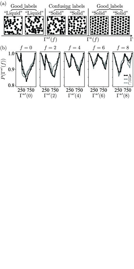
To implement the “learning by confusion” approach, images are labeled as “liquid” (“solid”) if their corresponding $\Gamma<\Gamma^{*\prime}(f)$ ($\Gamma>\Gamma^{*\prime}(f)$) by imposing a testing binary classification rule associated with a proposed critical value $\Gamma^{*\prime}(f)$ for the images corresponding to the same fixed self-propelled force strength $f$. This way of labeling generally confuses the NN when the proposed critical value $\Gamma^{*\prime}(f)$ is not equal to the physical critical value $\Gamma^{*}(f)$. For instance, if $\Gamma^{*\prime}(f)<\Gamma^{*}(f)$, the images with their corresponding $\Gamma$ satisfying $\Gamma^{*\prime}(f)<\Gamma<\Gamma^{*}(f)$ are in the liquid phase but labeled as “solid” [cf. Fig. 2(a)]. For a generic proposed value $\Gamma^{*\prime}(f)$, we train the NN and then test its classification accuracy,

$$P(\Gamma^{*\prime}(f))\equiv\frac{\mathcal{M}_{f}^{\textrm{``correct''}}(\Gamma^{*\prime}(f))}{\mathcal{M}_{f}^{\textrm{test}}},$$ (2)

with new testing images that have not been “seen” by the NN in the training process (see Appendix B for details). Here, $\mathcal{M}_{f}^{\textrm{test}}$ is the total number of the testing images and $\mathcal{M}_{f}^{\textrm{``correct''}}(\Gamma^{*\prime}(f))$ is the number of images that are classified “correctly” according to the proposed labels determined by $\Gamma^{*\prime}(f)$. Noticing that the closer $\Gamma^{*\prime}(f)$ is to the solid-liquid transition point $\Gamma^{*}(f)$, the fewer confusing labels exist, hence leading to the relatively higher accuracy, the classification accuracy $P(\Gamma^{*\prime}(f))$ should therefore assume a nontrivial maximum when $\Gamma^{*\prime}(f)$ matches $\Gamma^{*}(f)$.

As we can see from Fig. 2(b), where the unsupervised learning is performed separately for the data sets with corresponding $f=0,2,4,6,8$, the classification accuracy $P(\Gamma^{*\prime}(f))$ assumes a nontrivial maximum for each $f$, from which one can directly read out the corresponding transition point $\Gamma^{*}(f)$. The solid-liquid transition boundary formed by these transition points is shown in the phase diagram Fig. 1(b), where we can see that it locates exactly between the lower bound of the solid region set by $\Gamma_{\gamma_{L}}^{*}$ and the upper bound of the liquid region set by $\Gamma_{D}^{*}$, clearly corroborating the predictions from these conventional dynamical criteria (Lowen_PRL_2012, ) and suggesting there exists an underlying criterion that can capture the feature for distinguishing the solid from the liquid phase in the far from equilibrium parameter regime. This thus motivates us to extract the explicit form of this underlying criterion revealed by the unsupervised learning.

To achieve this goal, we first notice that the explicit form of the criterion can be generally regarded as a map from the space of the system’s configurations to two “confidence” values, say, $y_{\textrm{S}}$ and $y_{\textrm{L}}$ that hold the meaning of how likely a given configuration is a configuration of the solid and the liquid phase, respectively, i.e., a well-trained NN that takes the system’s configurations as input and outputs the correct confidence values [cf. the last row of Fig. 1(a)]. Crucially, according to the solid-liquid transition boundary predicted by the unsupervised learning, all available images with corresponding $f=0,2,4,6,8$, can be properly labeled now, thus promoting the original unlabeled data set to the labeled one. With the labeled data, the supervised learning realized by a fully connected NN with the learnable parameter set $\left\{\mathbf{w},\mathbf{b}\right\}$ can be directly performed and finally gives rise to the optimal learnable parameter set $\{\tilde{\mathbf{w}},\tilde{\mathbf{b}}\}$ that completely determines the well-trained NN (see Appendix A for details), i.e., the explicit data-driven criterion.

From Fig. 1(b) we can see that the prediction on the solid-liquid transition points from this data-driven criterion (see Appendix C for details) matches very well with the one from the direct unsupervised learning. In particular, for the transition point at $f=10$, it is located way beyond the parameter regime $f\in[0,8]$ in which the data are directly provided to the NN to be learned, clearly manifesting that this explicit data-driven criterion indeed captures the generic feature that distinguishes the solid from the liquid phase in the far from equilibrium parameter regime. Moreover, noticing that essentially only a lower bound for the solid phase region and an upper bound for the liquid phase region were identified by the conventional empirical approaches (Lowen_PRL_2012, ), the data-driven approach thus establishes the solid-liquid transition boundary in both the equilibrium and NEQ regimes for this system for the first time.

IV Data-driven evaluation function for empirical criteria

Figure 3: (a) $\Gamma$-dependence of the long-time diffusion coefficient $D$ of the system at different self-propelled force strengths $f=0,2,4,6,8$. The upper and the lower horizontal dashed lines correspond to the equilibrium threshold $D_{\mathrm{threshold}}^{\mathrm{EQ}}=0.086$ and the NEQ one $D_{\mathrm{threshold}}^{\mathrm{NEQ}}=0.025$ obtained by optimizing $\mathcal{P}_{D_{\mathrm{threshold}}}$, respectively. The crossings marked by “$\times$” of each horizontal dashed line with the $D(\Gamma)$ curves at different $f$ predict the corresponding transition points $\Gamma_{D_{\mathrm{threshold}}}^{*}(f)$. (b) Threshold value $D_{\mathrm{threshold}}$ dependence of the criterial classification accuracy $\mathcal{P}_{D_{\mathrm{threshold}}}$. The rightmost point corresponds to $D_{\mathrm{threshold}}=D_{\mathrm{threshold}}^{\mathrm{EQ}}=0.086$, and the point with the highest $\mathcal{P}_{D_{\mathrm{threshold}}}$ corresponds to $D_{\mathrm{threshold}}^{\mathrm{NEQ}}=0.025$ which results in a generalized empirical criterion with improved performance in the NEQ scenario. See text for more details.

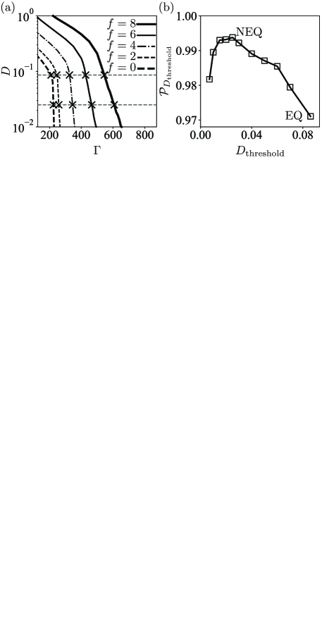
Besides the solid-liquid transition boundary in the far from equilibrium regime and its associated data-driven criterion, another class of physical insights that one can obtain by making full use of the available information of the system is a data-driven evaluation function, according to which the performance of different empirical criteria can be systematically evaluated and improved. From Eq. (2), we can see that for any given (empirical) criterion, denoted as $\mathcal{C}$, its performance can be naturally evaluated by the average classification accuracy of its predicted transition points at which a sufficient amount of the system’s configurations are available, i.e., a criterial classification accuracy denoted as $\mathcal{P}_{\mathcal{C}}$ with the explicit form,

$$\mathcal{P}_{\mathcal{C}}=\frac{1}{N_{f}}\sum_{i=1}^{N_{f}}P(\Gamma_{\mathcal{C}}^{*}(f_{i})),$$ (3)

where $\Gamma_{\mathcal{C}}^{*}(f_{i})$ is the transition point determined by $\mathcal{C}$ at the self-propelled force strength $f_{i}$ and $N_{f}$ is the total number of the transition points involved in the evaluation.

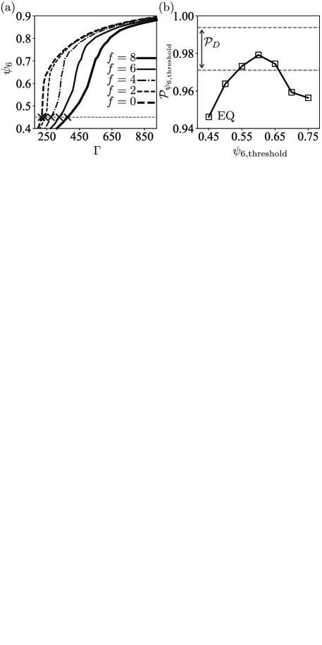
Taking the empirical criterion that uses an equilibrium threshold value $D_{\mathrm{threshold}}^{\mathrm{EQ}}=0.086$ for the long-time diffusion coefficient $D$ (Lowen_PRL_2012, ; Lowen_PRE_1996, ), for example, by utilizing the available data at $f=0,2,4,6,8$, its criterial classification accuracy $\mathcal{P}_{D_{\mathrm{threshold}}^{\mathrm{EQ}}}=\sum_{f=0,2,4,6,8}P(\Gamma_{D_{\mathrm{threshold}}^{\mathrm{EQ}}}^{*}(f))/5$ can be directly calculated, where $\Gamma_{D_{\mathrm{threshold}}^{\mathrm{EQ}}}^{*}(f)$ is the transition point at $f$ determined by this criterion [cf. upper row of “$\times$” in Fig. 3(a) and the rightmost point in Fig. 3(b)]. Noticing this criterion employs a threshold value motivated by the equilibrium behavior (Lowen_PRL_2012, ; Lowen_PRL_1993, ; Lowen_PRE_1996, ), hence leaves the space for further improvement if a general threshold value $D_{\mathrm{threshold}}$ is chosen [cf. the lower row of “$\times$” in Fig. 3(a)], we investigate the $D_{\mathrm{threshold}}$ dependence of the corresponding criterial classification accuracy $\mathcal{P}_{D_{\mathrm{threshold}}}$. From Fig. 3(b) we notice that at a smaller threshold than the equilibrium one, $\mathcal{P}_{D_{\mathrm{threshold}}}$ reaches the highest value, directly indicating that the corresponding criterion using this NEQ threshold, denoted as $D_{\mathrm{threshold}}^{\mathrm{NEQ}}$, assumes the best performance in the NEQ parameter regime $f\in[0,8]$. Indeed, the transition points predicted by this generalized empirical criterion are surprisingly close to the ones obtained by the direct unsupervised learning [cf. Fig. 1(b)]. More remarkably, although $D_{\mathrm{threshold}}^{\mathrm{NEQ}}$ is determined within the NEQ parameter regime $f\in[0,8]$, its predictive power extends well beyond, as manifested by its prediction of the transition point at $f=10$ which is still very close to the one via the direct unsupervised learning [cf. the shaded area in Fig. 1(b)]. This thus suggests that after generalizing this criterion (Lowen_PRL_2012, ; Lowen_PRL_1993, ; Lowen_PRE_1996, ) with a smaller NEQ threshold, it can identify the solid-liquid transition in both equilibrium and NEQ quite precisely, which is a clear improvement over the conventional empirical criterion, made by utilizing the data-driven evaluation function developed in this work. In fact, the improvement is also consistent with the natural expectation that, due to the fact that active systems in NEQ are more difficult to crystallize, the threshold value for the general NEQ scenario is supposed to be smaller than the one for the equilibrium case.

Moreover, we also perform a similar investigation on the empirical criterion based on the threshold value of the global bond-orientational order parameter $\psi_{6}$ (Lowen_PRL_2012, ) (see Appendix D for details) and find this criterion assumes relatively poor performance in general. Noticing that being a static structure criterion by construction as well, the data-driven criterion can indeed extract the solid-liquid transition boundary in both equilibrium and NEQ, this thus manifests that it is possible to develop a better static structure order parameter than $\psi_{6}$. Comparing the data-driven criterion and the global bond-orientational order parameter $\psi_{6}$, an obvious difference is that the former directly makes full use of the available information of the system while the latter essentially only utilizes information from groups consisting of the six nearest neighboring particles (Lowen_PRL_2012, ; Steinhardt_PRB_1983, ; Hartmann_PRE_2005, ). Therefore, one may expect that a more delicate static structure criterion with, for instance, structural defects such as dislocations, disclinations, etc., taken into account could improve the performance. Although constructing a better structural order parameter is beyond the scope of the current work, its performance can still be straightforwardly evaluated via the criterial classification accuracy $\mathcal{P}_{\mathcal{C}}$ established in this work. More generally, the data-driven evaluation function in fact offers a new type of generic tool to access crucial insights into the performance of existing (empirical) criteria and, in particular, facilitates the search for better criteria or order parameters associated with various phase transitions in complex systems.

V Conclusion and outlook

By directly analyzing over one million of the system’s configurations on an equal footing via data-driven approaches, new physical insights into the solid-liquid transition of the system in the far from equilibrium parameter regime are gained: An explicit data-driven criterion together with its predicted solid-liquid transition boundary is established via the hybrid machine learning approach that combines unsupervised learning with supervised learning. Furthermore, the data-driven criterial classification accuracy is established as a systematic way to evaluate and improve the empirical criteria, via which, in particular, a generalized conventional empirical criterion with a new NEQ long-time diffusion coefficient threshold is found and assumes a much enhanced performance in NEQ. These data-driven approaches open up a wide range of intriguing possibilities for further investigations to provide new physical insights into phase transitions in complex systems such as amorphous glass-formers (Biroli_Nat_Phys_2008, ; Albert_Science_2016, ) where conventional empirical approaches face difficulties.

Appendix A NN’s CONFIDENCE VALUES DETERMINED BY THE LEARNABLE PARAMETER SET

In this work, each sample of the data set is an image of $K_{0}=3\times 224\times 224$ pixels which can be directly analyzed by a wide range of standard NNs. In practice, this makes the test of robustness of the physical results obtained by the machine learning approach in this work against different NN architectures relatively convenient. Here, we choose the employed fully connected NN (Nielsen_Book_2015, ; Goodfellow_Book_2016, ) to consist of an input layer $\boldsymbol{x}\equiv(x_{1},x_{2},\cdots x_{k},\cdots,x_{K_{0}})^{T}$ with $K_{0}$ neurons, two fully connected hidden layers $\boldsymbol{h}_{1}\equiv(h_{11},h_{12},\cdots h_{1k},\cdots,h_{1K_{1}})^{T}$ and $\boldsymbol{h}_{2}\equiv(h_{21},h_{22},\cdots,h_{2k},\cdots h_{2K_{2}})^{T}$ with $K_{1}=K_{2}=2\times 10^{3}$ neurons, and an output layer with $2$ neurons $y_{\textrm{S}}$ and $y_{\textrm{L}}$. When a sample of our data, i.e., an image $I$ of the self-propelled colloidal particles’ spatial distribution, is fed to the fully connected NN, each neuron $x_{k}$ in the input layer $\boldsymbol{x}$ collects a single raw pixel of $I$ and delivers its value to the next layer. Each neuron $h_{1k}$ in the next layer, namely, the first hidden layer $\boldsymbol{h}_{1}$, receives $\boldsymbol{x}$ and takes the value $h_{1k}=\textrm{ReLU}(\boldsymbol{w}_{h_{1k}}^{T}\boldsymbol{x}+b_{h_{1k}})\equiv\max(0,\boldsymbol{w}_{h_{1k}}^{T}\boldsymbol{x}+b_{h_{1k}})$, where the rectified linear unit (ReLU) is a nonlinear activation function (Nielsen_Book_2015, ; Goodfellow_Book_2016, ). Similarly, each neuron $h_{2k}$ in the second hidden layer $\boldsymbol{h}_{2}$ takes the value $h_{2k}=\textrm{ReLU}(\boldsymbol{w}_{h_{2k}}^{T}\boldsymbol{h}_{1}+b_{h_{2k}})$, and, in the end,

$$y_{\textrm{S\,(L)}} =\textrm{Sigmoid}(\boldsymbol{w}_{y_{\textrm{S\,(L)}}}^{T}\boldsymbol{h}_{2}+b_{y_{\textrm{S\,(L)}}})$$

$$\equiv(1+\exp(-(\boldsymbol{w}_{y_{\textrm{S\,(L)}}}^{T}\boldsymbol{h}_{2}+b_{y_{\textrm{S\,(L)}}})))^{-1}.$$ (4)

The sigmoid function is another nonlinear activation function (Nielsen_Book_2015, ; Goodfellow_Book_2016, ), whose return value is within $\left[0,1\right]$ and therefore can be regarded as the “confidence” value. These two confidence values $y_{\textrm{S}}$ and $y_{\textrm{L}}$ hold the meaning of how likely any given configuration is a configuration of the solid and the liquid phase, respectively, and the learnable parameter set $\left\{\mathbf{w},\mathbf{b}\right\}\equiv\left\{\boldsymbol{w}_{h_{1k}},\boldsymbol{w}_{h_{2k}},\boldsymbol{w}_{y_{\textrm{S\,(L)}}},b_{h_{1k}},b_{h_{2k}},b_{y_{\textrm{S\,(L)}}}\right\}$ completely determines the map that takes the system’s configurations as input and gives the confidence values $y_{\textrm{S}}$ and $y_{\textrm{L}}$ as output.

Figure 4: Solid-liquid transition points predicted by the data-driven criterion. The predicted transition points (marked by stars) are (a) $\Gamma^{*}(5)=415$ and (b) $\Gamma^{*}(10)=754$, which match very well with the predictions from the direct unsupervised learning. Here, the self-propelled force strength $f=5$ is within the parameter regime $f\in[0,8]$ where the supervised learning is directly performed, while $f=10$ is way beyond $f\in[0,8]$. See text for more details.

Appendix B TRAINING PROCESS OF NN: SUPERVISED LEARNING AND UNSUPERVISED LEARNING

Here, we briefly outline how to train the NN, i.e., to optimize the learnable parameter set $\left\{\mathbf{w},\mathbf{b}\right\}$ with respect to the labels. For more thorough discussions on the machine learning techniques involved in the training process, we refer the reader to Refs. (Nielsen_Book_2015, ; Goodfellow_Book_2016, ).

To train the NN, one shall first label the data, where a label $\tilde{\boldsymbol{y}}=(\tilde{y}_{\textrm{S}},\tilde{y}_{\textrm{L}})^{T}$ is a suggestion of the expected $y_{\textrm{S}}$ and $y_{\textrm{L}}$. For instance, while labeling an image $I$ as “liquid”, we suggest that $I$ is $100\%$ likely to be a configuration of the liquid phase, namely, $\tilde{\boldsymbol{y}}=(0,1)^{T}$. In both the supervised learning process and the unsupervised learning process in this work, every sample of data used for training has a label. The major difference between these two learning process is whether the labels are physical. More specifically, labels in the supervised learning process are always expected to be physically correct, while labels in the unsupervised learning process are not always the case. After the labeling, the error of the confidence values compared to $\tilde{\boldsymbol{y}}$ can be quantified by the cross-entropy cost function $S=-(\tilde{y}_{\textrm{S}}\ln y_{\textrm{S}}+\tilde{y}_{\textrm{L}}\ln y_{\textrm{L}})$ (Nielsen_Book_2015, ; Goodfellow_Book_2016, ). Whenever the NN is “trained” in this work, $\left\{\mathbf{w},\mathbf{b}\right\}$ is optimized by minimizing the cost function $S$ traversing the training samples for $10$ epochs using the Adam method (Kingma_arXiv_2014, ) with the learning rate $1\times 10^{-3}$.

Figure 5: (a) $\Gamma$-dependence of the global bond-orientational order parameter $\psi_{6}$ of the system at different self-propelled force strengths $f=0,2,4,6,8$. The horizontal dashed line corresponds to the equilibrium threshold $\psi_{6\textrm{,threshold}}^{\textrm{EQ}}=0.45$. The crossings marked by “$\times$” of the horizontal dashed line with the $D(\Gamma)$ curves at different $f$ predict the corresponding transition points $\Gamma_{\psi_{6}}^{*}(f)$. (b) Threshold value $\psi_{6\textrm{,threshold}}$ dependence of the criterial classification accuracy $\mathcal{P}_{\psi_{6\textrm{,threshold}}}$. The leftmost point corresponds to $\psi_{6\textrm{,threshold}}=\psi_{6\textrm{,threshold}}^{\textrm{EQ}}=0.45$, and the point with the highest $\mathcal{P}_{\psi_{6\textrm{,threshold}}}$ corresponds to $\psi_{6\textrm{,threshold}}=0.6$ which is a general threshold value for $\psi_{6}$ in the NEQ scenario. For comparison, the highest and the lowest criterial classification accuracy associated with the long-time diffusion coefficient $D$, i.e., $\mathcal{P}_{D_{\mathrm{threshold}}^{\mathrm{NEQ}}}$ and $\mathcal{P}_{D_{\mathrm{threshold}}^{\mathrm{EQ}}}$, are shown by the upper and the lower horizontal dashed lines, respectively. See text for more details.

Appendix C TRANSITION POINTS PREDICTED BY THE DATA-DRIVEN CRITERION

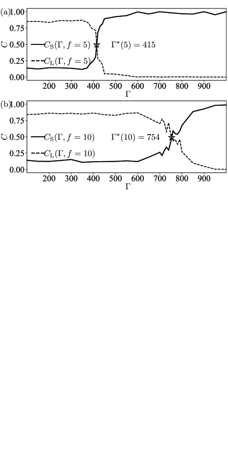
The data-driven criterion which captures the generic feature that distinguishes the solid from the liquid phase is expected to give equal confidence values $y_{\textrm{S}}$ and $y_{\textrm{L}}$ at the solid-liquid transition point, since the system can be either in the solid phase or the liquid phase. Therefore, after the supervised learning process with all the properly labeled data at $f=0,2,4,6,8$ in three independent data sets “A,” “B,” and “C,” the solid-liquid transition point for a fixed self-propelled force strength $f$ can be predicted by calculating the average classification confidence values (Melko_Nat_Phys_2017, ), whose explicit form reads $C_{\textrm{S\,(L)}}(\Gamma,f)=\sum_{n=1}^{\mathcal{N}_{\Gamma,f}}y_{\textrm{S\,(L)}}(I_{\Gamma,f;n})/\mathcal{N}_{\Gamma,f}$, where $I_{\Gamma,f;n}$ is the $n$th testing sample with its corresponding effective interaction strength being $\Gamma$ and $\mathcal{N}_{\Gamma,f}$ is the total number of these samples. Here, the intersection points of the $\Gamma$-dependence curves of $C_{\textrm{S}}$ and $C_{\textrm{L}}$ in Fig. 4 indicate $\Gamma^{*}(5)=415$ and $\Gamma^{*}(10)=754$, respectively, which match very well with the predictions from the direct unsupervised learning.

Moreover, as a piece of technical information, we provide here more details concerning the data set used in this work. For each different value of $(\Gamma,f)$, there are $7.2\times 10^{3}$ samples generated in the direct numerical simulations of the dynamical equation (1). The spacing for different $f$ is kept the same with $f=0,2,4,5,6,8,10$. In the expected deep solid and deep liquid regions, the spacing $\Delta\Gamma$ between different $\Gamma$ assumes a relatively larger value $\Delta\Gamma=50$, with $\Gamma=50,100,\ldots,1000$. While in the rest of the parameter region $\Delta\Gamma=10$, with $\Gamma=210,220,\ldots,290$ for $f=0$ and $f=2$; $\Gamma=310,320,\ldots,390$ for $f=4$; $\Gamma=360,370,\ldots,440$ for $f=5$; $\Gamma=410,420,\ldots,490$ for $f=6$; $\Gamma=560,570,\ldots,640$ for $f=8$; $\Gamma=710,720,\ldots,790$ for $f=10$.

Figure 6: (a) Solid-liquid transition point at self-propelled force strength $f=4$ identified by the CNN trained via the “learning by confusion” unsupervised learning, with a larger data set that is organized differently from the data set that corresponds to Fig. 2(b). For different particle number $N$ at constant global density $\rho=1$, the CNN’s classification accuracy $P(\Gamma^{*\prime}(f))$ reaches the same nontrivial maximum $\Gamma^{*}(4)=345\pm 5$ as the one obtained by the fully connected NN. This suggests the finite-size effects on the phase transition points are quite small at the system size mainly employed in this work (i.e., $N=1936$ and $\rho=1$). (b) Typical features implied in the weight map of the well-trained CNN’s first three convolutional layers concerning a sample of the solid phase with $\Gamma=1000$ at $f=4$, where the lighter color corresponds to the higher level of excitation. The weight map of the first convolutional layer (left panel) manifests a clear periodic structure, and for deeper layers (middle and right panels), it assumes a relatively homogeneous structure. (c) Analogous data to (b), but concerning a sample of the liquid phase with $\Gamma=50$ at $f=4$. The weight maps manifest a relatively disordered structure. (d) Solid-liquid transition points identified by the CNN trained via another machine learning approach that can detect the possible intermediate phases. Via calculating the signal $P_{\textrm{probe}}(\Gamma^{*\prime}(f))$ to probe the phase transition in the parameter region of interests, only one phase transition can be detected at each $f$ within a finite resolution $\Delta\Gamma=25$, indicating that this finite-size system assumes only two phases, which is consistent with previous investigations. And the predicted transition points agree well with the results in Fig. 2(b). See text for more details.

Appendix D CRITERIAL CLASSIFICATION ACCURACY AND THE NEQ THRESHOLD VALUE

For a given criterion $\mathcal{C}$, the transition point $\Gamma_{\mathcal{C}}^{*}(f_{i})$ at the self-propelled force strength $f_{i}$ is determined, and it corresponds to a binary classification rule associated with the proposed critical value $\Gamma^{*\prime}(f_{i})=\Gamma_{\mathcal{C}}^{*}(f_{i})$. Therefore, after the unsupervised learning process, the criterial classification accuracy $\mathcal{P}_{\mathcal{C}}=\sum_{i=1}^{N_{f}}P(\Gamma_{\mathcal{C}}^{*}(f_{i}))/N_{f}$ can be directly calculated according to the $\Gamma^{*\prime}(f_{i})$ dependence curves of the classification accuracy $P(\Gamma^{*\prime}(f_{i}))$. Concerning the empirical criterion associated with the long-time diffusion coefficient $D$, we monitor the criterial classification accuracy $\mathcal{P}_{D_{\mathrm{threshold}}}=\sum_{f=0,2,4,6,8}P(\Gamma_{D_{\mathrm{threshold}}}^{*}(f))/5$ by utilizing all the available data at $f=0,2,4,6,8$ in three independent data sets “A”, “B”, and “C”, and indeed find an optimal choice of a smaller NEQ threshold $D_{\textrm{threshold}}^{\textrm{NEQ}}=0.025$. However, for the empirical criterion associated with the global bond-orientational order parameter $\psi_{6}$, it assumes relatively poor performance in general. As we can see from Fig. 5(b), for this empirical criterion, the highest criterial classification accuracy $\mathcal{P}_{\psi_{6\textrm{,threshold}}}$ with a general threshold value $\psi_{6\textrm{,threshold}}=0.6$ for $\psi_{6}$ is just roughly around $\mathcal{P}_{D_{\mathrm{threshold}}^{\mathrm{EQ}}}$, and much lower than $\mathcal{P}_{D_{\mathrm{threshold}}^{\mathrm{NEQ}}}$ [cf. Figs. 3(b) and 5(b)].

Appendix E RESULTS BY EMPLOYING CONVOLUTIONAL NN

In the main text, we have established the data-driven criterion and the data-driven evaluation function by applying the hybrid machine learning approach realized by a fully connected NN. To address a few relevant technical aspects, here we present the physical results obtained by the same approach employing a NN with a different architecture, namely, a convolutional NN (CNN) called “AlexNet” (Krizhevsky_Adv_Neural_Inf_Process_Syst_2012, ) (with regularization implemented via “dropout”). As we shall see in the following, these results are the same as the ones obtained via the fully connected NN.

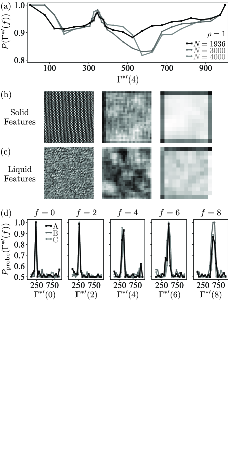
Here, we take the case with $f=4$ for instance. We perform the “learning by confusion” unsupervised learning using the CNN. Moreover, besides the NN with a different architecture employed to obtain the results shown in Fig. 6(a), the data set that corresponds to Fig. 6(a) is also organized differently from the one that corresponds to Fig. 2(b). For the former, all the samples generated by the same simulation are either used in the training, the validation, or the test (Nielsen_Book_2015, ; Goodfellow_Book_2016, ), while for the latter, the samples generated by the same simulation are divided into three parts for the training, the validation, and the test, respectively. In addition, for the former, the total number of samples in the data set is twice as large as the one for the later. As we can see from the black curve in Fig. 6(a), comparing with the middle column of Fig. 2(b), the CNN’s classification accuracy $P(\Gamma^{*\prime}(f))$ reaches the same nontrivial maximum as the one obtained by the fully connected NN. This manifests that the physical results obtained by the machine learning approach in this work are robust against these technical differences in its realization.

Moreover, we further study the influence of finite-size effects on the phase transition points. More specifically, we perform numerical calculations at different system sizes with the total particle number $N=1936,3000,4000$ and the global density $\rho=1$ keeping at constant. As we can see from Fig. 6(a), the predicted solid-liquid transition points (at $f=4$) of the system with larger sizes are numerically the same as the one of the system with $N=1936$ and $\rho=1$, i.e., $\Gamma^{*}(4)=345\pm 5$. This suggests that finite-size effects on the phase transition points are quite small at the system size ($N=1936$ and $\rho=1$) mainly employed in this work.

Finally, let us take the chance of utilizing the easily-accessed weight map (Nielsen_Book_2015, ; Goodfellow_Book_2016, ) of the CNN to visualize the feature used by the NN to perform the classification. In Figs. 6(b) and 6(c), we show typical features implied in the weight map (Nielsen_Book_2015, ; Goodfellow_Book_2016, ) of the well-trained CNN’s first three convolutional layers, where the lighter color corresponds to the higher level of excitation (Goodfellow_IEEE_T_PAMI_2013, ). The weight map of the first convolutional layer of the CNN manifests a clear periodic structure for the samples of the solid phase with $\Gamma=1000$ at $f=4$ [cf. the left panel of Fig. 6(b)], while a disordered structure for the ones of the liquid phase with $\Gamma=50$ at $f=4$ [cf. the left panel of Fig. 6(c)]. For deeper layers, the corresponding weight map assumes a relatively homogeneous structure for the solid phase [cf. middle and right panels of Fig. 6(b)], and a relatively disordered structure for the liquid phase [cf. middle and right panels of Fig. 6(c)]. From the general network structure of the CNN (Nielsen_Book_2015, ; Goodfellow_Book_2016, ), the behavior of the weight maps seems to suggest that the feature used by the CNN to classify samples is closely related to the spatial Fourier transformation of the system’s density distribution.

Appendix F INTERMEDIATE PHASE DETECTION

In the main text, the unsupervised part of the hybrid machine learning approach is limited to the cases where maximally two possible phases exist in the parameter regimes of interests. The major reason for choosing this approach comes from the fact that previous investigations have not resolved the possible (hexatic) intermediate phase in the system with a finite size (Lowen_PRL_2012, ).

To further check this point, here we use another machine learning approach developed recently (Guo_arXiv_2021b, ) that can detect the possible intermediate phases. In this new approach (Guo_arXiv_2021b, ), the signal to probe the phase transition, denoted as $P_{\textrm{probe}}(\Gamma^{*\prime}(f))$, is calculated for each narrow parameter interval $[\Gamma^{*\prime}(f)-\Delta\Gamma,\Gamma^{*\prime}(f)+\Delta\Gamma]$, with $\Gamma^{*\prime}(f)$ being the suspected phase transition point and $\Delta\Gamma$ being the resolution of the probe. Here, $P_{\textrm{probe}}(\Gamma^{*\prime}(f))$ is nothing but the classification accuracy of the NN concerning the data associated with the two boundaries of the corresponding interval, which indicates how likely there is a phase transition in the interval. As we can see from Fig. 6(d), via calculating $P_{\textrm{probe}}(\Gamma^{*\prime}(f))$ in the parameter region of interests, only one phase transition can be detected at each $f$ within a finite resolution $\Delta\Gamma=25$, indicating that this finite-size system assumes only two phases, which is consistent with previous investigations (Lowen_PRL_2012, ). We can also notice that the predicted transition points agree well with the results in Fig. 2(b) in the main text.

References

- (1) K. J. Strandburg, Rev. Mod. Phys. 60, 161 (1988).
- (2) J. M. Kosterlitz and D. J. Thouless, J. Phys. C 6, 1181 (1973).
- (3) B. I. Halperin and D. R. Nelson, Phys. Rev. Lett. 41, 121 (1978).
- (4) D. R. Nelson and B. I. Halperin, Phys. Rev. B 19, 2457 (1979).
- (5) A. P. Young, Phys. Rev. B 19, 1855 (1979).
- (6) E. P. Bernard and W. Krauth, Phys. Rev. Lett. 107, 155704 (2011).
- (7) S. C. Kapfer and W. Krauth, Phys. Rev. Lett. 114, 035702 (2015).
- (8) J. Russo and N. B. Wilding, Phys. Rev. Lett. 119, 115702 (2017).
- (9) J. A. Anderson, J. Antonaglia, J. A. Millan, M. Engel, and S. C. Glotzer, Phys. Rev. X 7, 021001 (2017).
- (10) R. E. Guerra, C. P. Kelleher, A. D. Hollingsworth, and P. M. Chaikin, Nature (London) 554, 346 (2018).
- (11) P. Digregorio, D. Levis, A. Suma, L. F. Cugliandolo, G. Gonnella, and I. Pagonabarraga, Phys. Rev. Lett. 121, 098003 (2018).
- (12) L. F. Cugliandolo, P. Digregorio, G. Gonnella, and A. Suma, Phys. Rev. Lett. 119, 268002 (2017).
- (13) Y. Komatsu and H. Tanaka, Phys. Rev. X 5, 031025 (2015).
- (14) M. Zu, J. Liu, H. Tong, and N. Xu, Phys. Rev. Lett. 117, 085702 (2016).
- (15) Y.-W. Li and M. P. Ciamarra, Phys. Rev. Lett. 124, 218002 (2020).
- (16) J. U. Klamser, S. C. Kapfer, and W. Krauth, Nat. Commun. 9, 5045 (2018).
- (17) L. Caprini, U. M. B. Marconi, C. Maggi, M. Paoluzzi, and A. Puglisi, Phys. Rev. Research 2, 023321 (2020).
- (18) J. Palacci, S. Sacanna, A. P. Steinberg, D. J. Pine, and P. M. Chaikin, Science 339, 936 (2013).
- (19) K. Dietrich, G. Volpe, M. N. Sulaiman, D. Renggli, I. Buttinoni, and L. Isa, Phys. Rev. Lett. 120, 268004 (2018).
- (20) T. B. Saw, W. Xi, B. Ladoux, and C. T. Lim, Adv. Mat. 30, e1802579 (2018).
- (21) J. Bialké, T. Speck, and H. Löwen, Phys. Rev. Lett. 108, 168301 (2012).
- (22) P. J. Steinhardt, D. R. Nelson, and M. Ronchetti, Phys. Rev. B 28, 784 (1983).
- (23) P. Hartmann, G. J. Kalman, Z. Donkó, and K. Kutasi, Phys. Rev. E 72, 026409 (2005).
- (24) H. Löwen, T. Palberg, and R. Simon, Phys. Rev. Lett. 70, 1557 (1993).
- (25) H. Löwen, Phys. Rev. E 53, R29 (1996).
- (26) K. Zahn and G. Maret, Phys. Rev. Lett. 85, 3656 (2000).
- (27) E. P. L. van Nieuwenburg, Y.-H. Liu, and S. D. Huber, Nat. Phys. 13, 435 (2017).
- (28) M. A. Nielsen, Neural Networks and Deep Learning (Determination Press, San Francisco, 2015).
- (29) I. Goodfellow, Y. Bengio, and A. Courville, Deep Learning (MIT Press, Cambridge, 2016).
- (30) The empirical criterion associated with the Lindemann-like parameter is a dynamical criterion for melting only, hence essentially determines a lower bound of for the solid phase region (Lowen_PRL_2012, ), above which the system is in a solid phase. While the one associated with the long-time diffusion coefficient is a dynamical criterion for freezing only, hence essentially determines an upper bound of for the liquid phase region (Lowen_PRL_2012, ), below which the system is in a liquid phase.
- (31) D. C. Rapaport, The Art of Molecular Dynamics Simulation, 2nd ed. (Cambridge University Press, Cambridge, 2004).
- (32) I. Buttinoni, G. Volpe, F. Kümmel, G. Volpe, and C. Bechinger, J. Phys. Condens. Matter 24, 284129 (2012).
- (33) G. Biroli, J.-P. Bouchaud, A. Cavagna, T. S. Grigera, and P. Verrocchio, Nat. Phys. 4, 771 (2008).
- (34) S. Albert, Th. Bauer, M. Michl, G. Biroli, J.-P. Bouchaud, A. Loidl, P. Lunkenheimer, R. Tourbot, C. Wiertel-Gasquet, and F. Ladieu, Science 352, 1308 (2016).
- (35) D. P. Kingma and J. L. Ba, in Proceedings of ICLR 2015 (International Conference on Learning Representations, San Diego, 2015).
- (36) J. Carrasquilla and R. G. Melko, Nat. Phys. 13, 431 (2017).
- (37) A. Krizhevsky, I. Sutskever, and G. E. Hinton, Commun. ACM 60, 84 (2017).
- (38) I. Goodfellow, A. Courville, and Y. Bengio, IEEE T. PAMI 35, 1902 (2013).
- (39) W. Guo, B. Ai, and L. He, arXiv:2106.16135.