Fiberized diamond-based vector magnetometers

Abstract

We present two fiberized vector magnetic-field sensors, based on nitrogen-vacancy (NV) centers in diamond. The sensors feature sub-nT/$\sqrt{\textrm{Hz}}$ magnetic sensitivity. We use commercially available components to construct sensors with a small sensor size, high photon collection, and minimal sensor-sample distance. Both sensors are located at the end of optical fibres with the sensor-head freely accessible and robust under movement. These features make them ideal for mapping magnetic fields with high sensitivity and spatial resolution ($\leq$ mm). As a demonstration we use one of the sensors to map the vector magnetic field inside the bore of a $\geq$ 100 mT Halbach array. The vector field sensing protocol translates microwave spectroscopy data addressing all diamonds axes and including double quantum transitions to a 3D magnetic field vector.

Introduction

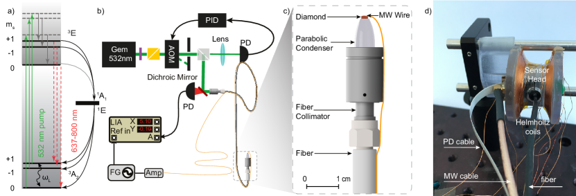
Figure 1: a) Relevant energy levels of the NV center. The states as well as their spin projection m_s are labeled. Solid green lines represent pump light, solid gray lines phononic de-excitation, dashed red lines represent PL, curved gray lines represent inter-system crossing. b) Experimental setup in Mainz (the experimental setup by Bosch can be found in Ref. Boscharxiv ). c) Schematic of the fiberized sensor head. d) Photograph of the fiberized sensor by Robert Bosch GmbH. The abbreviations used in the figure are; PD: Photo-diode, AOM: acousto-optic modulator, PID: proportional-integral-derivative controller, LIA: lock-in amplifier, FG: function generator, Amp: amplifier, MW: microwave.

Nitrogen-vacancy (NV) centers in diamond have attracted attention as magnetic field sensors with high spatial resolution Balasubramanian2008 ; Maze2008 ; Rittweger2009 and sensitivity Barry2016 ; Chatzidrosos . The range of their application includes, but is not limited to, single neuron-action potential detection Barry2016 , single protein spectroscopy Lovchinsky2016 , as well as in-vivo thermometry SingleNVThermometry . Advantages of NV-based magnetometers, compared to other magnetic field sensors, include their ability to operate in wide temperature and magnetic field ranges levelanticrossing . The ability to operate them also without the use of microwaves wickenbrock2016microwave ; levelanticrossing ; Zheng2020 , has recently enabled a variety of new applications in environments where microwaves (MW) would be detrimental Chatzi2019eddycurrent .

The NV consists of a substitutional nitrogen and an adjacent vacant carbon site. It can appear in different orientations along the crystallographic axes of the diamond lattice. This enables vector measurements of magnetic fields vectorClevenson . Vector magnetometry itself can be useful in magnetic navigation applications Cochrane , magnetic anomaly detection, current and position sensing, and the measurement of biological magnetic fields Barry2016 . Vector measurements near a background field of $\sim$ 100 mT, where the NV’s ground state level anti-crossing (GSLAC) occurs, are of particular interest Zheng2020 . Some of the challenges of vector measurements near the GSLAC field include the necessity to precisely align the NV and the bias magnetic field axes for optimum sensitivity of the microwave-free method levelanticrossing or the need to account for transversal field related nonlinearities of the NV gyromagnetic ratio when performing microwave spectroscopy.

One of the challenges NV magnetometers face is their low photon-collection efficiency. Approaches to increase the efficiency include, use of solid immersion lenses Hadden2010 ; Siyushev2010 ; Sage2012 , or employment of infrared absorption Dumeige2013 ; Budker1 ; Jensen2014 ; Chatzidrosos ; intraetalon . Photoluminescence (PL) for fiberized sensors is preferentially collected with the same fiber delivering the pump light but detected on the input side of the fiber fibersenso . Despite considerable effort, even modern sensors typically just feature a PL-to-pump-light ratio of about 0.1% fibersenso ; Barry2016 .

In this paper, we discuss the construction of two fiberized NV-based vector magnetic field sensors one constructed in Helmholtz Institute Mainz, referred to as Mainz sensor in the following and the other one is a sensor demonstrator of Robert Bosch GmbH, referred to as Bosch sensor in the following. They both achieve sub-nT$/\sqrt{\textrm{Hz}}$ magnetic sensitivity. The sensor constructed in Mainz achieved a sensitivity of 453 pT/$\sqrt{\textrm{Hz}}$, limited by intensity noise of the pump laser, with 11 pT/$\sqrt{\textrm{Hz}}$ photon-shot noise sensitivity and 0.5% PL-to-pump power ratio taking the fiber coupling efficiency into account. The sensor constructed by Bosch achieved a sensitivity of 344 pT/$\sqrt{\textrm{Hz}}$, which was approximately one order of magnitude larger than the expected photon-shot noise limited sensitivity Boscharxiv . The PL-to-pump power ratio was 0.3% taking the fiber-coupling efficiency into account. The components used for the construction of both sensors are commercially available. They allow for a small sensor size (11 $\times\,$40 mm² for Mainz and 15 $\times$ 25 mm² for Bosch) with maximized PL-to-pump-light ratio, as well as robustness to movement, which also makes the sensors portable. All of this makes the sensors ideal for mapping magnetic fields and measuring in regions that are not easily accessible. The magnetometers are constructed in such a way that they allow close proximity of the sensors to magnetic field sources, thus allowing for high spatial resolution when mapping magnetic fields. After demonstrating the sensitivity of the sensors and explaining the principles of vector magnetometry with NV centers, we used the Mainz sensor to perform spatially resolved optically detected magnetic resonance (ODMR) measurements covering an area of $20\times 30\,\text{mm}^{2}$ inside a Halbach-magnet array. The Halbach array itself provides a highly homogeneous magnetic field around 100 mT which makes it ideal for near-GSLAC magnetic field measurements and studies with NV centers. We present the analysis for the translation of the extracted frequency measurements into magnetic field. Details about the construction of the highly homogeneous Halbach array is subject of another publication Halbach .

Experimental Setup

The diamond sample used for the Mainz sensor is a 2.0 $\times$ 2.0 $\times$ 0.5 mm³ type Ib, (100)-cut, high-pressure high-temperature (HPHT) grown sample, purchased from Element Six. The initial [N] concentration of the sample was specified as $<$ 10 ppm. The sample was irradiated with 5 MeV electrons at a dose of $2\times 10^{19}\,\textrm{cm}^{-2}$ and then annealed at 700 ^∘C for 8 hours. The diamond sample used for the Bosch sensor is a $0.8\,\times\,0.8\,\times\,0.5\,\textrm{mm}^{3}$ (111)-cut, 99.97 % ¹²C enriched, HPHT grown diamond. The sample was irradiated with 2 MeV electrons at a dose of $2\,\times\,10^{18}\,\textrm{cm}^{-2}$ at room temperature and then annealed at 1000 ^∘C for 2 hours in vacuum. The [NV^-] concentration was determined by electron spin resonance to be 0.4 ppm Boscharxiv .

Figure 1 (a) shows the relevant energy levels of the negatively charged NV center, which we use for magnetometry. The ground and excited spin-triplet states of the NV are labeled ³A₂ and ³E, respectively [Fig. 1 (a)], the transition between them has a zero-phonon line at 637 nm, but can be exited by more energetic photons (of shorter wavelengths) due to phonon excitation in the diamond lattice. The lower and upper electronic singlet states are ¹E and ¹A₁, respectively. While optical transition rates are spin-independent, the probability of nonradiative intersystem crossing from ³E to the singlets is several times higher Dumeige2013 for $m_{s}=\pm 1$ than that for $m_{s}=0$. As a consequence, under continuous illumination with green pump light (532 nm), NV centers accumulate mostly in the ³A₂, $m_{s}=0$ ground state sublevel and in the metastable ¹E singlet state. For metrology applications, the spins in the ³A₂ ground state can be coherently manipulated with microwave fields.

Figure 1 (b) shows the experimental setup used for the measurements conducted in Mainz. To initialize the NV centers to the ground-triplet state, we use a 532 nm (green) laser (Laser Quantum, gem532). To reduce intensity noise from the laser source, the light intensity is stabilized using an acousto-optic modulator (AOM, ISOMET-1260C with an ISOMET 630C-350 driver) controlled through a proportional-integral-derivative controller (PID, SIM960), in a feedback loop. The green laser is then coupled into a 2 m long, high-power multi-mode fiber cable (Thorlabs, MHP365L02).

The MW to manipulate the NV spins are generated with a MW function generator (FG; SRS, SG394). They are amplified with a 16 W amplifier (Amp; Mini-Circuits, ZHL-16W-43+) and passed through a circulator (Mini-Circuits, CS-3.000) before they are applied to the NV centers using a mm-sized wire loop. The other side of the wire is directly connected to ground. The radius of the wire used for the wire loop is 50 $\mu$m. The wire is then attached to the optical fiber allowing the two parts to move together. For the magnetic resonance measurements presented in this paper, the MW frequency was scanned between 3800 MHz and 5000 MHz. Information on the experimental setup used to conduct the measurements with the Bosch sensor can be found in Ref Boscharxiv .

$f_{res}$	$f_{mod}$	$f_{depth}$	Detection limit
2880.4 MHz	3 kHz	100 kHz	3.7 $\pm$ 0.6 nT/$\sqrt{\textrm{Hz}}$
2894.3 MHz	2 kHz	100 kHz	3.1 $\pm$ 0.3 nT/$\sqrt{\textrm{Hz}}$
2873.5 MHz	5 kHz	100 kHz	2.7 $\pm$ 1.6 nT/$\sqrt{\textrm{Hz}}$

Table 1: Settings and detection limit for the three different NV axis used in the Bosch sensor.

A schematic of the Mainz fiberized magnetic field sensor head is shown in Fig. 1 (c). The diamond is glued to a parabolic condenser lens, which itself is glued onto a 11 mm focal length lens and attached to a fiber collimator (Thorlabs, F220SMA-532) to which the high-power multi-mode fiber (Thorlabs, MHP365L02) is connected. The MW wire loop is attached to the other side of the diamond to provide the rapidly oscillating magnetic fields required for this magnetic field detection scheme. The light is delivered to the diamond via the parabolic condenser, lens, collimator and the high-power fiber. The same components collect the spin-state-dependent red PL of the NV ensemble. On the other side of the fibre the PL is filtered using a longpass dichroic filter (Thorlabs, DMLP605) which is also used to couple the incoming green light into the fiber. After the dichroic filter residual reflected green light is removed by a notch filter (Thorlabs, NF533-17) and the PL is focused onto a photodiode (PD; Thorlabs, PDA36a2). The detected signal with the PD is connected to a a lock-in amplifier (LIA; SRS, SR830). With this setup we were able to achieve 0.5% PL-to-pump-light ratio, which is an order-of-magnitude improvement compared to other fiberized sensors fibersenso . A photograph of the Bosch sensor can be seen in Fig. 1 (d). The sensor head, containing a microwave resonator, a custom designed balanced photodetector, and the diamond, which was glued to the collimated output of a single-mode fiber, is located inside a custom designed Helmholtz coil. The Helmholtz coil was used to generate a magnetic bias field of 1.07 mT and the collimation of the laser beam was achieved with a gradient-index lens (GRIN). Further details on the setup used for the Bosch sensor can be found in Ref. Boscharxiv . The final sensor head, of the Mainz sensor, has a diameter of $\leq$ 11 mm and a height of 40 mm, in a configuration that allows for $\leq$ 300 $\mu$m average distance between sample and sensor. The 2 m long fiber with the attached MW wire and the fiberized sensor head for the Mainz sensor (shown in Fig. 1 (c)) can be moved independently of the other components. The footprint of the sensor head of the Bosch sensor was 15 $\times$25 mm². The smallest distance between the center of the diamond and the outer surface is roughly 2.4 mm, the sensor can move independently as well. To filter low-frequency systematic noise components, e.g. laser-power fluctuations, the MW-frequency $\omega_{L}$ is modulated and the detected PL is demodulated with the LIA. To produce the magnetic field maps presented here, the Mainz sensor assembly was mounted on a computer-controlled motorized 3D translation stage (Thorlabs, MTS25/M-Z8) in the center of the Halbach array (not shown in Fig. 1).

Magnetic field sensitivity

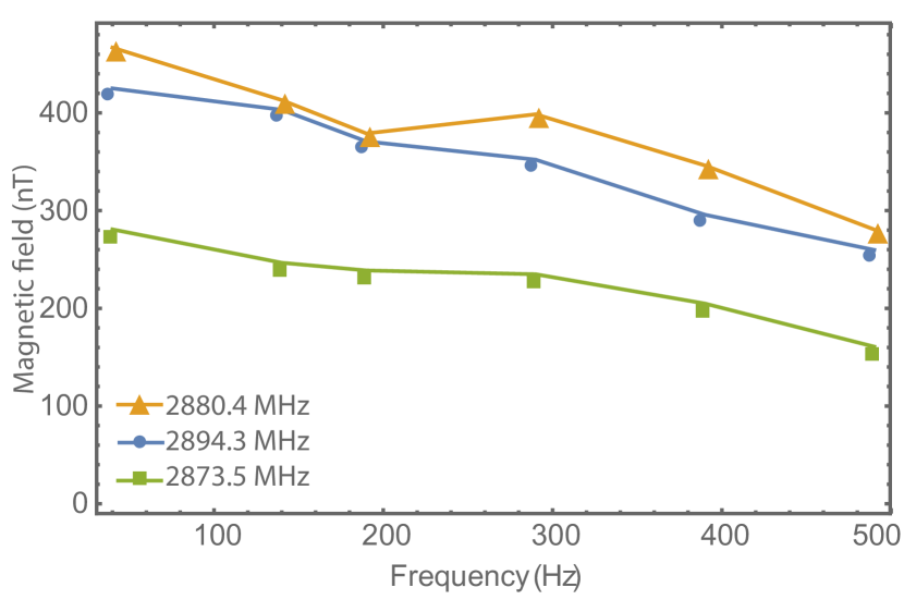
Figure 2: Amplitude of magnetic test signal, measured along three different NV axes with the Bosch sensor. An oscillating, external magnetic field of about 0.7 µT was applied to the sensor.

Figure 2 depicts the response of the Bosch sensor for three different NV axes upon application of an AC magnetic field with varying frequencies and a constant amplitude of 0.7 $\mu$T. The three axes see different effective amplitudes due to the different angles of the NV axes with respect to the magnetic field vector as expected. The sensor response slightly decreases with increasing frequency of the test field independent of the axis. This decrease might stem from the fact, that with increasing frequency, the excitation field becomes under-sampled meaning that the full reconstruction of the sinusoidal excitation field is not possible anymore leading to a decrease in measured amplitude.

To estimate the magnetic sensitivity of the two sensors we follow another method. When the MW field is resonant with the ground-state $m_{s}=0$ $\rightarrow$ $m_{s}=\pm 1$ transitions, population is transferred through the excited triplet state to the metastable singlet state, resulting in PL reduction. PL as a function of MW frequency is the ODMR signal. By focusing around a single of feature in this ODMR signal the sensitivity can be extracted. The magnetic resonance for the Mainz sensor features a 350 kHz linewidth and 1.6 % contrast. The best sensitivity of the Bosch sensor was achieved with a linewidth of $\approx$ 92 kHz and a contrast of 0.6 %. We modulate the MW frequency around a central frequency f_c, and record the first harmonic of the transmission signal with a LIA. This generates a demodulated signal, which together with the NV gyromagnetic ratio of $|^{\gamma}/_{2\pi}|\sim 28.024\,\rm{GHz}\,\rm{T}^{-1}$ can be used to translate PL fluctuations to effective magnetic field noise. The optimized parameters resulting in the best magnetic field sensitivity for the Mainz sensor were: a modulation frequency of f_mod = 13.6 kHz and modulation amplitude of f_amp = 260 kHz. The sensitivity of the Bosch sensor was optimized for 3 different NV axes as summarized in table 1.

Figure 3 shows the magnetic-field-noise spectrum of the sensors. The blue trace of Fig. 3 corresponds to magnetically sensitive data of the Mainz sensor, the orange to magnetically insensitive. The purple and green trace correspond to magnetically sensitive spectrum of the Bosch sensor outside and inside a magnetic shield, respectively, finally the red trace corresponds to the insensitive plot. The magnetically insensitive spectrum can be obtained if f_c is selected to be far from the ODMR features. The peak at 50 Hz is attributed to magnetic field from the power line in the lab. The average sensitivity in the 60-90 Hz area is 453 pT/$\sqrt{\textrm{Hz}}$ and 344 pT/$\sqrt{\textrm{Hz}}$ for the Mainz and Bosch sensors, respectively.

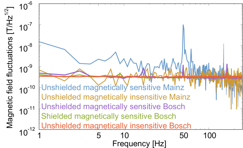
Figure 3: Magnetic field fluctuations measured with the fiberized NV magnetometers. The blue and orange traces depict magnetically sensitive and insensitive data of the Mainz sensor. The purple and green traces correspond to magnetically sensitive spectra of the Bosch sensor outside and inside a magnetic shield, finally, the red trace corresponds to unshielded magnetically insensitive data. The average sensitivity in the 60-90 Hz band is sub-nT/$\sqrt{\textrm{Hz}}$. The Bosch data are the result of 100 averages, while the Mainz data is from a single acquisition.

The noise traces for the Bosch sensor are based on continuous data series, that are recorded with a sampling rate of 1 kHz for 100 s. To calculated the amplitude spectral density (ASD), the data series was split in 100 consecutive intervals, each with a duration of 1 s. For each interval the ASD was calculated. The depicted is the average of the 100 ASDs.

Vector magnetic field sensing

Data Acquisition

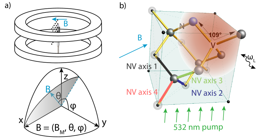
Figure 4: a) The orientation of the diamond sensor in the Halbach array. The orientation of the magnetic field is given in spherical coordinates with angle $\theta$ being the latitude angle with respect to the x-axis and $\phi$ the longitude. The main component of the magnetic field points along the x-axis. b) Illustration of the diamond lattice structure indicating the four different NV axes 1,2,3,4 and their relation to the applied magnetic field B. Microwaves (MW) with frequency $\omega_{L}/\left(2\pi\right)$ are applied to the sample.

As a demonstration of the robustness and portability of our sensors as well as the ability to produce highly resolved magnetic field maps, we select the Mainz sensor to characterize the homogeneity of a custom-made Halbach-array magnet constructed in the Mainz laboratory. The schematic of the magnet is shown in Fig. 4 (a) with more details found in Ref. Halbach . It is a double ring of permanent magnets arranged to generate a homogeneous magnetic field in its inner bore along the radius of the rings. The field outside the construction decays rapidly with distance. We performed ODMR measurements in a $30\times 20\,\text{mm}^{2}$ plane nearly perpendicular to the main magnetic field direction in the center of the Halbach array in steps of 1 mm and 1.5 mm in $z$ and $y$-direction, respectively. The experimental procedure to characterize this magnet involves reconstruction of the 3D magnetic field from these ODMR measurements, which we describe in the next part of this paper. The measurements confirmed the homogeneity of the magnetic field of the magnet to be consistent with Hall-probe and NMR measurements, but with a threefold improved field strength resolution, vector information of the magnetic field and sub-mm spatial information of these quantities. The orientation of the fiberized sensor in the Halbach magnet can be seen in Fig. 4 (a). The magnetic field is given in spherical coordinates with respect to the (100) axis of the diamond $\vec{B}=\left(B_{M},\theta,\phi\right)$. The angle between the magnetic field vector and the yz-plane is $\theta$, and $\phi$ is the angle between the projection of $\vec{B}$ in the yz-plane and the y-axis. The diamond sensor was oriented in the magnetic field such that different resonances were visible.

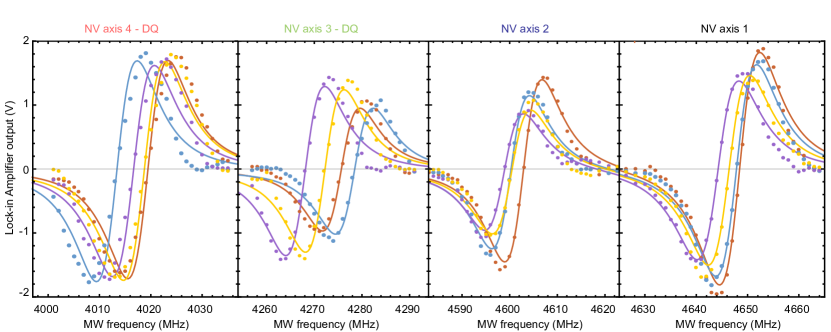
Figure 5: Example data traces of four optically detected resonances at different position near the center of the Halbach magnet. The resonances appear dispersive due to the use of a modulation technique. The resonances are fitted and their center frequencies are extracted. The four different plots correspond to different transitions indicated above the respective plot. The color of the traces indicate the positions at which the data was taken, as seen in Fig. 8.

For each position in the 30 $\times$20 mm² plane a scan of the applied MW frequency between 3800 MHz and 5000 MHz was performed in steps of 1 MHz. This range was limited by the bandwidth of the MW components. At each frequency we recorded the demodulated PL from the LIA x-output with a data acquisition system and stored each data set with its respective position. To speed up the acquisition and after determining that no features were left out, we just acquired in total 164 frequency values around the expected position of the resonances. In total a frequency scan to determine the four center frequencies lasted 46 s. This can be dramatically improved by for example applying a frequency lock on the four transitions, respectively.

Figure 5 shows an example of collected data in four different points of the scan. The points are noted in Fig. 8 (b) with different colors. The four different frequency regions correspond to different kind of transitions as noted above the figures. The FWHM linewidth of the observed features is ($11.48\pm 0.14$) MHz and therefore much larger than the one given above ($0.35\pm 0.02$) MHz for a small background field along one of the NV axis. This is due to the strong transverse field component but also caused intentional via MW power broadening. This simplified the lineshape by suppressing the hyperfine features in the spectrum and therefore the analysis routine. We additionally like to note, that the two first of the features are double quantum transitions (DQ), i.e. magnetic transitions from the $m_{s}=-1$ to the $m_{s}=+1$ state, normally forbidden, but allowed when transverse magnetic field components are present.

Overall the sensor was moved in steps of 1 mm and 1.5 mm in $z$ and $y$-direction, respectively, such that the whole area was covered. The resulting frequency maps of the chosen four resonances can be seen in Fig. 8 (a); they show structures corresponding to the strength of the longitudinal (along the NV axis) and transverse (perpendicular to the NV axis) component of the magnetic field for a given diamond lattice axis. The information contained in these plots is more than sufficient to reconstruct all three vector components of the magnetic field at the position of the sensor.

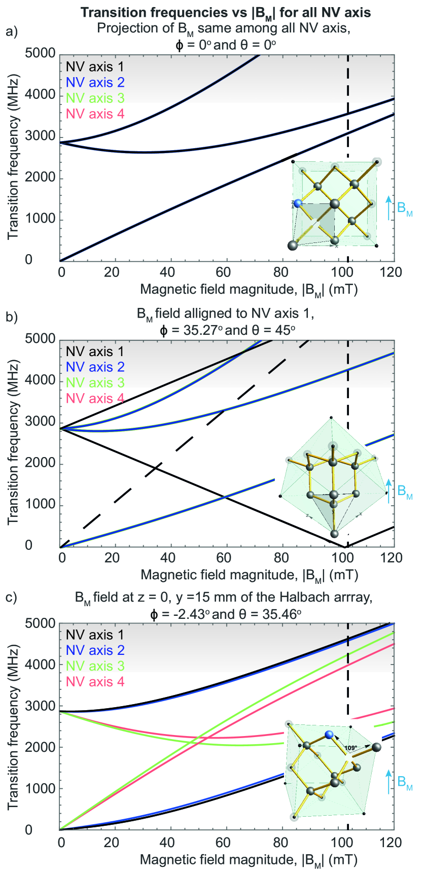
Figure 6: Transition frequencies as a function of $|B_{M}|$. The traces of the four different NV axes are depicted with colours consistent with those of Fig. 4. The gray area represents our scanning range, the vertical dashed line shows the mean field strength inside the Halbach magnet. a) For a magnetic field perpendicular to the (100) plane: all transitions overlap since the magnetic field projection is the same among all axes. b) For a magnetic field perpendicular to the (111) plane of a diamond: the magnetic field is aligned along NV axis 1, and the magnetic field projection is the same for the other three axes. The slanted dashed line for NV axis 1 corresponds to the frequency of the DQ transition which in this case due to the absence of transverse magnetic fields is not allowed. c) For a magnetic field configuration inside the Halbach magnet.

Frequency to vector field conversion

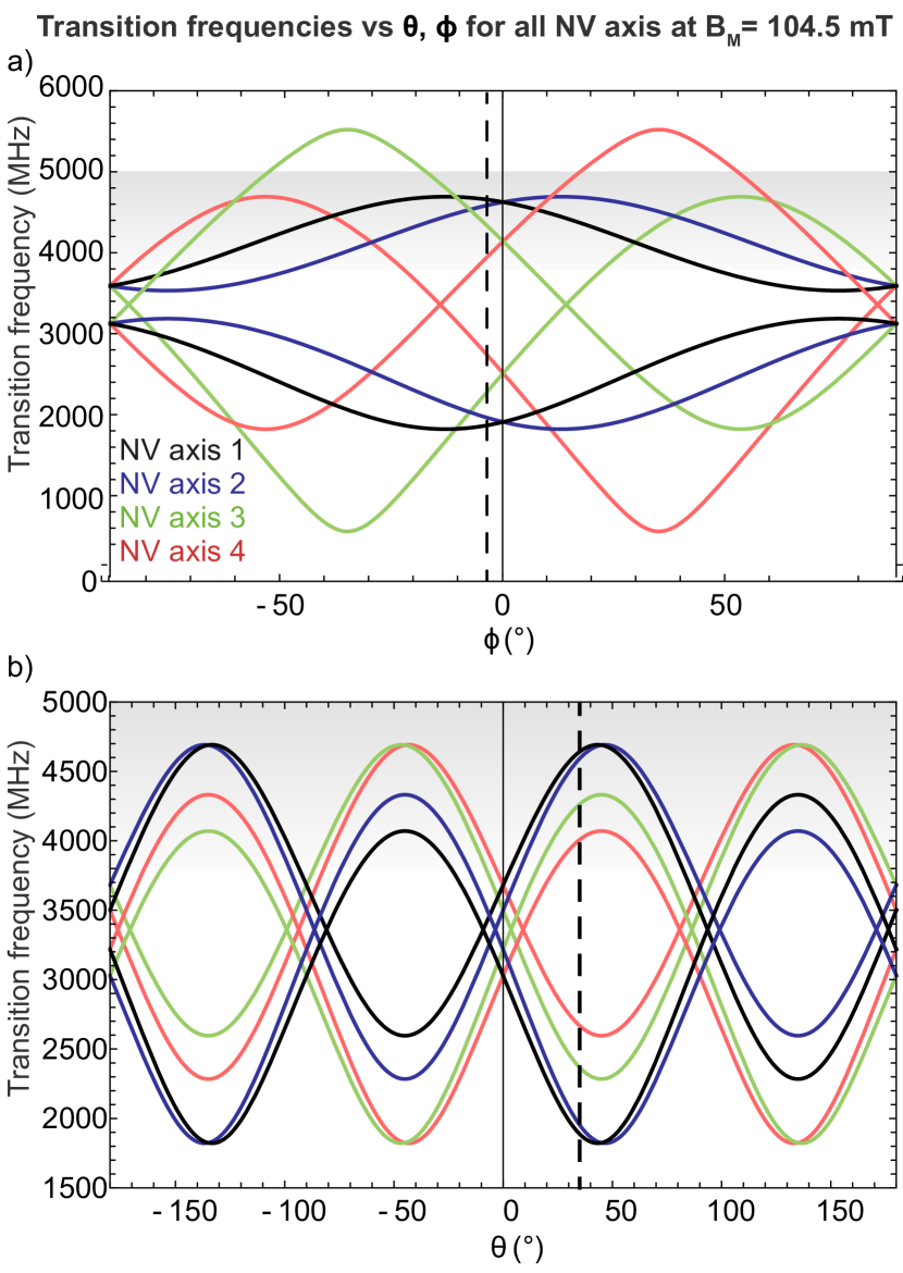
Figure 7: Simulated transition frequencies as a function of angles $\theta$ and $\phi$ for the average magnetic field magnitude $|B_{M}|=104.5$ mT inside the Halbach magnet. The gray area represents our frequency scan range, the vertical dashed line indicates the respective average angle of all the measurements. a) Transition frequencies as a function of angle $\theta$ for a fixed angle $\phi=-2.43^{\circ}$. b) Transition frequencies as a function of angle $\phi$ for a fixed angle $\theta=35.46^{\circ}$.

After acquiring MW frequency scans for different positions, the data were fitted with the sum of four derivatives of Lorentzians. The four center frequencies, four amplitudes and a combined linewidth were fit parameters, an example of the data and fits can be seen in Fig. 5. By matching these frequencies to the positions of the 3D translation stages we can make frequency maps as shown in Fig. 8 (a).

To proceed with the analysis and construction of the magnetic field maps we note that the four different features presented in Fig. 5 originate from the different NV orientations in the diamond crystal. The positions of these features are related to the alignment of the magnetic field to the NV axis, as well as its amplitude. If the magnetic field is along the NV axis (longitudinal) we observe the $m_{s}=0\rightarrow\,m_{s}=\pm 1$ transitions; if there is an additional magnetic field component orthogonal to the NV axis (transverse), transitions between the $m_{s}=-1$ and $m_{s}=+1$ are allowed. We call these double quantum (DQ) transitions. For a given magnetic field direction at the position of the sensor, both, the longitudinal and transverse components of the magnetic field are present. Due to mixing caused by the transverse magnetic field component, the NV gyromagnetic ratio depends on the background field strength.

As a result, to match the above frequencies to magnetic fields we create four vectors describing the NV axes. We use parameters $\beta$ to describe the angle between NV axis and magnetic field and $\Omega$ for the field strength. With these parameters we derive a formula which describes the transition frequencies of the spin states, from m_s = 0 to m_s = -1, as well as m_s = -1 to m_s = +1 Simon . Here, we neglect strain and electric field effects.

The frequency of the resonances depends on the magnitube of the magnetic field B_M, as well as the angles $\theta$ and $\phi$ of the diamond orientation with respect to the magnetic field. Figure 6 shows the resonance frequency dependence as a function of magnetic field magnitude for different fixed angles $\theta$ and $\phi$. Figures 6 (a,b) represent a magnetic field perpendicular to common diamond surface cuts, (100) plane for (a) and (111) plane for (b), (c) depicts a configuration inside our Halbach magnet. Figure 7 shows the dependence of the transition frequencies on the angles $\theta$ and $\phi$ for a magnetic field matching the mean magnitude inside the Halbach magnet. In Fig. 7 (a) $\phi$ = -2.43^∘ and $\theta$ is varied. In Fig.7 (b) $\theta$ = 35.46^∘ and $\phi$ is varied.

In both Fig. 6 and Fig. 7 the four different NV axes are depicted with colours matching those in Fig. 4. We observe that in Fig. 6 (a) all the transitions overlap, as the projection of the magnetic field is the same among all axes. In Fig. 6 (b) the magnetic field is aligned along the NV axis 1, and its projection is the same for the other three axes, which appear overlapped in the figure. The dashed line for NV axis 1 corresponds to the frequency of the DQ transition which in this case is not allowed, as there is no transverse field on NV axis 1. Figure 6 (c) represents a case we encounter while measuring the field inside our Halbach magnet. In Fig. 7, we note the symmetry between NV axes 1,2 and 3,4 which arises because of the crystallographic structure of the diamond. We can use the information of the above plots to translate the frequency into magnetic field.

After identifying the possible transition frequencies, we use a numerical method to translate the frequencies into magnetic field direction and strength. For this method we restrict the magnetic field strength values to within 10% of what the estimated magnetic field produced by our Halbach array is. Once the magnetic field is calculated for all the different frequencies we express it in polar coordinates. When the initial values for direction and magnitude of the field are approximately known, we find that the reconstruction is unique. We choose $B_{M}$ to describe the strength of the field, angle $\theta$ the latitude angle with respect to the x-axis and $\phi$ the longitude angle as shown in Fig. 4 (a). Finally, we make a list of these parameters and plot them as shown in Fig. 8 (b). In Fig. 8 (b) we included four different coloured circles to represent the positions at which data for Fig. 5 are taken. The measured averages of angles $\theta$ and $\phi$ in the central $10\times 5$ mm² (y-x) of the Halbach magnet are $\left(-2.433\pm 0.009\right)^{\circ}$ and $\left(35.764\pm 0.018\right)^{\circ}$, respectively, which is consistent with the orientation of the diamond lattice (cf. Fig. 4) relative to the coordinate system of the magnet.

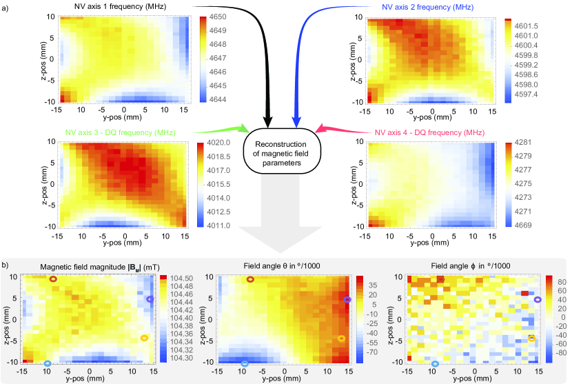
Figure 8: Figure adapted from Ref. Halbach . (a) Spatially resolved frequency maps of the individual resonances from Fig. 5 (a). (b) The data collected are used to reconstruct the vector magnetic field in spherical coordinates as defined in Fig. 4 (a), the four colored circles note the positions at which data for Fig. 5 are taken.

Conclusion and Outlook

We constructed two fiberized NV based magnetic field sensors. The sensors feature sub-nT/$\sqrt{\textrm{Hz}}$ magnetic field sensitivity with high PL-to-pump-light ratio. The components used to make the sensors are commercially available which makes their construction easy and reproducible. The design for the Mainz sensor was made in such a way as to allow free access to the front side of the diamond as well as for robustness, portability, and small size.

With one of the main challenges for NV magnetometry, especially fiberized, being the low photon-collection efficiency, which leads to poor photon-shot-noise limited sensitivity, the 0.5% PL-to-pump-light ratio collection efficiency, demonstrated in the Mainz sensor, can be used to achieve even higher sensitivity, if the effect of other noise sources is minimized. This ratio could also be further optimized by implementing side collection on the diamond Sage2012 ; 2019BarryNVReview , as well as highly reflective coatings on the opposite (front) side of the diamond. These features were not implemented in this sensor in order to keep all of its components commercial and easily accessible.

The access to the front side of the diamond allows for close proximity to magnetic field sources, which in turn leads to high spatial resolution. The proximity is currently limited to about 300 $\mu$m by MW wire on top of the diamond. It could be optimized further by using a thinner diamond sample, a sample with shallow implanted NV centers or a thinner MW wire such as, for example, a capton-tape printed circuit board, all depending on the intended application, as these changes influence the sensitivity of the sensor. Such optimization would be especially beneficial for measurements of dipole fields or measurements that require high spatial resolution.

The robustness and portability of the sensors also make them attractive for mapping larger areas, or on-the-move measurements of magnetic fields. These features combined with the small size of the sensors suggest a use for measuring in hard-to-access places or small areas where maneuverability of the sensor would be required, e.g. endoscopic measurements inside the human body.

As a demonstration of the Mainz sensor we measured the magnetic field of a custom-designed Halbach array. For these measurements, the small fiberized diamond sensor showed a mm-scale spatial resolution, angular resolution of the magnetic field vector extracted in the measurements were $9\times 10^{-3}$ degrees and $18\times 10^{-3}$ degrees for angles $\theta$ and $\phi$, respectively. We note here, that the corresponding displacement due to such a rotation of the diamond sensor (considering a $(0.5\times 0.5)$ mm² square cross section) could optically not be resolved.

References

- (1) F. M. Stürner, A. Brenneis, T. Buck, J. Kassel, R. Rölver, T. Fuchs, A. Savitsky, D. Suter, J. Grimmel, S. Hengesbach, M. Förtsch, K. Nakamura, H. Sumiya, S. Onoda, J. Isoya, and F. Jelezko, “Integrated and portable magnetometer based on nitrogen-vacancy ensembles in diamond,” arXiv:2012.01053, 2020.
- (2) G. Balasubramanian, I. Y. Chan, R. Kolesov, M. A. Hmoud, J. Tisler, C. Shin, C. Kim, A. Wojcik, P. R. Hemmer, A. Krueger, T. Hanke, A. Leitenstorfer, R. Bratschitsch, F. Jelezko, and W. J., “Nanoscale imaging magnetometry with diamond spins under ambient conditions,” Nature, vol. 455, no. 7213, pp. 648–651, 2008.
- (3) J. R. Maze, P. L. Stanwix, J. S. Hodges, S. Hong, J. M. Taylor, P. Cappellaro, L. Jiang, M. V. Gurudev Dutt, E. Togan, A. S. Zibrov, A. Yacoby, R. L. Walsworth, and L. M. D., “Nanoscale magnetic sensing with an individual electronic spin in diamond,” Nature, vol. 455, no. 7213, pp. 644–647, 2008.
- (4) E. Rittweger, K. Y. Han, S. E. Irvine, C. Eggeling, and H. S. W., “Sted microscopy reveals crystal colour centres with nanometric resolution,” Nat Photon, vol. 3, no. 3, pp. 144–147, 2009.
- (5) J. F. Barry, M. J. Turner, J. M. Schloss, D. R. Glenn, Y. Song, M. D. Lukin, H. Park, and W. R. L., “Optical magnetic detection of single-neuron action potentials using quantum defects in diamond,” PNAS, vol. 113, p. 14133, 2016.
- (6) G. Chatzidrosos, A. Wickenbrock, L. Bougas, N. Leefer, T. Wu, K. Jensen, Y. Dumeige, and B. D., “Miniature cavity-enhanced diamond magnetometer,” Phys. Rev. Applied, vol. 8, p. 044019, 2017.
- (7) I. Lovchinsky, A. O. Sushkov, E. Urbach, N. P. d. Leon, S. Choi, K. D. Greve, R. Evans, R. Gertner, E. Bersin, C. Müller, L. McGuinness, F. Jelezko, R. L. Walsworth, H. Park, and L. M. D., “Nuclear magnetic resonance detection and spectroscopy of single proteins using quantum logic,” Science, vol. 351, p. 836, 2016.
- (8) G. Kucsko, P. C. Maurer, N. Y. Yao, M. Kubo, H. J. Noh, P. K. Lo, H. Park, and M. D. Lukin, “Nanometre-scale thermometry in a living cell,” Nature, vol. 500, pp. 54–58, 2013.
- (9) H. Zheng, G. Chatzidrosos, A. Wickenbrock, L. Bougas, R. Lazda, A. Berzins, F. H. Gahbauer, M. Auzinsh, R. Ferbe, and D. Budker, “Level anti-crossing magnetometry with color centers in diamond,” Proc. of SPIE, p. 101190X, Feb 2017.
- (10) A. Wickenbrock, H. Zheng, L. Bougas, N. Leefer, S. Afach, A. Jarmola, V. M. Acosta, and D. Budker, “Microwave-free magnetometry with nitrogen-vacancy centers in diamond,” Applied Physics Letters, vol. 109, 2016.
- (11) H. Zheng, Z. Sun, G. Chatzidrosos, C. Zhang, K. Nakamura, H. Sumiya, T. Ohshima, J. Isoya, J. Wrachtrup, A. Wickenbrock, and D. Budker, “Microwave-free vector magnetometry with nitrogen-vacancy centers along a single axis in diamond,” Phys. Rev. Applied, vol. 13, p. 044023, Apr 2020.
- (12) G. Chatzidrosos, A. Wickenbrock, L. Bougas, H. Zheng, O. Tretiak, Y. Yang, and D. Budker, “Eddy-current imaging with nitrogen-vacancy centers in diamond,” Phys. Rev. Applied, vol. 11, p. 014060, Jan 2019.
- (13) H. Clevenson, L. M. Pham, C. Teale, K. Johnson, D. Englund, and B. D., “Robust high-dynamic-range vector magnetometry with nitrogen-vacancy centers in diamond featured,” Appl. Phys. Lett., vol. 112, p. 252406, 2018.
- (14) C. J. Cochrane, J. Blacksberg, M. A. Anders, and P. M. Lenahan, “Vectorized magnetometer for space applications using electrical readout of atomic scale defects in silicon carbide,” Scientific Reports, vol. 6, 2016.
- (15) J. P. Hadden, J. P. Harrison, A. C. Stanley-Clarke, L. Marseglia, Y.-L. D. Ho, B. R. Patton, J. L. O’Brien, and J. G. Rarity, “Strongly enhanced photon collection from diamond defect centers under microfabricated integrated solid immersion lenses,” APL,, vol. 97, p. 241901, 2010.
- (16) P. Siyushev, F. Kaiser, V. Jacques, I. Gerhardt, S. Bischof, H. Fedder, M. Dodson, J. Markham, D. Twitchen, F. Jelezko, and J. Wrachtrup, “Monolithic diamond optics for single photon detection,” APL, vol. 97, p. 241902, 2010.
- (17) D. L. Sage, L. M. Pham, N. Bar-Gill, C. Belthangady, M. D. Lukin, A. Yacoby, and R. L. Walsworth, “Efficient photon detection from color centers in a diamond optical waveguide,” Phys. Rev. B, vol. 85, p. 121202, 2012.
- (18) Y. Dumeige, M. Chipaux, V. Jacques, F. Treussart, J.-F. Roch, T. Debuisschert, V. M. Acosta, A. Jarmola, K. Jensen, P. Kehayias, and D. Budker, “Magnetometry with nitrogen-vacancy ensembles in diamond based on infrared absorption in a doubly resonant optical cavity,” Phys. Rev. B, vol. 87, p. 155202, 2013.
- (19) V. M. Acosta, E. Bauch, A. Jarmola, L. J. Zipp, M. P. Ledbetter, and D. Budker, “Broadband magnetometry by infrared-absorption detection of nitrogen-vacancy ensembles in diamond,” APL, vol. 97, no. 17, 2010.
- (20) K. Jensen, N. Leefer, A. Jarmola, Y. Dumeige, V. M. Acosta, P. Kehayias, B. Patton, and D. Budker, “Cavity-enhanced room-temperature magnetometry using absorption by nitrogen-vacancy centers in diamond,” Phys. Rev. Lett., vol. 112, p. 160802, 2014.
- (21) Y. Dumeige, J.-F. Roch, F. Bretenaker, T. Debuisschert, V. Acosta, C. Becher, G. Chatzidrosos, A. Wickenbrock, L. Bougas, A. Wilzewski, and B. D., “Infrared laser threshold magnetometry with a nv doped diamond intracavity etalon,” arXiv:2008.07339, vol. 27, pp. 1706–1717, 2019.
- (22) R. L. Patel, L. Q. Zhou, A. C. Frangeskou, G. A. Stimpson, B. G. Breeze, A. Nikitin, M. W. Dale, E. C. Nichols, W. Thornley, B. L. Green, M. E. Newton, A. M. Edmonds, M. L. Markham, D. J. Twitchen, and G. W. Morley, “Sub-nanotesla magnetometry with a fibre-coupled diamond sensor,” Phys. Rev. Applied, 2020.
- (23) A. Wickenbrock, H. Zheng, G. Chatzidrosos, J. S. Rebeirro, T. Schneemann, and P. Bluemler, “High homogeneity permanent magnet for diamond magnetometry,” arXiv:2008.07339, 2020.
- (24) S. Rochester and D. Budker, “NV centers in diamond,” online tutorial, http://budker.berkeley.edu/Tutorials/index.html, 2013.
- (25) J. F. Barry, J. M. Schloss, E. Bauch, M. J. Turner, C. A. Hart, L. M. Pham, and R. L. Walsworth, “Sensitivity optimization for nv-diamond magnetometry,” Rev. Mod. Phys., vol. 92, p. 015004, Mar 2020.